Embed Size (px)
Citation preview

Plate with Hole 3
3.1 Problem Description/Objective
In this example we need to review the physical performance of a proposed mounting bracket configuration. We will define the geometry and material properties, prepare a finite element mesh and define boundary conditions and loads. The bracket will be constructed of AISI 4130 Steel. We will completely fix the plate as if the hole were welded to a very rigid support, and then apply a static tensile load of 5500 pounds. Finally, we will review how to prepare the model for solution and then look at the results of an analysis.
Process Overview
Before we begin the detailed step-by-step instructions for completing the sample model, an overview of the process is in order. There are three basic steps to be taken to turn this sample model into a model suitable for finite element analysis.
1 Create or Import the underlying geometry.
25.00
20.00
10.00
Fixed
5500 PoundR2.00
R4.00 x 2
BoundaryWeld
Static Load
X
Y
Z
V1

��� Plate with Hole
3.2 Creating the GeometryIf you have not already done so, start FEMAP. Select New Model to begin a new modeling session. Throughout this example, all commands that you will select from the FEMAP menu will be shown in the following style - FILE - NEW. Which means, first select File from the menu, and then move to the New command.
Set Snap Mode
2 Mesh the Part using the FEMAP Surface Mesh Command. Material prop-erties and any element physical properties (such as thickness) are also defined in this step.
3 Apply various sets of Loads and Boundary Con-ditions
1 Choose TOOLS - WORKPLANE. Press the Snap Options Button.
2 Set the Grid and Ruler Spacing to Uniform with an X grid of 1.
3 Set the Workplane Size in both directions at 0 to 25 and turn off Adjust to Model Size.
4 Set the Snap To to Snap Grid. This will snap the coordinates that you select from the screen to predefined grid locations.
5 Set the Grid Style to Dots. This displays the snap grid locations as dots.
6 Press OK to accept.
7 The Grid may be displayed too coarsely. Use the Zoom-Out Icon to adjust the view of the default grid.
Y
Y
5

3
/$7(
�:,7+
�+
2/(
Creating the Geometry ���
Cursor Position
There are many ways to create the required geometry. Here we will demonstrate one
The direct entry technique was simplest for this example. As an alternate, you may graphically pick the locations of corner points on screen.
Graphically Select the Two Corners:
Since the Snap Mode is set to Grid, and the Grid is spaced at every 1.0 unit, it is very easy to use the Cursor Position Dialog Box, and move the cursor in the graphics window to the precise location required for each point, press the mouse, and have the dialog box filled in for you.
Hint:When selecting from the graphics window, instead of moving the mouse all the way down the OK button and pressing it when you are done, you can double click the mouse on the last selection and FEMAP will know that you are done and effectively press OK for you.
Program Short-Cut Keys
FEMAP has a number of pre-defined short-cut keys to speed up the work you do. Some use the function keys, e.g. F3 (Print), and some use the control key (Ctrl) in combination with another letter key.
These are denoted in the menu structure and detailed in the full FEMAP manual and in the on-line
1 Turn on the Cursor Position Dialog Box by choosing TOOLS - CUR-SOR POSITION. The Cursor Position Dialog Box appears in the top right corner of the screen. This guide is very useful when creating your own geometry.
2 Use the A.) Zoom Out icon and the B.) Zoom Window icons on the toolbar to view the general area between two X-Y Positions, such as 0,0 and 30,20. Moving the cursor around in the graphics windows and watch the values change in the Cursor Position Dialog Box.
1 Choose GEOMETRY - CURVE LINE - RECT-ANGLE and enter two corner points of the base rectangle that forms this part, A=0,0,0 andB=25,10,0. Press OK after each Corner.
A B
A
B
X
Y
Z

��� Plate with Hole
help (search for Command Keys). For instance, Press Ctrl-A (VIEW - AUTOSCALE command), and FEMAP will autoscale the view. Your model should look similar to the one above.
We will now fillet the right side of the part.
1 Select MODIFY - FILLET from the FEMAP Menu.
2 Set the select snap to screen by using the mouse to select the Snap Off Tool Bar Icon at A.)
3 The Fillet Curve Dialog Box starts off wait-ing for you to enter the first curve of the fil-let. FEMAP also uses the location on screen that you select the curve at to determine which of the four possible fillets between two curves should be used. When picking the top curve, move the mouse to a location slightly inside the rectangle, towards the right side of the line. You will notice the line highlighting, giving you a preview of exactly which curve will be picked. When you have the mouse in the position indicated, press the left mouse button to pick the curve.
Note:By picking inside the two lines you are specifying a fillet radius whose center will be toward the sides of the picks. The effect of picking on the other sides is illus-trated below:
A
3
2
for this fillet
Original Curves
Pick the center location in the quadrant where you
Pick here

3
/$7(
�:,7+
�+
2/(
Creating the Geometry ���
Fillet the bottom right corner following the same procedure. When you are done, Press the ESC key, or Press the Cancel button to dismiss the Fillet Curves dialog box. The model should now look like this:
We will now create the circular hole at the right side of this part.
3 Pick the right side in a similar manner with mouse positioned slightly to the inside, and towards the top of the line.
4 Now that the curves have been selected, FEMAP highlights the fillet radius field in the dialog box. Simply type a radius of 4.0. Press OK or Enter to create the fillet.
1 Select MODIFY - FILLET from the FEMAP Menu.
1 Select GEOMETRY - CURVE CIRCLE - CENTER from the FEMAP Menu.
X
Y
Z
X
Y
Z
��� Plate with Hole
This part will be meshed by using the FEMAP Surface Mesher. The Surface Mesher is designed to take any enclosed boundary, including internal voids, and fill that boundary with planar finite elements.
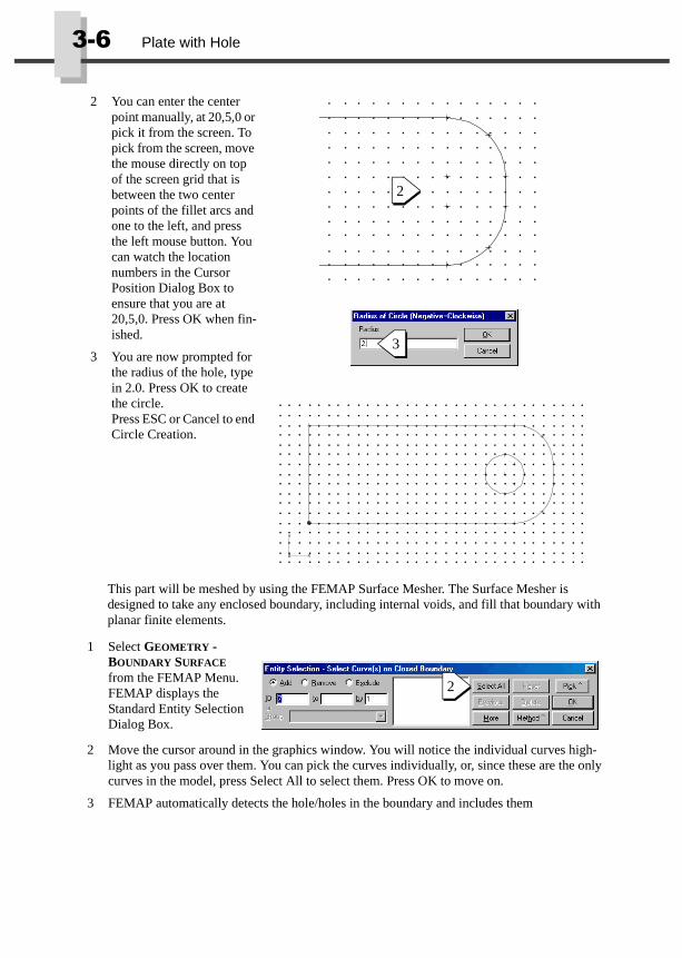
2 You can enter the center point manually, at 20,5,0 or pick it from the screen. To pick from the screen, move the mouse directly on top of the screen grid that is between the two center points of the fillet arcs and one to the left, and press the left mouse button. You can watch the location numbers in the Cursor Position Dialog Box to ensure that you are at 20,5,0. Press OK when fin-ished.
3 You are now prompted for the radius of the hole, type in 2.0. Press OK to create the circle.Press ESC or Cancel to end Circle Creation.
1 Select GEOMETRY - BOUNDARY SURFACE from the FEMAP Menu. FEMAP displays the Standard Entity Selection Dialog Box.
2 Move the cursor around in the graphics window. You will notice the individual curves high-light as you pass over them. You can pick the curves individually, or, since these are the only curves in the model, press Select All to select them. Press OK to move on.
3 FEMAP automatically detects the hole/holes in the boundary and includes them
2
3
X
Y
Z
2

3
/$7(
�:,7+
�+
2/(
Defining Materials and Properties ���
The boundary is displayed as a highlighted entity on top of its underlying geometry.
The geometry creation phase of this example is now complete. From now on we will be creat-ing entities directly related to Finite Element Analysis. First Material and Element Properties will be defined. Then Nodes and Elements will be generated automatically using the underly-ing geometry. Finally Loads and Boundary Conditions will be defined on the finite element mesh.
3.3 Defining Materials and PropertiesBefore any finite elements can be created, we must first define a material.
1 Select MODEL - MATE-RIAL from the FEMAP Menu. FEMAP displays the Define Isotropic Material Dialog Box. You could enter all the physical properties of a material in this box, or to use the library of materials included with FEMAP, Press the Load Button.
2 FEMAP Material Librar-ies are easy to extend with your own materials. The library that ships with FEMAP contains several common material in U.S. (in. lb. sec.) units. In this example select AISI 4130 Steel using the arrow keys or the mouse, and Press OK when finished.
X
Y
Z
1
2
��� Plate with Hole
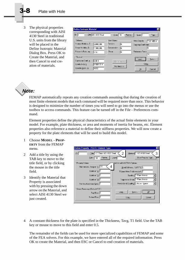
Note:FEMAP automatically repeats any creation commands assuming that during the creation of most finite element models that each command will be required more than once. This behavior is designed to minimize the number of times you will need to go into the menus or use the toolbox to access commands. This feature can be turned off in the File - Preferences com-mand.
Element properties define the physical characteristics of the actual finite elements in your model. For example, plate thickness, or area and moments of inertia for beams, etc. Element properties also reference a material to define their stiffness properties. We will now create a property for the plate elements that will be used to build this model.
3 The physical properties corresponding with AISI 4130 Steel in traditional U.S. units from the library will be placed in the Define Isotropic Material Dialog Box. Press OK to Create the Material, and then Cancel to end cre-ation of materials.
1 Choose MODEL - PROP-ERTY from the FEMAP menu.
2 Add a title by using the TAB key to move to the title field, or by clicking the mouse in the title field.
3 Identify the Material that Property is associated with by pressing the down arrow on the Material, and select AISI 4130 Steel we just created.
4 A constant thickness for the plate is specified in the Thickness, Tavg, T1 field. Use the TAB key or mouse to move to this field and enter 0.5.
The remainder of the fields can be used for more specialized capabilities of FEMAP and some of the FEA solvers. For this example, we have entered all of the required information. Press OK to create the Material, and then ESC or Cancel to end creation of materials.
4
2 3

3
/$7(
�:,7+
�+
2/(
Generation of Nodes and Elements ���
3.4 Generation of Nodes and ElementsWe will now create the actual finite elements by using the FEMAP Surface Mesher.
The part will be meshed totally automatically. The size of the individual elements was deter-mined by the default global mesh size, that you can control. In addition, the number of element generated along each geometric entity can be specified with the Mesh - Mesh Control - Size Along Curve command overriding the global mesh size. In this example, the standard default mesh size of 1.0 was sufficient and did not need to be modified. At this point the display is fairly cluttered with the node and element numbers. We will now use some of the View Options in FEMAP to modify the display and remove unnecessary information.
1 Select MESH - GEOME-TRY-SURFACE from the FEMAP Menu. FEMAP will display the Standard Entity Selection Dialog Box, and prompt you for the Boundary to mesh. Select the Boundary from the screen, or use Select All. Press OK to continue.
2 FEMAP will now display the Generate Boundary Mesh Dialog Box.
A.) Select the Property to be used for the elements gener-ated, and B.) Press OK to generate them. There are many options in the Bound-ary Mesh Dialog Box that provide extensive control over the automatic mesh. For this example we will use the default settings. Defaults have been carefully designed to generate a quality mesh for a wide variety of geometries.
A
B
���� Plate with Hole
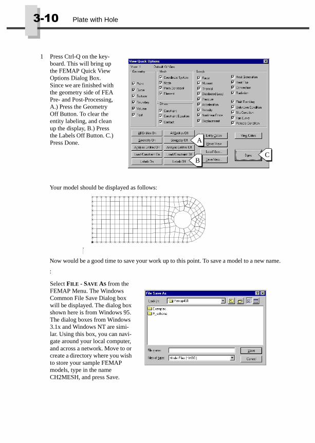
Your model should be displayed as follows:
Now would be a good time to save your work up to this point. To save a model to a new name.
:
1 Press Ctrl-Q on the key-board. This will bring up the FEMAP Quick View Options Dialog Box. Since we are finished with the geometry side of FEA Pre- and Post-Processing, A.) Press the Geometry Off Button. To clear the entity labeling, and clean up the display, B.) Press the Labels Off Button. C.) Press Done.
Select FILE - SAVE AS from the FEMAP Menu. The Windows Common File Save Dialog box will be displayed. The dialog box shown here is from Windows 95. The dialog boxes from Windows 3.1x and Windows NT are simi-lar. Using this box, you can navi-gate around your local computer, and across a network. Move to or create a directory where you wish to store your sample FEMAP models, type in the name CH2MESH, and press Save.
A
BC
Y

3
/$7(
�:,7+
�+
2/(
Loading and Constraining the Model ����
et.
ed e
3.5 Loading and Constraining the ModelRecall that we want to weld and fix the inside of the hole, then pull on the left side of the bracket with a total force of 5,500 pounds.
We will now add the loads and constraints required to perform a static finite element analysis, first we must first create an empty Load Set. FEMAP supports multiple load and constraint sets to allow you to define more than one loading condition or constraint condition for the same finite element model.
Similar to Load Sets, there are also Constraint Sets for storing different boundary conditions for your model. To create the first empty Constraint Set, select MODEL - CONSTRAINT - SET from the menu, type a descriptive name, such as “Welded Hole” and create the empty s
Let’s first constrain the part. Constraints define how a part is held in reaction to the appliloads. In this case we will completely fix all the nodes around the hole as if the plate werwelded to a significantly stiff underlying structure.
To create the empty load set, choose MODEL - LOAD - SET from the menu and add a descrip-tive name in the Title box. Press OK to create the Set.
1 Choose MODEL - CON-STRAINT - NODAL from the menu. Again FEMAP will display the Standard Entity Selection Dialog Box. Instead of box picking this time, we will circle pick the nodes around the hole.
2 Zoom in on the area around the circle. To do so, press the Zoom Icon on the toolbar.
2

���� Plate with Hole
3 Now pick a box around the hole with picks at A and B.
4 Circle picking is similar to box picking, but instead of pressing and holding the shift key, you press and hold the control key. The trick in circle picking is to make the first pick A.) at the center of the cir-cle and then move out to the outside radius B.)
5 FEMAP will now fill in the nodes selected within the circle. Press OK to select these nodes.
6 You will now see the Create Nodal Constraints/DOF Dialog Box. Press the Fixed Button to constrain all six degrees of freedom at this location. Press OK to create the constraints. Press the ESC Key or Press Cancel to end creation of constraints.
A
B
X
Y
Z
V1L1C1
A
B
6

3
/$7(
�:,7+
�+
2/(
Loading and Constraining the Model ����
The model should look like the one below. If you do not see all of your model, press Ctrl-A to Autoscale the view.
We will now apply a load to the model along the left hand side, in the negative x direction totaling 5,500 pounds.
1 Select MODEL - LOAD - NODAL from the FEMAP menu. FEMAP will now display the Standard Entity Selection Box requesting nodes.
2 You could pick the 11 nodes at the end of this part one by one, or instead, use the box-picking capability of FEMAP. To box pick, press and hold down the shift key, then, A.) move the mouse to one corner of the rect-angle you wish to select inside of, and press the left mouse button and drag the mouse to B.) the other corner of the region. You will see a dashed rectangle on screen indicating the region that will be selected.
3 FEMAP will fill in the Entity Selection Dialog box with the nodes inside the rectangle. Press OK to select these nodes.
X
Y
Z
V1C1
X
Y
Z
V1C1
A
B

���� Plate with Hole
Running the AnalysisThe model building stage is now complete. The model is ready for analysis by any one of a number of finite element codes that FEMAP supports. Refer to the translation section of the FEMAP User Guide and your analysis program documentation to analyze this model. Typi-cally, select FILE - EXPORT - ANALYSIS MODEL from the FEMAP menu. Choose the analysis program that you have access to, set the Analysis Type to Static, and press OK. FEMAP will then lead you through the creation of an input deck with dialog boxes custom designed to properly set up the analysis for your particular solver.
Once you have created an input file for your FEA program, you need to run that program.
3.6 Review the ResultsAfter solution, FEMAP can read the output results for post-processing. Reading output results is similar to writing the model for analysis, select FILE - IMPORT - ANALYSIS RESULTS from the FEMAP menu, set the translator to your FEA program, and then press OK. FEMAP will lead you through the rest of the process based on requirement of your particular analysis code. Once read in, the results are available for a wide array of graphical and numerical post-pro-cessing.
If you do not have access to a finite element analysis program, the results of analyzing this sample model are available on the diskette included with this manual. Select File - Open from the FEMAP menu, navigate to the directory where you installed the example problems for this manual. In the /examples subdirectory, open CH3POST.MOD.
4 FEMAP now displays the Create Nodal Loads Dia-log Box. Move to the TX (Translation Degree of Freedom, X-Direction) and enter a value of nega-tive 500 (-500.0). Press OK to create the loads. Press ESC or Cancel to end creating nodal loads. You will now see the loads on your model:
4

3
/$7(
�:,7+
�+
2/(
Review the Results ����
Viewing the Deformed Model:
Viewing the Stress DistributionSimilar to turning on the deformed plot, you can return to View - Select and change the Con-tour Style option from None - Model Only to Contour and pressing OK. FEMAP displays the
1 Choose VIEW - SELECT from the menu. The View - Select command determines how your model will appear on screen. To view the model deformed by the results of your analysis, A.) change the Deformed Style to Deform. To specify exactly what data to use for Post-Processing, B.) Press the Deformed and Contour Data Button.
2 The Select Post-Processing Dia-log Box is now displayed. Here, you specify what data is used for on-screen Post-Processing. Data from multiple analysis runs or multiple Load Set/Con-straint Set combinations will be stored in multiple Output Sets. The combo box at A.) is used to specify which Output Set the results will be obtained from, and the B.) Deformation and C.) Contour combo boxes are used to choose which particular pieces of output data are used for the Deformed Style and Contour Style options in the previous View - Select Dialog Box. Press OK to accept these choices, and then Press OK in the View Select Dialog box to activate the Deformed view.
A
B
A
B
C
X
Y
Z
V1L1C1
Output S et: MS C/NAS T RAN Case 1Deformed(0.00085): T otal T rans lation

���� Plate with Hole
model with a color representation of the stress levels superimposed on top of the deformed shape.
This chapter was designed to provide you with an overview of working with FEMAP, and to let you work through one sample problem from start to finish. The following chapters contain different types of examples to give you a broad range or experience with FEMAP.
X
Y
Z
1681.
1587.
1494.
1400.
1307.
1214.
1120.
1027.
933.3
839.8
746.4
653.
559.5
466.1
372.6
279.2
185.8
V1L1C1
Output S et: MS C/NAS T R AN Case 1Deformed(0.00085): T otal T rans lationContour: Plate T op VonMises S tres s

Turbine Blade 9
This example will illustrate some simple solid modeling in FEMAP. First we will read in an IGES trimmed surface part. Then in FEMAP we will stitch the sur-faces into a solid, and then modify the solid so we can get a proper FEA mesh. We can then add loads and constraints directly to the geometry of the solid model. The final step in analysis prepara-tion will be to create a material and then use the automatic tetrahedral element mesher to mesh the solid. To complete this example you must have purchased FEMAP Professional.
Note:You will not be able to save your model file or export to an analysis program if you are using the 300-Node Demonstration version. A file with results is provided to use for the postpro-cessing section of this example.
First start FEMAP and create a new model, or if FEMAP is already running, select FILE - NEW from the menu.
9.1 Creating the GeometryReading the IGES File
1 Select FILE-IMPORT-GEOMETRY from the FEMAP menu. The Windows File Open Common Dialog Box appears. Navigate to the \Examples directory and A) Select the TurbineBlade.igs file and B) Press open.
A
B

��� Turbine Blade
The messages and lists window will tell you what has been read and also log any errors in the import operation.
Stitch the IGES trimmed surfaces into a solid
The messages and lists window informs you that the model has been stitched and conforms to Parasolid modeling tolerances. This simply means that the stitching operation was successful and the model is now a FEMAP solid that can be operated on with FEMAP geometry com-mands.
Rotate the View
2 The IGES Read Options dialog box appears. The default values should work for most IGES files and they will here, so press OK.
1 Choose GEOMETRY-SOLID-STITCH. The Standard entity selection dialog box appears and prompts you to select the surfaces to stitch. For this model A) select all surfaces and B) press OK.
1 Choose VIEW - ROTATE from the FEMAP Menu (or use the Ctrl-R or F8 short-cut keys) and you will see the View Rotate Dialog Box. There are several pre-defined 3-D views that you can select from, you may want to experiment and press some of them. Before leaving View Rotate, press Dimetric and then OK to dismiss the View Rotate Dialog Box.
2
1
1

7
85%,1(
�%
/$'(
Creating the Geometry ���
so that m a
Split Surface Along Constant UV LineWe now want to split the two large surfaces that make up the blade at the blade’s edges the mesh will not wrap across the edges. We will do this by imprinting a curve made froconstant parametric value of the surface.
1 Choose GEOMETRY-CURVE FROM SURFACE-UPDATE SUR-FACES. This toggles whether or not the created curve imprints on and splits the surface or surfaces it intersects. We want this option on.
2 Choose GEOMETRY-CURVE FROM SURFACE-PARA-METRIC CURVE. FEMAP prompts you to select a sur-face. Move the cursor to highlight surface A and press the left mouse button to pick it. Press OK.
3 FEMAP prompts you for a location for the curve. Press the methods button and choose Midpoint from the list. Move the cursor over curve B in the diagram above to high-light it and select it with the left mouse button. Press OK.
4 FEMAP prompts you for a parametric curve direction. You can use the surface lines to determine the proper direction. By default FEMAP draws 3 divisions in the U direction and 4 in the V direc-tion. So in this case select the U direction and press OK.
X
Y
Z
A
B
CD
1

��� Turbine Blade
9.2 Loads and ConstraintsAdd Loads on Geometry
5 Repeat the above procedure this time using surface C and curve D. There should now be curves along the edges as shown here.
1 Choose MODEL-LOAD-ON SURFACE, FEMAP prompts you to select a load set or create a new one. Type in a title and press OK.
2 FEMAP now asks you to select the surfaces to apply the load. Pick the two large surfaces on the top of the blade and press OK.
X
Y
Z

7
85%,1(
�%
/$'(
Loads and Constraints ���
Add Constraints on Geometry
3 FEMAP displays the Load on Surfaces dialog box. A) Select pressure as the load type B) Leave the direction as normal to ele-ment face C) Enter a value of 10 and D) Press OK.
4 Repeat the procedure above, this time selecting the bottom surfaces of the blade and entering a pressure of negative ten (-10).
1 Choose MODEL-CON-STRAINT-ON SURFACE. FEMAP prompts you to select a constraint set or create a new one. Type in a name and press OK.
2 FEMAP prompts you to select surfaces. Pick the two halves of the cylinder at the bottom of the blade and press OK.
B
D
CA

��� Turbine Blade
9.3 Meshing the SolidSuppress Small Features
The small hole in the base of the turbine blade will not affect the results of the analysis but will cause the mesh to condense in that area. To reduce the number of elements and our overall problem size we will suppress this small hole before meshing.
3 Constraints on surfaces are always relative to the global coordinate system and can only be fixed, pinned or have no rota-tions. Make these sur-faces fixed. Press OK to create the constraints, press cancel to end the command.
1 Choose MESH-MESH CONTROL-FEATURE SUPPRESSION. Select the turbine blade as the solid model.

7
85%,1(
�%
/$'(
Meshing the Solid ���
Meshing the Model
2 In the feature suppression dialog box, A) Select manual, B) Select remove and C) Press the Loops button.
3 Select one of the two curves that make up the top of the small hole and press OK. The surfaces of the hole should be grayed out indicating that they are suppressed.
1 Choose MESH-GEOME-TRY-SOLIDS.
2 Change the Element Size to 0.05 and press OK. This element size is determined by the shape and size of the various fea-tures of the model. The default values determined by FEMAP are usually adequate to produce a good mesh. How-ever, as you gain experience with the solid mesher you may find that a slightly larger element size will still give you a good mesh but greatly reduce the number of elements. On the other hand some parts may need a smaller element size to produce a good mesh in certain areas. Also, keep in mind that you can specify mesh spacing and mesh hard points on all curves and surfaces individually. This is often the best way to get the best mesh although it does take more time and careful planning.
A
B C

��� Turbine Blade
When the model finishes meshing it will be ready for analysis.
Note:You should always check the shapes of your elements before you run an analysis. Badly dis-torted elements can cause incorrect results and analysis failure. For information on checking element distortion refer to the FEMAP Command Reference.
3 Since no material has been created FEMAP prompts you to make one. You can enter in values or press the Load button to bring up the material library.
4 The material library shipped with FEMAP contains material proper-ties using English units (lb, in, sec). You can cre-ate your own materials and store them in this library or create your own library. For this example select a material from this library and press OK.
Note:Remember, there are no units in FEMAP. All dimensions must be kept consistent with the unit system you use to define your material properties.
5 Press OK in the define material dialog box when the properties have been loaded.
6 The automesh solids dia-log box appears. Leave the values as the defaults and press OK.
3
4

7
85%,1(
�%
/$'(
PostProcessing ���
9.4 PostProcessingReading in Results
For this example we have included a FEMAP model file with results included that you can use for Postprocessing. If you have run your own analysis you may use those results.
Graphical PostprocessingThis section will take you through some of the ways you can use FEMAP to view analysis results.
1 Select FILE - OPEN. The standard file open dialog box appears. Navigate to the /Examples directory and choose the CH9Post.Mod file. Press open.
1 A) Press the view style button on the toolbar and choose solid. B) Press the view style button on the toolbar and choose Ren-der. This puts you in Ren-der mode which allows dynamic pan, zoom and rotate of solid contoured models as well as dynamic isosurfaces and sections cuts and also speeds up general graph-ics.
A
B

���� Turbine Blade
2 Press Ctrl-Q or the view quick options toolbar but-ton to bring up the view quick options menu. Press the geometry off button and the labels off button.
3 Select VIEW-SELECT, press F5 or the view select button on the toolbar to bring up the view select dialog box. Set the Deform Style to Deform and the Contour Style to Contour. Press the Deformed and Contour Data Button.
4 This brings up the Select PostProcessing Data dia-log box. A) Select an out-put set. B) Select an output vector to use for the model deformation. C) Select an output vector to use for the contour plot. Press OK. Press OK in the view select dialog box.
5 In Render mode simply click the left mouse but-ton in the graphics win-dow and drag the cursor. The model will rotate in XY. You can also use the same Dynamic Display options with the Alt, Ctrl, and Shift (Rotate Z, Pan, Zoom)
B
A
C

7
85%,1(
�%
/$'(
PostProcessing ����
6 Select VIEW-SPECIAL POST-DYNAMIC CUTTING PLANE. Move the slider bar to move the cutting plane through the model. Press the plane button to define a different cutting plane using the standard plane definition dialog box. Press the Dynamic Display button to rotate the view of the cutting plane. Press OK when done.
7 Select VIEW-SPECIAL POST-DYNAMIC ISOSURFACE. Move the slider bar to change the value of the isosurface being shown. The isosurface itself is calculated from the output vector chosen for the contour vector. Put the cursor in the value box, enter a value and press apply to see an isosurface at that value. Rotate the view if you would like. Press OK when done.
8 Select VIEW-SELECT, press F5 or the view select button on the toolbar to bring up the view select dialog box. Set the Con-tour Style to IsoSurface. Press OK.
9 Select VIEW-OPTIONS or press F6. A) Pick post-processing as the category B) Pick IsoSurface as the option. C) Check the Contour Deformed box to see the deformed output vector contoured on the isosurface. Press Apply. Change the IsoSurface At value and press Apply to see a different isosurface. Press OK. Use VIEW-SPECIAL POST-DYNAMIC ISOSURFACE to dynamically change the isosur-face value.
10 Select VIEW-SELECT, press F5 or the view select button on the toolbar to bring up the view select dialog box. Set the Deform Style to Animate and the Contour Style to Contour. Press OK.
C
A
B

���� Turbine Blade
Experiment with some of the other postprocessing and viewing options on your own.
11 Select VIEW-OPTIONS or press F6. In the Postpro-cessing category select Animated Style. Change the number of frames to get a smoother animation. Increase the delay to slow down the animation. Select the Contour/Crite-ria Levels option. Check the animate box to ani-mate the contour colors as well as the deformation.

Hex Meshing Overview 15
This example requires FEMAP Parasolid modeler to complete. If you have the 300-Node ver-sion you will not be able to save or export the model.
15.1 IntroductionThis is an example of how solids can be subdivided to facilitate hex meshing in FEMAP. It assumes you are familiar with FEMAP and do not need step by step instructions for all com-mands. It is intended to give you one method of approaching the problem of hex meshing solid models, and demonstrates only a few of the commands that can be used to hex mesh in FEMAP. For more descriptions and methods refer to the Commands manual and the User Guide.
15.2 Importing the Geometry
1 Select FILE - IMPORT - GEOMETRY from the FEMAP menu.
2 FEMAP displays the standard Win-dows File Open Dialog Box. Maneuver to the /examples subdi-rectory and A.) select the Ch15hexmesh.x_t file, and B.) Press Open.
3 The FEMAP Solid Model Read Options Dialog Box is displayed, providing several options for how to treat the incoming data. Set the Geometry Scale Factor to 39.37 and press OK.
A
B

���� Hex Meshing Overview
15.3 Subdividing the Solid
4 A) Press the view style button on the toolbar and choose Rendered Solid.
5 Left click and drag in the graphics window to dynamically rotate the model.
1 We first want to slice the solid with three planes. Use the Geom-etry Solid Slice com-mand three times. Be sure to select all the solids each time. Using whatever method you please, slice the solid along the planes of the curves pointed to by 1,2 and 3
A
3
2
1
1
2
3

+
(;
�2
9(59,(:
Subdividing the Solid ����
2 You should end up with seven separate solids. The picture is an exploded view to clearly show the sepa-rate solids. Your view will still look like the previous one.
3 The square in the cen-ter is not a hex-mesh-able solid. We have learned from experi-ence that a good way to subdivide this part is to cut it into sixths (A), and then add pieces back together to form three six sided vol-umes(B) that are easily hex meshed.
4 Keep in mind that you need to have surface meshes that match. The easiest way to ensure this on this model is to also slice the radiused solids. Try to produce the 12 distinct solids at right. The picture is an exploded view to clearly show the sepa-rate solids.
A
B

���� Hex Meshing Overview
15.4 Preparing for Meshing
1 Select Mesh - Mesh Control - Size on Solid and select all the solids. In the Auto-matic Mesh Sizing dia-log box choose Hex Meshing and set the Min Elements on Edge to 4. The rest of the defaults are fine so press OK.
2 The sizes are set and colors are updated to show which solids are hex-meshable and which surfaces have been linked.
1
2

+
(;
�2
9(59,(:
Meshing ����
15.5 Meshing
1 Select Mesh Geometry Hex Mesh Solids and select all the solids.
2 Since no material has been created FEMAP prompts you to make one. You can enter in values or press the Load button to bring up the material library.
3 The material library shipped with FEMAP contains material proper-ties using English units (lb, ft, sec). You can cre-ate your own materials and store them in this library or create your own library. For this example select a material from this library and press OK.
Note:Remember, there are no units in FEMAP. All dimensions must be kept consistent with the unit system you use to define your material properties. Always make sure this is cor-rect from the beginning because it is extremely difficult to correct inconsistencies in units once the model is built.
4 Press OK in the define material dialog box when the properties have been loaded.
5 The Hex Mesh Solids dia-log box appears. Leave the values as the defaults and press OK.
3
4
���� Hex Meshing Overview
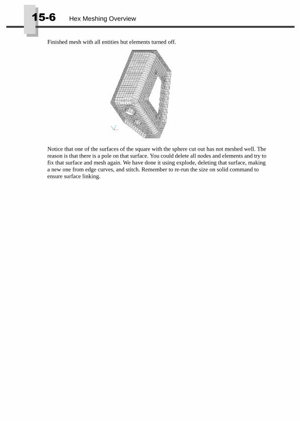
Finished mesh with all entities but elements turned off.
Notice that one of the surfaces of the square with the sphere cut out has not meshed well. The reason is that there is a pole on that surface. You could delete all nodes and elements and try to fix that surface and mesh again. We have done it using explode, deleting that surface, making a new one from edge curves, and stitch. Remember to re-run the size on solid command to ensure surface linking.

Hex Meshing 16
This example requires FEMAP Parasolid modeler to complete. If you have the 300-Node ver-sion you will not be able to save or export the model.
16.1 Importing the Geometry
1 Select FILE - IMPORT - GEOMETRY from the FEMAP menu.
2 FEMAP displays the stan-dard Windows File Open Dialog Box. Maneuver to the /examples subdirec-tory and
A.) Select the Ch16hexmesh.x_t file,
B.) Press Open.
3 The FEMAP Solid Model Read Options Dialog Box is displayed, providing several options for how to treat the incoming data. Set the Geometry Scale Factor to 39.37 and press OK.
A) Press the view style button on the toolbar and choose solid.
B) Press the view style button on the toolbar and choose Render.
A
B
A
B

���� Hex Meshing
16.2 Subdividing the Solid
Left click and drag in the graphics window to dynamically rotate the model.
1 We want to subdivide this solid into the ten indepen-dent solids shown here. The solids are shown exploded for viewing only.
2 Start with Geometry - Solid - Embed Face, pick surface A. Repeat this command for surfaces B and C.
CB
A

+
(;
�0
(+6,1*
Meshing ����
16.3 MeshingWe will begin setting up a hex mesh using the default approaches and let FEMAP set up the mesh automatically. You will find that the defaults provide a good hex mesh but we will mesh the solid again using some of the more advanced options to obtain a mapped mesh.
3 Now use Geometry-Solid-Extrude and press the surface button (A) and pick surface A above. Change the direction to negative (B) and enter a depth of 10 (C).
4 Next pick Geometry-Solid-Embed. Pick the solid with the tube as the base solid at (A), and the one you just created at (B) as the one to embed.
5 You now need to make two slices. Slice the tube off at the top of the radius (C), and slice the three solids (1,2,3) near the tube in half. Refer to the exploded diagram if you have difficulty visualiz-ing the individual solids.
CBA
B
A
C
2
1
3

���� Hex Meshing
16.3.1 Free Meshing1 Use Mesh-Mesh Con-
trol-Size On Solid, select all solids and
(A) Turn on Size for Hex Meshing, and
(B) Enter a Min Elements on Edge of 2.
This command will also link all the shared sur-faces to ensure a consis-tent mesh.
2 Use the Mesh-Geometry-Hexmesh Solids com-mand and select all the solids to hex mesh. If you have properly set mesh sizes and linked surfaces, the hex mesh should run automatically.
A
B
+
(;
�0
(+6,1*
Mapped Meshing ����
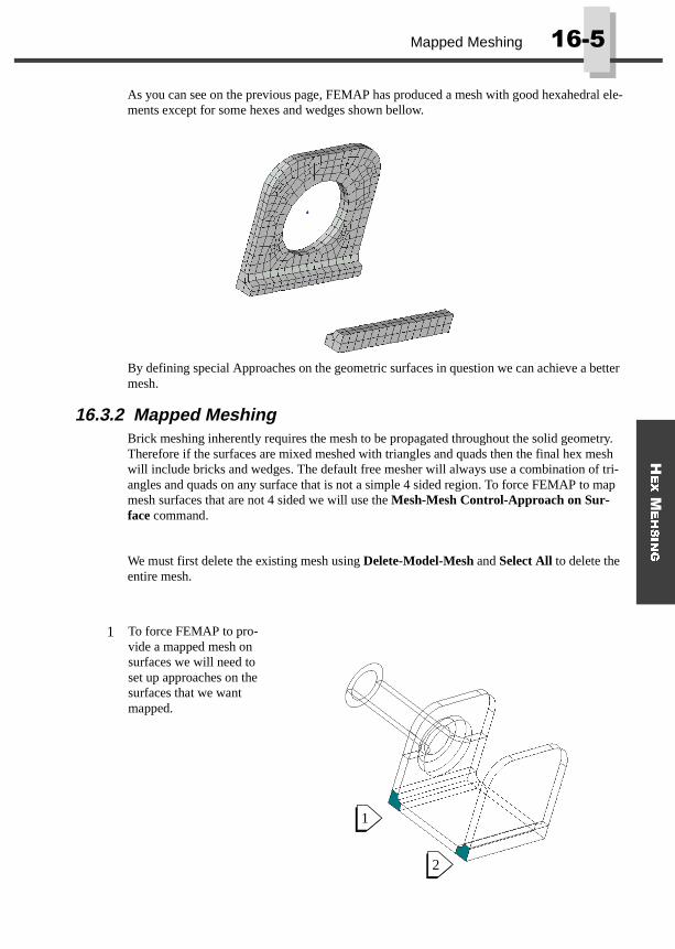
As you can see on the previous page, FEMAP has produced a mesh with good hexahedral ele-ments except for some hexes and wedges shown bellow.
By defining special Approaches on the geometric surfaces in question we can achieve a better mesh.
16.3.2 Mapped MeshingBrick meshing inherently requires the mesh to be propagated throughout the solid geometry. Therefore if the surfaces are mixed meshed with triangles and quads then the final hex mesh will include bricks and wedges. The default free mesher will always use a combination of tri-angles and quads on any surface that is not a simple 4 sided region. To force FEMAP to map mesh surfaces that are not 4 sided we will use the Mesh-Mesh Control-Approach on Sur-face command.
We must first delete the existing mesh using Delete-Model-Mesh and Select All to delete the entire mesh.
1 To force FEMAP to pro-vide a mapped mesh on surfaces we will need to set up approaches on the surfaces that we want mapped.
2
1

���� Hex Meshing
2 Use Mesh-Mesh Con-trol-Approach on Sur-face
FEMAP will ask you to pick the surface you wish to put a approach on.Choose surface 1 on the previous page.
When the Surface Approach dialog box comes up select A.) Mapped - Four Corner
3 Since this surfaces has more than 4 corners you must specify which cor-ners you want FEMAP to map between.
B.) Choose the corners as shown for the first surface and say OK. The com-mand will auto repeat allowing you to choose surface 2 on the previous page and select the four corners from the diagram to the right.
Now we will set up sur-faces 3 and 4 for mapped meshing. Use Mesh-Mesh Control-Approach on Surface again.
FEMAP will ask you to chose the surface to set the approach on Select surface 3 and 4 from the diagram to the right.
A
B
1
2
3
4
3
4
21
3
4

+
(;
�0
(+6,1*
Mapped Meshing ����
By applying approaches on surfaces of the model the quality of the mesh can be greatly improved.
After selecting the sur-faces choose the Mapped Four Corner approach and select the four points as shown to the right.Then say OK.
4
5
Mesh all of the solids using Mesh-Mesh Con-trol-Size On Solid, select all solids and
(A) Turn on Size for Hex Meshing, and
(B) Enter a Min Elements on Edge of 3. Select Mesh-Geomerty-Hexmesh Solids and select all of the solids to hex mesh.
1
32
4
A
B