Plate Element2

8/8/2019 Plate Element2

http://slidepdf.com/reader/full/plate-element2 1/16

.

2 6Thin Plate Elements:Overview

26–1



Chapter 26: THIN PLATE ELEMENTS: OVERVIEW 26 – 2

TABLE OF CONTENTS

Page

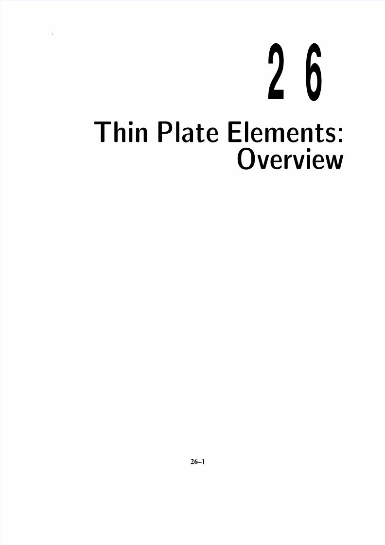
§26.1. An Overview of KTP FE Models 26–4§26.1.1. Triangles . . . . . . . . . . . . . . . . . . . 26–4§26.1.2. A Potpourri of Freedom Congurations . . . . . . . . 26–5§26.1.3. Connectors . . . . . . . . . . . . . . . . . . 26–6

§26.2. Convergence Conditions 26–7§26.2.1. Completeness . . . . . . . . . . . . . . . . . 26–7§26.2.2. Continuity Games . . . . . . . . . . . . . . . . 26–7

§26.3. *Kinematic Limitation Principles 26–9§26.3.1. Limitation Theorem I . . . . . . . . . . . . . . 26–10§26.3.2. Limitation Theorem II . . . . . . . . . . . . . . 26–10§26.3.3. Limitation Theorem III . . . . . . . . . . . . . . 26–11

§26.4. Early Work 26–12§26.4.1. Rectangular Elements . . . . . . . . . . . . . . 26–12§26.4.2. Triangular Elements . . . . . . . . . . . . . . 26–13§26.4.3. Quadrilateral Elements . . . . . . . . . . . . . . 26–14

§26.5. More Recent Work 26–14

26– 2



26– 3

TABLE OF CONTENTS

Page

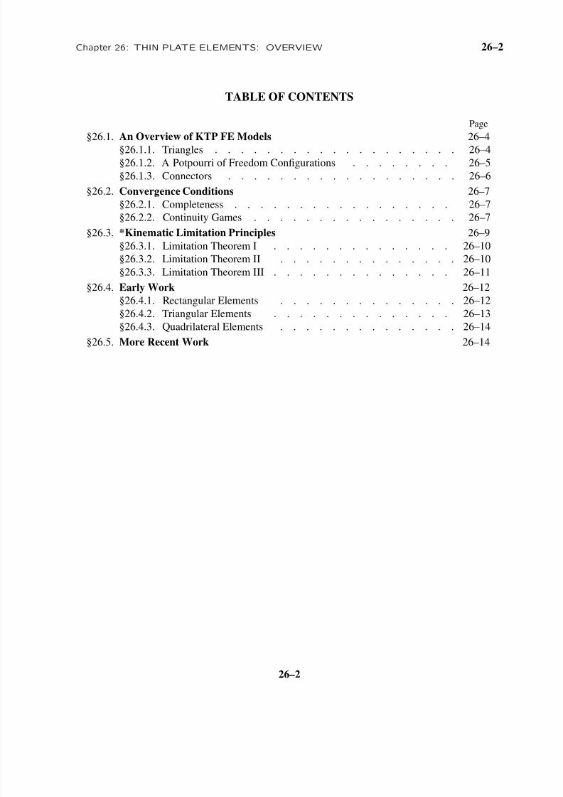
§26.1. An Overview of KTP FE Models 26–4§26.1.1. Triangles . . . . . . . . . . . . . . . . . . 26 –4§26.1.2. A Potpourri of Freedom Con gurations . . . . . . . . . 26 –5§26.1.3. Connectors . . . . . . . . . . . . . . . . . 26 –6

§26.2. Convergence Conditions 26–7§26.2.1. Completeness . . . . . . . . . . . . . . . . . 26 –7§26.2.2. Continuity Games . . . . . . . . . . . . . . . 26 –7

§26.3. *Kinematic Limitation Principles 26–9§26.3.1. Limitation Theorem I . . . . . . . . . . . . . . . 26 –10§26.3.2. Limitation Theorem II . . . . . . . . . . . . . . 26 –10§26.3.3. Limitation Theorem III . . . . . . . . . . . . . . 26 –11

§26.4. Early Work 26–12§26.4.1. Rectangular Elements . . . . . . . . . . . . . . 26 –12§26.4.2. Triangular Elements . . . . . . . . . . . . . . . 26 –13§26.4.3. Quadrilateral Elements . . . . . . . . . . . . . . 26 –14

§26.5. More Recent Work 26–14

26– 3




This Chapter presents an overview of nite element models for thin plates usinf the Kirchhoff Platebending (KPB) model. The derivation of shape functions for the triangle geometry is covered inthe next chapter.

§26.1. An Overview of KTP FE Models

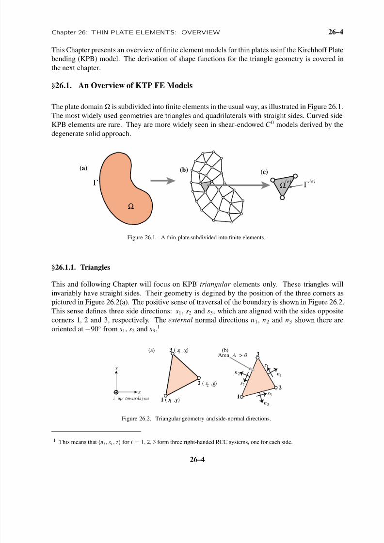
The plate domain is subdivided into nite elements in the usual way, as illustrated in Figure 26.1.The most widely used geometries are triangles and quadrilaterals with straight sides. Curved sideKPB elements are rare. They are more widely seen in shear-endowed C 0 models derived by thedegenerate solid approach.

Ω

ΩΓ Γ

(a) (b) (c)(e)(e)

Figure 26.1. A thin plate subdivided into nite elements.

§26.1.1. Triangles

This and following Chapter will focus on KPB triangular elements only. These triangles willinvariably have straight sides. Their geometry is degined by the position of the three corners aspictured in Figure 26.2(a). The positive sense of traversal of the boundary is shown in Figure 26.2.This sense de nes three side directions: s1 , s2 and s3 , which are aligned with the sides oppositecorners 1, 2 and 3, respectively. The external normal directions n 1 , n 2 and n 3 shown there areoriented at − 90 from s1 , s2 and s3 .1

1 ( x ,y)11

2 ( x ,y)22

3 ( x ,y)33(a) (b)

x

y

z up, towards you

Area A > 0 3

2

1s3

n3

s1

n1

s2

n 2

Figure 26.2. Triangular geometry and side-normal directions.

1 This means that n i , si , z for i = 1, 2, 3 form three right-handed RCC systems, one for each side.

26– 4



26– 5 §26.1 AN OVERVIEW OF KTP FE MODELS

11

2 2

3

4 5

6

7

08

9

(b)(a) (c)

(f)

w

w

ww

w

w

w

w

w

w

1

w1

w1

s31ws32w

s11w

s13w

s23w

s21w

12

3

0

n21θ n32θ

n11θ

n13θn23θ

n31θ

2 w2w2

3 w3

w3

45

6

7 8

9 0

3

0

s3

s1

s2

w11

2

3

0 x3θ

y3θ x3θ

y3θ

y1θ

x1θw2

w3

12

(d)

w1

n31wn32w

n12w

n13wn23w

n21ww2

w33

0

(e)

w1 12

3

0

s21θ s32θ s11θ

s13θ

s23θ

s31θw2

w3

s3

s1

s2

n3

n3

n1

n1

n2

n2

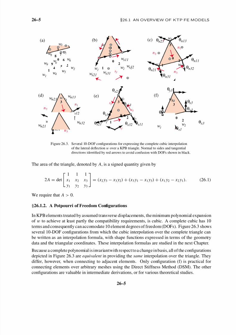
Figure 26.3. Several 10-DOF con gurations for expressing the complete cubic interpolationof the lateral de ection w over a KPB triangle. Normal to sides and tangentialdirections identi ed by red arrows to avoid confusion with DOFs shown in black.

The area of the triangle, denoted by A, is a signed quantity given by

2 A = det 1 1 1 x1 x2 x3

y1 y2 y3

= ( x2 y3 − x3 y2) + ( x3 y1 − x1 y3) + ( x1 y2 − x2 y1 ). ( 26 .1)

We require that A > 0.

§26.1.2. A Potpourri of Freedom Con gurations

In KPB elements treated by assumed transverse displacements, the minimum polynomial expansionof w to achieve at least partly the compatibility requirements, is cubic. A complete cubic has 10terms and consequently can accomodate 10 element degrees of freedom(DOFs). Figure 26.3 showsseveral 10-DOF con gurations from which the cubic interpolation over the complete triangle canbe written as an interpolation formula, with shape functions expressed in terms of the geometrydata and the triangular coordinates. These interpolation formulas are studied in the next Chapter.

Because a complete polynomial is invariantwith respect toa change inbasis, all of the con gurationsdepicted in Figure 26.3 are equivalent in providing the same interpolation over the triangle. Theydiffer, however, when connecting to adjacent elements. Only con guration (f) is practical forconnecting elements over arbitrary meshes using the Direct Stiffness Method (DSM). The othercon gurations are valuable in intermediate derivations, or for various theoretical studies.

26– 5




12

(a) (b)

s31w

(e1) (e1)

(e2) (e2)

1 12 2

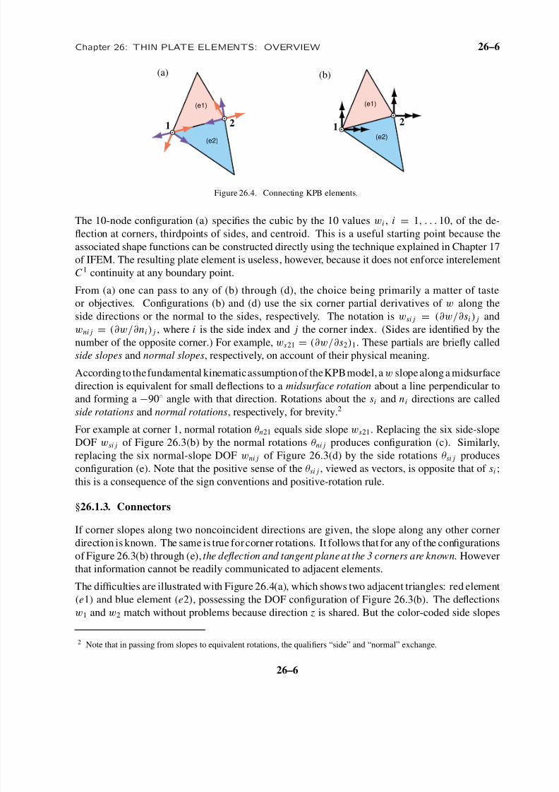
Figure 26.4. Connecting KPB elements.

The 10-node con guration (a) speci es the cubic by the 10 values w i , i = 1, . . . 10, of the de-ection at corners, thirdpoints of sides, and centroid. This is a useful starting point because theassociated shape functions can be constructed directly using the technique explained in Chapter 17of IFEM. The resulting plate element is useless, however, because it does not enforce interelement

C 1

continuity at any boundary point.From (a) one can pass to any of (b) through (d), the choice being primarily a matter of tasteor objectives. Con gurations (b) and (d) use the six corner partial derivatives of w along theside directions or the normal to the sides, respectively. The notation is w si j = (∂w/∂ si ) j andw ni j = (∂w/∂ n i ) j , where i is the side index and j the corner index. (Sides are identi ed by thenumber of the opposite corner.) For example, w s21 = (∂w/∂ s2 )1 . These partials are brie y calledside slopes and normal slopes , respectively, on account of their physical meaning.

According to thefundamental kinematicassumptionof theKPBmodel, a w slope along a midsurfacedirection is equivalent for small de ections to a midsurface rotation about a line perpendicular toand forming a − 90 angle with that direction. Rotations about the si and n i directions are called

side rotations and normal rotations , respectively, for brevity.2

For example at corner 1, normal rotation θn21 equals side slope w s21 . Replacing the six side-slopeDOF w si j of Figure 26.3(b) by the normal rotations θni j produces con guration (c). Similarly,replacing the six normal-slope DOF wni j of Figure 26.3(d) by the side rotations θsi j producescon guration (e). Note that the positive sense of the θsi j , viewed as vectors, is opposite that of si ;this is a consequence of the sign conventions and positive-rotation rule.

§26.1.3. Connectors

If corner slopes along two noncoincident directions are given, the slope along any other cornerdirection is known. The same is true for corner rotations. It follows that for any of the con gurations

of Figure 26.3(b) through (e), the deection and tangent plane at the 3 corners are known . Howeverthat information cannot be readily communicated to adjacent elements.

The dif culties are illustrated with Figure 26.4(a), which shows two adjacent triangles: red element(e1) and blue element (e2) , possessing the DOF con guration of Figure 26.3(b). The de ectionsw 1 and w 2 match without problems because direction z is shared. But the color-coded side slopes

2 Note that in passing from slopes to equivalent rotations, the quali ers “side ” and “normal ” exchange.

26– 6



26– 7 §26.2 CONVERGENCE CONDITIONS

do not match. 3 For more elements meeting at a corner the result is chaotic.

To make the element suitable for implementation in a DSM-based program, it is necessary totransform slope or rotational DOFs to global directions . The obvious choices are the midsurfaceaxes x , y. Most FEM codes use rotations instead of slopes since that simpli es connection of different element types (e.g., shells to beams) in three dimensions. Choosing corner rotations θ xi

and θ yi as DOF we are led to the con guration of Figure 26.3(f). As illustrated in Figure 26.4(b),the connection problem is solved and the elements are now suitable for the DSM.

§26.2. Convergence Conditions

The foregoing exposition has centered on displacement assumed elements where w is the mastereld. Element stiffness equations are obtained through the Total Potential Energy (TPE) variationalprinciple presented in the previous Chapter. The completeness and continuity requirements aresummarized in §23.3 on the basis of a variational index mw = 2. These are now studied in moredetail for cubic triangles.

§26.2.1. Completeness

The TPE variational index mw = 2 requires that all w -polynomials of order 0, 1 and 2 in x , ybe exactly represented over each element. Constant and linear polynomials represent rigid bodymotions, whereas quadratic polynomials represent constant curvature states.

Now if w is interpolated by a complete cubic, the ten terms 1, x , y, x 2 , x y , y2 , x 3 , x 2 y, x y2 , y3are automatically present for any freedom con guration. This appears to be more than enough.Nothing to worry about, right? Wrong. Preservation of such terms over each triangle is guaranteedonly if full C 1 continuity is veri ed. But, as discussed below, attaining C 1 continuity continuity isdif cult. To get it one while sticking to cubics one must makesubstantial changes in the constructionof w . Since those changes do not necessarily preserve completeness, that requirement appears as ana posteriori constraint. Alternatively, to make life easier C 1 continuity may be abandoned exceptat corners. If so completeness may again be lost, for example by a seemingly harmless staticcondensation of w 0 . Again this has to be kept as a constraint.

The conclusion is that completeness cannot be taken for granted in displacement-assumed KPBelements. Gone is the “IFEM easy ride ” of isoparametric elements for variational index 1.

§26.2.2. Continuity Games

To explain what C 1 interelement continuity entails, it is convenient to break this condition into twolevels: 4

C 0 Continuity . The element is C 0 compatible if w over any side is completely speci ed by DOFson that side.

C 1 Continuity . The element is C 1 compatible if it is C 0 compatible, and the normal slope ∂w/∂ nover any side is completely speci ed by DOFs on that side.

3 Positive slopes along the common side point in opposite directions.

4 It is tacitly assumed that the condition is satis ed inside the element.

26– 7



Chapter 26: THIN PLATE ELEMENTS: OVERVIEW 26– 8

(a)

(e1)

(e2)1

2

(b)

(e1)

(e2)1 2

12

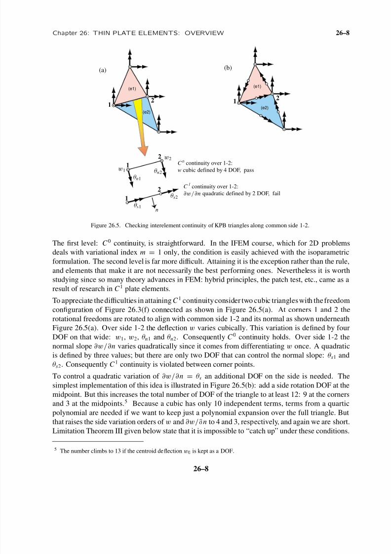
12 C continuity over 1-2:

quadratic defined by 2 DOF, fail

C continuity over 1-2:w cubic defined by 4 DOF, pass

1

0

∂w/∂ n

n

w1

w2

θn1

θn2

θs1

θs2

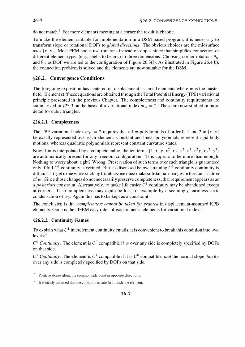
Figure 26.5. Checking interelement continuity of KPB triangles along common side 1-2.

The rst level: C 0 continuity, is straightforward. In the IFEM course, which for 2D problemsdeals with variational index m = 1 only, the condition is easily achieved with the isoparametricformulation. The second level is far more dif cult. Attaining it is the exception rather than the rule,and elements that make it are not necessarily the best performing ones. Nevertheless it is worthstudying since so many theory advances in FEM: hybrid principles, the patch test, etc., came as a

result of research in C 1

plate elements.To appreciate thedif culties in attaining C 1 continuityconsider two cubic triangleswith the freedomcon guration of Figure 26.3(f) connected as shown in Figure 26.5(a). At corners 1 and 2 therotational freedoms are rotated to align with common side 1-2 and its normal as shown underneathFigure 26.5(a). Over side 1-2 the de ection w varies cubically. This variation is de ned by fourDOF on that wide: w 1 , w 2 , θn1 and θn2 . Consequently C 0 continuity holds. Over side 1-2 thenormal slope ∂w/∂ n varies quadratically since it comes from differentiating w once. A quadraticis de ned by three values; but there are only two DOF that can control the normal slope: θs1 andθs2 . Consequently C 1 continuity is violated between corner points.

To control a quadratic variation of ∂w/∂ n = θs an additional DOF on the side is needed. The

simplest implementation of this idea is illustrated in Figure 26.5(b): add a side rotation DOF at themidpoint. But this increases the total number of DOF of the triangle to at least 12: 9 at the cornersand 3 at the midpoints. 5 Because a cubic has only 10 independent terms, terms from a quarticpolynomial are needed if we want to keep just a polynomial expansion over the full triangle. Butthat raises the side variation orders of w and ∂w/∂ n to 4 and 3, respectively, and again we are short.Limitation Theorem III given below state that it is impossible to “catch up ” under these conditions.

5 The number climbs to 13 if the centroid de ection w0 is kept as a DOF.

26– 8



26– 9 §26.3 *KINEMATIC LIMITATION PRINCIPLES

x

x

y

y

C

–

–

Pr

ϕ

s

s A

B

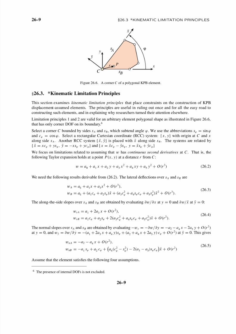
Figure 26.6. A corner C of a polygonal KPB element.

§26.3. *Kinematic Limitation Principles

This section examines kinematic limitation principles that place constraints on the construction of KPBdisplacement-assumed elements. The principles are useful in ruling out once and for all the easy road toconstructing such elements, and in explaining why researchers turned their attention elsewhere.

Limitation principles 1 and 2 are valid for an arbitrary element polygonal shape as illustrated in Figure 26.6,that has only corner DOF on its boundary. 6

Select a corner C bounded by sides s A and s B , which subtend angle ϕ. We use the abbreviations sϕ = sin ϕand cϕ = cos ϕ. Select a rectangular Cartesian coordinate (RCC) system: x , y with origin at C and xalong side s A . Another RCC system ¯ x , ¯ y is placed with ¯ x along side s B . The systems are related by ¯ x = xcϕ + ysϕ , ¯ y = − xsϕ + yc ϕ and x = xcϕ − ysϕ , y = x sϕ + yc ϕ

We focus on limitations related to assuming that w has continuous second derivatives at C . That is, thefollowing Taylor expansion holds at a point P ( x , y) at a distance r from C :

w = a 0 + a 1 x + a 2 y + a 3 x 2 + a 4 x y + a 5 y2 + O (r 3 ) ( 26 .2)

We need the following results derivable from (26.2). The lateral de ections over s A and s B are

w A = a 0 + a 1 x + a 3 x2 + O (r 3 ),

w B = a 0 + (a 1cϕ + a 2sϕ) ¯ x + (a 3c2ϕ

+ a 4sϕcϕ + a 5s 2ϕ

) ¯ x 2 + O (r 3 ).(26 .3)

The along-the-side slopes over s A and s B are obtained by evaluating ∂w/∂ x at y = 0 and ∂w/ ¯ x at ¯ y = 0:

w s A = a 1 + 2a 3 x + O (r 2 ),

w s B = a 1cϕ + a 2sϕ + 2(a 3c2ϕ

+ a 4sϕcϕ + a 5c2ϕ

) ¯ x + O (r 2 ).(26 .4)

The normal slopes over s A and s B are obtained by evaluating − w y = − ∂w/∂ y = − a 2 − a 4 x − 2a 5 y + O (r 2 )

at y = 0, and w ¯ y = ∂w/∂ ¯ y = − (a 1 + 2a 3 x + a 4 y)sϕ + (a 2 + a 4 x + 2a 5 y) cϕ + O (r 2

) at ¯ y = 0. This gives

w n A = − a 2 − a 4 x + O (r 2 ),

w nB = − a 1 sϕ + a 2 cϕ + a 4 (c2ϕ

− s 2ϕ

) − 2(a 3 − a 5)sϕcϕ ¯ x + O (r 2 )(26 .5)

Assume that the element satis es the following four assumptions.

6 The presence of internal DOFs is not excluded.

26– 9




(I) The Taylor series (26.2) at C is valid; thus the de ection w has second derivatives at C .

(II) Three nodal values are chosen at C : w C = a 0 , θ xC = (∂w/∂ y)C = a 1 and θ yC = − (∂w/∂ x )C = − a 2 .This is the standard choice for plate elements.

(III) Completeness is satis ed in that the six states w = 1, x , y, x 2 , x y, y2 are exactly representable overthe element.

(IV) The variation of the normal slope ∂w/∂ n along the element sides is linear.

§26.3.1. Limitation Theorem I

A KPB element cannot satisfy (I), (II), (III) and (IV) simultaneously.

Proof . Choose three set of corner DOF at C to satisfy:

Set 1: w C = 1,∂w∂n A C

= 0,∂w∂n B C

= 0,

Set 2: w C = 0,∂w∂n A C

= 1,∂w∂n B C

= 0,

Set 3: w C = 0,∂w∂n A C = 0,

∂w∂n B C = 1.

(26 .6)

while all other DOF are set to zero.

Set 1 imposes a 0 = 1 and a 1 = a 2 = 0. Both normal slopes at C are zero, and so are at other corners. Becauseof the linear variation assumption (IV), w n A = ∂w/∂ n A ≡ 0 and w nB = ∂w/∂ n B ≡= 0. Expressions (26.5)require a 4 = 0 and a 3 = a 5 .

Set 2 imposes a 0 = 0, a 1 = 1 and a 2 = cϕ / sϕ . Now w nB ≡ 0. This requires a 4 = 0 and a 3 = a 5 , as above.Replacing gives w n A = 1, which contradicts (IV).

Set 3 imposes a 0 = a 1 = 0, and a 2 = 1. Now w n A = 0 identically, which forces a 4 = 0.

An arbitrary set of values for the DOFs at C can be written as a linear combination of (26.6). But any suchcombination requires a 4 = 0, making the twist term vanish identically in (26.1). Thus the assumption (IV) of completeness cannot be satis ed.

Oddly enough the proof needs no assumption about how w varies along the sides; that is, C 0 compatibility.Just the assumption that the normal slope varies linearly is enough to kill completeness.

This theorem says that to get a C 1 compatible element while retaining assumptions (I), (II) and (III) the normalslope variation cannot be linear. Such conforming elements can be constructed, for example, using product of cubic Hermitian functions along side directions with sutable damping factors along the other directions. Butthis approach runs into serious trouble as shown by the next limitation principle.

§26.3.2. Limitation Theorem II

Any C 1-compatible, non rectangular KPB element that satis es conditions (I) and (II) cannot represent exactly

all constant curvature states.Proof . If the element is exactly in a constant curvature state, the de ection w must be quadratic in x , y.Hence the normal slope variation must be linear. But according to Limitation Theorem I the element cannotrepresent the constant twist state.

This theorem shows that (I), (II) and (III) are incompatible. A more detailed study shows that for a C 1

compatible rectangular element with sides aligned with x , y only the twist state is lost but that x2 and y2 canbe exactly represented. For non-rectangular geometries all constant curvature states are lost.

If one insists in C 1 continuity there are two ways out:

26– 10



26– 11 §26.3 *KINEMATIC LIMITATION PRINCIPLES

Abandon (I): Keep a single polynomial over the element but admit higher order derivatives as corner degreesof freedom.

Abandon (II): Permit discontinuous second derivatives at corners through the use of non-polynomial assump-tions, or macroelements.

Both techniques have been tried with success. The use of second derivatives as DOFs, if (I) is abandoned, is

forced by the next limitation principle.

§26.3.3. Limitation Theorem III

Suppose that a simple complete polynomial expansion of order n ≥ 3 is assumed for w over a triangle. Ateach corner i the de ection w i , the slopes w xi , w yi and all midsurface derivatives up to order m ≥ 1 are takenas degrees of freedom. Then C 1 continuity requires m ≥ 2 and n ≥ 5.

Proof . Proven in the writer ’s thesis. 7

Here is an informal summary of the proof. The total number of DOFs for a complete polynomial is Pn =(n + 1)( n + 2)/ 2 = F n + Bn . Of these F n = min (n + 1)( n + 2)/ 2, 6n − 9 are called fundamental freedoms

in the sense that they affect interelement compatibility. The Bn = max 0, ( n − 5)( n − 4)/ 2 are called bubble

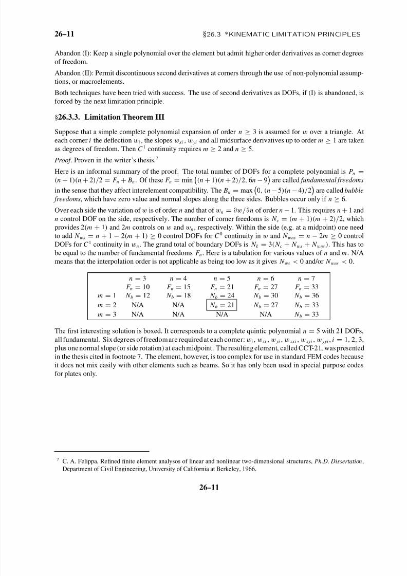
freedoms , which have zero value and normal slopes along the three sides. Bubbles occur only if n ≥ 6.Over each side the variation of w is of order n and that of w n = ∂w/∂ n of order n − 1. This requires n + 1 andn control DOF on the side, respectively. The number of corner freedoms is N c = (m + 1)( m + 2)/ 2, whichprovides 2 (m + 1) and 2 m controls on w and w n , respectively. Within the side (e.g. at a midpoint) one needto add N w s = n + 1 − 2(m + 1) ≥ 0 control DOFs for C 0 continuity in w and N w ns = n − 2m ≥ 0 controlDOFs for C 1 continuity in w n . The grand total of boundary DOFs is N b = 3( N c + N w s + N w ns ) . This has tobe equal to the number of fundamental freedoms F n . Here is a tabulation for various values of n and m . N/Ameans that the interpolation order is not applicable as being too low as it gives N w s < 0 and/or N w ns < 0.

n = 3 n = 4 n = 5 n = 6 n = 7F n = 10 F n = 15 F n = 21 F n = 27 F n = 33

m = 1 N b = 12 N b = 18 N b = 24 N b = 30 N b = 36m = 2 N/A N/A N b = 21 N b = 27 N b = 33m = 3 N/A N/A N/A N/A N b = 33

The rst interesting solution is boxed. It corresponds to a complete quintic polynomial n = 5 with 21 DOFs,all fundamental. Six degrees of freedomare requiredat each corner: w i , w xi , w yi , w xxi , w xyi , w yyi , i = 1, 2, 3,plus one normal slope (or side rotation) at eachmidpoint. The resulting element, called CCT-21, was presentedin the thesis cited in footnote 7. The element, however, is too complex for use in standard FEM codes becauseit does not mix easily with other elements such as beams. So it has only been used in special purpose codesfor plates only.

7 C. A. Felippa, Re ned nite element analysos of linear and nonlinear two-dimensional structures, Ph.D. Dissertation ,Department of Civil Engineering, University of California at Berkeley, 1966.

26– 11




§26.4. Early Work

By the late 1950s the success of the Finite Element Method with membrane problems (for example, for wingcovers and fuselage panels) led to high hopes in its application to plate bending and shell problems. Therst results were published by 1960. But until 1965 only rectangular models gave satisfactory results. Theconstruction of successful triangular elements to model plates and shells of arbitrary geometry proved moredif cult than expected. Early failures, however, led to a more complete understanding of the theoretical basisof FEM and motivated several advances taken for granted today.

The major source of dif culties in plates is due to stricter continuity requirements. The objective of attainingnormal slope interelement compatibility posed serious problems, documented in the form of Limitation The-orems in §26.3. By 1963 researchers were looking around “escape ways ” to bypass those problems. It wasrecognized that completeness, in the form of exact representation of rigid body and constant curvature modes,was fundamental for convergence to the analytical solution, a criterion rst enuncaite by Melosh. 8 The effectof compatibility violations was more dif cult to understand until the patch test came along.

§26.4.1. Rectangular Elements

The rst successful rectangular plate bending element was developed by Adini and Clough 9 . This elementhas 12 degrees of freedom (DOF). It used a complete third order polynomial expansion in x and y, alignedwith the rectangle sides, plus two additional x3 y and x y3 terms. The element satis es completeness as well astransverse de ection continuity but normal slope continuity is only maintained at the four corner points. Thesame element results from another expansion proposed by Melosh (1963 reference cited), which erroneouslystates that the element satis es C 1 continuity. The error was noted in subsquent discussion. 10 In 1961 Meloshhad proposed 11 had proposed a rectangular plate element constructed with beam-like edge functions dampedlinearly toward the opposite side, plus a uniform twisting mode. Again C 0 continuity was achieved but notC 1 except at corners.

Both of the foregoing elements displayed good convergence characteristics when used for rectangular plates.However thesearch fora compatible displacement eldwasunderway to try to achievemonotonicconvergence.A fully compatible 12-DOF rectangular element was apparently rst developed by Papenfuss in an obscure

reference.12

The element appears to have been rediscovered several times. The simplest derivation can becarried out with products of Hermite cubic polynomials, as noted below. Unfortunately the uniform twist stateis not include in the expansion and consequently the element fails the completeness requirement, convergingmonotonically to a zero twist-curvature solution: the right answer for the wrong problem.

In a brief but important paper, Irons and Draper 13 stressed the importance of completeness for uniform strainmodes (constant curvature modes in the case of plate bending). They proved that it is impossible to constructany polygonal-shape plate element with only 3 DOFs per corner and continuous corner curvatures that cansimultaneously maintain normal slope conformity and inclusion of the uniform twist mode. This negative

8 R. J. Melosh, Bases for the derivation of stiffness matrices for solid continua, AIAA J. , bf 1, 1631 –1637, 1963.9 A. Adini and R. W. Clough, Analysis of plate bending by the nite element method, NSF report for Grant G-7337, Dept.

of Civil Engineering, University of California, Berkeley, 1960. Also A. Adini, Analysis of shell structures by the niteelement method, Ph.D. Dissertation, Department of Civil Engineering, University of California, Berkeley, 1961.10 J. L. Tocher and K. K. Kapur, Comment on Melosh ’s paper, AIAA J. , 3, 1215 –1216, 1965.11 R. J. Melosh, A stiffness matrix for the analysis of thin plates in bending, J. Aero. Sci. , 28, 34 –42, 1961.12 S. W. Papenfuss, Lateral plate de ection by stiffness methods and application to a marquee, M. S. Thesis, Department

of Civil Engineering, University of Washington, Seattle, WA, 1959.13 B. M. Irons and K. Draper, Inadequacy of nodal connections in a stiffness solution for plate bending, AIAA J., 3, 965 –966,

1965.

26– 12



26– 13 §26.4 EARLY WORK

result, presented in §26.3 as Limitation Theorem II, effectively closed the door to the construction of theanalog of isoparametric elements in plate bending.

The construction of fully compatible polynomials expansions of various orders for rectangular shapes wassolved by Bogner et al in 1965 14 through Hermitian interpolation functions. In their paper they rederivedPapenfuss ’ element, but in an Addendum 15 they recognised the lack of the twist mode and an additional degree

of freedom: the twist curvature, was added at each corner. The 16-DOF element is complete and compatible,and produced excellent results. More re ned rectangular elements with 36 DOFs have been also developedusing fth order Hermite polynomials.

§26.4.2. Triangular Elements

Flat triangular plate elements have a wider range of application than rectangular elements since they naturallyconform to the analysis of plates and shells of arbitrary geometry for small and large de ections. But aspreviously noted the development of adequate kinematic expansions was not an easy problem and has keptresearchers busy for decades.

The success of incompatible rectangular elements is due to the fact that the assumed polynonial expansions forw can be considered as “natural ” deformation modes, after a trivial reduction to nondimensional form. They

are intrisically related to the geometry of the element because the local system is chosen along two preferreddirections. Lack of C 1 continuity between corners disppears in the limit of a mesh re nement.

Early attempts to construct triangular elements tried to mimic that scheme, using a RCC system arbitrarilyoriented with respect to the element. This lead to an unpleasant lack of invariance whenever an incompletepolynomial was selected, since kinematic constraints were arti cially imposed. Furthermore the role of completeness was not understood. Thus the rst suggested expansion for a triangular element with 9 DOFs 16

w = α 1 + α 2 x + α 3 y + α 4 x 2 + α 5 y2α 6 x 3 + α 7 x 2 y + α 8 x y2 + α 9 y3 (26 .7)

in which the x y term is missing, violates compability, completeness and invariance requirements. The elementconverges, but to the wrong solution with zero twist curvature.

Tocher in his thesis cited above tried two variants of the cubic expansion:

1 Combining the two cubic terms: x2 y + x y2 .

2 Using a complete 10-term cubic polynomial The rst choice satis es completeness but violates com-patibility and invariance. The second assumption satis es completeness and invariance but violatescompatibility and poses the problem: what to do with the extra DOF? Tocher decided to eliminate it by ageneralized inversion process, which unfortunately leads to discarding a fundamental degree of freedom.This led to an extremely exible (and non convergent) element. The elimination technique of Bazeleyet. al. discussed in Chapter 25 was more successful and produced an element which is still in use today.

The rst fully compatible 9-DOF cubic triangle was nally constructedby the macroelement technique. 17 . Thetriangle was divided into three subtriangles, over each of which a cubic expansion with linear variation along

14 F. K. Bogner, R. L. Fox and L. A. Schmidt Jr., The generation of interelement compatible stiffness and mass matricesby the use of interpolation formulas, Proc. Conf. on Matrix Methods in Structural Mechanics , WPAFB, Ohio, 1965, in

AFFDL TR 66-80 , pp. 397 –444, 1966.15 Addendum to aforementioned paper, 411 –413 in AFFDL TR 66-80 .16 J. L. Tocher, Analysis of plate bending using triangular elements, Ph. D. Dissertation , Dept. of Civil Engineering,

University of California, Berkeley, California, 1963.17 R. W. Clough and J. L. Tocher, Finite element stiffness matrices for analysis of plate bending, Proc. Conf. on Matrix

Methods in Structural Mechanics, WPAFB, Ohio, 1965, in AFFDL TR 66-80 , 515 –545, 1966.

26– 13




the exterior side was assumed. A similar element with quadratic slope variation and 12 DOF was constructedby the writer. 18 The original derivations, carried out in x , y coordinates were considerably simpli ed later byusing triangular coordinates.

The 1965 paper by Bazeley et al. 19 was an important milestone. In it three plate bending triangles weredeveloped. Two compatible elements were developed using rational functions. Experiments showed them to

be quite stiff and have no interest today. An incompatible element called the BCIZ triangle since was obtainedby eliminating the 10th DOF from a complete cubic in such as way that completeness was maintained. Thiselement is incompatible. Numerical experiments showed that it converged for some mesh patterns but not forothers. This puzzling behavior led to the invention of the patch test. 20 The patch test was further developedby Irons and coworkers in the 1970s. 21 A mathematical version is presented in the Strang-Fix monograph. 22

§26.4.3. Quadrilateral Elements

Arbitrary quadrilaterals can be constructed by assembling several triangles, and eliminating internal DOFs, if any by static condensation. This represents an ef cient procedure to take into account that the four cornersneed not be on a plane. The article by Clough and Felippa cited above presents the rst quadrilateral elementconstructed this way. That element was included in the open-source SAP family of FEM codes and used forshell analysis since 1968.

A direct construction of an arbitrary quadrilateral with 16 DOFs was presented by de Veubeke. 23 The quadri-lateral is formed by a macroassembly of four triangles by the two diagonals, which are selected as a skewCartesian coordinate system to develop the nite element elds.

§26.5. More Recent Work

The fully conforming elements developed in the mid 1960s proved “safe ” for FEM program users in thatconvergence could be guaranteed. Performance was another matter. Triangular elements proved to be ex-cessively stiff, particularly for high aspect ratios. A signi cant improvement in performance was achievedby Razzaque 24 who replaced the shape function curvatures with least-square- tted smooth functions. Thistechnique was later shown to be equivalent to the stress-hybrid formulation.

The rst application of mixed functionals to nite elements was actually to the plate bending problem. Her-rman 25 developed a mixed triangular model in which transverse displacements and bending moments are

18 R. W. Clough and C. A. Felippa, A re ned quadrilateral element for analysis of plate bending, Proc. 2nd Conf. on MatrixMethods in Structural Mechanics, WPAFB, Ohio, 1965, in AFFDL TR 69-23 , 1969

19 G. P. Bazeley, Y, K. Cheung, B. M. Irons and O. C. Zienkiewicz, Triangular elements in plate bending — conformingand nonconforming solutions, Proc. Conf. on Matrix Methods in Structural Mechanics, WPAFB, Ohio, 1965, in AFFDLTR 66-80 , pp. 547 –576, 1966.

20 Addendum to Bazeley et. al. paper cited above, pp. 573 –576 in AFFDL TR 66-80 .21 B. M. Irons and A. Razzaque, Experiences with the patch test for convergence of nite elements, in Mathematical

Foundations of the Finite Element Method with Applications to Partial Differential Equations , ed. by K. Aziz, Academic

Press, New York, 1972.B. M. Irons and S. Ahmad, Techniques of Finite Elements , Ellis Horwood Ltd, Chichester, England, 1980.22 G. Strang and G. Fix, An Analysis of the Finite Element Method , Prentice-Hall, Englewood Cliffs, N.J., 1973.23 B. Fraeijs de Veubeke, A conforming nite element for plate bending, Int. J. Solids Struct. , 4, 95 –108, 196824 A. Razzaque, Program for triangularbending elements withderivative smoothing, Int. J.Numer. Meth. Engrg. , 6,333 –343,

1973.25 L.R.Herrmann,A bendinganalysis forplates, in Proceedings1stConferenceon Matrix Methodsin StructuralMechanics ,

AFFDL-TR-66-80, Air Force Institute of Technology, Dayton, Ohio, 577 –604, 1966.

26– 14



26– 15 §26.5 MORE RECENT WORK

selected as master variables. A linear variation was assumed for both variables. This work was based onthe HR variational principle and included the transversal shear energy. The element did not perform well inpractice.

Successful plate bending elements have also been been constructed by Pian ’s assumed-stress hybrid method 26

The 9-dof triangles in this class are normally derived by assuming cubic de ection and linear slope variations

along the element sides, and a linear variation of the internal moment eld. Ef cient formulations of suchelements have been published. 27 Hybrid elements generally give better moment accuracy than conformingdisplacement elements. The derivation of these elements, however, is more involved in that it depends onnding equilibrium moments elds within the element, which is not a straightforward matter if the momentsvary within the element or large de ections are considered.

Much of the recent research on displacement-assumed models has focused on relaxing or abandoning theassumptions of Kirchhoff thin-plate theory. Relaxing these assumptions has produced elements based on theso-called discrete Kirchhoff theory. 28 In this method the primary expansion is made for the plate rotations.The rotations are linked to the nodal freedoms by introduction of thin-plate normality conditions at selectedboundary points, and then interpolating displacements and rotations along the boundary. The initial appli-cations of this method appear unduly complicated. A clear and relatively simple account is given by Batoz,Bathe and Ho. 29 The most successful of these elements to date is the DKT (Discrete Kirchhoff Triangle), anexplicit formulation of which has been presented by Batoz. 30

A more drastic step consists of abandoning the Kirchhoff theory in favor of the Reissner-Mindlin theory of moderately thick plates. The continuity requirements for the displacement assumption are lowered to C 0

(hence the name “C 0 bending elements ”), but the transverse shear becomes an integral part of the formulation.

Historically the rst fully conforming triangular plate elements were not Clough-Tocher ’s but C 0 elementscalled “facet ” elements that were derived in the late 1950s, although an account of their formulation was notpublished until 1965. 31 Facet elements, however, suffer from severe numerical problems for thin-plate andobtuse-angle conditions. The approach was revived later by Argyris et. al. 32 within the context of degenerated“brick ” elements.

Successful quadrilateral C 0 elements have been developed by Hughes, Taylor and Kanolkulchai, 33 Pugh,

26 T. H. H. Pian, Derivation of element stiffness matrices by assumed stress distributions, AIAA J. , 2, 1333 –1336, 1964. T.H. H. Pian and P. Tong, Basis of nite element methods for solid continua, Int. J. Numer. Meth. Engrg. , 1, 3–29, 1969.

27 O. C. Zienkiewicz, The Finite Element Method in Engineering Science , McGraw-Hill, New York, 3rd edn., 1977.D. J. Allman, Triangular nite elements for plate bending with constant and linearly varying bending moments, Proc.

IUTAM Conf. on High Speed Computing of Elastic Structures , Li ege, Belgium, 105 –136, 1970.

28 J. Stricklin, W. Haisler, P. Tisdale and R. Gunderson, A rapidly converging triangular plate bending element, AIAA J. , 7,180 –181, 1969. Also G. Dhatt, An ef cient triangular shell element, AIAA J. , 8, No. 11, 2100 –2102, 1970.

29 J. L. Batoz, K.-J. Bathe and Lee-Wing Ho, A study of three-node triangular plate bending elements, Int. J. Numer. Meth. Engrg. , 15 , 1771 –1812, 1980.

30J. L. Batoz, An explicit formulation for an ef cient triangular plate-bending element, Int. J. Numer. Meth. Engrg. , 18,1077 –1089, 1982.

31 R. J. Melosh, A at triangular shell element stiffness matrix, Proc. Conf. on Matrix Methods in Structural Mechanics,WPAFB, Ohio, 1965, in AFFDL TR 66-80 , 503 –509, 1966.

32 J. H. Argyris, P. C. Dunne, G. A. Malejannakis and E. Schelkle, A simple triangular facet shell element with applicationsto linear and nonlinear equilibrium and elastic stability problems, Comp. Meths. Appl. Mech. Engrg. , 11 , 215 –247, 1977.

33 T. J. R. Hughes, R. Taylor and W. Kanolkulchai, A simple and ef cient nite element for plate bending, Int. J. Numer. Meth. Engrg. , 11 , 1529 –1543, 1977.

26– 15




Hinton and Zienkiewicz, 34 MacNeal, 35 Cris eld, 36 Tessler and Hughes, 37 Dvorkin and Bathe, 38 and Park andStanley. 39

Triangular elements in this class have been presented by Belytschko, Stolarski and Carpenter. 40 The construc-tion of robust C 0 bending elements is delicate, as they are susceptible to ‘shear locking ’ effects in the thin-plateregime if fully integrated, and to kinematic de ciencies (spurious modes) if they are not. When the proper

care is exercised good results have been reported for quadrilateral elements and, more recently, for triangularelements. 41

A different path has been taken by Bergan and coworkers, who retained the classical Kirchhoff formulationbut in conjunction with the use of highly nonconforming ( C − 1) shape functions. They have shown thatinterelement continuity is not an obstacle to convergence provided the shape functions satisfy certain energyand force orthogonality conditions 42 or the stiffness matrix is constructed using the free formulation 43 ratherthan the standard potential energy formulation. A characteristic feature of these formulations is the carefulseparation between basic and higher order assumed displacement functions or “modes ”. Results for triangularbending elements derived through this approach have reported satisfactory performance. 44 One of theseelements, which is based on force-orthogonal higher order functions, was rated in 1983 as the best performerin its class. 45

34 E. D. Pugh, E. Hinton and O. C. Zienkiewicz, A study of quadrilateral plate bending elements with reduced integration, Int. J. Numer. Meth. Engrg. , 12, 1059 –1078, 1978.

35 R. H. MacNeal, A simple quadrilateral shell element, Computers & Structures , 8, 175 –183, 1978.R. H. MacNeal, Derivation of stiffness matrices by assumed strain distributions, Nucl. Engrg. Design , 70, 3–12, 1982.

36 M. A. Cris eld, A four-noded thin plate bending element using shear constraints – a modi ed version of Lyons ’ element,Comp. Meths. Appl. Mech. Engrg. , 39, 93 –120, 1983.

37 A. Tessler and T. J. R. Hughes, A three-node Mindlin plate element with improved transverse shear, Comp. Meths. Appl. Mech. Engrg. , 50 , 71 –101, 1985.

38 E. N. Dvorkin and K. J. Bathe, A continuum mechanics based four-node shell element for general nonlinear analysis, Engrg. Comp. , 1, 77 –88, 1984.

39 G. M. Stanley, Continuum-based shell elements, Ph. D. Dissertation , Department of Mechanical Engineering, StanfordUniversity, 1985.K. C. Park and G. M. Stanley, A Curved C 0 shell element based on assumed natural-coordinate strains, J. Appl. Mech. ,108 , 278 –286, 1986.

40 T. Belytschko, H. Stolarski and N. Carpenter, A C 0 triangular plate element with one-point quadrature, Int. J. Numer. Meth. Engrg. , 20 , 787 –802, 1984.

41 A. Tessler and T. J. R. Hughes, A three-node Mindlin plate element with improved transverse shear, Comp. Meths. Appl. Mech. Engrg. , 50 , 71 –101, 1985.

42 P. G. Bergan, Finite elements based on energy-orthogonal functions, Int. J. Numer. Meth. Engrg. , 11 , 1529 –1543, 1977.43 P. G.Bergan and M.K. Nyg ard, Finite elements with increased freedomin choosing shape functions, Int. J. Numer. Meth.

Engrg. , 20 , 643 –664, 1984.

44 P. G. Bergan and L. Hanssen, A new approach for deriving “good ” nite elements, MAFELAP II Conference, BrunelUniversity, 1975, in The Mathematics of Finite Elements and Applications – Vol. II , ed. by J. R. Whiteman, AcademicPress, London, 1976. L. Hanssen, T. G. Syvertsen and P. G. Bergan, Stiffness derivation based on element convergencerequirements, MAFELAP III Conference, Brunel University, 1978, in The Mathematics of Finite Elements and Applica-tions – Vol III , ed. by J. R. Whiteman, Academic Press, London, 1979. P. G. Bergan and M. K. Nyg ard, Nonlinear shellanalysis using free formulation nite elements, Proc. Europe-US Symposium on Finite Element Methods for Nonlinear Problems , Springer-Verlag, 1986.

45 B. M. Irons, Putative high-performance plate bending element, Letter to Editor, Int. J. Numer. Meth. Engrg. , 19, 310,1983.

26– 16

Documents

Plate Element2