1 Phenotypic Fluctuation (Plasticity) vs Evolution2 Phenotypic Fluctuation vs Genetic Variation3 Evolution of Robustness to Noise and to Mutation4 Plasticity of each phenotype5 Restoration of Plasticity6 LeChatlier Principle? 7 Symbiotic Sympatric Speciation8 Evolution of Morphogenesis

selection of dynamical systems by dynamical systems for dynamical systems

Darwin and Lincoln (born on the same day)

Plasticity and Robustness in Evolution: Macroscopic Theory, Model Simulations, and Laboratory Experiments

Kunihiko Kaneko U Tokyo,Center for Complex Systems Biology

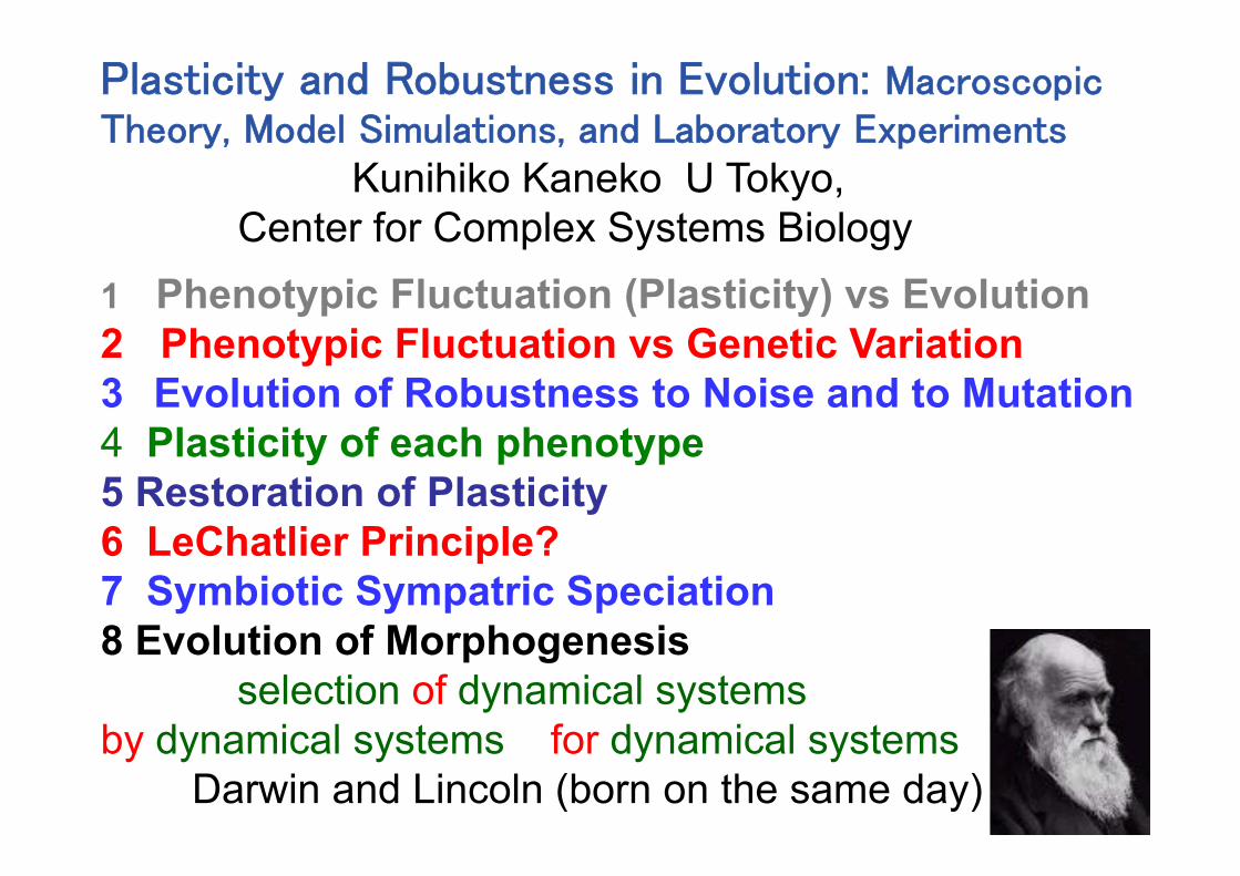
Adaptation asa result of consistencybetween cell growth andgene expression dynamics

Consistency between Multicelluar developmentand cell reprodcution

Genotype

Catalytic reaction network

Phenotype

Evolutionary relationship on Robustness and Fluctuation

Gene regulationnetwork

Molecule

Cell

Multicelluarity

Ecosystem

Stochsatic dynamics

Complex-Systems Biology : Consistency between different levels as guiding principle

Consistency between Cell reproductionand molecule replication

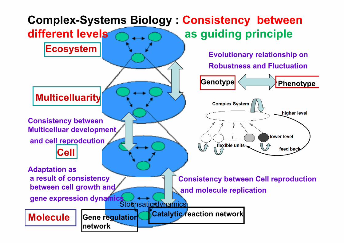
Consistency between dynamics of different levels

(1)Cell reproduction vs molecule replication adapt to critical state with optimal growth (Furusawa,kk PRL 03,12)(2) Cell Growth vs Protein Expression generic adaptation (without signal network) as a result of cell growth + noise (Kashiwagi etal,PLosOne 06)

(3) Cell reproduction vs multicellularity(unstable) oscillatory dynamics = stem cell + cell

interaction differentiation, loss of pluripotency(KK&Yomo 1997, Furusawa&KK,Science 2012)+ minimal model (Goto, kk, arXiv)

(4) Genetic vs phenotypic changes Today’s talk

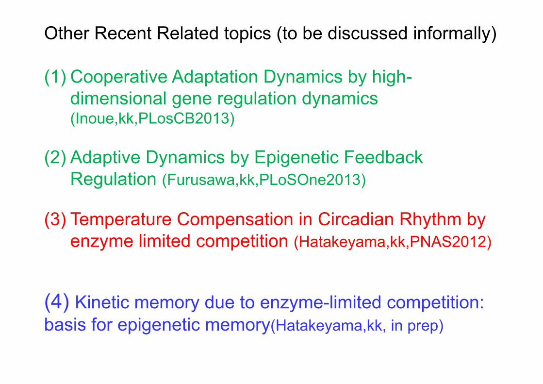
Other Recent Related topics (to be discussed informally)

(1) Cooperative Adaptation Dynamics by high-dimensional gene regulation dynamics (Inoue,kk,PLosCB2013)

(2) Adaptive Dynamics by Epigenetic Feedback Regulation (Furusawa,kk,PLoSOne2013)

(3) Temperature Compensation in Circadian Rhythm by enzyme limited competition (Hatakeyama,kk,PNAS2012)

(4) Kinetic memory due to enzyme-limited competition: basis for epigenetic memory(Hatakeyama,kk, in prep)

• Evolvability,Robustness,Plasticity: Basic Questions in Biology, but often discussed qualitatively : Idealizing the situation: quantitative theory?• Phenotypic Fluctuation

Phenotypic Evolution?• Even in isogenic individualslarge phenotypic fluctuation（theory, experiments)

• Motivation1 Relevance of this fluctuation to evolution?Positive role of noise?

Phenotypic fluctuation in EvoDevogenotype —``development ‘’ Phenotype Selection by f(Phenotype)（given environment)If this genotypephenotype mapping is uniquely determined selection by ｆ(Genotype). ThenChange in distribution P(genotype)

But gene—``development ‘’ Phenotype distributedPhenotypic fluctuation of isogenic organisms

P(x; a) x—phenotype, a – gene*Even if fluctuated phenotype is not heritable, degree of

fluctuation depends on gene and is heritableCorrespondence between Devo and Evocongruence between dev dynamics &evolution

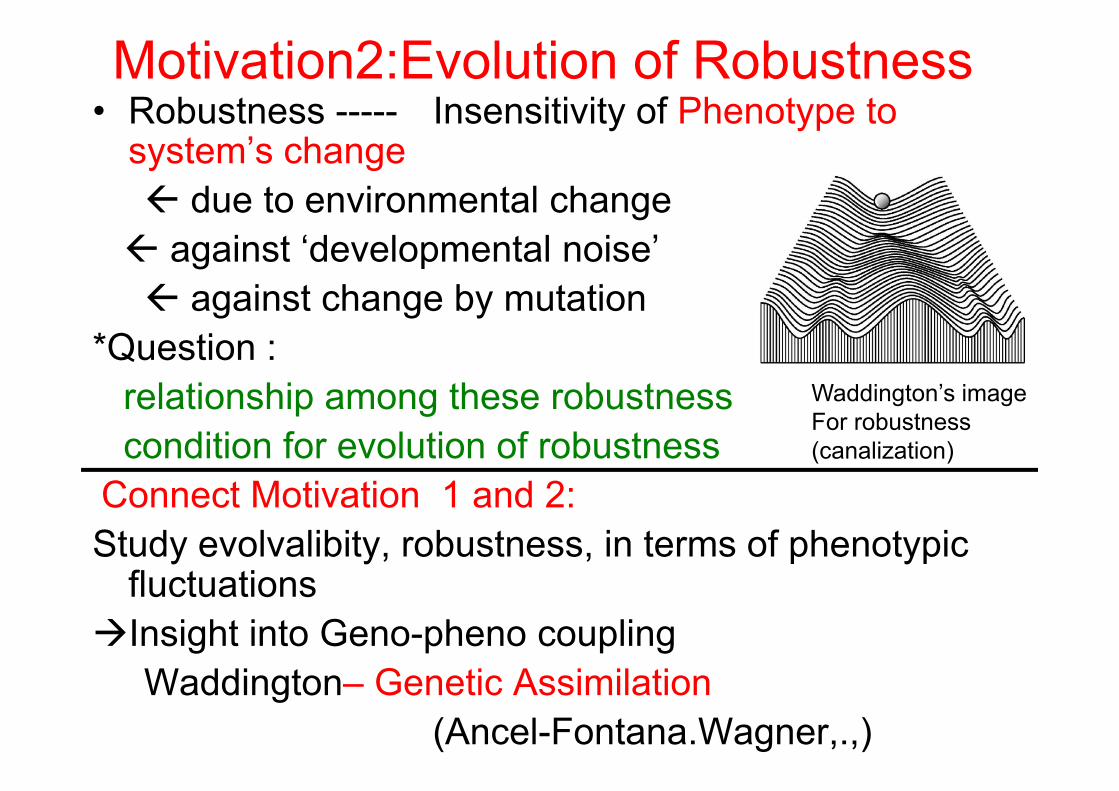
Motivation2:Evolution of Robustness• Robustness ----- Insensitivity of Phenotype to

system’s change due to environmental change against ‘developmental noise’ against change by mutation

*Question :relationship among these robustnesscondition for evolution of robustness

Connect Motivation 1 and 2:Study evolvalibity, robustness, in terms of phenotypic

fluctuationsInsight into Geno-pheno coupling

Waddington– Genetic Assimilation(Ancel-Fontana.Wagner,.,)

Waddington’s imageFor robustness(canalization)

• Note;phenomenological theory for relation betweenstochasticity in geno—pheno mappings andgenetic variances, based on Lab+Numericalexperiments+ phenomenological argument;

No sophisticated framework as in population genetics( cf: consequence of covariances is established

in Price, Lande,…..) Here, consequence of evo-devo (plasticity, robustness)

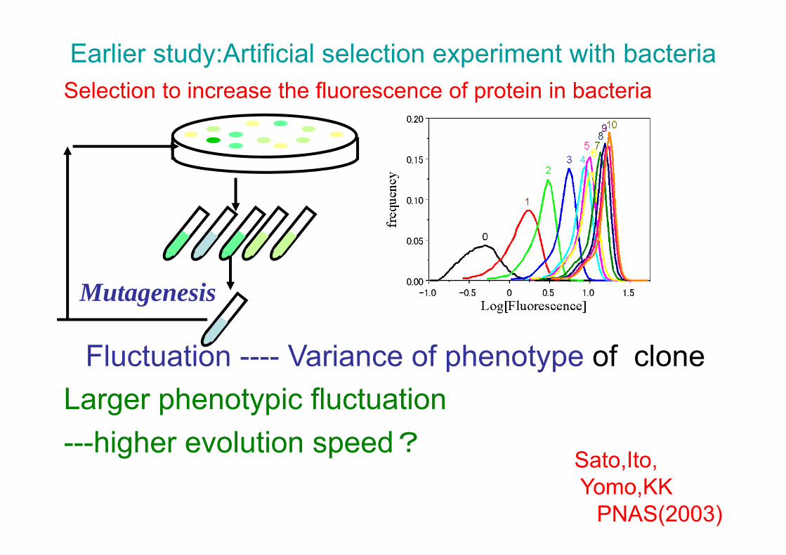
Fluctuation ---- Variance of phenotype of clone Larger phenotypic fluctuation ---higher evolution speed？

Earlier study:Artificial selection experiment with bacteriaSelection to increase the fluorescence of protein in bacteria

Mutagenesis

Sato,Ito,Yomo,KK

PNAS(2003)

Analogy with fluctuation-response relationshipForce to change a variable x;

response ratio = (shift of x ) / forcefluctuation of x (without force)

response ratio proportional to fluctuation

2 2( ) ( )a a aa

x x x x xa

P(x;a) x variable, a: control parameterchange of the parameter a

peak of P(x;a) ( i.e.,<x>average ) shifts

Generalization::(mathematical formulation)response ratio of some variable x against the change

of parameter a versus fluctuation of x

--``Response against mutation+selection’’ --Fluctuation

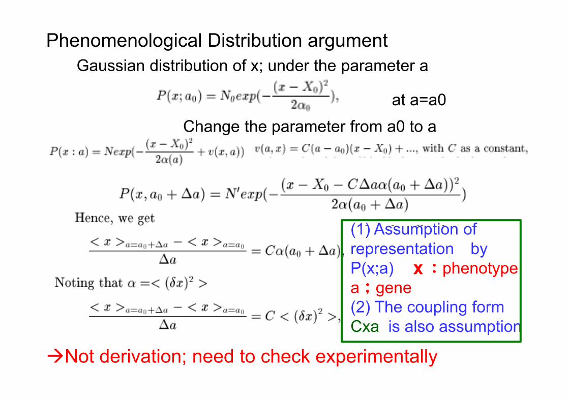
Phenomenological Distribution argumentGaussian distribution of x; under the parameter a

at a=a0Change the parameter from a0 to a

(1) Assumption of representation byP(x;a) ｘ：phenotypea；gene(2) The coupling form Cxa is also assumption

Not derivation; need to check experimentally

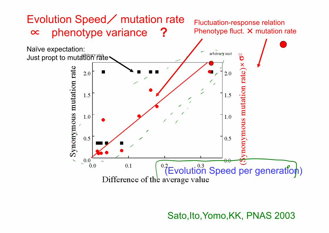
(Evolution Speed per generation)

Naïve expectation:Just propt to mutation rate

Fluctuation-response relationPhenotype fluct. × mutation rate

Sato,Ito,Yomo,KK, PNAS 2003

Evolution Speed／ mutation rate ∝ phenotype variance ？

• Confirmation by models

Requirement for modelsGenotype – rule for dynamics ( networks + parameters)Dynamics – high-dimensional (many degrees,e.g., expressions of proteins) + noisePhenotypes are shaped by attractor of the dynamical systemFitness (Phenotype) (high-fitness state is rare)Mutation+Selection process

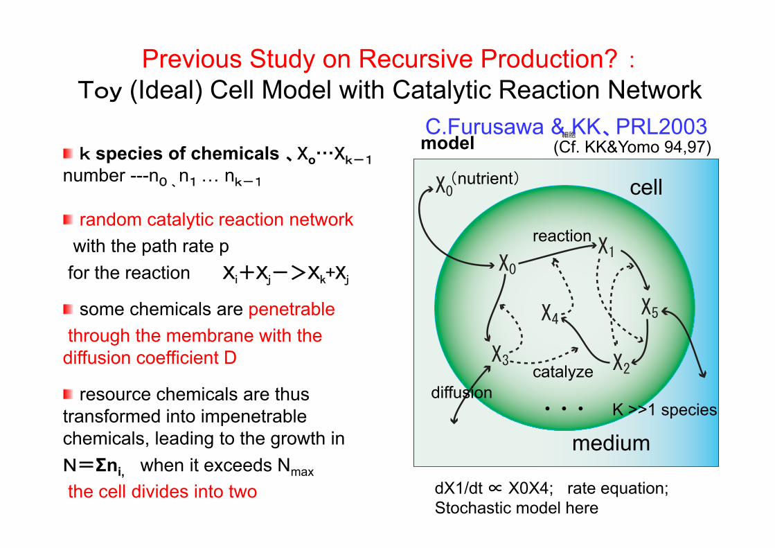
Previous Study on Recursive Production? ：Ｔｏｙ (Ideal) Cell Model with Catalytic Reaction Network

（nutrient）

reaction

catalyze

cell

medium

diffusion

ｋ species of chemicals 、Xo…Xｋ－１

number ---n０ 、n１ … nｋ－１

some chemicals are penetrablethrough the membrane with the diffusion coefficient D

resource chemicals are thus transformed into impenetrable chemicals, leading to the growth inＮ＝Σni, when it exceeds Nmax

the cell divides into two

random catalytic reaction networkwith the path rate p

for the reaction Ｘi＋Ｘj－＞Ｘk+Xj

modelC.Furusawa & KK、PRL2003

・・・ K >>1 species

dX1/dt ∝ X0X4; rate equation;Stochastic model here

(Cf. KK&Yomo 94,97)

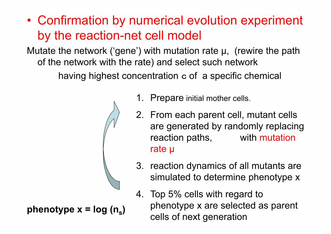
• Confirmation by numerical evolution experiment by the reaction-net cell model

Mutate the network (‘gene’) with mutation rate μ, (rewire the path of the network with the rate) and select such network

having highest concentration ｃ of a specific chemical

1. Prepare initial mother cells.

2. From each parent cell, mutant cells are generated by randomly replacing reaction paths, with mutation rate μ

3. reaction dynamics of all mutants are simulated to determine phenotype x

4. Top 5% cells with regard to phenotype x are selected as parent cells of next generation

phenotype x = log (ns)

Confirmation of Fluctuation Response Relationship by reaction-network cell model

Furusawa,KK 2005

μ=0.010.03

.0.05

Fluctuation of x=log c

Increase in average x

☆Growth speed and fidelity in replication are maximum at Dc

0.00

0.05

0.10

0.15

0.20

0.001 0.01 0.1 0

0.2

0.4

0.6

0.8

1

grow

th sp

eed

(a.u

.)

simila

rity

H

diffusion coefficient D

growth speedsimilarity

D = Dc

※similarity is defined from inner products of composition vectors between mother and daughter cells

・

・

DDc

No Growth

(only nutrients)

Growth

Remarks on the Catalytic Reaction Network Model

By tuning the flow rate to stay an optimal growthUniversal statistical law is observed ni (number of molecules

rank

Furusawa &KK,2003,PRL

Average number of each chemical ∝ 1/(its rank)

number rankX1 300 5X2 8000 1X3 5000 2X4 700 4X5 2000 3…….. (for example)

Power Law in Abundances of Chemicals

Human kidney, mouse ES yeast

Theory;To keep reproductionpreserving compositions

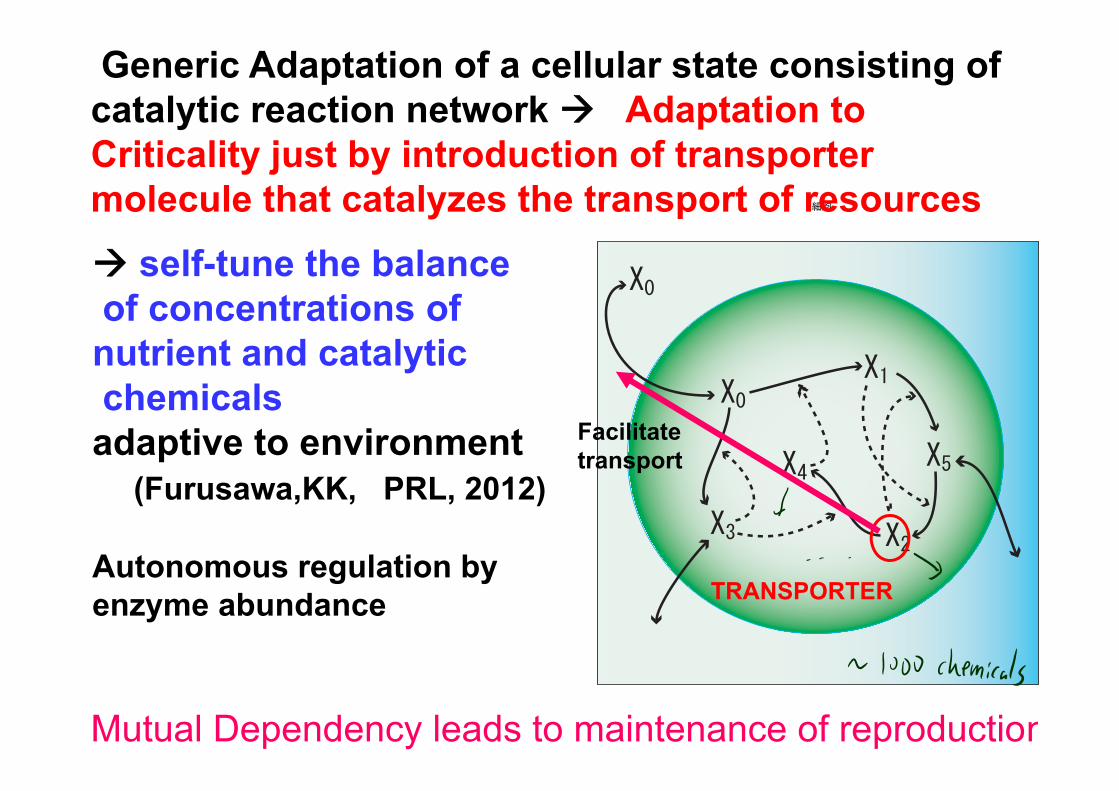
TRANSPORTER

Facilitatetransport

self-tune the balanceof concentrations of nutrient and catalyticchemicalsadaptive to environment

(Furusawa,KK, PRL, 2012)

Autonomous regulation by enzyme abundance

Generic Adaptation of a cellular state consisting of catalytic reaction network Adaptation to Criticality just by introduction of transporter molecule that catalyzes the transport of resources

Mutual Dependency leads to maintenance of reproduction

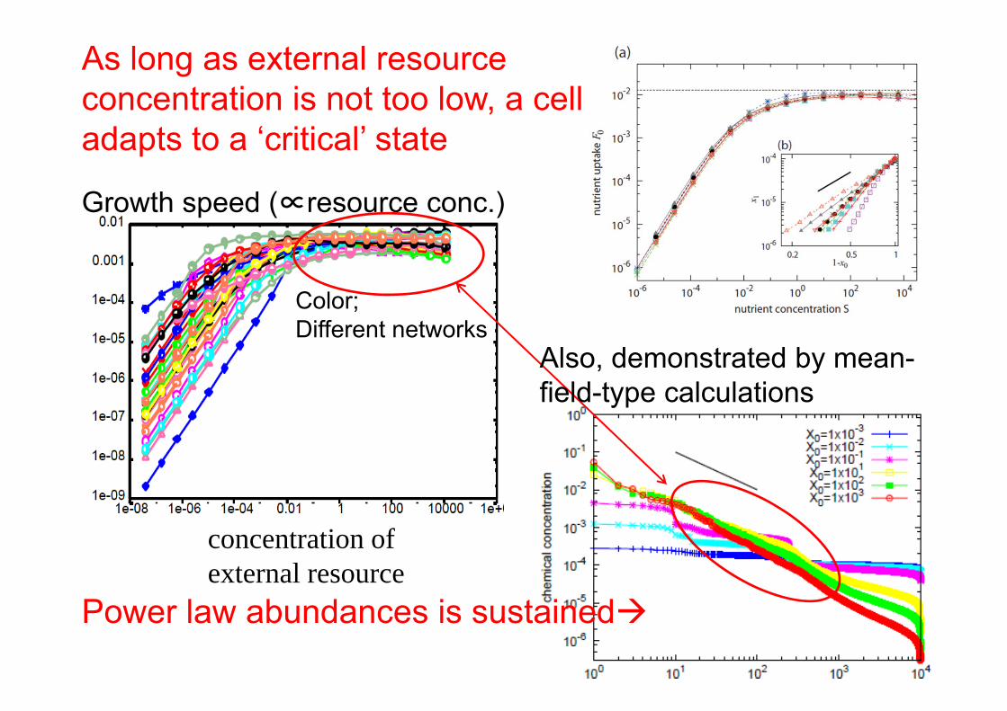
concentration of external resource

Growth speed (∝resource conc.)

Color;Different networks

As long as external resource concentration is not too low, a cell adapts to a ‘critical’ state

Power law abundances is sustained

Also, demonstrated by mean-field-type calculations

Change in environment (Resource )Adaptive dynamics (growth speed first changes and returns to the original

Adaptation dynamics (Fold Change Detection )

Fold-change detection: The adaptive dynamics depends only on the ratio of resources before and after. e.g., after change ofexternal resources100 200, 200 400,400 800 , identical dynamicscommon in present cells(Goentro-Kirschner, Alon et al,

Shimizu, Kamino-Sawai,…2009--),

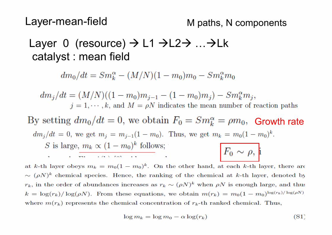
Layer 0 (resource) L1 L2…Lk catalyst : mean field

M paths, N components

Growth rate

log10(Xresponse / Xinitial)

log10(Xadapt /X

initial )All of 10000 chemicals ishow imperfect adaptation.Response/AdaptRi= C * Ai with 1> C>0

Ri

Ai

-1

~.7

Common High-dimensional Adaptation dynamicsall chemicals show ‘partial’ adaptation

Yeast, change in expression level of each gene by environmental change

RiAi

or

Log-scale

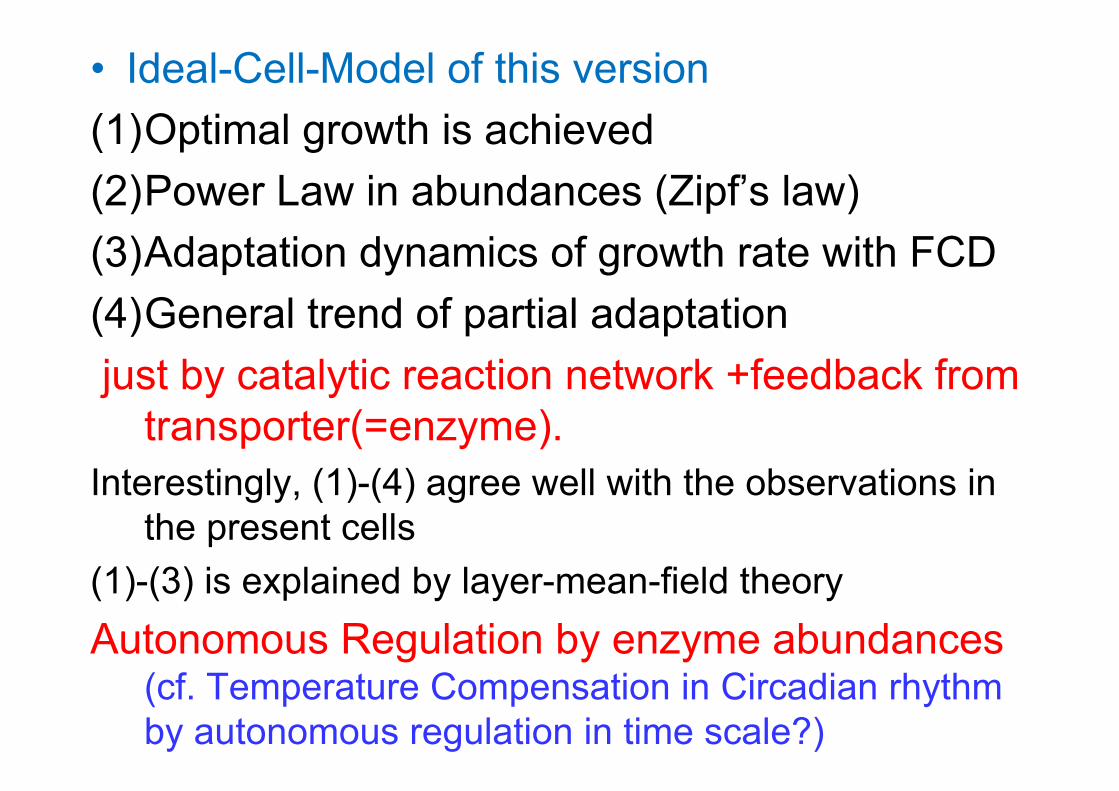
• Ideal-Cell-Model of this version(1)Optimal growth is achieved(2)Power Law in abundances (Zipf’s law)(3)Adaptation dynamics of growth rate with FCD(4)General trend of partial adaptationjust by catalytic reaction network +feedback from

transporter(=enzyme). Interestingly, (1)-(4) agree well with the observations in

the present cells(1)-(3) is explained by layer-mean-field theoryAutonomous Regulation by enzyme abundances

(cf. Temperature Compensation in Circadian rhythm by autonomous regulation in time scale?)

Confirmation of Fluctuation Dissipation Theorem by reaction-network cell model

Furusawa,KK 2005

μ=0.010.03

.0.05

Fluctuation of x=log c

Increase in average x

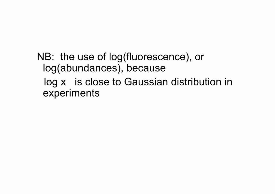
NB: the use of log(fluorescence), or log(abundances), becauselog x is close to Gaussian distribution in experiments

So far： Variance of Phenotype over Isogenic IndividualsVip ∝ Evolution Speed

Harder to evolve as development is rigid• ？Further Mystery？ Fundamental Theorem of Natural

Selection• Evolution speed∝ Variance of Average Phenotype over

heterogenic distribution Vg• （Fisher,established）： Then Vip ∝Vg？？

Gene distribution

phenotype

Isogenic individuals

phenotype

VipVg

a

x x（Vnoise or Ve）

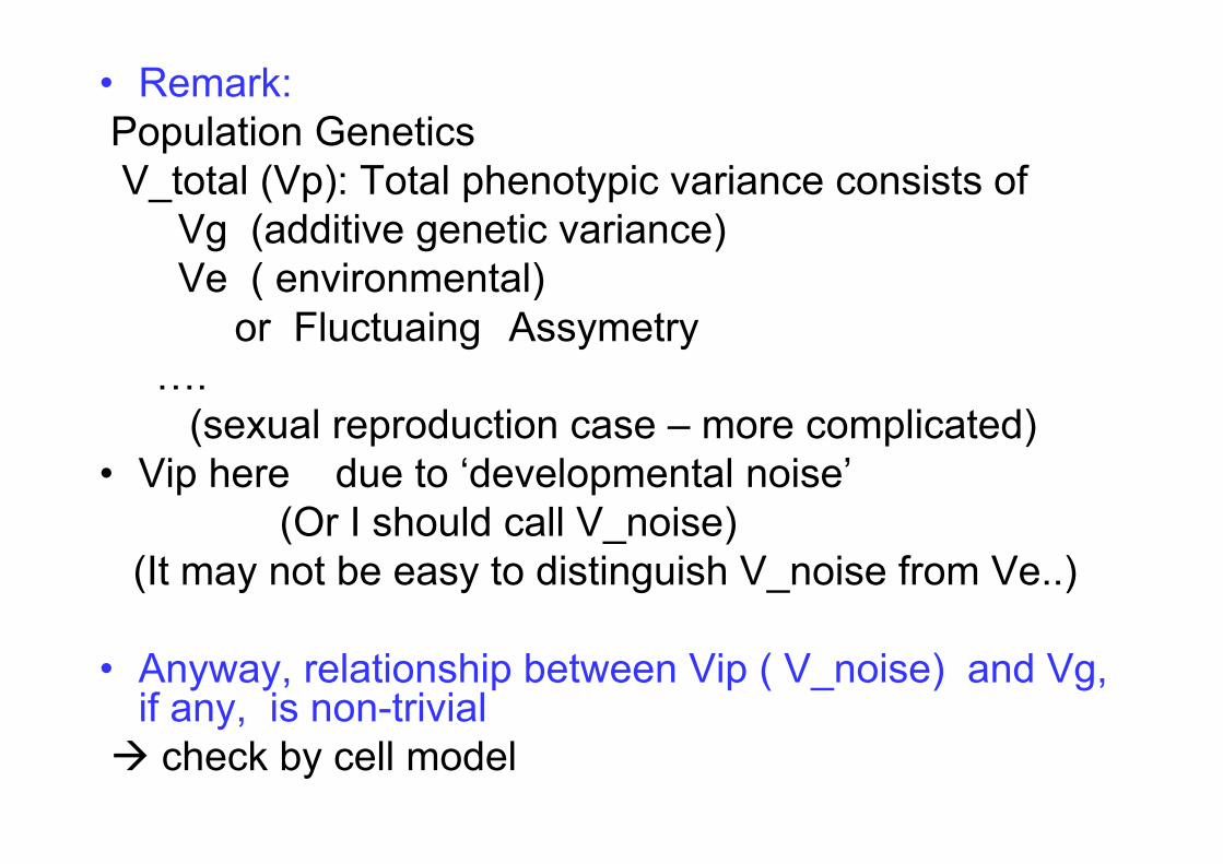
• Remark:Population GeneticsV_total (Vp): Total phenotypic variance consists of

Vg (additive genetic variance)Ve ( environmental)

or Fluctuaing Assymetry….

(sexual reproduction case – more complicated)• Vip here due to ‘developmental noise’

(Or I should call V_noise)(It may not be easy to distinguish V_noise from Ve..)

• Anyway, relationship between Vip ( V_noise) and Vg, if any, is non-trivial check by cell model

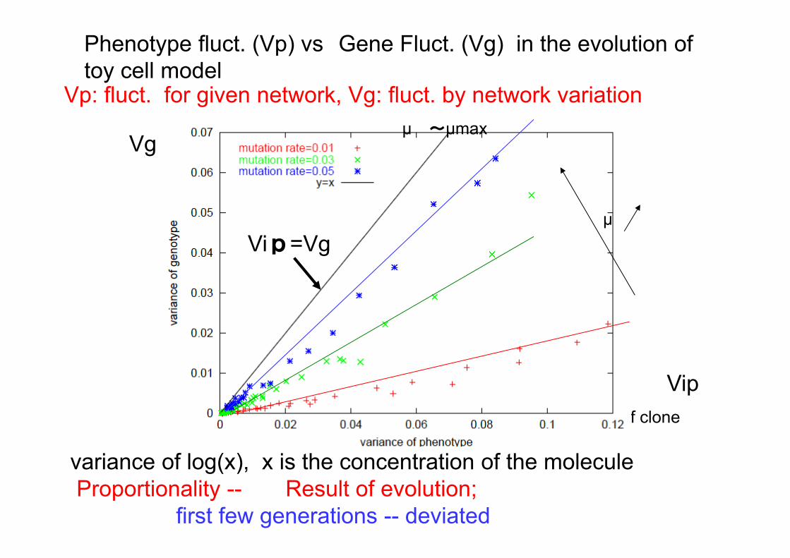
Phenotype fluct. (Vp) vs Gene Fluct. (Vg) in the evolution of toy cell model

VipPhenotype fluctuation of clone

variance of log(x), x is the concentration of the molecule Proportionality -- Result of evolution;

first few generations -- deviated

Vp: fluct. for given network, Vg: fluct. by network variation μ ～μmax

μViｐ=Vg

Vg

iip

Vip

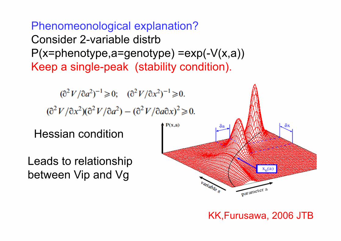
Phenomeonological explanation?Consider 2-variable distrbP(x=phenotype,a=genotype) =exp(-V(x,a))Keep a single-peak (stability condition).

Hessian condition

Leads to relationship between Vip and Vg

KK,Furusawa, 2006 JTB

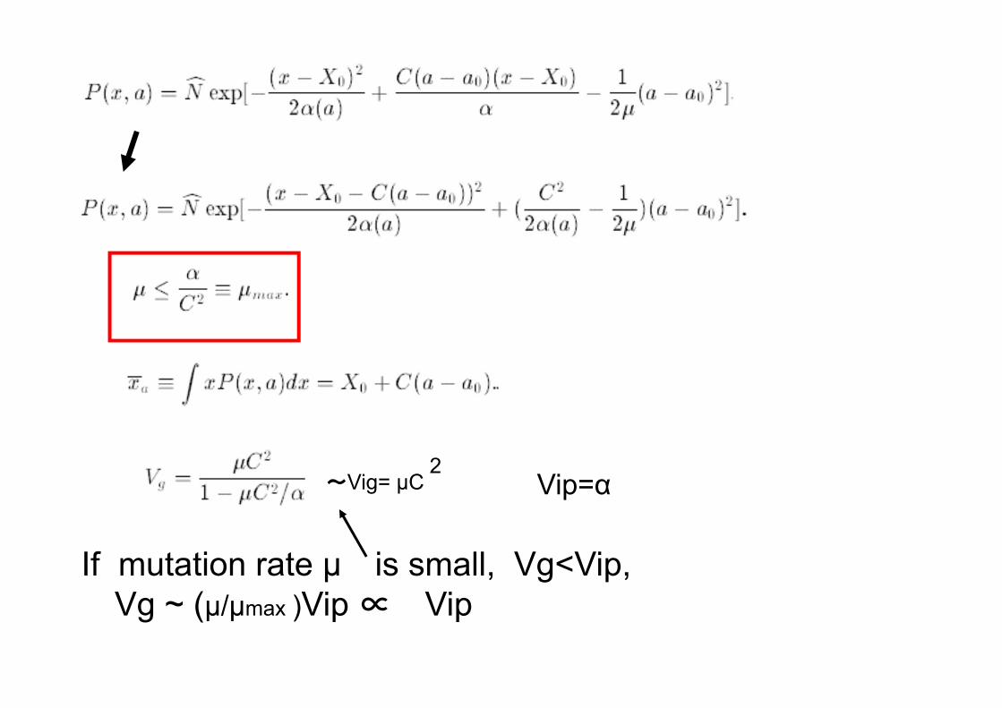
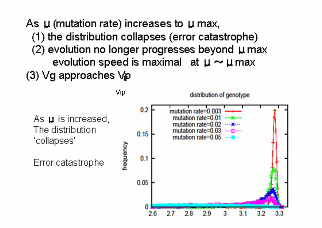
If mutation rate μ is small, Vg<Vip,Vg ~ (μ/μmax )Vip ∝ Vip

Vip=α～Vig= μC2

(i) Vip ≧ Vg （from stability condition) (under strong selection pressure) ( **)(ii)error catastrophe at Vip ~ Vg (**)

(where the evolution does not progress) (iii) Vg~(μ/μmax)Vip∝μVip

（∝evolution speed) at least for small μ＊＊Consistent with the experiments, but,,,,,Existence of P(x,a)?;+ Robust Evolution? +Why isogenetic phenotypic fluctuation leads to

robust evolution?(**) to be precisely Vig, variance those from a given phentype x: but Vig ~Vg if μ is small

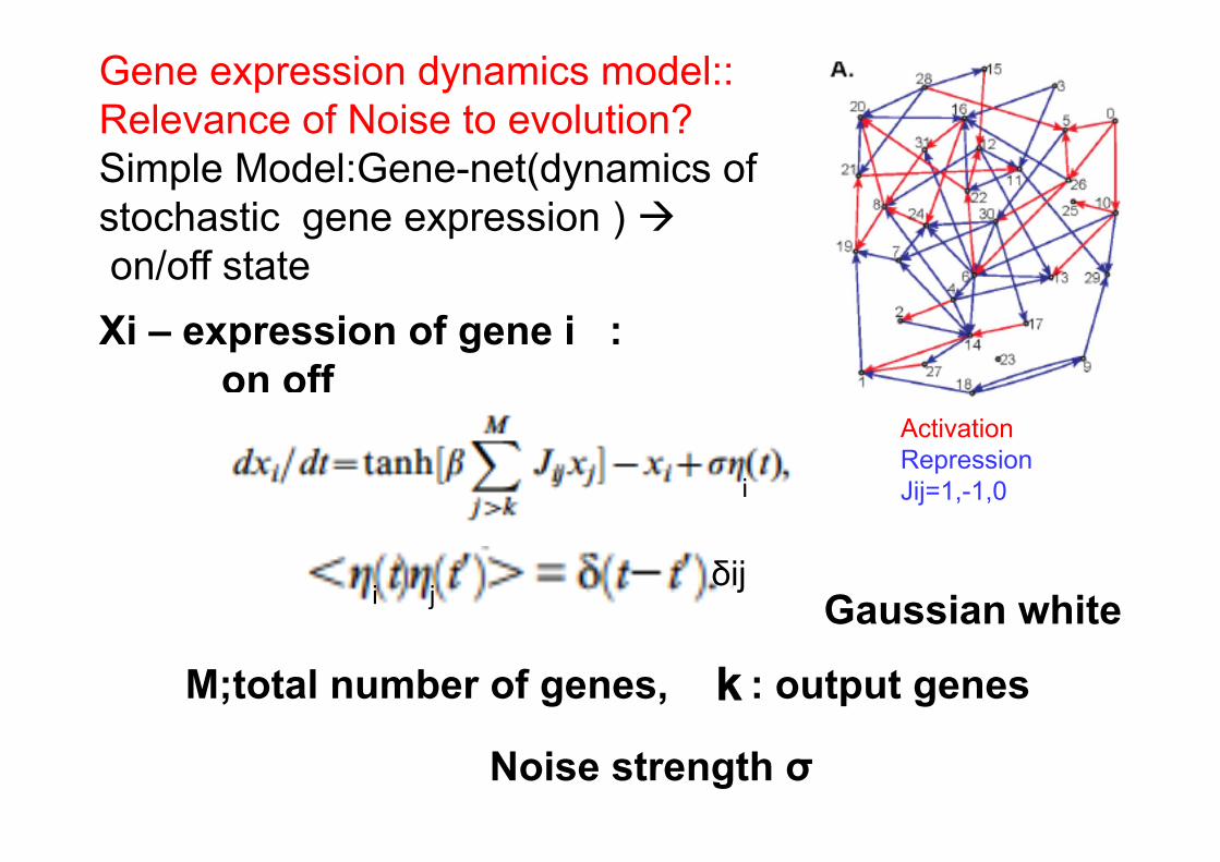
Gene expression dynamics model:: Relevance of Noise to evolution?Simple Model:Gene-net(dynamics of stochastic gene expression ) on/off stateXi – expression of gene i :

on off

i jδij

ActivationRepressionJij=1,-1,0

M;total number of genes, ｋ: output genes

Gaussian white

Noise strength σ

i

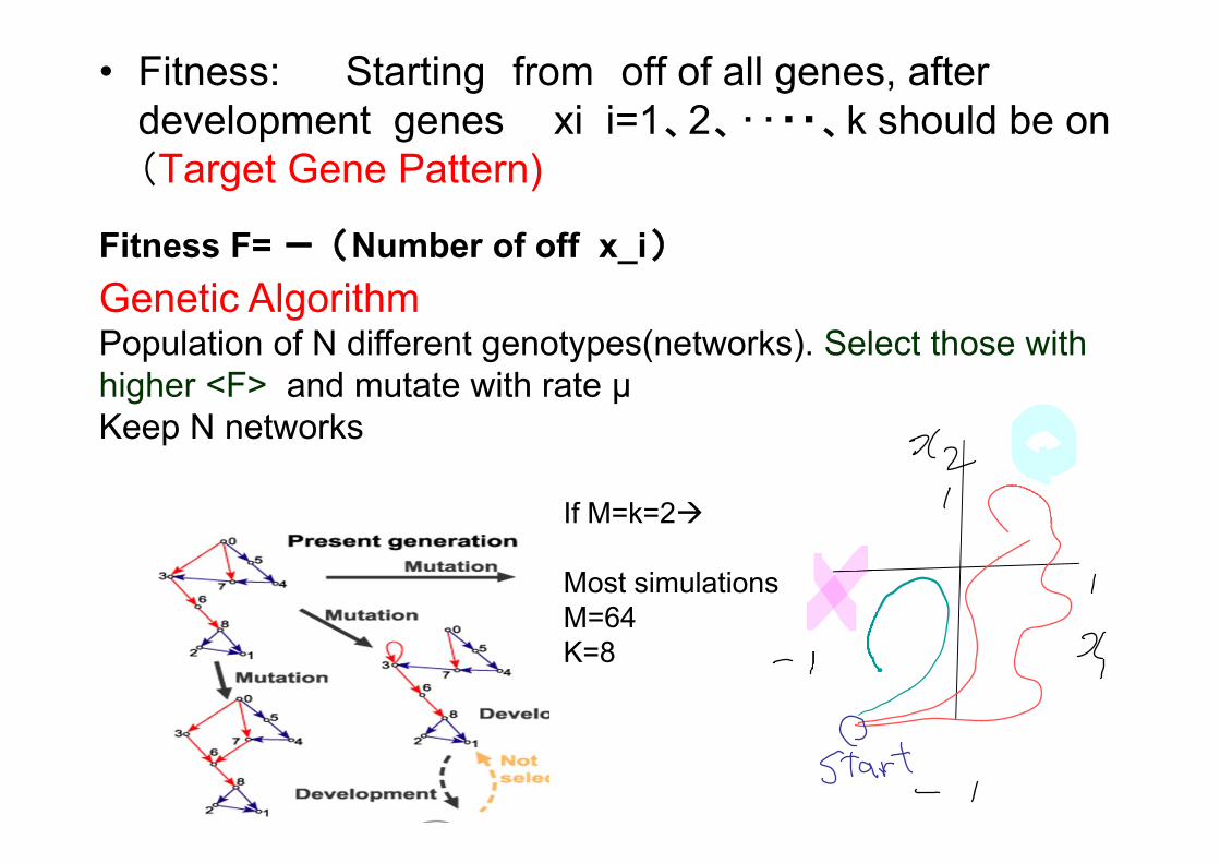
• Fitness: Starting from off of all genes, after development genes xi i=1、2、‥・・、k should be on（Target Gene Pattern)

Fitness F= －（Number of off x_i）Genetic AlgorithmPopulation of N different genotypes(networks). Select those with higher <F> and mutate with rate μKeep N networks

If M=k=2

Most simulationsM=64K=8

• Fitness increasesIsogenic Phenotypic Variance of decreases by generations through evolution

Variance ∝ evolution speedthrough generations

Results of Evolution Simulation （noise σ=.08)

Generation

Fitness

Evolution speed= Incrementof Fitness per generations

Variance

Top among existing networks (genotypes)

Lowest amonggenotypes

generation

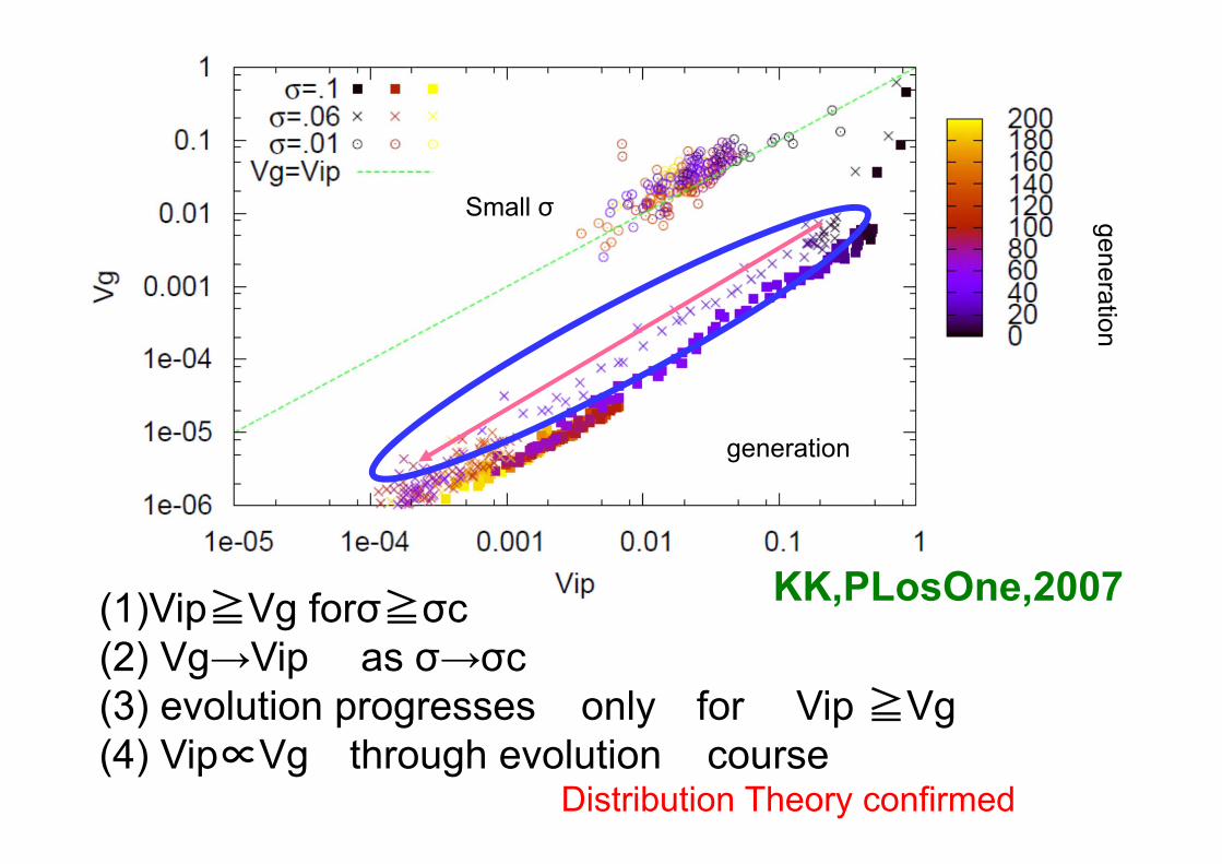
(1)Vip≧Vg forσ≧σc (2) Vg→Vip as σ→σc (3) evolution progresses only for Vip ≧Vg(4) Vip∝Vg through evolution course

Distribution Theory confirmed

KK,PLosOne,2007

Small σ

generation

This Vg-Vip relation is valid in the evolution under noisehigh noise( ) all (including mutants) reach the fittest

lower noise( ) non-fit mutants remain

Low Noise case High Noise case

Top among existing networks (genotypes)

Lowest amonggenotypes

GenerationGeneration

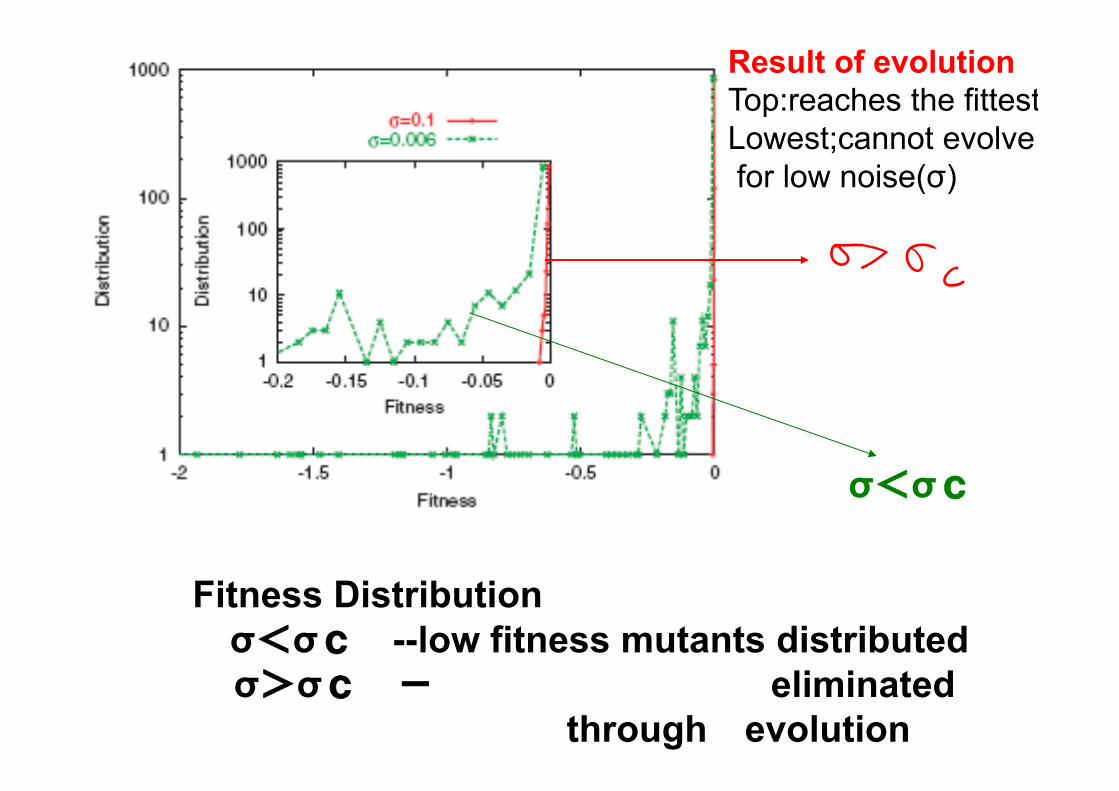
Fitness Distributionσ＜σｃ --low fitness mutants distributedσ＞σｃ － eliminated

through evolution

σ＜σｃ

Result of evolutionTop:reaches the fittestLowest;cannot evolvefor low noise(σ)

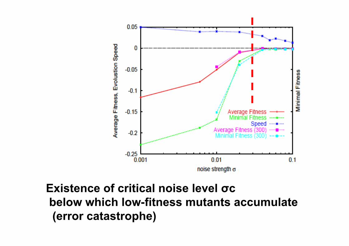
Existence of critical noise level σcbelow which low-fitness mutants accumulate(error catastrophe)

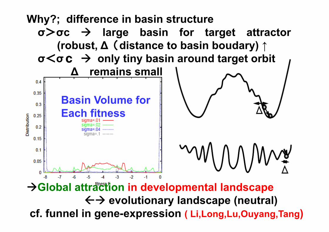
Why?; difference in basin structureσ＞σc large basin for target attractor

(robust, ∆（distance to basin boudary) ↑σ＜σｃ only tiny basin around target orbit

∆ remains small

Basin Volume forEach fitness

Global attraction in developmental landscape evolutionary landscape (neutral)

cf. funnel in gene-expression ( Li,Long,Lu,Ouyang,Tang)

why threshold?

choose paths to avoid turning pts within σ (noise)

Mutation→ touches turningpoints within range of μ

small σ －＞an orbit with small ∆can reach the target

∆

∆

∆

∆

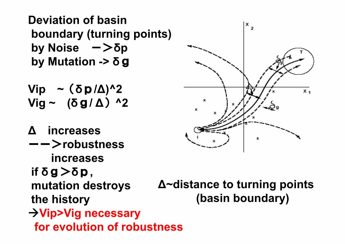
Deviation of basinboundary (turning points)by Noise －＞δpby Mutation -> δｇ

Vip ~（δｐ/∆)^2Vig ~ (δｇ/ ∆）^2

∆ increasesーー＞robustness

increasesif δｇ＞δｐ, mutation destroysthe historyVip>Vig necessaryfor evolution of robustness

∆~distance to turning points(basin boundary)

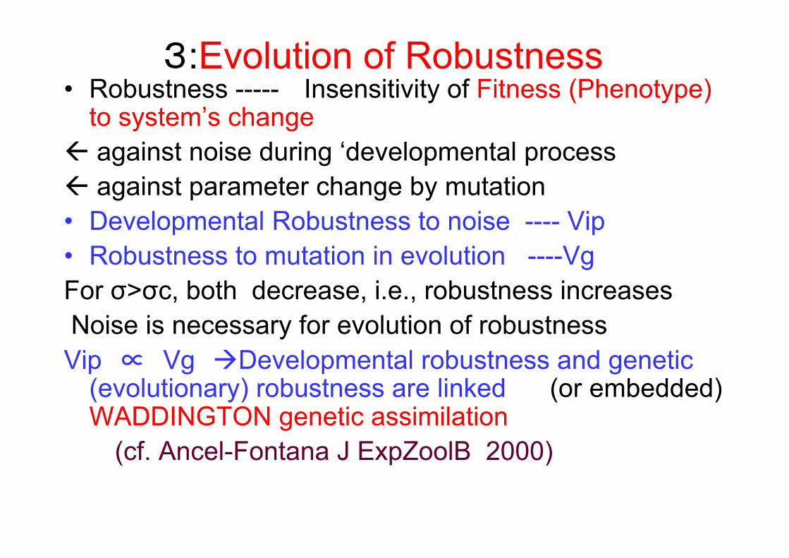
３:Evolution of Robustness• Robustness ----- Insensitivity of Fitness (Phenotype)

to system’s change against noise during ‘developmental process against parameter change by mutation• Developmental Robustness to noise ---- Vip• Robustness to mutation in evolution ----VgFor σ>σc, both decrease, i.e., robustness increasesNoise is necessary for evolution of robustnessVip ∝ Vg Developmental robustness and genetic

(evolutionary) robustness are linked (or embedded) WADDINGTON genetic assimilation

(cf. Ancel-Fontana J ExpZoolB 2000)

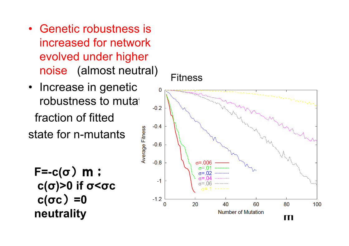
• Genetic robustness is increased for network evolved under higher noise (almost neutral)

• Increase in genetic robustness to mutation

fraction of fitted state for n-mutants

m

F=-c(σ）ｍ；c(σ)>0 if σ<σcc(σc）=0neutrality

Fitness

Ts: noise during‘developmental’ dynamicsMonte Carlo with exp(-H/Ts)

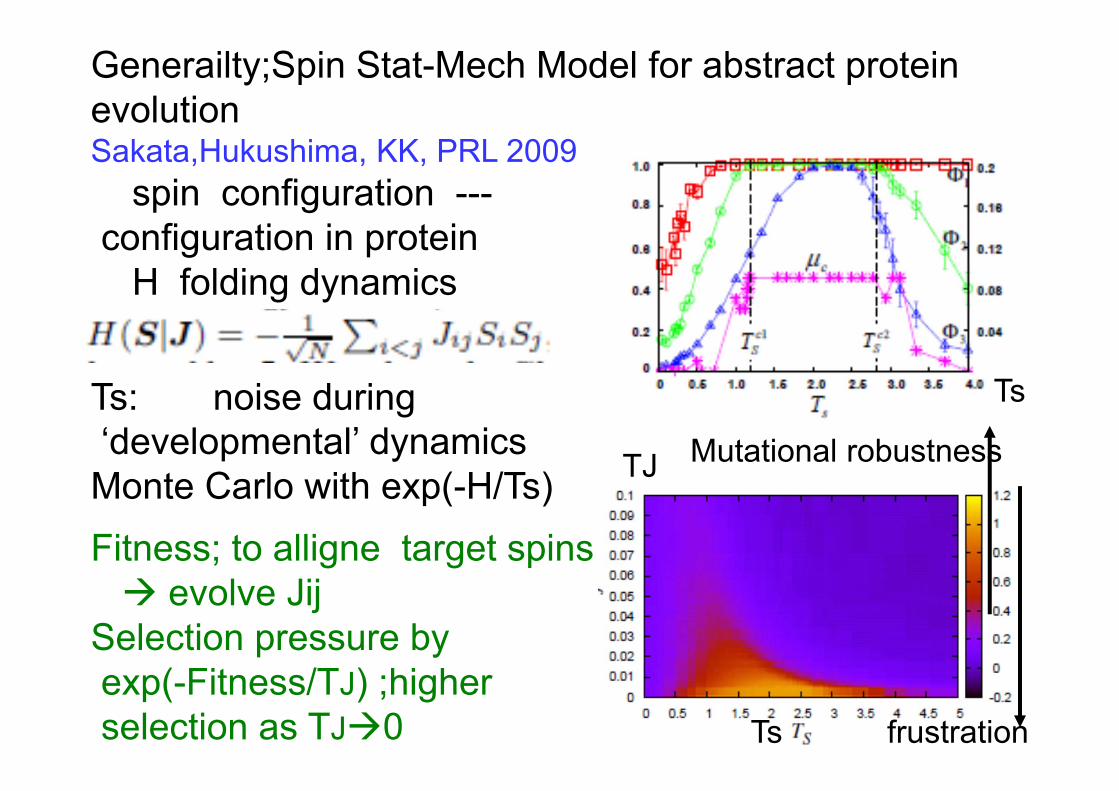
Generailty;Spin Stat-Mech Model for abstract protein evolution Sakata,Hukushima, KK, PRL 2009

spin configuration ---configuration in protein

H folding dynamics

Fitness; to alligne target spins evolve Jij

Selection pressure by exp(-Fitness/TJ) ;higherselection as TJ0

Mutational robustness

frustration

TJ

Ts

Ts

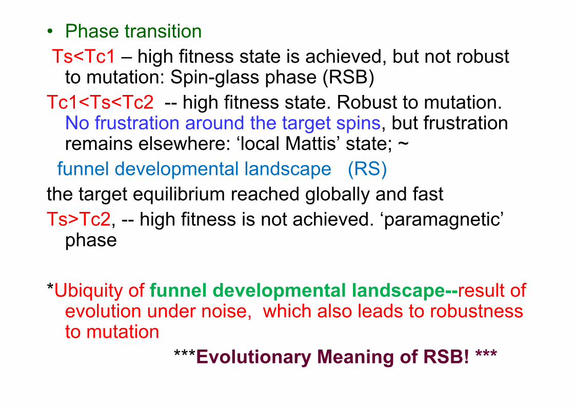
• Phase transitionTs<Tc1 – high fitness state is achieved, but not robust

to mutation: Spin-glass phase (RSB)Tc1<Ts<Tc2 -- high fitness state. Robust to mutation.

No frustration around the target spins, but frustration remains elsewhere: ‘local Mattis’ state; ~

funnel developmental landscape (RS)the target equilibrium reached globally and fastTs>Tc2, -- high fitness is not achieved. ‘paramagnetic’

phase

*Ubiquity of funnel developmental landscape--result of evolution under noise, which also leads to robustness to mutation

***Evolutionary Meaning of RSB! ***

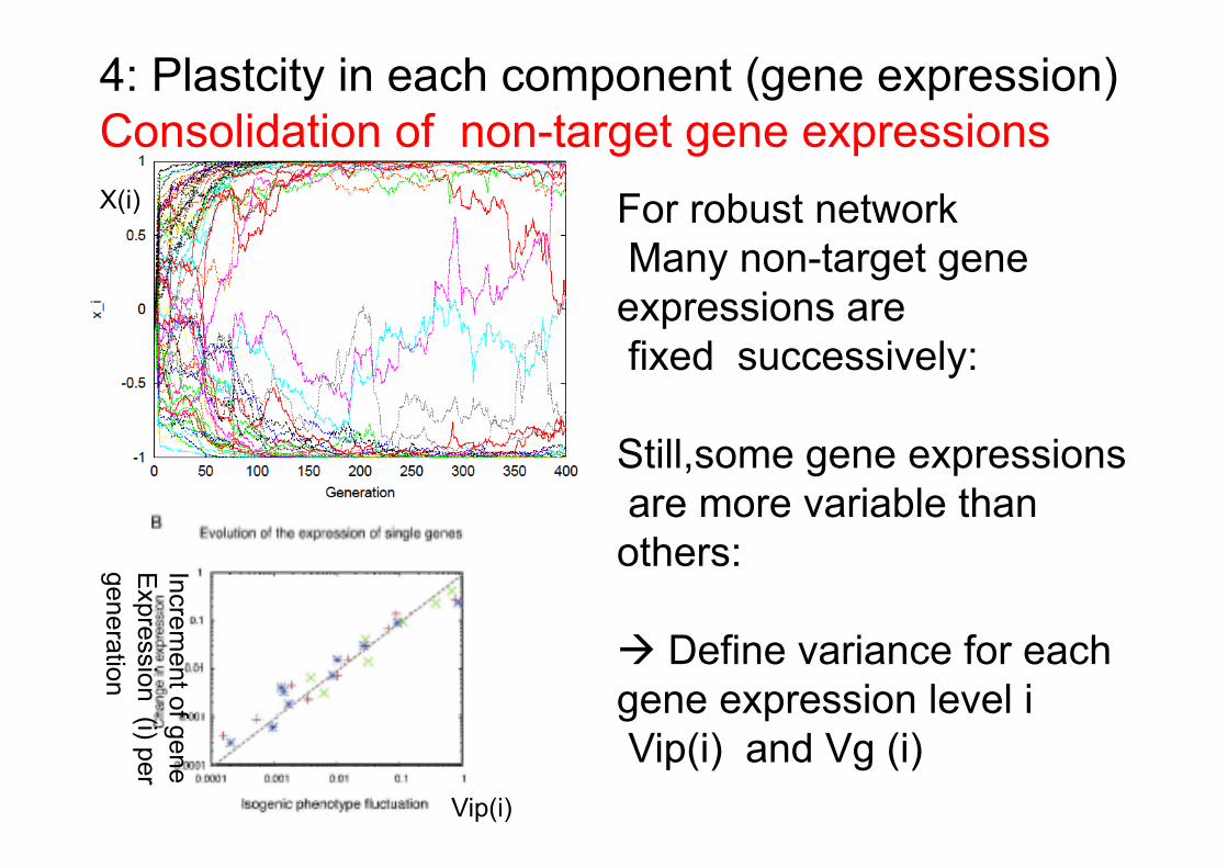
4: Plastcity in each component (gene expression) Consolidation of non-target gene expressions

For robust networkMany non-target gene expressions are fixed successively:

Still,some gene expressionsare more variable than others:

Define variance for each gene expression level iVip(i) and Vg (i)

X(i)

Vip(i)

Increment of gene

Expression (i) per

generation

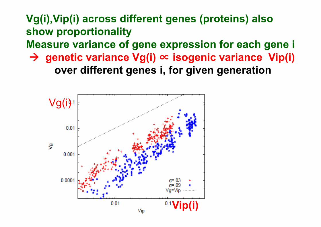
Vg(i),Vip(i) across different genes (proteins) also show proportionalityMeasure variance of gene expression for each gene i genetic variance Vg(i) ∝ isogenic variance Vip(i)

over different genes i, for given generation

Vg(i)

Vip(i)

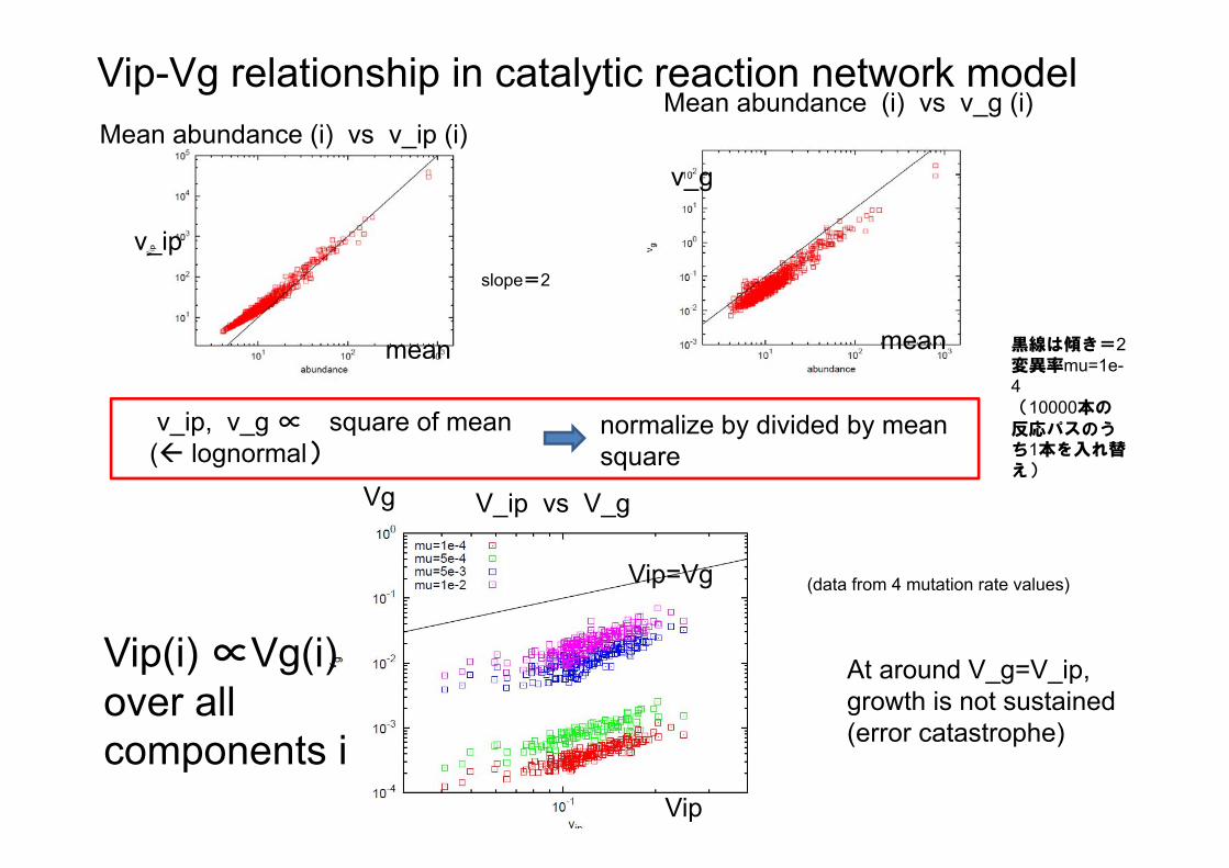
Mean abundance (i) vs v_ip (i)Mean abundance (i) vs v_g (i)

黒線は傾き＝2変異率mu=1e-4（10000本の

反応パスのうち1本を入れ替え）

slope＝2

v_ip, v_g ∝ square of mean( lognormal）

normalize by divided by mean square

V_ip vs V_g

(data from 4 mutation rate values)

At around V_g=V_ip, growth is not sustained (error catastrophe)

Vip(i) ∝Vg(i)over allcomponents i

Vip=Vg

Vip

Vg

Vip-Vg relationship in catalytic reaction network model

mean

v_ip

mean

v_g

~Vip

Experimental evidences

Mutationalvariance~ Vg

Expression Noise ~ Vip

Science 08

Courtesy of Ben Lehner

yeastFruit fly

After selectionWithout selection

Wｈｙ existence of universal proportionality relationship? Existence of ‘developmental temperature’ to support ‘fluctuation-dissipation-type relationship?

No answer yet; just only primitive argumentNote this relationship appears only after

evolution under single fitness condition;Selection under a given single fitness condition

Projection of high-dimensional gene expression dynamics to low-dimension under the fitness condition

(Projection allows for 1-dimensional collective dynamics + noise (cf Mori formalism in Stat. Mech)).

Why proportionality over genes?: Sketchy argument(i) Heuristic argument based on phenomenological distribution theory on expression of gene i

Stability For higher robustness ‘postpone’ error catastrophe. Then it occurs simultaneously common error threshold

Indep’t of (most) genes i

~ constant

NB: Vg-Vip proportionality law is a result of evolution

Most gene expressions are dominated by such ‘collective modes’ in developmental landscape that is correlated with evolutionary landscape

Recall Vg/Vip=μ/μ_max. This could be applied to any genes. In general, the mutation for the ‘error catastrophe’ can differ by genes. But assuming that genes are mutually correlated through the above low-dimensional collective dynamics, at such error threshold, the collective dynamics collapse. Then fixation of most genes (i.e., single-peaked-ness in each gene expression distribution) collapses simultaneously at the same μ. Then one may expect universal μmax, which may imply universal Vip-Vg relationship

(ii)A heuristic argument on Vip-Vg law:Self-consistent fluctuation --

Assume collective variable F and its fluctuation

• Generality of our result; (probably..) Iffitness is determined after developmental dynamics,

sufficiently ‘’complex’’ (nonlinear)(errors are often generated, fitted ones are rare)

----------------------------------------------------------------*Vip variance of phenotype over isogenic individuals*Vg variance of average phenotype over heterogenic

populationPlasticity ∝ Vip ∝ Vg ∝ evolution speed

through evolution course & over different phenotypesProperty as a result of evolution under fixed fitness cond.If more variable by developmental or environmental

noise, also variable by mutation ( qunatitative representation of genetic assimilation by Waddington)

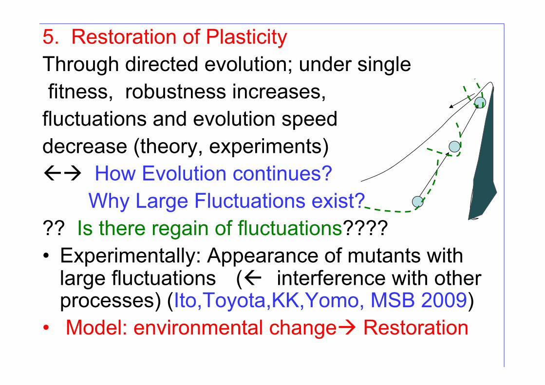
5. Restoration of PlasticityThrough directed evolution; under singlefitness, robustness increases,fluctuations and evolution speeddecrease (theory, experiments) How Evolution continues?

Why Large Fluctuations exist??? Is there regain of fluctuations????• Experimentally: Appearance of mutants with

large fluctuations ( interference with other processes) (Ito,Toyota,KK,Yomo, MSB 2009)

• Model: environmental change Restoration

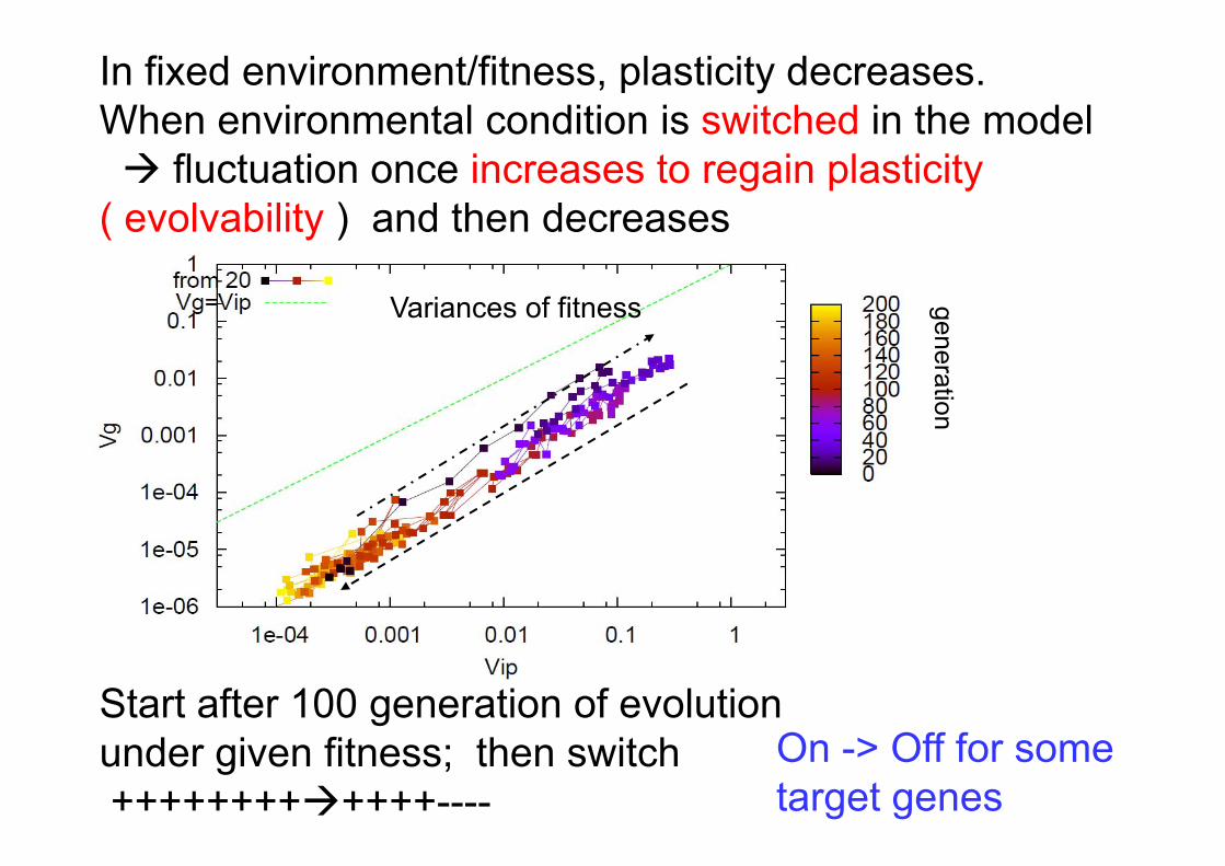
In fixed environment/fitness, plasticity decreases. When environmental condition is switched in the model fluctuation once increases to regain plasticity

( evolvability ) and then decreases

Start after 100 generation of evolution under given fitness; then switch ++++++++++++----

On -> Off for some target genes

generationVariances of fitness

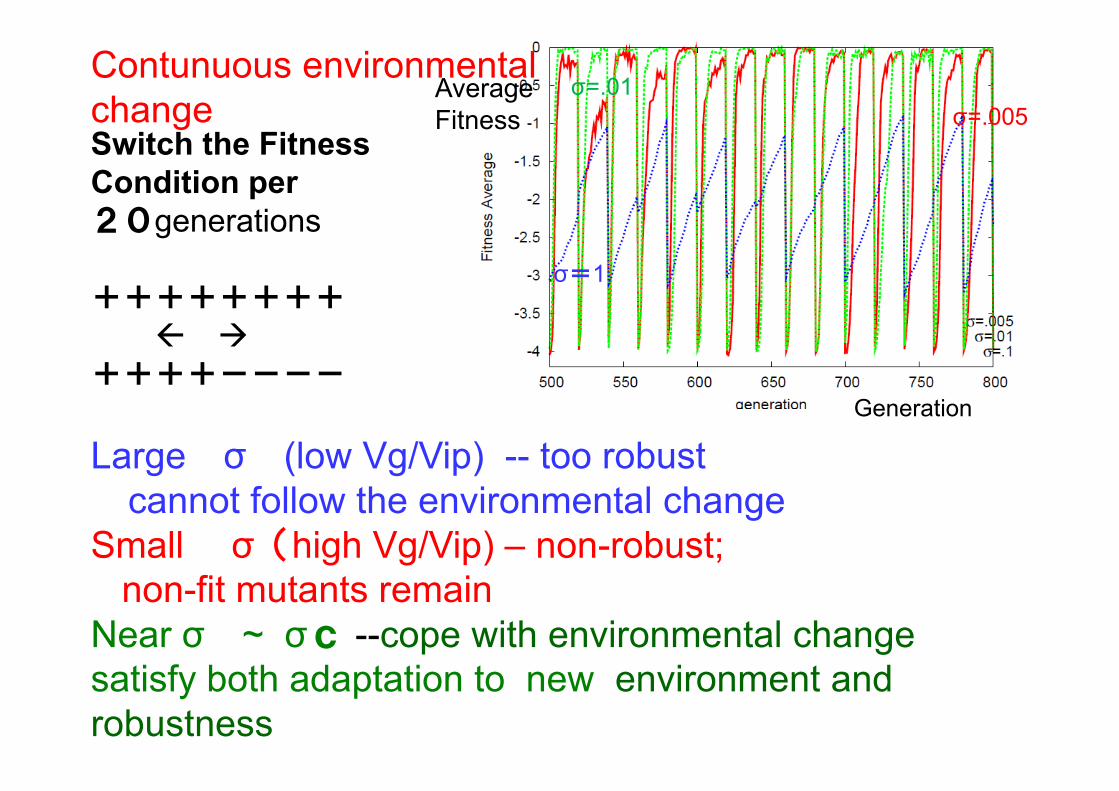
Switch the FitnessCondition per ２０generations

＋＋＋＋＋＋＋＋

＋＋＋＋－－－－

Large σ (low Vg/Vip) -- too robustcannot follow the environmental change

Small σ（high Vg/Vip) – non-robust;non-fit mutants remain

Near σ ~ σｃ --cope with environmental changesatisfy both adaptation to new environment and robustness

AverageFitness

Contunuous environmentalchange

Generation

.σ＝1

σ=.01σ=.005

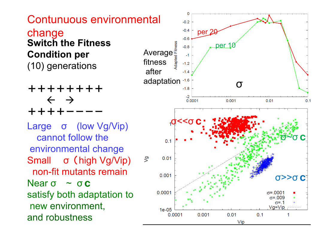
Switch the FitnessCondition per (10) generations

＋＋＋＋＋＋＋＋

＋＋＋＋－－－－

Large σ (low Vg/Vip)cannot follow the

environmental changeSmall σ（high Vg/Vip)non-fit mutants remain

Near σ ~ σｃsatisfy both adaptation to new environment, and robustness

Contunuous environmentalchange

Average fitnessafter adaptation σ

per 20

per 10

σ<<σｃσ~σｃ

σ>>σｃ

-FitnessVipVip

Vg

Vg

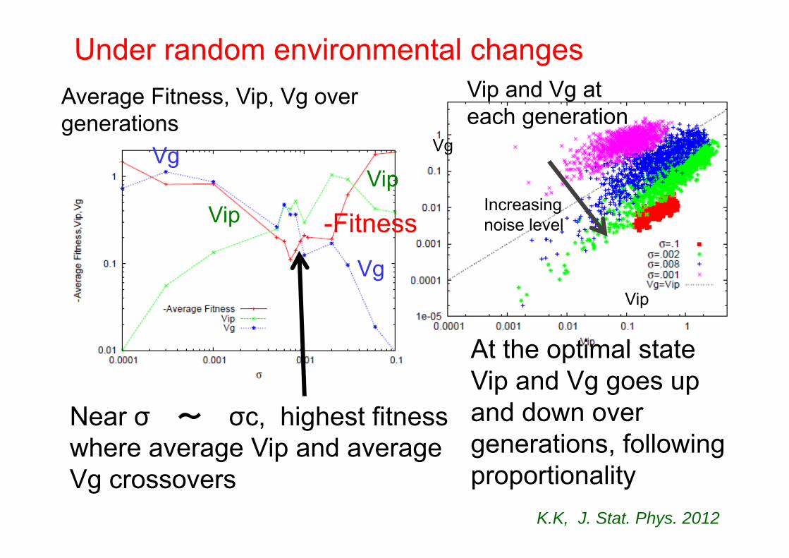
Near σ 〜 σc, highest fitnesswhere average Vip and averageVg crossovers

At the optimal stateVip and Vg goes up and down over generations, following proportionality

Average Fitness, Vip, Vg over generations

Vip and Vg at each generation

Vip

Vg

Increasing noise level

K.K, J. Stat. Phys. 2012

Under random environmental changes

-0.6 -0.4 -0.2 0.0 0.2 0.40.00

0.02

0.04

0.06

0.08

-0.6 -0.4 -0.2 0.0 0.2 0.40.00

0.02

0.04

0.06

0.08

Fig.1

B

-0.6 -0.4 -0.2 0.0 0.2 0.40.00

0.02

0.04

0.06

0.08

A

C D

GFP fluorescence (a.u.)

Forw

ard

Scat

ter (

a.u.

)

Log (GFP/FS) Log (GFP/FS) Log (GFP/FS)

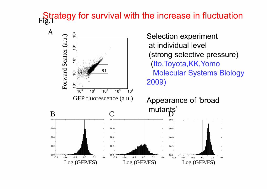
Selection experimentat individual level(strong selective pressure)(Ito,Toyota,KK,YomoMolecular Systems Biology

2009)

Appearance of ‘broadmutants’

Strategy for survival with the increase in fluctuation

-1.0 -0.5 0.00

1

2

3

4

5

Log Peak value (a.u.)

Fluctuation

Peak Folurescence value

Emergence of Broad Mutants

Not due to Plasmid number VarianceCorrelated with concentrationof mRNA (through cell growthdynamics) Use of ‘new’ degrees

of freedom

Appears frommany branches

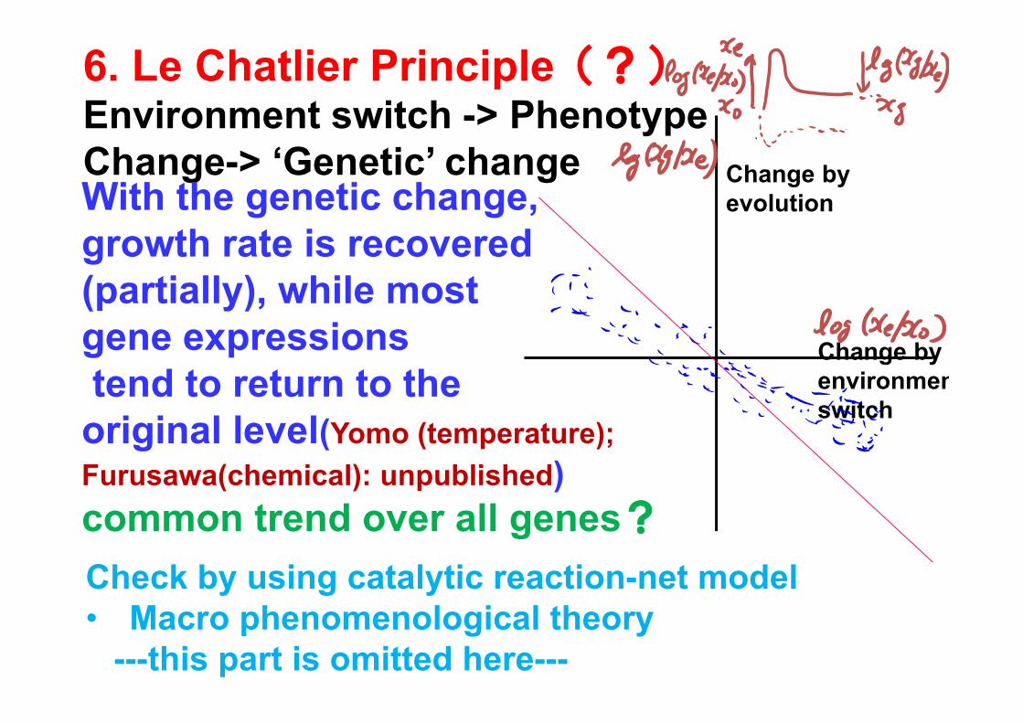
6. Le Chatlier Principle（？）Environment switch -> Phenotype Change-> ‘Genetic’ changeWith the genetic change, growth rate is recovered (partially), while most gene expressions tend to return to the original level(Yomo (temperature); Furusawa(chemical): unpublished)common trend over all genes？

Change by environmenswitch

Change by evolution

Check by using catalytic reaction-net model• Macro phenomenological theory

---this part is omitted here---

• Probably.....Existence of  

macroscopic phenomenological theory  a la thermodynamics (for universal biology)

Waiting for Carnot and Clausius of 21th century??Short History: Macro‐state theory(‘Systems Physics’)

~1860 Thermodynamics (Clausius,…)~1910 Relativity, Brownian motion (Einstein)~1960 Chaos (Lorenz,…)~2010 ????? 

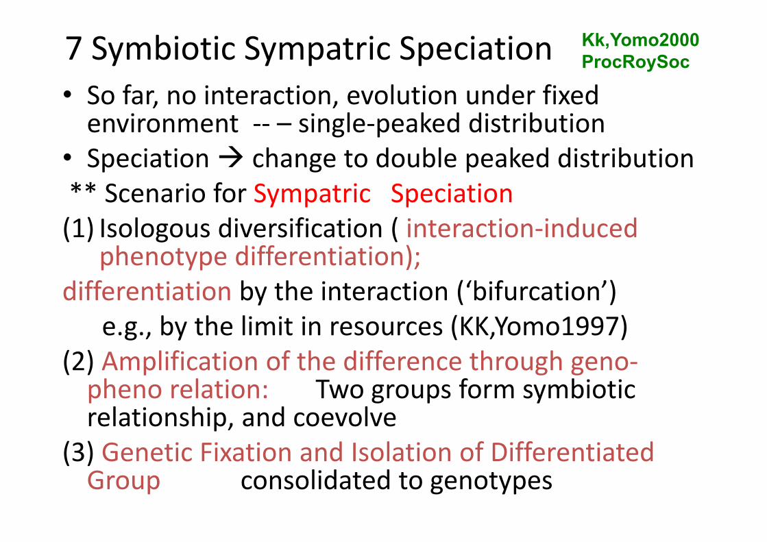
7 Symbiotic Sympatric Speciation• So far, no interaction, evolution under fixed environment  ‐‐ – single‐peaked distribution

• Speciation  change to double peaked distribution** Scenario for Sympatric Speciation(1) Isologous diversification ( interaction‐induced

phenotype differentiation); differentiation by the interaction (‘bifurcation’)

e.g., by the limit in resources (KK,Yomo1997)(2) Amplification of the difference through geno‐pheno relation:    Two groups form symbiotic relationship, and coevolve

(3) Genetic Fixation and Isolation of Differentiated Group consolidated to genotypes

Kk,Yomo2000ProcRoySoc

1 Isogenic Phenotypic Fluctuation (Plasticity) ∝Evolution2 Isogenic Phenotypic Fluctuation ∝ Genetic

Variance3 Evolution of Robustness to Noise∝to Mutation4 Plasticity of each phenotype： Vg(i)/Vip(i)〜const5 Restoration of Plasticity to increase variances6 LeChatlier Principle? Macro Phenomenology?

7 Symbiotic Sympatric Speciation8 Evolution of Morphogenesis

Evolution –shaping dynamical systems by dynamical systems

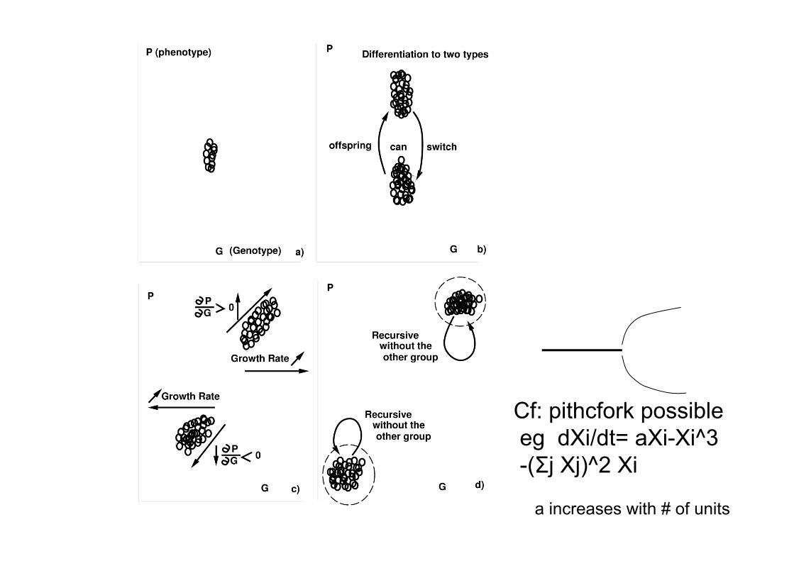
Cf: pithcfork possible eg dXi/dt= aXi-Xi^3-(Σj Xj)^2 Xi

a increases with # of units

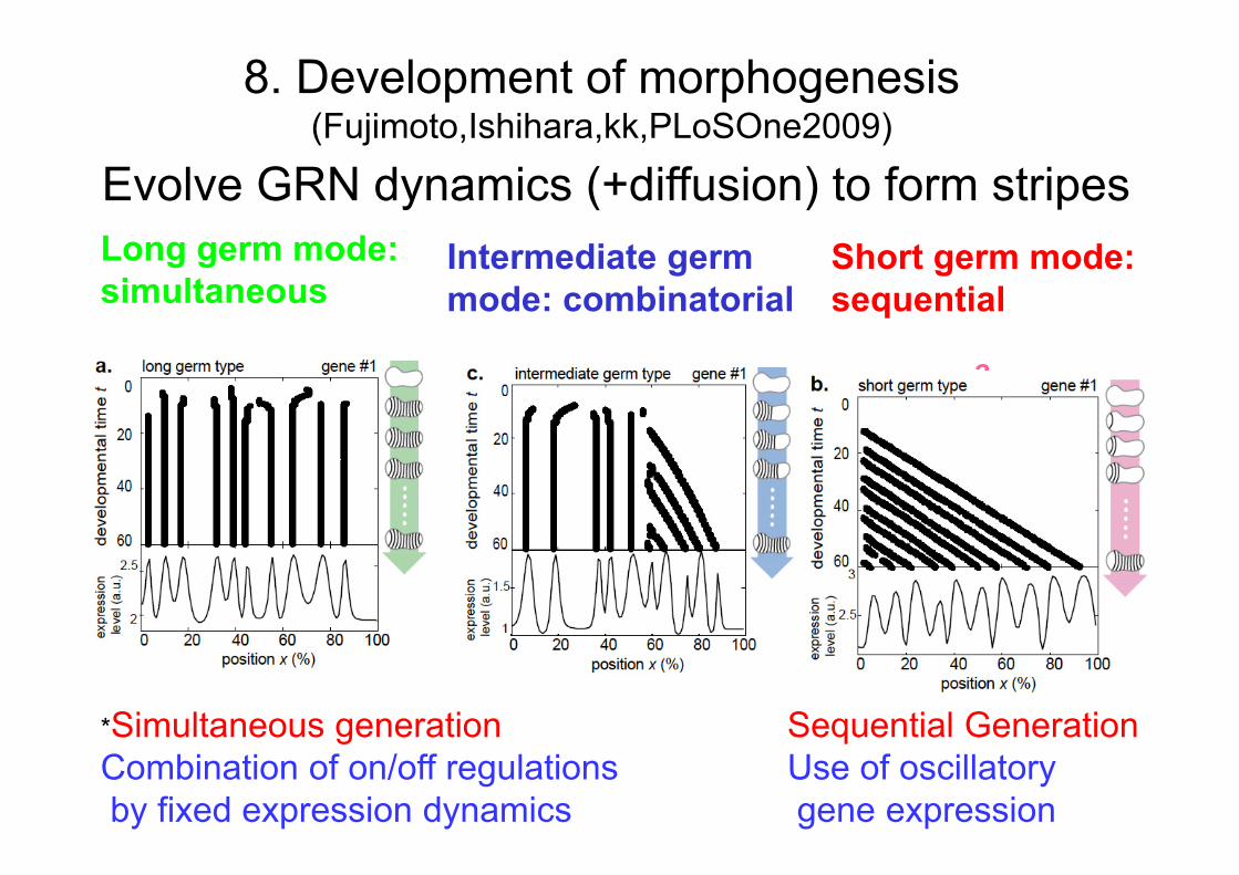
Long germ mode: simultaneous

Intermediate germ mode: combinatorial

Short germ mode: sequential

3

8. Development of morphogenesis (Fujimoto,Ishihara,kk,PLoSOne2009)

*Simultaneous generationCombination of on/off regulationsby fixed expression dynamics

Sequential GenerationUse of oscillatorygene expression

Evolve GRN dynamics (+diffusion) to form stripes

FFLsFBL +FFL

FBL

Network module

necessary

?

No need

Spatial Hierarchy

Higher

Lower

Mutation rate

Slower

Faster

Development

varietycombinatorialIntermediatevariety

simple

Knockout response

simultaneousLong

sequentialShort

Pattern formation

Segmentation mode

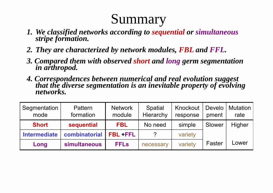
Summary1. We classified networks according to sequential or simultaneous

stripe formation. 2. They are characterized by network modules, FBL and FFL. 3. Compared them with observed short and long germ segmentation

in arthropod.4. Correspondences between numerical and real evolution suggest

that the diverse segmentation is an inevitable property of evolving networks.

CollaboratorsChikara Furusawa

Katsuhiko Satoexperiment

Tetsuya YomoYoichiro Ito

Most papers available athttp://chaos.c.u-tokyo.ac.jp

KK, PLoS One 20072012 In Evolutionary Systems BiologyKK & Furusawa, JTB 2006 + in prep

Sato etal PNAS 2003Ito et al MSB 2009Also Sakata,Hukushima,kk,PRL2009Cf. KK,Yomo, ProcRoySoc 2000,Fujimoto,Ishihara,KK,2009)