Plantar fascia segmentation and thickness estimation in ultrasound images

Boussouar, A and Meziane, F

http://dx.doi.org/10.1016/j.compmedimag.2017.02.001

Title Plantar fascia segmentation and thickness estimation in ultrasound images

Authors Boussouar, A and Meziane, F

Type Article

URL This version is available at: http://usir.salford.ac.uk/41412/

Published Date 2017

USIR is a digital collection of the research output of the University of Salford. Where copyright permits, full text material held in the repository is made freely available online and can be read, downloaded and copied for non­commercial private study or research purposes. Please check the manuscript for any further copyright restrictions.

For more information, including our policy and submission procedure, pleasecontact the Repository Team at: usir@salford.ac.uk.

Pi

Aa

b

a

ARRA

KUSPSR(FC

1

ttotlaebeoi

f

h0

Computerized Medical Imaging and Graphics 56 (2017) 60–73

Contents lists available at ScienceDirect

Computerized Medical Imaging and Graphics

j ourna l h omepa ge: www.elsev ier .com/ locate /compmedimag

lantar fascia segmentation and thickness estimation in ultrasoundmages

bdelhafid Boussouar a,∗, Farid Meziane a, Gillian Crofts b

School of Computing, Science and Engineering, University of Salford, Salford, Manchester M6 6PU, United KingdomSchool of Health Sciences, University of Salford, Salford, Manchester M5 4WT, United Kingdom

r t i c l e i n f o

rticle history:eceived 7 September 2016eceived in revised form 9 January 2017ccepted 13 February 2017

eywords:ltrasound (US)peckle noiselantar fascia (PF)egmentationadial Basic Function Neural NetworkRBF-NN)eature extractionlassification

a b s t r a c t

Ultrasound (US) imaging offers significant potential in diagnosis of plantar fascia (PF) injury and moni-toring treatment. In particular US imaging has been shown to be reliable in foot and ankle assessmentand offers a real-time effective imaging technique that is able to reliably confirm structural changes, suchas thickening, and identify changes in the internal echo structure associated with diseased or damagedtissue. Despite the advantages of US imaging, images are difficult to interpret during medical assessment.This is partly due to the size and position of the PF in relation to the adjacent tissues. It is therefore arequirement to devise a system that allows better and easier interpretation of PF ultrasound images dur-ing diagnosis. This study proposes an automatic segmentation approach which for the first time extractsultrasound data to estimate size across three sections of the PF (rearfoot, midfoot and forefoot). Thissegmentation method uses artificial neural network module (ANN) in order to classify small overlappingpatches as belonging or not-belonging to the region of interest (ROI) of the PF tissue. Features rankingand selection techniques were performed as a post-processing step for features extraction to reduce

the dimension and number of the extracted features. The trained ANN classifies the image overlappingpatches into PF and non-PF tissue, and then it is used to segment the desired PF region. The PF thick-ness was calculated using two different methods: distance transformation and area-length calculationalgorithms. This new approach is capable of accurately segmenting the PF region, differentiating it fromsurrounding tissues and estimating its thickness.

© 2017 Published by Elsevier Ltd.

. Introduction

The plantar fascia (PF) or plantar aponeurosis is an aponeurotichick, fibrous and strong connective tissue that provides stabilityo the medial longitudinal arch of the foot (Huang et al., 1993). Itriginates at the medial calcaneal tuberosity and extends towardhe digits in three different structural bands: medial, central, andateral (Chang, 2010) (Fig. 1). The central area is the largest, mostffected by disease and most susceptible to deformities (Kwongt al., 1988; Kelikian, 2012). The PF plays an important role in sta-ilizing the foot during walking and running. However, a commonly

ncountered condition is foot pain due to overuse. The assessmentf foot pain typically involves clinical examination and diagnostic

maging Park et al. (2014). The role of diagnostic imaging is to pro-

∗ Corresponding author.E-mail addresses: a.boussouar1@edu.salford.ac.uk (A. Boussouar),

.meziane@salford.ac.uk (F. Meziane), g.crofts@salford.ac.uk (G. Crofts).

ttp://dx.doi.org/10.1016/j.compmedimag.2017.02.001895-6111/© 2017 Published by Elsevier Ltd.

vide objective information which significantly then informs clinicaldecisions on treatment options. Ultrasound (US) imaging is a real-time imaging technique used in the diagnosis of the PF, which isreadily available, fast, causes no radiation exposure, portable, accu-rate, and cost-effective (Pope, 1999; Szabo, 2013). Moreover, it isconsidered highly reliable and favourable in the diagnosis of dia-betic foot with plantar fasciitis, ankle infections and damaged softtissue (Crofts et al., 2014; Angin et al., 2014; Szabo, 2013; Akfiratet al., 2003). Although US imaging offers many advantages in thediagnosis of PF conditions, it is often considered operator depen-dent when used by non-experts. In addition, the quality of imagesmay be affected by the presence of speckle noise (Ganzalez andWoods, 2002) which may diffuse the image edges, making med-ical interpretation and biometric measurements challenging, andtherefore impacting the accuracy of diagnosis.

Research has reported thickening and hypoechoic deformitiesof the PF as part of the diagnostic criteria and PF characteristicfeatures (Park et al., 2014). Increased PF thickness of >4 mm anddecreased PF echogenicity are considered symptomatic (Fabrikant

A. Boussouar et al. / Computerized Medical Imaging and Graphics 56 (2017) 60–73 61

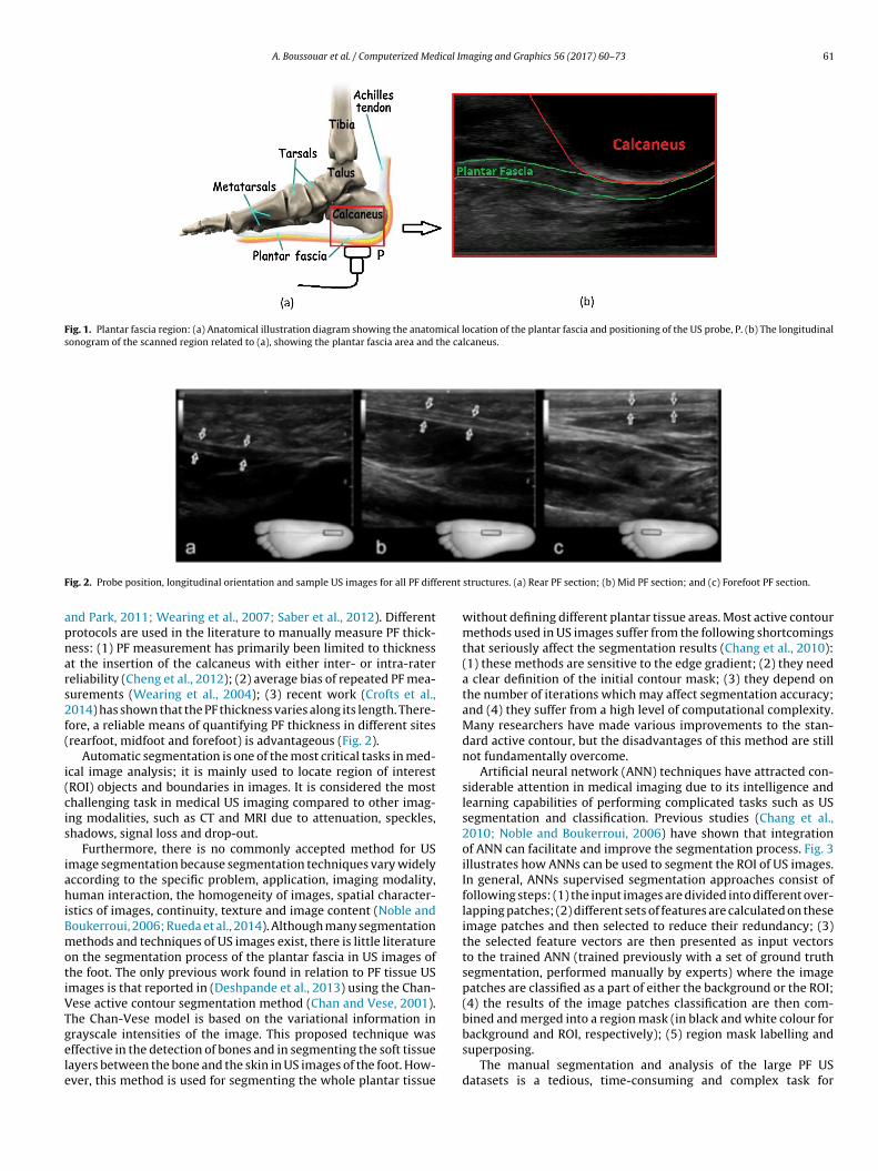
Fig. 1. Plantar fascia region: (a) Anatomical illustration diagram showing the anatomical location of the plantar fascia and positioning of the US probe, P. (b) The longitudinalsonogram of the scanned region related to (a), showing the plantar fascia area and the calcaneus.

F erent

apnars2f(

i(cis

iahiBmotiVTgele

ig. 2. Probe position, longitudinal orientation and sample US images for all PF diff

nd Park, 2011; Wearing et al., 2007; Saber et al., 2012). Differentrotocols are used in the literature to manually measure PF thick-ess: (1) PF measurement has primarily been limited to thicknesst the insertion of the calcaneus with either inter- or intra-ratereliability (Cheng et al., 2012); (2) average bias of repeated PF mea-urements (Wearing et al., 2004); (3) recent work (Crofts et al.,014) has shown that the PF thickness varies along its length. There-ore, a reliable means of quantifying PF thickness in different sitesrearfoot, midfoot and forefoot) is advantageous (Fig. 2).

Automatic segmentation is one of the most critical tasks in med-cal image analysis; it is mainly used to locate region of interestROI) objects and boundaries in images. It is considered the mosthallenging task in medical US imaging compared to other imag-ng modalities, such as CT and MRI due to attenuation, speckles,hadows, signal loss and drop-out.

Furthermore, there is no commonly accepted method for USmage segmentation because segmentation techniques vary widelyccording to the specific problem, application, imaging modality,uman interaction, the homogeneity of images, spatial character-

stics of images, continuity, texture and image content (Noble andoukerroui, 2006; Rueda et al., 2014). Although many segmentationethods and techniques of US images exist, there is little literature

n the segmentation process of the plantar fascia in US images ofhe foot. The only previous work found in relation to PF tissue USmages is that reported in (Deshpande et al., 2013) using the Chan-ese active contour segmentation method (Chan and Vese, 2001).he Chan-Vese model is based on the variational information in

rayscale intensities of the image. This proposed technique wasffective in the detection of bones and in segmenting the soft tissueayers between the bone and the skin in US images of the foot. How-ver, this method is used for segmenting the whole plantar tissue

structures. (a) Rear PF section; (b) Mid PF section; and (c) Forefoot PF section.

without defining different plantar tissue areas. Most active contourmethods used in US images suffer from the following shortcomingsthat seriously affect the segmentation results (Chang et al., 2010):(1) these methods are sensitive to the edge gradient; (2) they needa clear definition of the initial contour mask; (3) they depend onthe number of iterations which may affect segmentation accuracy;and (4) they suffer from a high level of computational complexity.Many researchers have made various improvements to the stan-dard active contour, but the disadvantages of this method are stillnot fundamentally overcome.

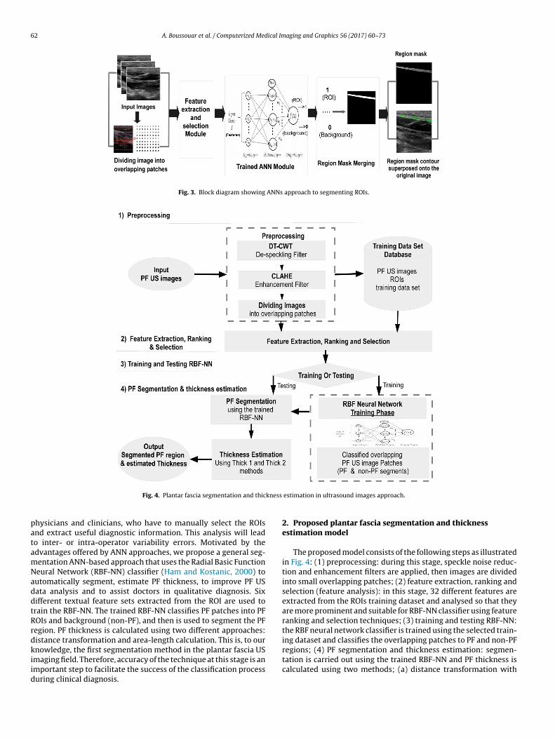
Artificial neural network (ANN) techniques have attracted con-siderable attention in medical imaging due to its intelligence andlearning capabilities of performing complicated tasks such as USsegmentation and classification. Previous studies (Chang et al.,2010; Noble and Boukerroui, 2006) have shown that integrationof ANN can facilitate and improve the segmentation process. Fig. 3illustrates how ANNs can be used to segment the ROI of US images.In general, ANNs supervised segmentation approaches consist offollowing steps: (1) the input images are divided into different over-lapping patches; (2) different sets of features are calculated on theseimage patches and then selected to reduce their redundancy; (3)the selected feature vectors are then presented as input vectorsto the trained ANN (trained previously with a set of ground truthsegmentation, performed manually by experts) where the imagepatches are classified as a part of either the background or the ROI;(4) the results of the image patches classification are then com-bined and merged into a region mask (in black and white colour for

background and ROI, respectively); (5) region mask labelling andsuperposing.

The manual segmentation and analysis of the large PF USdatasets is a tedious, time-consuming and complex task for

62 A. Boussouar et al. / Computerized Medical Imaging and Graphics 56 (2017) 60–73

Fig. 3. Block diagram showing ANNs approach to segmenting ROIs.

kness

patamNaddtRrdkiid

Fig. 4. Plantar fascia segmentation and thic

hysicians and clinicians, who have to manually select the ROIsnd extract useful diagnostic information. This analysis will leado inter- or intra-operator variability errors. Motivated by thedvantages offered by ANN approaches, we propose a general seg-entation ANN-based approach that uses the Radial Basic Functioneural Network (RBF-NN) classifier (Ham and Kostanic, 2000) toutomatically segment, estimate PF thickness, to improve PF USata analysis and to assist doctors in qualitative diagnosis. Sixifferent textual feature sets extracted from the ROI are used torain the RBF-NN. The trained RBF-NN classifies PF patches into PFOIs and background (non-PF), and then is used to segment the PFegion. PF thickness is calculated using two different approaches:istance transformation and area-length calculation. This is, to ournowledge, the first segmentation method in the plantar fascia US

maging field. Therefore, accuracy of the technique at this stage is anmportant step to facilitate the success of the classification processuring clinical diagnosis.

estimation in ultrasound images approach.

2. Proposed plantar fascia segmentation and thicknessestimation model

The proposed model consists of the following steps as illustratedin Fig. 4: (1) preprocessing: during this stage, speckle noise reduc-tion and enhancement filters are applied, then images are dividedinto small overlapping patches; (2) feature extraction, ranking andselection (feature analysis): in this stage, 32 different features areextracted from the ROIs training dataset and analysed so that theyare more prominent and suitable for RBF-NN classifier using featureranking and selection techniques; (3) training and testing RBF-NN:the RBF neural network classifier is trained using the selected train-ing dataset and classifies the overlapping patches to PF and non-PFregions; (4) PF segmentation and thickness estimation: segmen-

tation is carried out using the trained RBF-NN and PF thickness iscalculated using two methods; (a) distance transformation with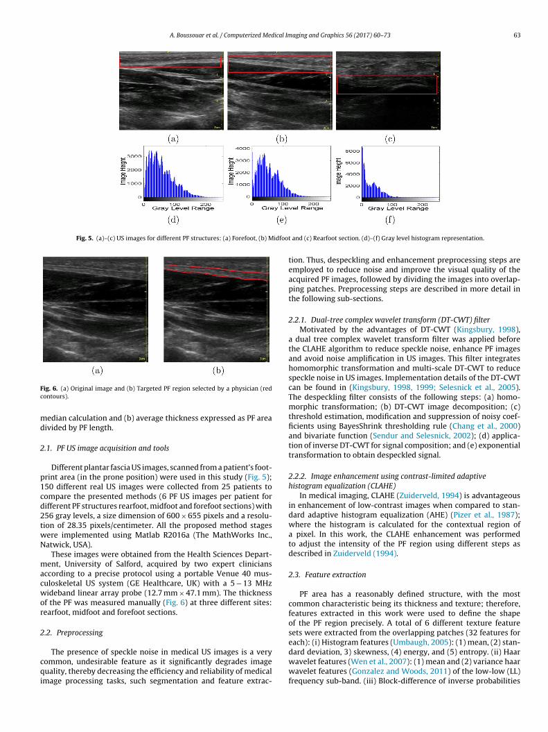

A. Boussouar et al. / Computerized Medical Imaging and Graphics 56 (2017) 60–73 63

Fig. 5. (a)–(c) US images for different PF structures: (a) Forefoot, (b) Midfoot

Fc

md

2

p1cd2twN

macwor

2

cqi

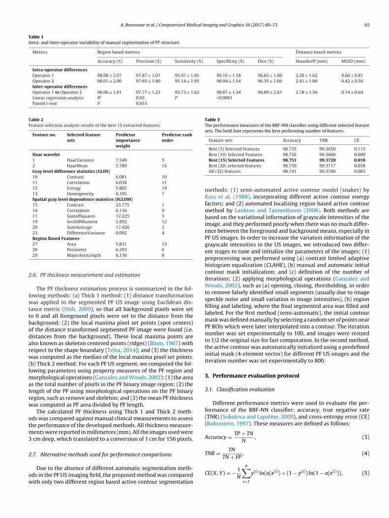
ig. 6. (a) Original image and (b) Targeted PF region selected by a physician (redontours).

edian calculation and (b) average thickness expressed as PF areaivided by PF length.

.1. PF US image acquisition and tools

Different plantar fascia US images, scanned from a patient’s foot-rint area (in the prone position) were used in this study (Fig. 5);50 different real US images were collected from 25 patients toompare the presented methods (6 PF US images per patient forifferent PF structures rearfoot, midfoot and forefoot sections) with56 gray levels, a size dimension of 600 × 655 pixels and a resolu-ion of 28.35 pixels/centimeter. All the proposed method stagesere implemented using Matlab R2016a (The MathWorks Inc.,atwick, USA).

These images were obtained from the Health Sciences Depart-ent, University of Salford, acquired by two expert clinicians

ccording to a precise protocol using a portable Venue 40 mus-uloskeletal US system (GE Healthcare, UK) with a 5 − 13 MHzideband linear array probe (12.7 mm × 47.1 mm). The thickness

f the PF was measured manually (Fig. 6) at three different sites:earfoot, midfoot and forefoot sections.

.2. Preprocessing

The presence of speckle noise in medical US images is a veryommon, undesirable feature as it significantly degrades imageuality, thereby decreasing the efficiency and reliability of medical

mage processing tasks, such segmentation and feature extrac-

and (c) Rearfoot section. (d)–(f) Gray level histogram representation.

tion. Thus, despeckling and enhancement preprocessing steps areemployed to reduce noise and improve the visual quality of theacquired PF images, followed by dividing the images into overlap-ping patches. Preprocessing steps are described in more detail inthe following sub-sections.

2.2.1. Dual-tree complex wavelet transform (DT-CWT) filterMotivated by the advantages of DT-CWT (Kingsbury, 1998),

a dual tree complex wavelet transform filter was applied beforethe CLAHE algorithm to reduce speckle noise, enhance PF imagesand avoid noise amplification in US images. This filter integrateshomomorphic transformation and multi-scale DT-CWT to reducespeckle noise in US images. Implementation details of the DT-CWTcan be found in (Kingsbury, 1998, 1999; Selesnick et al., 2005).The despeckling filter consists of the following steps: (a) homo-morphic transformation; (b) DT-CWT image decomposition; (c)threshold estimation, modification and suppression of noisy coef-ficients using BayesShrink thresholding rule (Chang et al., 2000)and bivariate function (Sendur and Selesnick, 2002); (d) applica-tion of inverse DT-CWT for signal composition; and (e) exponentialtransformation to obtain despeckled signal.

2.2.2. Image enhancement using contrast-limited adaptivehistogram equalization (CLAHE)

In medical imaging, CLAHE (Zuiderveld, 1994) is advantageousin enhancement of low-contrast images when compared to stan-dard adaptive histogram equalization (AHE) (Pizer et al., 1987);where the histogram is calculated for the contextual region ofa pixel. In this work, the CLAHE enhancement was performedto adjust the intensity of the PF region using different steps asdescribed in Zuiderveld (1994).

2.3. Feature extraction

PF area has a reasonably defined structure, with the mostcommon characteristic being its thickness and texture; therefore,features extracted in this work were used to define the shapeof the PF region precisely. A total of 6 different texture featuresets were extracted from the overlapping patches (32 features foreach): (i) Histogram features (Umbaugh, 2005): (1) mean, (2) stan-

dard deviation, 3) skewness, (4) energy, and (5) entropy. (ii) Haarwavelet features (Wen et al., 2007): (1) mean and (2) variance haarwavelet features (Gonzalez and Woods, 2011) of the low-low (LL)frequency sub-band. (iii) Block-difference of inverse probabilities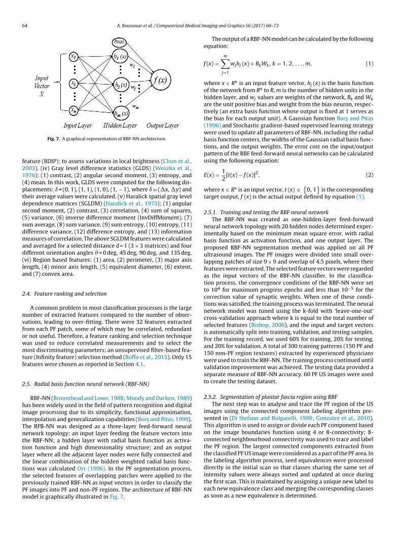

64 A. Boussouar et al. / Computerized Medical Im

f21(ptds(sdmad(la

2

nvfowmtf

2

hiiTnttltttpPm

intensity values were always sorted and updated at once during

Fig. 7. A graphical representation of RBF-NN architecture.

eature (BDIP): to assess variations in local brightness (Chun et al.,003). (iv) Gray level difference statistics (GLDS) (Weszka et al.,976): (1) contrast, (2) angular second moment, (3) entropy, and4) mean. In this work, GLDS were computed for the following dis-lacements: ı = (0, 1), (1, 1), (1, 0), (1, − 1), where ı ≡ (�x, �y) andheir average values were calculated. (v) Haralick spatial gray levelependence matrices (SGLDM) (Haralick et al., 1973): (1) angularecond moment, (2) contrast, (3) correlation, (4) sum of squares,5) variance, (6) inverse difference moment (InvDiffMoment), (7)um average, (8) sum variance, (9) sum entropy, (10) entropy, (11)ifference variance, (12) difference entropy, and (13) informationeasures of correlation. The above SGLDM features were calculated

nd averaged for a selected distance d = 1 (3 × 3 matrices) and fourifferent orientation angles � = 0 deg, 45 deg, 90 deg, and 135 deg.vi) Region based features: (1) area, (2) perimeter, (3) major axisength, (4) minor axis length, (5) equivalent diameter, (6) extent,nd (7) convex area.

.4. Feature ranking and selection

A common problem in most classification processes is the largeumber of extracted features compared to the number of obser-ations, leading to over-fitting. There were 32 features extractedrom each PF patch, some of which may be correlated, redundantr not useful. Therefore, a feature ranking and selection techniqueas used to reduce correlated measurements and to select theost discriminating parameters; an unsupervised filter-based fea-

ure (Infinity feature) selection method (Roffo et al., 2015). Only 15eatures were chosen as reported in Section 4.1.

.5. Radial basis function neural network (RBF-NN)

RBF-NN (Broomhead and Lowe, 1988; Moody and Darken, 1989)as been widely used in the field of pattern recognition and digital

mage processing due to its simplicity, functional approximation,nterpolation and generalization capabilities (Bors and Pitas, 1999).he RFB-NN was designed as a three-layer feed-forward neuraletwork topology: an input layer feeding the feature vectors intohe RBF-NN; a hidden layer with radial basis function as activa-ion function and high dimensionality structure; and an outputayer where all the adjacent layer nodes were fully connected andhe linear combination of the hidden weighted radial basis func-ions was calculated Orr (1996). In the PF segmentation process,he selected features of overlapping patches were applied to the

reviously trained RBF-NN as input vectors in order to classify theF images into PF and non-PF regions. The architecture of RBF-NNodel is graphically illustrated in Fig. 7.

aging and Graphics 56 (2017) 60–73

The output of a RBF-NN model can be calculated by the followingequation:

f (x) =m∑

j=1

wjhj (x) + BkWk, k = 1, 2, . . ., m, (1)

where x ∈ Rn is an input feature vector, hj (x) is the basis functionof the network from Rn to R, m is the number of hidden units in thehidden layer, and wj values are weights of the network, Bk and Wkare the unit positive bias and weight from the bias neuron, respec-tively (an extra basis function whose output is fixed at 1 serves asthe bias for each output unit). A Gaussian function Bors and Pitas(1996) and Stochastic gradient-based supervised learning strategywere used to update all parameters of RBF-NN, including the radialbasis function centers, the widths of the Gaussian radial basis func-tions, and the output weights. The error cost on the input/outputpattern of the RBF feed-forward neural networks can be calculatedusing the following equation:

E(x) = 12

[t(x) − f (x)]2, (2)

where x ∈ Rn is an input vector, t (x) ∈{

0, 1}

is the correspondingtarget output, f (x) is the actual output defined by equation (1).

2.5.1. Training and testing the RBF neural networkThe RBF-NN was created as one-hidden-layer feed-forward

neural network topology with 20 hidden nodes determined exper-imentally based on the minimum mean square error, with radialbasis function as activation function, and one output layer. Theproposed RBF-NN segmentation method was applied on all PFultrasound images. The PF images were divided into small over-lapping patches of size 9 × 9 and overlap of 4.5 pixels, where theirfeatures were extracted. The selected feature vectors were regardedas the input vectors of the RBF-NN classifier. In the classifica-tion process, the convergence conditions of the RBF-NN were setto 104 for maximum progress epochs and less than 10−5 for thecorrection value of synaptic weights. When one of these condi-tions was satisfied, the training process was terminated. The neuralnetwork model was tuned using the k-fold with ‘leave-one-out’cross-validation approach where k is equal to the total number ofselected features (Bishop, 2006), and the input and target vectorsis automatically split into training, validation, and testing samples.For the training record, we used 60% for training, 20% for testing,and 20% for validation. A total of 300 training patterns (150 PF and150 non-PF region textures) extracted by experienced physicianswere used to train the RBF-NN. The training process continued untilvalidation improvement was achieved. The testing data provided aseparate measure of RBF-NN accuracy. 60 PF US images were usedto create the testing dataset.

2.5.2. Segmentation of plantar fascia region using RBFThe next step was to analyse and trace the PF region of the US

images using the connected component labeling algorithm pre-sented in (Di Stefano and Bulgarelli, 1999; Gonzalez et al., 2010).This algorithm is used to assign or divide each PF component basedon the image boundaries function using 4 or 8-connectivity; 8-connected neighbourhood connectivity was used to trace and labelthe PF region. The largest connected components extracted fromthe classified PF US image were considered as a part of the PF area. Inthe labeling algorithm process, seed equivalences were processeddirectly in the initial scan so that classes sharing the same set of

the first scan. This is maintained by assigning a unique new label toeach new equivalence class and merging the corresponding classesas soon as a new equivalence is determined.

A. Boussouar et al. / Computerized Medical Imaging and Graphics 56 (2017) 60–73 65

Table 1Intra- and inter-operator variability of manual segmentation of PF structure.

Metrics Region based metrics Distance based metrics

Accuracy (%) Precision (%) Sensitivity (%) Specificity (%) Dice (%) Hausdorff (mm) MSSD (mm)

Intra-operator differencesOperator 1 98.08 ± 2.07 97.87 ± 1.07 95.97 ± 1.45 99.10 ± 1.18 96.65 ± 1.60 2.26 ± 1.62 0.66 ± 0.81Operator 2 98.01 ± 2.00 97.65 ± 1.80 95.14 ± 1.95 98.94 ± 1.54 96.35 ± 1.69 2.41 ± 1.80 0.42 ± 0.56Inter-operator differencesOperator 1 vs Operator 2 98.06 ± 1.81 97.77 ± 1.25 95.73 ± 1.62 98.87 ± 1.34 96.89 ± 2.61 2.78 ± 1.56 0.74 ± 0.64Linear regression analysis R2 0.92 P <0.0001Paired t-test P 0.853

Table 2Feature selection analysis results of the best 15 extracted features.

Feature no. Selected featuresets

Predictorimportanceweight

Predictor rankorder

Haar wavelet1 HaarVariance 7.549 52 HaarMean 5.789 15Gray level difference statistics (GLDS)10 Contrast 6.081 1011 Correlation 6.038 1112 Energy 5.802 1413 Homogeneity 6.195 7Spatial gray level dependence matrices (SGLDM)15 Contrast 23.775 116 Correlation 6.116 917 SumofSquares 12.225 319 InvDiffMoment 5.892 1220 SumAverage 17.426 223 DifferenceVariance 9.092 4Region Based Features27 Area 5.831 13

2

lwttbodarw(lmalrw

otm3

2

ow

Table 3The performance measures of the RBF-NN classifier using different selected featuresets. The bold font represents the best performing number of features.

Feature sets Accuracy TNR CE

Best (5) Selected Features 98.735 99.3650 0.115Best (10) Selected Features 98.736 99.3660 0.090Best (15) Selected Features 98.751 99.3720 0.018

28 Perimeter 6.293 629 MajorAxisLength 6.136 8

.6. PF thickness measurement and estimation

The PF thickness estimation process is summarized in the fol-owing methods: (a) Thick 1 method: (1) distance transformation

as applied to the segmented PF US image using Euclidean dis-ance metric (Shih, 2009), so that all background pixels were seto 0 and all foreground pixels were set to the distance from theackground; (2) the local maxima pixel set points (spot centers)f the distance transformed segmented PF image were found (i.e.istances from the background). These local maxima points arelso known as skeleton centered points (ridges) (Blum, 1967) withespect to the shape boundary (Telea, 2014); and (3) the thicknessas computed as the median of the local maxima pixel set points.

b) Thick 2 method: For each PF US segment, we computed the fol-owing parameters using property measures of the PF region and

orphological operations (Ganzalez and Woods, 2002): (1) the areas the total number of pixels in the PF binary image region; (2) theength of the PF using morphological operations on the PF binaryegion, such as remove and skeleton; and (3) the mean PF thicknessas computed as PF area divided by PF length.

The calculated PF thickness using Thick 1 and Thick 2 meth-ds was compared against manual clinical measurements to assesshe performance of the developed methods. All thickness measure-

ents were reported in millimetres (mm). All the images used were cm deep, which translated to a conversion of 1 cm for 156 pixels.

.7. Alternative methods used for performance comparisons

Due to the absence of different automatic segmentation meth-ds in the PF US imaging field, the proposed method was comparedith only two different region based active contour segmentation

Best (20) selected features 98.750 99.3717 0.058All (32) features 98.741 99.3700 0.083

methods: (1) semi-automated active contour model (snakes) byKass et al. (1988), incorporating different active contour energyfactors; and (2) automated localizing region based active contourmethod by Lankton and Tannenbaum (2008). Both methods arebased on the variational information of grayscale intensities of theimage, and they performed poorly when there was no much differ-ence between the foreground and background means, especially inPF US images. In order to increase the variation information of thegrayscale intensities in the US images, we introduced two differ-ent stages to tune and initialize the parameters of the images: (1)preprocessing was performed using (a) contrast limited adaptivehistogram equalization (CLAHE), (b) manual and automatic initialcontour mask initialization; and (c) definition of the number ofiterations; (2) applying morphological operations (Ganzalez andWoods, 2002), such as (a) opening, closing, thresholding, in orderto remove falsely identified small segments (usually due to imagespeckle noise and small variation in image intensities), (b) regionfilling and labeling, where the final segmented area was filled andlabeled. For the first method (semi-automatic), the initial contourmask was defined manually by selecting a random set of points nearPF ROIs which were later interpolated into a contour. The iterationnumber was set experimentally to 100, and images were resizedto 1/2 the original size for fast computation. In the second method,the active contour was automatically initialized using a predefinedinitial mask (4-element vector) for different PF US images and theiteration number was set experimentally to 800.

3. Performance evaluation protocol

3.1. Classification evaluation

Different performance metrics were used to evaluate the per-formance of the RBF-NN classifier: accuracy, true negative rate(TNR) (Sokolova and Lapalme, 2009), and cross-entropy error (CE)(Rubinstein, 1997). These measures are defined as follows:

Accuracy = TP + TN

N, (3)

TNR = TN

TN + FP, (4)

CE(X, Y) = − 1N

n∑

i=1

y(i) ln(a(x(i)) + (1 − y(i)) ln(1 − a(x(i))), (5)

66 A. Boussouar et al. / Computerized Medical Imaging and Graphics 56 (2017) 60–73

Forefoot:Ex pe rt1

Forefoot:Ex pe rt2

Midfoot:Ex pe rt1

Midfoot:Ex pe rt2

Re ar foot:Ex pe rt1

Re ar foot:Ex pe rt2

0

1

2

3

4

PFthickness(m

m)

E x p e r t 2E x p e r t 1

(a)

0 1 2 3 4

0

1

2

3

4

P F th ic k n e s s m e a su re d b y E xp e r t 1 (m m )

PFthicknessmeasuredbyExpert2(m

m)

R2= 0 .9 2

P < 0 .0 0 0 1

(b)

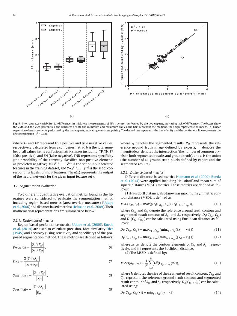
Fig. 8. Inter-operator variability: (a) differences in thickness measurements of PF structures performed by the two experts, indicating lack of differences. The boxes showt um vr iring.l

wrb((afro

3

eiem

3

e(p

P

D

S

S

he 25th and the 75th percentiles, the whiskers denote the minimum and maximegression of measurements performed by the two experts, indicating consistent paine of regression (R2 = 0.92).

here TP and TN represent true positive and true negative values,espectively, calculated from a confusion matrix, N is the total num-er of all values in the confusion matrix classes including: TP, TN, FPfalse positive), and FN (false negative). TNR represents specificitythe probability of the correctly classified non-positive elementss predicted negative). X = x(1), . . ., x(n) is the set of input selectedeatures in the training dataset, and Y = y(1), . . ., y(n) is the set of cor-esponding labels for input features. The a(x) represents the outputf the neural network for the given input feature set x.

.2. Segmentation evaluation

Two different quantitative evaluation metrics found in the lit-rature were considered to evaluate the segmentation methodncluding region-based metrics (area overlap measures) (Udupat al., 2006) and distance based metrics (Heimann et al., 2009). Theirathematical representations are summarized below.

.2.1. Region based metricsRegion based performance metrics Udupa et al. (2006), Rueda

t al. (2014) are used to calculate precision, Dice similarity Dice1945) and accuracy (using sensitivity and specificity) of the pro-osed segmentation method. These metrics are defined as follows:

recision =∣∣Sr ∩ Rgt

∣∣∣∣Sr ∪ Rgt

∣∣ , (6)

ice =2∣∣Sr ∩ Rgt

∣∣∣∣Sr + Rgt

∣∣ , (7)

ensitivity =∣∣Sr ∩ Rgt

∣∣∣∣R

∣∣ , (8)

gt

pecificity =∣∣Sr ∪ Rgt

∣∣∣∣Rgt

∣∣ , (9)

alues, the bars represent the medians, the + sign represents the means. (b) Linear The dashed line represents the line of unity and the continuous line represents the

where Sr denotes the segmented results, Rgt represents the ref-erence ground truth image defined by experts, |.| denotes themagnitude, ∩ denotes the intersection (the number of common pix-els in both segmented results and ground truth), and ∪ is the union(the number of all ground truth pixels defined by expert and thesegmented results).

3.2.2. Distance based metricsDifferent distance-based metrics Heimann et al. (2009), Rueda

et al. (2014) were applied including Hausdorff and mean sum ofsquare distance (MSSD) metrics. These metrics are defined as fol-lows:

(1) Hausdorff distance, also known as maximum symmetric con-tour distance (MSD), is defined as:

MSD(Rgt, Sr) = max((D1(CRgt , CSr ), D1(CSr , CRgt )), (10)

where CRgt and CSr denote the reference ground truth contour andsegmented result contour of Rgt and Sr, respectively. D1(CRgt , CSr )and D1(CSr , CRgt ) can be calculated using Euclidean distance as fol-lows:

D1(CRgt , CSr ) = maxx1 ∈ CRgt(minx2 ∈ CSr

(‖x1 − x2‖)) (11)

D1(CSr , CRgt ) = maxx2 ∈ CSr(minx1 ∈ CRgt

(‖x2 − x1‖)) (12)

where x1, x2 denote the contour elements of CSr and Rgt, respec-tively, and ‖.‖ represents the Euclidean distance.

(2) The MSSD is defined by:

MSSD(Rgt, Sr) = 1N

N∑

n=1

D22(CRgt , CSr (xn)), (13)

where N denotes the size of the segmented result contour, CRgt andCSr represent the reference ground truth contour and segmented

result contour of Rgt and Sr, respectively. D2(CRgt , CSr ) can be calcu-lated using:

D2(CRgt , CSr (x)) = miny ∈ Rgt (‖y − x‖) (14)

A. Boussouar et al. / Computerized Medical Imaging and Graphics 56 (2017) 60–73 67

Fig. 9. Preprocessing results: (a)–(c) Original US images for different PF structures (Forefoot, Mid and Rear section). (d)–(f) Speckle reduction results using DT-CWT filter( result

wa

3

ytuuruauwr

3s

vm

reduces noise and improves the visual quality of the image). (g)–(e) Enhancement

here x, y denote the contour elements of CSr and CRgt , respectively,nd ‖·‖ represents the Euclidean distance.

.3. Establishing the ground truth inter-operator variability

Two medical experts, with different levels of experience (3–5ears), performed independent manual segmentation of the plan-ar fascia region (Fig. 6) and measured the thickness independentlysing each image. The datasets generated by the two experts weresed to establish the ground truth values of the plantar fasciaegion thickness. Intra- and inter-operator variability was assessedsing several metrics as presented in Table 1, with the two oper-tors presenting very close results for all segmentation metricssed. Inter-operator variability of the PF thickness measurementsas also assessed using a t-test and linear regression analysis, as

eported in Table 1, indicating consistent reproducibility (Fig. 8).

.4. Statistical comparison between manual and automaticegmentation

Three different statistical tests were performed to assess thealidity of automatic segmentation methods in relation to manualeasurements, including multiple regression analysis, repeated

s using CLAHE filter (PF region has been enhanced and well defined).

ANOVA test and post-hoc paired t-test in order to analyse the pair-ing between the PF thickness taken manually and the estimationmethods, and to demonstrate that PF thickness varies along thesites of measurement. The alpha value for statistical significancewas set at 0.025 based on a Bonferroni correction. All the statisticalanalyses were computed using GraphPad Prism Software version7.01 (GraphPad Software, CA, USA).

4. Experimental results and discussion

Different experiments were performed to prove the capability ofthe proposed supervised ANN segmentation method including thepreprocessing stage. Fig. 9 shows the results of applying the prepro-cessing methods using DT-CWT and CLAHE filters for despecklingand enhancement operations.

4.1. Feature selection and classification results

Feature selection analysis results of the 15 highest ranked pre-

dictors computed from 150 PF US images are shown in Table 2 andFig. 10. For each feature, the weight predictor was computed andthe features were assigned a rank order according to their predictorweights. The reason for feature ranking and selection analysis is to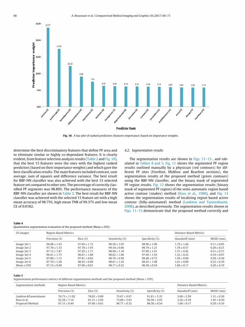

68 A. Boussouar et al. / Computerized Medical Imaging and Graphics 56 (2017) 60–73

tures

dtetpbaffsRcmC

TQ

TS

Fig. 10. A bar plot of ranked predictors (fea

etermine the best discriminatory features that define PF area ando eliminate similar or highly co-dependant features. It is clearlyvident, from feature selection analysis results (Table 2 and Fig. 10),hat the best 15 features were the ones with the highest rankedredictors (based on their importance weights) and which gave theest classification results. The main features included contrast, sumverage, sum of squares and difference variance. The best resultor RBF-NN classifier was also achieved with the best 15 selectedeature set compared to other sets. The percentage of correctly clas-ified PF segments was 98.80%. The performance measures of theBF-NN classifier are shown in Table 3. The best result for RBF-NNlassifier was achieved with the selected 15 feature set with a high

ean accuracy of 98.75%, high mean TNR of 99.37% and low mean

E of 0.0182.

able 4uantitative segmentation evaluation of the proposed method (Mean ± STD).

US images Region-Based Metrics

Precision (%) Dice (%) Sensitivity (%

Image Set 1 96.98 ± 1.43 97.69 ± 1.72 98.50 ± 1.05

Image Set 2 97.70 ± 1.33 97.78 ± 1.93 99.34 ± 0.66

Image Set 3 97.13 ± 1.87 97.29 ± 1.71 98.90 ± 1.10

Image Set 4 96.41 ± 1.75 96.61 ± 1.60 98.62 ± 1.06

Image Set 5 97.00 ± 1.13 97.81 ± 0.82 98.76 ± 0.58

Image Set 6 97.70 ± 1.20 98.43 ± 0.96 98.61 ± 1.43

Mean ± STD 97.15 ± 0.49 97.60 ± 0.61 98.77 ± 0.32

able 5egmentation performance metrics of different segmentation methods and the proposed

Segmentation methods Region-Based Metrics

Precision (%) Dice (%) Sensiti

Lankton &Tannenbaum 76.73 ± 11.02 78.02 ± 9.89 75.67 ±Kass et al. 92.28 ± 7.14 81.21 ± 2.95 73.00 ±Proposed Method 97.15 ± 0.49 97.60 ± 0.61 98.77 ±

importance) based on importance weights.

4.2. Segmentation results

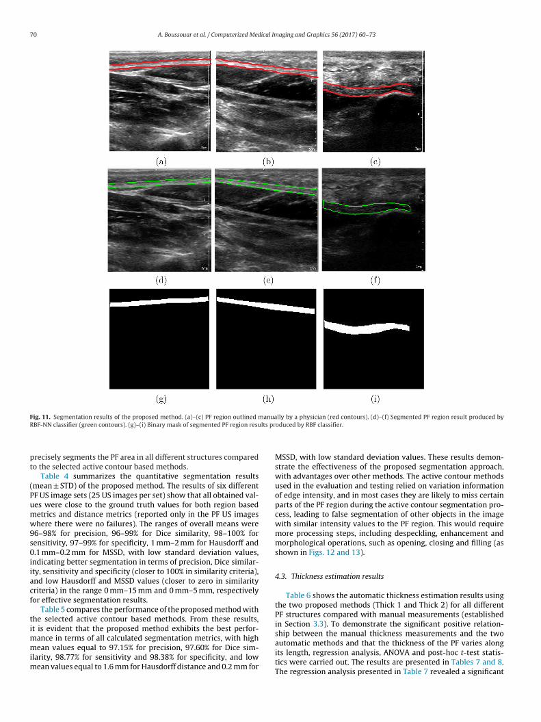
The segmentation results are shown in Figs. 11–13 , and tab-ulated in Tables 4 and 5. Fig. 11 shows the segmented PF regionresults outlined manually by a physician (red contours) for dif-ferent PF sites (Forefoot, Midfoor and Rearfoot sections), thesegmentation results of the proposed method (green contours)using the RBF-NN classifier, and the binary mask of segmentedPF region results. Fig. 12 shows the segmentation results (binarymask of segmented PF region) of the semi-automatic region basedactive contour (snakes) method (Kass et al., 1988), and Fig. 13shows the segmentation results of localizing region based active

contour (fully-automated) method (Lankton and Tannenbaum,2008), as described previously. The segmentation results shown inFigs. 11–13 demonstrate that the proposed method correctly and

Distance-Based Metrics

) Specificity (%) Hausdorff (mm) MSSD (mm)

98.90 ± 1.06 1.79 ± 1.66 0.11 ± 0.0598.79 ± 1.21 1.78 ± 0.57 0.20 ± 0.2197.99 ± 1.01 1.57 ± 0.42 0.31 ± 0.3797.49 ± 1.93 1.32 ± 0.25 0.10 ± 0.0798.48 ± 0.72 1.56 ± 0.60 0.28 ± 0.3698.43 ± 1.08 1.61 ± 0.89 0.22 ± 0.2998.38 ± 0.54 1.60 ± 0.17 0.20 ± 0.10

method (Mean ± STD).

Distance-Based Metrics

vity (%) Specificity (%) Hausdorff (mm) MSSD (mm)

9.97 91.81 ± 5.35 3.00 ± 2.59 1.31 ± 0.30 5.93 96.58 ± 3.95 2.26 ± 0.18 1.45 ± 0.50

0.32 98.38 ± 0.54 1.60 ± 0.17 0.20 ± 0.10

A.

Boussouar et

al. /

Computerized

Medical

Imaging

and G

raphics 56

(2017) 60–73

69

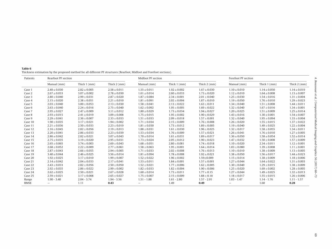
Table 6Thickness estimation by the proposed method for all different PF structures (Rearfoot, Midfoot and Forefoot sections).

Patients Rearfoot PF section Midfoot PF section Forefoot PF section

Manual (mm) Thick 1 (mm) Thick 2 (mm) Manual (mm) Thick 1 (mm) Thick 2 (mm) Manual (mm) Thick 1 (mm) Thick 2 (mm)

Case 1 2.49 ± 0.030 2.82 ± 0.005 2.58 ± 0.011 1.55 ± 0.011 1.92 ± 0.002 1.67 ± 0.030 1.10 ± 0.010 1.14 ± 0.050 1.14 ± 0.019Case 2 2.67 ± 0.033 3.07 ± 0.002 2.78 ± 0.030 1.61 ± 0.014 2.60 ± 0.033 1.73 ± 0.020 1.12 ± 0.010 1.64 ± 0.008 1.13 ± 0.007Case 3 2.80 ± 0.040 2.99 ± 0.031 2.87 ± 0.020 1.87 ± 0.084 2.34 ± 0.001 2.01 ± 0.040 1.25 ± 0.030 1.54 ± 0.016 1.31 ± 0.004Case 4 2.15 ± 0.020 2.38 ± 0.051 2.21 ± 0.010 1.81 ± 0.091 2.02 ± 0.004 1.87 ± 0.010 1.19 ± 0.050 1.76 ± 0.010 1.29 ± 0.023Case 5 2.03 ± 0.040 3.00 ± 0.053 2.13 ± 0.030 1.58 ± 0.041 2.13 ± 0.022 1.63 ± 0.011 1.34 ± 0.040 1.51 ± 0.008 1.44 ± 0.011Case 6 2.63 ± 0.040 2.24 ± 0.016 2.75 ± 0.040 1.62 ± 0.092 1.95 ± 0.005 1.69 ± 0.022 1.32 ± 0.040 1.67 ± 0.016 1.34 ± 0.001Case 7 2.95 ± 0.027 2.47 ± 0.009 3.11 ± 0.012 1.80 ± 0.029 1.73 ± 0.034 1.94 ± 0.027 1.20 ± 0.025 1.51 ± 0.009 1.25 ± 0.014Case 8 2.93 ± 0.015 2.41 ± 0.019 3.09 ± 0.008 1.75 ± 0.015 1.95 ± 0.002 1.90 ± 0.029 1.43 ± 0.016 1.30 ± 0.001 1.54 ± 0.007Case 9 2.29 ± 0.041 2.36 ± 0.007 2.33 ± 0.033 1.51 ± 0.033 2.09 ± 0.018 1.57 ± 0.001 1.32 ± 0.040 1.95 ± 0.094 1.33 ± 0.004Case 10 1.90 ± 0.035 3.17 ± 0.021 1.94 ± 0.002 1.71 ± 0.034 2.15 ± 0.009 1.76 ± 0.008 1.26 ± 0.020 1.55 ± 0.015 1.37 ± 0.022Case 11 2.21 ± 0.036 2.50 ± 0.033 2.23 ± 0.019 1.81 ± 0.030 1.73 ± 0.012 1.89 ± 0.005 1.19 ± 0.040 1.49 ± 0.025 1.22 ± 0.004Case 12 2.16 ± 0.045 2.82 ± 0.056 2.19 ± 0.013 1.88 ± 0.031 1.61 ± 0.030 1.96 ± 0.025 1.32 ± 0.017 1.58 ± 0.055 1.34 ± 0.011Case 13 2.20 ± 0.041 2.86 ± 0.033 2.23 ± 0.039 1.53 ± 0.034 1.76 ± 0.009 1.57 ± 0.021 1.26 ± 0.041 1.76 ± 0.010 1.27 ± 0.005Case 14 2.86 ± 0.042 2.82 ± 0.021 3.07 ± 0.043 1.70 ± 0.014 1.61 ± 0.031 1.89 ± 0.017 1.36 ± 0.050 1.58 ± 0.054 1.52 ± 0.014Case 15 2.75 ± 0.035 3.19 ± 0.020 2.95 ± 0.031 1.73 ± 0.024 2.05 ± 0.012 1.90 ± 0.023 1.47 ± 0.032 1.50 ± 0.008 1.57 ± 0.009Case 16 2.65 ± 0.065 3.74 ± 0.003 2.69 ± 0.043 1.68 ± 0.051 2.80 ± 0.081 1.74 ± 0.018 1.10 ± 0.020 2.34 ± 0.011 1.12 ± 0.001Case 17 2.68 ± 0.052 2.22 ± 0.009 2.77 ± 0.061 1.58 ± 0.063 1.95 ± 0.001 1.64 ± 0.014 1.03 ± 0.080 1.39 ± 0.008 1.11 ± 0.001Case 18 2.87 ± 0.043 2.66 ± 0.055 2.94 ± 0.005 1.71 ± 0.033 2.02 ± 0.008 1.76 ± 0.013 1.10 ± 0.010 1.38 ± 0.009 1.13 ± 0.005Case 19 3.40 ± 0.044 2.46 ± 0.025 3.56 ± 0.014 1.81 ± 0.094 1.78 ± 0.008 1.92 ± 0.021 1.38 ± 0.050 1.56 ± 0.017 1.44 ± 0.023Case 20 1.92 ± 0.025 3.17 ± 0.010 1.99 ± 0.007 1.52 ± 0.022 1.96 ± 0.002 1.59±0.009 1.15 ± 0.014 1.38 ± 0.009 1.18 ± 0.006Case 21 2.14 ± 0.042 2.04 ± 0.033 2.17 ± 0.041 1.53 ± 0.011 1.84 ± 0.001 1.57 ± 0.001 1.27 ± 0.044 1.64 ± 0.022 1.31 ± 0.003Case 22 2.43 ± 0.033 2.82 ± 0.056 2.50 ± 0.050 1.52 ± 0.021 1.77 ± 0.006 1.62 ± 0.005 1.30 ± 0.040 1.29 ± 0.015 1.38 ± 0.009Case 23 2.92 ± 0.035 2.86 ± 0.022 2.99 ± 0.002 1.82 ± 0.033 1.82 ± 0.004 1.90 ± 0.006 1.25 ± 0.020 1.69 ± 0.002 1.28 ± 0.005Case 24 2.62 ± 0.025 2.50 ± 0.021 2.67 ± 0.028 1.60 ± 0.014 1.73 ± 0.011 1.77 ± 0.15 1.27 ± 0.044 1.49 ± 0.025 1.32 ± 0.013Case 25 2.59 ± 0.021 3.17 ± 0.008 2.65 ± 0.027 1.75 ± 0.007 2.15 ± 0.009 1.88 ± 0.18 1.18 ± 0.017 1.55 ± 0.015 1.26 ± 0.006Range 1.90 - 3.40 2.04 - 3.74 1.94 - 3.56 1.51 - 1.88 1.61 - 2.80 1.57 - 2.01 1.03 - 1.47 1.14 - 1.76 1.11 - 1.57RMSE — 1.11 0.43 — 1.49 0.49 — 1.60 0.28

70 A. Boussouar et al. / Computerized Medical Imaging and Graphics 56 (2017) 60–73

Fig. 11. Segmentation results of the proposed method. (a)–(c) PF region outlined manually by a physician (red contours). (d)–(f) Segmented PF region result produced byR lts pr

pt

(Pumw9s0iiacf

timmim

BF-NN classifier (green contours). (g)–(i) Binary mask of segmented PF region resu

recisely segments the PF area in all different structures comparedo the selected active contour based methods.

Table 4 summarizes the quantitative segmentation resultsmean ± STD) of the proposed method. The results of six differentF US image sets (25 US images per set) show that all obtained val-es were close to the ground truth values for both region basedetrics and distance metrics (reported only in the PF US imageshere there were no failures). The ranges of overall means were

6–98% for precision, 96–99% for Dice similarity, 98–100% forensitivity, 97–99% for specificity, 1 mm–2 mm for Hausdorff and.1 mm–0.2 mm for MSSD, with low standard deviation values,

ndicating better segmentation in terms of precision, Dice similar-ty, sensitivity and specificity (closer to 100% in similarity criteria),nd low Hausdorff and MSSD values (closer to zero in similarityriteria) in the range 0 mm–15 mm and 0 mm–5 mm, respectivelyor effective segmentation results.

Table 5 compares the performance of the proposed method withhe selected active contour based methods. From these results,t is evident that the proposed method exhibits the best perfor-

ance in terms of all calculated segmentation metrics, with highean values equal to 97.15% for precision, 97.60% for Dice sim-

larity, 98.77% for sensitivity and 98.38% for specificity, and lowean values equal to 1.6 mm for Hausdorff distance and 0.2 mm for

oduced by RBF classifier.

MSSD, with low standard deviation values. These results demon-strate the effectiveness of the proposed segmentation approach,with advantages over other methods. The active contour methodsused in the evaluation and testing relied on variation informationof edge intensity, and in most cases they are likely to miss certainparts of the PF region during the active contour segmentation pro-cess, leading to false segmentation of other objects in the imagewith similar intensity values to the PF region. This would requiremore processing steps, including despeckling, enhancement andmorphological operations, such as opening, closing and filling (asshown in Figs. 12 and 13).

4.3. Thickness estimation results

Table 6 shows the automatic thickness estimation results usingthe two proposed methods (Thick 1 and Thick 2) for all differentPF structures compared with manual measurements (establishedin Section 3.3). To demonstrate the significant positive relation-ship between the manual thickness measurements and the two

automatic methods and that the thickness of the PF varies alongits length, regression analysis, ANOVA and post-hoc t-test statis-tics were carried out. The results are presented in Tables 7 and 8.The regression analysis presented in Table 7 revealed a significant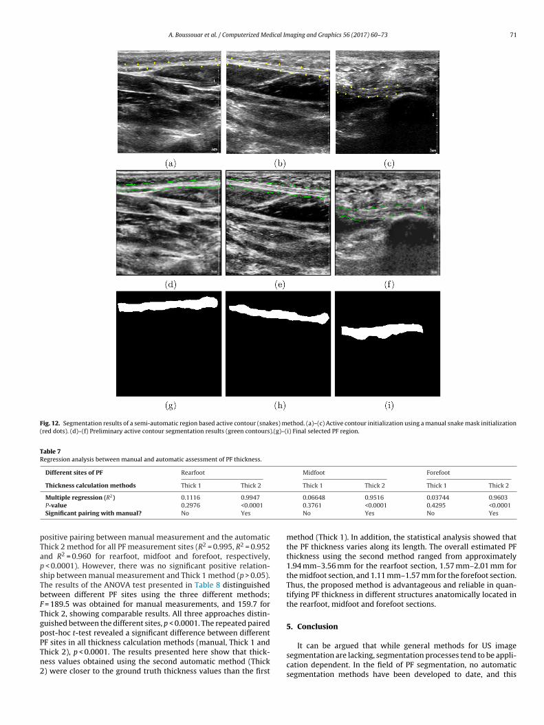

A. Boussouar et al. / Computerized Medical Imaging and Graphics 56 (2017) 60–73 71

Fig. 12. Segmentation results of a semi-automatic region based active contour (snakes) method. (a)–(c) Active contour initialization using a manual snake mask initialization(red dots). (d)–(f) Preliminary active contour segmentation results (green contours).(g)–(i) Final selected PF region.

Table 7Regression analysis between manual and automatic assessment of PF thickness.

Different sites of PF Rearfoot Midfoot Forefoot

Thickness calculation methods Thick 1 Thick 2 Thick 1 Thick 2 Thick 1 Thick 2

2

pTapsTbFTgpPTn2

Multiple regression (R ) 0.1116 0.9947

P-value 0.2976 <0.0001

Significant pairing with manual? No Yes

ositive pairing between manual measurement and the automatichick 2 method for all PF measurement sites (R2 = 0.995, R2 = 0.952nd R2 = 0.960 for rearfoot, midfoot and forefoot, respectively,

< 0.0001). However, there was no significant positive relation-hip between manual measurement and Thick 1 method (p > 0.05).he results of the ANOVA test presented in Table 8 distinguishedetween different PF sites using the three different methods;

= 189.5 was obtained for manual measurements, and 159.7 forhick 2, showing comparable results. All three approaches distin-uished between the different sites, p < 0.0001. The repeated pairedost-hoc t-test revealed a significant difference between different

F sites in all thickness calculation methods (manual, Thick 1 andhick 2), p < 0.0001. The results presented here show that thick-ess values obtained using the second automatic method (Thick) were closer to the ground truth thickness values than the first

0.06648 0.9516 0.03744 0.96030.3761 <0.0001 0.4295 <0.0001No Yes No Yes

method (Thick 1). In addition, the statistical analysis showed thatthe PF thickness varies along its length. The overall estimated PFthickness using the second method ranged from approximately1.94 mm–3.56 mm for the rearfoot section, 1.57 mm–2.01 mm forthe midfoot section, and 1.11 mm–1.57 mm for the forefoot section.Thus, the proposed method is advantageous and reliable in quan-tifying PF thickness in different structures anatomically located inthe rearfoot, midfoot and forefoot sections.

5. Conclusion

It can be argued that while general methods for US imagesegmentation are lacking, segmentation processes tend to be appli-cation dependent. In the field of PF segmentation, no automaticsegmentation methods have been developed to date, and this

72 A. Boussouar et al. / Computerized Medical Imaging and Graphics 56 (2017) 60–73

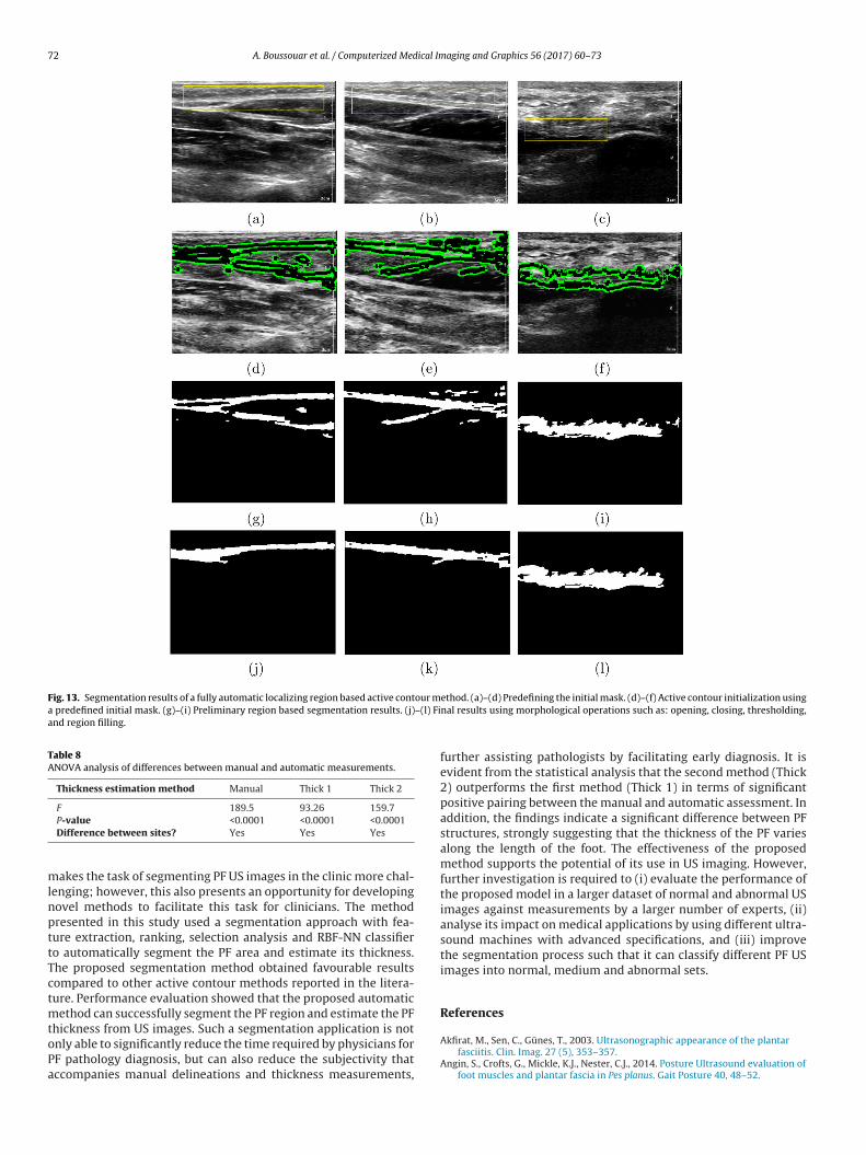
Fig. 13. Segmentation results of a fully automatic localizing region based active contour ma predefined initial mask. (g)–(i) Preliminary region based segmentation results. (j)–(l) Fiand region filling.

Table 8ANOVA analysis of differences between manual and automatic measurements.

Thickness estimation method Manual Thick 1 Thick 2

F 189.5 93.26 159.7

mlnpttTctmtoPa

P-value <0.0001 <0.0001 <0.0001Difference between sites? Yes Yes Yes

akes the task of segmenting PF US images in the clinic more chal-enging; however, this also presents an opportunity for developingovel methods to facilitate this task for clinicians. The methodresented in this study used a segmentation approach with fea-ure extraction, ranking, selection analysis and RBF-NN classifiero automatically segment the PF area and estimate its thickness.he proposed segmentation method obtained favourable resultsompared to other active contour methods reported in the litera-ure. Performance evaluation showed that the proposed automatic

ethod can successfully segment the PF region and estimate the PF

hickness from US images. Such a segmentation application is notnly able to significantly reduce the time required by physicians forF pathology diagnosis, but can also reduce the subjectivity thatccompanies manual delineations and thickness measurements,

ethod. (a)–(d) Predefining the initial mask. (d)–(f) Active contour initialization usingnal results using morphological operations such as: opening, closing, thresholding,

further assisting pathologists by facilitating early diagnosis. It isevident from the statistical analysis that the second method (Thick2) outperforms the first method (Thick 1) in terms of significantpositive pairing between the manual and automatic assessment. Inaddition, the findings indicate a significant difference between PFstructures, strongly suggesting that the thickness of the PF variesalong the length of the foot. The effectiveness of the proposedmethod supports the potential of its use in US imaging. However,further investigation is required to (i) evaluate the performance ofthe proposed model in a larger dataset of normal and abnormal USimages against measurements by a larger number of experts, (ii)analyse its impact on medical applications by using different ultra-sound machines with advanced specifications, and (iii) improvethe segmentation process such that it can classify different PF USimages into normal, medium and abnormal sets.

References

Akfirat, M., Sen, C., Günes, T., 2003. Ultrasonographic appearance of the plantarfasciitis. Clin. Imag. 27 (5), 353–357.

Angin, S., Crofts, G., Mickle, K.J., Nester, C.J., 2014. Posture Ultrasound evaluation offoot muscles and plantar fascia in Pes planus. Gait Posture 40, 48–52.

ical Im

B

B

B

B

B

C

C

C

C

C

C

C

D

D

D

F

G

G

G

H

H

H

H

K

K

K

K

measures for terrain classification. IEEE Trans. Syst. Man Cybern. SMC-6 (4),269–285.

A. Boussouar et al. / Computerized Med

ishop, C.M., 2006. Pattern Recognition and Machine Learning. Springer, New York,USA.

lum, H., 1967. A transformation for extracting new descriptors of dhape. In:Wathen-Dunn, W. (Ed.), Models for the Perception of Speech and Visual Form.MIT Press, Cambridge, MA, USA, pp. 362–380.

ors , A.G., Pitas, I., 1996. Median radial basis function neural network. IEEE Trans.Neural Netw. 7 (6), 1351–1364.

ors, A.G., Pitas, I., 1999. Object classification in 3-d images using alpha-trimmedmean radial basis function network. IEEE Trans. Image Process. 8 (12),1744–1756.

roomhead, D.S., Lowe, D., 1988. Radial basis functions, multi-variable functionalinterpolation and adaptive networks. Tech. rep., Royal Signals and RadarEstablishment, Memorandum No. 4148, London, UK.

han, T., Vese, L., 2001. Active contours without edges. IEEE Trans. Image Process.10 (2), 266–277.

hang, C.-Y., Lei, Y.-F., Tseng, C.-H., Shih, S.-R., 2010. Thyroid segmentation andvolume estimation in ultrasound images. IEEE Trans. Biomed. Eng. 57 (6),1348–1357.

hang, R., 2010. Plantar fasciitis: Biomechanics, atrophy and muscle energetics(PhD dissertation). University of Massachusetts Amherst, USA.

hang, S., Yu, B., Vetterli, M., 2000. Adaptive wavelet thresholding for imagedenoising and compression. IEEE Trans. Image Process. 9 (9), 1532–1546.

heng, J.-W., Tsai, W.-C., Yu, T.-Y., Huang, K.-Y., 2012. Reproducibility ofsonographic measurement of thickness and echogenicity of the plantar fascia.J. Clin. Ultrasound 40 (1), 14–19.

hun, Y.D., Seo, S.Y., Kim, N.C., 2003. Image retrieval using BDIP and BVLCmoments. IEEE Trans. Circuits Syst. Video Technol. 13 (9), 951–957.

rofts, G., Angin, S., Mickle, K.J., Hill, S., Nester, C.J., 2014. Reliability of ultrasoundfor measurement of selected foot structures. Gait Posture 39 (1), 35–39.

eshpande, R., Ramalingam, R., Chockalingam, N., Naemi, R., Branthwaite, H.,Sundar, L., 2013. An automated segmentation technique for the processing offoot ultrasound images. 2013 IEEE Eighth International Conference onIntelligent Sensors, Sensor Networks and Information Processing, 380–383.

i Stefano, L., Bulgarelli, A., 1999. A simple and efficient connected componentslabeling algorithm. In: 1999. Proceedings. International Conference on ImageAnalysis and Processing. IEEE, pp. 322–327.

ice, L.R., 1945. Measures of the amount of ecologic association between species.Ecology 26 (3), 297–302.

abrikant, J.M., Park, T.S., 2011. Plantar fasciitis (fasciosis) treatment outcomestudy: plantar fascia thickness measured by ultrasound and correlated withpatient self-reported improvement. Foot 21 (2), 79–83.

anzalez, R.C., Woods, R.E., 2002. Digital Image Processing, 2nd ed. Prentice-Hall,Englewood Cliffs, NJ, USA.

onzalez, R., Woods, R., 2011. Digital Image Processing. Pearson Education Asia,India.

onzalez, R., Woods, R., Eddins, S., 2010. Digital Image Processing Using MATLAB.Tata McGraw Hill Education, Private Limited, New Delhi, India.

am, F.M., Kostanic, I., 2000. Principles of Neurocomputing for Science andEngineering, 1st Edition. McGraw-Hill Higher Education, Private Limited, NewDelhi, India.

aralick, R.M., Shanmugam, K., Dinstein, I.H., 1973. Textural features for imageclassification. IEEE Trans. Syst. Man Cybern. SMC-3 (6), 610–621.

eimann, T., Van Ginneken, B., Styner, M., Arzhaeva, Y., Aurich, V., Bauer, C., Beck,A., Becker, C., Beichel, R., Bekes, G., et al., 2009. Comparison and evaluation ofmethods for liver segmentation from ct datasets. IEEE Trans. Med. Imag. 28 (8),1251–1265.

uang, C.-K., Kitaoka, H.B., An, K.-N., Chao, E.Y., 1993. Biomechanical evaluation oflongitudinal arch stability. Foot Ankle Int. 14 (6), 353–357.

ass, M., Witkin, A., Terzopoulos, D., 1988. Snakes: active contour models. Int. J.Comput. Vis. 1 (4), 321–331.

elikian, A.S., 2012. Sarrafian’s Anatomy of the Foot and Ankle: Descriptive,Topographic, Functional. Lippincott Williams & Wilkins, Philadelphia, USA.

ingsbury, N., 1998. The dual-tree complex wavelet transform: a new technique

for shift invariance and directional filters. In: Proceeding of the 8th IEEE DSPWorkshop, Utah. Vol. 8. Citeseer, p. 86.

ingsbury, N., 1999. Shift invariant properties of the dual-tree complex wavelettransform. Proceedings of the 1999 IEEE International Conference onAcoustics, Speech and Signal Processing, vol. 3.

aging and Graphics 56 (2017) 60–73 73

Kwong, P., Kay, D., Voner, R., White, M., 1988. Plantar fasciitis. mechanics andpathomechanics of treatment. Clin. Sports Med. 7 (1), 119–126.

Lankton, S., Tannenbaum, A., 2008. Localizing region-based active contours. IEEETrans. Image Process. 17 (11), 1–11.

Moody, J., Darken, C.J., 1989. Fast learning in networks of locally-tuned processingunits. Neural Comput. 1 (2), 281–294.

Noble, J.A., Boukerroui, D., 2006. Ultrasound image segmentation: A survey. IEEETrans. Med. Imag. 25 (8), 987–1010.

Orr, M.J.L., 1996. Introduction to Radial Basis Function Networks.Park, J.W., Yoon, K., Chun, K.S., Lee, J.Y., Park, H.J., Lee, S.Y., Lee, Y.T., 2014.

Long-term outcome of low-energy extracorporeal shock wave therapy forplantar fasciitis: Comparative analysis according to ultrasonographic findings.Ann. Rehabil. Med. 38 (4), 534–540.

Pizer, S.M., Amburn, E.P., Austin, J.D., Cromartie, R., Geselowitz, A., Greer, T., terHaar Romeny, B., Zimmerman, J.B., Zuiderveld, K., 1987. Adaptive histogramequalization and its variations. Comput. Vis. Graphics Image Process. 39 (3),355–368.

Pope, J.A., 1999. Medical Physics: Imaging. Heinemann Advanced Science. PearsonEducation Limited, Harlow, UK.

Roffo, G., Melzi, S., Cristani, M., 2015. Infinite feature selection. 2015 IEEEInternational Conference on Computer Vision (ICCV), 4202–4210.

Rubinstein, R.Y., 1997. Optimization of computer simulation models with rareevents. Eur. J. Oper. Res. 99 (1), 89–112.

Rueda, S., Fathima, S., Knight, C.L., Yaqub, M., Papageorghiou, A.T., Rahmatullah, B.,Foi, A., Maggioni, M., Pepe, A., Tohka, J., Stebbing, R.V., McManigle, J.E., Ciurte,A., Bresson, X., Cuadra, M.B., Sun, C., Ponomarev, G.V., Gelfand, M.S., Kazanov,M.D., Wang, C.-W., Chen, H.-C., Peng, C.-W., Hung, C.-M., Noble, J.A., 2014.Evaluation and comparison of current fetal ultrasound image segmentationmethods for biometric measurements: a grand challenge. IEEE Trans. Med.Imag. 33 (4), 797–813.

Saber, N., Diab, H., Nassar, W., Razaak, H.A., 2012. Ultrasound guided local steroidinjection versus extracorporeal shockwave therapy in the treatment of plantarfasciitis. Alexandria J. Med. 48 (1), 35–42.

Selesnick, I., Baraniuk, R., Kingsbury, N., 2005. The dual-tree complex wavelettransform. IEEE Signal Process. Mag. 22 (6), 123–151.

Sendur, L., Selesnick, I., 2002. Bivariate shrinkage functions for wavelet-baseddenoising exploiting interscale dependency. IEEE Trans. Signal Process. 50 (11),2744–2756.

Shih, F., 2009. Image Processing and Mathematical Morphology: Fundamentals andApplications. CRC Press, Taylor & Francis, Boca Raton, USA.

Sokolova, M., Lapalme, G., 2009. A systematic analysis of performance measuresfor classification tasks. Inf. Process. Manag. 45 (4), 427–437.

Szabo, T.L., 2013. Diagnostic Ultrasound Imaging: Inside Out. BiomedicalEngineering. Elsevier Science Academic Press, Cambridge, Massachusetts, USA.

Telea, A., 2014. Data Visualization: Principles and Practice, 2nd ed. Taylor &Francis, Milton Park, Abingdon, UK.

Udupa, J.K., Leblanc, V.R., Zhuge, Y., Imielinska, C., Schmidt, H., Currie, L.M., Hirsch,B.E., Woodburn, J., 2006. A framework for evaluating image segmentationalgorithms. Comput. Med. Imaging Graph. 30 (2), 75–87.

Umbaugh, S., 2005. Computer Imaging: Digital Image Analysis and Processing. ACRC Press Book. Taylor & Francis, Milton Park, Abingdon, UK.

Wearing, S.C., Smeathers, J.E., Sullivan, P.M., Yates, B., Urry, S.R., Dubois, P., 2007.Plantar fasciitis: are pain and fascial thickness associated with arch shape andloading? Phys. Ther. 87 (8), 1002–1008.

Wearing, S.C., Smeathers, J.E., Yates, B., Sullivan, P.M., Urry, S.R., Dubois, P., 2004.Sagittal movement of the medial longitudinal arch is unchanged in plantarfasciitis. Med. Sci. Sports Exerc. 36 (10), 1761–1767.

Wen, X., Yuan, H., Yang, C., Song, C., Duan, B., Zhao, H., 2007. Improved haarwavelet feature extraction approaches for vehicle detection. In: IntelligentTransportation Systems Conference, ITSC 2007, IEEE, pp. 1050–1053.

Weszka, J.S., Dyer, C.R., Rosenfeld, A., 1976. A comparative study of texture

Zuiderveld, K., 1994. Graphi gems IV. In: Contrast limited adaptive histogramequalization. Academic Press Professional, Inc., San Diego, CA, USA, pp.474–485.