PLANT LEAF IDENTIFICATION USING MOMENT INVARIANTS

& GENERAL REGRESSION NEURAL NETWORK

ZALIKHA BT ZULKIFLI

UNIVERSITI TEKNOLOGI MALAYSIA

PLANT LEAF IDENTIFICATION USING MOMENT INVARIANTS

& GENERAL REGRESSION NEURAL NETWORK

ZALIKHA BT ZULKIFLI

A project report submitted in partial fulfillment of the

requirements for the award of the degree of

Master of Science (Computer Science)

Faculty of Computer Science and Information Systems

Universiti Teknologi Malaysia

OCTOBER 2009

iii

To my beloved Mama and Baba,

for letting me exprience the kind of love

that people freely die for.

And also to my sisters and Noor Hafizzul,

for your patience, love, friendship and humor.

iv

ACKNOWLEDGEMENTS

All praises and gratitude to Allah s.w.t, who has guided and blessed me in

finishing my project successfully.

In the first place I would like to record my gratitude to Assoc. Prof. Dr. Puteh

Saad for her supervision, advice and guidance from the very early to the final stage

of this project which enabled me to develop an understanding of this project. Her

involvement has triggered and nourished my intellectual maturity that I will benefit

from, for a long time to come.

Words fail me to express my appreciation to my parents for their dedication,

love, inseparable support and prayers. To my sisters, Shazana, Amira, Diyana and

Nur Alia, thank you for being supportive and caring siblings.

My special thanks goes to my friends, Hafizz, Umie, Ekin and Huda for their

warm support and encouragement, each from unique perspective. To others who

have assisted in any way, I express my sincere gratitude.

Finally, I would like to thank everbody who was important to the completion

of the project, as well as expressing my apology that I could not mention personally

one by one.

v

ABSTRACT

Living plant identification based on images of leaf is a very challenging task

in the field of pattern recognition and computer vision. However, leaf classification

is an important component of computerized living plant recognition. As inherent

trait, leaf definitely contains important information for plant species identification

despite its complexity. The objective of this research is to identify the effectiveness

of three moment invariant methods, namely Zernike Moment Invariant (ZMI),

Legendre Moment Invariant (LMI) and Tchebichef Moment Invariant (TMI) to

extract features from plant leaf images. Then, the resulting set of features

representing the leaf images are classified using General Regression Neural Network

(GRNN) for recognition purposes. There are two main stages involved in plant leaf

identification. The first stage is known as feature extraction process where moment

invariant methods are applied. The output of this process is a set of a global vector

feature that represents the shape of the leaf images. It is shown that TMI can extract

vector feature with Percentage of Absolute Error (PAE) less than 10.38 percent.

Therefore, TMI vector feature will be the input to second stage. The second stage

involves classification of leaf images based on the derived feature gained in the

previous stage. It is found that GRNN classifier produces 100 percent classification

rate with average computational time of 0.47 seconds.

vi

ABSTRAK

Pengenalpastian tumbuh-tumbuhan berdasarkan imej daun adalah satu tugas

yang sangat mencabar dalam bidang pengecaman pola. Walaubagaimanapun,

pengelasan daun adalah salah satu komponen yang penting dalam pengecaman

tumbuh-tumbuhan secara berkomputer. Berdasarkan ciri-ciri yang diwarisi, daun

mengandungi maklumat penting untuk pengecaman spesis tumbuhan walaupun

terdapat ciri-cirinya yang rumit. Kajian ini bertujuan untuk mengenalpasti

keberkesanan tiga teknik momen tak varian, iaitu Zernike Moment Invariant (ZMI),

Legendre Moment Invariant (LMI) and Tchebichef Moment Invariant (TMI) dalam

pengekstrakan fitur. Kemudian, hasil daripada pengekstrakan fitur imej daun

dikelaskan menggunakan pengelas General Regression Neural Network (GRNN)

bagi tujuan pengecaman. Terdapat dua fasa utama yang terlibat dalam pengecaman

daun. Fasa pertama dikenali sebagai proses pengestrakan fitur di mana teknik

momen tak varian digunakan. Ouput yang dihasilkan daripada proses ini adalah set

vektor fitur sejagat yang mewakili bentuk imej daun. Didapati bahawa TMI dapat

mengestrak fitur dengan peratus ralat (PAE) kurang daripada 10.38 peratus. Oleh itu,

vektor fitur daripada TMI akan dijadikan sebagai input pada fasa kedua. Fasa kedua

melibatkan pengelasan imej daun. Didapati bahawa pengelas GRNN mempunyai

jumlah klasifikasi paling tepat (100 peratus) dengan purata masa menumpu 0.47 saat.

vii

TABLE OF CONTENTS

CHAPTER TITLE PAGE

DECLARATION ii

DEDICATION iii

ACKNOWLEDGEMENTS iv

ABSTRACT v

ABSTRAK vi

TABLE OF CONTENTS vii

LIST OF TABLES xi

LIST OF FIGURES xiii

LIST OF ABBREVIATIONS xv

LIST OF APPENDICES xvi

1 INTRODUCTION 1

1.1 Introduction 1

1.2 Problem Background 3

1.3 Problem Statement 4

1.4 Importance of the Study 4

1.5 Objectives of the Project 5

1.6 Scopes of the Project 6

1.7 Summary 6

viii

2 LITERATURE REVIEW 7

2.1 Introduction 7

2.2 Moment Invariants 9

2.2.1 Zernike Moment Invariant 11

2.2.2 Legendre Moment Invariant 13

2.2.3 Tchebichef Moment Invariant 15

2.3 Implementation of Moment Invariant in

Pattern Recognition Applications 16

2.3.1 Face Recognition 17

2.3.2 Optical Character Recognition 18

2.3.3 Other Pattern Recognition Applications 19

2.4 Artificial Neural Networks 21

2.4.1 General Regression Neural Networks 21

2.5 Neural Networks Implementation 24

2.6 Summary 25

3 METHODOLOGY 26

3.1 Introduction 26

3.2 Research Framework 27

3.3 Software Requirement 28

3.4 Image Source 28

3.5 Image Pre-processing 29

3.6 Feature Extraction 30

3.6.1 ZMI Algorithm 31

3.6.2 LMI Algorithm 33

3.6.3 TMI Algorithm 34

3.7 Intra-class Analysis 35

3.8 Inter-class Analysis 37

3.9 Data Pre-processing 38

3.10 Classification by Neural Networks 39

3.11 Inter-class Analysis 40

3.12 Summary 42

ix

4 IMPLEMENTATION, COMPARISON OF

RESULTS AND DISCUSSION 43

4.1 Introduction 43

4.2 Leaf Images 44

4.3 Result of Intra-class Analysis 46

4.3.1 Absolute Error 48

4.3.2 Percentage Absolute Error (PAE) 50

4.3.3 Percentage Min Absolute Error 1

(PMAE1) 52

4.3.4 Percentage Min Absolute Error 2

(PMAE2) 53

4.3.5 Total Percentage Mean Absolute

Error (TPMAE) 54

4.4 Result of Inter-class Analysis 55

4.4.1 Comparison Based On Value of

Feature Vectors 55

4.4.2 Comparison Based On Computational

Time 58

4.5 Analysis of Feature Extraction Results 59

4.6 Classification Phase 59

4.6.1 Data Preparation 60

4.6.2 GRNN Spread Parameters Declaration 60

4.7 Classification Results of GRNN Classifier 61

4.8 Summary 64

5 DISCUSSION AND CONCLUSION 65

5.1 Introduction 65

5.2 Discussion of Results 65

5.3 Problems and Limitations of Research 67

5.4 Recommendation for Future Works 67

5.5 Conclusion 68

x

REFERENCES 70

APPENDICES A-H 75 - 96

xi

LIST OF TABLES

TABLE NO. TITLE PAGE

2.1 List of face recognition applications that use moment invariants 17

2.2 List of OCR applications that use moment Invariants 19

2.3 List of other pattern recognition applications that use moment invariants 20

2.4 List of applications that use neural networks as classifier 24

3.1 The value of scaling and rotation factors 30 4.1 List of image name 44 4.2 Scaling and rotation factors of image A1 46 4.3 Value of feature vectors using ZMI 47 4.4 Value of feature vectors using LMI 47 4.5 Value of feature vectors using TMI 48 4.6 Absolute Error for ZMI 49 4.7 Absolute Error for LMI 49 4.8 Absolute Error for TMI 50 4.9 PAE for image A1 with rotate factor of 10° 51 4.10 TPMAE of different moments for image A1 54

xii

4.11 Value of feature vectors of four images for ZMI 56 4.12 Value of feature vectors of four images for LMI 56 4.13 Value of feature vectors of four images for TMI 56 4.14 Computational time taken in seconds 58 4.15 GRNN result for each spread parameters 62

xiii

LIST OF FIGURES

FIGURE NO. TITLE PAGE

2.1 GRNN architecture 23 3.1 Process involve in research framework 27 3.2 Algorithm of Basic_GMI() computation 32 3.3 Algorithm of ZMI computation 32 3.4 Algorithm of Norm() computation 33 3.5 Algorithm of LMI computation 34 3.6 Algorithm of TMI computation 35 3.7 Process of training, validation and testing phase

in neural network 40 4.1 Leaf images 44 4.2 An image A1 with its various rotations and

scaling factor 45 4.3 PAE graph for image A1 with rotate factor of 10° 51 4.4 PMAE1 graph for image A1 with image variation 52 4.5 PMAE2 graph for image A1 with different dimension 53 4.6 TPMAE graph of different moments for image A1 54 4.7 Comparison value of feature vectors based on leaf

class 57

xiv

4.8 Comparison value of feature vectors based on leaf class for original image 57

4.9 k-fold partition of the dataset 60 4.10 Graph of PCC versus spread parameter value 63 4.11 Graph of time average versus spread parameter value 63

xv

LIST OF ABBREVIATIONS

AE – Absolute Error

ANN – Artificial Neural Network

BPN – Back-propagation Neural Network

GMI – Geometric Moment Invariant

GRNN – General Regression Neural Network

IEC – Invariant Error Computation

k-NN – k-nearest neighbor

LMI – Legendre Moment Invariant

MLPN – Multilayer Perceptron Neural Network

MMC – Moving Median Centers

NCC – Number of Correct Classification

OCR – Optical Character Recognition

PAE – Percentage Absolute Error

PCA – Principal Components Analysis

PCC – Percentage of Correct Classification

PMAE1 – Percentage of Mean Absolute Error 1

PNN – Probabilistic Neural Network

RBFNN – Radial Basis Function Neural Network

RBPNN – Radial Basis Probabilistic Neural Network

TIFF – Tagged Image File Format

TMI – Tchebichef Moment Invariant

ZMI – Zernike Moment Invariant

xvi

LIST OF APPENDICES

APPENDIX TITLE PAGE

A Project 1 Gantt Chart 75 B Project 2 Gantt Chart 77

C Original Leaf Images 79 D Binary Leaf Images 81 E Image References 83 F Value of Feature Vectors By ZMI 85 G Value of Feature Vectors By LMI 89 H Value of Feature Vectors By TMI 93

CHAPTER 1

INTRODUCTION

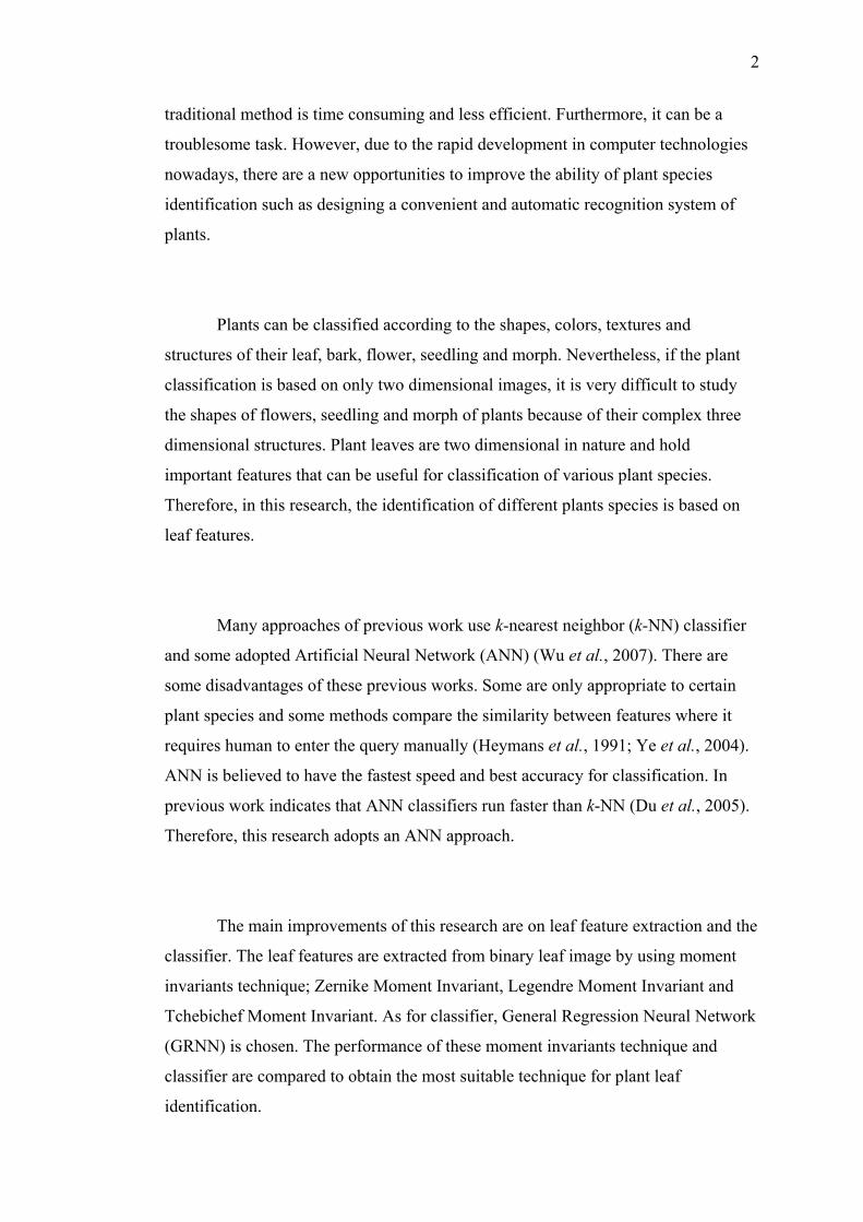
1.1 Introduction

Plant is greatly important sources for human’s living and development

whether in industry, food stuff or medicines. It is also significantly important for

environmental protection. According to World Wide Fund for Nature (WWF), there

are currently about 50, 000 - 70, 000 known species all over the world (WWF,

2007). However, many plant species are still unknown yet and with the deterioration

of environments, these unknown species might be at the margin of extinction. So it

is necessary to correctly and quickly identify the plant species in order to preserve its

genetic resources.

Plant species identification is a process in which each individual plant should

be correctly assigned to descending series of groups of related plants, as based on

common characteristics (Du et al., 2006). Currently, plant taxonomy methods still

adopt traditional classification method such as morphologic anatomy, cell biology

and molecular biological approaches. This task mainly carried out by botanists. The

2

traditional method is time consuming and less efficient. Furthermore, it can be a

troublesome task. However, due to the rapid development in computer technologies

nowadays, there are a new opportunities to improve the ability of plant species

identification such as designing a convenient and automatic recognition system of

plants.

Plants can be classified according to the shapes, colors, textures and

structures of their leaf, bark, flower, seedling and morph. Nevertheless, if the plant

classification is based on only two dimensional images, it is very difficult to study

the shapes of flowers, seedling and morph of plants because of their complex three

dimensional structures. Plant leaves are two dimensional in nature and hold

important features that can be useful for classification of various plant species.

Therefore, in this research, the identification of different plants species is based on

leaf features.

Many approaches of previous work use k-nearest neighbor (k-NN) classifier

and some adopted Artificial Neural Network (ANN) (Wu et al., 2007). There are

some disadvantages of these previous works. Some are only appropriate to certain

plant species and some methods compare the similarity between features where it

requires human to enter the query manually (Heymans et al., 1991; Ye et al., 2004).

ANN is believed to have the fastest speed and best accuracy for classification. In

previous work indicates that ANN classifiers run faster than k-NN (Du et al., 2005).

Therefore, this research adopts an ANN approach.

The main improvements of this research are on leaf feature extraction and the

classifier. The leaf features are extracted from binary leaf image by using moment

invariants technique; Zernike Moment Invariant, Legendre Moment Invariant and

Tchebichef Moment Invariant. As for classifier, General Regression Neural Network

(GRNN) is chosen. The performance of these moment invariants technique and

classifier are compared to obtain the most suitable technique for plant leaf

identification.

3

1.2 Problem Background

Plant is a living form with the largest population and has the widest

distribution on the earth. There are many kinds of plant species living on the earth,

which plays an important part in improving the environment of human life and other

lives existing on the earth. Unfortunately, more and more plant species are at the

margin of extinction. Therefore, it is important to correctly and quickly recognize the

plant species in order to understand and managing them. However, it is difficult for

layman to recognize the plant species and currently, Botanist is the expert. Due to the

limited number of experts, it is very necessary to automatically recognize the

different kind of leaves for plant classification.

Plant classification not only recognizes different plants and names of the

plant but also provides the differences of different plants and builds system for

classifying plant. There have been several approaches for plant classification based

on plant features of leaves, barks and flowers. In this study, the plant classification

will be determined by plant leaf features because the leaf carry useful information

for classification of various plants such as aspect ratio, shape and texture.

This study is to explore the effectiveness of three moment invariants

technique, namely Zernike Moment Invariant (ZMI), Legendre Moment Invariant

(LMI) and Tchebichef Moment Invariant (TMI) for extraction of binary leaf image.

This study also intends to determine the performance of GRNN as classifiers in leaf

recognition. Thus, the finding from this study can provide useful information for

developing automated plant classification tools.

4

1.3 Problem Statement

Feature Extraction and classification are two challenging phases in image

analysis applications. The following are the problem statement for this study:

• There is no general feature extraction technique that is available for all types

of images. Thus, experimentations need to be carried out to determine

among Moment-based techniques, which one of them is most suitable for

plant leaf images.

• An issue that in the classification phase is the matching task since the set

features extracted is numerous for a single image.

1.4 Importance of the Study

This study involves the identification of plant leaf. Many of the existing plant

species on the earth are still unknown, which might be at the margin of extinction.

There are many ways to recognize the plant species, but it usually time consuming.

This is because it involves the expert, botanists to recognize the plant species.

Therefore, it is very important to automatically recognize the plant species in order

to manage them.

It is difficult for layman to recognize plant species. By having a computer-

aided plant identification system, they can also identify the plant species. This will

increase an interest in studying plant taxonomy and ecology, lift biology educations

5

standards and promote the use of information technology for the management of

natural reserve parks and forest plantation.

By doing this research, the best approach for leaf features extraction and

classification have to be analyze. The performance of three moment invariants

technique and the classifiers will be compared to give best results and very high

performance in a short time. Thus, it is important to expand the knowledge of the

study so that it can give benefit for the environmental protection to preserve

endangered plant species.

1.5 Objectives of the Project

i. To compare the effectiveness of three moment invariants techniques, namely

Zernike Moment Invariant (ZMI), Legendre Moment Invariant (LMI) and

Tchebichef Moment Invariant (TMI) to extract features from leaf images.

ii. To classify the set of features representing the leaf images using General

Regression Neural Network (GRNN).

iii. To evaluate the performance of features extraction techniques and the

classifier based on inter- class and intra-class invariance.

6

1.6 Scopes of the Project

i. In this study, the binary plant leaf shape images are used and acquired by

digital camera.

ii. Only three moment invariants techniques, namely ZMI, LMI and TMI are

used for features extraction of binary plant leaf images.

iii. GRNN classifier is utilized for leaf classification.

1.7 Summary

This chapter discussed a general introduction of the potential and challenges

of plant identification. As stated in the chapter, the main objectives of this research is

to determine the effectiveness and performance of each methods used in this

research. Each methods used will be investigate and explore in order to achieved the

objectives and overcome the problems of this research. The next chapter will be the

literature review, where a description of the literature relevant to the research is

presented.

CHAPTER 2

LITERATURE REVIEW

2.1 Introduction

Automatic recognition, classification and grouping of patterns are important

problems in variety of engineering and scientific disciplines such as artificial

intelligence, computer vision, biology and medicine. Interest in the area of plant leaf

recognition has been improved recently due to emerging applications which are not

only challenging, but also computationally demanding. Classification of plants is a

very old field, which is carried out by taxonomists and botanists and it is time

consuming processes. Due to this time consuming process and the fact that the

identification is not trivial for non-experts, it could be helpful if the identification

process is by a computer-based automatic system.

In recent years, several researchers have dedicated their work to plant

identification. Till now, many works have focused on leaf feature extraction for

recognition of plant. In addition, leaf shape is one of the characteristics that play an

important role in the plant leaf classification process and need to be evaluated. Wang

8

X. F., et al. (2005) introduced a method of recognizing leaf images based on shape

features using hyper-sphere classifier. He applied image segmentation to the leaf

images. Then, he extracted eight geometric features and seven moment invariants

from preprocessed leaf images for classification. To address these shape features, he

used a moving center hyper-sphere classifier. For the experimental results, he shows

that 20 classes of plant leaves successful classified and the average recognition rate

is up to 92.2 percent. Another pervious work that focused on leaf feature extraction

for recognition of plant is done by Wu, S. G., et al. (2007). He extracted the leaf

features from digital leaf image, where 12 features are extracted and processed by

Principal Components Analysis (PCA) to form input vector. Then, he employed

Probabilistic Neural Network (PNN) as classifier to classify 32 kinds of plants and

obtained accuracy greater than 90 percent.

Previous works have some disadvantages such as it requires preprocess work

of human to enter keys manually, where this problem also happens on methods

extracting features used by botanists (Warren, 1997). Some of the previous works are

only applicable to certain species (Heymans, et al., 1991). Among all approaches

used in the previous works, Artificial Neural Network (ANN) has fastest speed and

best accuracy for classification phase. According to Du, J., et al. (2005), ANN

classifiers such as MLPN, BPN, RBFNN and RBPNN run faster than k-NN and

MMC hyper-sphere classifier. Moreover, ANN classifiers advance other classifiers

on accuracy. Therefore, this research adopts an ANN approach.

For this research, a complete plant leaf recognition system should include

two stages. The first stage is the extraction of leaf features. One part of automated

feature extraction is recognition through shape where it is based on the matching of

description of shapes. Several shape description techniques have been developed

such as moment invariants. Moment invariants technique has been often used as

features for shape recognition and classification. Moment invariants deal with the

classification of definite shapes for most applications that used the technique such as

the identification of a particular type of aircraft. Therefore, this research applies

moment invariants technique such as Zernike Moment Invariant (ZMI), Legendre

9

Moment Invariant (LMI) and Tchebichef Moment Invariant (TMI) for features

extraction of binary leaf images which yielded the best result for plant leaf

recognition in comparison between the three moment invariants technique.

The second stage involves classification of plant leaf images based on the

derived feature obtained in the previous stage. Classification is performed by

comparing descriptors of the unknown object with those of a set of standard shapes

to find the closest match. The classifier plays significant role in the plant leaf

recognition process in the second stage. The growing popularity of neural network

models to solve pattern recognition problems as a result of their low dependence on

domain specific knowledge and the availability of efficient learning algorithms. In

addition, existing feature extraction and classification algorithms can also be mapped

on neural network models for efficient implementation. Therefore, a General

Regression Neural Network (GRNN) is implemented as classifier for this research.

The performance of GRNN learning algorithm in plant leaf recognition then will be

evaluated.

2.2 Moment Invariants

Moment invariants have been used as feature extractions in variety of object

recognition applications during last 40 years. Therefore, moment invariants are one

of the most significant and frequently used as shape descriptors. It is well-known

technique of calculating and comparing the moment invariants of the shape of a

feature in image processing for recognition and classification. The characteristics of

an object are model numerically by the invariant values to uniquely represent its

shape (Keyes and Winstanley, 2000). Then, the classification of invariant shape

recognition is carry out in the multidimensional moment invariant feature space.

There have been several techniques that derive the invariant features from the

10

moments for object recognition which is distinguished by their moment definition,

the type of data exploited and the method for deriving invariants value from the

image moments (Belkasim et al., 1991).

The existing of moment invariants begin many years before the appearance

of the first computer. However, it is under the framework of the theory of algebraic

invariants which is introduced by German mathematician named David Hilbert

(Flusser, 2006). Then in 1962, Hu was the first to introduced moment invariants to

the pattern recognition area (Hu, 1962). He derived a set of invariants using

algebraic invariants and defines seven of shape descriptor values computed by

normalizing central moments that are invariant to object scale, translation and

rotation. The term invariant indicate that an image feature remains unchanged if that

image undergoes one or combination of changes of size, position and orientation

(Haddadnia et al., 2001). The main disadvantage of his moment invariants refers to

the large values of geometric moments, which lead to numerical instabilities and

noise sensitivity (Kotoulas and Andreadis, 2005).

In order to achieve high recognition performance, selection of feature

extraction method is one of the most important factors. In order to recognize

variation of plant leaf, moment invariant techniques is used for features extraction in

this research. This technique is use in features extraction of plant leaf because of the

following reasons (Puteh, 2004):

• Global characteristics of the image shape are shown by the

computation of a set of moments from a digital image.

• It gives a lot of information about the different types of geometrical

features inherent in the image.

• It generates a set of features that is invariant.

11

Many works have been committed to various improvements and

generalization of Hu’s invariants. These enhancements generate new moment

invariant techniques such as Geometric Moment Invariant (GMI), Unified Moment

Invariant (UMI), Zernike Moment Invariant (ZMI), Legendre Moment Invariant

(LMI), Krawtchouk Moment Invariant (KMI) and Tchebichef Moment Invariant

(TMI). However, this research will only focused on three types of moment invariant

techniques; ZMI, LMI and TMI for features extraction of leaf image. These moment

invariant techniques will be evaluated for their performance capabilities.

ZMI technique is well known and widely used in the features extraction. ZMI

is selected because it is invariant to rotation and insensitive to noise (Puteh, 2004).

LMI technique is chosen due to its robustness to image transformations under the

noisy condition. Moreover, this technique have a near zero redundancy measure in a

feature set (Annadurai et al., 2004). TMI technique is selected since it is has low

noise sensitivity (Kotoulas and Andreadis, 2005) and prove to be effective as feature

descriptors (Mukundan, 2001).

2.2.1 Zernike Moment Invariant

The geometric moment definition has the form of the projection of f(x, y)

onto the monomials xnym. Unfortunately, the basis set {xnym} is not orthogonal.

Consequently, these moments are not optimal with regard to the information

redundancy. Moreover, the lack of orthogonal property causes the recovery of an

image from its geometric moments strongly ill-posed. Therefore, Teague (1980)

introduced the use of continuous orthogonal polynomials such as Zernike moments

to overcome the shortcomings of information redundancy present in the geometric

moments. Zernike moments are a class of orthogonal moments and because of its

12

N

y=1

M

k = m

n

x=1

orthogonal property, Zernike moments are the simplicity of image reconstruction

(Khotanzad and Hong, 1990).

Zernike moments are scaling and rotation invariant. Scale and translation

invariance can be applied using moment normalization. A convenient way to express

Zernike moments in terms of geometric moments in Cartesian form is given by the

equation (2.1). Then the ZMI functions are derived from the equation (2.3) which is

invariant against rotation and scaling factors. The pixel density of N x N image size

is refer as f(x, y).

∑ ∑ ∑ , (2.1)

where

!

! ! ! (2.2)

; | | (2.3)

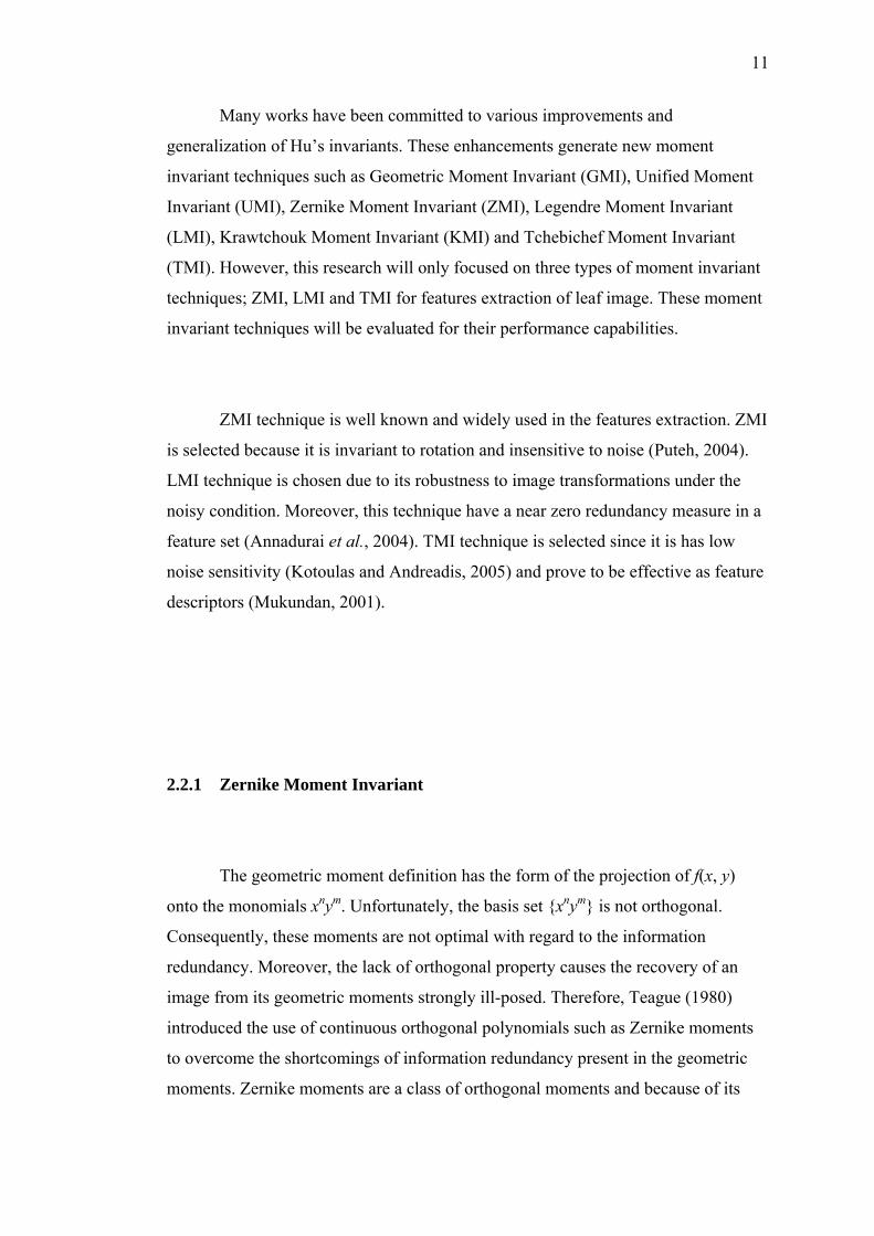
From the equation (2.2) it can be seen that Zernike moments use polynomials

of the image radius instead of monomials of Cartesian coordinates and a complex

exponential factor of the angle . This makes their complex modulus invariant to

rotation. Their orthogonal property renders image reconstruction from its moments

feasible and accurate. Furthermore, numerical instabilities are rare in compare to

13

geometric moments (Kotoulas and Andreadis, 2005). There are several advantages of

Zernike moments such as:

• The magnitudes of Zernike moments are invariant to rotation.

• Zernike moments are robust to noise and minor variations in shape

(Khotanzad, 1998).

• Zernike moments have minimum information redundancy since the

basis is orthogonal (Teague, 1980).

Nevertheless, the computation of Zernike moments poses some problems

such as (Mukundan et al., 2001):

• The coordinates of the image must be mapped to unit circle.

• Computational complexity of radial Zernike polynomial increase as

the order becomes larger.

2.2.2 Legendre Moment Invariant

The moments with Legendre polynomials as kernel function denoted as

Legendre moments were introduced by Teague (1980). Legendre Moment Invariants

(LMI) belongs to the class of orthogonal moments and they were used in several

pattern recognition applications. They can be used to attain a near zero value of

redundancy measure in a set of moments correspond to independent characteristics

of the image.

14

p q

i=0 j=0

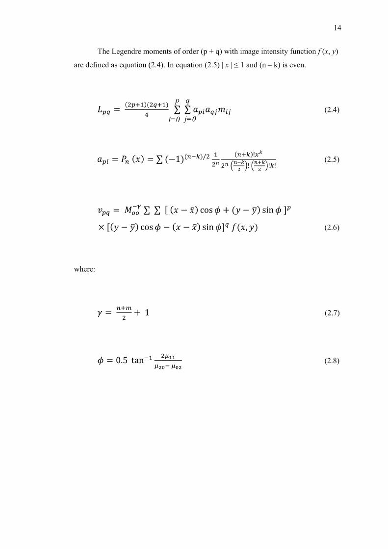
The Legendre moments of order (p + q) with image intensity function f (x, y)

are defined as equation (2.4). In equation (2.5) | x | ≤ 1 and (n – k) is even.

∑ ∑ (2.4)

∑ 1 / !

! ! ! (2.5)

∑ ∑ cos sin

cos sin , (2.6)

where:

1 (2.7)

0.5 tan

(2.8)

15

~

N-1

x=0

~

~

~

~ p

k=0

~

2.2.3 Tchebichef Moment Invariant

One common problem with the continuous moments is the discrete error,

which accumulates as the order of the moments increases (Yap et al., 2003).

Mukundan et al. (2001) introduced a set of discrete orthogonal moments function

based on the discrete Tchebichef polynomials to face this problem. The discrete

orthogonal polynomials is used as basis functions for image moments to eliminates

the need for numerical approximations and satisfies the orthogonal property in the

discrete domain of image coordinate space (Kotoulas and Andreadis, 2005).

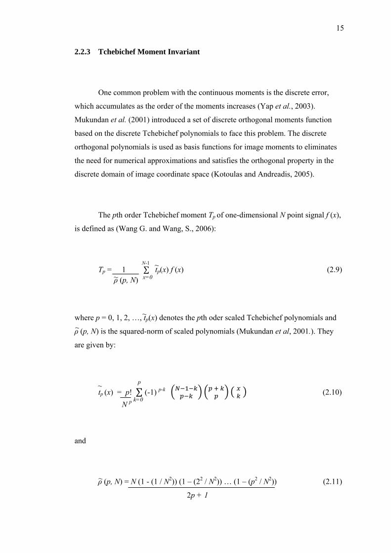
The pth order Tchebichef moment Tp of one-dimensional N point signal f (x),

is defined as (Wang G. and Wang, S., 2006):

Tp = 1 ∑ tp(x) f (x) (2.9) ρ (p, N)

where p = 0, 1, 2, …, tp(x) denotes the pth oder scaled Tchebichef polynomials and

ρ (p, N) is the squared-norm of scaled polynomials (Mukundan et al, 2001.). They

are given by:

tp (x) = p! ∑ (-1) p-k (2.10) N p

and

ρ (p, N) = N (1 - (1 / N2)) (1 – (22 / N2)) … (1 – (p2 / N2)) (2.11)

2p + 1

16

~ ~ ~ ~

x=0

N-1 M-1

y=0

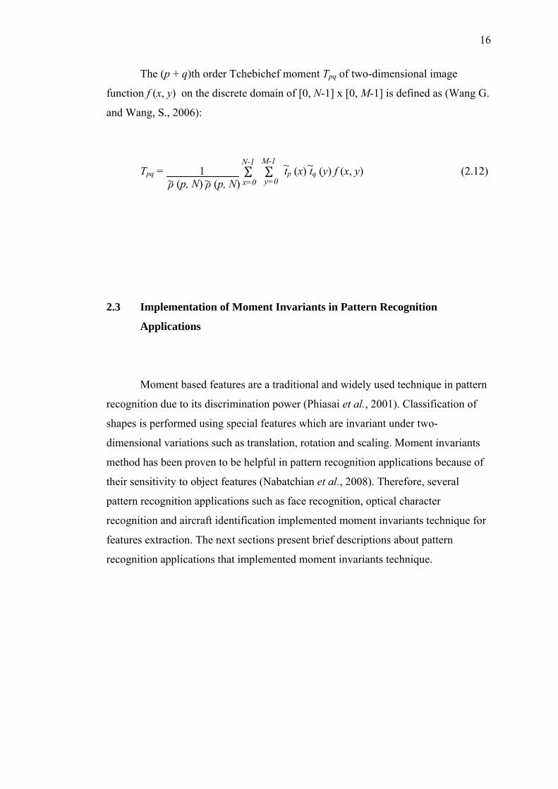
The (p + q)th order Tchebichef moment Tpq of two-dimensional image

function f (x, y) on the discrete domain of [0, N-1] x [0, M-1] is defined as (Wang G.

and Wang, S., 2006):

Tpq = 1 ∑ ∑ tp (x) tq (y) f (x, y) (2.12) ρ (p, N) ρ (p, N)

2.3 Implementation of Moment Invariants in Pattern Recognition

Applications

Moment based features are a traditional and widely used technique in pattern

recognition due to its discrimination power (Phiasai et al., 2001). Classification of

shapes is performed using special features which are invariant under two-

dimensional variations such as translation, rotation and scaling. Moment invariants

method has been proven to be helpful in pattern recognition applications because of

their sensitivity to object features (Nabatchian et al., 2008). Therefore, several

pattern recognition applications such as face recognition, optical character

recognition and aircraft identification implemented moment invariants technique for

features extraction. The next sections present brief descriptions about pattern

recognition applications that implemented moment invariants technique.

17

2.3.1 Face Recognition

Lately, the face recognition has been used more frequently for human

recognition and human authentication. It has been one of the popular topics in the

area of pattern recognition because of its applications in commercial and security

applications. Nowadays, the current technologies have made this application possible

for driver’s license, passport, national ID verification or security access.

Extraction of applicable features from the human face images is a crucial part

of the recognition. Thus, when designing a face recognition system with high

recognition rate, it is important to choose the proper feature extractor. Different

moment invariants have been used to extract features from human face images for

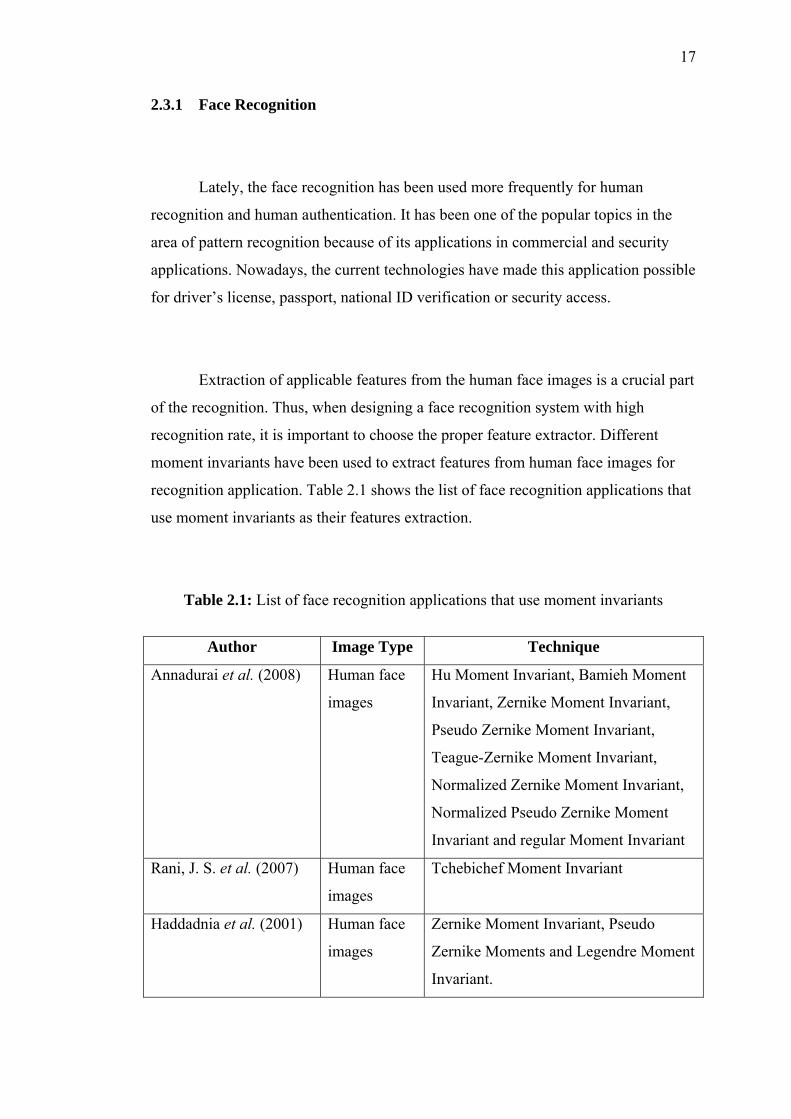
recognition application. Table 2.1 shows the list of face recognition applications that

use moment invariants as their features extraction.

Table 2.1: List of face recognition applications that use moment invariants

Author Image Type Technique

Annadurai et al. (2008) Human face

images

Hu Moment Invariant, Bamieh Moment

Invariant, Zernike Moment Invariant,

Pseudo Zernike Moment Invariant,

Teague-Zernike Moment Invariant,

Normalized Zernike Moment Invariant,

Normalized Pseudo Zernike Moment

Invariant and regular Moment Invariant

Rani, J. S. et al. (2007) Human face

images

Tchebichef Moment Invariant

Haddadnia et al. (2001) Human face

images

Zernike Moment Invariant, Pseudo

Zernike Moments and Legendre Moment

Invariant.

18

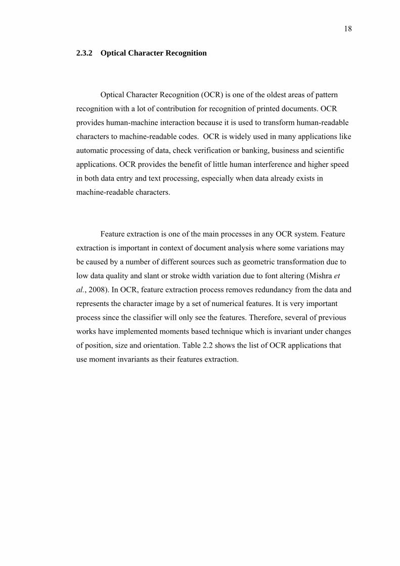
2.3.2 Optical Character Recognition

Optical Character Recognition (OCR) is one of the oldest areas of pattern

recognition with a lot of contribution for recognition of printed documents. OCR

provides human-machine interaction because it is used to transform human-readable

characters to machine-readable codes. OCR is widely used in many applications like

automatic processing of data, check verification or banking, business and scientific

applications. OCR provides the benefit of little human interference and higher speed

in both data entry and text processing, especially when data already exists in

machine-readable characters.

Feature extraction is one of the main processes in any OCR system. Feature

extraction is important in context of document analysis where some variations may

be caused by a number of different sources such as geometric transformation due to

low data quality and slant or stroke width variation due to font altering (Mishra et

al., 2008). In OCR, feature extraction process removes redundancy from the data and

represents the character image by a set of numerical features. It is very important

process since the classifier will only see the features. Therefore, several of previous

works have implemented moments based technique which is invariant under changes

of position, size and orientation. Table 2.2 shows the list of OCR applications that

use moment invariants as their features extraction.

19

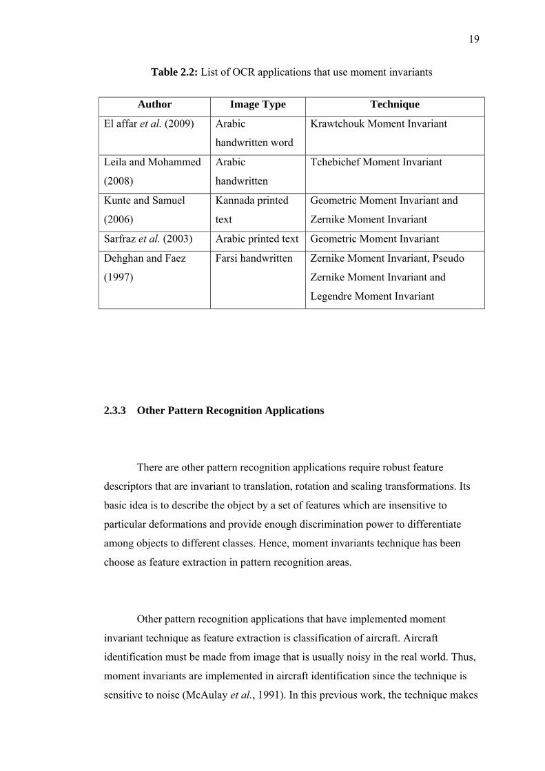
Table 2.2: List of OCR applications that use moment invariants

Author Image Type Technique

El affar et al. (2009) Arabic

handwritten word

Krawtchouk Moment Invariant

Leila and Mohammed

(2008)

Arabic

handwritten

Tchebichef Moment Invariant

Kunte and Samuel

(2006)

Kannada printed

text

Geometric Moment Invariant and

Zernike Moment Invariant

Sarfraz et al. (2003) Arabic printed text Geometric Moment Invariant

Dehghan and Faez

(1997)

Farsi handwritten Zernike Moment Invariant, Pseudo

Zernike Moment Invariant and

Legendre Moment Invariant

2.3.3 Other Pattern Recognition Applications

There are other pattern recognition applications require robust feature

descriptors that are invariant to translation, rotation and scaling transformations. Its

basic idea is to describe the object by a set of features which are insensitive to

particular deformations and provide enough discrimination power to differentiate

among objects to different classes. Hence, moment invariants technique has been

choose as feature extraction in pattern recognition areas.

Other pattern recognition applications that have implemented moment

invariant technique as feature extraction is classification of aircraft. Aircraft

identification must be made from image that is usually noisy in the real world. Thus,

moment invariants are implemented in aircraft identification since the technique is

sensitive to noise (McAulay et al., 1991). In this previous work, the technique makes

20

classification of aircraft robust in the presence of noise and some measure of scale,

translation and rotation invariance (McAulay et al., 1991). The moment invariants

provide the invariance and reduce the amount of data.

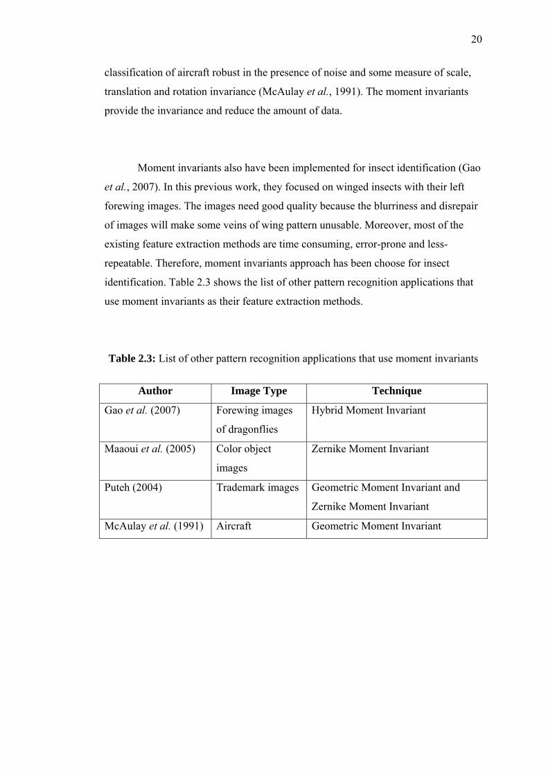
Moment invariants also have been implemented for insect identification (Gao

et al., 2007). In this previous work, they focused on winged insects with their left

forewing images. The images need good quality because the blurriness and disrepair

of images will make some veins of wing pattern unusable. Moreover, most of the

existing feature extraction methods are time consuming, error-prone and less-

repeatable. Therefore, moment invariants approach has been choose for insect

identification. Table 2.3 shows the list of other pattern recognition applications that

use moment invariants as their feature extraction methods.

Table 2.3: List of other pattern recognition applications that use moment invariants

Author Image Type Technique

Gao et al. (2007) Forewing images

of dragonflies

Hybrid Moment Invariant

Maaoui et al. (2005) Color object

images

Zernike Moment Invariant

Puteh (2004) Trademark images Geometric Moment Invariant and

Zernike Moment Invariant

McAulay et al. (1991) Aircraft Geometric Moment Invariant

21

2.4 Artificial Neural Networks

An Artificial Neural Network (ANN) is usually described as a network

composed of a large number of simple neurons that are massively interconnected,

operate in parallel and learn from experience. ANN was inspired by biological

findings involving the behavior of the brain as a network of units called neurons.

ANN is much simplified and bears only resemblance on the surface even though it is

modeled after biological neurons. Some of the major attributes of ANN such as they

can learn from examples, generalize well on unseen data and able to deal with

situation where the input data are incomplete or fuzzy (Kamruzzaman et al., 2006).

There have been hundreds of different models considered as ANNs since the

first neural model been introduced by McCulloch and Pitts (1943) that includes

General Regression Neural Network, which will be briefly discuss in the next

section. The differences in those models might be the functions, the accepted value,

the topology and learning algorithm. There are also many hybrid models where each

neuron has more properties. Neural networks have the ability to recognize patterns,

even when the information consist of these patterns is noisy or incomplete. Previous

works show that neural networks are very good pattern recognizers since they have

the ability to learn and build unique structures for a particular problem (Uhrig,

1995).

2.4.1 General Regression Neural Networks

General Regression Neural Network (GRNN) is proposed by Donald F.

Specht (1991) and it is belongs to the class of supervised networks. The GRNN is

based on radial basis function and operates in a similar way to PNN but perform

22

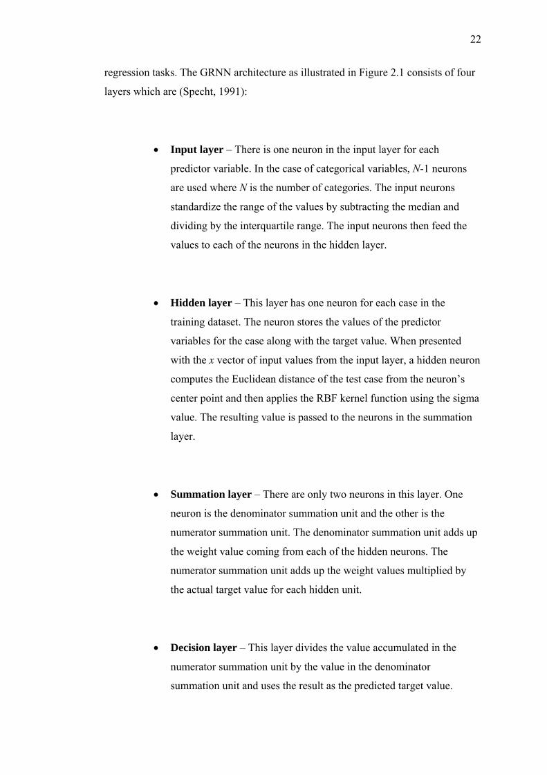
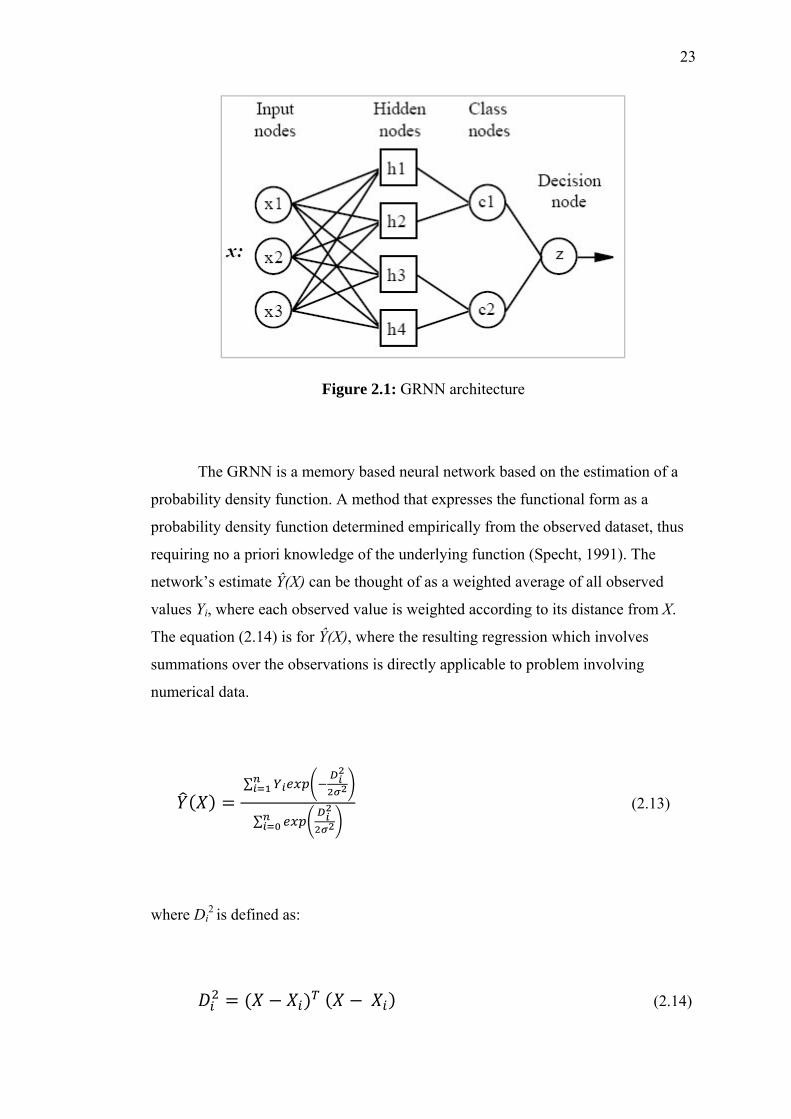
regression tasks. The GRNN architecture as illustrated in Figure 2.1 consists of four

layers which are (Specht, 1991):

• Input layer – There is one neuron in the input layer for each

predictor variable. In the case of categorical variables, N-1 neurons

are used where N is the number of categories. The input neurons

standardize the range of the values by subtracting the median and

dividing by the interquartile range. The input neurons then feed the

values to each of the neurons in the hidden layer.

• Hidden layer – This layer has one neuron for each case in the

training dataset. The neuron stores the values of the predictor

variables for the case along with the target value. When presented

with the x vector of input values from the input layer, a hidden neuron

computes the Euclidean distance of the test case from the neuron’s

center point and then applies the RBF kernel function using the sigma

value. The resulting value is passed to the neurons in the summation

layer.

• Summation layer – There are only two neurons in this layer. One

neuron is the denominator summation unit and the other is the

numerator summation unit. The denominator summation unit adds up

the weight value coming from each of the hidden neurons. The

numerator summation unit adds up the weight values multiplied by

the actual target value for each hidden unit.

• Decision layer – This layer divides the value accumulated in the

numerator summation unit by the value in the denominator

summation unit and uses the result as the predicted target value.

23

Figure 2.1: GRNN architecture

The GRNN is a memory based neural network based on the estimation of a

probability density function. A method that expresses the functional form as a

probability density function determined empirically from the observed dataset, thus

requiring no a priori knowledge of the underlying function (Specht, 1991). The

network’s estimate Ŷ(X) can be thought of as a weighted average of all observed

values Yi, where each observed value is weighted according to its distance from X.

The equation (2.14) is for Ŷ(X), where the resulting regression which involves

summations over the observations is directly applicable to problem involving

numerical data.

∑

∑ (2.13)

where Di2 is defined as:

(2.14)

24

The GRNN provides estimates of continuous variables and converges to the

underlying regression surface. This neural network is one pass learning algorithm

with highly parallel structure. The main advantages of GRNN are fast learning and

convergence to the optimal regression surface as the number of samples becomes

very large (Erkmen et al., 2006). GRNN approximates any arbitrary function

between input and output vectors, drawing the function estimate directly from the

training data. Moreover, it is consistent as the training set size becomes large, the

estimation error approaches zero, with only mild restrictions on the function (Avci,

2002).

2.5 Neural Networks Implementation

The interest in neural networks comes from the networks’ ability to imitate

human brain as well as its ability to learn and respond. As a result, neural networks

have been used in a large number of applications and have proven to be effective in

performing complex functions in a variety of fields. These include pattern

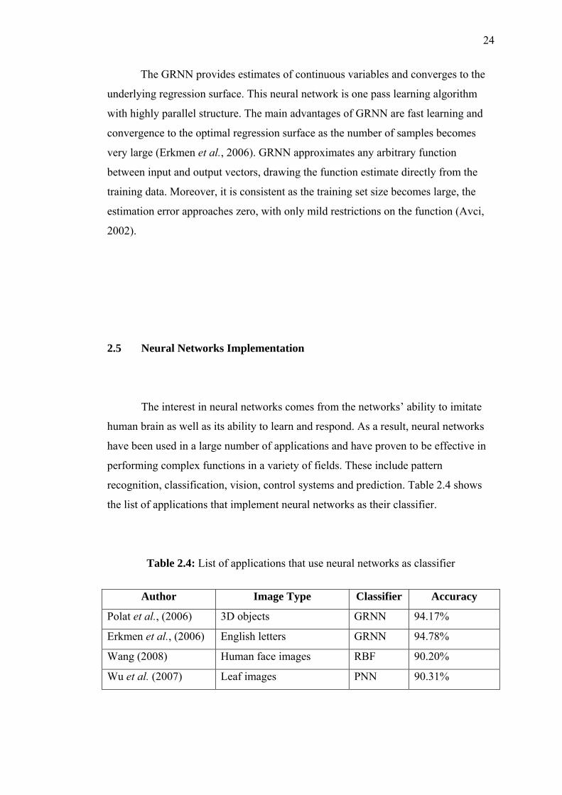
recognition, classification, vision, control systems and prediction. Table 2.4 shows

the list of applications that implement neural networks as their classifier.

Table 2.4: List of applications that use neural networks as classifier

Author Image Type Classifier Accuracy

Polat et al., (2006) 3D objects GRNN 94.17%

Erkmen et al., (2006) English letters GRNN 94.78%

Wang (2008) Human face images RBF 90.20%

Wu et al. (2007) Leaf images PNN 90.31%

25

Unlike multilayer feed-forward neural network which requires a large

number of iterations in training to converge to a desired solution, GRNN need only a

single pass of learning to achieve optimal performance in classification (Bhatti et al.,

2004). The GRNN is a powerful regression tool with a dynamic network structure

whose network training speed is extremely fast (Polat et al., 2006). Due to the

simplicity of the network structure and its implementation, it has been widely

applied to a variety of fields. Therefore, the GRNN is chosen as classifier for plant

leaf identification.

2.6 Summary

This chapter explains about the domain of the research which is leaf features

extraction and classification. It gives some briefing of feature extraction which

involves the leaf extraction by features that are suitable for classification and have at

least translation, scale and rotation invariance. Several feature extraction methods

have been discussed in this chapter such as ZMI, LMI and TMI. These methods have

been implemented in various pattern recognition applications that include face

recognition, optical character recognition and aircraft identification as their feature

extraction. Therefore, these methods have been chosen to be implementing in the

plant leaf identification and the comparison of their performances will be make. This

chapter also described the neural networks as classifier for classification of plant

leaf. A brief discussion about GRNN is made and it shows that this neural networks

offer better features for recognition applications. In addition, it gives high efficient

training. Thus, for the plant leaf identification, GRNN is chosen to be implementing

as classifier for this research.

CHAPTER 3

METHODOLOGY

3.1 Introduction

At each operational step in the research process, researchers are required to

choose from multiplicity of methods, procedures and models of research

methodology which will help them to best achieve research objectives. The research

techniques, procedures and methods that form the body of research methodology are

applied to the collection of information about various aspects of a situation, issue or

problem so that the information gathered can be used in other ways. This is where

research methodology plays crucial role. Therefore, this chapter will explain the

major activities involved in this project in order to achieve the objectives and solve

the background problems. In addition, the research operational framework, software

and equipments requirements also will be discussed.

27

3.2 Research Framework

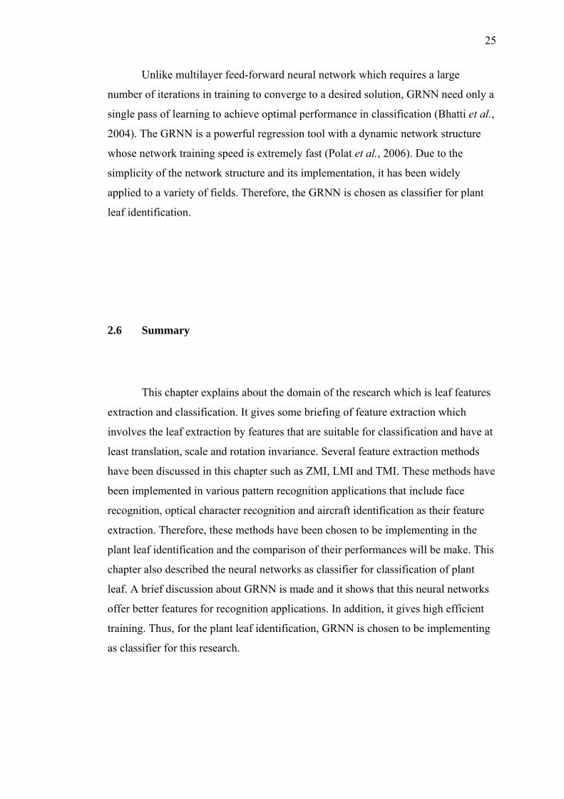
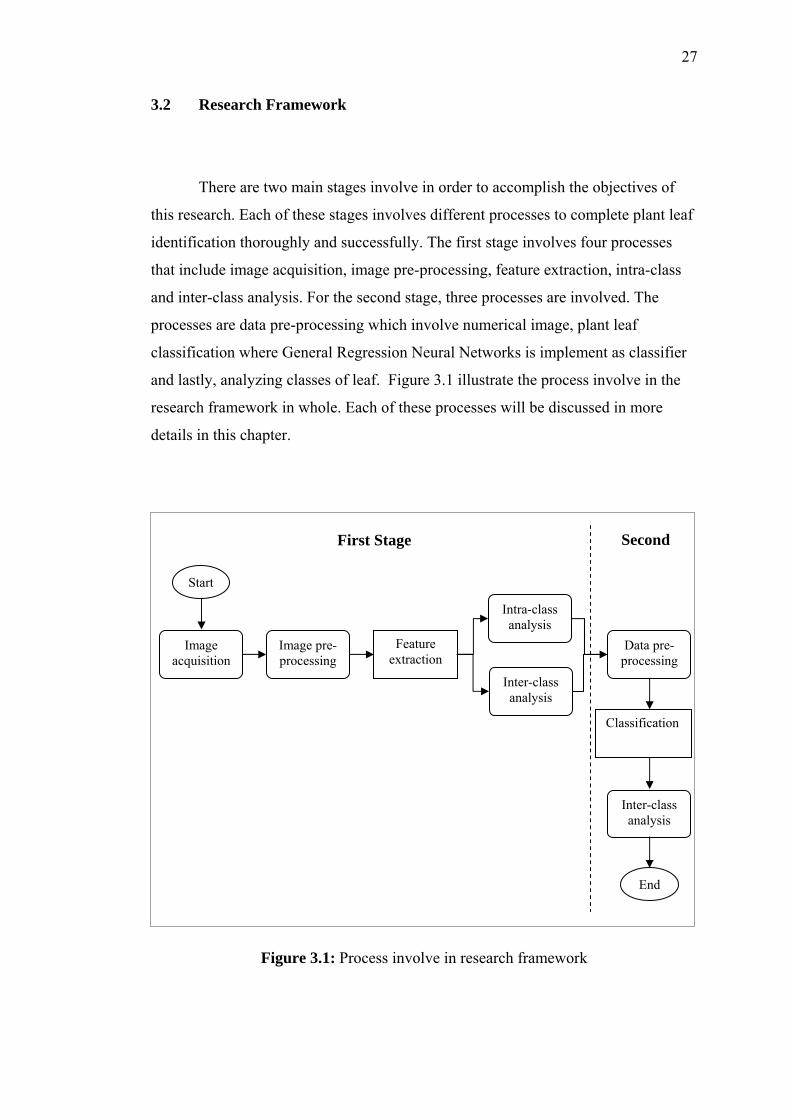
There are two main stages involve in order to accomplish the objectives of

this research. Each of these stages involves different processes to complete plant leaf

identification thoroughly and successfully. The first stage involves four processes

that include image acquisition, image pre-processing, feature extraction, intra-class

and inter-class analysis. For the second stage, three processes are involved. The

processes are data pre-processing which involve numerical image, plant leaf

classification where General Regression Neural Networks is implement as classifier

and lastly, analyzing classes of leaf. Figure 3.1 illustrate the process involve in the

research framework in whole. Each of these processes will be discussed in more

details in this chapter.

Figure 3.1: Process involve in research framework

First Stage Second

Feature extraction

Image acquisition

Start

Image pre-processing

Intra-class analysis

Inter-class analysis

Data pre-processing

Classification

End

Inter-class analysis

28

3.3 Software Requirement

The software requirement during feature extraction phase of this research

includes Borland C++ 5.02. A moment invariants algorithm is build using C

programming languages. Therefore, this software is used since it can handle the C

programming language. Moreover, it can run the moment invariants algorithm more

effectively. For classification phase, the software used is MATLAB 7.8. This

software provides Neural Network Toolbox which makes it easier to use neural

networks in MATLAB. The toolbox consists of a set of functions and structures that

can handle neural networks for classification task.

3.4 Image Source

The implementation of feature extraction methods and classifier will be tested

and evaluated using plant leaf images. The collection of leaf images are from variety

of plants. The procedure is that the leaf from plant is pluck and then, the digital color

image of the leaf is taken with a digital camera. When taken the leaf photo, there is

no restriction on the direction of leaves. In this research, 10 species of different

plants will be use. Each species includes 10 samples of leaf images. These leaf

images come in with different of size, shapes and class.

29

3.5 Image Pre-processing

Image pre-processing does not increase the image information content. It is

useful on a variety of situations where it helps to suppress information that is not

relevant to the specific image processing or analysis task. The aim of image pre-

processing is to improve image data so that it can suppress undesired distortions and

enhances the image features that are relevant for further processing.

Pre-processing of leaf images prior to plant leaf identification is essential.

The main purpose of this process is to provide images that follow fixed scaling and

rotation factors. These images will become an input to feature extraction phase. The

images with its various rotations and scaling factor are evaluated with feature

extraction methods to examine their invariant characteristics.

Pre-processing usually contains a series of sequential operations including

prescribe the image size, conversion of gray-scale images to binary images

(monochrome) file and modify the scaling and rotation factors of the image. Brief

descriptions of the images pre-processing steps for this research are as follows:

a) The images are minimized to 210 x 314 pixel dimensions in order to

ease the computational burden.

b) In order to use pixels with values of 0 and 1, the grey-scale images are

converted to binary images. The binary images are often produced by

thresholding a grays-scale or color image, in order to separate an

object in the image from the background. Each image has its own

threshold value; therefore the value is not fixed. Then, the image is

saved using the .raw format.

30

c) Each leaf images have 12 variant images with different scaling and

rotation factors. For image scaling factor, four values are used and for

image rotation factor, four degree values are used. The remaining four

images are influenced by combination of scaling and rotation factors.

Table 3.1 illustrates the value of scaling and rotation factors. This

research used 120 binary images that represent 10 different plant

leaves.

Table 3.1: The value of scaling and rotation factors

No. Geometric Transformations Factors

1 The image is reduced to 0.5x

2 The image is reduced to 0.75x

3 The image is enlarged to 1.2x

4 The image is enlarged to 1.4x

5 The image is rotated to 10°

6 The image is rotated to 20°

7 The image is rotated to 45°

8 The image is rotated to 90°

9 The image is reduced to 0.5x and rotated to 10°

10 The image is reduced to 0.75x and rotated to 20°

11 The image is enlarged to 1.2x and rotated to 45°

12 The image is enlarged to 1.4x and rotated to 90°

3.6 Feature Extraction

The next stage in the plant leaf identification is the feature extraction phase.

The main advantage of this phase is that it removes redundancy from the image and

31

represents the leaf image by a set of numerical features. These features are used by

the classifier to classify the data. In this research, moment invariants have been used

to build up the feature space. This technique has the desirable property of being

invariant under image scaling, rotation and translation.

The moment-based feature extraction technique is performed in order to

extract the global image shape of binary image. This technique performed well in

extracting the global image shape (Puteh and Norsalasawati, 2004). In this research,

three types of moment invariant techniques are used to generate features vector of

leaf images; namely ZMI, LMI and TMI. These features vector are analyzed to

examine their invariant characteristics.

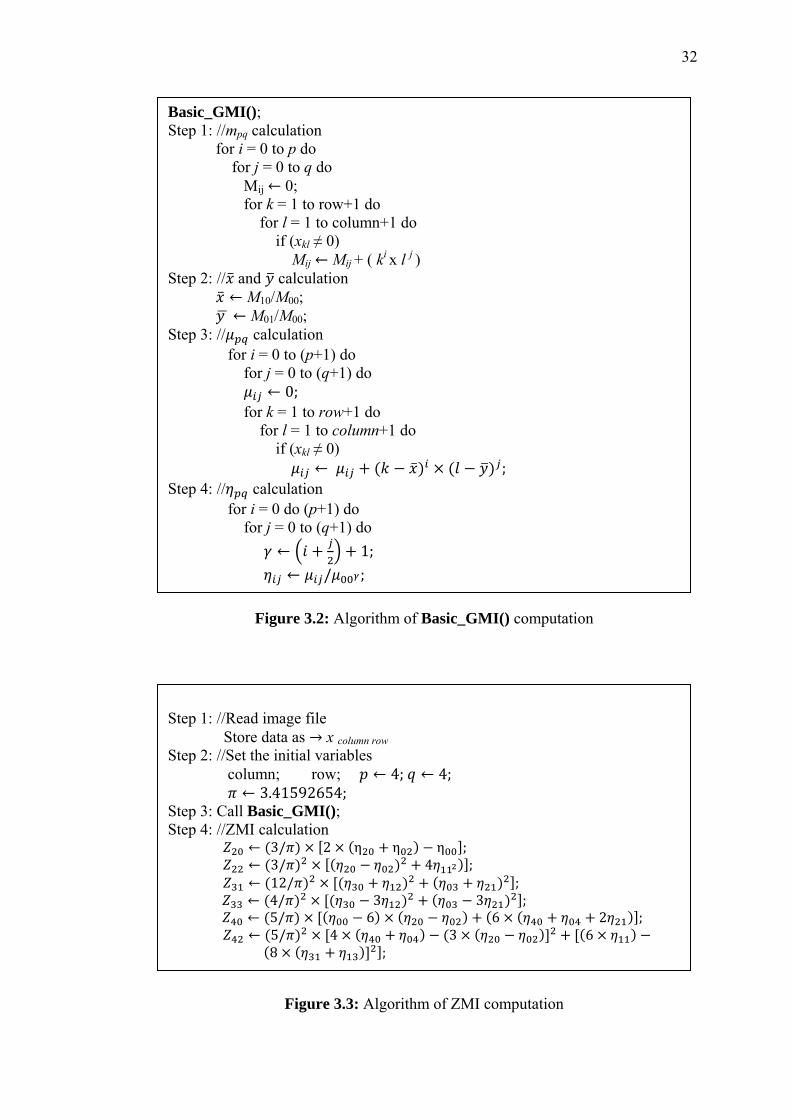
3.6.1 ZMI Algorithm

ZMI algorithm has quite complex calculation and Figure 3.2 shows the

algorithm of ZMI computation. The GMI technique is the basic technique to others

moments technique and this technique is focused on Basic_GMI() function as shown

in Figure 3.3. Zernike’s rule can be reputedly connected with geometric moments

until third order in Step 4. The existing Zernike translation invariants can be

indirectly obtained by making use of the existing geometric central moments.

Normalized central moment, computation is used in image scaling.

32

Figure 3.2: Algorithm of Basic_GMI() computation

Figure 3.3: Algorithm of ZMI computation

Basic_GMI(); Step 1: //mpq calculation for i = 0 to p do for j = 0 to q do Mij 0; for k = 1 to row+1 do for l = 1 to column+1 do if (xkl ≠ 0) Mij Mij + ( ki x l j ) Step 2: // and calculation M10/M00; M01/M00; Step 3: // calculation for i = 0 to (p+1) do for j = 0 to (q+1) do 0; for k = 1 to row+1 do for l = 1 to column+1 do if (xkl ≠ 0) ; Step 4: // calculation for i = 0 do (p+1) do for j = 0 to (q+1) do 1; / ;

Step 1: //Read image file Store data as x column row Step 2: //Set the initial variables column; row; 4; 4; 3.41592654; Step 3: Call Basic_GMI(); Step 4: //ZMI calculation 3/ 2 η η η ; 3/ 4 ; 12/ ; 4/ 3 3 ; 5/ 6 6 2 ; 5/ 4 3 6 8 ;

33

Step 1: // calculation 0.5 tan 2 / ; Step 2: // calculation for i = 0 to p do for j = 0 to q do /2 1; 0; for k = 1 to row+1 do for l = 1 to column+1 do if (xkl ≠ 0) cos sin

1/ ;

cos sin ;

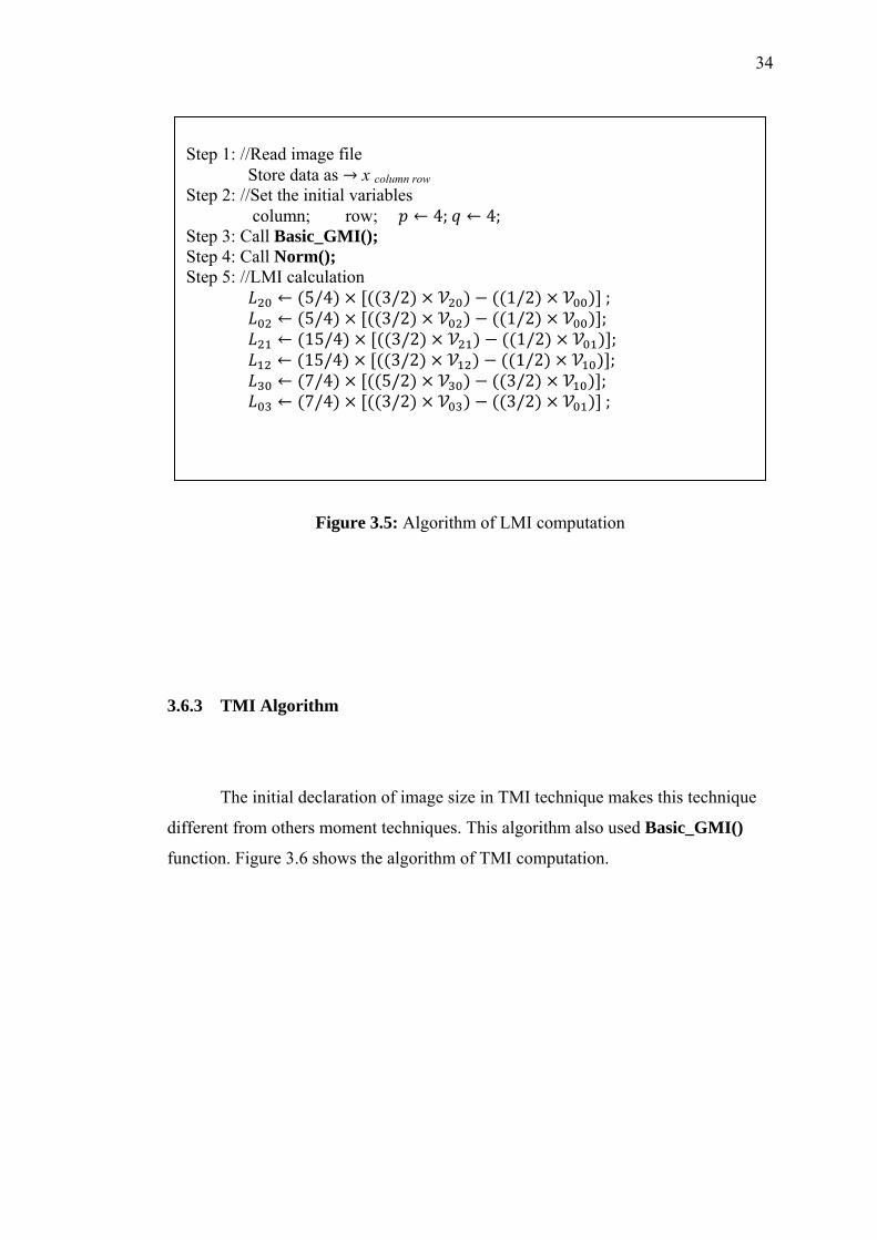
3.6.2 LMI Algorithm

A new computation function, Norm() as shown in Figure 3.4 is introduced in

LMI technique. Legendre moments computation does not have invariants

characteristics. Therefore, Norm() is used to overcome this disadvantage because the

function provide invariants characteristics to rotation, translation and scaling factors.

However, Basic_GMI() function need to be called first in order to obtain the value

of , and for Norm() function in Step 1. Figure 3.5 illustrates the algorithm

of LMI computation.

Figure 3.4: Algorithm of Norm() computation

34

Figure 3.5: Algorithm of LMI computation

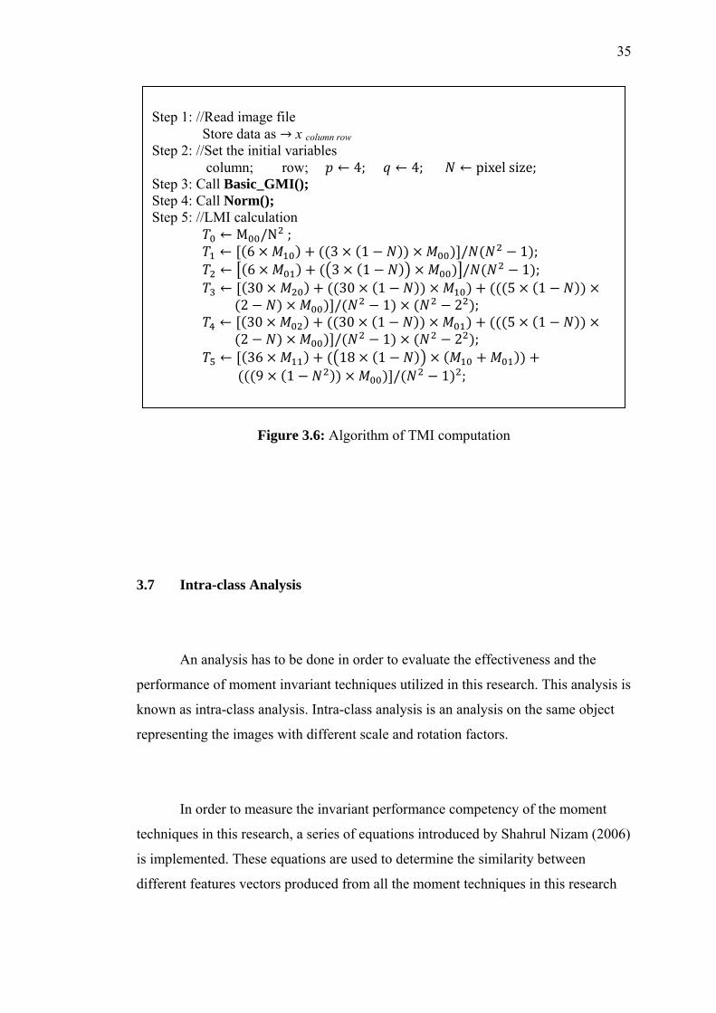
3.6.3 TMI Algorithm

The initial declaration of image size in TMI technique makes this technique

different from others moment techniques. This algorithm also used Basic_GMI()

function. Figure 3.6 shows the algorithm of TMI computation.

Step 1: //Read image file Store data as x column row Step 2: //Set the initial variables column; row; 4; 4; Step 3: Call Basic_GMI(); Step 4: Call Norm(); Step 5: //LMI calculation 5/4 3/2 1/2 ; 5/4 3/2 1/2 ; 15/4 3/2 1/2 ; 15/4 3/2 1/2 ; 7/4 5/2 3/2 ; 7/4 3/2 3/2 ;

35

Figure 3.6: Algorithm of TMI computation

3.7 Intra-class Analysis

An analysis has to be done in order to evaluate the effectiveness and the

performance of moment invariant techniques utilized in this research. This analysis is

known as intra-class analysis. Intra-class analysis is an analysis on the same object

representing the images with different scale and rotation factors.

In order to measure the invariant performance competency of the moment

techniques in this research, a series of equations introduced by Shahrul Nizam (2006)

is implemented. These equations are used to determine the similarity between

different features vectors produced from all the moment techniques in this research

2 / 1 2 ;

2 / 1 2 ;

9 1 / 1 ;

Step 1: //Read image file Store data as x column row Step 2: //Set the initial variables column; row; 4; 4; pixel size; Step 3: Call Basic_GMI(); Step 4: Call Norm(); Step 5: //LMI calculation M /N ; 6 3 1 / 1 ; 6 3 1 / 1 ; 30 30 1 5 1

30 30 1 5 1

36 18 1

36

that represent the same object of the particular image. These equations are known as

Invariant Error Computation (IEC). The features vector for original image is give by:

Ha ( γi ) = { γi , γi + 1 , γi + 2 , … , γn } (3.1)

where a is referred as the class name with i is the feature dimension. Each class

consists of a set of images generated by transforming the original image with

different scale and orientations. Therefore, each features vector for the variations of

images is given by:

( γi ) = { γi , γi + 1 , γi + 2 , … , γn } (3.2)

where m refers to the type of variations of class a. Therefore, there will be several

feature vectors representing the images with different scale and orientations for one

object.

To calculate the absolute error for each dimension, equations (3.3) is used. In

order to make comparison of each pattern of class a, the percentage of absolute error

of each pattern is perform using equation (3.4). Equation (3.5) is computed to obtain

the percentage of mean absolute error for the feature vector for the variations of

class. In order to examine an error distribution along the dimension of each features

vectors are illustrate in equation (3.6). Lastly, equation (3.7) and (3.8) is utilized to

calculate the total error of class a for each moment invariant method.

∆ | | (3.3)

37

I

i = 1

M

m = 1

M

m = 1

i = 1

n

%∆ ∆ | |

100 (3.4)

1 ∑ (3.5)

2 ∑ (3.6)

∑ 1 (3.7)

∑ 2 (3.8)

3.8 Inter-class Analysis

Inter-class analysis is conducted by making a comparison between values of

feature vectors based on the original image used in this research. Different moment

invariant methods will generate a different value of feature vectors for the same

image. Hence, each group of data produced by different technique definitely has its

own feature space. In order to analyze the different value of feature vectors for the

images, each feature vectors value of the original image is put into a table according

to the moment invariant methods used. The comparison is examined based on the

characteristic of feature vectors value, the similarity and dissimilarity of those values.

Other than that, computational time for each moment invariants methods to extract

38

feature vectors is taken. The purpose is to examine which methods have fast

computational speed so that it can be implemented later.

3.9 Data Pre-processing

Data pre-processing describes any type of processing performed on raw data

to prepare it for another processing procedure. The main purpose of the data pre-

processing stage is to manipulate the raw data into a form with which a neural

network can be trained. The data pre-processing can often have a significant impact

on the performance of a neural network. Therefore, before applying any of the built-

in functions for training, it is important to check that the data is reasonable.

Before this process is performed, the data obtained from the feature

extraction methods are in a numeric form or measures. Thus, in order to obtain an

effective training of neural networks, the numeric data should be scaled. This process

is known as normalization. Normalization is a scaling down transformation of the

features. There is often a large difference between the maximum and minimum

values within a feature. When normalization is performed, magnitudes of the values

is normalized and scaled to appreciably low values. This is important for many

neural network algorithms. One form of suitable data normalization can be achieved

using equation (3.9) which is known as Linear Transformation equation. The scaled

variable should be within the range of 0 to 1.

(3.9)

39

(3.10)

where:

v’ is the new feature value that been normalized.

vo is the old feature value before normalized.

vmin is minimum feature value in the data sample.

vmax is maximum feature value in the data sample.

3.10 Classification by Neural Networks

In this research, a GRNN is utilized as classifier in plant leaf identification.

This network is trained in supervised manner. Therefore, the input data is normalized

so that the feature vectors values is in the range of 0 to 1. Otherwise, normalization

process is ignored if the feature vectors values obtained is in that range.

The dataset is divided into training dataset, validation dataset and testing

dataset. Training dataset is used for learning and to fit parameters of the classifier.

To evaluate the success of the network, validation dataset is used to test the

network’s ability to generalize the data and tune the parameters of classifier. After

fixed iterations have completely been carried out, the testing dataset is used in the

trained network in order to estimate the error rate so that the network can recognize

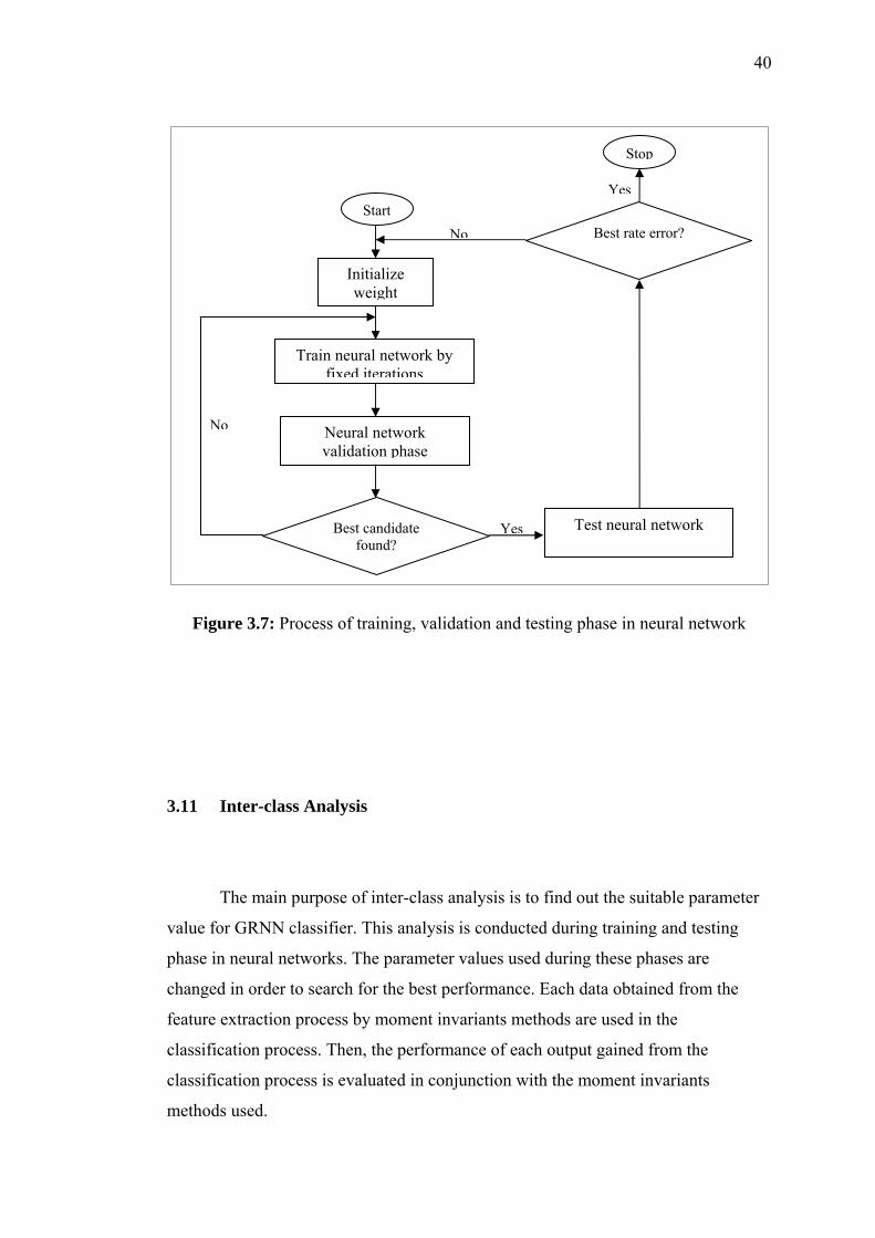
the pattern effectively. Figure 3.2 shows the process of training, validation and

testing phase in neural network.

40

Figure 3.7: Process of training, validation and testing phase in neural network

3.11 Inter-class Analysis

The main purpose of inter-class analysis is to find out the suitable parameter

value for GRNN classifier. This analysis is conducted during training and testing

phase in neural networks. The parameter values used during these phases are

changed in order to search for the best performance. Each data obtained from the

feature extraction process by moment invariants methods are used in the

classification process. Then, the performance of each output gained from the

classification process is evaluated in conjunction with the moment invariants

methods used.

Yes

No

No

YesStart

Initialize weight

Train neural network by fixed iterations

Neural network validation phase

Test neural network

Stop

Best candidate found?

Best rate error?

41

k

k=1

t=1

The method of k-fold cross validation is used to find the generalization

performance of GRNN classifier in combination with different types of features

extraction. The k-fold cross validation is one way to improve over the holdout

method. The dataset is divided into k subsets and the holdout method is repeated k

times. Each time, one of the k subsets is used as the test dataset and the other k – 1

subsets are put together to form the training dataset. Then, the average error cross all

k trials is computed. Every data point gets to be in a test exactly once and in training

set k – 1 times.

In this research, the dataset is split into k subsets. Then, the classifier is

trained and tested k-times. The cross validation estimate is identified as the number

of correct classification divided by the number of data points. The percentage of

correct classification (PCC) is given by the equation (3.11) and the number of correct

classification (NCC) is given by (3.12). If the testing vector is true, σ (x, y)t = 1.

Otherwise, σ (x, y)t = 0.

100 ∑ (3.11)

∑ , (3.12)

where n refers to the number of data tested.

n

42

3.12 Summary

As a conclusion, this chapter explains briefly on this research methodology

where it involves two main stages which include feature extraction phase and

classification phase. The processes involved in this research are presented in the

research framework. Each process implemented in this research is dependent with

one another. The next chapter will describes briefly about the initial finding of this

research.

CHAPTER 4

IMPLEMENTATION, COMPARISON OF RESULTS

AND DISCUSSION

4.1 Introduction

This chapter will discussed the implementation processes of this research.

These implementation processes involve two stages. The first stage involves several

processes that include image pre-processing, feature extraction of leaf images, intra-

class and inter-class analysis. Moment invariants methods such as ZMI, LMI and

TMI are applied in the feature extraction process. As for the second stage, the

processes involved are data pre-processing, classification of leaf images and inter-

class analysis. For classification process, GRNN is applied as the classifier. The

implementation methods and the results achieved will be describes briefly in this

chapter.

44

4.2 Leaf Images

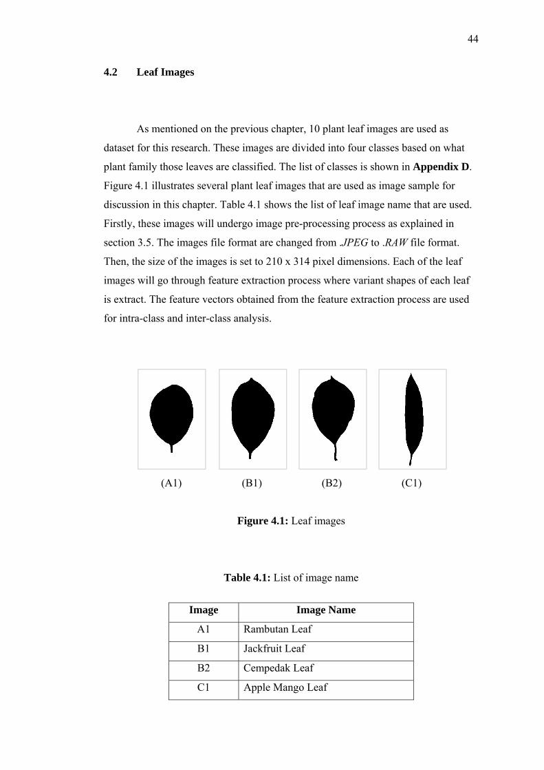
As mentioned on the previous chapter, 10 plant leaf images are used as

dataset for this research. These images are divided into four classes based on what

plant family those leaves are classified. The list of classes is shown in Appendix D.

Figure 4.1 illustrates several plant leaf images that are used as image sample for

discussion in this chapter. Table 4.1 shows the list of leaf image name that are used.

Firstly, these images will undergo image pre-processing process as explained in

section 3.5. The images file format are changed from .JPEG to .RAW file format.

Then, the size of the images is set to 210 x 314 pixel dimensions. Each of the leaf

images will go through feature extraction process where variant shapes of each leaf

is extract. The feature vectors obtained from the feature extraction process are used

for intra-class and inter-class analysis.

(A1) (B1) (B2) (C1)

Figure 4.1: Leaf images

Table 4.1: List of image name

Image Image Name

A1 Rambutan Leaf

B1 Jackfruit Leaf

B2 Cempedak Leaf

C1 Apple Mango Leaf

45

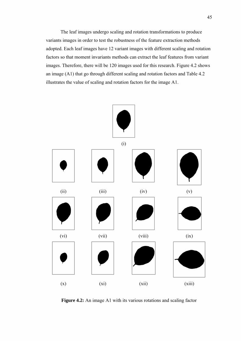
The leaf images undergo scaling and rotation transformations to produce

variants images in order to test the robustness of the feature extraction methods

adopted. Each leaf images have 12 variant images with different scaling and rotation

factors so that moment invariants methods can extract the leaf features from variant

images. Therefore, there will be 120 images used for this research. Figure 4.2 shows

an image (A1) that go through different scaling and rotation factors and Table 4.2

illustrates the value of scaling and rotation factors for the image A1.

(i)

(ii) (iii) (iv) (v)

(vi) (vii) (viii) (ix)

(x) (xi) (xii) (xiii)

Figure 4.2: An image A1 with its various rotations and scaling factor

46

Table 4.2: Scaling and rotation factors of image A1

Image Geometric Transformations Factors

(i) An original image

(ii) The image is reduced to 0.5x

(iii) The image is reduced to 0.75x

(iv) The image is enlarged to 1.2x

(v) The image is enlarged to 1.4x

(vi) The image is rotated to 10°

(vii) The image is rotated to 20°

(viii) The image is rotated to 45°

(ix) The image is rotated to 90°

(x) The image is reduced to 0.5x and rotated to 10°

(xi) The image is reduced to 0.75x and rotated to 20°

(xii) The image is enlarged to 1.2x and rotated to 45°

(xiii) The image is enlarged to 1.4x and rotated to 90°

4.3 Result of Intra-class Analysis

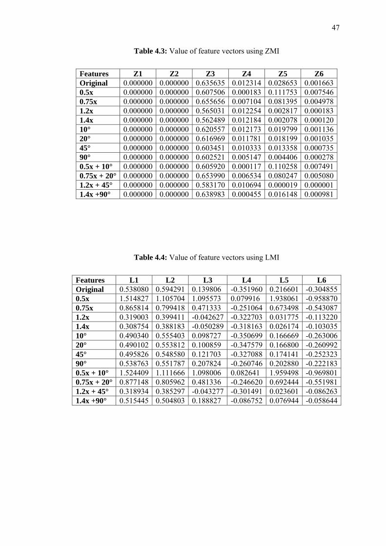
As mentioned in Chapter 3, intra-class analysis is an analysis on the same

object representing the images with different scale and rotation factors in order to

evaluate the effectiveness of three moment invariants used in this research. The ZMI,

LMI and TMI algorithm is used on the image A1 to generate value of feature

vectors. The value of feature vectors obtained is shown in Table 4.3, 4.4 and 4.5.

Based on all the tables, different moment technique will generate a different value of

feature vectors. Thus, each group of data produced by different techniques certainly

has its own feature space.

47

Table 4.3: Value of feature vectors using ZMI

Features Z1 Z2 Z3 Z4 Z5 Z6 Original 0.000000 0.000000 0.635635 0.012314 0.028653 0.0016630.5x 0.000000 0.000000 0.607506 0.000183 0.111753 0.0075460.75x 0.000000 0.000000 0.655656 0.007104 0.081395 0.0049781.2x 0.000000 0.000000 0.565031 0.012254 0.002817 0.0001831.4x 0.000000 0.000000 0.562489 0.012184 0.002078 0.00012010° 0.000000 0.000000 0.620557 0.012173 0.019799 0.00113620° 0.000000 0.000000 0.616969 0.011781 0.018199 0.00103545° 0.000000 0.000000 0.603451 0.010333 0.013358 0.00073590° 0.000000 0.000000 0.602521 0.005147 0.004406 0.0002780.5x + 10° 0.000000 0.000000 0.605920 0.000117 0.110258 0.0074910.75x + 20° 0.000000 0.000000 0.653990 0.006534 0.080247 0.0050801.2x + 45° 0.000000 0.000000 0.583170 0.010694 0.000019 0.0000011.4x +90° 0.000000 0.000000 0.638983 0.000455 0.016148 0.000981

Table 4.4: Value of feature vectors using LMI

Features L1 L2 L3 L4 L5 L6 Original 0.538080 0.594291 0.139806 -0.351960 0.216601 -0.3048550.5x 1.514827 1.105704 1.095573 0.079916 1.938061 -0.9588700.75x 0.865814 0.799418 0.471333 -0.251064 0.673498 -0.5430871.2x 0.319003 0.399411 -0.042627 -0.322703 0.031775 -0.1132201.4x 0.308754 0.388183 -0.050289 -0.318163 0.026174 -0.10303510° 0.490340 0.555403 0.098727 -0.350699 0.166669 -0.26300620° 0.490102 0.553812 0.100859 -0.347579 0.166800 -0.26099245° 0.495826 0.548580 0.121703 -0.327088 0.174141 -0.25232390° 0.538763 0.551787 0.207824 -0.260746 0.202880 -0.2221830.5x + 10° 1.524409 1.111666 1.098006 0.082641 1.959498 -0.9698010.75x + 20° 0.877148 0.805962 0.481336 -0.246620 0.692444 -0.5519811.2x + 45° 0.318934 0.385297 -0.043277 -0.301491 0.023601 -0.0862631.4x +90° 0.515445 0.504803 0.188827 -0.086752 0.076944 -0.058644

48

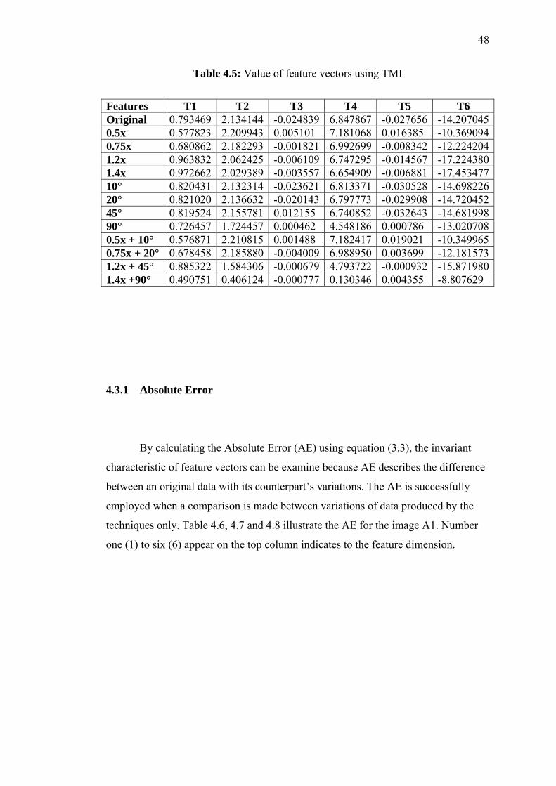
Table 4.5: Value of feature vectors using TMI

Features T1 T2 T3 T4 T5 T6 Original 0.793469 2.134144 -0.024839 6.847867 -0.027656 -14.2070450.5x 0.577823 2.209943 0.005101 7.181068 0.016385 -10.3690940.75x 0.680862 2.182293 -0.001821 6.992699 -0.008342 -12.2242041.2x 0.963832 2.062425 -0.006109 6.747295 -0.014567 -17.2243801.4x 0.972662 2.029389 -0.003557 6.654909 -0.006881 -17.45347710° 0.820431 2.132314 -0.023621 6.813371 -0.030528 -14.69822620° 0.821020 2.136632 -0.020143 6.797773 -0.029908 -14.72045245° 0.819524 2.155781 0.012155 6.740852 -0.032643 -14.68199890° 0.726457 1.724457 0.000462 4.548186 0.000786 -13.0207080.5x + 10° 0.576871 2.210815 0.001488 7.182417 0.019021 -10.3499650.75x + 20° 0.678458 2.185880 -0.004009 6.988950 0.003699 -12.1815731.2x + 45° 0.885322 1.584306 -0.000679 4.793722 -0.000932 -15.8719801.4x +90° 0.490751 0.406124 -0.000777 0.130346 0.004355 -8.807629

4.3.1 Absolute Error

By calculating the Absolute Error (AE) using equation (3.3), the invariant

characteristic of feature vectors can be examine because AE describes the difference

between an original data with its counterpart’s variations. The AE is successfully

employed when a comparison is made between variations of data produced by the

techniques only. Table 4.6, 4.7 and 4.8 illustrate the AE for the image A1. Number

one (1) to six (6) appear on the top column indicates to the feature dimension.

49

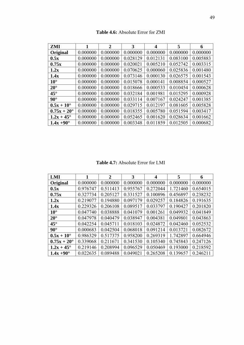
Table 4.6: Absolute Error for ZMI

ZMI 1 2 3 4 5 6 Original 0.000000 0.000000 0.000000 0.000000 0.000000 0.0000000.5x 0.000000 0.000000 0.028129 0.012131 0.083100 0.0058830.75x 0.000000 0.000000 0.020021 0.005210 0.052742 0.0033151.2x 0.000000 0.000000 0.070625 0.000060 0.025836 0.0014801.4x 0.000000 0.000000 0.073146 0.000130 0.026575 0.00154310° 0.000000 0.000000 0.015078 0.000141 0.008854 0.00052720° 0.000000 0.000000 0.018666 0.000533 0.010454 0.00062845° 0.000000 0.000000 0.032184 0.001981 0.015295 0.00092890° 0.000000 0.000000 0.033114 0.007167 0.024247 0.0013850.5x + 10° 0.000000 0.000000 0.029715 0.012197 0.081605 0.0058280.75x + 20° 0.000000 0.000000 0.018355 0.005780 0.051594 0.0034171.2x + 45° 0.000000 0.000000 0.052465 0.001620 0.028634 0.0016621.4x +90° 0.000000 0.000000 0.003348 0.011859 0.012505 0.000682

Table 4.7: Absolute Error for LMI

LMI 1 2 3 4 5 6 Original 0.000000 0.000000 0.000000 0.000000 0.000000 0.0000000.5x 0.976747 0.511413 0.955767 0.272044 1.721460 0.6540150.75x 0.327734 0.205127 0.331527 0.100896 0.456897 0.2382321.2x 0.219077 0.194880 0.097179 0.029257 0.184826 0.1916351.4x 0.229326 0.206108 0.089517 0.033797 0.190427 0.20182010° 0.047740 0.038888 0.041079 0.001261 0.049932 0.04184920° 0.047978 0.040479 0.038947 0.004381 0.049801 0.04386345° 0.042254 0.045711 0.018103 0.024872 0.042460 0.05253290° 0.000683 0.042504 0.068018 0.091214 0.013721 0.0826720.5x + 10° 0.986329 0.517375 0.958200 0.269319 1.742897 0.6649460.75x + 20° 0.339068 0.211671 0.341530 0.105340 0.745843 0.2471261.2x + 45° 0.219146 0.208994 0.096529 0.050469 0.193000 0.2185921.4x +90° 0.022635 0.089488 0.049021 0.265208 0.139657 0.246211

50

Table 4.8: Absolute Error for TMI

TMI 1 2 3 4 5 6 Original 0.000000 0.000000 0.000000 0.000000 0.000000 0.0000000.5x 0.215646 0.075799 0.019738 0.333201 0.011271 3.8379510.75x 0.112607 0.048149 0.023018 0.144832 0.019314 1.9828411.2x 0.170363 0.071719 0.081730 0.100572 0.013089 3.0173351.4x 0.179193 0.104755 0.021282 0.192958 0.020775 3.24643210° 0.026962 0.001830 0.001218 0.034496 0.002872 0.49118120° 0.027551 0.002488 0.004696 0.050094 0.002252 0.51340745° 0.026055 0.021637 0.012684 0.107015 0.004987 0.47495390° 0.067012 0.409687 0.024377 2.299681 0.026870 1.1863370.5x + 10° 0.216598 0.076671 0.023351 0.334550 0.008635 3.8570800.75x + 20° 0.115011 0.051736 0.020830 0.141083 0.023957 2.0254721.2x + 45° 0.091853 0.549838 0.024160 2.054145 0.026724 1.6649351.4x +90° 0.302718 1.728020 0.024062 6.717521 0.023301 5.399416

Table 4.6 shows that AE value for ZMI is consistent because the differences

value of feature vectors between the original image with the image influenced by

rotation and scale factors is in the range of 0.00 to 0.08. However, AE value for LMI

is greater than ZMI, where the range is between 0.00 to 1.74. This proves that the AE

value still showing the big differences on variation of the same image. As for TMI,

the AE value is in the range of 0.00 to 6.72 and these AE value is the higher

compared to ZMI and LMI. Apart from that, between all three moment techniques,

ZMI and LMI are better in feature extraction of leaf images because the differences

between the values of feature vectors of the image is small.

4.3.2 Percentage Absolute Error (PAE)

The absolute error is not suitable to compare different moment techniques.

This is due to it comprises only absolute number and without bringing out the

important information from the original data. Moreover, each moment technique

51

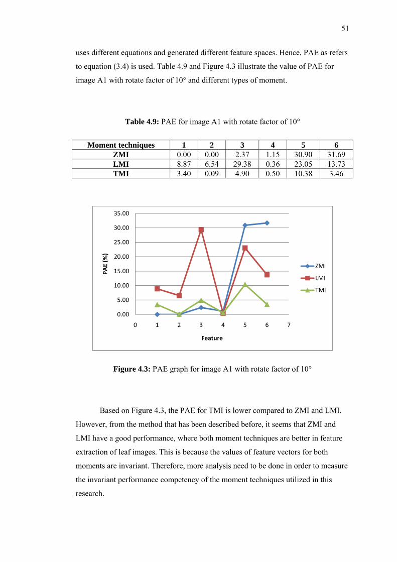
uses different equations and generated different feature spaces. Hence, PAE as refers

to equation (3.4) is used. Table 4.9 and Figure 4.3 illustrate the value of PAE for

image A1 with rotate factor of 10° and different types of moment.

Table 4.9: PAE for image A1 with rotate factor of 10°

Moment techniques 1 2 3 4 5 6

ZMI 0.00 0.00 2.37 1.15 30.90 31.69 LMI 8.87 6.54 29.38 0.36 23.05 13.73 TMI 3.40 0.09 4.90 0.50 10.38 3.46

Figure 4.3: PAE graph for image A1 with rotate factor of 10°

Based on Figure 4.3, the PAE for TMI is lower compared to ZMI and LMI.

However, from the method that has been described before, it seems that ZMI and

LMI have a good performance, where both moment techniques are better in feature

extraction of leaf images. This is because the values of feature vectors for both

moments are invariant. Therefore, more analysis need to be done in order to measure

the invariant performance competency of the moment techniques utilized in this

research.

0.00

5.00

10.00

15.00

20.00

25.00

30.00

35.00

0 1 2 3 4 5 6 7

PAE (%

)

Feature

ZMI

LMI

TMI

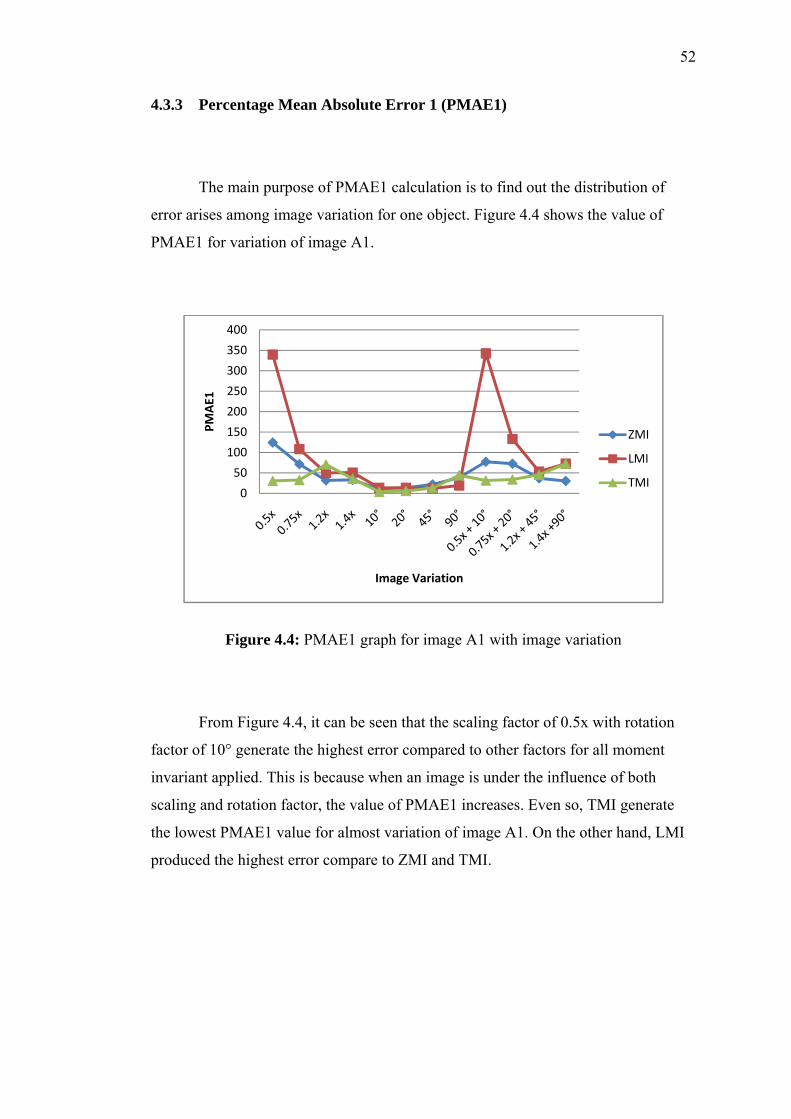
52

4.3.3 Percentage Mean Absolute Error 1 (PMAE1)

The main purpose of PMAE1 calculation is to find out the distribution of

error arises among image variation for one object. Figure 4.4 shows the value of

PMAE1 for variation of image A1.

Figure 4.4: PMAE1 graph for image A1 with image variation

From Figure 4.4, it can be seen that the scaling factor of 0.5x with rotation

factor of 10° generate the highest error compared to other factors for all moment

invariant applied. This is because when an image is under the influence of both

scaling and rotation factor, the value of PMAE1 increases. Even so, TMI generate

the lowest PMAE1 value for almost variation of image A1. On the other hand, LMI

produced the highest error compare to ZMI and TMI.

0

50

100

150

200

250

300

350

400

PMAE1

Image Variation

ZMI

LMI

TMI

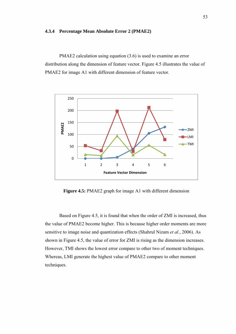
53

4.3.4 Percentage Mean Absolute Error 2 (PMAE2)

PMAE2 calculation using equation (3.6) is used to examine an error

distribution along the dimension of feature vector. Figure 4.5 illustrates the value of

PMAE2 for image A1 with different dimension of feature vector.

Figure 4.5: PMAE2 graph for image A1 with different dimension

Based on Figure 4.5, it is found that when the order of ZMI is increased, thus

the value of PMAE2 become higher. This is because higher order moments are more

sensitive to image noise and quantization effects (Shahrul Nizam et al., 2006). As

shown in Figure 4.5, the value of error for ZMI is rising as the dimension increases.

However, TMI shows the lowest error compare to other two of moment techniques.

Whereas, LMI generate the highest value of PMAE2 compare to other moment

techniques.

0

50

100

150

200

250

1 2 3 4 5 6

PMAE2

Feature Vector Dimension

ZMI

LMI

TMI

4.3.5 To

La

by using e

Table 4.10

image A1.

Ba

produced

0

20

40

60

80

100

120

TPMAE (%

) Value

otal Percen

astly, the tot

equation (3.

0 and Figure

.

Table 4

Figure 4.6

ased on the p

good perfor

ZMI

tage Mean

tal error of i

7) to measu

e 4.6 show

4.10: TPMA

Moment

Z

L

T

6: TPMAE

previous me

rmance. Ho

L

Moment T

Absolute E

image A1 fo

ure the invar

the value of

AE of differ

t techniques

ZMI

LMI

TMI

graph of di

ethod that h

owever, the v

LMI

Techniques

Error (TPM

or each mom

riant perform

f TPMAE f

rent momen

s TPMAE

46.

100

34.9

ifferent mom

has been des

value of TP

TMI

MAE)

ment techni

mance of th

for three mo

nts for imag

E value

89

.77

97

ments for im

scribed, bot

PMAE indic

iques is calc

he technique

oment techn

ge A1

mage A1

th ZMI and

cates that TM

54

culate

es.

niques of

TMI

MI

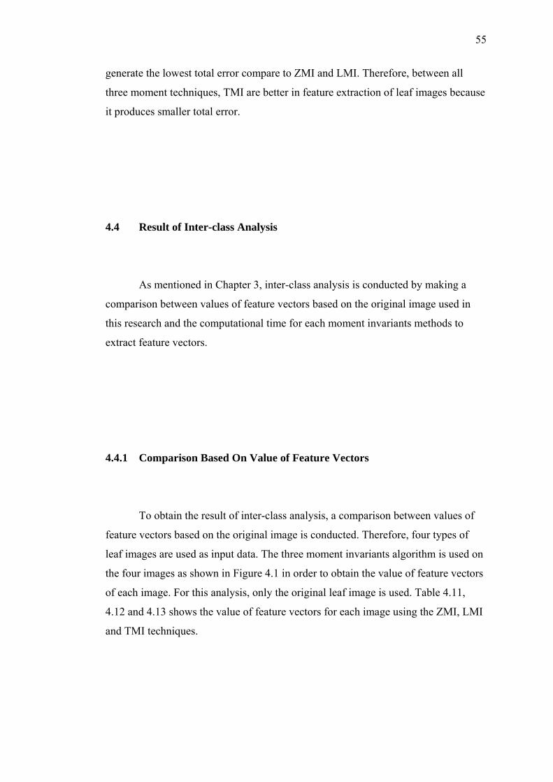
55

generate the lowest total error compare to ZMI and LMI. Therefore, between all

three moment techniques, TMI are better in feature extraction of leaf images because

it produces smaller total error.

4.4 Result of Inter-class Analysis

As mentioned in Chapter 3, inter-class analysis is conducted by making a

comparison between values of feature vectors based on the original image used in

this research and the computational time for each moment invariants methods to

extract feature vectors.

4.4.1 Comparison Based On Value of Feature Vectors

To obtain the result of inter-class analysis, a comparison between values of

feature vectors based on the original image is conducted. Therefore, four types of

leaf images are used as input data. The three moment invariants algorithm is used on

the four images as shown in Figure 4.1 in order to obtain the value of feature vectors

of each image. For this analysis, only the original leaf image is used. Table 4.11,

4.12 and 4.13 shows the value of feature vectors for each image using the ZMI, LMI

and TMI techniques.

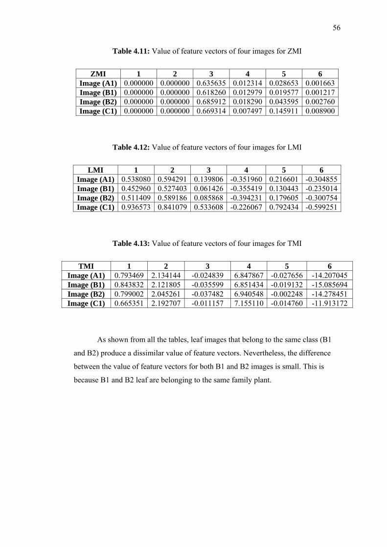
56

Table 4.11: Value of feature vectors of four images for ZMI

ZMI 1 2 3 4 5 6

Image (A1) 0.000000 0.000000 0.635635 0.012314 0.028653 0.001663Image (B1) 0.000000 0.000000 0.618260 0.012979 0.019577 0.001217Image (B2) 0.000000 0.000000 0.685912 0.018290 0.043595 0.002760Image (C1) 0.000000 0.000000 0.669314 0.007497 0.145911 0.008900

Table 4.12: Value of feature vectors of four images for LMI

LMI 1 2 3 4 5 6

Image (A1) 0.538080 0.594291 0.139806 -0.351960 0.216601 -0.304855Image (B1) 0.452960 0.527403 0.061426 -0.355419 0.130443 -0.235014Image (B2) 0.511409 0.589186 0.085868 -0.394231 0.179605 -0.300754Image (C1) 0.936573 0.841079 0.533608 -0.226067 0.792434 -0.599251

Table 4.13: Value of feature vectors of four images for TMI

TMI 1 2 3 4 5 6

Image (A1) 0.793469 2.134144 -0.024839 6.847867 -0.027656 -14.207045 Image (B1) 0.843832 2.121805 -0.035599 6.851434 -0.019132 -15.085694 Image (B2) 0.799002 2.045261 -0.037482 6.940548 -0.002248 -14.278451 Image (C1) 0.665351 2.192707 -0.011157 7.155110 -0.014760 -11.913172

As shown from all the tables, leaf images that belong to the same class (B1

and B2) produce a dissimilar value of feature vectors. Nevertheless, the difference

between the value of feature vectors for both B1 and B2 images is small. This is

because B1 and B2 leaf are belonging to the same family plant.

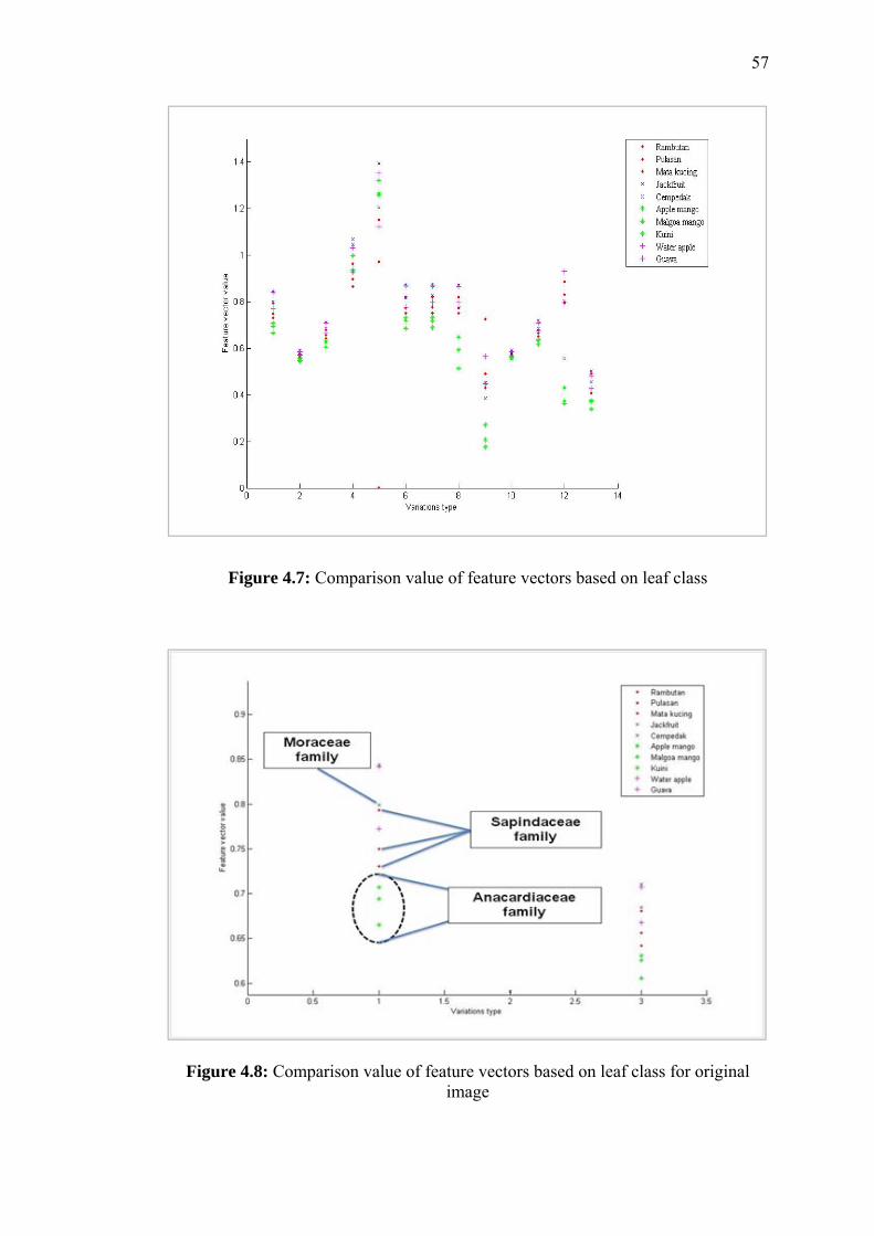
57

Figure 4.7: Comparison value of feature vectors based on leaf class

Figure 4.8: Comparison value of feature vectors based on leaf class for original image

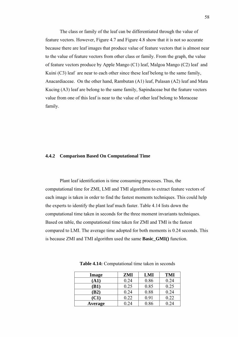
58

The class or family of the leaf can be differentiated through the value of

feature vectors. However, Figure 4.7 and Figure 4.8 show that it is not so accurate

because there are leaf images that produce value of feature vectors that is almost near

to the value of feature vectors from other class or family. From the graph, the value

of feature vectors produce by Apple Mango (C1) leaf, Malgoa Mango (C2) leaf and

Kuini (C3) leaf are near to each other since these leaf belong to the same family,

Anacardiaceae. On the other hand, Rambutan (A1) leaf, Pulasan (A2) leaf and Mata

Kucing (A3) leaf are belong to the same family, Sapindaceae but the feature vectors

value from one of this leaf is near to the value of other leaf belong to Moraceae

family.

4.4.2 Comparison Based On Computational Time

Plant leaf identification is time consuming processes. Thus, the

computational time for ZMI, LMI and TMI algorithms to extract feature vectors of

each image is taken in order to find the fastest moments techniques. This could help

the experts to identify the plant leaf much faster. Table 4.14 lists down the

computational time taken in seconds for the three moment invariants techniques.

Based on table, the computational time taken for ZMI and TMI is the fastest

compared to LMI. The average time adopted for both moments is 0.24 seconds. This

is because ZMI and TMI algorithm used the same Basic_GMI() function.

Table 4.14: Computational time taken in seconds

Image ZMI LMI TMI (A1) 0.24 0.86 0.24 (B1) 0.25 0.85 0.25 (B2) 0.24 0.88 0.24 (C1) 0.22 0.91 0.22

Average 0.24 0.86 0.24

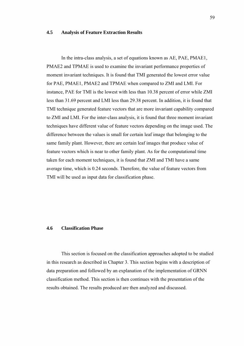
59

4.5 Analysis of Feature Extraction Results

In the intra-class analysis, a set of equations known as AE, PAE, PMAE1,

PMAE2 and TPMAE is used to examine the invariant performance properties of

moment invariant techniques. It is found that TMI generated the lowest error value

for PAE, PMAE1, PMAE2 and TPMAE when compared to ZMI and LMI. For

instance, PAE for TMI is the lowest with less than 10.38 percent of error while ZMI

less than 31.69 percent and LMI less than 29.38 percent. In addition, it is found that

TMI technique generated feature vectors that are more invariant capability compared

to ZMI and LMI. For the inter-class analysis, it is found that three moment invariant

techniques have different value of feature vectors depending on the image used. The

difference between the values is small for certain leaf image that belonging to the

same family plant. However, there are certain leaf images that produce value of

feature vectors which is near to other family plant. As for the computational time

taken for each moment techniques, it is found that ZMI and TMI have a same

average time, which is 0.24 seconds. Therefore, the value of feature vectors from

TMI will be used as input data for classification phase.

4.6 Classification Phase

This section is focused on the classification approaches adopted to be studied

in this research as described in Chapter 3. This section begins with a description of

data preparation and followed by an explanation of the implementation of GRNN

classification method. This section is then continues with the presentation of the

results obtained. The results produced are then analyzed and discussed.

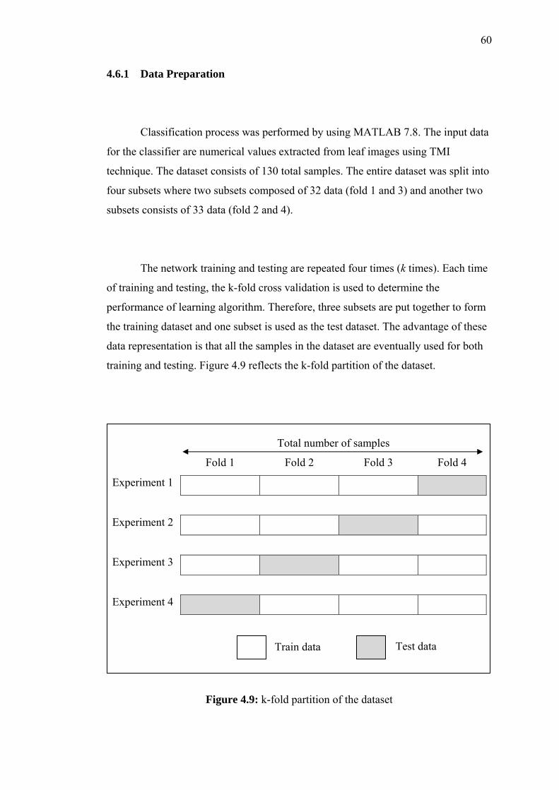
60

4.6.1 Data Preparation

Classification process was performed by using MATLAB 7.8. The input data

for the classifier are numerical values extracted from leaf images using TMI

technique. The dataset consists of 130 total samples. The entire dataset was split into

four subsets where two subsets composed of 32 data (fold 1 and 3) and another two

subsets consists of 33 data (fold 2 and 4).

The network training and testing are repeated four times (k times). Each time

of training and testing, the k-fold cross validation is used to determine the

performance of learning algorithm. Therefore, three subsets are put together to form

the training dataset and one subset is used as the test dataset. The advantage of these

data representation is that all the samples in the dataset are eventually used for both

training and testing. Figure 4.9 reflects the k-fold partition of the dataset.

Total number of samples

Fold 1 Fold 2 Fold 3 Fold 4

Experiment 1

Experiment 2

Experiment 3

Experiment 4

Figure 4.9: k-fold partition of the dataset

Train data Test data

61

4.6.2 GRNN Spread Parameters Declaration

The performance of the classifier is affected by the choice of spread

parameters. Spread value should be large enough that neurons respond strongly to

overlapping regions of the input space. The spread values are chosen 0.001, 0.005,

0.01, 0.05, and 0.1 for GRNN to achieve maximum classification rate. Each spread

value will be compared and discussed.

4.7 Classification Results of GRNN Classifier

GRNN have been used for classification scheme. The classification results of

GRNN classifier for each spread parameters are given in Table 4.15 respectively.

From Figure 4.10, it can be concluded that the percentage of correct classification

(PCC) is 100 percent for each spread parameters. However, these results shown that

each spread value do not give impact to leaf image recognition because all produced

100 percent classification rate.

62

Table 4.15: GRNN result for each spread parameters

Spread k Data

Unit Time Taken

(Second)

NCC PCC Time Average (Second)

0.001

1 32 4.49 32 100

1.49 2 33 0.60 33

3 32 0.44 32 4 33 0.42 33

0.005 1 32 0.46 32

100

0.47 2 33 0.51 33 3 32 0.51 32 4 33 0.41 33

0.01 1 32 2.42 32

100

0.98 2 33 0.50 33 3 32 0.47 32 4 33 0.48 33

0.05 1 32 0.67 32

100

0.50 2 33 0.50 33 3 32 0.44 32 4 33 0.39 33

0.1 1 32 1.12 32

100

0.87 2 33 1.24 33 3 32 0.50 32 4 33 0.62 33

k = Group of sample data

Data Unit = Number of data in sample group

63

Figure 4.10: Graph of PCC versus spread parameter value

Since all the PCC values are same, the most suitable spread parameter is

chosen based on the time average adopted by each spread values. Figure 4.11 shows

that the spread value of 0.005 acquired the quickest time average compared to others

value.

Figure 4.11: Graph of time average versus spread parameter value

0

20

40

60

80

100

120

0.001 0.005 0.01 0.05 0.1

PCC (%

)

Spread Parameter

PCC vs. Spread parameter 

0

0.2

0.4

0.6

0.8

1

1.2

1.4

1.6

0.001 0.005 0.01 0.05 0.1

Time Average

 (s)

Spread Parameter

Time Average vs. Spread Parameter 

64

4.8 Summary

This chapter discussed a comparison of effectiveness between ZMI, LMI and

TMI in representing the description of an image. From the intra-class and inter-class

analysis that have been conducted, it shows that a TMI technique is suitable for

feature extraction of leaf images. In order to continue the second stage of this

research that involved classification, the value of feature vectors from TMI will be

used as input data. This chapter then continues to discuss the performance of the

GRNN classification approach. The results of recognition and classification of leaf

images is 100 percent accuracy rate. However, the spread parameters of the GRNN

are unaffected with the leaf image recognition.

CHAPTER 5

DISCUSSION AND CONCLUSION

5.1 Introduction

The suitable moment invariant techniques for feature extraction prior to

classification task are investigated in this research. This chapter draws general

conclusion of the results obtained from this research. In addition, disadvantages of

this research will be discussed in this chapter and several potentials areas for future

work will be suggested.

5.2 Discussion of Results

With plant leaf imaging playing an increasingly prominent role in the plant

identification, the problem of extracting useful information has become important.

66

For example, leaf imaging helps to define the shape of the plant leaf and aiding in

plant recognition. To facilitate an effective and efficient review of this plant leaf

information, techniques for performing feature extraction become the key, which

lead to the main focus of this research that is to extract features from plant leaf

images using moment-based methods.

The first objective of this research is to compare the effectiveness of three

moment invariants techniques, namely ZMI, LMI and TMI to extract features from

leaf images. The effectiveness and strength of these moment invariants technique are

further studied and tested in order to see which moment invariants suitably

represents an image and would give a promising recognition rate. Then, the extracted

features from moment technique are used in training and classification using GRNN

classifier. Results of classification using these features are compared in terms of

accuracy with different spread parameters and computational time. With the

implementation of image pre-processing, feature extraction using moment invariants

technique and GRNN classification on the set of features representing the leaf

images as described in Chapter 4, the objectives of this research has been fulfilled.

In general, experiments conducted revealed the performance of the

techniques used in this research and help achieved the objectives of the research.

Moreover, it provided sufficient information and knowledge for further

investigations and future works. Experimentations from Chapter 4 have shown that

TMI are better than ZMI and LMI in representing feature extraction of leaf images.

By using Invariant Error Computation (IEC) in order to measure the invariant

performance competency of the moment techniques in this research, it shown that

TMI is suitable technique to be use for feature extraction with percentage of absolute

error is less than 10.38 percent. However, the result reveal that there are certain leaf

images produce value of feature vectors which is near to other different family of

leaf, even though the difference between the for certain leaf image that belonging to

the same family plant is small. As for classification phase, the experimental results

demonstrated that GRNN classifier produced 100 percent classification rate with

67

average computational time is 0.47 seconds. Nevertheless, the findings reveal that

the spread values do not influenced the classification rate.

5.3 Problems and Limitations of Research

There were some problems and limitations present while conducting this

research. Below are the problems and limitations:

• One of the disadvantages in this research is the use of limited sample of leaf

images. In this research, only 10 species of different plants were used and

each species includes 10 samples of leaf images. Thus, it does not generalize

the classification method.

• The occurrences of different leaf classes in the world are not taken into

account to improve the classification accuracy.

5.4 Recommendation for Future Works

Below are some suggestions that could lead to the improvement of the

classification of leaf images and some possible points that could lead to future

research.

68

• Utilization of other moment techniques that could be used in feature

extraction of an image. For instance, weighted central moments and cross

weighted moments can be applied in image analysis application.

• Utilization of other neural network model for comparison such as recurrent

neural network or Radial Basis Function (RBF). These models can be applied

in network training and classification to compare with GRNN classification

implemented in this research.

• The methodologies used in feature extraction with moment techniques and

GRNN classification can be extended to other approaches for plant

classification based on plant features of colors, textures and structures of their

bark, flower, seedling and morph.

5.5 Conclusion

The work described in this research has been concerned with the two

challenging phases in image analysis applications which are feature extraction and

classification phase. Since there is no general feature extraction method that is

available for all type of images, an experiment needs to be conducted in order to

determine the suitable methods for plant leaf images. Therefore, an investigation of

the moment invariants techniques was presented which were used to be implemented

in the feature extraction of plant leaf images. This research presents a comparison of

effectiveness between ZMI, LMI and TMI in representing the description of an

image. In this research, feature extraction methodologies using ZMI, LMI and TMI

are applied. Then, the comparison between these moment invariants technique is

presented by using IEC in terms of image representation efficiency. Based on the

experimentations performed, it can be concluded that TMI is better in representing

an image description compare with ZMI and LMI. Thus, the first objective of this

project has been achieved. Network training and classification is conducted using

69

GRNN with different spread parameters. However, these spread parameters do not

influenced the classification rate since each spread values generated 100 percent

classification rate. Future study is suggested in order to improve the recognition

accuracy of leaf images and to seek for any improvement in feature extraction where

applicable.

70

REFERENCES

Annadurai, S. and Saradha, A. (2004). Face Recognition Using Legendre Moments.

Fourth Indian Conference on Computer Vision, Graphics & Image

Processing ICVGIP 2004. 16-18 December 2004. Kolkata, India.

Belkasim, S., et al. (2004). Radial Zernike Moment Invariants. Computer and

Information Technology, 2004. CIT '04. The Fourth International

Conference. Sept 2004. Vol 1: 790- 795.

Chergui, L. and Benmohammed, M. (2008) Fuzzy Art Network for Arabic

Handwritten Recognition System. The International Arab Conference on

Information Technology (ACIT).

Dehghan, M. and Faez, K. (1997). Farsi handwritten character recognition with

moment invariants. Digital Signal Processing Proceedings, 1997. 1997 13th

International Conference. July 1997. Patras, Greece. Vol 3: 507-510.

Du, J. X. et al. (2005). Shape recognition based on radial basis probabilistic neural

network and application to plant species identification. Proceedings of 2005

International Symposium of Neural Networks. 30 May – 1 June 2005.

Chongqing, China. Vol 3498: 281-285.

Du, J. X. et al. (2006). Computer-aided plant species identification (CAPSI) based

on leaf shape matching technique. Transaction of the Institue of

Measurement and Control. Vol 28: 275-284.

Du, J. X. et al.(2007). Leaf shape based plant species recognition. Applied

Mathematics and Computation. 15 Feb 2007. Vol 185(2): 883-893.

El affar, A. et al. (2009). Krawtchouk Moment Feature Extraction for Neural Arabic

Handwritten Words Recogntion. IJCSNS International Journal of Computer

Science and Network Security. January 2009. Vol 9 (1): 417-423.

71

Flusser, J. (2006). Moment Invariants in Image Analysis. Proceedings of World

Academy of Science, Engineering and Technology. 11 February 2006. Vol

11: 196-201.

Gao, Y. et al.(2007). Identification Algorithm of Winged Insects Based On Hybrid

Moment Invariants. The 1st International Conference on Bioinformatics and

Biomedical Engineering, 2007. 6-8 July 2007. Wuhan, China. 531-534.

George, M. (2007). Radial Basis Function Neural Networks and Principal

Component Analysis for Pattern Classification. 2007 International

Conference on Computational Intelligence and Multimedia Applications. 13-

15 December 2007. Sivakasi, Tamil Nadu. 200-206.

Haddadnia, J. et al. (2001). Neural Network Based Face Recognition With Moment

Invariants. Proceedings.2001 International Conference on Image Processing.

5 – 9 November 2001. Singapore. Centre for Remote Imaging, Sensing and

Processing (CRISP), University of Singapore. Vol 1: 1018 – 1021.

Haddadnia, J. et al. (2002). A Hybrid Learning RBF Neural Network For Human

Face Recognitionwith Pseudo Zernike Moment Invariant. IEEE International

Joint Conference On Neural Network (IJCNN'02). May 2002. Honolulu,

Hawaii, USA. IEEE. 11-16.

Heymans, B. C. et al. (1991). A neural network for opuntia leaf-form recognition.

Proceedings of IEEE International Joint Conference on Neural Networks,

1991. 18-21 November 1991. Singapore. Vol 3: 2116-2121.

Hu, M. K., (1962). Visual Pattern Recognition by Moment Invariants. IRE Trans.

Inform. Theory. IT-E. 179-187.

Keyes, L. and Winstanley, A. (). Moment Invariants as a Classification Tool for

Cartographic Shapes on Large Scale Maps. 3rd AGILE Conference on

Geographic Information Science. 25-27 May 2000. Finland. 1-13.

Khotanzad, A. and Hong, Y. H. (1990) Invariant image recognition by Zernike

moments. IEEE Transactions on Pattern Analysis and Machine Intelligence.

May 1990. Vol 12 (5): 489-497.

Kotoulas, L. and Andreadis, I. (2005). Real-time computation of Zernike Moments.

IEEE Transactions on Circuits and Systems for Video Technology. June

2005. Vol 15 (6): 801-809.

72

Kunte, R. S. and Samuel R. D. S. (2006). A simple and efficient optical character

recognition system for basic symbols inprinted Kannada text. Sadhana

Bangalore. October 2007. India. Vol 32: 521-533.

Li, B. (2008). An Algorithm for License Plate Recognition Using Radial Basis

Function Neural Network. International Symposium on Computer Science

and Computional Technology, 2008. 20-22 December 2008. Shanghai,

China. Vol 1: 569-572.

Maaoui, C. et al. (2005). 2D Color Shape Recognition Using Zernike Moments.

IEEE International Confererence on Image Processing, 2005. 11-14

September 2005. Vol 3: 976-980.

McAulay, A. et al. (1991). Effect of Noise in Moment Invariant Neural Network

Aircraft Classification. Proceedings of the IEEE 1991 National Aerospace

and Electronic Conference, NAECON. 20-24 May 1991. Dayton, OH, USA:

IEEE, Vol 2: 743-749.

Mishra, C. K. et al. (2008). An Approach for Feature Extraction Using Spline

Approximation for Indian Characters (SAIC) in Recognition Engines.

TENCON 2008 IEEE Region 10 Conference. 19-21 November 2008.

Hyderabad. 1-4.

Mukundan, R. Et al. (2001) .Image Analysis by Tchebichef Moments. IEEE

Transactions on Image Processing. September 2001. Vol 20 (9): 1357-1364.

Mukundan, R. (2005). Radial Tchebichef Invariants for Pattern Recognition.

TENCON 2005 IEEE Region 10. 21-24 November 2005. Melbourne,

Australia. 1-6.

Mukundan, R., and Ramakrishnan, K. R. (1998). Moment Function in Image

Analysis. Farrer Road, Singapore: World Scientific Publishing.

Nabatchian, A. et al.(2008). Human Face Recognition Using Different Moment

Invariants: A Comparative Study. Congress on Image and Signal Processing,

2008. 27-30 May 2008. Sanya, China. Vol 3: 661-666.

Pan, F. and Keane, M. (1994). A New Set Of Moment Invariants For Handwritten

Numeral Recognition. 1994 Proceedings IEEE International Conference on

Image Processing, ICIP-94. 13 – 16 November 1994. Austin, Texas, USA :

IEEE. Vol 1: 245-249.

73

Phiasai T. et al. (2001). Face recognition system with PCA and moment invariant

method. The 2001 IEEE International Symposium on Circiuts and Systems,

ISCAS 2001, 6-9 May 2001. Sydney, NSW. Vol 2: 165-168.

Puteh Saad. (2004). Feature Extraction of Trademark Images Using Geometric

Invariant Moment and Zernike Moment-A Comparison. Chiang Mai Journal

of Science. Vol 31: 217-222.

Rani, J. S. et al. (2007). A Novel Feature Extraction Technique for Face

Recognition. International Conference on Computational Intelligence and

Multimedia Applications, 2007. 13-15 December 2007. Sivakasi, Tamil

Nadu. Vol 2: 428-435.

Sarfraz, M. et al. (2003). Offline Arabic text recognition system. The Proceedings of

IEEE International Conference on Geoemetric Modeling and Graphics-

GMAG’2003. 16 – 18 July 2003. London, England, UK: IEEE. 30 -35.

Shahrul Nizam Yaakob and Puteh Saad. (2007). Generalization Performance

Analysis between Fuzzy ARTMAP and Gaussian ARTMAP Neural

Network. Malaysian Journal of Computer Science. Vol 2: 13-22.

Teague, M. R (1980). Image Analysis Via The General Theory Of Moments. Journal

of the Optical Society of America. Vol. 70: 920-930.

Uhrig, R. E. (1995). Introduction to Artificial Neural Networks. Proceedings of the

1995 IEEE IECON 21st International Conference on Industrial Electronics,

Control and Intrumentation, 1995. 6-10 November 1995. Orlando FL. Vol 1:

33-37.

Wang, D. et al.(2002). Protein sequences classification using radial basis function

(RBF) neural networks. Proceedings of the 9th International Conference on

Neural Information Processing, 2002. 18-22 November 2002. Vol 2: 764-

768.

Wang, G. and Wang, S. (2006). Recursive computation of Tchebichef moment and

its inverse transform. The Journal of the Pattern Recognition Society. Vol 39

(1): 47-56.

Wang, W. (2008). Face Recognition Based On Radial Basis Function Neural

Networks. International Seminar on Future Information Technology and

Management Engineering, 2008. 20 November 2008. Leicestershire, UK. 41-

44.

74

Wang, X.F.et al. (2005). Recognition of Leaf Images Based on Shape Features

Using a Hypersphere Classifier. International Conference on Intelligent

Computing, 2005. 23-26 August 2005. Hefei, China. Vol 3644: 87–96.

Warren, D. (1997). Automated leaf shape description for variety testing in

chrysanthemums. Proceedings of IEEE 6th International Conference on

Image Processing and Its Applications, 1997. 14-17 July 1997. Dublin,

Ireland. Vol 2: 497-501.

Warwick, K. And Craddock, R. (1996). An introduction to Radial Basis Functions

for system identification: A comparison with other neural network methods.

Proceedings of the 35th IEEE on Decision and Control, 1996, 11-13

December 1996. Kobe, Japan. Vol 1: 464-496.

Wu, S. G. et al. (2007). A Leaf Recognition Algorithm for Plant Classification Using

Probabilistic Neural Network. 2007 IEEE International Symposium on Signal

Processing and Information Technology. 15-18 December 2007. Giza. 11-16.

Yap, P. T. et al.(2003). Image Analysis by Krawtchouk Moments. IEEE

Transactions on Image Processing. November 2003. Vol 12 (11): 1367-

1377.

Yu, P. F. and Xu D. (2008). Palmprint Recognition Based On Modified DCT

Features and RBF Neural Network. 2008 International Conference on

Machine Learning and Cybernetics. 12-15 July 2008. Kunming, China.

2982-2986.

APPENDIX A

PROJECT 1 GANTT CHART

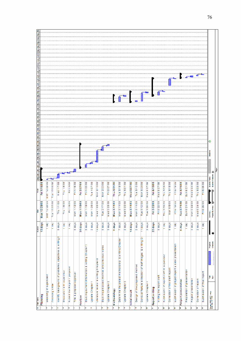
76

APPENDIX B

PROJECT 2 GANTT CHART

78

APPENDIX C

ORIGINAL LEAF IMAGES

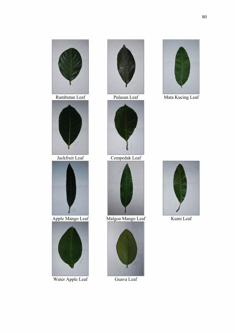
80

Rambutan Leaf Pulasan Leaf Mata Kucing Leaf

Jackfruit Leaf Cempedak Leaf

Apple Mango Leaf Malgoa Mango Leaf Kuini Leaf

Water Apple Leaf Guava Leaf

APPENDIX D

BINARY LEAF IMAGES

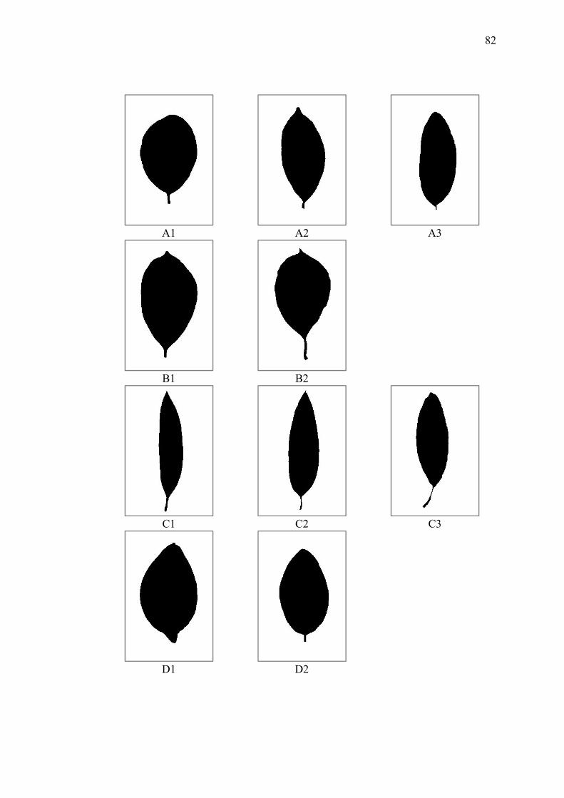
82

A1 A2 A3

B1 B2

C1 C2 C3

D1 D2

APPENDIX E

IMAGE REFERENCES

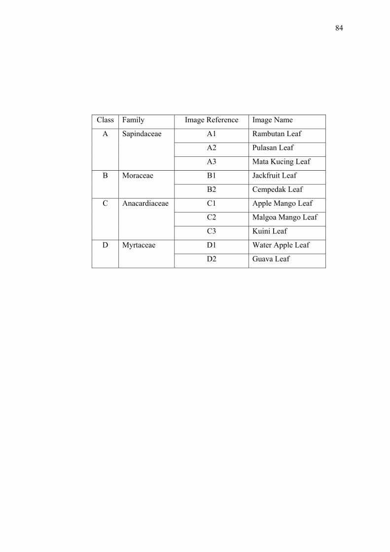
84

Class Family Image Reference Image Name

A Sapindaceae A1 Rambutan Leaf

A2 Pulasan Leaf

A3 Mata Kucing Leaf

B Moraceae B1 Jackfruit Leaf

B2 Cempedak Leaf

C Anacardiaceae C1 Apple Mango Leaf

C2 Malgoa Mango Leaf

C3 Kuini Leaf

D Myrtaceae D1 Water Apple Leaf

D2 Guava Leaf

APPENDIX F

VALUE OF FEATURE VECTORS BY ZMI

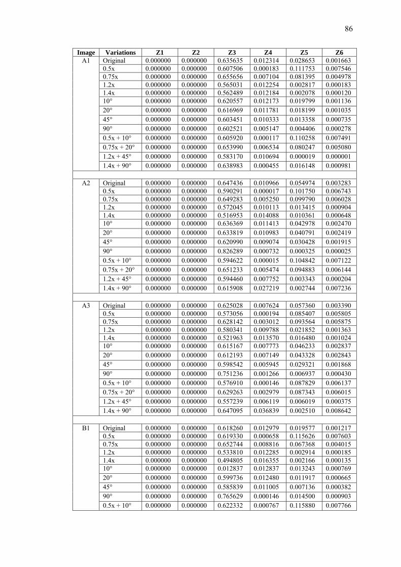
86

Image Variations Z1 Z2 Z3 Z4 Z5 Z6 A1 Original 0.000000 0.000000 0.635635 0.012314 0.028653 0.001663

0.5x 0.000000 0.000000 0.607506 0.000183 0.111753 0.007546 0.75x 0.000000 0.000000 0.655656 0.007104 0.081395 0.004978 1.2x 0.000000 0.000000 0.565031 0.012254 0.002817 0.000183 1.4x 0.000000 0.000000 0.562489 0.012184 0.002078 0.000120 10° 0.000000 0.000000 0.620557 0.012173 0.019799 0.001136 20° 0.000000 0.000000 0.616969 0.011781 0.018199 0.001035 45° 0.000000 0.000000 0.603451 0.010333 0.013358 0.000735 90° 0.000000 0.000000 0.602521 0.005147 0.004406 0.000278 0.5x + 10° 0.000000 0.000000 0.605920 0.000117 0.110258 0.007491 0.75x + 20° 0.000000 0.000000 0.653990 0.006534 0.080247 0.005080 1.2x + 45° 0.000000 0.000000 0.583170 0.010694 0.000019 0.000001 1.4x + 90° 0.000000 0.000000 0.638983 0.000455 0.016148 0.000981

A2 Original 0.000000 0.000000 0.647436 0.010966 0.054974 0.003283

0.5x 0.000000 0.000000 0.590291 0.000017 0.101750 0.006743 0.75x 0.000000 0.000000 0.649283 0.005250 0.099790 0.006028 1.2x 0.000000 0.000000 0.572045 0.010113 0.013415 0.000904 1.4x 0.000000 0.000000 0.516953 0.014088 0.010361 0.000648 10° 0.000000 0.000000 0.636369 0.011413 0.042978 0.002470 20° 0.000000 0.000000 0.633819 0.010983 0.040791 0.002419 45° 0.000000 0.000000 0.620990 0.009074 0.030428 0.001915 90° 0.000000 0.000000 0.826289 0.000732 0.000325 0.000025 0.5x + 10° 0.000000 0.000000 0.594622 0.000015 0.104842 0.007122 0.75x + 20° 0.000000 0.000000 0.651233 0.005474 0.094883 0.006144 1.2x + 45° 0.000000 0.000000 0.594460 0.007752 0.003343 0.000204 1.4x + 90° 0.000000 0.000000 0.615908 0.027219 0.002744 0.007236

A3 Original 0.000000 0.000000 0.625028 0.007624 0.057360 0.003390

0.5x 0.000000 0.000000 0.573056 0.000194 0.085407 0.005805 0.75x 0.000000 0.000000 0.628142 0.003012 0.093564 0.005875 1.2x 0.000000 0.000000 0.580341 0.009788 0.021852 0.001363 1.4x 0.000000 0.000000 0.521963 0.013570 0.016480 0.001024 10° 0.000000 0.000000 0.615167 0.007773 0.046233 0.002837 20° 0.000000 0.000000 0.612193 0.007149 0.043328 0.002843 45° 0.000000 0.000000 0.598542 0.005945 0.029321 0.001868 90° 0.000000 0.000000 0.751236 0.001266 0.006937 0.000430 0.5x + 10° 0.000000 0.000000 0.576910 0.000146 0.087829 0.006137 0.75x + 20° 0.000000 0.000000 0.629263 0.002979 0.087343 0.006015 1.2x + 45° 0.000000 0.000000 0.557239 0.006119 0.006019 0.000375 1.4x + 90° 0.000000 0.000000 0.647095 0.036839 0.002510 0.008642

B1

Original 0.000000 0.000000 0.618260 0.012979 0.019577 0.001217 0.5x 0.000000 0.000000 0.619330 0.000658 0.115626 0.007603 0.75x 0.000000 0.000000 0.652744 0.008816 0.067368 0.004015 1.2x 0.000000 0.000000 0.533810 0.012285 0.002914 0.000185 1.4x 0.000000 0.000000 0.494805 0.016355 0.002166 0.000135 10° 0.000000 0.000000 0.012837 0.012837 0.013243 0.000769 20° 0.000000 0.000000 0.599736 0.012480 0.011917 0.000665 45° 0.000000 0.000000 0.585839 0.011005 0.007136 0.000382 90° 0.000000 0.000000 0.765629 0.000146 0.014500 0.000903 0.5x + 10° 0.000000 0.000000 0.622332 0.000767 0.115880 0.007766

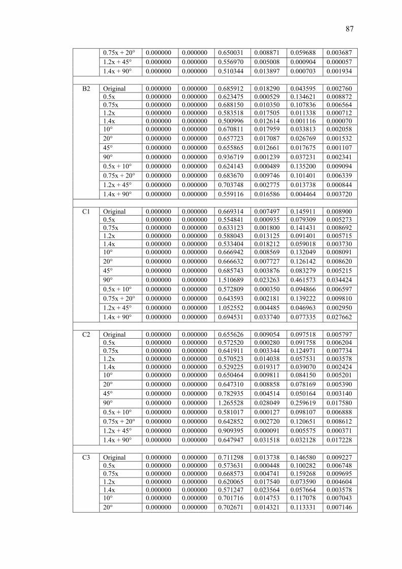
87

0.75x + 20° 0.000000 0.000000 0.650031 0.008871 0.059688 0.003687 1.2x + 45° 0.000000 0.000000 0.556970 0.005008 0.000904 0.000057 1.4x + 90° 0.000000 0.000000 0.510344 0.013897 0.000703 0.001934

B2 Original 0.000000 0.000000 0.685912 0.018290 0.043595 0.002760

0.5x 0.000000 0.000000 0.623475 0.000529 0.134621 0.008872 0.75x 0.000000 0.000000 0.688150 0.010350 0.107836 0.006564 1.2x 0.000000 0.000000 0.583518 0.017505 0.011338 0.000712 1.4x 0.000000 0.000000 0.500996 0.012614 0.001116 0.000070 10° 0.000000 0.000000 0.670811 0.017959 0.033813 0.002058 20° 0.000000 0.000000 0.657723 0.017087 0.026769 0.001532 45° 0.000000 0.000000 0.655865 0.012661 0.017675 0.001107 90° 0.000000 0.000000 0.936719 0.001239 0.037231 0.002341 0.5x + 10° 0.000000 0.000000 0.624143 0.000489 0.135200 0.009094 0.75x + 20° 0.000000 0.000000 0.683670 0.009746 0.101401 0.006339 1.2x + 45° 0.000000 0.000000 0.703748 0.002775 0.013738 0.000844 1.4x + 90° 0.000000 0.000000 0.559116 0.016586 0.004464 0.003720

C1 Original 0.000000 0.000000 0.669314 0.007497 0.145911 0.008900

0.5x 0.000000 0.000000 0.554841 0.000935 0.079309 0.005273 0.75x 0.000000 0.000000 0.633123 0.001800 0.141431 0.008692 1.2x 0.000000 0.000000 0.588043 0.013125 0.091401 0.005715 1.4x 0.000000 0.000000 0.533404 0.018212 0.059018 0.003730 10° 0.000000 0.000000 0.666942 0.008569 0.132049 0.008091 20° 0.000000 0.000000 0.666632 0.007727 0.126142 0.008620 45° 0.000000 0.000000 0.685743 0.003876 0.083279 0.005215 90° 0.000000 0.000000 1.510689 0.023263 0.461573 0.034424 0.5x + 10° 0.000000 0.000000 0.572809 0.000350 0.094866 0.006597 0.75x + 20° 0.000000 0.000000 0.643593 0.002181 0.139222 0.009810 1.2x + 45° 0.000000 0.000000 1.052552 0.004485 0.046963 0.002950 1.4x + 90° 0.000000 0.000000 0.694531 0.033740 0.077335 0.027662

C2

Original 0.000000 0.000000 0.655626 0.009054 0.097518 0.005797 0.5x 0.000000 0.000000 0.572520 0.000280 0.091758 0.006204 0.75x 0.000000 0.000000 0.641911 0.003344 0.124971 0.007734 1.2x 0.000000 0.000000 0.570523 0.014038 0.057531 0.003578 1.4x 0.000000 0.000000 0.529225 0.019317 0.039070 0.002424 10° 0.000000 0.000000 0.650464 0.009811 0.084150 0.005201 20° 0.000000 0.000000 0.647310 0.008858 0.078169 0.005390 45° 0.000000 0.000000 0.782935 0.004514 0.050164 0.003140 90° 0.000000 0.000000 1.265528 0.028049 0.259619 0.017580 0.5x + 10° 0.000000 0.000000 0.581017 0.000127 0.098107 0.006888 0.75x + 20° 0.000000 0.000000 0.642852 0.002720 0.120651 0.008612 1.2x + 45° 0.000000 0.000000 0.909395 0.000091 0.005575 0.000371 1.4x + 90° 0.000000 0.000000 0.647947 0.031518 0.032128 0.017228

C3

Original 0.000000 0.000000 0.711298 0.013738 0.146580 0.009227 0.5x 0.000000 0.000000 0.573631 0.000448 0.100282 0.006748 0.75x 0.000000 0.000000 0.668573 0.004741 0.159268 0.009695 1.2x 0.000000 0.000000 0.620065 0.017540 0.073590 0.004604 1.4x 0.000000 0.000000 0.571247 0.023564 0.057664 0.003578 10° 0.000000 0.000000 0.701716 0.014753 0.117078 0.007043 20° 0.000000 0.000000 0.702671 0.014321 0.113331 0.007146

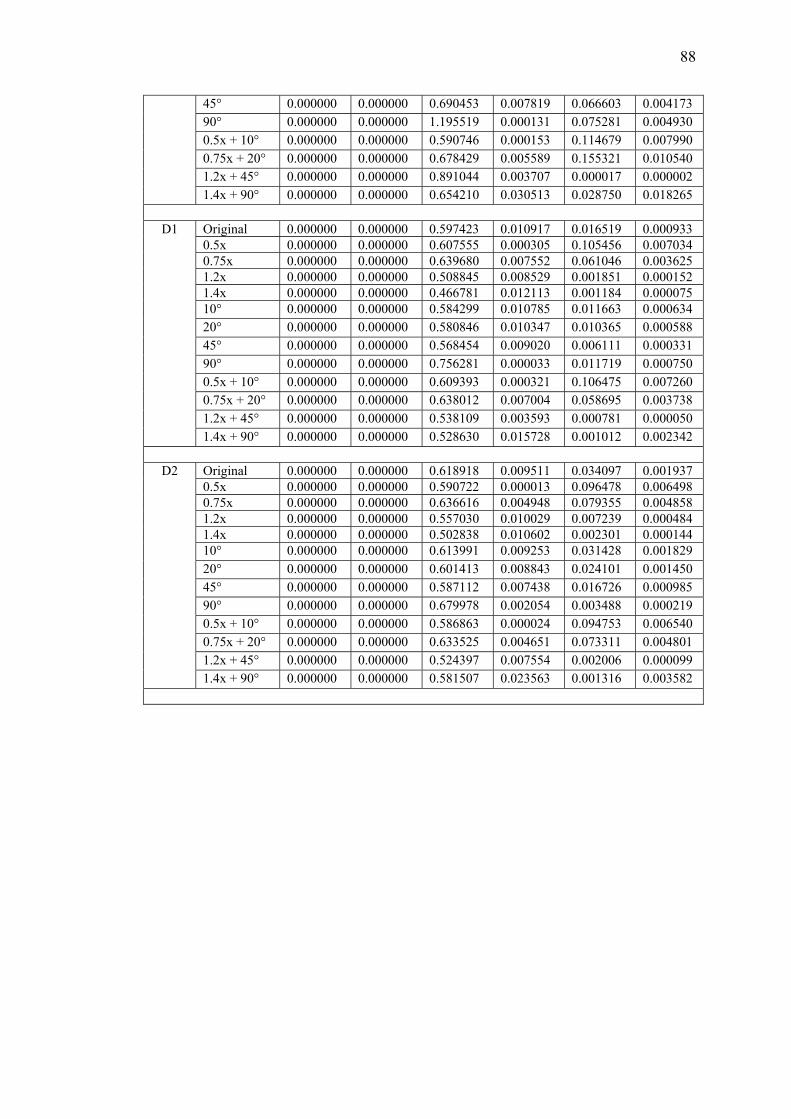
88

45° 0.000000 0.000000 0.690453 0.007819 0.066603 0.004173 90° 0.000000 0.000000 1.195519 0.000131 0.075281 0.004930 0.5x + 10° 0.000000 0.000000 0.590746 0.000153 0.114679 0.007990 0.75x + 20° 0.000000 0.000000 0.678429 0.005589 0.155321 0.010540 1.2x + 45° 0.000000 0.000000 0.891044 0.003707 0.000017 0.000002 1.4x + 90° 0.000000 0.000000 0.654210 0.030513 0.028750 0.018265

D1 Original 0.000000 0.000000 0.597423 0.010917 0.016519 0.000933

0.5x 0.000000 0.000000 0.607555 0.000305 0.105456 0.007034 0.75x 0.000000 0.000000 0.639680 0.007552 0.061046 0.003625 1.2x 0.000000 0.000000 0.508845 0.008529 0.001851 0.000152 1.4x 0.000000 0.000000 0.466781 0.012113 0.001184 0.000075 10° 0.000000 0.000000 0.584299 0.010785 0.011663 0.000634 20° 0.000000 0.000000 0.580846 0.010347 0.010365 0.000588 45° 0.000000 0.000000 0.568454 0.009020 0.006111 0.000331 90° 0.000000 0.000000 0.756281 0.000033 0.011719 0.000750 0.5x + 10° 0.000000 0.000000 0.609393 0.000321 0.106475 0.007260 0.75x + 20° 0.000000 0.000000 0.638012 0.007004 0.058695 0.003738 1.2x + 45° 0.000000 0.000000 0.538109 0.003593 0.000781 0.000050 1.4x + 90° 0.000000 0.000000 0.528630 0.015728 0.001012 0.002342

D2

Original 0.000000 0.000000 0.618918 0.009511 0.034097 0.001937 0.5x 0.000000 0.000000 0.590722 0.000013 0.096478 0.006498 0.75x 0.000000 0.000000 0.636616 0.004948 0.079355 0.004858 1.2x 0.000000 0.000000 0.557030 0.010029 0.007239 0.000484 1.4x 0.000000 0.000000 0.502838 0.010602 0.002301 0.000144 10° 0.000000 0.000000 0.613991 0.009253 0.031428 0.001829 20° 0.000000 0.000000 0.601413 0.008843 0.024101 0.001450 45° 0.000000 0.000000 0.587112 0.007438 0.016726 0.000985 90° 0.000000 0.000000 0.679978 0.002054 0.003488 0.000219 0.5x + 10° 0.000000 0.000000 0.586863 0.000024 0.094753 0.006540 0.75x + 20° 0.000000 0.000000 0.633525 0.004651 0.073311 0.004801 1.2x + 45° 0.000000 0.000000 0.524397 0.007554 0.002006 0.000099 1.4x + 90° 0.000000 0.000000 0.581507 0.023563 0.001316 0.003582

APPENDIX G

VALUE OF FEATURE VECTORS BY LMI

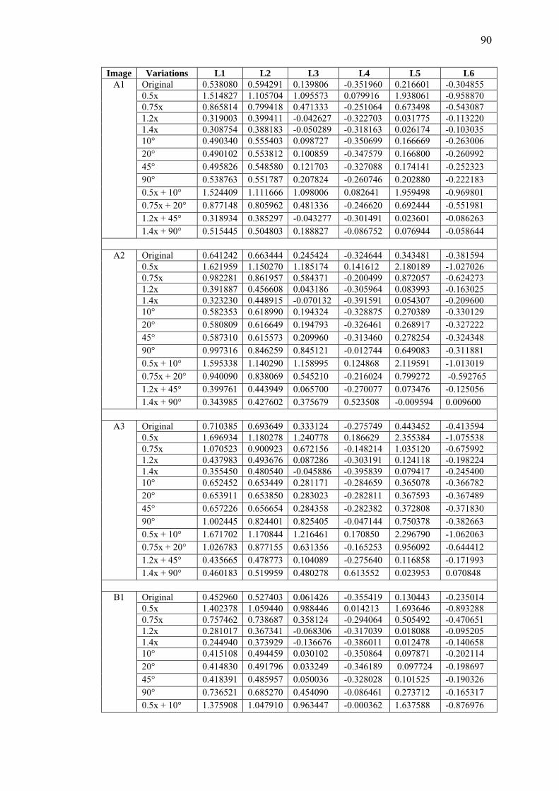
90

Image Variations L1 L2 L3 L4 L5 L6 A1 Original 0.538080 0.594291 0.139806 -0.351960 0.216601 -0.304855

0.5x 1.514827 1.105704 1.095573 0.079916 1.938061 -0.958870 0.75x 0.865814 0.799418 0.471333 -0.251064 0.673498 -0.543087 1.2x 0.319003 0.399411 -0.042627 -0.322703 0.031775 -0.113220 1.4x 0.308754 0.388183 -0.050289 -0.318163 0.026174 -0.103035 10° 0.490340 0.555403 0.098727 -0.350699 0.166669 -0.263006 20° 0.490102 0.553812 0.100859 -0.347579 0.166800 -0.260992 45° 0.495826 0.548580 0.121703 -0.327088 0.174141 -0.252323 90° 0.538763 0.551787 0.207824 -0.260746 0.202880 -0.222183 0.5x + 10° 1.524409 1.111666 1.098006 0.082641 1.959498 -0.969801 0.75x + 20° 0.877148 0.805962 0.481336 -0.246620 0.692444 -0.551981 1.2x + 45° 0.318934 0.385297 -0.043277 -0.301491 0.023601 -0.086263 1.4x + 90° 0.515445 0.504803 0.188827 -0.086752 0.076944 -0.058644

A2 Original 0.641242 0.663444 0.245424 -0.324644 0.343481 -0.381594

0.5x 1.621959 1.150270 1.185174 0.141612 2.180189 -1.027026 0.75x 0.982281 0.861957 0.584371 -0.200499 0.872057 -0.624273 1.2x 0.391887 0.456608 0.043186 -0.305964 0.083993 -0.163025 1.4x 0.323230 0.448915 -0.070132 -0.391591 0.054307 -0.209600 10° 0.582353 0.618990 0.194324 -0.328875 0.270389 -0.330129 20° 0.580809 0.616649 0.194793 -0.326461 0.268917 -0.327222 45° 0.587310 0.615573 0.209960 -0.313460 0.278254 -0.324348 90° 0.997316 0.846259 0.845121 -0.012744 0.649083 -0.311881 0.5x + 10° 1.595338 1.140290 1.158995 0.124868 2.119591 -1.013019 0.75x + 20° 0.940090 0.838069 0.545210 -0.216024 0.799272 -0.592765 1.2x + 45° 0.399761 0.443949 0.065700 -0.270077 0.073476 -0.125056 1.4x + 90° 0.343985 0.427602 0.375679 0.523508 -0.009594 0.009600

A3 Original 0.710385 0.693649 0.333124 -0.275749 0.443452 -0.413594

0.5x 1.696934 1.180278 1.240778 0.186629 2.355384 -1.075538 0.75x 1.070523 0.900923 0.672156 -0.148214 1.035120 -0.675992 1.2x 0.437983 0.493676 0.087286 -0.303191 0.124118 -0.198224 1.4x 0.355450 0.480540 -0.045886 -0.395839 0.079417 -0.245400 10° 0.652452 0.653449 0.281171 -0.284659 0.365078 -0.366782 20° 0.653911 0.653850 0.283023 -0.282811 0.367593 -0.367489 45° 0.657226 0.656654 0.284358 -0.282382 0.372808 -0.371830 90° 1.002445 0.824401 0.825405 -0.047144 0.750378 -0.382663 0.5x + 10° 1.671702 1.170844 1.216461 0.170850 2.296790 -1.062063 0.75x + 20° 1.026783 0.877155 0.631356 -0.165253 0.956092 -0.644412 1.2x + 45° 0.435665 0.478773 0.104089 -0.275640 0.116858 -0.171993 1.4x + 90° 0.460183 0.519959 0.480278 0.613552 0.023953 0.070848

B1

Original 0.452960 0.527403 0.061426 -0.355419 0.130443 -0.235014 0.5x 1.402378 1.059440 0.988446 0.014213 1.693646 -0.893288 0.75x 0.757462 0.738687 0.358124 -0.294064 0.505492 -0.470651 1.2x 0.281017 0.367341 -0.068306 -0.317039 0.018088 -0.095205 1.4x 0.244940 0.373929 -0.136676 -0.386011 0.012478 -0.140658 10° 0.415108 0.494459 0.030102 -0.350864 0.097871 -0.202114 20° 0.414830 0.491796 0.033249 -0.346189 0.097724 -0.198697 45° 0.418391 0.485957 0.050036 -0.328028 0.101525 -0.190326 90° 0.736521 0.685270 0.454090 -0.086461 0.273712 -0.165317 0.5x + 10° 1.375908 1.047910 0.963447 -0.000362 1.637588 -0.876976

91

0.75x + 20° 0.725999 0.715717 0.333166 -0.297529 0.459805 -0.441089 1.2x + 45° 0.299276 0.337971 -0.020784 -0.221221 0.009798 -0.035239 1.4x + 90° 0.211900 0.258073 0.196729 0.271152 -0.031042 -0.064955

B2 Original 0.511409 0.589186 0.085868 -0.394231 0.179605 -0.300754

0.5x 1.486282 1.097286 1.071795 0.057637 1.872622 -0.945718 0.75x 0.835196 0.794631 0.425712 -0.288385 0.618756 -0.539646 1.2x 0.335085 0.443222 -0.064307 -0.384797 0.047764 -0.177136 1.4x 0.248542 0.345937 -0.099740 -0.326578 0.009249 -0.088886 10° 0.479601 0.561462 0.059902 -0.389758 0.148656 -0.270882 20° 0.466808 0.546931 0.054812 -0.380710 0.137399 -0.254589 45° 0.499334 0.552036 0.116189 -0.336225 0.162649 -0.241111 90° 0.912355 0.870470 0.510074 -0.135355 0.359077 -0.237592 0.5x + 10° 1.486694 1.098201 1.069958 0.056798 1.873578 -0.947839 0.75x + 20° 0.832680 0.789613 0.428680 -0.282611 0.615609 -0.531808 1.2x + 45° 0.426649 0.446168 -0.015119 -0.208795 0.022181 -0.053438 1.4x + 90° 0.210707 0.325621 0.190891 0.344740 -0.011732 -0.071131

C1 Original 0.936573 0.841079 0.533608 -0.226067 0.792434 -0.599251

0.5x 1.873779 1.248181 1.398479 0.294442 2.777145 -1.177828 0.75x 1.290898 1.012691 0.875217 -0.049996 1.461507 -0.830371 1.2x 0.606622 0.692347 0.134396 -0.402445 0.351857 -0.505404 1.4x 0.498579 0.703543 -0.059848 -0.549489 0.256142 -0.638221 10° 0.849270 0.788984 0.452392 -0.253828 0.649316 -0.532236 20° 0.847819 0.786311 0.453707 -0.250967 0.647445 -0.528147 45° 1.000277 0.839586 0.690067 -0.135147 0.856884 -0.529951 90° 3.550078 3.095672 4.445548 1.226387 3.863485 -0.986985 0.5x + 10° 1.763706 1.206235 1.305510 0.226733 2.511576 -1.112816 0.75x + 20° 1.209821 0.973809 0.801543 -0.089838 1.298798 -0.775307 1.2x + 45° 1.380908 1.112799 1.400588 0.147387 1.188087 -0.468722 1.4x + 90° 0.324841 0.795302 0.653622 1.108176 -0.036508 0.283184

C2

Original 0.774654 0.742292 0.384206 -0.274813 0.533642 -0.473224 0.5x 1.745294 1.199008 1.288755 0.215732 2.468099 -1.102047 0.75x 1.125224 0.931779 0.723881 -0.129478 1.135077 -0.716920 1.2x 0.509095 0.619776 0.057188 -0.416527 0.230375 -0.413384 1.4x 0.427174 0.633813 -0.097394 -0.542907 0.167882 -0.525175 10° 0.701735 0.694009 0.317519 -0.290717 0.428406 -0.414631 20° 0.700480 0.690633 0.320087 -0.285923 0.427392 -0.409874 45° 0.981153 0.823057 0.760502 -0.097272 0.737626 -0.413811 90° 2.486116 2.227663 2.767775 1.014159 2.022915 -0.324192 0.5x + 10° 1.685112 1.176273 1.232305 0.178421 2.327123 -1.068917 0.75x + 20° 1.120460 0.927996 0.719941 -0.129085 1.126875 -0.711801 1.2x + 45° 0.867053 0.815427 0.530764 -0.007002 0.306329 -0.151412 1.4x + 90° 0.288652 0.568322 0.519491 0.808615 -0.046925 0.060713

C3

Original 0.793129 0.778963 0.369529 -0.321013 0.551079 -0.523954 0.5x 1.815422 1.223073 1.371503 0.261876 2.633198 -1.131643 0.75x 1.137358 0.948176 0.729548 -0.142885 1.152563 -0.739900 1.2x 0.510357 0.612226 0.065434 -0.416633 0.216075 -0.382264 1.4x 0.426197 0.621426 -0.091969 -0.541428 0.156279 -0.487894 10° 0.705515 0.718289 0.291611 -0.336927 0.423857 -0.447076 20° 0.705646 0.711596 0.303632 -0.325013 0.423866 -0.434689

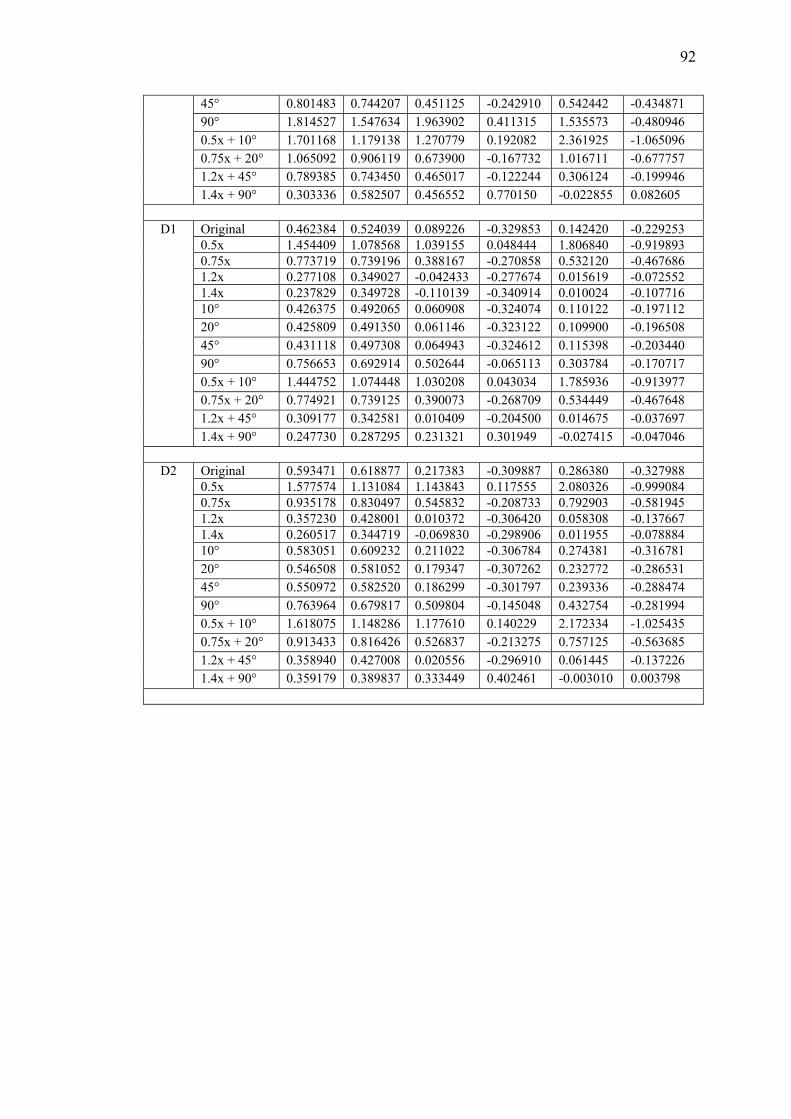
92

45° 0.801483 0.744207 0.451125 -0.242910 0.542442 -0.434871 90° 1.814527 1.547634 1.963902 0.411315 1.535573 -0.480946 0.5x + 10° 1.701168 1.179138 1.270779 0.192082 2.361925 -1.065096 0.75x + 20° 1.065092 0.906119 0.673900 -0.167732 1.016711 -0.677757 1.2x + 45° 0.789385 0.743450 0.465017 -0.122244 0.306124 -0.199946 1.4x + 90° 0.303336 0.582507 0.456552 0.770150 -0.022855 0.082605

D1 Original 0.462384 0.524039 0.089226 -0.329853 0.142420 -0.229253

0.5x 1.454409 1.078568 1.039155 0.048444 1.806840 -0.919893 0.75x 0.773719 0.739196 0.388167 -0.270858 0.532120 -0.467686 1.2x 0.277108 0.349027 -0.042433 -0.277674 0.015619 -0.072552 1.4x 0.237829 0.349728 -0.110139 -0.340914 0.010024 -0.107716 10° 0.426375 0.492065 0.060908 -0.324074 0.110122 -0.197112 20° 0.425809 0.491350 0.061146 -0.323122 0.109900 -0.196508 45° 0.431118 0.497308 0.064943 -0.324612 0.115398 -0.203440 90° 0.756653 0.692914 0.502644 -0.065113 0.303784 -0.170717 0.5x + 10° 1.444752 1.074448 1.030208 0.043034 1.785936 -0.913977 0.75x + 20° 0.774921 0.739125 0.390073 -0.268709 0.534449 -0.467648 1.2x + 45° 0.309177 0.342581 0.010409 -0.204500 0.014675 -0.037697 1.4x + 90° 0.247730 0.287295 0.231321 0.301949 -0.027415 -0.047046

D2

Original 0.593471 0.618877 0.217383 -0.309887 0.286380 -0.327988 0.5x 1.577574 1.131084 1.143843 0.117555 2.080326 -0.999084 0.75x 0.935178 0.830497 0.545832 -0.208733 0.792903 -0.581945 1.2x 0.357230 0.428001 0.010372 -0.306420 0.058308 -0.137667 1.4x 0.260517 0.344719 -0.069830 -0.298906 0.011955 -0.078884 10° 0.583051 0.609232 0.211022 -0.306784 0.274381 -0.316781 20° 0.546508 0.581052 0.179347 -0.307262 0.232772 -0.286531 45° 0.550972 0.582520 0.186299 -0.301797 0.239336 -0.288474 90° 0.763964 0.679817 0.509804 -0.145048 0.432754 -0.281994 0.5x + 10° 1.618075 1.148286 1.177610 0.140229 2.172334 -1.025435 0.75x + 20° 0.913433 0.816426 0.526837 -0.213275 0.757125 -0.563685 1.2x + 45° 0.358940 0.427008 0.020556 -0.296910 0.061445 -0.137226 1.4x + 90° 0.359179 0.389837 0.333449 0.402461 -0.003010 0.003798

APPENDIX H

VALUE OF FEATURE VECTORS BY TMI

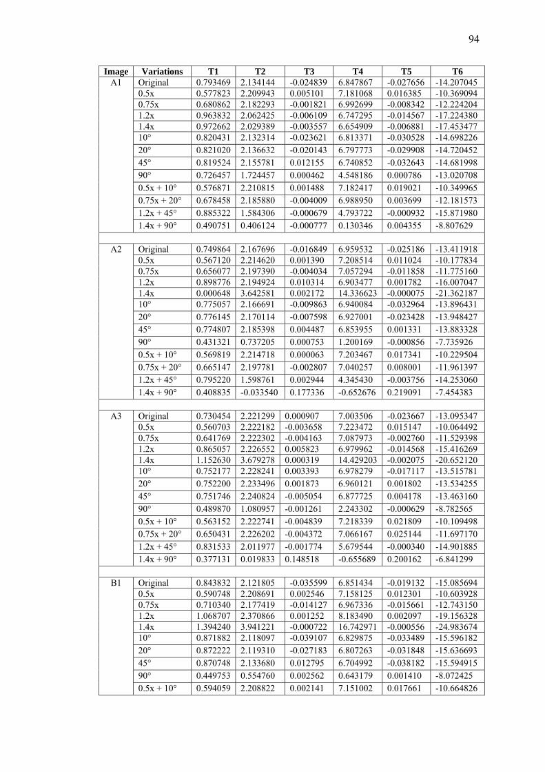
94

Image Variations T1 T2 T3 T4 T5 T6 A1 Original 0.793469 2.134144 -0.024839 6.847867 -0.027656 -14.207045

0.5x 0.577823 2.209943 0.005101 7.181068 0.016385 -10.369094 0.75x 0.680862 2.182293 -0.001821 6.992699 -0.008342 -12.224204 1.2x 0.963832 2.062425 -0.006109 6.747295 -0.014567 -17.224380 1.4x 0.972662 2.029389 -0.003557 6.654909 -0.006881 -17.453477 10° 0.820431 2.132314 -0.023621 6.813371 -0.030528 -14.698226 20° 0.821020 2.136632 -0.020143 6.797773 -0.029908 -14.720452 45° 0.819524 2.155781 0.012155 6.740852 -0.032643 -14.681998 90° 0.726457 1.724457 0.000462 4.548186 0.000786 -13.020708 0.5x + 10° 0.576871 2.210815 0.001488 7.182417 0.019021 -10.349965 0.75x + 20° 0.678458 2.185880 -0.004009 6.988950 0.003699 -12.181573 1.2x + 45° 0.885322 1.584306 -0.000679 4.793722 -0.000932 -15.871980 1.4x + 90° 0.490751 0.406124 -0.000777 0.130346 0.004355 -8.807629

A2 Original 0.749864 2.167696 -0.016849 6.959532 -0.025186 -13.411918

0.5x 0.567120 2.214620 0.001390 7.208514 0.011024 -10.177834 0.75x 0.656077 2.197390 -0.004034 7.057294 -0.011858 -11.775160 1.2x 0.898776 2.194924 0.010314 6.903477 0.001782 -16.007047 1.4x 0.000648 3.642581 0.002172 14.336623 -0.000075 -21.362187 10° 0.775057 2.166691 -0.009863 6.940084 -0.032964 -13.896431 20° 0.776145 2.170114 -0.007598 6.927001 -0.023428 -13.948427 45° 0.774807 2.185398 0.004487 6.853955 0.001331 -13.883328 90° 0.431321 0.737205 0.000753 1.200169 -0.000856 -7.735926 0.5x + 10° 0.569819 2.214718 0.000063 7.203467 0.017341 -10.229504 0.75x + 20° 0.665147 2.197781 -0.002807 7.040257 0.008001 -11.961397 1.2x + 45° 0.795220 1.598761 0.002944 4.345430 -0.003756 -14.253060 1.4x + 90° 0.408835 -0.033540 0.177336 -0.652676 0.219091 -7.454383

A3 Original 0.730454 2.221299 0.000907 7.003506 -0.023667 -13.095347

0.5x 0.560703 2.222182 -0.003658 7.223472 0.015147 -10.064492 0.75x 0.641769 2.222302 -0.004163 7.087973 -0.002760 -11.529398 1.2x 0.865057 2.226552 0.005823 6.979962 -0.014568 -15.416269 1.4x 1.152630 3.679278 0.000319 14.429203 -0.002075 -20.652120 10° 0.752177 2.228241 0.003393 6.978279 -0.017117 -13.515781 20° 0.752200 2.233496 0.001873 6.960121 0.001802 -13.534255 45° 0.751746 2.240824 -0.005054 6.877725 0.004178 -13.463160 90° 0.489870 1.080957 -0.001261 2.243302 -0.000629 -8.782565 0.5x + 10° 0.563152 2.222741 -0.004839 7.218339 0.021809 -10.109498 0.75x + 20° 0.650431 2.226202 -0.004372 7.066167 0.025144 -11.697170 1.2x + 45° 0.831533 2.011977 -0.001774 5.679544 -0.000340 -14.901885 1.4x + 90° 0.377131 0.019833 0.148518 -0.655689 0.200162 -6.841299

B1

Original 0.843832 2.121805 -0.035599 6.851434 -0.019132 -15.085694 0.5x 0.590748 2.208691 0.002546 7.158125 0.012301 -10.603928 0.75x 0.710340 2.177419 -0.014127 6.967336 -0.015661 -12.743150 1.2x 1.068707 2.370866 0.001252 8.183490 0.002097 -19.156328 1.4x 1.394240 3.941221 -0.000722 16.742971 -0.000556 -24.983674 10° 0.871882 2.118097 -0.039107 6.829875 -0.033489 -15.596182 20° 0.872222 2.119310 -0.027183 6.807263 -0.031848 -15.636693 45° 0.870748 2.133680 0.012795 6.704992 -0.038182 -15.594915 90° 0.449753 0.554760 0.002562 0.643179 0.001410 -8.072425 0.5x + 10° 0.594059 2.208822 0.002141 7.151002 0.017661 -10.664826

95

0.75x + 20° 0.720227 2.176515 -0.005841 6.942665 -0.004151 -12.944421 1.2x + 45° 0.802760 1.075105 -0.000909 2.569161 0.001038 -14.392584 1.4x + 90° 0.501641 -0.079296 0.156120 -0.714813 0.183917 -9.146039

B2 Original 0.799002 2.045261 -0.037482 6.940548 -0.002248 -14.278451

0.5x 0.579796 2.199050 0.006559 7.184007 0.011944 -10.404269 0.75x 0.684512 2.144899 -0.011429 7.023082 -0.007488 -12.272005 1.2x 1.046032 2.672342 0.002382 10.035240 0.002022 -18.735330 1.4x 1.206281 2.823280 -0.003908 10.410801 0.000490 -21.618214 10° 0.818481 2.046086 -0.038335 6.929253 -0.016287 -14.625148 20° 0.827528 2.052653 -0.028385 6.894524 -0.031576 -14.832108 45° 0.774177 1.855220 -0.000363 5.729676 0.001204 -13.875641 90° 0.383848 0.392276 -0.002249 0.487362 -0.002235 -6.884242 0.5x + 10° 0.579773 2.199265 0.005240 7.183397 0.017402 -10.405364 0.75x + 20° 0.685737 2.149829 -0.005793 7.010150 0.000650 -12.318851 1.2x + 45° 0.557531 0.394589 0.001887 0.725190 0.001268 -10.001852 1.4x + 90° 0.455345 -0.223602 0.205715 -0.576310 0.207436 -8.319920

C1 Original 0.665351 2.192707 -0.011157 7.155110 -0.014760 -11.913172

0.5x 0.544853 2.218342 -0.001245 7.264560 0.008976 -9.778989 0.75x 0.605465 2.210326 -0.004804 7.185085 -0.006148 -10.870059 1.2x 0.928934 3.424438 -0.000496 13.487342 0.000557 -16.643144 1.4x 1.267279 5.825161 0.019236 28.822324 0.006830 -22.705326 10° 0.686780 2.197433 -0.010405 7.156944 -0.012354 -12.347338 20° 0.687483 2.200332 -0.007650 7.133893 0.024054 -12.411635 45° 0.594493 1.768180 -0.001217 5.044380 0.001429 -10.655211 90° 0.176744 0.153160 -0.010445 -0.048556 -0.016169 -3.172981 0.5x + 10° 0.554127 2.217660 -0.000558 7.246283 0.017948 -9.951942 0.75x + 20° 0.617234 2.210335 -0.003698 7.156539 0.031881 -11.117378 1.2x + 45° 0.362833 0.620480 -0.000221 1.148706 -0.000078 -6.509607 1.4x + 90° 0.340578 -0.131537 0.308490 -0.472099 0.252814 -6.445462

C2

Original 0.707256 2.196118 -0.005972 7.088638 -0.022300 -12.677429 0.5x 0.555850 2.218388 -0.000896 7.239572 0.013048 -9.980157 0.75x 0.630748 2.209803 -0.002267 7.135169 -0.005982 -11.332166 1.2x 0.998435 3.535786 -0.000878 13.976765 -0.002157 -17.889673 1.4x 1.321995 5.709870 -0.016961 27.828795 -0.011147 -23.702125 10° 0.730794 2.197937 -0.002271 7.080160 -0.013926 -13.149561 20° 0.731882 2.203784 0.001896 7.053351 0.018742 -13.200801 45° 0.514358 1.204551 -0.000234 2.885169 0.001036 -9.222314 90° 0.207467 0.159280 0.006873 -0.116029 -0.002136 -3.726902 0.5x + 10° 0.561519 2.219475 -0.002841 7.229597 0.021954 -10.086685 0.75x + 20° 0.632041 2.214080 -0.002320 7.119797 0.036042 -11.379373 1.2x + 45° 0.374146 0.327310 0.003072 0.277814 -0.000346 -6.711868 1.4x + 90° 0.377153 -0.105380 0.274054 -0.552529 0.239750 -7.081538

C3

Original 0.694059 2.126780 -0.027649 7.107538 -0.005755 -12.402844 0.5x 0.548776 2.209738 0.008600 7.253217 0.009741 -9.847257 0.75x 0.625510 2.181496 -0.003683 7.142840 -0.005905 -11.224167 1.2x 0.938571 3.053502 -0.000456 11.779724 0.000299 -16.816051 1.4x 1.258163 5.088730 0.003949 24.435040 -0.008239 -22.542348 10° 0.721293 2.124420 -0.019927 7.096893 -0.011887 -12.938956 20° 0.721111 2.123195 0.001328 7.078833 0.006611 -12.994534

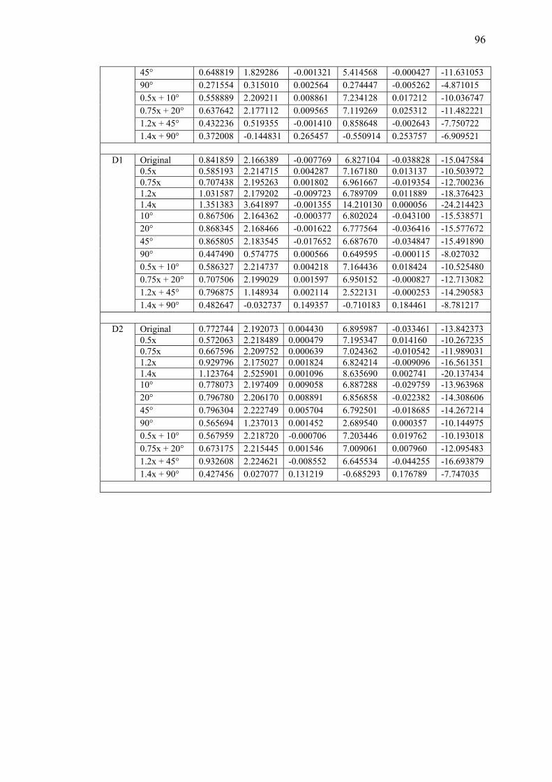
96

45° 0.648819 1.829286 -0.001321 5.414568 -0.000427 -11.631053 90° 0.271554 0.315010 0.002564 0.274447 -0.005262 -4.871015 0.5x + 10° 0.558889 2.209211 0.008861 7.234128 0.017212 -10.036747 0.75x + 20° 0.637642 2.177112 0.009565 7.119269 0.025312 -11.482221 1.2x + 45° 0.432236 0.519355 -0.001410 0.858648 -0.002643 -7.750722 1.4x + 90° 0.372008 -0.144831 0.265457 -0.550914 0.253757 -6.909521

D1 Original 0.841859 2.166389 -0.007769 6.827104 -0.038828 -15.047584

0.5x 0.585193 2.214715 0.004287 7.167180 0.013137 -10.503972 0.75x 0.707438 2.195263 0.001802 6.961667 -0.019354 -12.700236 1.2x 1.031587 2.179202 -0.009723 6.789709 0.011889 -18.376423 1.4x 1.351383 3.641897 -0.001355 14.210130 0.000056 -24.214423 10° 0.867506 2.164362 -0.000377 6.802024 -0.043100 -15.538571 20° 0.868345 2.168466 -0.001622 6.777564 -0.036416 -15.577672 45° 0.865805 2.183545 -0.017652 6.687670 -0.034847 -15.491890 90° 0.447490 0.574775 0.000566 0.649595 -0.000115 -8.027032 0.5x + 10° 0.586327 2.214737 0.004218 7.164436 0.018424 -10.525480 0.75x + 20° 0.707506 2.199029 0.001597 6.950152 -0.000827 -12.713082 1.2x + 45° 0.796875 1.148934 0.002114 2.522131 -0.000253 -14.290583 1.4x + 90° 0.482647 -0.032737 0.149357 -0.710183 0.184461 -8.781217

D2

Original 0.772744 2.192073 0.004430 6.895987 -0.033461 -13.842373 0.5x 0.572063 2.218489 0.000479 7.195347 0.014160 -10.267235 0.75x 0.667596 2.209752 0.000639 7.024362 -0.010542 -11.989031 1.2x 0.929796 2.175027 0.001824 6.824214 -0.009096 -16.561351 1.4x 1.123764 2.525901 0.001096 8.635690 0.002741 -20.137434 10° 0.778073 2.197409 0.009058 6.887288 -0.029759 -13.963968 20° 0.796780 2.206170 0.008891 6.856858 -0.022382 -14.308606 45° 0.796304 2.222749 0.005704 6.792501 -0.018685 -14.267214 90° 0.565694 1.237013 0.001452 2.689540 0.000357 -10.144975 0.5x + 10° 0.567959 2.218720 -0.000706 7.203446 0.019762 -10.193018 0.75x + 20° 0.673175 2.215445 0.001546 7.009061 0.007960 -12.095483 1.2x + 45° 0.932608 2.224621 -0.008552 6.645534 -0.044255 -16.693879 1.4x + 90° 0.427456 0.027077 0.131219 -0.685293 0.176789 -7.747035