Embed Size (px)
Citation preview

Planning and Energy Management of Energy Storage Systems in Active Distribution
Networks
By
Hussein Mohamed Hassan Abdeltawab
A thesis submitted in partial fulfillment of the requirements for the degree of
Doctor of Philosophy
in
Energy Systems
Department of Electrical and Computer Engineering
University of Alberta
© Hussein Mohamed Hassan Abdeltawab, 2017

ii
Abstract
This thesis discusses the techno-economic planning and operation of energy storage systems
in active distribution power systems. Energy storage systems (ESSs) can participate in multi-
services in the grid, such as energy arbitrage, renewable energy time-shifting, peak shaving,
power loss minimization and reactive power support. The main objective is to enable the owner
(a consumer or distribution company) to maximize profit while maintaining the power quality
and respecting the operational constraints.
In this thesis, energy storage planning is conducted by sizing and allocating both of stationary
and mobile storage. With stationary storage sizing, the system operator owns the storage which
increases the total profit by performing multi grid services including distribution system
expansion, energy arbitrage, energy loss minimization, time shifting, and reactive power support.
The optimization includes practical constraints for the battery dynamics, such as the state of
charge, and the number of charging cycles. The power flow constraints are considered, and the
bus voltage and branch ampacity are included. The sizing scheme includes other options, such as
distributed generators, static VAr compensators, and other power-balancing services. The sizing
scheme was tested by simulation on a real radial feeder in Ontario, Canada. The sizing problem
was also investigated for mobile energy storage systems (MESSs).
The second part of the thesis discusses the use of predictive energy management systems
(EMSs) for different applications. First, a predictive EMS for a hybrid wind-battery system is
discussed. The EMS provides more profit for the owner by including a practical method that
considers the battery expended-life cost. The EMS determines the optimal charging cycles and

iii
state of charge that will achieve the maximum net profit for the hybrid system owner. A
predictive EMS is also developed for a flywheel with a wind system. The flywheel regulates the
hybrid system power and its rate to comply with the grid code. The EMS considers the flywheel
power loss minimization as a factor in the optimization. A day-ahead EMS is designed for
mobile storage to define the optimal dispatching buses and powers such that the distribution
system owner’s profit is maximized. This objective is achieved by simultaneously performing
power loss minimization, reactive power support, and energy arbitrage. Finally, the thesis
demonstrates multi ESS participation in day-ahead markets by defining the robust operating
zones in the distribution system. The uncertainties of loads and renewable resources are
considered to define the safe dispatch levels for the distributed storage.
Comparative case studies, conducted on a real active distribution system in Ontario, Canada,
showed the effectiveness of the proposed planning and EMS algorithms.

iv
Preface
This thesis is an original work by Hussein Abdeltawab. As detailed in the following, some
Chapters of this thesis have been published or accepted for publication as scholarly articles in
which Prof. Yasser A.-R. I. Mohamed was the supervisory author and has contributed to
concepts formations and the manuscript composition.
Chapter 3 has been submitted as H. H. Abdeltawab and Y. A.-R. I. Mohamed, “Energy
Storage Sizing and Allocation for Distribution Network Upgrade Cost Minimization,” IEEE
Transactions on Industrial Electronics, Aug. 2016, 8-double-column pages, submitted.
Chapter 4 has been submitted as H. H. Abdeltawab and Y. A.-R. I. Mohamed, “Allocation
and Sizing of Mobile Energy Storage in Active Distribution Systems,” IEEE Transactions on
Smart Grid, Aug. 2016, 8-double-column pages, submitted.
Chapter 5 has been published as H. H. Abdeltawab and Y. A.-R. I. Mohamed, “Market-
Oriented Energy Management of a Hybrid Wind-Battery Energy Storage System via Model
Predictive Control with Constraints Optimizer,” IEEE Transactions on Industrial Electronics,
vol. 62., no. 11, pp. 6658 - 6670, Nov. 2015.
Chapter 6 has been published as H. H. Abdeltawab and Y. A.-R. I. Mohamed, “Robust
Energy Management of a Hybrid Wind and Flywheel Energy Storage System Considering
Flywheel Power Loss Minimization and Grid-Code Constraints,” IEEE Transactions on
Industrial Electronics, vol. 63 no. 7, pp. 4242 – 4254, Nov. 2016.
Chapter 7 has been submitted as H. H. Abdeltawab and Y. A.-R. I. Mohamed, “Robust
Operating Zones Identification for Independent-Energy-Storage Market Participation,”
Sustainable Energy, Grids and Networks. submitted, Aug. 2016. 12 double-column pages.

v
Chapter 8 has been published as H. H. Abdeltawab and Y. A.-R. I. Mohamed, “Mobile
Energy Storage Scheduling and Operation in Active Distribution Systems,” IEEE Transactions
on Industrial Electronics, in press. 12 double-column pages.

vi
Acknowledgements
I would like to express my deep gratitude to my supervisor, Prof. Yasser A.-R. I. Mohamed,
for his dedicated guidance and assistance during my research. I appreciate all his serious
contributions of time and discussions during my Ph.D. program.
Further, I would like to express my thanks to the examiners committee for their valued time
and interests in my thesis. I would also like to acknowledge the financial support provided by the
Alberta Innovates – Technology Futures Graduate Student Scholarship.
vii
Table of Contents
Chapter 1 .................................................................................................................................... 1
1 Introduction .......................................................................................................................... 1
1.1 Research Motivations ....................................................................................................... 1
1.2 Thesis Objectives ............................................................................................................. 2
1.3 Thesis Contributions ........................................................................................................ 3
1.4 Thesis Organization ......................................................................................................... 5
Chapter 2 .................................................................................................................................... 7
2 Literature Survey ................................................................................................................. 7
2.1 ESS Planning in Active Distribution Networks ............................................................... 8
2.1.1 Stationary Energy Storage Systems Planning ........................................................... 8
2.1.2 Mobile Energy Storage Systems Planning .............................................................. 10
2.2 Energy Management of Storage Systems ...................................................................... 10
2.2.1 Predictive EMS of Hybrid WECS-BESS System ................................................... 11
2.2.2 Predictive EMS of Hybrid WECS-FESS System ................................................... 13
2.2.3 Robust Dispatch of Multiple ESS in Active Distribution Systems ......................... 16
2.2.4 EMS of Mobile Storage System .............................................................................. 20
Chapter 3 .................................................................................................................................. 22
viii
3 Stationary Energy Storage Systems Sizing and Allocation for Multi-Services in Active
Distribution Systems ..................................................................................................................... 22
3.1 Introduction .................................................................................................................... 22
3.2 Problem Formulation ..................................................................................................... 24
3.2.1 ESS Dynamic Model ............................................................................................... 26
3.2.2 Distributed Generation ............................................................................................ 28
3.2.3 Static VAr Compensator (SVCs) ............................................................................ 30
3.2.4 Power Imbalance Solutions ..................................................................................... 31
3.2.5 Power Flow Model .................................................................................................. 32
3.3 Case Study ...................................................................................................................... 38
3.4 Results Discussion ......................................................................................................... 43
3.4.1 Economic Discussion .............................................................................................. 46
3.4.2 ESS/SVC Rating, Reactive Power Support Options ............................................... 49
3.4.3 ESS and SVC Locations .......................................................................................... 50
3.4.4 ESS for T&D Deferral, Competitive or Not? .......................................................... 51
3.5 Conclusion ...................................................................................................................... 52
Chapter 4 .................................................................................................................................. 53
4 Mobile Energy Storage Sizing and Allocation for Multi-Services Grid Support .............. 53
4.1 Introduction .................................................................................................................... 53
4.2 Problem Formulation ..................................................................................................... 54
ix
4.2.1 Mobile Storage System Structure ............................................................................ 54
4.2.2 MESS Planning Cost Function ................................................................................ 55
4.2.3 MESS Model ........................................................................................................... 58
4.2.4 Final Optimization Problem .................................................................................... 60
4.3 Proposed Algorithm ....................................................................................................... 61
4.4 Case Study ...................................................................................................................... 65
4.5 Conclusion ...................................................................................................................... 71
Chapter 5 .................................................................................................................................. 72
5 EMS of a Hybrid Wind-Battery Energy Storage System via Model Predictive Control ... 72
5.1 Introduction .................................................................................................................... 72
5.2 Hybrid WECS-BESS Description .................................................................................. 73
5.2.1 Wind Energy Conversion System (WECS) ............................................................ 74
5.2.2 Battery Energy Storage System (BESS) ................................................................. 75
5.2.3 Hybrid System State-Space Model ......................................................................... 77
5.3 Economic Perspective of Energy Management ............................................................. 78
5.3.1 Electricity Market Regulations for Renewables...................................................... 78
5.3.2 Energy Storage Cost Calculation ............................................................................ 79
5.4 Proposed Energy Management System Design ............................................................. 82
5.4.1 A Glance over MPC ................................................................................................ 83
5.4.2 Problem Formulation .............................................................................................. 84

x
5.4.3 MPC Constraints Optimizer .................................................................................... 88
5.4.4 Constraints Optimizer Algorithm ............................................................................ 90
5.5 Case study: Alberta Electricity Market .......................................................................... 94
5.5.1 Comparative Simulation Results ............................................................................. 95
5.5.2 Constraints Optimizer Sensitivity to Prediction Error ............................................ 98
5.6 Conclusions .................................................................................................................. 100
Chapter 6 ................................................................................................................................ 101
6 EMS of a Hybrid Wind – Flywheel Energy Storage System via Model Predictive Control
101
6.1 Introduction .................................................................................................................. 101
6.2 Problem Formulation ................................................................................................... 102
6.2.1 FESS Model .......................................................................................................... 106
6.2.2 The Proposed Control Structure ............................................................................ 110
6.3 The Proposed Control Algorithm ................................................................................. 113
6.3.1 Hybrid System Linearization ................................................................................ 113
6.3.2 Adaptive Hysteresis Controller (AHC) ................................................................. 117
6.3.3 Uncertainty Modes ................................................................................................ 118
6.3.4 The Two-stage Controller ..................................................................................... 121
6.4 Case Study .................................................................................................................... 123
6.5 Validation study ........................................................................................................... 129

xi
6.6 Conclusion .................................................................................................................... 133
Chapter 7 ................................................................................................................................ 135
7 Multi Energy Storage Robust Operation in Active Distribution Network ...................... 135
7.1 Introduction .................................................................................................................. 135
7.2 Problem Formulation ................................................................................................... 135
7.3 Robust Operating Zones Generation ............................................................................ 137
7.3.1 Stage A: Uncertainty Set Relaxation ..................................................................... 143
7.3.2 Stage B: Worst-Case Uncertainty Detection ......................................................... 146
7.3.3 Stage C: ROZ Determination ................................................................................ 149
7.4 Case Study .................................................................................................................... 149
7.5 Conclusions .................................................................................................................. 155
Chapter 8 ................................................................................................................................ 156
8 Mobile Energy Storage Scheduling and Operation in Active Distribution Systems ....... 156
8.1 Problem Description ..................................................................................................... 156
8.1.1 Motivation ............................................................................................................. 156
8.1.2 MESS Model ......................................................................................................... 158
8.2 Energy Management System ........................................................................................ 161
8.2.1 Transit Delay Model ............................................................................................. 162
8.2.2 MESS Dynamic Model Considering the Transit Delay ........................................ 165
8.2.3 Original EMS Problem .......................................................................................... 166

xii
8.3 Two-Stage EMS ........................................................................................................... 169
8.3.1 Stage 1 (Instantaneous Transit EMS) .................................................................... 169
8.3.2 Stage 2 (PSO Profit Maximizer) ........................................................................... 171
8.4 Case Study .................................................................................................................... 174
8.5 Conclusion .................................................................................................................... 185
Chapter 9 ................................................................................................................................ 186
9 Conclusions ...................................................................................................................... 186
9.1 Thesis Summary ........................................................................................................... 186
9.2 Future work .................................................................................................................. 188
Bibliography ........................................................................................................................... 189

xiii
List of Tables
Table 3-1 Planning input data. ................................................................................................. 42
Table 3-2. Optimization Results with different ESS technologies, and services (T1:T4) (P1 is
shown with white background whereas P2 is grey). ..................................................................... 44
Table 3-3 Biggest five loads in the Radial feeder .................................................................... 50
Table 4-1 Optimization input parameters................................................................................. 67
Table 4-2. Optimization Results With different ESS Technologies. ....................................... 68
Table 5-1 Simulation Results. .................................................................................................. 97
Table 5-2 Optimizer results in two different sample times. ..................................................... 98
Table 6-1 parameters of a single FESS unit ........................................................................... 124
Table 7-1 Fuzzy expert rules. ................................................................................................. 145
Table 7-2 RES, BESS rating. ................................................................................................. 150
Table 7-3. ROZ size and voltage violations in 100 scenarios. ............................................... 153
Table 8-1 Input data for the EMS. ......................................................................................... 177
Table 8-2 System performance comparison. .......................................................................... 181

xiv
List of Figures
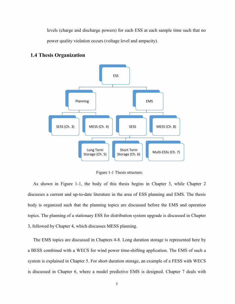
Figure 1-1 Thesis structure. ........................................................................................................ 5
Figure 3-1 System model and interconnection between the technical system and the economic
model for the planning optimization problem. ............................................................................. 25
Figure 3-2 Linearized capability curves for a circle with a different number of linearizing
lines. .............................................................................................................................................. 35
Figure 3-3 Single line diagram for the distribution feeder under study. .................................. 38
Figure 3-4 PU distance of first year (365 realization) to the 10 scenarios (centroids) depicted
as + sign, the mean distance of each scenario is shown as solid red line, while the confidence
levels are depicted by black line with a confidence level shown a s a box. ................................. 40
Figure 3-5. Yearly input data(a) PU load profile (b) PU PV generation (C) hourly market buy
price (HOEP) (d) PU wind generation. ......................................................................................... 41
Figure 3-6 Sizing results for different ESS technologies in case of P1 (Q support) (a) different
technologies cost share (b) different incomes from the investment. ............................................ 47
Figure 3-7 Comparison between total ESS size (MVA) to SVC size (MVAR) in two case (A)
ESS provides Q support (case P1) (B) SVC only provides Q support (case P2).......................... 49
Figure 4-1 MESS structure. ...................................................................................................... 54
Figure 4-2 Power conversion system cost versus rated power................................................. 57
Figure 4-3 Hybrid optimization scheme for MESS Sizing and allocation. .............................. 64
Figure 4-4 Single line diagram for the distribution feeder under study. .................................. 66
Figure 4-5 MESS rated power verses Profit. ........................................................................... 69

xv
Figure 4-6. Summer day scenario results (a) Energy buy and sell prices (b) grid purchased
power (after/before) MESS (c) MESS active and reactive Powers (d) MESS location (station).
(e) Capacity and daily number of cycles....................................................................................... 70
Figure 5-1 The hybrid system structure. .................................................................................. 73
Figure 5-2 Simplified battery model. ....................................................................................... 76
Figure 5-3 The system open-loop model. ................................................................................ 78
Figure 5-4 Relation between expended-life (EL), No. of cycles and DOD. ............................ 81
Figure 5-5 The constraints optimizer mechanism. ................................................................... 89
Figure 5-6 Flow chart of constraints optimizer and MPC operation. ...................................... 92
Figure 5-7 Simulation results for 3 cases (A, B, C) to evaluate three different controllers
(MPC1, 2, 3). ................................................................................................................................ 95
Figure 5-8 net profit change for each MPC controller in the three case studies. ..................... 96
Figure 5-9 Optimizer results at different sample times. ........................................................... 99
Figure 6-1 Hybrid system structure. ....................................................................................... 106
Figure 6-2 Hybrid system nonlinear model ........................................................................... 109
Figure 6-3 Optimization objectives at different cost function weight. .................................. 111
Figure 6-4 Hybrid system time-variant linearized model. ..................................................... 114
Figure 6-5 Linearized model performance. ............................................................................ 115
Figure 6-6 Relation of actual wind power with expected, maximum power. ........................ 119
Figure 6-7 the proposed EMS structure. ................................................................................ 122
Figure 6-8 Wind power prediction error distribution. ............................................................ 124
Figure 6-9 Simulation results comparing the performance of the traditional EMS (C1) and the
proposed MPC-based EMS (C2). ............................................................................................... 125
xvi
Figure 6-10 FESS internal dynamics- a comparison between (C1) and (C2). ....................... 127
Figure 6-11 AHC limits for SOC. .......................................................................................... 128
Figure 6-12 Opal-RT (OP 5600) real-time simulator set-up (1- OPAl-RT OP5600 real-time
simulator, 2- analog output module OP5330, 3- local host-PC, 4- a digital oscilloscope). ........ 129
Figure 6-13 System description and different process interfaces. ......................................... 130
Figure 6-14 Real-time simulation results with time scales; a- wind power (100 kW/Div.); b-
FESS power (20KW/Div.); c- SOC (5%/Div.) d- power loss (0.35 kW/div.) ........................... 133
Figure 7-1(a) Different uncertainty sets definition techniques (b) proposed risk-based
uncertainty definition technique. ................................................................................................ 141
Figure 7-2 ROZ generation framework. ................................................................................. 142
Figure 7-3 WCU detection flowchart. .................................................................................... 149
Figure 7-4 RES and load day-ahead profile with uncertainty. ............................................... 150
Figure 7-5 Voltage profile at base case. ................................................................................. 151
Figure 7-6 Desired BESS power profiles without ROZ. ........................................................ 152
Figure 7-7 RES, load uncertainty distribution for 100 scenarios each has 24 hours sample
(total 2400 uncertain sample points). .......................................................................................... 152
Figure 7-8. ROZ limits for BESS1, 2 at 30% RES-penetrations. .......................................... 154
Figure 8-1 Power Conversion System cost versus size. ......................................................... 158
Figure 8-2 Radial feeder with multi-MESS stations. ............................................................. 158
Figure 8-3 Mobile energy storage system description. .......................................................... 160
Figure 8-4 System techno-economic model structure. ........................................................... 161
Figure 8-5 Transit delay model generation. ........................................................................... 163
Figure 8-6 Transition scenarios example for a three MESS station at sample k. .................. 164

xvii
Figure 8-7 Stage 2 structure (PSO profit maximizer). ........................................................... 167
Figure 8-8 Radial feeder under study. .................................................................................... 174
Figure 8-9 Day-ahead input data. (a) Load profile. (b) RESs profiles. (c) Wholesale market
and sell prices. (d) Traffic congestion delay. .............................................................................. 176
Figure 8-10 EMS results (a)MESS Position (b) MESS active power and reactive power set (c)
Grid power and (e) SOC and Number of cycles. ........................................................................ 179
Figure 8-11 Voltage profile after and before using the MESS. ............................................. 180
Figure 8-12 Worst case bus voltage comparison (a) Bus 41 load profile and WT3 generation
(b) MESS active and reactive power (C) Bus 41volt with and without MESS reactive power
support......................................................................................................................................... 182
Figure 8-13 Comparison between reliability-based EMS with economic EMS. (a) Station
position of MESS. (B) MESS state of charge. ............................................................................ 184
xviii
List of Acronyms
BESS Battery energy storage system
DFT Discrete Fourier transform
DG Distributed generator
Disco Distribution company
Disco Distribution company
DNC Daily number of cycles
DNO Distribution network operator
DOD Depth of discharge
ELC Expended-life cost
EMS Energy management system
ESS Energy storage system
EV Electric vehicle
FESS Flywheel energy storage system
HIL Hardware-in-the-loop
ISO Independent system operator
MESS Mobile energy storage system
MPC Model predictive control
xix
NPV Net present value
PV Photovoltaic
RES Renewable energy source
RO Robust optimization
ROZ Robust operating zone
SESS Stationary energy storage system
SOC State of charge
SVC Static VAr compensator
T&D Transmission and distribution
TSO Transmission system operator
VPP Virtual power plant
WECS Wind energy conversion system

1
Chapter 1
1 Introduction
1.1 Research Motivations
The world is moving toward the extensive utilization of renewable energy as a solution to the
energy crisis. Growing electricity demand, increasing fuel prices, and greenhouse gas emissions
have led us to turn to renewable energy resources (RESs) to solve these problems.
Unfortunately, the intermittent nature of RESs leads to technical grid issues regarding the
power quality, security, and reliability [1]. Due to the increasing penetration level of RESs,
research shows that for every 10% wind penetration, a 2-4% balancing generation is needed for
a stable operation [2]. Because most energy storage systems (ESSs) are green regulation sources
with low carbon emission, they are a perfect tool for facilitating renewable energy integration in
both distribution and transmission network, as well. ESSs can provide extra services for the
grid, such as load shifting, energy arbitrage, power loss minimization, transmission, and
distribution upgrade deferral (T&D upgrade deferral), and peak shaving [3], [4].
The future of RESs growing might appear to depend on the use of ESSs; however, most
ESSs have a significant capital cost, as was recently reported in [5]. For ESSs to be a viable
solution for different grid services, optimal techno-economic planning, and operating schemes
are a must. This thesis begins by investigating the optimal sizing and siting of ESSs to achieve
optimum planning, whereas ESS operation is investigated by using some proposed energy
management schemes.

2
1.2 Thesis Objectives
This thesis aims at optimizing the planning and operation of some ESSs in the power system.
On the one hand, the optimum sizing and allocation of an ESS prevent buying an oversized unit
which reduces the capital cost. On the other hand, smart energy management decisions for ESSs
increase their life spans and provide the optimum utilization of the system.
First, the thesis objectives for the planning stage are summarized as follows.
I. The planning scheme is intended to maximize the owner’s profit as long as the power
system technical constraints are respected. The owner can be a utility company or a
customer, depending on the application, whereas the technical constraints are the grid
codes, which guarantee the power quality, system security, and reliability.
II. Optimal sizing of the ESSs power and energy rating should be performed, and the
best bus for each ESS should be allocated.
III. ESSs should be designed to be multi-tasking by achieving different objectives
simultaneously, such as energy arbitrage, energy arbitrage, reactive power support,
energy losses minimization, and, finally, feeder upgrade cost deferral.
IV. The planning scheme should consider adopting other technologies along with ESSs,
such as static VAr compensators (SVCs) or distributed generators (DGs), and also
consider load shedding and RES power curtailment as options.
V. The planning scheme should consider the prediction error in the futuristic data, such
as the load variations, renewable resources intermittency, and energy prices
fluctuations. Considering various scenarios improves the reliability of the input data,
which leads to more accurate planning results.

3
VI. The planning scheme should optimize the ESS life span by considering the batteries
state of charge and number of charging cycles.
VII. The ampacity of the network branches should be kept below the rated values, and the
voltage levels should remain within the allowable fluctuation level as permitted by
the grid code.
VIII. The previous objectives should be considered in planning mobile energy storage
systems (MESSs) as well.
Second, an effective and robust energy management system (EMS) is essential for an ESS.
The thesis objectives for the EMS stage are as follows.
I. To maximize the owner’s profit while respecting the grid code and the ESS operating
limits.
II. To make the EMS robust against predictions error and severe uncertainties.
III. To enable the EMS to satisfy the previous objectives while considering the ESS life
time constraints.
IV. To design an EMS for different applications that represent stationary energy storage
systems (SESSs) and mobile ones (MESSs).
V. To design an EMS for different applications in short duration storage (seconds,
minutes) and long duration storage (hours).
1.3 Thesis Contributions
The main thesis contribution is divided into two main parts. First, in the field of planning
ESSs, this thesis makes two main contributions:

4
I. First, this thesis proposes a sizing and siting scheme for stationary ESSs (SESSs) for
distribution system upgrade cost minimization. The T&D upgrade deferral is achieved
along with other objectives, such as energy arbitrage, power loss minimization, and
reactive power support.
II. The second contribution is the novel planning scheme for mobile ESSs (MESSs) in the
distribution system. This scheme includes MESSs for providing various grid services as
well.
In the field of ESSs operation, different energy management schemes are developed.
I. For long-term storage, a model predictive EMS scheme is designed for a hybrid
system. This system consists of a battery ESS (BESS) with a wind energy conversion
system (WECS). The BESS shifts the WECS power into more profitable hours while
taking the BESS expended-life cost into consideration.
II. For short-term storage, a model predictive EMS is designed for another hybrid
system. A flywheel energy storage system (FESS) is added to a WECS to reduce the
curtailed wind power while respecting the grid code (regarding the power limit and
rate). The proposed solution has the advantage of considering the FESS power loss
minimization during operation.
III. The MESS operation is studied by proposing a day-ahead EMS scheme that regulates
the dispatchability level and optimal locations for an MESS for an incoming day to
provide voltage support and trade energy simultaneously.
IV. Finally, the thesis proposes a robust coordination framework for distributed ESSs for
day-ahead operation. The framework defines the maximum allowable active power
5
levels (charge and discharge powers) for each ESS at each sample time such that no
power quality violation occurs (voltage level and ampacity).
1.4 Thesis Organization
Figure 1-1 Thesis structure.
As shown in Figure 1-1, the body of this thesis begins in Chapter 3, while Chapter 2
discusses a current and up-to-date literature in the area of ESS planning and EMS. The thesis
body is organized such that the planning topics are discussed before the EMS and operation
topics. The planning of a stationary ESS for distribution system upgrade is discussed in Chapter
3, followed by Chapter 4, which discusses MESS planning.
The EMS topics are discussed in Chapters 4-8. Long duration storage is represented here by
a BESS combined with a WECS for wind power time-shifting application. The EMS of such a
system is explained in Chapter 5. For short duration storage, an example of a FESS with WECS
is discussed in Chapter 6, where a model predictive EMS is designed. Chapter 7 deals with
ESS
Planning
SESS (Ch. 3) MESS (Ch. 4)
EMS
SESS
Long Term Storage (Ch. 5)
Short Term Storage (Ch. 6)
Multi-ESSs (Ch. 7)
MESS (Ch. 8)

6
multi-ESS operation in the distribution system. Finally, MESS operation for day-ahead is
optimized in Chapter 8. Lastly, Chapter 9 draws the conclusion and suggestions for future work.

7
Chapter 2
2 Literature Survey
Optimal ESS sizing (power rating and energy capacity) is an important topic when it comes
to adopting ESS for a certain grid service. ESS oversizing leads to unnecessarily high initial
capital cost whereas under-sizing will not lead to the optimal profit desired for the ESS (due to
the charging limitation or low capacity). Besides, optimal siting of ESSs is of high interest to
enable effective reactive power support and efficient power loss reduction in the distribution
system. Due to the foregoing reasons, the power research community has been investigating the
ESS planning problem thoroughly and deeply in different ESS applications. The first part of this
chapter demonstrates the current research effort in the area of ESS planning.
The optimal operation of an ESS is achievable by an EMS that satisfies the ESS owner
objectives. These objectives are economic (profit from energy market), technical (improve
power quality) or both. Utilizing the knowledge of RESs, load and market predictions lead to a
better management of the ESS in achieving the long-term objectives. The second part of this
chapter discusses the current research effort in the area of predictive EMSs for both short and
long duration storage. Furthermore, a literature survey on MESS day-ahead EMS and multiple
ESS management is presented.

8
2.1 ESS Planning in Active Distribution Networks
2.1.1 Stationary Energy Storage Systems Planning
The ESS planning has been widely discussed in the literature over different grid levels using
various optimization techniques. In the transmission system level, the work of [6] used the Tabu
search for optimal sizing of ESSs to maximize the revenue of the system considering the ESS
life cost. On the other hand, the authors of [7] proposed a three-level technique to define the
optimal ESS sizes and locations as well. Whereas the work in [6] and [7] presented
deterministic optimization algorithms for ac networks, the research in [8] revisited the sizing
problem using a stochastic optimization algorithm with a dc power flow model. On the
distribution system level, the framework in [9] proposed a stochastic optimization technique for
sizing and siting of ESSs in the power distribution system. The objective function in [9]
depends on the power quality measurements (voltage deviation, power loss, and feeders loading
factors) instead of the ESS cost. The ESS sizing problem was investigated in a microgrid system
[10] where the deterministic sizing problem maximizes the profit in both islanded and grid-
connected modes. A stochastic optimization version of [10] was discussed in [11] for an
islanded microgrid as well. Further, the authors of [12] revisited the same problem after
considering the battery exact efficiency model.
Recently, ESS sizing for frequency regulation services has been attracted much attention.
The discrete Fourier transform (DFT) was used in [13] to decompose the power imbalance
signal into different frequency ranges (acting as pass-band filters) to size different ESS
capacities (intra-hour, intraday and real time). The same technique was applied in [14] for an
islanded microgrid, where the imbalance power spectrum was shared between a diesel engine
and a fast regulating ESS. Whereas [13]- [14] do not consider the ESS cost, the authors of [15]
9
and [16] designed a search algorithm that tunes the frequency regulation bandwidth such that
the ESS cost is minimal. The partial DFT was also adopted in [17] to overcome some
drawbacks of the DFT, such as redundant computation of zero power elements, especially for
photovoltaic (PV) power.
To avoid ESS oversizing, the methods proposed in [18] and [19] use a multi-stage
optimization to tune the optimal ESS size. On the one hand, the algorithm in [18] calculated the
optimal ESS size based on hourly data, followed by a faster algorithm (with one minute-
sampled data) that takes into account the wind and PV curtailment to obtain the desired ESS
regulation capacity. On the other hand, the framework proposed in [19] tracked the minute-by-
minute power imbalance regulating effect on the battery lifetime (as the total life cycles depend
on their depth of discharge [20]). Regarding the parameters uncertainty, a probabilistic
optimization was adopted to consider the wind power uncertainty distribution in the ESS sizing
problem, such as in [21] and [22].
Recently, utilizing ESSs in transmission and distribution (T&D) deferral cost was proposed
in [23] using a probabilistic optimization. The algorithm of [23] used a genetic algorithm to size
the ESS such that the future distribution network upgrade cost is minimal by services, such as
minimizing energy losses, adopting energy arbitrage and reducing the feeder upgrade capacity.
However, the ESS was not used in either reactive power support or regulation services, which
provide better utilization of ESSs and defer possible investments in capacitor banks or SVCs.
Chapter 3 in this thesis proposes a comprehensive planning technique for ESSs in
distribution systems. This technique can be adopted by the distribution company (Disco) to
judge the viability of using ESS as a mean of T&D cost deferral with other functions, such as
energy arbitrage, reactive power support, and power loss reduction.

10
2.1.2 Mobile Energy Storage Systems Planning
Whereas the research has been focusing mainly only on the planning of stationary ESSs, the
sizing, and planning of an MESS has not yet been thoroughly investigated. On the power
industry and research levels, the MESS has witnessed some interest lately. First, an MESS
project was conducted by the Electric Power Research Institute (EPRI) in the USA [24], [25].
The project discussed designing a prototype MESS with a utility-scale size that uses the lithium-
ion technology for peak shaving. Some MESSs are also available commercially in 100, 1000
and 5000 kW units produced or rented by some companies [26] for peak shaving and improved
reliability applications. An example of an MESS prototype project is a 500 kW/1000 kWh
project for the tea industry peak shaving in China [27]. Another project under investigation is
the design a 500 kW/776 kWh MESS. This MESS uses an SCiBTM lithium-ion battery bank
for peak shaving and voltage regulation in the distribution system. The project is located in
Spain and is supported by the New Energy and Industrial Technology Development
Organization (NEDO) in Japan [28]. The work in [29] investigated the MESS sizing problem to
improve the power system reliability; however, it does not introduce a multi-tasking EMS for
the MESS, and it does not consider the load and RES uncertainty.
In Chapter 4, the problem of MESS sizing and allocation is investigated. Chapter 4 plans an
MESS owned by a Disco. The Disco considers the operation of the MESS in multi-services,
such as energy arbitrage, power loss reduction, and reactive power support services. The
algorithm in Chapter 4 decides the MESS size and optimal buses to provide such services.
2.2 Energy Management of Storage Systems
After the optimal planning and successful installation of ESSs, the user has to decide the
real-time operation strategy of the assets depending on their objectives and the storage type
11
(long- duration or short duration storage) and the storage technology (stationary or mobile). An
ESS may be owned by either the customer or the utility. Detailed applications of ESS have
reached 17 application categorized in [3]. These applications objectives vary from electric
supply services, ancillary services, grid system services, end-user service and finally, RES
integration. In this thesis, the focus is on the EMS development in the following ESS
applications:
Wind power time-shifting (Chapter 5) as a typical application for long-duration
storage.
Wind power grid integration (Chapter 6) as a typical application for short-duration
storage.
Multi-services of MESS (energy arbitrage, power loss reduction and voltage support)
as explained in Chapter 8.
For ESSs integration, Chapter 7 defines the safe dispatching levels for multi-ESSs in the
power distribution system. The following Subsections (2.2.1-2.2.4) provide a literature survey
on each of the areas above.
2.2.1 Predictive EMS of Hybrid WECS-BESS System
There have been many concerns regarding the economic revenue of renewable sources in de-
regulated markets. Energy markets are either regulated markets (with fixed tariffs) or de-
regulated markets (with variable tariffs). In a de-regulated market, the energy price is high
during peak hours, whereas it is low during off-peak hours. To maximize the WECS owner’s
profit, the owner may invest in adding a BESS to store the wind energy to sell it back during
peak hours [30], [31]. This makes the system “hybrid” and capable of performing wind power

12
time-shifting. A predictive EMS utilizes the future knowledge of both the energy price and
WECS generation to choose the optimal times to shift the WECS power.
Recently, predictive control of energy storage has gained research interest either on the lower
control level (charging level) [32] or the energy management level [33], [34]. Further, the
current development in the electrical vehicles industry [33], [35] has boosted this interest. The
model predictive control (MPC) was proposed in several studies for energy management of
hybrid systems. In [36], an EMS was proposed as an MPC for an isolated hybrid power system
composed of a WECS and BESS. The MPC aims at dispatching the WECS by regulating the
BESS power to the desired set-point. The problem was formulated as minimizing a quadratic
cost function of the power regulation error. However, the regulation constraints were taken as
the BESS power limits and the state of charge (SOC). No constraints on the BESS daily number
of cycles (DNC) were considered which may lead to an overcharging and rapid shortage in the
battery life. A decentralized MPC for a PV, WECS and BESS stand-alone system was designed
in [37]. The controller aimed at minimizing a multi-objective cost function that includes the
power imbalance, depth of discharge (DOD) and the PV power during the incoming 24-hour
period. Unfortunately, the choice of the weights of this cost function is empirical, which lacks a
systematic design approach for different systems. Further, as the design model is nonlinear,
non-convex optimization techniques were used to solve this problem. Because reaching a
feasible solution is highly related to the weights of the cost function and the initial system
conditions, a stopping criterion was used to skip the algorithm after a fixed number of iterations
if no feasible solution is reached. In [30], an EMS was designed as an MPC for a hybrid system
(PV+BESS). The controller aimed at maximizing the profit by exploiting the market diurnal
price difference. In the case of violating the pre-contracted power commitment, a penalty is paid

13
by the system owner. This penalty was taken into account as a cost in the MPC problem. The
work in [30] neglected the storage cost; however, this cost value is nontrivial and can change
the overall control strategy [38]. Moreover, although the SOC and the BESS power constraints
were considered, the DNC constraint was not included. Recently, this point was considered in
[31]. The authors of [31] considered that the optimal DNC is fixed at one cycle/day. The
charge/discharge periods were optimized using a two-stage iterative algorithm. However, the
unity DNC is only optimal with special wind power and market patterns, and this is not the
general case due to the high volatility of the market [39] and the variable daily wind power
patterns. Depending on these patterns, it may be more appropriate to allow the DNC to vary
from one cycle/day.
To address the shortages above in the previous studies, Chapter 5 proposes an EMS for a
hybrid power system composed of a WECS and BESS. The EMS is designed as a real-time
MPC that maximizes the owner’s profit by performing wind power time-shifting [40] while
considering the exact BESS expended-life cost.
2.2.2 Predictive EMS of Hybrid WECS-FESS System
The short-term storage can improve the wind power integration by improving wind power
quality which is achieved by limiting the wind power maximum magnitude and ramp rate. A
FESS is an effective short-duration storage with a high power density that enables covering
peak loads for short times [41]. FESSs start to replace uninterruptable power supply (UPS) units
that are combined with a backup diesel generator. FESSs can replace an expensive 15-minutes
UPS system to provide a fifteen second ride-through until the diesel engine is synchronized with
the system; thus, FESSs fulfill the same task with a remarkably reduced cost and with higher
lifetime than the UPS system [42]. Not only FESSs provide a wide range of services in power
14
systems, but also they have many applications in the medical, transportation and, air aviation
fields [43], [44]. Further, a FESS has a fast response time that makes it a perfect tool for
improving the power quality, such as voltage sag correction [45]. Furthermore, the FESS has a
very long life that can reach 20 years or 100,000 cycles in commercial systems [46].
Because the FESS has a very long life and a rapid response, it is a perfect candidate for
various power regulation services. In a DC microgrid, the authors of [47] used a flywheel for
real-time model uncertainty compensation using active disturbance rejection control. The
authors of [48] proposed a hybrid system composed of a FESS combined with a pumped hydro
storage (PHS). The FESS provided a fast response by generating the high-frequency power
signals components that cannot be accurately fulfilled by the slow PHS; thus, the total system
accuracy was improved. On a higher level, some independent system operators (ISOs), such as
the California ISO (CAISO), tested the FESS performance in regulating reserve services [49]
and it showed a proven fast response time and an accurate tracking for the regulation signal. In
the Pennsylvania-New Jersey-Maryland Interconnection (PJM), USA, the biggest FESS station
with a 20 MW rated capacity is participating in the frequency regulation [50]. Recently,
Temporal Power has started the commercial operation of a 2.0 MW FESS in Harriston, Ontario
[51] as well.
Economically speaking, the FESS has proven to be a viable solution in frequency regulation
because it has the lowest net present value (NPV) when compared with other technologies, such
as lead-acid batteries and coal stations [50]. The final application of FESSs is in the integration
of RESs. A FESS was used to smooth the RES power in an isolated power network [52], and in
a grid connected system [53], [54].

15
Regarding the obstacles facing a FESS, the self–discharge losses (standby losses) may reach
high levels [53] mainly due to windage losses [55]. Stand-by losses the main reason limiting the
FESS to the short-period storage; however, with the rapid technology in magnetics, windage
losses are reduced by using magnetic bearings carrying a shaft rotating in vacuum chambers at
very high speeds [56]. A high-speed FESS, driven by induction machines, can operate in a very
wide speed range (reaching 16,000 RPM in some practical systems [46]) via field weakening
[57]. However, the FESS lifetime is depleted dramatically when the operating speed increases
[58], [59]; therefore, a smart EMS is necessary to achieve optimum operation while considering
such practical constraints. The work in [60] proposed a smart EMS for smoothing the output
power of a wind turbine using a short-term prediction; however, the power loss minimization
objective was not considered.
Indeed, the FESS can be depleted very quickly if a poorly-designed EMS is adopted; thus,
the work in [53] addressed this problem by reducing the FESS losses used with a wind farm for
power smoothing. In [53], an offline nonlinear optimization algorithm was used to derive a
relationship between the moving average wind speed and the optimal FESS operation speed to
extend the lifetime of the FESS. The main disadvantage of this technique is the sensitivity to the
process parameters where any change in the wind energy conversion system parameters
demands a new solution. The same research team developed a multiple-task EMS for a FESS in
[54], where the FESS was used for both frequency control and active power smoothing (APS).
The grid-interfacing converter was switched between the two modes via the frequency
regulation error threshold value, whereas the reactive power was always controlled to regulate
the ac-side voltage magnitude. A fuzzy controller was designed for APS to decide the active
power setpoint depending on the filtered wind power and the FESS speed. On the other hand,
16
the frequency control was manipulated by a lag compensator with a traditional power versus
frequency droop gain. The main drawback in [54] is the expert design criteria and the use of a
basic frequency regulation technique without participation in the regulating market. Further, the
wind predictions were not used to improve the EMS of the FESS or boost its lifetime.
To overcome the difficulties above, Chapter 6 proposes an EMS for a hybrid system
composed of a WECS and a FESS in the transmission system. The FESS regulates the hybrid
system output power such that the grid code is respected (maximum power and ramp rate limits)
while minimizing the FESS standby losses and boosting its lifetime using the predicted wind
power data.
2.2.3 Robust Dispatch of Multiple ESS in Active Distribution Systems
The lack of regulatory rules and grid codes for ESSs in different applications is one of the
main challenges facing effective integration of ESSs in grid systems [3], [61]. Whereas an ESS
acts as an electrical load or generator as viewed by the grid, the distribution network operator
(DNO) needs to define the safe dispatchability zones of each ESS in the case of charge or
discharge modes. Within these zones (named from now on as robust operating zone (ROZ)), the
DNO should guarantee that system operational limits are respected under renewable generation
and load uncertainties. On the other hand, because each ESS has a different stakeholder with
different profit portfolios and dispatching agendas (e.g., energy arbitrage or renewable
integration), the DNO should not interfere with the ESS commitment or impose a certain
dispatching strategy on other assets. In addition to the challenges above, load and RES
uncertainty makes the ROZ identification for ESS a complicated problem.

17
Recently, the dispatchability problem of ESSs in a power system with uncertain resources
has gained a significant interest. Research effort in this area is divided into three groups.
Group-A: This group considers the ac power flow model in the dispatching problem;
however, the RES or load uncertainty is neglected (deterministic optimal power flow (OPF)).
Group A has investigated the ESS effect on the power flow. The authors of [42] designed an
EMS for a multi-storage system, including the power flow constraints, to optimize the charge
and discharge periods. In [62], an active-reactive OPF problem for the same system was solved
using nonlinear programming for profit maximization; whereas in [63], a Lagrangian relaxation
was proposed for solving the OPF with ESS. Further, the OPF in the presences of ESSs was
solved with dynamic programming using the Bellman recursive technique in [64]. Although the
power flow constraints were considered in [65]- [64], the load and RES uncertainty were
neglected. Further, the system was assumed to be owned by the same stakeholder, which is not
always the case in distributed power grids (as supported by [66], [67] which investigated the
independent ESS operation). Furthermore, the participation of ESSs in the reserve market was
not considered. However, recent research has proven that participation the regulating reserve is
one of the most profitable applications for ESSs [68], and the combination of energy and
spinning reserve market participation improves the profit margin [4].
On the other hand, the power flow has been investigated in ESSs planning for power system
participation [69]- [70]. Whereas [69] focused on the planning of a dc lossless system [69], the
authors of [70] proposed a multi-objective optimization for ESSs in an ac grid with a high
penetration level of photovoltaic systems. The nonlinear optimization in [70] aimed at peak
shaving and voltage regulation considering the ESS cost trade-off.

18
Group-B: This group uses different stochastic programming techniques to take into account
the uncertainty of RESs and loads, but the ac power flow model is not considered. Further, the
stochastic programming is based on the availability of stochastic data, and it requires a huge
computational effort.
There is no doubt that the uncertainties of RESs and loads raise serious concerns on power
grid security and its technical constraints; thus, Group-B uses the stochastic programming to
consider these uncertainties in the optimization problem. The work in [71] focused on ESS and
wind integrations for time shifting. The wind speed and price uncertainties were considered
using stochastic dynamic programming. Another ESS application that adopts stochastic
programming was reported in [72] where the ESS was used for both energy arbitrage and
reserve markets participation. Although the uncertainty was considered in [71]- [72], the power
flow model was not added to the optimization where a single owner for all assets was assumed.
Recently, the work in [66] investigated independently-owned ESSs participating in energy and
reserve markets using stochastic programming; however, the power flow model was not
considered. Unlike [66], the authors of [73] considered the dc power flow in the study of a
stochastic security-constrained unit commitment of ESSs (or hybrid vehicles’ fleet) with wind
energy. Unfortunately, unlike the dc power flow, the ac power flow models impose nonlinear
constraints in the stochastic optimization. As a result, traditional linear programming techniques
fail with such non-convex constraints. Another concern about the stochastic programming
methods is related to the probabilistic nature of the optimization results [74] where many
scenarios are needed to reach reliable results. Accordingly, these methods are computationally
intensive [75]. Finally, the stochastic programming methods assume the availability of all
probability density functions (PDFs) of system uncertainties which is not always the case.

19
Group C: This is the most recent group which tries to solve the stochastic programming
problems by using robust optimization (RO). Unfortunately, RO faces the problem of giving
conservative decisions. Further, no RO work considered the ac power flow during operation so
far. Recently, RO has gained wide interest in the literature as a reliable tool for optimization
problems with uncertain disturbances [74]- [75]. In [75], RO was used for the unit commitment
problem in a wind facility with hydro storage. The authors considered the wind uncertainty but
with a deterministic load. The work in [76] addressed this problem via a multi-stage RO that
considered both RES and load uncertainties. Recently, an adaptive RO was considered in [74],
which presented a general RO scheme for solving the unit commitment problem with any
uncertainty at any bus. Further, in [77], an energy management system that uses RO for
maximizing the social profit of a microgrid by manipulating a distributed storage and demand
side management scheme was proposed. A contingency-constrained unit commitment using RO
was discussed in [78]. Three observations related to current RO applications need to be
highlighted here.
First, although the power balance and power rate limits were considered in [74]- [77], the
power flow constraints were not considered because the problem is already bilinear due to the
uncertainty polyhedral set constraints [74]; adding the power flow imposes additional nonlinear
constraints leading to feasibility problems.
Second, RO is very sensitive to the uncertainty set choice [79] because the optimization is
always inclined to satisfy the worst-case scenario which is allocated at an extreme boundary of
the polyhedral uncertainty set [74]. Thus, a conservative choice for the uncertainty set leads to
very conservative commitment results. The uncertainty budget is a good way to manipulate the
uncertainty set size; however, there are no enough techniques in the literature addressing the

20
budget choice criterion. Finally, the work in [74]- [77] assumed a single stakeholder for all
assets who has the right to decide the dispatch strategies of all assets.
To overcome the drawbacks of RO and stochastic programming, Chapter 7 proposes a
framework to facilitate ESSs participation in day-ahead markets under distribution system
uncertainty taking the power flow constraints into consideration.
2.2.4 EMS of Mobile Storage System
Like stationary ESSs, mobile ESSs, such as electric vehicles (EVs), can provide various
services to the grid as well. For example, although the demand response can provide high
energy cost reduction (via load shifting to the off-peak hours) [80], combining EVs with
demand response has proven to improve the power balance and demand response management
results [81]. Using EVs is an effective solution for the renewable sources intermittency problem
in microgrids [82]. Besides, when EVs are controlled to regulate the PV power intermittency, it
leads to a significant cost minimization in PV-powered-charging stations [83]. Aggregated EVs
in parking lots can participate in the vehicle to grid (V2G) and grid to vehicle (G2V) programs
to reduce the energy cost via energy arbitrage [84] and/or participating in the reserve market
[85].
Unlike EVs, an MESS is a utility-scale storage bank (e.g., lithium-ion battery) owned and
fully controlled by the utility company. The storage is mobilized by a truck and connected to the
system at different stations. The advantage of transportability is the ability to deliver a localized
reactive power support, power loss reduction, voltage regulation, dispersed RESs integration,
and T&D upgrade deferral. Indeed, the MESS is a promising storage technology that will
contribute to solve many problems in active distribution systems. Optimal scheduling and

21
energy management algorithms for an MESS in an active distribution system are not developed
in the current literature; thus, Chapter 8 proposes a day-ahead EMS for an MESS owned by a
Disco. The Disco uses the MESS for minimizing the day-ahead cost of the power imported from
the grid. Further, the MESS provides a reactive power support for the system for voltage
regulation at critical loads.
22
Chapter 3
3 Stationary Energy Storage Systems Sizing and Allocation for
Multi-Services in Active Distribution Systems
3.1 Introduction
Energy storage systems (ESSs) provide various power and ancillary services at the
distribution system level [3], [4]. One of these services is the transmission and distribution
(T&D) cost deferral. When an ESS is dispatched for peak shaving, it defers the upgrade
investments required to increase the network current carrying capacity (including feeders and
substations). An ESS also makes a profit due to the diurnal energy price variation (energy
arbitrage [3]). The T&D cost deferral using ESSs was investigated in a study conducted by
SANDIA in [86]; the study showed the economic benefits of using an ESS in T&D upgrade.
Besides, an ESS, if optimally allocated and sized in the distribution network, represents a
strategic reactive power reservoir. Further, a significant power loss minimization is possible via
an ESS, especially in heavily-loaded long feeders (high R/X ratio).
Still, this brings up the question of the viability of ESS services especially with the relatively
high cost of some ESS technologies and shorter lifetime (e.g., batteries). Besides, in the case
when an ESS is a viable T&D upgrade cost option, the optimal solution may combine different
technologies; e.g., SVC, DG, and capacity upgrade along with the ESS option. This chapter is
dedicated to investigating the sizing and allocation of these technologies to provide T&D
upgrade deferral while providing multi-services for the distribution system owner (Disco).

23
The main contributions of the proposed planning scheme are as follow:
1- The uncertainty of parameters is considered by adopting different realistic daily time-
series scenarios for load, the wind, and PV and market price profiles. Further, K-mean
Clustering technique is utilized for scenarios minimization to reduce the computational
effort.
2- Different technologies (ESS, DG, SVC, feeder’s upgrade) are considered in the planning
scheme as T&D solutions. Thus, our cost/benefit analysis is more comprehensive and
fair.
3- The planning scheme respects the power system constraints regarding the voltage level
and feeder’s capacity which guarantees an acceptable power quality.
4- ESS life constraints are well modeled during the planning horizon, including the state of
charge and the total/daily numbers of cycles.
5- ESS participates in Multi-tasks including; energy arbitrage, reactive power support,
energy losses minimization, and finally feeder’s upgrade cost deferral.
6- The comprehensive algorithm can compare different ESS technologies (portfolio) since
it allows defining the ESS efficiency, the number of cycles, and its associated costs.
Chapter 3 is organized as follows. Section 3.2 presents the problem formulation, including
the objective function, and its constraints. Section 3.3 validates the proposed method using a
case study on a real distribution feeder. The case study uses realistic wind, PV, market and load
data to show the main contribution of this work. A case study is discussed in Section 3.4.
Finally, the conclusions are drawn in Section 3.5.

24
3.2 Problem Formulation
The distribution company (Disco) is an organization that makes a profit by delivering
electrical energy from the transmission system to the final residential consumers via its
distribution network. The main profit is the difference between the energy market wholesale
buy price and the end-user sell price. A distribution network upgrade is required to adapt to the
growing rate of loads and the increasing penetration of RESs. T&D upgrading includes
increasing the current carrying capacity of feeders, substations upgrade (transformers), or even
adding a reactive power source in case of weak grids. The assets upgrade represents a huge cost
on the Disco which requires an unusual solution to bring the cost down. Adding an ESS can
defer some T&D costs as reported in [86]. This work proposes an ESS sizing and allocation
technique for upgrade cost minimization whereas ESSs are optimally dispatched for providing
different services. The optimization aims at maximizing the Disco profit while maintaining an
acceptable power quality level.
Before discussing the cost function and presenting the operational constraints, the symbols
terminology is explained. For any parameter 𝑥𝑏𝑎(𝑖), x is the parameter/variable name (e.g., p:
power, c: cost, v: rms voltage); a represents the technology description (e.g., ESS, DG, SVC), b
is a time index (e.g., sc: scenario where a scenario here describes a daily profile for all
exogenous inputs, y: year index, t: hour index); and finally, i is the location index (e.g., i; bus
index, l: branch index). For example, 𝑞𝑠𝑐,𝑦,𝑡𝑆𝑉𝐶 (𝑖) is the reactive power injected by the SVC
located at bus i at the hour t of a day (scenario) sc of the planning year y. The cost function
presents the Disco profit during the planning horizon as given in (3.1).
𝑀𝑎𝑥𝑖𝑚𝑖𝑧𝑒 (𝑝𝑟𝑜)
𝑝𝑟𝑜 = 𝑖𝑛𝑐− 𝑐𝑔𝑟𝑖𝑑−𝑐𝐸𝑆−𝑐𝑆𝑉𝐶−𝑐𝐷𝐺−𝑐𝑇&𝐷−𝑐𝑖𝑚𝑏
(3.1)
25
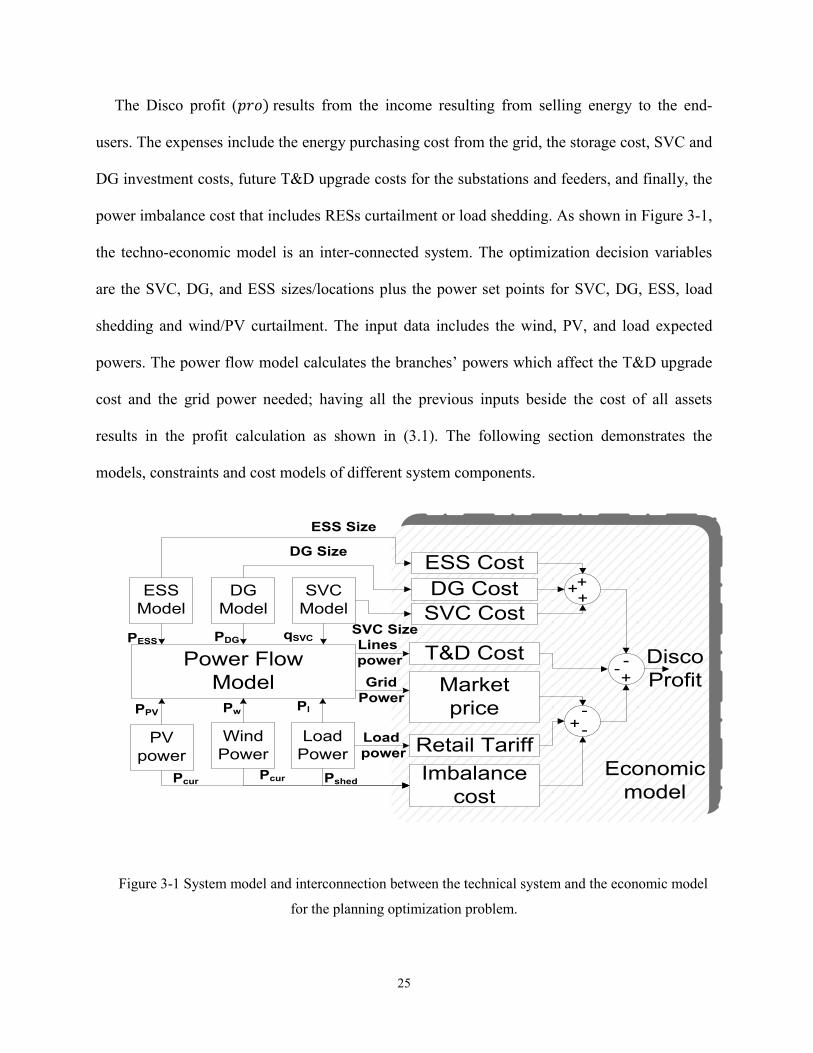
The Disco profit (𝑝𝑟𝑜) results from the income resulting from selling energy to the end-
users. The expenses include the energy purchasing cost from the grid, the storage cost, SVC and
DG investment costs, future T&D upgrade costs for the substations and feeders, and finally, the
power imbalance cost that includes RESs curtailment or load shedding. As shown in Figure 3-1,
the techno-economic model is an inter-connected system. The optimization decision variables
are the SVC, DG, and ESS sizes/locations plus the power set points for SVC, DG, ESS, load
shedding and wind/PV curtailment. The input data includes the wind, PV, and load expected
powers. The power flow model calculates the branches’ powers which affect the T&D upgrade
cost and the grid power needed; having all the previous inputs beside the cost of all assets
results in the profit calculation as shown in (3.1). The following section demonstrates the
models, constraints and cost models of different system components.
Power Flow
Model
ESS
Model
DG
Model
SVC
Model
PV
power
Wind
Power
Load
Power
ESS Cost
SVC Cost
DG Cost
T&D Cost
Retail Tariff
Market
price
Imbalance
costPcur
Pcur Pshed
ESS Size
DG Size
Lines
power
Grid
Power
Load
power
qSVCPDGPESS
PlPwPPV -+-
--
Disco
Profit
+++
+
SVC Size
Economic
model
Figure 3-1 System model and interconnection between the technical system and the economic model
for the planning optimization problem.

26
3.2.1 ESS Dynamic Model
At any sample t, the ESS is either charging power ch or discharging power dc. The ESS
power 𝑝𝐸𝑆 is the sum of these two powers as expressed in (3.2). The discharge power is
negative whereas the charge power is positive; both are limited by the ESS rated apparent
power 𝕊𝐸𝑆 as expressed in (3.2)-(3.4). The binary variable 𝑐𝑒𝑦,𝑠𝑐,𝑡𝐸𝑆 (𝑖) guarantees that the
discharge and charge powers are mutually exclusive at each sample time for each ESS. Further,
when charging is enabled 𝑐𝑒𝑦,𝑠𝑐,𝑡𝐸𝑆 (𝑖) = 1, the first constraints of (3.3), 0 ≤ 𝑐ℎ𝑦,𝑠𝑐,𝑡
𝐸𝑆 (𝑖) ≤ 𝕊𝐸𝑆(𝑖),
is dominant because 𝕊𝐸𝑆(𝑖) ≤ 𝕊𝐸𝑆 . When charging is disabled 𝑐𝑒𝑦,𝑠𝑐,𝑡𝐸𝑆 (𝑖) = 0, the second
constraint of (3.3) is dominant. A similar logic applies to the discharging constraint (3.4).
Decomposing the constraints in this way (instead of 0 ≤ 𝑐ℎ𝑦,𝑠𝑐,𝑡𝐸𝑆 (𝑖) ≤ 𝕊𝐸𝑆𝑐𝑒𝑦,𝑠𝑐,𝑡
𝐸𝑆 (𝑖)) enables the
inclusion of both the operational and planning constraints in a mixed-integer linear forms
instead of nonlinear ones.
𝑝𝑦,𝑠𝑐,𝑡𝐸𝑆 (𝑖) = 𝑐ℎ𝑦,𝑠𝑐,𝑡
𝐸𝑆 (𝑖) + 𝑑𝑐𝑦,𝑠𝑐,𝑡𝐸𝑆 (𝑖)
0 ≤ 𝑐ℎ𝑦,𝑠𝑐,𝑡𝐸𝑆 (𝑖) ≤ 𝕊𝐸𝑆(𝑖) 0 ≤ 𝑐ℎ𝑦,𝑠𝑐,𝑡
𝐸𝑆 (𝑖) ≤ 𝕊𝐸𝑆 𝑐𝑒𝑦,𝑠𝑐,𝑡𝐸𝑆 (𝑖)
−𝕊𝐸𝑆(𝑖) ≤ 𝑑𝑐𝑦,𝑠𝑐,𝑡𝐸𝑆 (𝑖) ≤ 0 −𝕊𝐸𝑆 (1 − 𝑐𝑒𝑦,𝑠𝑐,𝑡
𝐸𝑆 (𝑖)) ≤ 𝑑𝑐𝑦,𝑠𝑐,𝑡𝐸𝑆 (𝑖) ≤ 0
(3.2)
(3.3)
(3.4)
The ESS instantaneous energy 𝐸𝑦,𝑠𝑐,𝑡𝐸𝑆 is calculated dynamically from the ESS power whereas
both the charge and discharge efficiencies are considered as in (3.5) such that ( 𝜂𝑐ℎ < 1, 𝜂𝑑𝑐 >
1). The notation 𝜂𝑑𝑐represents the reciprocal of the per-unit discharge efficiency. It is worth
mentioning that an hourly sample rate is considered; thus the power equals the energy. The ESS
energy is limited by its rated capacity in (3.6). The number of cycles 𝑁𝐸𝑆 is another expression
used to count the absorbed and injected power from the ESS daily (in Watt-hours) as in (3.7).
When a rated capacity 𝔼𝐸𝑆is absorbed and injected by an ESS, 𝑁𝐸𝑆 is incremented by 1× 𝔼𝐸𝑆. 𝑁𝐸𝑆
27
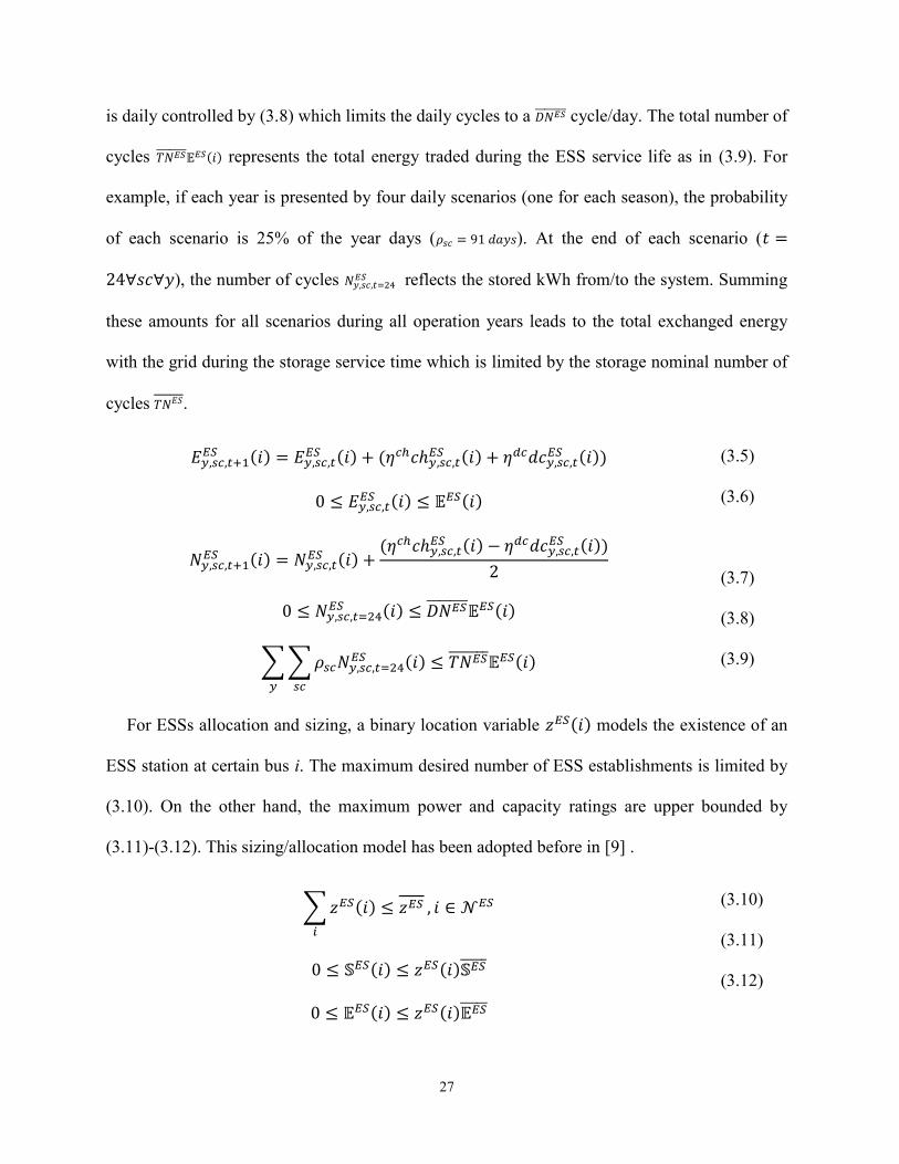
is daily controlled by (3.8) which limits the daily cycles to a 𝐷𝑁𝐸𝑆 cycle/day. The total number of
cycles 𝑇𝑁𝐸𝑆 𝔼𝐸𝑆(𝑖) represents the total energy traded during the ESS service life as in (3.9). For
example, if each year is presented by four daily scenarios (one for each season), the probability
of each scenario is 25% of the year days (𝜌𝑠𝑐 = 91 𝑑𝑎𝑦𝑠). At the end of each scenario (𝑡 =
24∀𝑠𝑐∀𝑦), the number of cycles 𝑁𝑦,𝑠𝑐,𝑡=24𝐸𝑆 reflects the stored kWh from/to the system. Summing
these amounts for all scenarios during all operation years leads to the total exchanged energy
with the grid during the storage service time which is limited by the storage nominal number of
cycles 𝑇𝑁𝐸𝑆 .
𝐸𝑦,𝑠𝑐,𝑡+1𝐸𝑆 (𝑖) = 𝐸𝑦,𝑠𝑐,𝑡
𝐸𝑆 (𝑖) + (𝜂𝑐ℎ𝑐ℎ𝑦,𝑠𝑐,𝑡𝐸𝑆 (𝑖) + 𝜂𝑑𝑐𝑑𝑐𝑦,𝑠𝑐,𝑡
𝐸𝑆 (𝑖))
0 ≤ 𝐸𝑦,𝑠𝑐,𝑡𝐸𝑆 (𝑖) ≤ 𝔼𝐸𝑆(𝑖)
𝑁𝑦,𝑠𝑐,𝑡+1𝐸𝑆 (𝑖) = 𝑁𝑦,𝑠𝑐,𝑡
𝐸𝑆 (𝑖) +(𝜂𝑐ℎ𝑐ℎ𝑦,𝑠𝑐,𝑡
𝐸𝑆 (𝑖) − 𝜂𝑑𝑐𝑑𝑐𝑦,𝑠𝑐,𝑡𝐸𝑆 (𝑖))
2
0 ≤ 𝑁𝑦,𝑠𝑐,𝑡=24𝐸𝑆 (𝑖) ≤ 𝐷𝑁𝐸𝑆 𝔼𝐸𝑆(𝑖)
∑∑𝜌𝑠𝑐𝑁𝑦,𝑠𝑐,𝑡=24𝐸𝑆 (𝑖)
𝑠𝑐𝑦
≤ 𝑇𝑁𝐸𝑆 𝔼𝐸𝑆(𝑖)
(3.5)
(3.6)
(3.7)
(3.8)
(3.9)
For ESSs allocation and sizing, a binary location variable 𝑧𝐸𝑆(𝑖) models the existence of an
ESS station at certain bus i. The maximum desired number of ESS establishments is limited by
(3.10). On the other hand, the maximum power and capacity ratings are upper bounded by
(3.11)-(3.12). This sizing/allocation model has been adopted before in [9] .
∑𝑧𝐸𝑆(𝑖) ≤ 𝑧𝐸𝑆
𝑖
, 𝑖 ∈ 𝒩𝐸𝑆
0 ≤ 𝕊𝐸𝑆(𝑖) ≤ 𝑧𝐸𝑆(𝑖)𝕊𝐸𝑆
0 ≤ 𝔼𝐸𝑆(𝑖) ≤ 𝑧𝐸𝑆(𝑖)𝔼𝐸𝑆
(3.10)
(3.11)
(3.12)
28
Because ESSs will participate in reactive power support in the proposed planning
framework, the reactive power is constrained by the power converter thermal capacity expressed
in (3.13). Because (3.13) is a nonlinear constraint (a sphere domain with a variable radius 𝕊𝐸𝑆),
it is linearized by a set of linear vectors 𝑓𝐸𝑆 that defines the ESS thermal capability domain
𝜑𝐸𝑆(𝑖) as explained in (3.14). Further details on the linearized domain are given in [9].
𝑝𝑦,𝑠𝑐,𝑡𝐸𝑆 (𝑖)2 + 𝑞𝑦,𝑠𝑐,𝑡
𝐸𝑆 (𝑖)2 ≤ 𝕊𝐸𝑆2
𝑓𝐸𝑆(𝑝𝑦,𝑠𝑐,𝑡𝐸𝑆 (𝑖), 𝑞𝑦,𝑠𝑐,𝑡
𝐸𝑆 (𝑖), 𝕊𝐸𝑆(𝑖)) ∈ 𝜑𝐸𝑆
(3.13)
(3.14)
The ESS initial capital cost in (3.15) includes its fixed cost 𝐹𝐶𝐸𝑆 (land, installation cost, etc.);
ESS power conversion system cost 𝐶𝐸𝑆
𝑀𝑊⁄ ; and ESS storage cost 𝐶𝐸𝑆
𝑀𝑊ℎ⁄ that stands for the
battery bank price. The operation and maintenance costs 𝑂&𝑀𝐸𝑆 are calculated and transferred
to the first year considering the interest rate 𝐼𝑅 during the project life y [9]; all operational future
costs are referred to the year of investment as a common time reference for a correct judgement
on the project cost/benefit analysis. If the inflation rate is significant, it can be included to
calculate the effective interest rate as explained in [23]. It is worth mentioning that the energy
constraint (3.6) allows a full battery discharge which may reduce its life time. As a
compensation, an extension for the ESS capacity can be added by setting 𝛼𝑇𝑁 (e.g., set 𝛼𝑇𝑁 = 0.2
for getting an equivalent life of 𝑇𝑁𝐸𝑆 at 20% minimum SOC).
𝑐𝐸𝑆 =∑𝑧𝐸𝑆(𝑖)𝐹𝐶𝐸𝑆(𝑖) + 𝐶𝐸𝑆
𝑀𝑉𝐴⁄ 𝕊𝐸𝑆(𝑖) + 𝐶
𝐸𝑆𝑀𝑊ℎ⁄ (1 + 𝛼𝑇𝑁)𝔼𝐸𝑆(𝑖) +
∑ ∑ 𝑧𝐸𝑆(𝑖)𝑂&𝑀𝐸𝑆(𝑖)𝑖𝑦
(1 + 𝐼𝑅)𝑌−1𝑖
(3.15)
3.2.2 Distributed Generation
Distributed generators (DGs), e.g., a micro turbine empowered by natural gas or a diesel
generator, are another possible investment option for T&D cost deferral. DGs power limit and
allocation are stated in (3.16)-(3.19). When a DG is connected to the grid via a voltage-source
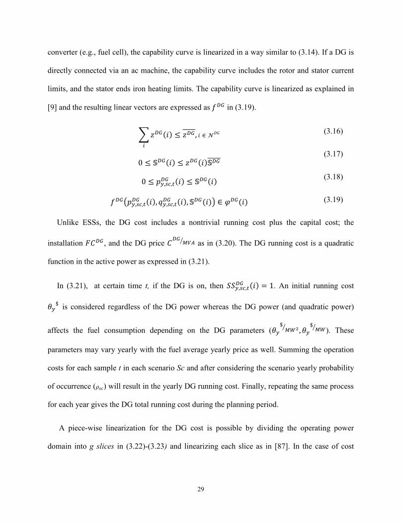
29
converter (e.g., fuel cell), the capability curve is linearized in a way similar to (3.14). If a DG is
directly connected via an ac machine, the capability curve includes the rotor and stator current
limits, and the stator ends iron heating limits. The capability curve is linearized as explained in
[9] and the resulting linear vectors are expressed as 𝑓𝐷𝐺 in (3.19).
∑𝑧𝐷𝐺(𝑖) ≤ 𝑧𝐷𝐺 , 𝑖 ∈ 𝒩𝐷𝐺
𝑖
0 ≤ 𝕊𝐷𝐺(𝑖) ≤ 𝑧𝐷𝐺(𝑖)𝕊𝐷𝐺
0 ≤ 𝑝𝑦,𝑠𝑐,𝑡𝐷𝐺 (𝑖) ≤ 𝕊𝐷𝐺(𝑖)
𝑓𝐷𝐺(𝑝𝑦,𝑠𝑐,𝑡𝐷𝐺 (𝑖), 𝑞𝑦,𝑠𝑐,𝑡
𝐷𝐺 (𝑖), 𝕊𝐷𝐺(𝑖)) ∈ 𝜑𝐷𝐺(𝑖)
(3.16)
(3.17)
(3.18)
(3.19)
Unlike ESSs, the DG cost includes a nontrivial running cost plus the capital cost; the
installation 𝐹𝐶𝐷𝐺 , and the DG price 𝐶𝐷𝐺
𝑀𝑉𝐴⁄ as in (3.20). The DG running cost is a quadratic
function in the active power as expressed in (3.21).
In (3.21), at certain time t, if the DG is on, then 𝑆𝑆𝑦,𝑠𝑐,𝑡𝐷𝐺 (𝑖) = 1. An initial running cost
𝜃𝑦$ is considered regardless of the DG power whereas the DG power (and quadratic power)
affects the fuel consumption depending on the DG parameters (𝜃𝑦$𝑀𝑊2⁄
, 𝜃𝑦$𝑀𝑊⁄
). These
parameters may vary yearly with the fuel average yearly price as well. Summing the operation
costs for each sample t in each scenario Sc and after considering the scenario yearly probability
of occurrence (𝜌𝑠𝑐) will result in the yearly DG running cost. Finally, repeating the same process
for each year gives the DG total running cost during the planning period.
A piece-wise linearization for the DG cost is possible by dividing the operating power
domain into g slices in (3.22)-(3.23) and linearizing each slice as in [87]. In the case of cost

30
linearization, the constraints in (3.23) are added to define the different linearization domains
limits.
𝑐𝐷𝐺 =∑𝑧𝐷𝐺(𝑖)𝐹𝐶𝐷𝐺(𝑖) + 𝐶𝐷𝐺
𝑀𝑉𝐴⁄ 𝕊𝐷𝐺(𝑖) +∑ ∑ 𝑧𝐷𝐺(𝑖)𝑂&𝑀𝐷𝐺(𝑖) + 𝑂𝐶𝑦
𝐷𝐺(𝑖)𝑖𝑦
(1 + 𝐼𝑅)𝑦−1𝑖
𝑂𝐶𝑦𝐷𝐺(𝑖) =∑∑𝜌𝑠𝑐∑𝜃𝑦
$𝑀𝑊2⁄
(𝑝𝑠𝑐,𝑦,𝑡𝐷𝐺 (𝑖))2
𝑡𝑠𝑐𝑦
+ 𝜃𝑦$𝑀𝑊⁄
𝑝𝑦,𝑠𝑐,𝑡𝐷𝐺 (𝑖) + 𝜃𝑦
$𝑆𝑆𝑦,𝑠𝑐,𝑡𝐷𝐺 (𝑖)
𝑂𝐶𝑦𝐷𝐺(𝑖) ≅∑∑𝜌𝑠𝑐∑∑ 𝛽𝑦
$𝑀𝑊⁄
𝑝𝑦,𝑠𝑐,𝑡𝐷𝐺𝑔 (𝑖) + 𝛽𝑦
$
𝑔𝑡𝑠𝑐𝑦
𝑆𝑆𝑦,𝑠𝑐,𝑡𝐷𝐺 (𝑖)
𝑝𝑠𝑐,𝑦,𝑡𝐷𝐺 (𝑖) =∑𝑝𝑦,𝑠𝑐,𝑡
𝐷𝐺𝑔 (𝑖)
𝑔
, 0 ≤ 𝑝𝑦,𝑠𝑐,𝑡𝐷𝐺𝑔 (𝑖) ≤ 𝑆𝑆𝑦,𝑠𝑐,𝑡
𝐷𝐺 (𝑖)𝑝𝐷𝐺𝑔
(3.20)
(3.21)
(3.22)
(3.23)
For a viable DG investment, the Levelized cost of its production ($/MWh) must be less than
the grid price; otherwise, the optimization process will not consider such investment as a cost-
saving one. In some cases, DGs are owned by the consumers, which became allowed by most of
the Discos. In such a case, the DG generation schedule is considered as an input for the power
flow model without including DGs as an investment option in the planning scheme. It is worth
mentioning that such a detailed model for the DG cost introduces many variables to the
planning problem; thus, it is practical to consider such a model with a few number of DGs.
When the number of DGs is large, modeling simplifications (such as considering a linear
operating cost and neglecting start-up cost) are acceptable for the sake of problem
simplification.
3.2.3 Static VAr Compensator (SVCs)
The SVCs can provide an efficient voltage regulation service by installing them at the far end
buses in case of weak grids. Improving the voltage profile reduces the power loss and increases

31
the feeder current carrying capacity. The allocation and rating of SVCs are governed by (3.24)-
(3.26) whereas the SVC cost (capital and O&M) is stated in (3.27).
∑𝑧𝑆𝑉𝐶(𝑖) ≤ 𝑧𝑆𝑉𝐶 , 𝑖 ∈ 𝒩𝑆𝑉𝐶
𝑖
0 ≤ ℚ𝑆𝑉𝐶(𝑖) ≤ 𝑧𝑆𝑉𝐶(𝑖)ℚ𝑆𝑉𝐶
−ℚ𝑆𝑉𝐶(𝑖) ≤ 𝑞𝑦,𝑠𝑐,𝑡𝑆𝑉𝐶 (𝑖) ≤ ℚ𝑆𝑉𝐶(𝑖)
𝑐𝑆𝑉𝐶 =∑𝑧𝑆𝑉𝐶(𝑖)𝐹𝐶𝑆𝑉𝐶(𝑖) + 𝐶𝑆𝑉𝐶
𝑀𝑉𝑅⁄ ℚ𝑆𝑉𝐶(𝑖) +∑ ∑ 𝑧𝑆𝑉𝐶(𝑖)𝑂&𝑀𝑆𝑉𝐶(𝑖)𝑖𝑦
(1 + 𝐼𝑅)𝑦−1𝑖
(3.24)
(3.25)
(3.26)
(3.27)
3.2.4 Power Imbalance Solutions
The power imbalance results from unexpected changes in loads or variations in the power
generated by RESs. The system operator can use many tools to rebalance the power, like load
shedding, RES curtailment, or up and down regulation by exporting/importing extra energy
from grid/ESS/DGs. The load shedding is constrained by each bus load power as in (3.28)
whereas the RES curtailment is limited by the RES power in (3.29). To avoid excessive load
shedding, the constraint in (3.30) keeps the disconnected load energy below a certain level 𝔼𝑠ℎ𝑑
that agrees with the power quality and reliability standards.
0 ≤ 𝑝𝑦,𝑠𝑐,𝑡𝑠ℎ𝑑 (𝑖) ≤ 𝑝𝑦,𝑠𝑐,𝑡
𝑙𝑜𝑎𝑑 (𝑖), 𝑖 ∈ 𝒩𝑙𝑜𝑎𝑑
0 ≤ 𝑝𝑦,𝑠𝑐,𝑡𝑐𝑢𝑟 (𝑖) ≤ 𝑝𝑦,𝑠𝑐,𝑡
𝑟𝑒𝑠 (𝑖), 𝑖 ∈ 𝒩𝑅𝐸𝑆
∑∑𝜌𝑠𝑐∑∑𝑝𝑦,𝑠𝑐,𝑡𝑠ℎ𝑑 (𝑖) ≤
𝑖𝑡𝑠𝑐𝑦
𝔼𝑠ℎ𝑑
(3.28)
(3.29)
(3.30)
The cost associated with load shedding 𝑐𝑠ℎ𝑑 in (3.31) represents a loss of energy sale priced
at 𝑠𝑝𝑠𝑐,𝑦,𝑡, plus a penalty 𝑠𝑝𝑒𝑛𝑠𝑐,𝑦,𝑡paid by the Disco to the consumer for the loss of service,
𝑠𝑝𝑒𝑛𝑠𝑐,𝑦,𝑡 is a time-variant penalty because the shedding time affects the customer comfort level

32
differently. Regarding the RES curtailment cost 𝑐𝑐𝑢𝑟, it may be modelled to include the levelized
generation cost of the RES plus an environmental penalty for curtailing a clean power source
(𝑐𝑝𝑒𝑛) as in (3.32).
𝑐𝑠ℎ𝑑 =∑∑𝜌𝑠𝑐∑(𝑠𝑝𝑦,𝑠𝑐,𝑡 + 𝑠𝑝𝑒𝑛𝑦,𝑠𝑐,𝑡)∑𝑝𝑦,𝑠𝑐,𝑡𝑠ℎ𝑑 (𝑖)
𝑖𝑡𝑠𝑐
𝑦
𝑐𝑐𝑢𝑟 =∑∑𝜌𝑠𝑐∑(𝑐𝑝𝑒𝑛)∑𝑝𝑦,𝑠𝑐,𝑡𝑐𝑢𝑟 (𝑖)
𝑖𝑡𝑠𝑐𝑦
(3.31)
(3.32)
Finally, the total power imbalance cost is defined as in (3.33).
𝑐𝑖𝑚𝑏 = 𝑐𝑐𝑢𝑟 + 𝑐𝑠ℎ𝑑 (3.33)
3.2.5 Power Flow Model
The power flow model for a radial distribution network consists of a single slack bus and a
set of PQ-buses 𝑖𝜖𝒩𝑏𝑢𝑠, 𝑖 ≠ 0 that connects a group of branches 𝑙: (𝑖 → 𝑗) ∈ 𝜓. In the power
flow model, the change in buses active and reactive power ∆𝑝𝑦,𝑠𝑐,𝑡𝑏𝑢𝑠 (𝑖), ∆𝑞𝑦,𝑠𝑐,𝑡
𝑏𝑢𝑠 (𝑖) leads to a
change in each node voltage amplitude and angle. For a set of buses 𝒩𝑏𝑢𝑠, the power is
represented as the sum of RESs (after curtailment), load (after shedding), DGs, SVC and ESS
powers as in (3.34)-(3.37). The injected power has a negative sign whereas the absorbed one is
positive. The ESS discharge power is negative as well. The loads are assumed as a constant
power type with a power factor 𝑝𝑓; thus the load reactive power is a constant ratio of the active
power as 𝑞𝑦,𝑠𝑐,𝑡𝐿𝑜𝑎𝑑 = 𝜆𝑦,𝑠𝑐,𝑡
𝑙𝑜𝑎𝑑 𝑝𝑦,𝑠𝑐,𝑡𝐿𝑜𝑎𝑑 , 𝜆𝑦,𝑠𝑐,𝑡
𝑙𝑜𝑎𝑑 = tan (cos−1 𝑝𝑓). Further, the RES reactive power can be
modeled by tuning 𝑞𝑠𝑐,𝑦,𝑡𝑟𝑒𝑠 but in such a case, an apparent power for RES has to be added.
𝑝𝑦,𝑠𝑐,𝑡𝑏𝑢𝑠 (𝑖) = (𝑝𝑦,𝑠𝑐,𝑡
𝐿𝑜𝑎𝑑(𝑖) − 𝑝𝑦,𝑠𝑐,𝑡𝑠ℎ𝑑 (𝑖)) − (𝑝𝑦,𝑠𝑐,𝑡
𝑟𝑒𝑠 (𝑖) − 𝑝𝑦,𝑠𝑐,𝑡𝑐𝑢𝑟 (𝑖)) − 𝑝𝑦,𝑠𝑐,𝑡
𝐷𝐺 (𝑖) + 𝑝𝑦,𝑠𝑐,𝑡𝐸𝑆 (𝑖)
𝑞𝑦,𝑠𝑐,𝑡𝑏𝑢𝑠 (𝑖) = (𝜆𝑦,𝑠𝑐,𝑡
𝑙𝑜𝑎𝑑 𝑝𝑦,𝑠𝑐,𝑡𝐿𝑜𝑎𝑑(𝑖) − 𝜆𝑦,𝑠𝑐,𝑡
𝑙𝑜𝑎𝑑 𝑝𝑦,𝑠𝑐,𝑡𝑠ℎ𝑑 (𝑖)) − 𝑞𝑦,𝑠𝑐,𝑡
𝑟𝑒𝑠 (𝑖) − 𝑞𝑦,𝑠𝑐,𝑡𝐷𝐺 (𝑖) + 𝑞𝑦,𝑠𝑐,𝑡
𝐸𝑆 (𝑖) − 𝑞𝑦,𝑠𝑐,𝑡𝑆𝑉𝐶 (𝑖)
∆𝑝𝑦,𝑠𝑐,𝑡𝑏𝑢𝑠 (𝑖) = −𝑝𝑦,𝑠𝑐,𝑡
𝑠ℎ𝑑 (𝑖) + 𝑝𝑦,𝑠𝑐,𝑡𝑐𝑢𝑟 (𝑖) − 𝑝𝑦,𝑠𝑐,𝑡
𝐷𝐺 (𝑖) + 𝑝𝑦,𝑠𝑐,𝑡𝐸𝑆 (𝑖)
(3.34)
(3.35)
(3.36)

33
∆𝑞𝑦,𝑠𝑐,𝑡𝑏𝑢𝑠 (𝑖) = −𝜆𝑦,𝑠𝑐,𝑡
𝑙𝑜𝑎𝑑 𝑝𝑦,𝑠𝑐,𝑡𝑠ℎ𝑑 (𝑖) − 𝑞𝑦,𝑠𝑐,𝑡
𝐷𝐺 (𝑖) + 𝑞𝑦,𝑠𝑐,𝑡𝐸𝑆 (𝑖) − 𝑞𝑦,𝑠𝑐,𝑡
𝑆𝑉𝐶 (𝑖) − 𝑞𝑦,𝑠𝑐,𝑡𝑟𝑒𝑠 (𝑖) (3.37)
In a distribution system with a low voltage-angle difference, many studies discussed the
power flow relaxation and convexification [88], [89]. One of the power flow approximations in
distribution systems uses the second-order cone programming as adopted before in [9] and [90].
Another simple linear technique depends on calculating the voltage Jacobian from the power
flow (voltage sensitivity to active and reactive power) [91]. The advantage of the sensitivity
technique is the resulting linear equality constraints that simplify the optimization problem,
especially with a huge number of variables and constraints, like the present planning problem.
The power loss sensitivity can be calculated as well [92], [93]. Before optimization, the initial
total power loss 𝑖𝑝𝑦,𝑠𝑐,𝑡𝑙𝑜𝑠𝑠 , 𝑖𝑞𝑦,𝑠𝑐,𝑡
𝑙𝑜𝑠𝑠 are calculated and the instantaneous loss sensitivity to the active
and reactive power matrices 𝑑𝑝𝑙𝑜𝑠𝑠
𝑑𝑃𝑏𝑢𝑠|𝑦,𝑠𝑐,𝑡
,𝑑𝑞𝑙𝑜𝑠𝑠
𝑑𝑃𝑏𝑢𝑠|𝑦,𝑠𝑐,𝑡
are obtained. The total power loss is
expressed as a sum of the initial power loss and the resulting losses due to any power change at
any bus as in (3.38)-(3.39). Finally, the grid power (slack bus) is the sum of all buses power
plus the total power loss [6] as shown in (3.40)-(3.41).
𝑝𝑦,𝑠𝑐,𝑡𝑙𝑜𝑠𝑠 = 𝑖𝑝𝑦,𝑠𝑐,𝑡
𝑙𝑜𝑠𝑠 +𝑑𝑝𝑙𝑜𝑠𝑠
𝑑𝑃𝑏𝑢𝑠|𝑦,𝑠𝑐,𝑡
∆𝑃𝑦,𝑠𝑐,𝑡𝑏𝑢𝑠 +
𝑑𝑝𝑙𝑜𝑠𝑠
𝑑𝑄𝑏𝑢𝑠|𝑦,𝑠𝑐,𝑡
∆𝑄𝑦,𝑠𝑐,𝑡𝑏𝑢𝑠
𝑞𝑦,𝑠𝑐,𝑡𝑙𝑜𝑠𝑠 = 𝑖𝑞𝑦,𝑠𝑐,𝑡
𝑙𝑜𝑠𝑠 +𝑑𝑞𝑙𝑜𝑠𝑠
𝑑𝑃𝑏𝑢𝑠|𝑦,𝑠𝑐,𝑡
∆𝑃𝑦,𝑠𝑐,𝑡𝑏𝑢𝑠 +
𝑑𝑞𝑙𝑜𝑠𝑠
𝑑𝑄𝑏𝑢𝑠|𝑦,𝑠𝑐,𝑡
∆𝑄𝑦,𝑠𝑐,𝑡𝑏𝑢𝑠
𝑝 𝑦,𝑠𝑐,𝑡𝑔𝑟𝑖𝑑
= 𝑝𝑦,𝑠𝑐,𝑡𝑏𝑢𝑠 (𝑖 = 0) = ∑ 𝑝𝑦,𝑠𝑐,𝑡
𝑏𝑢𝑠 (𝑖) + 𝑝𝑦,𝑠𝑐,𝑡𝑙𝑜𝑠𝑠
𝑖,𝑖≠0
𝑞 𝑦,𝑠𝑐,𝑡𝑔𝑟𝑖𝑑
= 𝑞𝑦,𝑠𝑐,𝑡𝑏𝑢𝑠 (𝑖 = 0) = ∑ 𝑞𝑦,𝑠𝑐,𝑡
𝑏𝑢𝑠 (𝑖) + 𝑞𝑦,𝑠𝑐,𝑡𝑙𝑜𝑠𝑠
𝑖,𝑖≠0
(3.38)
(3.39)
(3.40)
(3.41)
Because the total power loss is represented in the grid power expression, the branches power
is calculated by the power balance expression in (3.42)-(3.43) which indicates that the branch
power equals the branch output bus power plus the power transferred to other branches

34
connected to it [90]. The branch capacity is limited by (3.45), where the apparent power of the
feeder 𝑠 𝑠𝑐,𝑦,𝑡𝑓
(𝑙) is limited by the nominal feeder thermal capacity 𝕊𝑓(𝑙) after considering a
reserve capacity fr to account for uncertainties. A feeder extension is possible by adding a
capacity extension 𝕔𝑓𝑚 that is associated with the feeder upgrade method m; each method has a
different capacity extension that is enabled by the variable 𝑧𝑓𝑚(𝑙).
A linearized version of the constraint (3.45) is given in (3.46). It is worth mentioning that
linearizing (3.44) leads to convexifying the optimization problem at the price of adding more
variables and less accuracy for the capability function. For instance, Figure 3-2 compares the
constraint domain of the original capability curve (circle as in (3.44)); when this nonlinear
function is linearized around more operating points (twenty instead of eight for example), the
linearized constraints almost coincide with the circle. However, the number of constraints
increases from eight into twenty. As a result, this trade-off should be considered when
linearizing any nonlinear function. A similar concept applies to the constraints (3.14), (3.19).
𝑝𝑦,𝑠𝑐,𝑡𝑓 (𝑙) = 𝑝𝑦,𝑠𝑐,𝑡
𝑏𝑢𝑠 (𝑗) + ∑ 𝑝𝑦,𝑠𝑐,𝑡𝑓 (𝑘)
𝑘:(𝑗→𝑛)∈𝜓
, 𝑙: (𝑖 → 𝑗)
𝑞𝑦,𝑠𝑐,𝑡𝑓 (𝑙) = 𝑞𝑦,𝑠𝑐,𝑡
𝑏𝑢𝑠 (𝑗) + ∑ 𝑞𝑦,𝑠𝑐,𝑡𝑓 (𝑘)
𝑘:(𝑗→𝑛)∈𝜓
, 𝑙: (𝑖 → 𝑗)
𝑠 𝑦,𝑠𝑐,𝑡𝑓 2
(𝑙) = 𝑝 𝑦,𝑠𝑐,𝑡𝑓 2
(𝑙) + 𝑞 𝑦,𝑠𝑐,𝑡𝑓 2
(𝑙), 𝑙: (𝑖 → 𝑗)
‖𝑠 𝑦,𝑠𝑐,𝑡𝑓 (𝑙)‖ ≤ 𝕊𝑓(𝑙) +∑ 𝑧𝑓𝑚(𝑙)𝕔𝑓𝑚
𝑚(1 + 𝑓𝑟𝑓)⁄
𝑓𝑙(𝑝 𝑦,𝑠𝑐,𝑡𝑓 (𝑙), 𝑞 𝑦,𝑠𝑐,𝑡
𝑓 (𝑙)) ≤ 𝕊𝑓(𝑙) +∑ 𝑧𝑓𝑚(𝑙)𝕔𝑓𝑚𝑚
(1 + 𝑓𝑟𝑓)⁄
(3.42)
(3.43)
(3.44)
(3.45)
(3.46)
Regarding the voltage level, the initial voltage 𝑖𝑣𝑠𝑐,𝑦,𝑡 is first calculated before optimization.
After calculating the voltage sensitivity 𝑑𝑣(𝑖)
𝑑𝑃𝑏𝑢𝑠|𝑦,𝑠𝑐,𝑡
,𝑑𝑣(𝑖)
𝑑𝑄𝑏𝑢𝑠|𝑦,𝑠𝑐,𝑡
, the nodal voltage magnitude is
given and limited in (3.47)-(3.48) as a function of the buses power change. Finally, the Disco
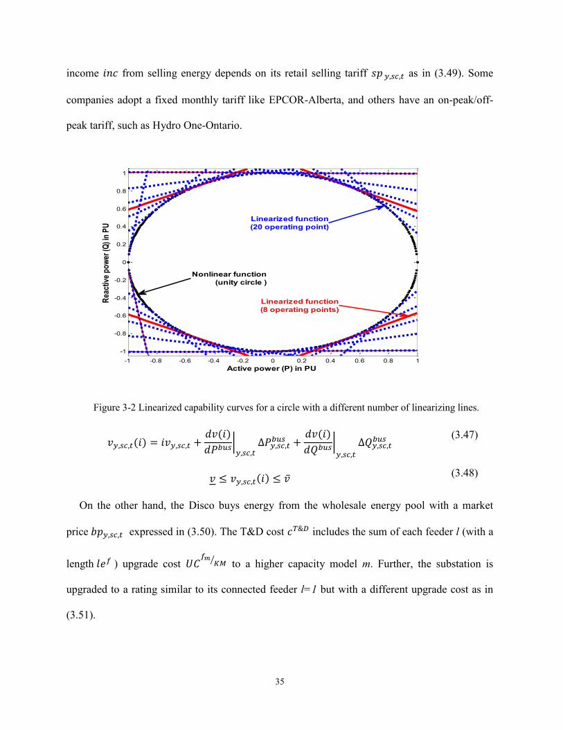
35
income 𝑖𝑛𝑐 from selling energy depends on its retail selling tariff 𝑠𝑝 𝑦,𝑠𝑐,𝑡 as in (3.49). Some
companies adopt a fixed monthly tariff like EPCOR-Alberta, and others have an on-peak/off-
peak tariff, such as Hydro One-Ontario.
Figure 3-2 Linearized capability curves for a circle with a different number of linearizing lines.
𝑣𝑦,𝑠𝑐,𝑡(𝑖) = 𝑖𝑣𝑦,𝑠𝑐,𝑡 +𝑑𝑣(𝑖)
𝑑𝑃𝑏𝑢𝑠|𝑦,𝑠𝑐,𝑡
∆𝑃𝑦,𝑠𝑐,𝑡𝑏𝑢𝑠 +
𝑑𝑣(𝑖)
𝑑𝑄𝑏𝑢𝑠|𝑦,𝑠𝑐,𝑡
∆𝑄𝑦,𝑠𝑐,𝑡𝑏𝑢𝑠
𝑣 ≤ 𝑣𝑦,𝑠𝑐,𝑡(𝑖) ≤ ��
(3.47)
(3.48)
On the other hand, the Disco buys energy from the wholesale energy pool with a market
price 𝑏𝑝𝑦,𝑠𝑐,𝑡 expressed in (3.50). The T&D cost 𝑐𝑇&𝐷 includes the sum of each feeder l (with a
length 𝑙𝑒𝑓 ) upgrade cost 𝑈𝐶𝑓𝑚
𝐾𝑀⁄ to a higher capacity model m. Further, the substation is
upgraded to a rating similar to its connected feeder l=1 but with a different upgrade cost as in
(3.51).
-1 -0.8 -0.6 -0.4 -0.2 0 0.2 0.4 0.6 0.8 1
-1
-0.8
-0.6
-0.4
-0.2
0
0.2
0.4
0.6
0.8
1
Active power (P) in PU
Rea
ctiv
e p
ow
er (Q
) in
PU
Linearized function
(8 operating points)
Linearized function
(20 operating point)
Nonlinear function
(unity circle )
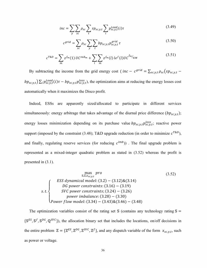
36
𝑖𝑛𝑐 =∑∑𝜌𝑠𝑐∑𝑠𝑝𝑠𝑐,𝑦,𝑡∑𝑝𝑠𝑐,𝑦,𝑡𝐿𝑜𝑎𝑑(𝑖)𝜏
𝑖𝑡𝑠𝑐𝑦
𝑐𝑔𝑟𝑖𝑑 =∑𝜌𝑠𝑐∑∑𝑏𝑝𝑠𝑐,𝑦,𝑡𝑝𝑠𝑐,𝑦,𝑡𝑔𝑟𝑖𝑑
𝑡𝑦𝑠𝑐
𝜏
𝑐𝑇&𝐷 =∑𝑧𝑓𝑚(1)
𝑚
𝑈𝐶𝑠𝑢𝑏𝑚 +∑∑𝑧𝑓𝑚(𝑙)
𝑚
𝑙𝑒𝑓(𝑙)𝑈𝐶𝑓𝑚
𝐾𝑀⁄
𝑙
(3.49)
(3.50)
(3.51)
By subtracting the income from the grid energy cost ( 𝑖𝑛𝑐 − 𝑐𝑔𝑟𝑖𝑑 = ∑ 𝜌𝑠𝑐(𝑠𝑝𝑠𝑐,𝑦,𝑡 −𝑠𝑐,𝑦,𝑡
𝑏𝑝𝑠𝑐,𝑦,𝑡)∑ 𝑝𝑠𝑐,𝑦,𝑡𝐿𝑜𝑎𝑑(𝑖)𝜏𝑖 − 𝑏𝑝𝑠𝑐,𝑦,𝑡𝑝𝑠𝑐,𝑦,𝑡
𝑙𝑜𝑠𝑠 ), the optimization aims at reducing the energy losses cost
automatically when it maximizes the Disco profit.
Indeed, ESSs are apparently sized/allocated to participate in different services
simultaneously: energy arbitrage that takes advantage of the diurnal price difference (𝑏𝑝𝑠𝑐,𝑦,𝑡);
energy losses minimization depending on its purchase value 𝑏𝑝𝑠𝑐,𝑦,𝑡𝑝𝑠𝑐,𝑦,𝑡𝑙𝑜𝑠𝑠 ; reactive power
support (imposed by the constraint (3.48); T&D upgrade reduction (in order to minimize 𝑐𝑇&𝐷),
and finally, regulating reserve services (for reducing 𝑐𝑖𝑚𝑏)) . The final upgrade problem is
represented as a mixed-integer quadratic problem as stated in (3.52) whereas the profit is
presented in (3.1).
max𝕊,ℤ,𝑥𝑠𝑐,𝑦,𝑡
𝑝𝑟𝑜
𝑠. 𝑡.
{
𝐸𝑆𝑆 𝑑𝑦𝑛𝑎𝑚𝑖𝑐𝑎𝑙 𝑚𝑜𝑑𝑒𝑙: (3.2) − (3.12)&(3.14)
𝐷𝐺 𝑝𝑜𝑤𝑒𝑟 𝑐𝑜𝑛𝑠𝑡𝑟𝑎𝑖𝑛𝑡𝑠: (3.16) − (3.19)
𝑆𝑉𝐶 𝑝𝑜𝑤𝑒𝑟 𝑐𝑜𝑛𝑠𝑡𝑟𝑎𝑖𝑛𝑡𝑠; (3.24) − (3.26)
𝑝𝑜𝑤𝑒𝑟 𝑖𝑚𝑏𝑎𝑙𝑎𝑛𝑐𝑒: (3.28) − (3.30)
𝑃𝑜𝑤𝑒𝑟 𝑓𝑙𝑜𝑤 𝑚𝑜𝑑𝑒𝑙: (3.34) − (3.43)&(3.46) − (3.48)
(3.52)
The optimization variables consist of the rating set 𝕊 (contains any technology rating 𝕊 =
{𝕊𝐸𝑆, 𝕊𝑓 , 𝕊𝐷𝐺 , ℚ𝑆𝑉𝐶}), the allocation binary set that includes the locations, on/off decisions in
the entire problem ℤ = {ℤ𝐸𝑆, ℤ𝐷𝐺 , ℤ𝑆𝑉𝐶 , ℤ𝑓}, and any dispatch variable of the form 𝑥𝑠𝑐,𝑦,𝑡, such
as power or voltage.

37
For each year y, the daily scenario changes from season to season, from month to month and
even from working days to weekends (e.g., as depicted in Figure 3-5 for the first-year daily
scenarios).
Considering 365 daily scenarios per year or even more than 365 by assuming an 𝑘 possibility
for each daily scenario such that ∑ ∑ ∑ 𝜌𝑘,𝑠𝑐𝑘𝑠𝑐 = 1𝑦 , the previous assumptions will lead to an
enormous problem size. As a result, and without loss of generalization, this work uses a
scenarios minimizations technique using the k-means method similar to the one adopted in [9].
First, each day 𝑛 is represented by a realization 𝑅𝑒𝑛that consists of PV, load, wind and price
normalized data where (𝑅𝑒𝑛, 𝑛 = 1:𝓃 dimension is 1×96 in case of hourly sampled data. By
setting the number of desired scenarios to J, the k-means clustering approximates all the 𝓃
realizations by a 𝐽 centroids (𝒸𝑠𝑐 , 𝑠𝑐 = 1: 𝐽). The Euclidian distance of each realization is
𝑑𝑁𝑠𝑐 = ‖𝑅𝑒𝑁 − 𝒸𝑠𝑐‖2 defines the belonging factor (the membership value) of each realization
𝑅𝑒𝑁 to a certain centroid 𝒸𝐽. Finally, 𝑑𝑁𝑠𝑐 is used to calculate the probability of each
centroid 𝜌𝑠𝑐
.
Regarding the quality of this approximation, Figure 3-4 shows the per unit (pu) Euclidean
distance of each realization of the first year (shown in Figure 3-5) with the ten approximating
scenarios. The sum of all distances from a realization to all scenarios is equal to one. Although
four scenarios (1, 4, 6, and 9) can approximate the realizations accurately because they are very
close to most of the scenarios (their mean pu distance to all realization is less than 0.05 pu and
consequently they have a higher probability 𝜌𝑠𝑐
), these scenarios, still, have a long distance to
some special realizations (e.g., days with an unusual load profile or volatile market). Such
uncommon realizations are well fitted by the other scenarios that have a very close distance to
them while they are far away from most of common realizations.
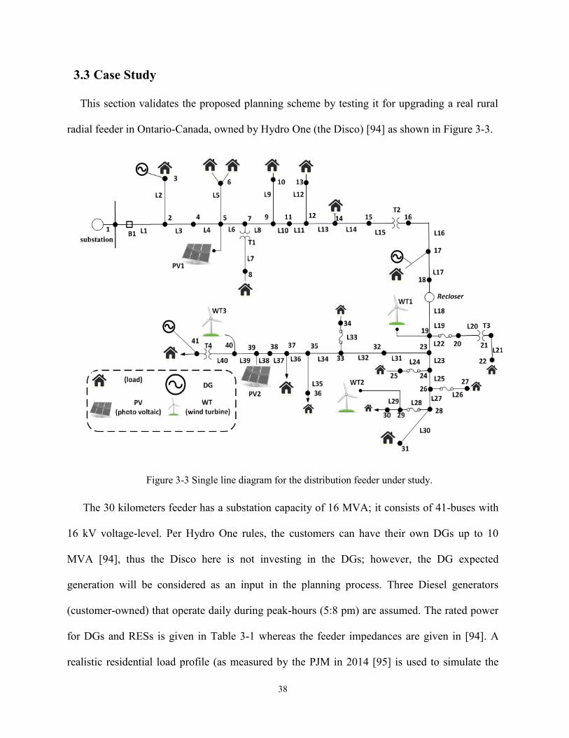
38
3.3 Case Study
This section validates the proposed planning scheme by testing it for upgrading a real rural
radial feeder in Ontario-Canada, owned by Hydro One (the Disco) [94] as shown in Figure 3-3.
Figure 3-3 Single line diagram for the distribution feeder under study.
The 30 kilometers feeder has a substation capacity of 16 MVA; it consists of 41-buses with
16 kV voltage-level. Per Hydro One rules, the customers can have their own DGs up to 10
MVA [94], thus the Disco here is not investing in the DGs; however, the DG expected
generation will be considered as an input in the planning process. Three Diesel generators
(customer-owned) that operate daily during peak-hours (5:8 pm) are assumed. The rated power
for DGs and RESs is given in Table 3-1 whereas the feeder impedances are given in [94]. A
realistic residential load profile (as measured by the PJM in 2014 [95] is used to simulate the

39
load as depicted in Figure 3-5-a; each season has a unique load profile with higher peak during
summer. A 4% yearly load growth is assumed during this study; thus, the nominal load is
expected to reach 22.77 MVA in ten years. Two PV plants are added to the system with a real
PV radiation taken from [96], shown in Figure 3-5-b with longer generation hours during
summer that reduce gradually while moving toward winter. The PV generation is assumed to
have the same growth rate as the load [9] whereas the wind generation capacity is fixed. Three
wind facilities are dispersed on the feeder to make the total RES penetration of this feeder 37%
calculated as a ratio between the maximum RES output to peak load. A real wind generation is
considered [97] as depicted in Figure 3-5-d. It is worth mentioning that winter days are windier
than summer days, especially during late night hours. The buy price of Ontario (HOEP: hourly
Ontario Energy Price) is provided by the Independent Electricity System Operator (IESO) in
[98] and depicted in Figure 3-5-c. It is very important to notice that some days have a very high
price difference which indicates that energy arbitrage will be a successful investment in such a
market.
It is assumed that the Disco considers an energy billing price 20% more than the HOEP
average price. Due to the enormous problem size and number of states, the yearly realizations
are minimized to ten scenarios per year; this results in a total hundred scenarios for the whole
planning horizon. The wind generation curtailment is penalized by 100$/MWh and load
shedding by 150$/MWh with maximum 30-minute load shedding period/year. These high
values are chosen by trial and error to avoid over-curtailment and over-load shedding during the
optimization process; otherwise these options, which remarkably affect the system reliability in
a negative way, would be preferred by the optimization algorithm than the upgrade ones.
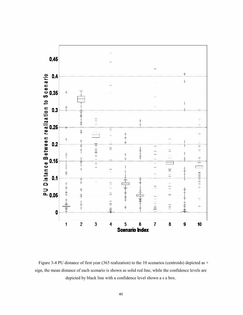
40
Figure 3-4 PU distance of first year (365 realization) to the 10 scenarios (centroids) depicted as +
sign, the mean distance of each scenario is shown as solid red line, while the confidence levels are
depicted by black line with a confidence level shown a s a box.
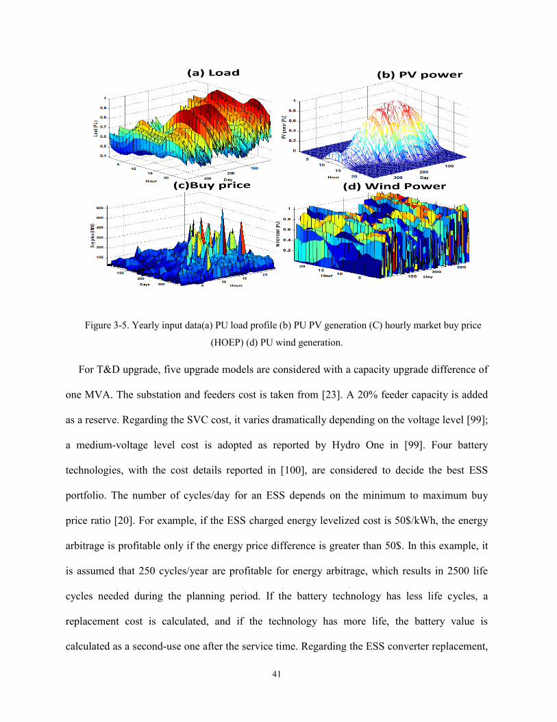
41
Figure 3-5. Yearly input data(a) PU load profile (b) PU PV generation (C) hourly market buy price
(HOEP) (d) PU wind generation.
For T&D upgrade, five upgrade models are considered with a capacity upgrade difference of
one MVA. The substation and feeders cost is taken from [23]. A 20% feeder capacity is added
as a reserve. Regarding the SVC cost, it varies dramatically depending on the voltage level [99];
a medium-voltage level cost is adopted as reported by Hydro One in [99]. Four battery
technologies, with the cost details reported in [100], are considered to decide the best ESS
portfolio. The number of cycles/day for an ESS depends on the minimum to maximum buy
price ratio [20]. For example, if the ESS charged energy levelized cost is 50$/kWh, the energy
arbitrage is profitable only if the energy price difference is greater than 50$. In this example, it
is assumed that 250 cycles/year are profitable for energy arbitrage, which results in 2500 life
cycles needed during the planning period. If the battery technology has less life cycles, a
replacement cost is calculated, and if the technology has more life, the battery value is
calculated as a second-use one after the service time. Regarding the ESS converter replacement,

42
a DC-AC converter has a long lifetime that may reach 12 years [101] due to switches low
failure rate and the use of reliable film capacitors. As a result, no ESS converter replacement
cost is considered in this 10 years planning project.
It is also possible to just define the maximum number of cycles during the planning period
without imposing a daily number of cycles (by omitting constraint (3.8)). In such a case, the
optimization decides the optimal daily number of cycles according to the market profile.
Further, the total number of cycles constraint may be omitted as well; however, a life cycle
dependent ESS cost model should be considered in the objective function [20] (nonconvex
optimization needed). One may argue that ten years’ market predictions are not that accurate;
thus, it is safer to assume a maximum one daily number of cycles and the total life cycles
instead of possible ESS oversizing that may result from misleading long-horizon predictions. In
both cases, it is the designer choice according to their philosophy (optimistic or conservative)
and their trust of provided predictions.
As a general case, all buses are considered as candidates for ESSs and SVCs (𝒩𝐸𝑆 = 𝒩𝑆𝑉𝐶 =
𝒩𝑏𝑢𝑠). However, in this study, ten buses along the feeders are chosen as candidates for ESSs and
SVCs as shown in Table 3-1.
Table 3-1 Planning input data.
RES, DG rating 𝑝𝑤𝑡1 = 2𝑀𝑊, 𝑝𝑤𝑡2 = 𝑝𝑤𝑡3 = 1.5𝑀𝑊, 𝑝𝐷𝐺1 = 1 𝑀𝑊
𝑝𝑝𝑣1 = 𝑝𝑝𝑣2 = 0.5 𝑀𝑊, 𝑝𝐷𝐺2 = 𝑝𝐷𝐺3 = 0.5 𝑀𝑊
ESS Lead-Acid Na-
S
Zn-
Br
Li-
ion
𝐶𝐸𝑆
𝑀𝑉𝐴⁄ $/ MVA installed 400 350 400 400
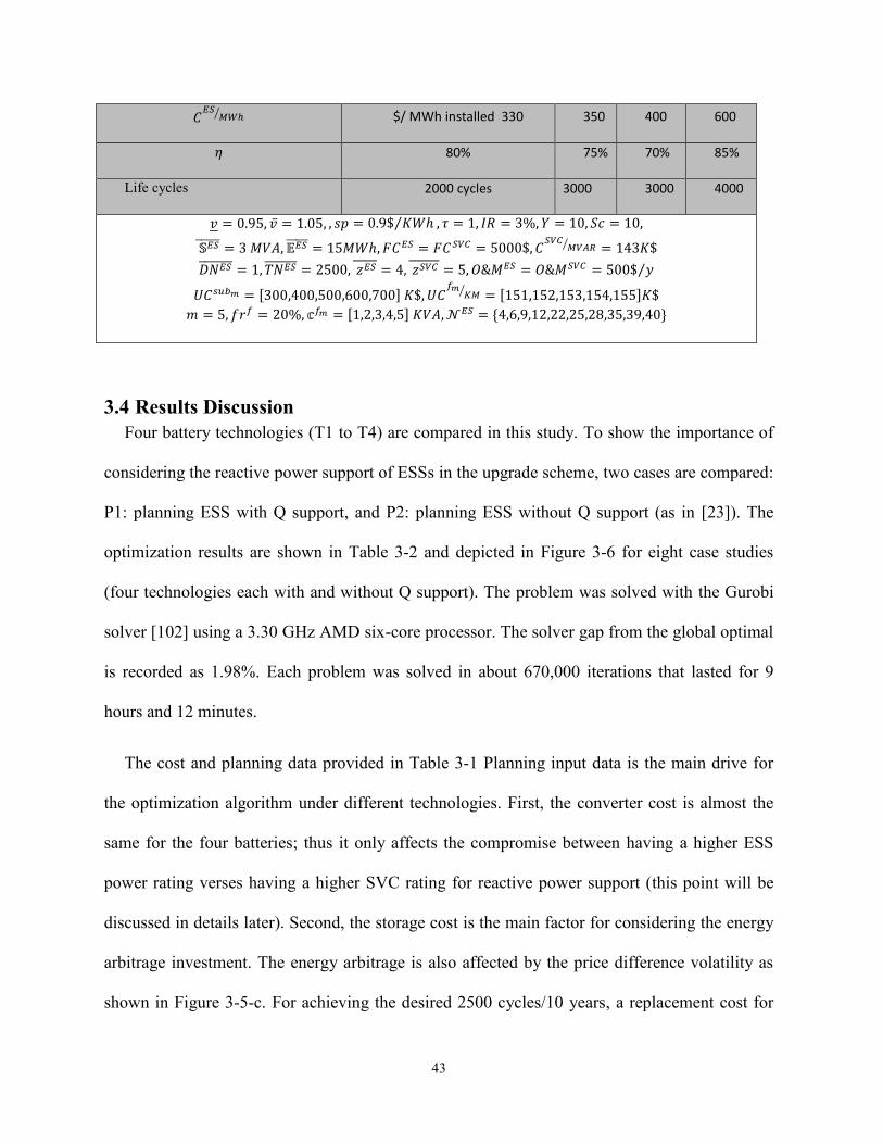
43
𝐶𝐸𝑆
𝑀𝑊ℎ⁄ $/ MWh installed 330 350 400 600
𝜂 80% 75% 70% 85%
Life cycles 2000 cycles 3000 3000 4000
𝑣 = 0.95, �� = 1.05, , 𝑠𝑝 = 0.9$ 𝐾𝑊ℎ⁄ , 𝜏 = 1, 𝐼𝑅 = 3%, 𝑌 = 10, 𝑆𝑐 = 10,
𝕊𝐸𝑆 = 3 𝑀𝑉𝐴, 𝔼𝐸𝑆 = 15𝑀𝑊ℎ, 𝐹𝐶𝐸𝑆 = 𝐹𝐶𝑆𝑉𝐶 = 5000$, 𝐶𝑆𝑉𝐶
𝑀𝑉𝐴𝑅⁄ = 143𝐾$
𝐷𝑁𝐸𝑆 = 1, 𝑇𝑁𝐸𝑆 = 2500, 𝑧𝐸𝑆 = 4, 𝑧𝑆𝑉𝐶 = 5, 𝑂&𝑀𝐸𝑆 = 𝑂&𝑀𝑆𝑉𝐶 = 500$ 𝑦⁄
𝑈𝐶𝑠𝑢𝑏𝑚 = [300,400,500,600,700] 𝐾$, 𝑈𝐶𝑓𝑚
𝐾𝑀⁄ = [151,152,153,154,155]𝐾$
𝑚 = 5, 𝑓𝑟𝑓 = 20%, 𝕔𝑓𝑚 = [1,2,3,4,5] 𝐾𝑉𝐴,𝒩𝐸𝑆 = {4,6,9,12,22,25,28,35,39,40}
3.4 Results Discussion
Four battery technologies (T1 to T4) are compared in this study. To show the importance of
considering the reactive power support of ESSs in the upgrade scheme, two cases are compared:
P1: planning ESS with Q support, and P2: planning ESS without Q support (as in [23]). The
optimization results are shown in Table 3-2 and depicted in Figure 3-6 for eight case studies
(four technologies each with and without Q support). The problem was solved with the Gurobi
solver [102] using a 3.30 GHz AMD six-core processor. The solver gap from the global optimal
is recorded as 1.98%. Each problem was solved in about 670,000 iterations that lasted for 9
hours and 12 minutes.
The cost and planning data provided in Table 3-1 Planning input data is the main drive for
the optimization algorithm under different technologies. First, the converter cost is almost the
same for the four batteries; thus it only affects the compromise between having a higher ESS
power rating verses having a higher SVC rating for reactive power support (this point will be
discussed in details later). Second, the storage cost is the main factor for considering the energy
arbitrage investment. The energy arbitrage is also affected by the price difference volatility as
shown in Figure 3-5-c. For achieving the desired 2500 cycles/10 years, a replacement cost for
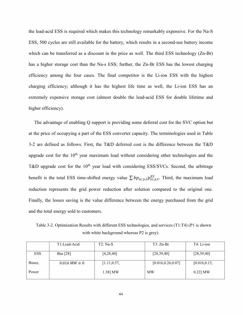
44
the lead-acid ESS is required which makes this technology remarkably expensive. For the Na-S
ESS, 500 cycles are still available for the battery, which results in a second-use battery income
which can be transferred as a discount in the price as well. The third ESS technology (Zn-Br)
has a higher storage cost than the Na-s ESS; further, the Zn-Br ESS has the lowest charging
efficiency among the four cases. The final competitor is the Li-ion ESS with the highest
charging efficiency; although it has the highest life time as well, the Li-ion ESS has an
extremely expensive storage cost (almost double the lead-acid ESS for double lifetime and
higher efficiency).
The advantage of enabling Q support is providing some deferral cost for the SVC option but
at the price of occupying a part of the ESS converter capacity. The terminologies used in Table
3-2 are defined as follows. First, the T&D deferred cost is the difference between the T&D
upgrade cost for the 10th year maximum load without considering other technologies and the
T&D upgrade cost for the 10th year load with considering ESS/SVCs. Second, the arbitrage
benefit is the total ESS time-shifted energy value ∑𝑏𝑝𝑠𝑐,𝑦,𝑡𝑝𝑠𝑐,𝑦,𝑡𝐸𝑆 . Third, the maximum load
reduction represents the grid power reduction after solution compared to the original one.
Finally, the losses saving is the value difference between the energy purchased from the grid
and the total energy sold to customers.
Table 3-2. Optimization Results with different ESS technologies, and services (T1:T4) (P1 is shown
with white background whereas P2 is grey).
T1:Lead-Acid T2: Na-S T3: Zn-Br T4: Li-ion
ESS
Buses,
Power
Bus [28] [4,28,40] [28,39,40] [28,39,40]
0.016 MW ≅ 0
[1.11,0.57,
1.38] MW
[0.016,0.26,0.07]
MW
[0.016,0.15,
0.22] MW
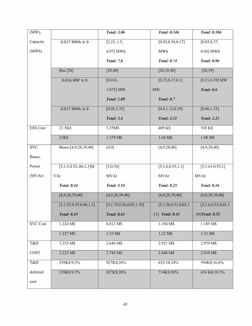
45
(MW),
Capacity
(MWh)
Total: 3.06 Total: 0.346 Total: 0.386
0.017 MWh ≅ 0 [2.23, 1.5,
4.07] MWh
Total: 7.8
[0.03,0.54,0.17]
MWh
Total: 0.74
[0.03,0.37,
0.56] MWh
Total: 0.96
Bus [28] [28,40] [28,39,40] [28,39]
0.016 MW ≅ 0 [0.016,
1.075] MW
Total: 1.09
[0.23,0.37,0.1]
MW
Total: 0.7
[0.21,0.39] MW
Total: 0.6
0.017 MWh ≅ 0 [0.05,3.35]
Total: 3.4
[0.8,1.12,0.29]
Total: 2.21
[0.86,1.35]
Total: 2.21
ESS Cost 21.5K$ 3.35M$ 409 K$ 538 K$
21K$ 1.379 M$ 1.04 M$ 1.08 M$
SVC
Buses,
Power
(MVAr)
Buses:[4,9,28,39,40] [4,9]
[4,9,28,40]
[4,9,28,40]
[5,1.5,0.53,.06,1.3]M
VAr
Total: 8.44
[5,0.54]
MVAr
Total: 5.54
[5,1.6,0.55,1.1]
MVAr
Total: 8.25
[5,1.61,0.55,1]
MVAr
Total: 8.16
[4,9,28,39,40] [4,9,28,39,40] [4,9,28,39,40] [4,9,28,39,40]
[5,1.52,0.55,0.06,1.3]
Total: 8.45
[5,1.75,0.56,0.03,1.29]
Total: 8.63
[5,1.58,0.51,0.01,1
.31] Total: 8.41
[5,1.6,0.55,0.01,1
.36]Total: 8.52
SVC Cost 1.224 M$ 0.812 M$ 1.194 M$ 1.185 M$
1.227 M$ 1.25 M$ 1.22 M$ 1.33 M$
T&D
COST
3.233 M$ 2.646 M$ 2.921 M$ 2.979 M$
3.233 M$ 2.745 M$ 2.848 M$ 2.919 M$
T&D
deferred
cost
339K$/9.5% 927K$/26% 652/18.24% 594K$/16.6%
339K$/9.5% 827K$/20% 714KS/20% 654 K$/18.3%
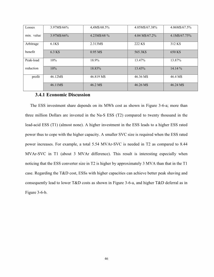
46
Losses
min. value
3.97M$/66% 4,4M$/68.5% 4.05M$/67.38% 4.06M$/67.5%
3.97M$/66% 4.23M$/68 % 4.04 M$/67.2% 4.1M$/67.75%
Arbitrage
benefit
6.1K$ 2.313M$ 222 K$ 312 K$
6.3 K$ 0.95 M$ 565.3K$ 650 K$
Peak-load
reduction
10% 18.9% 13.47% 13.87%
10% 18.83% 13.43% 14.14 %
profit 46.12M$ 46.819 M$ 46.36 M$ 46.4 M$
46.11M$ 46.2 M$ 46.26 M$ 46.24 M$
3.4.1 Economic Discussion
The ESS investment share depends on its MWh cost as shown in Figure 3-6-a; more than
three million Dollars are invested in the Na-S ESS (T2) compared to twenty thousand in the
lead-acid ESS (T1) (almost none). A higher investment in the ESS leads to a higher ESS rated
power thus to cope with the higher capacity. A smaller SVC size is required when the ESS rated
power increases. For example, a total 5.54 MVAr-SVC is needed in T2 as compared to 8.44
MVAr-SVC in T1 (about 3 MVAr difference). This result is interesting especially when
noticing that the ESS converter size in T2 is higher by approximately 3 MVA than that in the T1
case. Regarding the T&D cost, ESSs with higher capacities can achieve better peak shaving and
consequently lead to lower T&D costs as shown in Figure 3-6-a, and higher T&D deferral as in
Figure 3-6-b.

47
Figure 3-6 Sizing results for different ESS technologies in case of P1 (Q support) (a) different
technologies cost share (b) different incomes from the investment.
Regarding the power loss saving, a non-significant difference is noticed between ESS
technologies. In fact, the power loss minimization is dependent on the voltage profile. Because
the voltage deviations are kept within ∓5% in all cases, the power loss savings with different
ESS technologies are very close. On the other hand, the energy arbitrage income depends on the
ESS capacity (MWh); whereas T2 has 7 MWh more capacity (more or less) compared to other

48
technologies, T2 harvests two million Dollars extra income from energy arbitrage (shown in
Figure 3-6-b).
The T&D upgrade should not convey a profit in the first place; this is the case with T1 (lead-
acid) where the total cost exceeds the income. This means that the Disco will pay a part of their
energy trading profit (𝑖𝑛𝑐 − 𝑐𝑔𝑟𝑖𝑑) to cover the T&D upgrade costs. This is not the case with
other technologies (T2-4) where the Disco is actually making a profit from sources like energy
arbitrage and losses saving.
A key result here is that energy arbitrage is the main element for considering the ESS option
in the first place. Actually, the ESS cost may exceed the feeder upgrade cost; however, the
energy arbitrage income still makes the ESS a competitive solution. Let us consider a flat price
market; in such a case, the energy arbitrage income will be zero, and no ESS will be invested
(e.g., case T1) except of course if the ESS cost is diminished dramatically. Further, the
correlation between the peak load and the peak market price is vital because it facilitates the
operation of an ESS for peak shaving (needed for T&D deferral) and energy arbitrage (needed
for extra income) simultaneously. Luckily, this correlation was proven in [67] where the ESS
was found, in most of the time, performing peak shaving automatically although it was managed
for energy arbitrage.

49
Figure 3-7 Comparison between total ESS size (MVA) to SVC size (MVAR) in two case (A) ESS
provides Q support (case P1) (B) SVC only provides Q support (case P2).
3.4.2 ESS/SVC Rating, Reactive Power Support Options
It is worth noticing that the MVA cost of any ESS is more than double of the SVC-MVAr
cost. As a result, the profitable energy arbitrage ESS technologies will require a bigger
converter size and consequently, it will participate more in Q support. This appears clearly in
the case of the lead-acid ESS (T1); in both P1, and P2, a full Q support source from an SVC is
considered due to the high cost of the lead-acid battery (unattractive in energy arbitrage). For
T3, T4, the ESS MWh cost is still high leading to a lower MVA size. On the contrary, the Na-S
ESS (T2) represents 36% of the installed power rating (sum of the MVAr of SVCs plus the
MVA of ESSs) in the network (in case of P1). This confirms the viability and effectiveness of
using ESSs for Q support when ESSs are equipped with batteries providing a profitable income

50
(e.g., such as energy arbitrage, here). For T2, in case of P2 (no reactive power support), the ESS
size is reduced to be 11% of the installed capacity because all reactive power support comes
from the SVCs. Although the ESS MVA cost gets lower, the total profit of the Disco is
619,000$ higher when the ESSs participate in Q support. This is clear in the profit of T3 and T4
as well where the profit in case P1 is always greater than P2.
3.4.3 ESS and SVC Locations
Before discussing the results of the ESSs/SVCs chosen locations, it is worth mentioning that
the sizing and siting problem is power flow-based in the first place, which means it depends on
the feeder impedances, loads and RESs characteristics and distribution. The case study feeder
has two major loads at the feeder beginning and one at the feeder end as shown in Table 3-3,
other loads are less than 500 kW. Also, there are also two large wind farms near the feeder ends
(bus 40 and bus 29).
Table 3-3 Biggest five loads in the Radial feeder
Bus index (i) 3 8 41 6 36
𝑅𝑎𝑡𝑒𝑑 𝑝𝑙𝑜𝑎𝑑(𝑖) 𝑀𝑊 6.4 3.18 2.16 0.9 0.8
Power factor -
lagging
0.976 0.947 0.951 0.87 0.8
For the case T1, an SVC is located at the feeder start (bus 4) close the heaviest load and PV1
station; another large SVC is needed near the feeder end (bus 40) which is heavily loaded and
has a wind turbine WT3. A smaller SVC exists at the other feeder end as well (bus 28) close by
the other wind turbine (WT2). It is noticed that the SVC locations are the same whenever the

51
ESS does not participate in Q support (P2 policy); however, this is not the case in P1 (ESS
provides Q support).
In case of P1, the SVCs were located mainly at the feeder start where the ESS units were
sited at the feeder end. This is an important result here because ESSs provide peak shaving
service during energy arbitrage, and they are best located at the feeder end to defer more feeder
upgrade cost. This is the case of T2, T3 and T4 where a storage is always located at bus 28
whereas the other is located at bus 40 (or 39). In all cases, a 5 MVAr SVC is always needed at
the feeder start (Bus 4).
It very important to emphasize again that assets allocations change with the feeder topology
and loads distribution and SVC/ESS converter cost; thus a total different results may occur with
a meshed system for instance.
3.4.4 ESS for T&D Deferral, Competitive or Not?
Due to its reasonable cost and moderate efficiency, the Na-S ESS was proven to be a
competitive T&D upgrade deferral technology. Conducting energy arbitrage is a key factor for
providing extra income from the market and achieving peak shaving simultaneously. The strong
correlation between peak shaving and energy arbitrage was proven before in [67]. Further, this
result agrees with the current International Renewable Energy Agency (IRENA) report [103].
The report showed that the Na-S ESS has the highest capacity worldwide (400 MW). The Li-ion
ESS comes in the second place followed by advanced lead-acid (higher lifetime).
Adopting the Na-S ESS increased the profit by 1.5 % (708,000$) compared to just using
SVCs with feeder upgrade (e.g., compared to case T1). On the one hand, the profit increase may
look trivial and indecisive for the Disco to take the risk of adopting a new technology. On the

52
other hand, this profit can increase dramatically with the reduced ESS cost in the future. As
supported by the IRENA report [103], it is expected that the Li-ion storage cost will drop to 200
$/kWh by 2020; the thing that will make the Li-ion ESS the first candidate for different
transmission and distribution services. Further future scenarios, such as copper price increase,
can significantly increase the potential of ESSs because the feeder upgrade cost will be
outrageous, especially for long radial feeders.
3.5 Conclusion
A comprehensive sizing and allocation scheme for ESSs, SVC and DGs for distribution
system upgrade was presented in this chapter. The proposed optimization algorithm aimed at
maximizing the utility profit by allowing ESSs to participate in multiple grid support functions
that include minimizing the T&D deferral cost, conducting energy arbitrage, minimizing the
power loss, and providing reactive power support. A case study on a real radial feeder was
conducted using realistic power and market price data. The study compared different ESS
technologies. Given the current cost of ESSs, the energy arbitrage income was found to be a key
factor in considering the ESS investment. Combined with other services, such as reactive power
support, the energy storage option represented a profitable T&D deferral tool. The Na-S battery
proved to be a competitive system upgrade option.

53
Chapter 4
4 Mobile Energy Storage Sizing and Allocation for Multi-Services
Grid Support
4.1 Introduction
A mobile (transportable) energy storage system (MESS) is a localizable storage device that
can provide various services at different buses of the system. Controlling the MESS active
power is used for load leveling, load shifting, losses minimization or energy arbitrage.
Controlling the MESS reactive power is used for voltage regulation at different grid locations.
Because bulk power converters have cheaper per-unit cost, an MESS may cost less than multi-
SESSs. Further, the mobility of MESSs enables a single unit of functioning as multiple
stationary units. The problem of sizing an MESS and locating its seasonal stations (buses) is not
investigated in the literature. Chapter 4 of this thesis proposes an MESS sizing and allocation
technique taking variables variations into account (load variations, renewable resources
intermittency, and market prices fluctuations). The sizing problem has a mixed-integer
nonlinear form; thus, a hybrid optimization technique is developed based on both the particle
swarm algorithm (PSO) and mixed integer convex programming. Besides, a dynamic model for
the MESS is adopted for the capacity and lifetime constraints. A network power flow (for
voltage level and feeders’ ampacity) is considered in the problem formulation as well. To
validate the proposed solution, a case study is conducted on a real 41-bus radial feeder in
Ontario, Canada and using real renewable, load, and market data. This Chapter starts with the
problem formulation in Section 4.2. The proposed sizing algorithm is explained in Section 4.3.
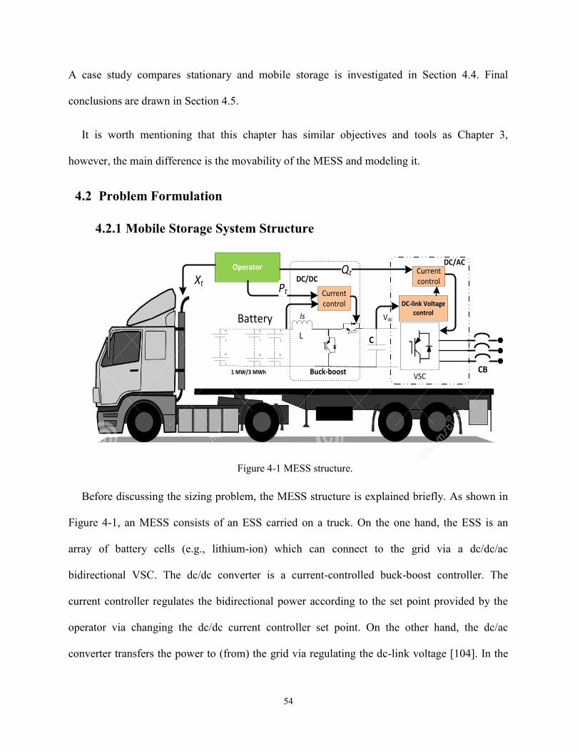
54
A case study compares stationary and mobile storage is investigated in Section 4.4. Final
conclusions are drawn in Section 4.5.
It is worth mentioning that this chapter has similar objectives and tools as Chapter 3,
however, the main difference is the movability of the MESS and modeling it.
4.2 Problem Formulation
4.2.1 Mobile Storage System Structure
VSC
DC/DC
C
DC-link Voltagecontrol
Currentcontrol
Operator
Battery
CB1 MW/3 MWh
Currentcontrol
Is Vdc
Qt
PtXt
L
DC/AC
Buck-boost
Figure 4-1 MESS structure.
Before discussing the sizing problem, the MESS structure is explained briefly. As shown in
Figure 4-1, an MESS consists of an ESS carried on a truck. On the one hand, the ESS is an
array of battery cells (e.g., lithium-ion) which can connect to the grid via a dc/dc/ac
bidirectional VSC. The dc/dc converter is a current-controlled buck-boost controller. The
current controller regulates the bidirectional power according to the set point provided by the
operator via changing the dc/dc current controller set point. On the other hand, the dc/ac
converter transfers the power to (from) the grid via regulating the dc-link voltage [104]. In the

55
dq-frame, the dc-link voltage controller generates the VSC-direct current set point whereas the
operator tunes the reactive power via changing the quadrature current set point, which can also
be controlled autonomously to regulate the terminal voltage, without the operator interference.
Further details on the design of the current and dc-link voltage controllers can be found in
[104]. On the other hand, the operator must define the truck desired bus (station 𝑥𝑡) at each
sample so that the driver moves the MESS to this station. It is worth mentioning that the direct
connection of an MESS to a medium voltage network involves special commissioning
procedures; thus, it is preferred to be connected to a low-voltage network or equipping each
MESS station with a low-voltage terminal via a distribution transformer. An MESS is an
investment conducted by a Disco. The Disco aims at profit maximization while maintaining an
acceptable power quality level (e.g., voltage level). To fulfill this objective, the optimization
problem must consider the participation of the MESS in the following grid-support services:1)
Energy arbitrage. 2) Power loss minimization. 3) Voltage regulation.
4.2.2 MESS Planning Cost Function
The cost function presents the Disco profit during the planning horizon as given in (4.1).
The cost function 𝑝𝑟𝑜 is calculated for each time sample 𝑡 indexed in an operation year 𝑦 in a
certain operation scenario 𝑠𝑐. Each operation scenario 𝑠𝑐 has a certain probability 𝜌𝑠𝑐 such
that ∑ 𝜌𝑠𝑐𝑠𝑐 = 1 . A scenario represents a different load, PV, wind and load power and market
prices combinations.
𝑀𝑎𝑥(𝑝𝑟𝑜 = 𝑖𝑛𝑐 − 𝑐𝑔𝑟𝑖𝑑 − 𝑐𝑀𝐸𝑆)
𝑖𝑛𝑐 =∑𝜌𝑠𝑐∑∑𝑠𝑝𝑠𝑐,𝑦,𝑡∑𝑝𝑠𝑐,𝑦,𝑡𝐿𝑜𝑎𝑑(𝑖)𝜏
𝑖𝑡𝑦𝑠𝑐
𝑐𝑔𝑟𝑖𝑑 =∑𝜌𝑠𝑐∑∑𝑏𝑝𝑠𝑐,𝑦,𝑡𝑝𝑠𝑐,𝑦,𝑡𝑔𝑟𝑖𝑑
𝑡𝑦𝑠𝑐
𝜏
(4.1)
(4.2)

56
𝑐𝑀𝐸𝑆 = 𝐶𝑡𝑟𝑢𝑐𝑘 +∑𝑧𝑀𝐸𝑆(𝑖)𝐹𝐶𝑀𝐸𝑆(𝑖) + 𝐶𝑀𝐸𝑆
𝑀𝑉𝐴⁄ (𝕊𝐸𝑆)𝕊𝐸𝑆
𝑖
+ 𝐶𝑀𝐸𝑆
𝑀𝑊ℎ⁄ (1 + 𝛼𝑇𝑁)𝔼𝑀𝐸𝑆 +∑𝑂&𝑀𝑦
𝑀𝐸𝑆
(1 + 𝐼𝑅)𝑌−1𝑦
(4.3)
(4.4)
The Disco profit results from the income 𝑖𝑛𝑐 coming from selling energy to the end-users as
in (4.2). This income results from selling the load power 𝑝𝑠𝑐,𝑦,𝑡𝐿𝑜𝑎𝑑 with a sell price 𝑠𝑝𝑠𝑐,𝑦,𝑡 that
depends on the Disco tariff. Each Disco buys the power 𝑝𝑠𝑐,𝑦,𝑡𝑔𝑟𝑖𝑑
from the energy market for a
variable wholesale buy price 𝑏𝑝𝑠𝑐,𝑦,𝑡 that witnesses a big change from off-peak to peak hours,
depending on the market volatility. An MESS can perform a load shifting to reduce the cost of
the purchased energy 𝑐𝑔𝑟𝑖𝑑 to increase the profit as in (4.3). Maximizing the profit means
reducing the power loss cost as will be explained later. Finally, 𝑐𝑀𝐸𝑆 is the MESS capital and
running cost that consists of five parts as in
(4.4):
1. The truck capital cost (𝑇𝐶).
2. The MESS stations cost 𝐹𝐶𝑀𝐸𝑆 that includes a fixed cost for each station
constructed and preparation at a certain bus i.
3. The energy storage (ES) power cost 𝐶𝑀𝐸𝑆
𝑀𝑉𝐴⁄ that represents the capital cost for
purchasing the power conversion system of the battery. This cost varies with the
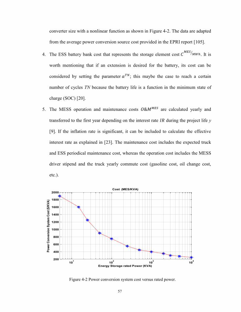
57
converter size with a nonlinear function as shown in Figure 4-2. The data are adapted
from the average power conversion source cost provided in the EPRI report [105].
4. The ESS battery bank cost that represents the storage element cost 𝐶𝑀𝐸𝑆
𝑀𝑊ℎ⁄ . It is
worth mentioning that if an extension is desired for the battery, its cost can be
considered by setting the parameter 𝛼𝑇𝑁; this maybe the case to reach a certain
number of cycles TN because the battery life is a function in the minimum state of
charge (SOC) [20].
5. The MESS operation and maintenance costs 𝑂&𝑀𝑀𝐸𝑆 are calculated yearly and
transferred to the first year depending on the interest rate 𝐼𝑅 during the project life y
[9]. If the inflation rate is significant, it can be included to calculate the effective
interest rate as explained in [23]. The maintenance cost includes the expected truck
and ESS periodical maintenance cost, whereas the operation cost includes the MESS
driver stipend and the truck yearly commute cost (gasoline cost, oil change cost,
etc.).
Figure 4-2 Power conversion system cost versus rated power.
101
102
103
104
200
400
600
800
1000
1200
1400
1600
1800
2000
Energy Storage rated Power (KVA)
Po
we
r C
on
ve
rsio
n S
ys
tem
Co
st
($/K
VA
)
Cost (MES/KVA)

58
4.2.3 MESS Model
The MESS modeling is different from the stationary ESS in that it should be allocated at a
single station as given in (4.5). The constraint in (4.5) states that at any instant t in a planning
year y of a particular scenario sc, the location of the MESS 𝑥𝑠𝑐,𝑦,𝑡𝑀𝐸𝑆 (𝑖) is unique at a single station
of the MESS stations that belongs to the buses set 𝒩𝑀𝐸𝑆. Another important factor is the
number of daily trips DT conducted by the MESS which is expressed in (4.6). If an MESS
stayed the whole day at the same station i=a, then ∑ 𝑥𝑠𝑐,𝑦,𝑡𝑀𝐸𝑆 − 𝑥𝑠𝑐,𝑦,𝑡−1
𝑀𝐸𝑆24𝑡=1 = 0 ∀𝑖 which means
that no trips are made. On the other hand, if the MESS moved from a station a to another one b
at a time 𝛼, then |𝑥𝑠𝑐,𝑦,𝛼+1𝑀𝐸𝑆 (𝑎) − 𝑥𝑠𝑐,𝑦,𝛼
𝑀𝐸𝑆 (𝑎)| = |𝑥𝑠𝑐,𝑦,𝛼+1𝑀𝐸𝑆 (𝑏) − 𝑥𝑠𝑐,𝑦,𝛼
𝑀𝐸𝑆 (𝑏)| = 1 which means that
DT is accumulated by one each time a transition is made. The daily number of trips is upper
bounded in (4.7). It is worth mentioning that there is a transit or delay each time the trip is
made, however; adding an exact delay model significantly complicates the problem; thus, an
instantaneous transition is assumed and the delay effect is investigated later.
∑𝑥𝑠𝑐,𝑦,𝑡𝑀𝐸𝑆 (𝑖)
𝑖
= 1 ∀𝑖 ∈ 𝒩𝑀𝐸𝑆
𝐷𝑇𝑠𝑐,𝑦,𝑡=24 =∑ ∑ |𝑥𝑠𝑐,𝑦,𝑡
𝑀𝐸𝑆 (𝑖) − 𝑥𝑠𝑐,𝑦,𝑡−1𝑀𝐸𝑆 (𝑖)|𝑖
24𝑡=1
2
𝐷𝑇𝑠𝑐,𝑦,𝑡=24 ≤ 𝐷𝑇
(4.5)
(4.6)
(4.7)
The stations location and sizing of an MESS is expressed in (4.8)-(4.10). The binary variable
𝑧𝑀𝐸𝑆(𝑖) indicates that the bus i is chosen to host an MESS station. The number of stations is
limited in (4.8), whereas the station maximum power 𝕊𝑀𝐸𝑆 is upper bounding the MESS rated
power 𝕊𝑀𝐸𝑆 in (4.9). The MESS maximum allowable capacity 𝔼𝑀𝐸𝑆 is expressed in (4.10) .

59
∑𝑧𝑀𝐸𝑆(𝑖) ≤ 𝑧𝑀𝐸𝑆 ∀𝑖 ∈ 𝒩𝑀𝐸𝑆
𝑖
0 ≤ 𝕊𝑀𝐸𝑆 ≤ 𝑧𝑀𝐸𝑆(𝑖)𝕊𝑀𝐸𝑆
0 ≤ 𝔼𝑀𝐸𝑆 ≤ 𝑧𝑀𝐸𝑆(𝑖)𝔼𝑀𝐸𝑆
(4.8)
(4.9)
(4.10)
The MESS power consists of two mutually exclusive terms; the charging power 𝑐ℎ𝑠𝑐,𝑦,𝑡𝑀𝐸𝑆
(positive) and discharging power 𝑑𝑐𝑠𝑐,𝑦,𝑡𝑀𝐸𝑆 (negative) as shown in (4.11). The MESS is only
allowed to charge or discharge at a certain station i if it exists at this station and within the rated
power limit as in (4.12)-(4.13). The reactive power injected/absorbed at any bus for voltage
regulation purposes is similarly constrained in (4.14). Finally, the converter thermal limit is
defined in (4.15). It is worth mentioning that the constraints (4.12)-(4.15) are nonlinear because
both 𝕊𝑀𝐸𝑆and 𝑥𝑠𝑐,𝑦,𝑡𝑀𝐸𝑆 (𝑖) are decision variables.
𝑝𝑠𝑐,𝑦,𝑡𝑀𝐸𝑆 (𝑖) = 𝑐ℎ𝑠𝑐,𝑦,𝑡
𝑀𝐸𝑆 (𝑖) + 𝑑𝑐𝑠𝑐,𝑦,𝑡𝑀𝐸𝑆 (𝑖)
0 ≤ 𝑐ℎ𝑠𝑐,𝑦,𝑡𝑀𝐸𝑆 (𝑖) ≤ 𝕊𝑀𝐸𝑆𝑥𝑠𝑐,𝑦,𝑡
𝑀𝐸𝑆 (𝑖)
−𝕊𝑀𝐸𝑆𝑥𝑠𝑐,𝑦,𝑡𝑀𝐸𝑆 (𝑖) ≤ 𝑑𝑐𝑠𝑐,𝑦,𝑡
𝑀𝐸𝑆 (𝑖) ≤ 0
−𝕊𝑀𝐸𝑆𝑥𝑠𝑐,𝑦,𝑡𝑀𝐸𝑆 (𝑖) ≤ 𝑞𝑠𝑐,𝑦,𝑡
𝑀𝐸𝑆 (𝑖) ≤ 𝕊𝑀𝐸𝑆𝑥𝑠𝑐,𝑦,𝑡𝑀𝐸𝑆 (𝑖)
𝑝𝑠𝑐,𝑦,𝑡𝑀𝐸𝑆 (𝑖)2 + 𝑞𝑠𝑐,𝑦,𝑡
𝑀𝐸𝑆 (𝑖)2 ≤ 𝑥𝑠𝑐,𝑦,𝑡𝑀𝐸𝑆 (𝑖)𝕊𝑀𝐸𝑆2
(4.11)
(4.12)
(4.13)
(4.14)
(4.15)
Regarding the capacity sizing, the MESS capacity at any time sample is defined as an
integrator of the power injected/absorbed at any station i. Both the charging and discharging
efficiencies 𝜂𝑐ℎ, 𝜂𝑑𝑐 are considered as well in (4.16). The MESS capacity is upper-bounded by
its rated value in (4.17). The number of cycles 𝑁𝑀𝐸𝑆 is another integrator that counts the MESS
energy at/from any bus i as in (4.18). When a rated capacity 𝔼𝑀𝐸𝑆 is totally absorbed and

60
injected by the ESS, 𝑁𝑀𝐸𝑆 is incremented by 1× 𝔼𝑀𝐸𝑆. The total ESS number of cycles 𝑇𝑁𝐸𝑆 is
imposed by (4.19).
𝐸𝑠𝑐,𝑦,𝑡+1𝑀𝐸𝑆 = 𝐸𝑠𝑐,𝑦,𝑡
𝑀𝐸𝑆 +∑(𝜂𝑐ℎ𝑐ℎ𝑠𝑐,𝑦,𝑡𝑀𝐸𝑆 (𝑖) + 𝜂𝑑𝑐𝑑𝑐𝑠𝑐,𝑦,𝑡
𝑀𝐸𝑆 (𝑖))𝜏
𝑖
0 ≤ 𝐸𝑠𝑐,𝑦,𝑡𝑀𝐸𝑆 ≤ 𝔼𝑀𝐸𝑆
𝑁𝑠𝑐,𝑦,𝑡𝑀𝐸𝑆 = 𝑁𝑠𝑐,𝑦,𝑡−1
𝑀𝐸𝑆 +∑ (𝜂𝑐ℎ𝑐ℎ𝑠𝑐,𝑦,𝑡
𝑀𝐸𝑆 (𝑖) − 𝜂𝑑𝑐𝑑𝑐𝑠𝑐,𝑦,𝑡𝑀𝐸𝑆 (𝑖))𝜏𝑖
2
∑𝜌𝑠𝑐∑∑𝑁𝑠𝑐,𝑦,𝑡=24𝐸𝑆
𝑡𝑦𝑠𝑐
≤ 𝑇𝑁 𝔼𝑀𝐸𝑆
(4.16)
(4.17)
(4.18)
(4.19)
4.2.4 Final Optimization Problem
Regarding the power flow, the same constraints in (3.34)-(3.48) are adopted here. Further, in
the case of using DGs, SVCs or power imbalance solution, the operation constraints can be
easily added from Section 3.2.
To focus on the MESS sizing problem. It is considered as the only technology under study.
The final optimization problem is shown in (4.20).
max𝕊𝑀𝐸𝑆,𝔼𝑀𝐸𝑆,𝕫𝑀𝐸𝑆,𝕩𝑀𝐸𝑆,ℙ,ℚ,𝕧
(𝑝𝑟𝑜)
𝑠. 𝑡. {𝑀𝐸𝑆𝑆 𝑑𝑦𝑛𝑎𝑚𝑖𝑐𝑎𝑙 𝑚𝑜𝑑𝑒𝑙: (4.5) − (4.19) 𝑃𝑜𝑤𝑒𝑟 𝑓𝑙𝑜𝑤 𝑚𝑜𝑑𝑒𝑙: (3.34) − (3.48)
(4.20)
The decision variables of this problem include the MESS rated power and
capacity 𝕊𝑀𝐸𝑆 , 𝔼𝑀𝐸𝑆, and the MESS stations set 𝕫𝑀𝐸𝑆. Other variables that result from the
optimization process represent the system operation nature during the different scenarios, years
and samples. These variables help the operator to study the system performance under the
planning decision results. These variables include the instantaneous MESS location set 𝕩𝑀𝐸𝑆 =
⋃ 𝑥𝑠𝑐,𝑦,𝑡𝑀𝐸𝑆 (𝑖)𝑆𝑐,𝑦,𝑡,𝑖 and similarly, the active, reactive power, and voltage sets: ℙ𝑀𝐸𝑆 =

61
⋃ 𝑝𝑠𝑐,𝑦,𝑡𝑀𝐸𝑆 (𝑖)𝑆𝑐,𝑦,𝑡,𝑖 , ℚ𝑀𝐸𝑆 = ⋃ 𝑞𝑠𝑐,𝑦,𝑡
𝑀𝐸𝑆 (𝑖)𝕧𝑀𝐸𝑆 = ⋃ 𝑣𝑠𝑐,𝑦,𝑡𝑀𝐸𝑆 (𝑖)𝑆𝑐,𝑦,𝑡,𝑖𝑆𝑐,𝑦,𝑡,𝑖 , and the battery
dynamics, such as the capacity and number of cycles. The final sizing problem (4.20) is a mixed
integer nonlinear problem due to the MESS constraints (4.12)-(4.15). Further, the cost function
is a nonlinear function of the storage rated-power-dependent cost as shown in Figure 4-2. Next,
Section 4.3 presents the proposed algorithm to solve this problem.
4.3 Proposed Algorithm
To convert the problem (4.20) from a mixed-integer nonconvex problem (due to constraints
(4.12)-(4.15) and the nonlinear converter cost) into a convex one, the following technique is
proposed. First, the particle swarm optimization is utilized to detect the optimal MESS rated
power (𝕊𝐸𝑆) and stations optimal locations (𝕫𝑀𝐸𝑆). Using all these variables into (4.20), the
problem will be converted into a mixed-integer convex programming problem which can be
solved easily to find the optimal capacity. This technique mixes the artificial intelligence
method with the gradient-based optimization. The PSO is a smart iterative search method that
changes the decision variables (swarm positions) to optimize (minimize or maximize) a certain
criterion [106]. In this chapter, the PSO changes the MESS rated power and locations such that
the profit is maximized. The proposed algorithm is described in the following steps.
The PSO generates a random initial population of particles 𝕐(𝑗 = 0) which is defined by M
particles size as in (4.21). Each particle at certain iteration j, 𝑦(𝑗) consists of the MESS rated
power 𝕊𝑚𝑀𝐸𝑆(𝑗) with its associated cost and a proposed locations set 𝕫𝑚
𝑀𝐸𝑆(𝑗)as in (4.22).
𝕐(𝑗) = [𝑦1(𝑗), 𝑦2(𝑗),… , 𝑦𝑚(𝑗), … 𝑦𝑀(𝑗)]
𝑦𝑚(𝑗) = [𝕊𝑚𝑀𝐸𝑆(𝑗), 𝕫𝑚
𝑀𝐸𝑆(𝑗)] → 𝑐𝑚 𝑀𝐸𝑆
𝑀𝑉𝐴⁄ (𝑗)
(4.21)
(4.22)

62
To maintain the particles limits, the following constraints in (4.23)-(4.24) are imposed on all
particles to keep the rated power within the allowable range and define the locations binary sets.
0 ≤ 𝕊𝑚𝑀𝐸𝑆(𝑗) ≤ 𝕊𝑀𝐸𝑆
𝕫𝑚𝑀𝐸𝑆(𝑗)𝜖{0,1}
(4.23)
(4.24)
For each particle, the associated profit is calculated by solving the mixed-integer convex
problem in (4.25). The problem is the same as the one in (4.20) after the following
modifications. A) The MESS location set becomes a parameter decided by each particle. B) The
nonlinear constraints (4.12)-(4.15) become convex (linear or quadratic) after considering the
MESS rated power a constant parameter. C) The rated power cost is calculated from an
interpolation table follows Figure 4-2. Now, this problem can be efficiently solved by solvers as
GUROBI [102]. The resulting capacity is also saved for each solution after solving (4.25) as
expressed in (4.26)
max𝔼𝑀𝐸𝑆,𝕩𝑀𝐸𝑆,ℙ,ℚ,𝕧
(𝑝𝑟𝑜𝑚(𝑗) = 𝑝𝑟𝑜(𝑦𝑚(𝑗), 𝑐𝑚 𝑀𝐸𝑆
𝑀𝑉𝐴⁄ (𝑗)))
𝑠. 𝑡.
{
𝑀𝐸𝑆𝑆 𝑑𝑦𝑛𝑎𝑚𝑖𝑐𝑎𝑙 𝑚𝑜𝑑𝑒𝑙: (5) − (7), (10), (11), (16) − (19)
𝑃𝑜𝑤𝑒𝑟 𝑓𝑙𝑜𝑤 𝑚𝑜𝑑𝑒𝑙: (3.34) − (3.48)
ℤ𝑀𝐸𝑆 = 𝕫𝑚𝑀𝐸𝑆(𝑗)
0 ≤ 𝑐ℎ𝑠𝑐,𝑦,𝑡𝑀𝐸𝑆 (𝑖) ≤ 𝕊𝑚
𝑀𝐸𝑆(𝑗)𝑥𝑠𝑐,𝑦,𝑡𝑀𝐸𝑆 (𝑖)
−𝕊𝑚𝑀𝐸𝑆(𝑗)𝑥𝑠𝑐,𝑦,𝑡
𝑀𝐸𝑆 (𝑖) ≤ 𝑑𝑐𝑠𝑐,𝑦,𝑡𝑀𝐸𝑆 (𝑖) ≤ 0
−𝕊𝑚𝑀𝐸𝑆(𝑗)𝑥𝑠𝑐,𝑦,𝑡
𝑀𝐸𝑆 (𝑖) ≤ 𝑞𝑠𝑐,𝑦,𝑡𝑀𝐸𝑆 (𝑖) ≤ 𝕊𝑚
𝑀𝐸𝑆(𝑗)𝑥𝑠𝑐,𝑦,𝑡𝑀𝐸𝑆 (𝑖)
𝑝𝑠𝑐,𝑦,𝑡𝑀𝐸𝑆 (𝑖)2 + 𝑞𝑠𝑐,𝑦,𝑡
𝑀𝐸𝑆 (𝑖)2 ≤ 𝑥𝑠𝑐,𝑦,𝑡𝑀𝐸𝑆 (𝑖)𝕊𝑚
𝑀𝐸𝑆(𝑗)2
𝔼𝑚𝑀𝐸𝑆(𝑗) = {𝔼𝑀𝐸𝑆|arg {max𝔼,𝕩
(𝑝𝑟𝑜𝑚(𝑗))}}
(4.25)
(4.26)
At each iteration J; the local and global best positions are updated as follows:
𝑦𝑙𝑜𝑐(𝑗 = 𝐽) = {𝑦𝛽(𝐽)|𝑝𝑟𝑜𝛽(𝐽) > 𝑝𝑟𝑜𝑚(𝐽)∀𝑚}
𝑦𝐺𝑙𝑜(𝐽) = {𝑦𝛼|𝑝𝑟𝑜𝛼 > 𝑝𝑟𝑜𝑚(𝑗)∀𝑚, ∀𝑗 ≤ 𝐽}
(4.27)
(4.28)

63
Depending on the iteration J, the new inertia 𝜔 and speed vectors 𝑉 are found from (4.29)-
(4.30), the speed is inclined to both the local and global best positions depending on the
factors 𝑐1, 𝑐2. Finally, the speed is used to update all particles positions as shown in (4.32) after
checking its limits in (4.31)
𝜔(𝑗) = 𝜔𝑚𝑎𝑥 −𝜔𝑚𝑎𝑥 −𝜔𝑚𝑖𝑛
𝐽𝑗
𝑉𝑚(𝑗 + 1) = 𝜔(𝑗)𝑉𝑚(𝑗) + 𝑐1𝑟1(𝑦𝑙𝑜𝑐(𝑗) − 𝑦𝑚(𝑗)) + 𝑐2𝑟2(𝑦
𝐺𝑙𝑜(𝑗) − 𝑦𝑚(𝑗))
−𝑉𝑚 ≤ 𝑉𝑚(𝑗 + 1) ≤ 𝑉𝑚𝑦𝑚(𝑗 + 1) = 𝑉𝑚(𝑗 + 1) + 𝑦𝑚(𝑗)
(4.29)
(4.30)
(4.31)
(4.32)
Step 2 is repeated as long as the stopping criterion is not triggered. There are two stopping
criteria. First, if the maximum number of iterations 𝑗 reached. Second, if the profit percentage
change stayed within a pre-calculated tolerance zone 𝜀 for a certain number of iterations 𝛾 as
explained in (4.34).
𝑗 ≥ 𝑗
∆𝑝𝑟𝑜𝐺𝑙𝑜(𝑗: 𝑗 + 𝛾) ≤ 𝜀, 𝑗 + 𝛾 ≤ 𝑗
(4.33)
(4.34)
Finally, if the stopping criterion is achieved, an optimum sizing and allocation decision is
reached. Figure 4-3 shows the flowchart of the proposed optimization framework.
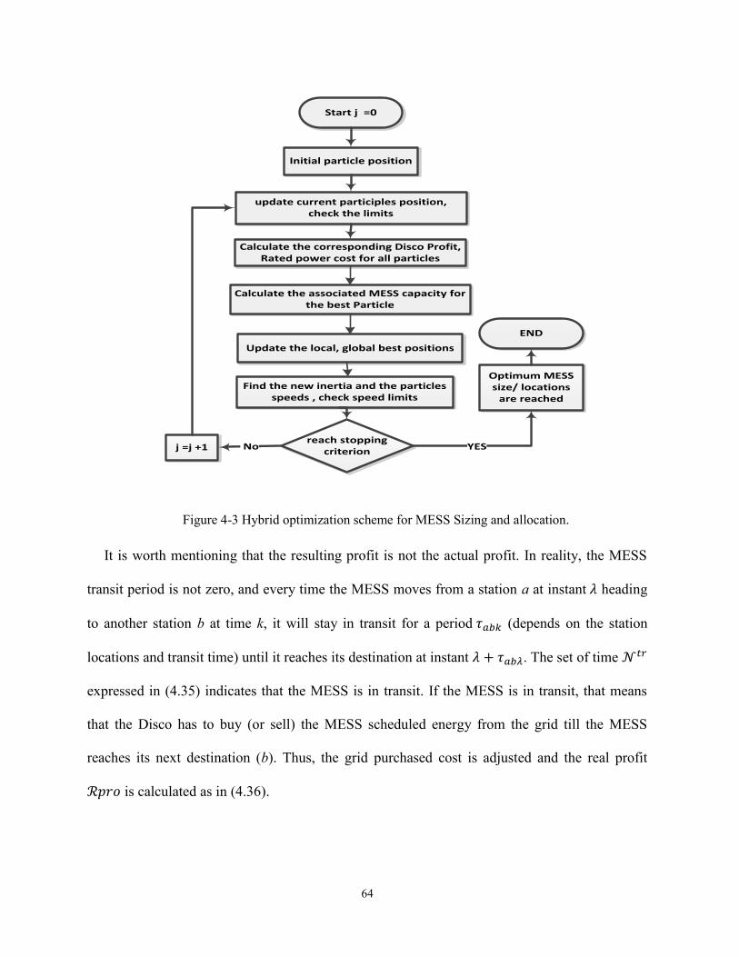
64
Start j =0
Initial particle position
update current participles position, check the limits
Calculate the corresponding Disco Profit, Rated power cost for all particles
Update the local, global best positions
Find the new inertia and the particles speeds , check speed limits
j =j +1 reach stopping
criterion
Optimum MESS size/ locations
are reached
END
No YES
Calculate the associated MESS capacity for the best Particle
Figure 4-3 Hybrid optimization scheme for MESS Sizing and allocation.
It is worth mentioning that the resulting profit is not the actual profit. In reality, the MESS
transit period is not zero, and every time the MESS moves from a station a at instant 𝜆 heading
to another station b at time k, it will stay in transit for a period 𝜏𝑎𝑏𝑘 (depends on the station
locations and transit time) until it reaches its destination at instant 𝜆 + 𝜏𝑎𝑏𝜆. The set of time 𝒩𝑡𝑟
expressed in (4.35) indicates that the MESS is in transit. If the MESS is in transit, that means
that the Disco has to buy (or sell) the MESS scheduled energy from the grid till the MESS
reaches its next destination (b). Thus, the grid purchased cost is adjusted and the real profit
ℛ𝑝𝑟𝑜 is calculated as in (4.36).
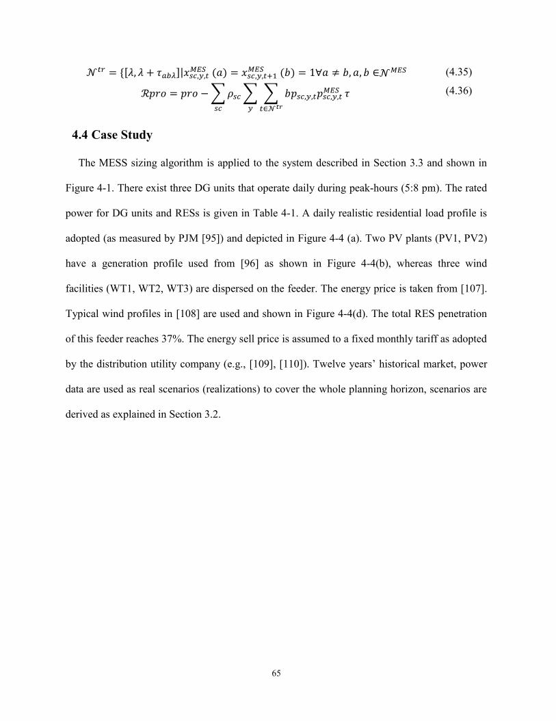
65
𝒩𝑡𝑟 = {[𝜆, 𝜆 + 𝜏𝑎𝑏𝜆]|𝑥𝑠𝑐,𝑦,𝑡𝑀𝐸𝑆 (𝑎) = 𝑥𝑠𝑐,𝑦,𝑡+1
𝑀𝐸𝑆 (𝑏) = 1∀𝑎 ≠ 𝑏, 𝑎, 𝑏 ∈𝒩𝑀𝐸𝑆
ℛ𝑝𝑟𝑜 = 𝑝𝑟𝑜 −∑𝜌𝑠𝑐∑ ∑ 𝑏𝑝𝑠𝑐,𝑦,𝑡𝑝𝑠𝑐,𝑦,𝑡𝑀𝐸𝑆
𝑡∈𝒩𝑡𝑟𝑦𝑠𝑐
𝜏
(4.35)
(4.36)
4.4 Case Study
The MESS sizing algorithm is applied to the system described in Section 3.3 and shown in
Figure 4-1. There exist three DG units that operate daily during peak-hours (5:8 pm). The rated
power for DG units and RESs is given in Table 4-1. A daily realistic residential load profile is
adopted (as measured by PJM [95]) and depicted in Figure 4-4 (a). Two PV plants (PV1, PV2)
have a generation profile used from [96] as shown in Figure 4-4(b), whereas three wind
facilities (WT1, WT2, WT3) are dispersed on the feeder. The energy price is taken from [107].
Typical wind profiles in [108] are used and shown in Figure 4-4(d). The total RES penetration
of this feeder reaches 37%. The energy sell price is assumed to a fixed monthly tariff as adopted
by the distribution utility company (e.g., [109], [110]). Twelve years’ historical market, power
data are used as real scenarios (realizations) to cover the whole planning horizon, scenarios are
derived as explained in Section 3.2.

66
Figure 4-4 Single line diagram for the distribution feeder under study.
Regarding the MESS, the lithium-ion battery is adopted due to its high energy intensity, high
efficiency, and long life. The battery technical and economic data are taken from [100]. The
storage life cycles are 3000 life cycles during the planning period. The power conversion cost
follows Figure 4-2, whereas the yearly operation and maintenance cost is assumed 12 k$/year
(assuming a part-time driver with two hours duty daily), and the truck capital cost is assumed 50
k$. For MESS stations allocation, ten buses are chosen as candidates as given in Table 4-1; only
three buses are allowed as MESS stations. The PSO parameters are set using a trial and error
approach, and the population size was found to provide an adequate computational time for this
particular problem. For defining the MESS daily number of trips 𝐷��, the minimum value is
desirable given that it achieves the maximum profit and guarantees a feasible solution. Here, 𝐷𝑇
was found to be four. The sizing problem of the MESS using the proposed algorithm is solved
by the Gurobi solver in 6 hours and 35 minutes using a 3.30 GHz AMD six-core processor. The
solver gap from the global optimal is recorded as 0.39%.

67
Table 4-1 Optimization input parameters.
RES,
DG units
rating
𝑝𝑤𝑡1 = 2𝑀𝑊, 𝑝𝑤𝑡2 = 𝑝𝑤𝑡3 = 1.5𝑀𝑊, 𝑝𝐷𝐺1 = 1 𝑀𝑊
𝑝𝑝𝑣1 = 𝑝𝑝𝑣2 = 0.5 𝑀𝑊, 𝑝𝐷𝐺2 = 𝑝𝐷𝐺3 = 0.5 𝑀𝑊
𝒩𝑀𝐸𝑆 𝑐𝑎𝑛𝑑𝑖𝑑𝑎𝑡𝑒𝑠 = {4, 6, 9, 12, 22, 25, 28, 35, 39, 40}
MESS
Data
𝑣 = 0.95, �� = 1.05, 𝜏 = 1, 𝐼𝑅 = 3%, 𝑌 = 12, 𝑆𝑐 = 48,
𝕊𝑀𝐸𝑆 = 5 𝑀𝑉𝐴, 𝔼𝐸𝑆 = 15𝑀𝑊ℎ, 𝐹𝐶𝑀𝐸𝑆 = 5000$,
𝐶𝑡𝑟𝑢𝑐𝑘 = 50𝐾$, 𝐷𝑇 = 4, 𝛼𝑇𝑁 = 20%
𝐷𝑁𝑀𝐸𝑆 = 1, 𝑇𝑁𝑀𝐸𝑆 = 3000, 𝑧𝑀𝐸𝑆 = 3, 𝑂&𝑀𝑀𝐸𝑆 = 12𝑘$ 𝑦⁄
𝐶𝑀𝐸𝑆
𝑀𝑊ℎ⁄ = 600 𝐾$, 𝜂 = 0.85
PSO
Data
𝐽 = 200, 𝑐1 = 𝑐2 = 2,𝜔𝑚𝑎𝑥 = 0.9, 𝜔𝑚𝑖𝑛 = 0.1
𝑀 = 10, 𝛾 = 8, 𝜀 = 0.25%, 𝑉𝑚 = [0.5 ∗ 𝑜𝑛𝑒𝑠(10,1); 1 ]
Two cases are compared in Table 4-2 during the whole operation period, which includes the
MESS and stationary ESSs (SESSs). The SESS sizing and allocation is same as the MESS with
changing the size, allocation constraints with theses used in [9]. Because the MESS is a
centralized ESS, it has a higher power rating which yields a less per unit power-converter cost.
It is interesting how the SESS has a higher converter total cost although its aggregated power
rating is less that in the MESS. The saving in the power converter cost alone reached 200 k$
which is the main reason in the profit privilege of the MESS. Because the optimal MESS size is
higher than the equivalent SESS size, the MESS has managed to gain greater arbitrage benefit
and was capable of achieving higher losses reduction because it improves the voltage profile.
Further, a significant maximum load reduction is reached which may defer the substation or
feeder upgrade cost as well. The MESS has achieved 1.38 times the equivalent SESS profit.
Regarding the MESS stations allocations, three locations are selected by the optimization
algorithm; one near the feeder substation {bus 9}, while the other two at the end of each lateral
(buses 28, 40). This result makes senses because the MESS is supposed to provide a reactive

68
power support for voltage regulation at the weakest buses. Regarding the optimality of the
resulting MESS sizing, Figure 4-4 compares the profit with different MESS power ratings. It
can be concluded that the proposed algorithm has managed to define an optimum solution.
Table 4-2. Optimization Results With different ESS Technologies.
MESS Stationary-ESSs
Rated power 3250 kVA 727, 595, 1500 kVA: 2822 kVA (Total)
Capacity 6381.3 kWh 1455, 1190, 3000 kWh: 5645 kWh (Total)
Optimal locations 9 (St.1), 28 (St.2), 40 (St.3) 28, 39, 40
Power converter cost 418,220$ 618,300$
Battery bank cost 3,828,780$ 3,387,000$
Total Storage cost 4,247,000 $ 4,005,300 $
Losses reduction 47.22% 45.17 %
Max. Load reduction 4.38% 4.39 %
Saved losses 2,092,500 $ 1,985,600 $
Arbitrage profit 2,919,800 $ 2,570,800 $
Total profit 10,138,000$ 9,923,500 $
Profit increase 765,400 $ 550,900 $
To monitor the dynamic performance of the MESS that results from the sizing discussion, a
winter day scenario is shown in Figure 4-6. During this scenario, the MESS shifts late night
energy to the afternoon peak hour to achieve arbitrage profit as shown in Figure 4-6 (b).
Regarding the MESS location transitions, first, the MESS provides a leading reactive power
support at the far end of the feeder (Station 3 or bus 40) then it moves to bus 9 to start charging.
The reason for this transition is reducing the power loss by choosing a charging location near
the main substation. The second transition is made to bus 28 (Station 2) near WT3 where the

69
Extra wind power is saved for peak hours. After charging the surplus wind energy, the MESS
moves to the feeder end (at Station 3 located at bus 40) where the MESS performs voltage
regulation with energy arbitrage (discharging stored off-peak energy during the peak hour).
The number of the MESS trips is kept four as given in the optimization constraints and
depicted in Figure 4-6(d). Besides, the capacity is upper-bounded by the rated value, and the
number of charging cycles is one as shown in Figure 4-6(e).
2.5 3 3.5 4 4.5 5
9.94
9.96
9.98
10
10.02
10.04
10.06
10.08
10.1
10.12
10.14
MESS Rating (MVA)
Pro
fit
(Millio
n $
)
Profit Change with MESS power rating
Figure 4-5 MESS rated power verses Profit.
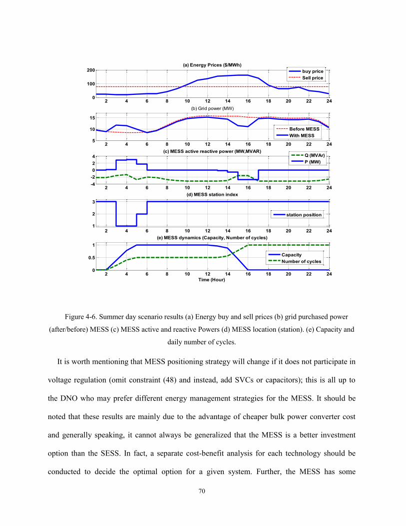
70
Figure 4-6. Summer day scenario results (a) Energy buy and sell prices (b) grid purchased power
(after/before) MESS (c) MESS active and reactive Powers (d) MESS location (station). (e) Capacity and
daily number of cycles.
It is worth mentioning that MESS positioning strategy will change if it does not participate in
voltage regulation (omit constraint (48) and instead, add SVCs or capacitors); this is all up to
the DNO who may prefer different energy management strategies for the MESS. It should be
noted that these results are mainly due to the advantage of cheaper bulk power converter cost
and generally speaking, it cannot always be generalized that the MESS is a better investment
option than the SESS. In fact, a separate cost-benefit analysis for each technology should be
conducted to decide the optimal option for a given system. Further, the MESS has some
2 4 6 8 10 12 14 16 18 20 22 240
100
200(a) Energy Prices ($/MWh)
2 4 6 8 10 12 14 16 18 20 22 245
10
15
(b) Grid power (MW)
2 4 6 8 10 12 14 16 18 20 22 24-4
-2
0
2
4(c) MESS active reactive power (MW,MVAR)
2 4 6 8 10 12 14 16 18 20 22 241
2
3
(d) MESS station index
2 4 6 8 10 12 14 16 18 20 22 240
0.5
1
Time (Hour)
(e) MESS dynamics (Capacity, Number of cycles)
buy price
Sell price
Before MESS
With MESS
Q (MVAr)
P (MW)
station position
Capacity
Number of cycles

71
reliability disadvantage due to its transition from a station to another (transition delay). Finally,
the MESS cannot always guarantee a successful replacement for a large number of SESSs, as
more than one MESS can be required to have different positions in enormous power systems.
This point will be investigated in future research.
4.5 Conclusion
This chapter proposed a sizing and allocation algorithm for a mobile energy storage system
in the distribution system. The optimization aimed at maximizing the utility profit by
considering the participation of the MESS in multi grid-support services including energy
arbitrage, voltage regulation, and power loss minimization. The sizing constraints included the
battery life cycles and dynamic capacity, and the feeder voltage levels and ampacity. Load and
renewable energy variations were modeled via considering different scenarios in the sizing
scheme. Further, a size-dependent cost for the power converter was adopted which is more
realistic and practical. The sizing algorithm was tested by a case study on a real radial feeder
using realistic power and market price data. The study results showed that using the MESS may
yield a higher profit than stationary ESSs due to its low bulk power conversion cost while
providing multi-tasking as in multi-stationary ESSs. Future research will consider the same
problem with multi mobile storage units with more sophisticated transit delay models.
72
Chapter 5
5 EMS of a Hybrid Wind-Battery Energy Storage System via
Model Predictive Control
5.1 Introduction
This chapter presents a market-oriented energy management system (EMS) for a hybrid
power system composed of a wind energy conversion system (WECS) and a battery energy
storage system (BESS). The EMS is designed as a real-time model predictive control (MPC)
system. The EMS dispatches the BESS to achieve the maximum net profit from the deregulated
electricity market for the owner (RES energy time shifting). For net profit maximization, the
EMS aims at expanding the BESS lifetime by applying typical and practical constraints in the
MPC problem on both the daily number of cycles (DNC) and depth of discharge (DOD). These
constraints are vital because the BESS life is a function in both the DNC and the DOD. The
MPC constraints optimizer is designed to tune these lifetime constraints optimally to achieve
the maximum market revenue with a minimal expended-life cost. The effectiveness of this work
is verified by comparison with a conventional MPC used in previous works. A simulation study
is conducted using a real wind power and market data in Alberta, Canada. The new
contributions of this work to the research field are:
1) A detailed storage cost is calculated and considered in the optimization problem.
Further, the expended-life cost, which is a function in the DNC and DOD, has also examined
for obtaining an accurate and practical economic cost function.
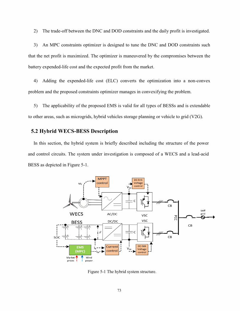
73
2) The trade-off between the DNC and DOD constraints and the daily profit is investigated.
3) An MPC constraints optimizer is designed to tune the DNC and DOD constraints such
that the net profit is maximized. The optimizer is maneuvered by the compromises between the
battery expended-life cost and the expected profit from the market.
4) Adding the expended-life cost (ELC) converts the optimization into a non-convex
problem and the proposed constraints optimizer manages in convexifying the problem.
5) The applicability of the proposed EMS is valid for all types of BESSs and is extendable
to other areas, such as microgrids, hybrid vehicles storage planning or vehicle to grid (V2G).
5.2 Hybrid WECS-BESS Description
In this section, the hybrid system is briefly described including the structure of the power
and control circuits. The system under investigation is composed of a WECS and a lead-acid
BESS as depicted in Figure 5-1.
Figure 5-1 The hybrid system structure.
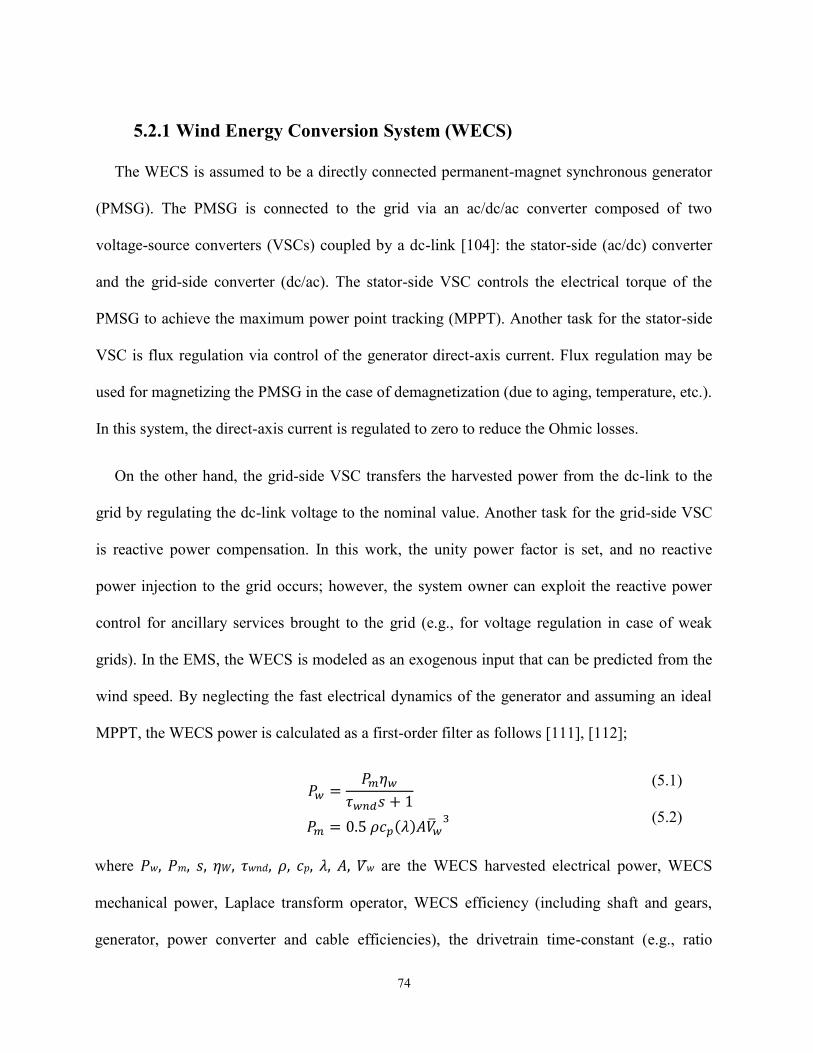
74
5.2.1 Wind Energy Conversion System (WECS)
The WECS is assumed to be a directly connected permanent-magnet synchronous generator
(PMSG). The PMSG is connected to the grid via an ac/dc/ac converter composed of two
voltage-source converters (VSCs) coupled by a dc-link [104]: the stator-side (ac/dc) converter
and the grid-side converter (dc/ac). The stator-side VSC controls the electrical torque of the
PMSG to achieve the maximum power point tracking (MPPT). Another task for the stator-side
VSC is flux regulation via control of the generator direct-axis current. Flux regulation may be
used for magnetizing the PMSG in the case of demagnetization (due to aging, temperature, etc.).
In this system, the direct-axis current is regulated to zero to reduce the Ohmic losses.
On the other hand, the grid-side VSC transfers the harvested power from the dc-link to the
grid by regulating the dc-link voltage to the nominal value. Another task for the grid-side VSC
is reactive power compensation. In this work, the unity power factor is set, and no reactive
power injection to the grid occurs; however, the system owner can exploit the reactive power
control for ancillary services brought to the grid (e.g., for voltage regulation in case of weak
grids). In the EMS, the WECS is modeled as an exogenous input that can be predicted from the
wind speed. By neglecting the fast electrical dynamics of the generator and assuming an ideal
MPPT, the WECS power is calculated as a first-order filter as follows [111], [112];
𝑃𝑤 =𝑃𝑚𝜂𝑤
𝜏𝑤𝑛𝑑𝑠 + 1
𝑃𝑚 = 0.5 𝜌𝑐𝑝(𝜆)𝐴��𝑤3
(5.1)
(5.2)
where 𝑃𝑤, 𝑃𝑚, 𝑠, 𝜂𝑊, 𝜏𝑤𝑛𝑑, 𝜌, 𝑐𝑝, 𝜆, 𝐴, 𝑉�� are the WECS harvested electrical power, WECS
mechanical power, Laplace transform operator, WECS efficiency (including shaft and gears,
generator, power converter and cable efficiencies), the drivetrain time-constant (e.g., ratio

75
between the shaft inertia and friction), air density, power coefficient, tip speed ratio, rotor disk
area and the effective wind speed across the rotor disk. Further details are explained in [111].
The dominant dynamics of the WECS are modeled as a first-order filter with 𝑃𝑚 representing the
input disturbance to the system [112] 𝜏𝑤𝑛𝑑 is assumed to be 1.5 s and 𝜂𝑤 = 0.9.
5.2.2 Battery Energy Storage System (BESS)
The BESS consists of an array of lead-acid cells. The array terminal voltage is determined by
the number of series cells in the same string, whereas the total current is the sum of the parallel
strings currents. The reader is referred to the IEEE Standard 485 [113] for more information on
the BESS sizing. The BESS is connected to the grid via a dc/dc/ac bidirectional VSC. The dc/dc
converter is a current-controlled buck-boost controller. The current controller regulates the
charging (discharging) power according to the set point provided by the EMS. On the other
hand, the ac/dc converter transfers the power to (from) the grid via regulation of the dc-link
voltage [104]. Further, the system owner can exploit the reactive power control for ancillary
services brought to the grid for reactive power support; however, the proposed work does not
investigate the participation in these services, which may require certain BESS rating
requirements [40]. All controllers above (current, MPPT and voltage controllers) are relatively
fast (have very wide bandwidth) with respect to the EMS speed. Thus, the internal dynamics of
all these are constant from the EMS point of view. As a result, the battery storage dynamics are
only considered in the EMS design model.
Any battery has a non-linear time-variant model due to sophisticated parasitic chemical
losses and the unmodeled temperature-dependent dynamics [114], [115]. The authors of [115]
derived a system identification model for the lead-acid battery using experimental
measurements over ten years of experimental results. The resulting model is a third-order state
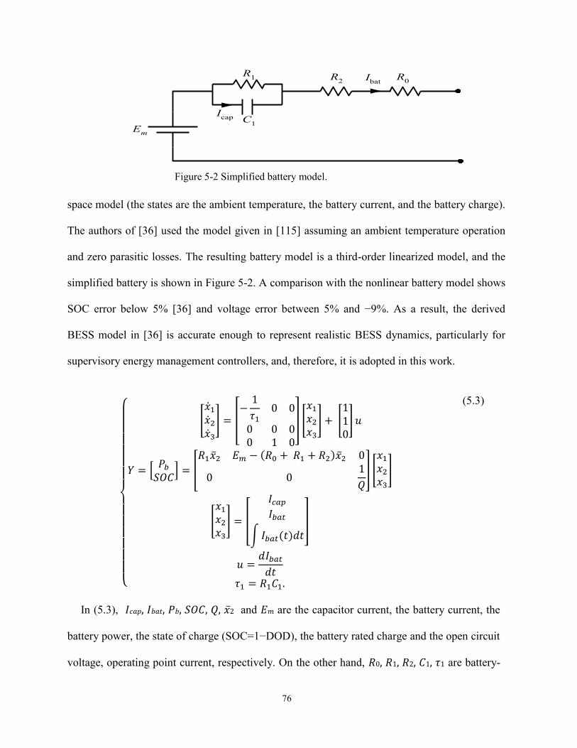
76
space model (the states are the ambient temperature, the battery current, and the battery charge).
The authors of [36] used the model given in [115] assuming an ambient temperature operation
and zero parasitic losses. The resulting battery model is a third-order linearized model, and the
simplified battery is shown in Figure 5-2. A comparison with the nonlinear battery model shows
SOC error below 5% [36] and voltage error between 5% and −9%. As a result, the derived
BESS model in [36] is accurate enough to represent realistic BESS dynamics, particularly for
supervisory energy management controllers, and, therefore, it is adopted in this work.
{
[
��1��2��3
] = [−1
𝜏10 0
0 0 00 1 0
] [
𝑥1𝑥2𝑥3] + [
110] 𝑢
𝑌 = [𝑃𝑏𝑆𝑂𝐶
] = [
𝑅1��2 𝐸𝑚 − (𝑅0 + 𝑅1 + 𝑅2)��2 0
0 01
𝑄
] [
𝑥1𝑥2𝑥3]
[
𝑥1𝑥2𝑥3] = [
𝐼𝑐𝑎𝑝𝐼𝑏𝑎𝑡
∫𝐼𝑏𝑎𝑡(𝑡)𝑑𝑡
]
𝑢 =𝑑𝐼𝑏𝑎𝑡𝑑𝑡
𝜏1 = 𝑅1𝐶1.
(5.3)
In (5.3), 𝐼𝑐𝑎𝑝, 𝐼𝑏𝑎𝑡, 𝑃𝑏, 𝑆𝑂𝐶, 𝑄, ��2 and 𝐸𝑚 are the capacitor current, the battery current, the
battery power, the state of charge (SOC=1−DOD), the battery rated charge and the open circuit
voltage, operating point current, respectively. On the other hand, 𝑅0, 𝑅1, 𝑅2, 𝐶1, 𝜏1 are battery-
R1 R
2R
0
C1
Em
Ibat
Icap
Figure 5-2 Simplified battery model.
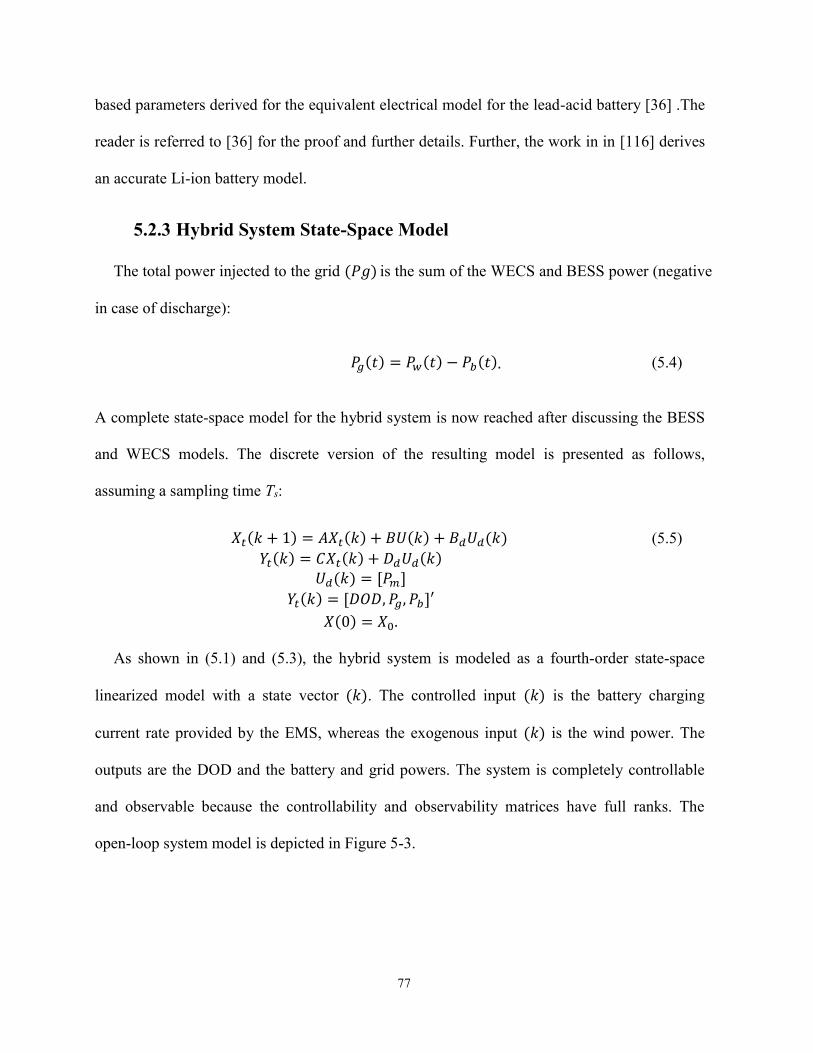
77
based parameters derived for the equivalent electrical model for the lead-acid battery [36] .The
reader is referred to [36] for the proof and further details. Further, the work in in [116] derives
an accurate Li-ion battery model.
5.2.3 Hybrid System State-Space Model
The total power injected to the grid (𝑃𝑔) is the sum of the WECS and BESS power (negative
in case of discharge):
𝑃𝑔(𝑡) = 𝑃𝑤(𝑡) − 𝑃𝑏(𝑡). (5.4)
A complete state-space model for the hybrid system is now reached after discussing the BESS
and WECS models. The discrete version of the resulting model is presented as follows,
assuming a sampling time Ts:
𝑋𝑡(𝑘 + 1) = 𝐴𝑋𝑡(𝑘) + 𝐵𝑈(𝑘) + 𝐵𝑑𝑈𝑑(𝑘)
𝑌𝑡(𝑘) = 𝐶𝑋𝑡(𝑘) + 𝐷𝑑𝑈𝑑(𝑘)
𝑈𝑑(𝑘) = [𝑃𝑚]
𝑌𝑡(𝑘) = [𝐷𝑂𝐷, 𝑃𝑔, 𝑃𝑏]′
𝑋(0) = 𝑋0.
(5.5)
As shown in (5.1) and (5.3), the hybrid system is modeled as a fourth-order state-space
linearized model with a state vector (𝑘). The controlled input (𝑘) is the battery charging
current rate provided by the EMS, whereas the exogenous input (𝑘) is the wind power. The
outputs are the DOD and the battery and grid powers. The system is completely controllable
and observable because the controllability and observability matrices have full ranks. The
open-loop system model is depicted in Figure 5-3.
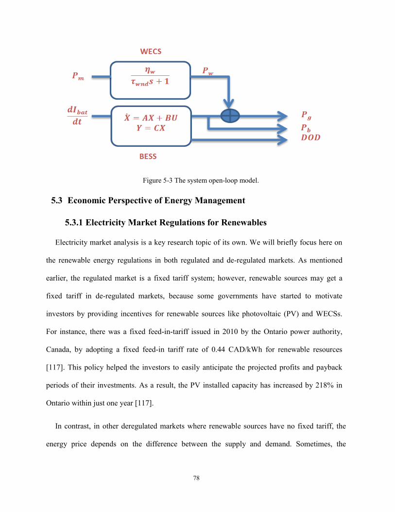
78
Figure 5-3 The system open-loop model.
5.3 Economic Perspective of Energy Management
5.3.1 Electricity Market Regulations for Renewables
Electricity market analysis is a key research topic of its own. We will briefly focus here on
the renewable energy regulations in both regulated and de-regulated markets. As mentioned
earlier, the regulated market is a fixed tariff system; however, renewable sources may get a
fixed tariff in de-regulated markets, because some governments have started to motivate
investors by providing incentives for renewable sources like photovoltaic (PV) and WECSs.
For instance, there was a fixed feed-in-tariff issued in 2010 by the Ontario power authority,
Canada, by adopting a fixed feed-in tariff rate of 0.44 CAD/kWh for renewable resources
[117]. This policy helped the investors to easily anticipate the projected profits and payback
periods of their investments. As a result, the PV installed capacity has increased by 218% in
Ontario within just one year [117].
In contrast, in other deregulated markets where renewable sources have no fixed tariff, the
energy price depends on the difference between the supply and demand. Sometimes, the

79
electricity market can be very volatile and highly unanticipated [39]. Further, the de-regulated
market behavior changes during different seasons and between working days and weekends
[118]. Some countries have a daily de-regulated market where the market closes on a day-ahead
energy commitment. In contrast, other countries run a continuous market with gate closure
where an energy commitment is made periodically each fixed time before the actual delivery.
After gate closure, no other bids are allowed, and the committed energy must be delivered to the
participants [30]. Gate closure has distinct values from one country to another. For instance, a
gate closure occurs each five minutes in Australia and Nord Pool Spot, each hour in the United
Kingdom and some United States regions, each four hours in Spain [30] and each two hours in
Alberta, Canada. The failure of energy commitment after gate closure leads to power-system
imbalance; thus, the system operator must compensate this imbalance using the available
spinning reserve. The compensation cost is collected as a penalty from the participants who
failed to fulfill their energy commitment (mainly PV and WECS facilities). In Alberta, different
regulations exist for WECS integration [119], [120]. A WECS does not bid in the market
because it is non-dispatchable; thus, the wind energy is traded with the current existing price
market (price-taker) [119]. Further, each WECS must declare its system wind power limit
(SWPL) to the Alberta Electric System Operator (AESO). The SWPL is updated to the AESO
each 20 minutes [119] and the exported wind power should not exceed 115% of the stated
SWPL [120]. An EMS controls the SWPL by wind energy curtailment techniques [120].
5.3.2 Energy Storage Cost Calculation
The storage cost study should be comprehensive to include all initial and running costs. This
study was investigated before in [38]; however, it assumed a fixed DOD and DNC operation.
Thus, in this section, we will modify the rules of [38] by adding the BESS expended-life

80
constraints in [121]. Here, the cost is divided into two categories: first, a fixed storage cost
(SC) that includes power converters, balance of operation, replacement cost and maintenance
costs; second, a BESS expended-life cost (ELC) that depends on the depletion in the storage
unit cost due to the EMS. For ensuring a profitable hybrid power system, an optimal sizing for
BESS is required to determine the rated power and capacity of the BESS. The optimal sizing of
a Lead-acid BESS was discussed before in [122]. By adopting the technique in [122], or any
other technique, it is possible to determine the power and capacity of the BESS; these values
determine the annual capital cost of the project (excluding storage cost) as follows [38]:
𝐴𝐶𝐶 = (𝑃𝐶𝑆 + 𝐵𝑂𝑃)𝐶𝑅𝐹 𝐵𝑂𝑃 = 𝐵𝑂𝑃𝑢𝑄 𝑃𝐶𝐶 = 𝑃𝐶𝐶𝑢𝑃𝑟
𝐶𝑅𝐹 =𝑖𝑟(1 + 𝑖𝑟)𝑦
(1 + 𝑖𝑟)𝑦 − 1
(5.6)
(5.7)
(5.8)
(5.9)
where 𝐴𝐶𝐶, 𝑃𝐶𝐶, 𝑃𝐶𝐶𝑢, 𝐵𝑂𝑃, 𝐵𝑂𝑃𝑢, 𝐶𝑅𝐹, 𝑦, 𝑃𝑟, and 𝑖𝑟 are the annual capital cost, power
converter (total $ and per-unit $/kW) cost, balance of plant (total $ and per-unit $/kWh) cost,
capital recovery rate, the project lifetime in years, BESS rated power, and the interest rate,
respectively. The expended-life (EL) of a lead-acid BESS is a function in both the DOD and
DNC and calculated as follows [121]:
𝐸𝐿(𝑁,𝐷𝑂𝐷) =𝑁
𝑁𝑡(𝐷𝑂𝐷)
𝑁𝑡(𝐷𝑂𝐷) = 𝑎 ∗ 𝐷𝑂𝐷 + 𝑏
(5.10)
(5.11)
where 𝑁𝑡 is the battery total number of cycles as a function of the DOD, and a and b are
constants depending on the battery type, characteristics and the total number of cycles at the
nominal DOD (taken 3200 cycle here) [121]. The 𝐷𝑂𝐷 has different forms for other types of
batteries (Lithium-Ion or NiMH batteries) which are stated in [121]. The relation between the
expended-life with the DOD and DNC is depicted in Figure 5-4.
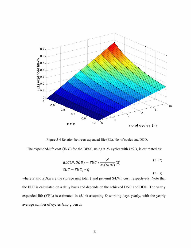
81
Figure 5-4 Relation between expended-life (EL), No. of cycles and DOD.
The expended-life cost (𝐸𝐿𝐶) for the BESS, using it N- cycles with DOD, is estimated as:
𝐸𝐿𝐶(𝑁, 𝐷𝑂𝐷) = 𝑆𝑈𝐶 ∗𝑁
𝑁𝑡(𝐷𝑂𝐷)($)
𝑆𝑈𝐶 = 𝑆𝑈𝐶𝑢 ∗ 𝑄
(5.12)
(5.13)
where 𝑆 and 𝑆𝑈𝐶𝑢 are the storage unit total $ and per-unit $/kWh cost, respectively. Note that
the ELC is calculated on a daily basis and depends on the achieved DNC and DOD. The yearly
expended-life (YEL) is estimated in (5.14) assuming D working days yearly, with the yearly
average number of cycles 𝑁𝑎𝑣𝑔 given as

82
𝑌𝐸𝐿 =𝑁𝑎𝑣𝑔𝐷
𝑁𝑡(𝐷𝑂𝐷𝑎𝑣𝑔) (pu/year). (5.14)
Assuming a fixed yearly number of cycles, given the YEL, the battery replacement times
(BRT) during the project lifetime (y years) is predictable from the desired period of service and
the depletion period for the battery bank. Further, the wearing period of the BESS (WP) is
estimated easily as the time of years to reach 100% depletion as in (5.16).
𝐵𝑅𝑇 = 𝑌𝐸𝐿 ∗ 𝑦 − 1
𝑊𝑃 =1
𝑌𝐸𝐿 (𝑦𝑒𝑎𝑟𝑠)
(5.15)
(5.16)
In the case of a non-integer BRT, it is rounded up and the project lifetime is extended. In
such a case, y is updated and equation (5.9) is re-calculated. After deciding the BRT, the annual
replacement cost (ARC) is calculated, given the future BESS cost (𝐹𝐵𝐶) [38]:
𝐴𝑅𝐶 = 𝐶𝑅𝐹 ∗ 𝐹𝐵𝐶 ∗ 𝑄 ∗∑(1 + 𝑖𝑟)−𝑗∗𝑊𝑃
𝐵𝑅𝑇
𝑗=1
(5.17)
Finally, the storage cost is obtained from the ACC, ARC and the annual operation and
maintenance cost (𝑂&𝑀𝐶), given the annual discharged energy (ADE) [38]:
𝑆𝐶 =𝐴𝐶𝐶 + 𝑂&𝑀𝐶 + 𝐴𝑅𝐶
𝐴𝐷𝐸($/𝐾𝑊ℎ)
𝐴𝐷𝐸 = 𝑄𝑁𝑎𝑣𝑔𝐷
(5.18)
(5.19)
5.4 Proposed Energy Management System Design
This section explains the proposed EMS, which is designed to achieve multiple objectives.
First, the primary objective of the EMS is to maximize the profit of the hybrid system owner
from the deregulated market. The EMS utilizes the available forecast of wind power and
market prices for profit maximization (energy arbitrage). In this work, the prediction horizon is
taken as an hourly forecast for the incoming 24 hours; however, different time frames and

83
sampling intervals are also applicable depending on the data availability and the market
operation. Second, the EMS must dispatch the BESS within acceptable safe power and energy
constraints. Third, the EMS must maximize the BESS lifetime by adopting the minimal DNC
and DOD as long as a feasible solution exists. Finally, the EMS is only allowed to increase the
DOD or DNC if a potential profit higher than the ELC exists. For real-time utilization of the
changing market price and wind power forecast, an MPC is utilized to design the EMS. The
motive of using the MPC will be briefly explained in the upcoming subsection, and then the
problem formulation is discussed. Finally, the proposed constraints optimizer is designed.
5.4.1 A Glance over MPC
A finite horizon MPC is used as an EMS [123]. The MPC is a control technique that is
helpful in case of knowing the controlled output desired trajectory for the incoming prediction
horizon (𝑛𝑝).
Thus, the controller predicts the output of the system for this horizon (iteratively using the state-
space model) at the current instant, assuming ideal modeling, as follows:
𝕪 = [𝑌(𝑘|𝑘), 𝑌(𝑘 + 1|𝑘),… , 𝑌(𝑘 + 𝑛𝑝|𝑘)] (5.20)
It should be noted that 𝕪 is a function in the control action vector (𝕦) and the predicted state
vector (𝕏). The MPC generates the control action for the incoming control horizon 𝑛𝑐 as
follows:
𝕦 = [𝑈(𝑘|𝑘), 𝑈(𝑘 + 1|𝑘), … , 𝑈(𝑘 + 𝑛𝑐|𝑘)] (5.21)
It is worth mentioning that the control horizon must be less than, or equal to, the prediction
horizon. The MPC is an optimal controller which decides the value of 𝕦 that optimizes a certain

84
objective function. The calculations of (𝕪, 𝕦) from the state-space model in (5.4) are explained
in [123]. The main motives for using MPC in this work are formulated in the following [123]. It
utilizes the knowledge of the future trajectory (e.g., market price and wind power predictions) in
optimizing the short-term control decision (e.g., BESS power). Furthermore, the MPC is an
optimal controller that minimizes a particular cost function over the incoming time window (𝑛𝑝
𝑜𝑟 𝑛𝑐), (e.g., the net profit). The cost function serves multiple objectives (output tracking,
control effort minimizing, etc.). The constraints of the optimization process may include the
states, input, input rate and output limits; thus, the MPC guarantees a safe operation for the
plant with allowable operating margins and a bounded input–output stability (e.g., the energy,
DNC and power constraints in this work). The MPC has been proven to be robust and effective
in many industrial applications [124]. On the other hand, the MPC is very sensitive for
unmodeled dynamics and process disturbances. An effective way to overcome this issue is to
adopt the receding horizon policy [123]. The receding horizon policy states that the control
action is only implemented in the current instant. The prediction horizon window is then shifted
by one step when new measurements are available and this process is repeated for each sample.
5.4.2 Problem Formulation
The market price forecast and expected wind power are assumed to be predictable for the
incoming prediction horizon (𝑛𝑝):
𝕔(𝑘) = [𝐶(𝑘|𝑘), 𝐶(𝑘 + 1|𝑘),… , 𝐶(𝑘 + 𝑛𝑝|𝑘)]
𝕦𝑑(𝑘) = [��𝑑(𝑘|𝑘), ��𝑑(𝑘 + 1|𝑘), … , ��𝑑(𝑘 + 𝑛𝑝|𝑘)]
(5.22)
(5.23)
where (𝑘) is the market prediction at the instant 𝑘𝑇𝑠. Using the upper accent (e.g., 𝐶(𝑘|𝑘))
indicates that the expected price and wind power contains a prediction error. In fact, the actual
price and wind power can be formulated as follows:

85
𝐶(𝑘) = 𝐶(𝑘) + ��(𝑘)
𝑈𝑑(𝑘) = ��𝑑(𝑘) + ��𝑑(𝑘)
(5.24)
(5.25)
where 𝐶 (𝑘), 𝑈 𝑑(𝑘) are the energy prices and wind power prediction errors at instant (𝑘),
respectively. Because there is no way to estimate the wind power and the market behavior
exactly, we assume that the prediction error is a Gaussian white noise (with zero mean value),
and the estimated values are the expected values:
𝐸(𝐶(𝑘)) = 𝐶(𝑘)
𝐸(𝑈𝑑(𝑘)) = ��𝑑(𝑘), 𝑘 → ∞
(5.26)
(5.27)
The EMS objective is to maximize the gross profit, which equals the net of energy bought by
(or sold from) the grid during the incoming horizon, minus the storage cost during this horizon:
𝑃𝑟𝑜 =∑ 𝐶(𝑘)𝑃𝑔(𝑘)𝑇𝑠 −∑ 𝑃𝑏𝑑(𝑘)𝑇𝑜+𝑛𝑝𝑇𝑠
𝑘=𝑇𝑜
𝑇𝑠𝑇𝑜+𝑛𝑝𝑇𝑠
𝑘=𝑇𝑜
𝑆𝐶
𝑁𝐸𝑇. 𝑃𝑟𝑜 = 𝑃𝑟𝑜 − 𝐸𝐿𝐶
(5.28)
(5.29)
where 𝑃𝑟𝑜, 𝑁𝐸𝑇. 𝑃𝑟𝑜, 𝑃𝑏𝑑, and 𝑇𝑜 are the projected gross profit, the net profit for the incoming
horizon, the discharged power from the BESS and the initial time index, respectively. The
BESS energy is negative if it is exported to the grid, whereas it is positive if it is imported. The
gross profit is a convex problem solved efficiently by the branch and bound solver. On the other
hand, the net profit acts as a non-convex problem because it includes the ELC (a nonlinear
function in the DNC and DOD). Thus, optimizing the net profit represents a challenging
optimization problem that may lead to feasibility problems. As a result, the gross profit is
optimized whereas the net profit is taken into consideration by designing the constraints
optimizer which will be discussed next. The discharged power is expressed as follows:
𝑃𝑏𝑑(𝑘) =|𝑃𝑏(𝑘)| − 𝑃𝑏(𝑘)
2
(5.30)

86
Equation (5.30) gives zero in case of battery charging or standby operations ((𝑘) ≥ 0),
whereas it gives the absolute value of the battery power in case of discharging only. In the case
of using a one-hour sampling time and the energy price is given in $/kWh, one can replace 𝑇𝑠 by
one as follows:
𝑃𝑟𝑜 =∑ 𝐶(𝑘)𝑃𝑔(𝑘) −∑ 𝑃𝑏𝑑(𝑘)𝑇𝑜+𝑛𝑝𝑇𝑠
𝑘=𝑇𝑜
𝑇𝑜+𝑛𝑝𝑇𝑠
𝑘=𝑇𝑜
𝑆𝐶 (5.31)
The problem constraints are on the BESS power, DOD and DNC. First, the BESS power
must be within the allowable limits during charging or discharging. This constraint is
formulated as follows:
𝑃𝑏(𝑘) ≤ 𝑃𝑏(𝑘) ≤ 𝑃𝑏 (𝑘)∀ 𝑘𝜖[𝑇𝑜 , 𝑇𝑜 + 𝑛𝑝𝑇𝑠] (5.32)
where 𝑃𝑏 (𝑘), 𝑃𝑏(𝑘) are the upper and lower limits of the power at instant k. It is very
important to define the available rating of the BESS at each sample in the incoming prediction
horizon. If a scheduled maintenance for the full BESS is carried out from [𝑇𝑚𝑠, 𝑇𝑚𝑒] (e.g.,
maintenance for the main circuit breaker), the BESS power limits 𝑃𝑏 (𝑘), 𝑃𝑏(𝑘) must be set to
zero during this period. On the other hand, if a partial maintenance for some strings of the
array (e.g., partial capacity test) from [𝑇𝑚𝑠, 𝑇𝑚𝑒] is required, the BESS working power must be
modified in this period. The second constraint is on the DOD in order to charge (or discharge)
the battery with the permissible capacity.
𝐷𝑂𝐷(𝑘) ≤ 𝐷𝑂𝐷(𝑘) ≤ 𝐷𝑂𝐷 (𝑘)∀ 𝑘𝜖[𝑇𝑜 , 𝑇𝑜 + 𝑛𝑝𝑇𝑠] (5.33)

87
The DOD has a lower limit 𝐷𝑂𝐷 that is probably zero, which means the BESS has a full
capacity. On the other hand, the upper limit is recommended by the manufacturer (usually 70–
80%). The lower limit prevents the BESS overcharging whereas the upper limit restrains the
deep discharge of the BESS. It should be noted that battery lifetime is very sensitive to the
DOD as given in (10). As a result, the value of max. DOD is optimized later in this section. The
final constraint is on the DNC, and this constraint is formulated as follows. First, the battery
status (BS) is calculated as a sign function for the BESS power:
𝔹𝕤 = [𝑠𝑖𝑔𝑛(𝑃𝑏(𝑘)),… , 𝑠𝑖𝑔𝑛(𝑃𝑏(𝑘 + 𝑛𝑝))]
𝔹𝕤 = [𝐵𝑆1, 𝐵𝑆2, … , 𝐵𝑆𝑛𝑝]
(5.34)
The output of the sign function is 1, 0, and −1 if the BESS is charging, in the standby mode,
or discharging, respectively. The change of the BESS state is detected by calculating the
difference of (5.34).
∆𝔹𝕤 = [𝐵𝑆2 − 𝐵𝑆1, … , 𝐵𝑆𝑛𝑝 − 𝐵𝑆𝑛𝑝−1] (5.35)
The sum of all elements of the vector ∆𝔹𝕤 equals the number of states change (NSC) between
the charge and discharge states. It should be noted that if the BESS is in standby, this does not
affect the NSC when taking the sum of (35). The number of cycles (N) equals half the NSC.
The DNC is bounded by an upper limit (��) in (5.37).
𝑁 = 0.5 ∑ |∆𝐵𝑆𝑗|
𝑛𝑝−1
𝑗=1
𝑁 ≤ ��
(5.36)
(5.37)
Now, the final MPC optimization problem is stated after defining the cost function in (28)
and the operational constraints in (5.32)-(5.33), and (5.37). Given the initial states value, the

88
market price prediction (5.22) and the expected wind power horizon (5.23), and all the
constraints limits over the incoming prediction horizon, the final problem (𝜆) optimizes the
gross product as in (5.38):
𝜆
{
𝑀𝑎𝑥𝕦(𝑃𝑟𝑜)
𝑠. 𝑡.
{
𝑋𝑡(𝑘 + 1) = 𝐴𝑋𝑡(𝑘) + 𝐵𝑈(𝑘) + 𝐵𝑑𝑈𝑑(𝑘)
𝑌(𝑘) = 𝐶𝑋𝑡(𝑘) + 𝐷𝑑𝑈𝑑(𝑘) 𝑋𝑡(0) = 𝑋0𝑃𝑏(𝑘) ≤ 𝑃𝑏(𝑘) ≤ 𝑃𝑏 (𝑘)
𝐷𝑂𝐷(𝑘) ≤ 𝐷𝑂𝐷(𝑘) ≤ 𝐷𝑂𝐷 (𝑘)
𝑁 ≤ ��∀ 𝑘𝜖[𝑇𝑜 , 𝑇𝑜 + 𝑛𝑝𝑇𝑠]
(5.38)
This problem is solved in real time, i.e., for each 𝑇𝑠, when all the predictions and constraints
are updated. The receding horizon policy is adopted; thus, only (𝑘|𝑘=1) is applied in the real
process.
The question arising now is how to choose the DNC and DOD constraints of the MPC
problem (𝜆) such that it achieves the optimal profit and lifetime saving (maximum net profit).
5.4.3 MPC Constraints Optimizer
The net profit, as given in (5.29), is divided into two parts. First, the gross profit, which
includes all income subtracted from the fixed cost is a linear function that increases with the
DOD and DNCs. On the contrary, the second part, which represents the depleted lifetime
(ELC), is minimized with the minimal DNC and DOD as stated in (5.10). Further, the ELC
needs a non-traditional nonconvex optimization, causing a feasibility problem. Although the
ELC has a significant value, eliminating it from the optimization problem improves feasibility.
To overcome this problem, an MPC constraints optimizer is proposed. As given in (5.12), the
ELC is only a function in DNC and DOD. Thus, employing an upper limit on the DNC and
DOD inherently leads to imposing an upper ELC limit. If one can find the optimal operating
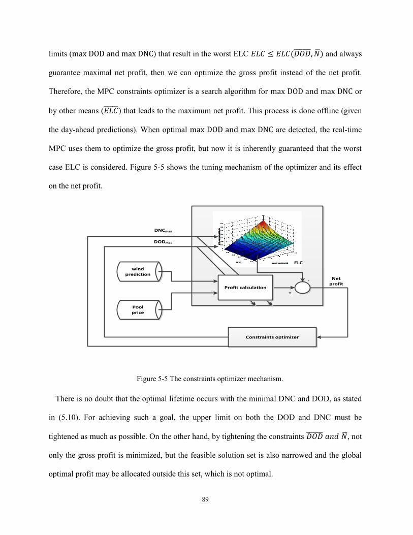
89
limits (max DOD and max DNC) that result in the worst ELC 𝐸𝐿𝐶 ≤ 𝐸𝐿𝐶(𝐷𝑂𝐷 , ��) and always
guarantee maximal net profit, then we can optimize the gross profit instead of the net profit.
Therefore, the MPC constraints optimizer is a search algorithm for max DOD and max DNC or
by other means (𝐸𝐿𝐶 ) that leads to the maximum net profit. This process is done offline (given
the day-ahead predictions). When optimal max DOD and max DNC are detected, the real-time
MPC uses them to optimize the gross profit, but now it is inherently guaranteed that the worst
case ELC is considered. Figure 5-5 shows the tuning mechanism of the optimizer and its effect
on the net profit.
Constraints optimizer
windprediction
Pool price
Net profit
DNCmax
DODmax
-
ELC
+Profit calculation
Figure 5-5 The constraints optimizer mechanism.
There is no doubt that the optimal lifetime occurs with the minimal DNC and DOD, as stated
in (5.10). For achieving such a goal, the upper limit on both the DOD and DNC must be
tightened as much as possible. On the other hand, by tightening the constraints 𝐷𝑂𝐷 𝑎𝑛𝑑 ��, not
only the gross profit is minimized, but the feasible solution set is also narrowed and the global
optimal profit may be allocated outside this set, which is not optimal.

90
This chapter proposes an MPC constraints optimizer for both 𝐷𝑂𝐷 𝑎𝑛𝑑 �� that continues
tightening the constraints as long as the gross profit reduction is less than the expended-life cost.
In other words, the optimizer is a profit-oriented trainer for the constraints that aims at detecting
the constraints that maximize the net profit; these constraints are used later in the real-time
MPC. At each iteration, the optimizer fixes the DNC and DOD constraints and measures the net
profit. Second, it changes one of the constraints and reads the new net profit; the gradient of the
net profit surface guides the optimizer to the direction of the optimal constraints over the
permissible constraints plain. Assuming that the optimal constraints set 𝜓𝑜𝑝𝑡 belongs to a 2D
plain composed of 2 sets (ℕ,𝔻):
𝐷𝑂𝐷 𝑜𝑝𝑡𝜖𝔻,𝔻 = [𝐷𝑂𝐷
𝑚𝑖𝑛, 𝐷𝑂𝐷 𝑚𝑎𝑥]
��𝑜𝑝𝑡𝜖ℕ,ℕ = [��𝑚𝑖𝑛, ��𝑚𝑎𝑥]
𝜓𝑜𝑝𝑡 = (��𝑜𝑝𝑡, 𝐷𝑂𝐷 𝑜𝑝𝑡) = 𝜓(𝑚𝑎𝑥 (𝑁𝐸𝑇. 𝑃𝑅𝑂))
(5.39)
(5.40)
(5.41)
The constraints optimizer detects 𝜓𝑜𝑝𝑡 via this two-stage algorithm (A, B). These stages
represent the offline training that is repeated daily as soon as the day-ahead market prices are
announced.
5.4.4 Constraints Optimizer Algorithm
Stage A (Detecting ��𝑜𝑝𝑡)
1. At k=T0=0; given the predictions 𝕔(𝑘), 𝕦𝑑(𝑘), and the battery initial SOC0; set 𝜓 =
(��𝑚𝑎𝑥, 𝐷𝑂𝐷 𝑚𝑎𝑥).
2. Calculate the storage cost by calculating 𝑆𝐶 in (5.18). Solve the MPC problem (𝜆) in
(5.38) to find the gross profit. By calculating the corresponding ELC from (5.12), the net
profit is reachable as in (5.29).

91
3. Skip to step (8) if ��𝑜𝑝𝑡 is reached; otherwise continue.
4. If this is the first ith iteration, then skip to step (7), otherwise continue.
5. If the problem is feasible, and 𝑖 ≤ 𝑖𝑚𝑎𝑥, 𝑖𝑚𝑎𝑥 = ��𝑚𝑎𝑥, go to step (6). Otherwise, either
�� = 0 or the problem is stuck at an infeasible solution. In both cases, the previous choice
is the best available one (��𝑜𝑝𝑡 = ��(𝑖 − 1)), then stage B is initiated.
6. Calculate the difference in the net profit, if this difference is positive, we skip to step (7);
this means that tightening the DNC improves the net profit. On the other hand, if the
difference is negative, then the previous solution provides the maximum net profit, and set
(��𝑜𝑝𝑡 = ��(𝑖 − 1)) then skip to stage B (go to step 8).
7. Tighten the DNC constraints as follows: ��(𝑖) = ��(𝑖) − 1, update the constraints set 𝜓𝑖𝑗,
then jump to step (2)
Stage B (spotting max optimal 𝐷𝑂𝐷 𝑜𝑝𝑡)
8. Set the MPC constraints at 𝜓 = (��𝑜𝑝𝑡, 𝐷𝑂𝐷 𝑚𝑎𝑥), back to step (2).
9. If this is the first jth iteration, then skip to step (12), otherwise continue.
10. If the problem is feasible, and 𝑗 ≤ 𝑗𝑚𝑎𝑥 ( 𝑗𝑚𝑎𝑥 =𝐷𝑂𝐷 𝑚𝑎𝑥−𝐷𝑂𝐷 𝑚𝑖𝑛
𝛼, where 𝛼 is the 𝐷𝑂𝐷
search sensitivity (resolution)), go to step (11). Otherwise, the algorithm reached 𝐷𝑂𝐷 =
𝐷𝑂𝐷 𝑚𝑖𝑛 or it is stuck at an infeasible solution and, in both cases, the previous choice is the
best available one (𝐷𝑂𝐷 𝑜𝑝𝑡 = 𝐷𝑂𝐷 (𝑗 − 1)) and 𝜓𝑜𝑝𝑡 is reached.
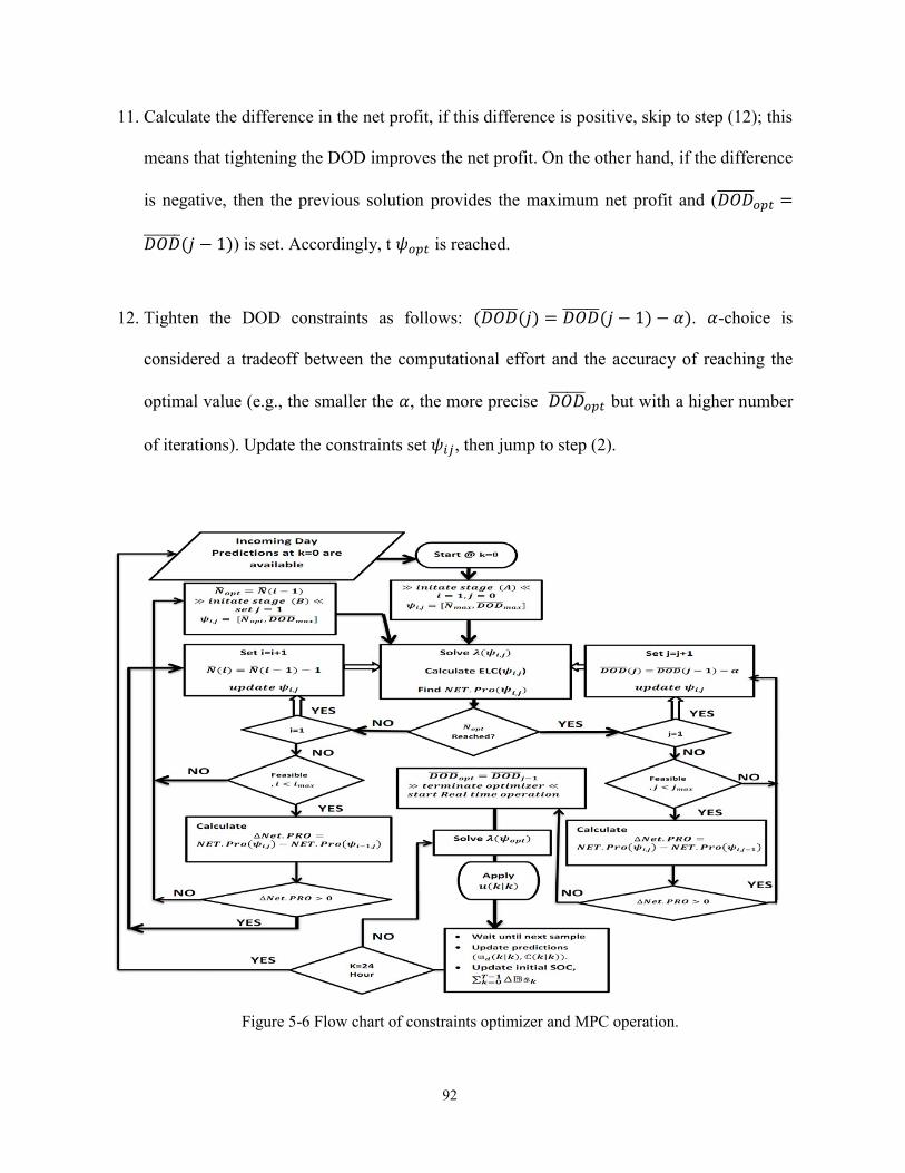
92
11. Calculate the difference in the net profit, if this difference is positive, skip to step (12); this
means that tightening the DOD improves the net profit. On the other hand, if the difference
is negative, then the previous solution provides the maximum net profit and (𝐷𝑂𝐷 𝑜𝑝𝑡 =
𝐷𝑂𝐷 (𝑗 − 1)) is set. Accordingly, t 𝜓𝑜𝑝𝑡 is reached.
12. Tighten the DOD constraints as follows: (𝐷𝑂𝐷 (𝑗) = 𝐷𝑂𝐷 (𝑗 − 1) − 𝛼). 𝛼-choice is
considered a tradeoff between the computational effort and the accuracy of reaching the
optimal value (e.g., the smaller the 𝛼, the more precise 𝐷𝑂𝐷 𝑜𝑝𝑡 but with a higher number
of iterations). Update the constraints set 𝜓𝑖𝑗, then jump to step (2).
Figure 5-6 Flow chart of constraints optimizer and MPC operation.

93
As discussed earlier, the search for the optimal constraints is like the search for the co-
ordinations of the set 𝜓𝑜𝑝𝑡 in a 2D space. Stage A represents a vertical search for ��𝑜𝑝𝑡. While
��𝑜𝑝𝑡 is detected, Stage B is initiated by adopting a horizontal search for 𝐷𝑂𝐷 𝑜𝑝𝑡. Once 𝜓𝑜𝑝𝑡 is
reached, it is used to initiate the real-time MPC that enforces the optimal constraints 𝜆(𝜓𝑜𝑝𝑡).
Real-Time Operation
To deal with disturbance changes (prediction error in the wind and market data), in each
new sample, the MPC is applied with the pre-tuned constraints (𝜓𝑜𝑝𝑡) and the receding control
policy is applied as follows. The new predictions for market and wind data are first updated;
these data have less prediction error as they are short-term forecasts. At each new sample k, the
prediction horizon is decided such that it finishes at the end of the day; (e.g., 𝑛𝑝 =24∗60∗60
𝑇𝑠− 𝐾
) where 𝑇𝑠 is in seconds. Knowing the initial number of changes from charge to discharge ∆𝔹𝕤
already done from the day start (∑𝑇𝑘=−
01 ∆𝔹𝕤𝑘) and the current SOC, the MPC updates its
initial conditions and manages to keep the desired optimal operation (𝜓𝑜𝑝𝑡) until the end of the
day (k=24 hr). The flowchart in Figure 5-6 explains the MPC constraints optimizer.
The optimality of the MPC constraints optimizer is guaranteed as both the ELC and gross
profit are monotonically increasing functions in DNC and DOD. Thus, the resulting net profit
surface (which is the difference between the ELC and gross profit) has a single maximum that
can be easily detected by the proposed searching technique, without being trapped in the local
optimum. Another big concern is the constraints optimizer robustness. In other words, how
much the wind and pool price prediction errors will affect the optimizer decisions. Actually,
with a reasonable prediction error (e.g., 10–15%), it is found that the optimizer has low
sensitivity to such uncertainty.

94
5.5 Case study: Alberta Electricity Market
This study simulates a 5.0 MW WECS connected with 1.0 MW / 3.0 MWh BESS, as shown
in Figure 5-1, in Alberta, Canada. The BESS rating is chosen to be 20% of the WECS power
[122], the capacity is chosen to store up to the rated BESS power for up to three hours. With a
series (2.135 V – 500 Ah) battery, the BESS bank consists of 562 in 5 parallel strings to get the
desired rated capacity; the system has a 1200 voltage dc-link [36]. With the sample time chosen
as one hour because the pool price provided by Alberta Electric System Operator (AESO) is the
average hourly price [125]. In this work, an agreement between the market participant (system
owner) and the grid operator (here; AESO) of updating the market predictions hourly is
assumed; however, the system owner can adjust the sample time to adapt to the existing update
rate of the prediction data as provided by the grid operator. At the end of the day, the system
owner is paid the difference between the generation and consumption by the system operator
according to each hour price.
Further, the prediction horizon (equals the control horizon) is taken for the next 24 hours. As
a result, the problem 𝜆 is solved 24 times a day as long as new pool prices, wind power
predictions and initial conditions are updated at each sample. The battery maximum DOD is
70% to achieve 3200 total number of cycles/life whereas the maximum DNC is set to 4
cycles/day in the constraints optimizer.
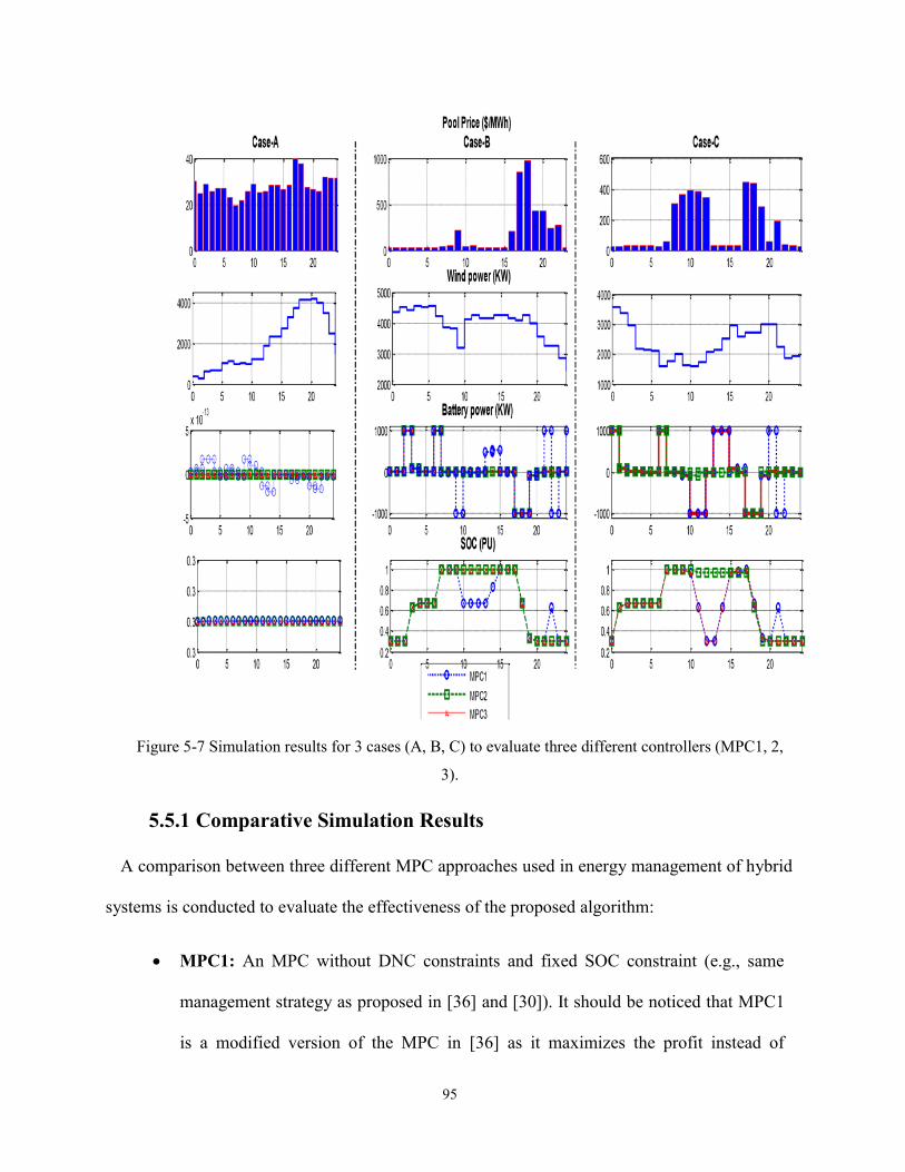
95
Figure 5-7 Simulation results for 3 cases (A, B, C) to evaluate three different controllers (MPC1, 2,
3).
5.5.1 Comparative Simulation Results
A comparison between three different MPC approaches used in energy management of hybrid
systems is conducted to evaluate the effectiveness of the proposed algorithm:
MPC1: An MPC without DNC constraints and fixed SOC constraint (e.g., same
management strategy as proposed in [36] and [30]). It should be noticed that MPC1
is a modified version of the MPC in [36] as it maximizes the profit instead of
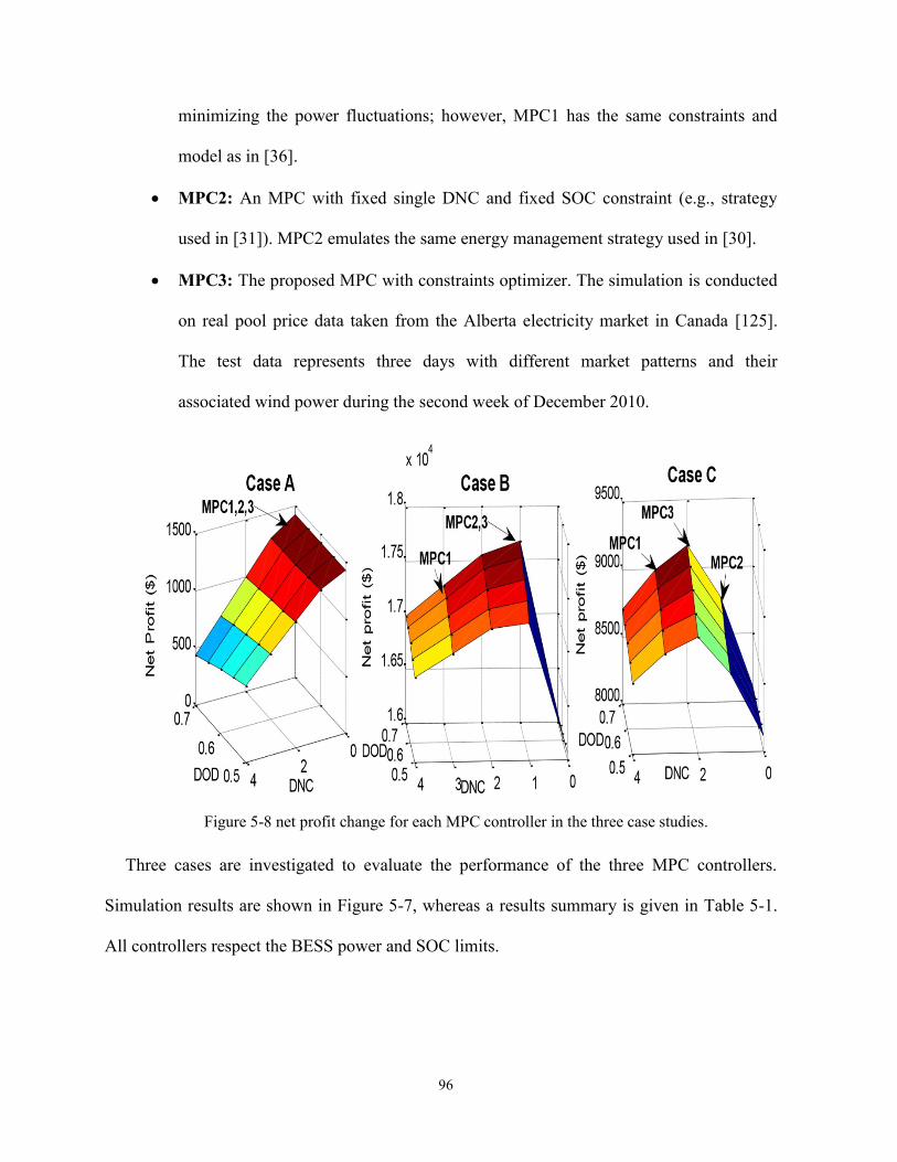
96
minimizing the power fluctuations; however, MPC1 has the same constraints and
model as in [36].
MPC2: An MPC with fixed single DNC and fixed SOC constraint (e.g., strategy
used in [31]). MPC2 emulates the same energy management strategy used in [30].
MPC3: The proposed MPC with constraints optimizer. The simulation is conducted
on real pool price data taken from the Alberta electricity market in Canada [125].
The test data represents three days with different market patterns and their
associated wind power during the second week of December 2010.
Figure 5-8 net profit change for each MPC controller in the three case studies.
Three cases are investigated to evaluate the performance of the three MPC controllers.
Simulation results are shown in Figure 5-7, whereas a results summary is given in Table 5-1.
All controllers respect the BESS power and SOC limits.

97
Table 5-1 Simulation Results.
MPC1 MPC2 MPC3
Case A DNC 0 0 0
Net-profit ($) 1,420$ 1,420$ 1,420$
Case B DNC 3 1 1
Net-profit ($) 17,276.8$ 17,678.2$ 17,678.2$
Case C DNC 3 1 2
Net-profit ($) 8,992$ 8,777.7$ 9,167$
Case A: This case represents a flat market profile with a low maximum to minimum pool
price ratio. The performance of all controllers is the same in this case.
All controllers have decided to stop BESS operation (DNC=0) as the market revenue cannot
cover the operation cost.
Case B: This case represents a single-peak market pattern; however, there is a smaller peak
for just a single hour at t=8. MPC1 targets the maximum profit without considering the ELC.
Thus, it charges the battery three times and achieves the minimum net profit because it has a
large ELC. On the other hand, MPC2 is constrained by a maximum daily single cycle, which
luckily fits that market pattern. As a result, it achieves the maximum net profit. Finally, MPC3
is manipulated by the constraints optimizer that detects the maximum net profit at a single
cycle. The constraints optimizer has compared the revenue of discharging at the small peak at

98
t=8; however, the revenue does not cover the cost of the extra cycle. Thus, the optimal DNC is
chosen as one.
Case C: This is a double-peak market pattern. For MPC1, blinded from the DNC cost, it
detects a fake maximum profit with three cycles. On the contrary, MPC2 is limited by the
maximum single cycle constraint. As a result, it reaches a local maximum profit less than the
profit associated with two cycles. Finally, MPC3 is guided again by the constraints optimizer
which has achieved the maximum net profit of the three controllers (4.4% greater than MPC2,
2% higher than MPC1). Figure 5-8 shows the net profit surface versus the DNC and DOD.
Considering the computational effort, the constraints optimizer computational time is
suitable for the sampling time. It is found that the average iteration time for solving the MPC
problem 𝜆 using MATLAB is 0.486 s on a 3.3 GHz-6 core processor; then the maximum
iterations time equals 𝑖𝑚𝑎𝑥 ∗ 𝑗𝑚𝑎𝑥 ∗ 0.486. In our case, with 𝛼 = 0.01 and ��𝑚𝑎𝑥 = 4, the
maximum time is about 136 s, which is about 4% from the sampling time.
5.5.2 Constraints Optimizer Sensitivity to Prediction Error
This study compares the behavior of the constraints optimizer to gauge its sensitivity to pool
price and wind prediction errors. Two cases are compared. The first assumes a 1-hr sampled
data, whereas the second case assumes the same set sampled at 15-min. The inter-samples
error range is 30%, as shown in Figure 5-9.
Table 5-2 Optimizer results in two different sample times.
Net Profit ��= 1 ��= 2 ��𝑜𝑝𝑡
𝑇𝑠= 60 𝑚𝑖𝑛 17,678$ 17,077$ 1
𝑇𝑠= 15 𝑚𝑖𝑛 17,409$ 16,836$ 1
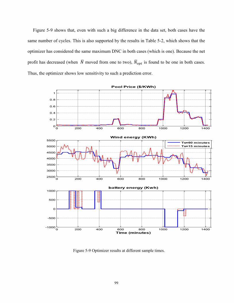
99
Figure 5-9 shows that, even with such a big difference in the data set, both cases have the
same number of cycles. This is also supported by the results in Table 5-2, which shows that the
optimizer has considered the same maximum DNC in both cases (which is one). Because the net
profit has decreased (when �� moved from one to two), ��𝑜𝑝𝑡 is found to be one in both cases.
Thus, the optimizer shows low sensitivity to such a prediction error.
Figure 5-9 Optimizer results at different sample times.

100
5.6 Conclusions
This chapter addressed the development of a comprehensive market-oriented EMS via MPC
for a hybrid power system (WECS with BESS). The MPC aimed at maximizing the daily profit
by dispatching the BESS. The real-time optimization process was based on receiving the
market price and wind power predictions in each new sample. For expanding the BESS
lifetime, constraints on the power rating, the DOD and the DNC were included. The MPC
constraints optimizer tightened the DNC and DOD constraints to achieve the maximum profit
with the minimal expended-lifetime cost. Real wind power and market data of the Alberta
province showed that the proposed MPC constraints optimizer had reached the optimal profit
with the minimal sacrifices in the BESS life. Comparison with other two MPC techniques
showed that the proposed MPC always managed to achieve the maximum net profit for the
system owner.
101
Chapter 6
6 EMS of a Hybrid Wind – Flywheel Energy Storage System via
Model Predictive Control
6.1 Introduction
The maximum power and power ramp rate are important grid codes for renewable energy
resources (e.g., wind farms) in transmission systems. The RES power curtailment regulates the
RES maximum power and ramp rate; however, adding an energy storage system (ESS) can
time shift surplus wind energy instead of curtailing it. The flywheel energy storage system
(FESS) has the advantages of high efficiency and long lifetime; however, it has non-negligible
standby losses and its lifetime is reduced exponentially as the rotating speed increases.
Considering such practical constraints, this chapter presents an EMS for a hybrid power system
composed of a wind farm with a FESS. The FESS time shifts the surplus wind energy to
respect the grid codes and reduce wind curtailment; meanwhile, the EMS aims at minimizing
the FESS standby losses and boosting its lifetime using the predicted wind power data.
The proposed EMS is composed of two cascaded controllers. The first controller is a linear
model predictive controller that defines the long-term FESS power set-point. The second
controller is a real-time adaptive hysteresis controller that compensates for the wind power
prediction error. Simulation results showed that the proposed EMS manages to minimize the
losses significantly as compared to a conventional EMS. Further, a hardware-in-the-loop test is
used to validate the results in a real-time environment. The contributions of this study to the
research field are:

102
• Designing a multi-objective MPC-based algorithm that aims at maximizing the power
imported from the hybrid system to the grid under typical grid code constraints while
reducing FESS losses and boosting its lifetime.
• Converting the MPC optimization problem from a mixed-integer nonlinear programming
(MINLP) problem into a convex one with global optimum and guaranteed feasibility; the
latter is more suitable for real-time control and optimization without loss of accuracy.
• Developing an adaptive online hysteresis controller that is tuned by the MPC algorithm
to compensate for the prediction error; therefore, a robust MPC optimization with
robustness against prediction error is yielded.
• The proposed two-stage EMS is a multi-sample-rate algorithm that serves the
optimization goals while compensating inter-samples and predictions errors.
6.2 Problem Formulation
This work aims at designing an EMS for a hybrid system composed of a large wind farm
with a FESS. The hybrid system must respect the grid code regarding the maximum output
power and its rate. Instead of an excessive wind curtailment, a FESS facilitates short-term
storage for this energy to increase the hybrid system generation while respecting the grid code.
The wind turbines are controlled via a maximum power point tracking (MPPT) algorithm to
harvest the maximum wind power. Assuming an ideal MPPT and a zero pitch angle, the steady-
state wind turbine power is calculated as follows [111]:
𝑃𝑤(𝑡) = 0.5 𝜂𝑊𝜌𝑐𝑝(𝜆𝑜)𝐴𝑣𝑤(𝑡)3 (6.1)
where 𝑃𝑤 , 𝑡, 𝜂𝑊, 𝜌, 𝑐𝑝, 𝜆𝑜 , 𝐴, 𝑉𝑤 are the WECS harvested electrical power, time index, WECS
efficiency (including shaft and gears, generator, power converter and cables efficiencies), air
103
density, power coefficient, optimal tip speed ratio, rotor disk area and the effective wind speed
across the rotor disk, respectively.
Many transmission system operators (TSOs) demand the WECS owners to commit in
advance a maximum generated power (𝑃𝑤(𝑡)), with a rate (∆𝑃𝑤). This commitment is updated
periodically depending on the market. For example, in Alberta-Canada, the WECS owner
updates the maximum power to the TSO every 20 minutes [120]. Other markets, such as the
Spanish market [30], require an advance commitment and impose a penalty as well in case of
violation. The power transferred to the grid according to the grid code (𝑃𝑔𝑐(𝑡)) is
𝑃𝑔𝑐(𝑡) = {𝑃𝑤(𝑡)|𝑃𝑤(𝑡) ≤ ��𝑤(𝑡), −∆��𝑤 ≤ ∆𝑃𝑤(𝑡) ≤ ∆��𝑤 }
∆𝑃𝑤(𝑡) = 𝑃𝑤(𝑡) − 𝑃𝑤(𝑡 − 1)
(6.2)
(6.3)
As given in (6.2)-(6.3), the wind power magnitude and rate are limited by the grid code
regulations [126]. The power curtailment is used to achieve this target by limiting the up-ramp
rate and maximum magnitude. Extra energy is exported from the grid in case of sudden wind
power drop. The curtailed power is calculated as:
𝑃𝑐(𝑡) = 𝑃𝑔𝑐(𝑡) − 𝑃𝑤(𝑡) (6.4)
An effective way to reduce 𝑃𝑐(𝑡) is to add a FESS. An EMS controls the FESS active power
set-point as shown in Figure 6-1. A conventional EMS defines both the curtailed wind power
and the FESS active power, given the wind generation as follows:
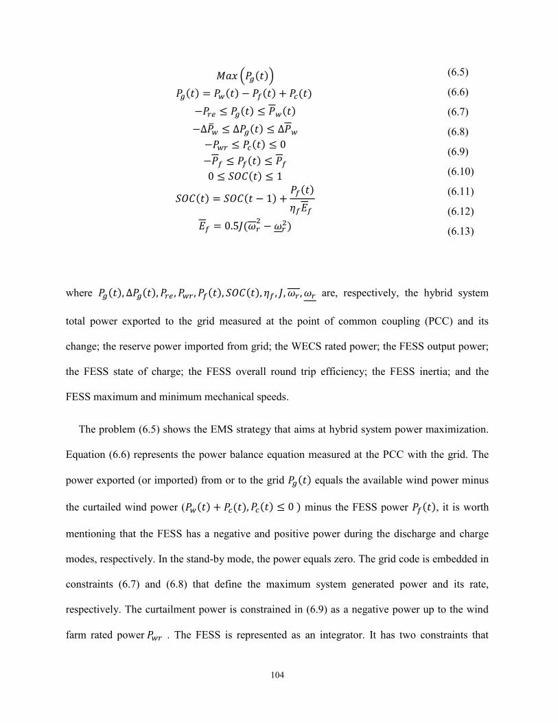
104
𝑀𝑎𝑥 (𝑃𝑔(𝑡))
𝑃𝑔(𝑡) = 𝑃𝑤(𝑡) − 𝑃𝑓(𝑡) + 𝑃𝑐(𝑡)
−𝑃𝑟𝑒 ≤ 𝑃𝑔(𝑡) ≤ 𝑃𝑤(𝑡)
−∆��𝑤 ≤ ∆𝑃𝑔(𝑡) ≤ ∆𝑃𝑤−𝑃𝑤𝑟 ≤ 𝑃𝑐(𝑡) ≤ 0
−𝑃𝑓 ≤ 𝑃𝑓(𝑡) ≤ 𝑃𝑓0 ≤ 𝑆𝑂𝐶(𝑡) ≤ 1
𝑆𝑂𝐶(𝑡) = 𝑆𝑂𝐶(𝑡 − 1) +𝑃𝑓(𝑡)
𝜂𝑓𝐸𝑓
𝐸𝑓 = 0.5𝐽(𝜔𝑟2− 𝜔𝑟
2)
(6.5)
(6.6)
(6.7)
(6.8)
(6.9)
(6.10)
(6.11)
(6.12)
(6.13)
where 𝑃𝑔(𝑡), ∆𝑃𝑔(𝑡), 𝑃𝑟𝑒 , 𝑃𝑤𝑟 , 𝑃𝑓(𝑡), 𝑆𝑂𝐶(𝑡), 𝜂𝑓 , 𝐽, 𝜔𝑟 , 𝜔𝑟 are, respectively, the hybrid system
total power exported to the grid measured at the point of common coupling (PCC) and its
change; the reserve power imported from grid; the WECS rated power; the FESS output power;
the FESS state of charge; the FESS overall round trip efficiency; the FESS inertia; and the
FESS maximum and minimum mechanical speeds.
The problem (6.5) shows the EMS strategy that aims at hybrid system power maximization.
Equation (6.6) represents the power balance equation measured at the PCC with the grid. The
power exported (or imported) from or to the grid 𝑃𝑔(𝑡) equals the available wind power minus
the curtailed wind power (𝑃𝑤(𝑡) + 𝑃𝑐(𝑡), 𝑃𝑐(𝑡) ≤ 0 ) minus the FESS power 𝑃𝑓(𝑡), it is worth
mentioning that the FESS has a negative and positive power during the discharge and charge
modes, respectively. In the stand-by mode, the power equals zero. The grid code is embedded in
constraints (6.7) and (6.8) that define the maximum system generated power and its rate,
respectively. The curtailment power is constrained in (6.9) as a negative power up to the wind
farm rated power 𝑃𝑤𝑟 . The FESS is represented as an integrator. It has two constraints that

105
represent the power limits in (6.10) and the state-of-charge (SOC) in (6.11). The SOC is the
integration of the per-unit power as given in (6.12) taking into consideration the FESS
efficiency 𝜂𝑓 (including converter and cables losses), whereas (6.13) calculates the FESS rated
capacity 𝐸𝑓 that depends on the FESS inertia (J) and the FESS maximum and minimum
mechanical speeds (𝜔𝑟 , 𝜔𝑟). Problem (6.5) charges the FESS up to its limits when wind power
exceeds the constraints (6.7) and (6.8). On the other hand, it fully discharges the FESS when the
wind power is less than the expected value. It is a linear programming problem (LP) that can be
easily solved online in a real-time fashion (with a sample time in the range of seconds);
however, it does not take into consideration the following points:
1- minimizing the standby losses of the FESS;
2- utilizing the knowledge of predicted short-term wind speed in the management decisions
to improve the overall hybrid system performance;
3- taking into consideration the FESS number of cycles as the FESS life is affected
significantly by its operating speed.
This chapter presents an improved EMS that considers these points. To address these
problems, a detailed model for the FESS is required.
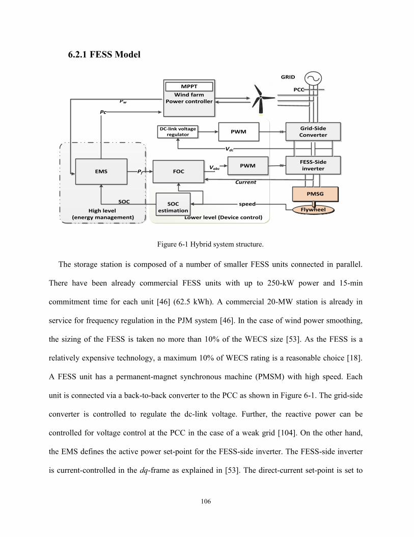
106
6.2.1 FESS Model
Wind farmPower controller
EMS FOCPWM
FESS-Sideinverter
Pf
speedFlywheel
PMSG
GRID
SOC
High level (energy management) Lower level (Device control)
SOCestimation
Grid-SideConverter
MPPT
Pc
PCC
Pw
DC-link voltage regulator
Vabc
Current
Vdc
PWM
Figure 6-1 Hybrid system structure.
The storage station is composed of a number of smaller FESS units connected in parallel.
There have been already commercial FESS units with up to 250-kW power and 15-min
commitment time for each unit [46] (62.5 kWh). A commercial 20-MW station is already in
service for frequency regulation in the PJM system [46]. In the case of wind power smoothing,
the sizing of the FESS is taken no more than 10% of the WECS size [53]. As the FESS is a
relatively expensive technology, a maximum 10% of WECS rating is a reasonable choice [18].
A FESS unit has a permanent-magnet synchronous machine (PMSM) with high speed. Each
unit is connected via a back-to-back converter to the PCC as shown in Figure 6-1. The grid-side
converter is controlled to regulate the dc-link voltage. Further, the reactive power can be
controlled for voltage control at the PCC in the case of a weak grid [104]. On the other hand,
the EMS defines the active power set-point for the FESS-side inverter. The FESS-side inverter
is current-controlled in the dq-frame as explained in [53]. The direct-current set-point is set to

107
zero to reduce losses [104], while the quadrature current set-point is controlled to manipulate
the electric torque as follows:
𝑇𝑒∗ =
3
2
𝑝
2𝜓𝑝𝑚𝑖𝑠𝑞
∗ =𝑃𝑓∗
𝜔𝑟
(6.14)
where 𝑇𝑒 , 𝑝, 𝜓𝑝𝑚, 𝑖𝑠𝑞∗ , 𝑃𝑓
∗, 𝜔𝑟 are the FESS electric torque set-point; PMSM number of pole pairs;
PMSM flux and the stator quadrature current set-point; the FESS power set-point; and the FESS
mechanical speed, respectively. The current controller is a proportional-integral (PI) controller
that defines a quadrature stator voltage set-point. A pulse-width modulation (PWM) scheme
embeds the voltage set-point into switching pulses for the inverter. Neglecting the fast inverter
switching dynamics, the inverter acts as an amplifier with a gain equals half the dc-link voltage.
Further details are given in [104]. Since this work focuses on EMS that works with a sample
time in range of several seconds, all the current closed-loop dynamics is modeled as a low-pass
filter [27] as expressed in (6.15).
𝐼𝑠𝑞(𝑠) =𝐼𝑠𝑞
∗(𝑠)
𝜏𝑖𝑠 + 1
(6.15)
where 𝐼𝑠𝑞 , 𝑠, 𝜏𝑖 are the stator quadrature current; Laplace transform variable; and the time-
constant of the closed-loop current control dynamics. The electric torque manipulates the
machine mechanical speed according to the following shaft dynamic equation [53] as given in
(6.16).
𝑇𝑒(𝑠) − 𝑇𝑙(𝑠)
𝜔𝑟(𝑠)=
1
𝐽𝑠 + 𝐵
(6.16)
where 𝐵, 𝑇𝑙 are the friction and mechanical torque, respectively. The output power (𝑃𝑓) is the
deference between the air-gap power (𝑃𝑔𝑎𝑏) and the power loss (𝑃𝑙𝑜𝑠𝑠) [53]. It is worth
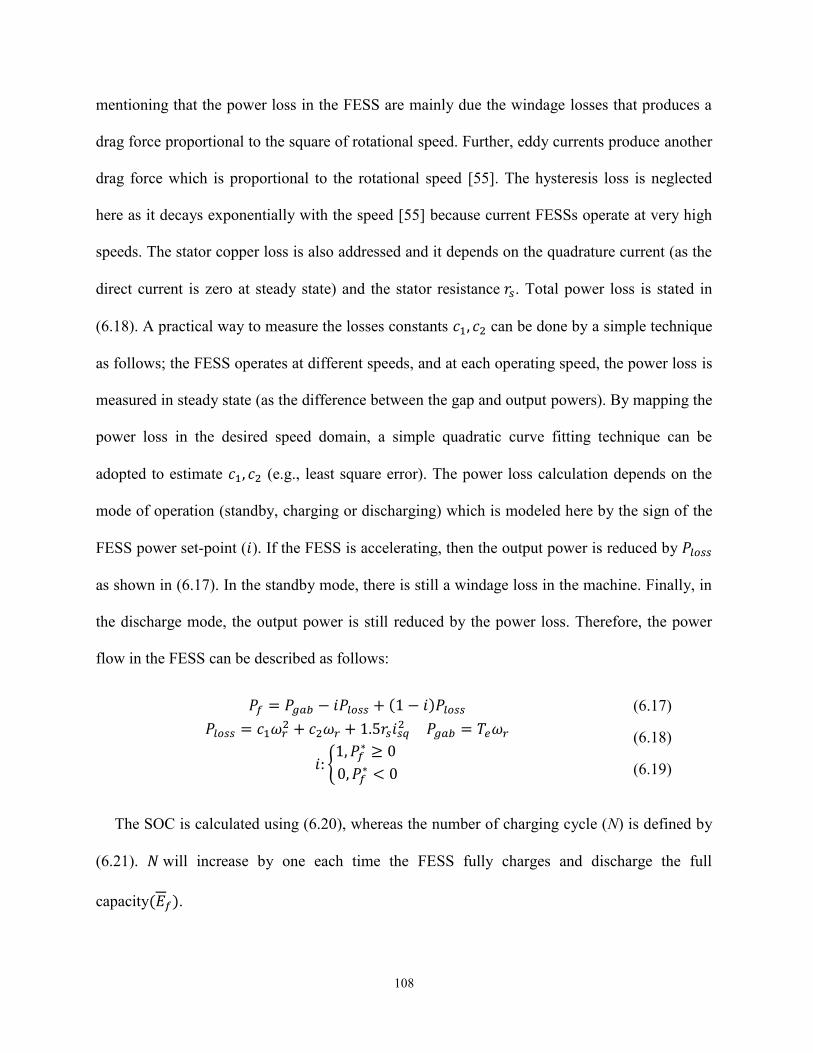
108
mentioning that the power loss in the FESS are mainly due the windage losses that produces a
drag force proportional to the square of rotational speed. Further, eddy currents produce another
drag force which is proportional to the rotational speed [55]. The hysteresis loss is neglected
here as it decays exponentially with the speed [55] because current FESSs operate at very high
speeds. The stator copper loss is also addressed and it depends on the quadrature current (as the
direct current is zero at steady state) and the stator resistance 𝑟𝑠. Total power loss is stated in
(6.18). A practical way to measure the losses constants 𝑐1, 𝑐2 can be done by a simple technique
as follows; the FESS operates at different speeds, and at each operating speed, the power loss is
measured in steady state (as the difference between the gap and output powers). By mapping the
power loss in the desired speed domain, a simple quadratic curve fitting technique can be
adopted to estimate 𝑐1, 𝑐2 (e.g., least square error). The power loss calculation depends on the
mode of operation (standby, charging or discharging) which is modeled here by the sign of the
FESS power set-point (𝑖). If the FESS is accelerating, then the output power is reduced by 𝑃𝑙𝑜𝑠𝑠
as shown in (6.17). In the standby mode, there is still a windage loss in the machine. Finally, in
the discharge mode, the output power is still reduced by the power loss. Therefore, the power
flow in the FESS can be described as follows:
𝑃𝑓 = 𝑃𝑔𝑎𝑏 − 𝑖𝑃𝑙𝑜𝑠𝑠 + (1 − 𝑖)𝑃𝑙𝑜𝑠𝑠
𝑃𝑙𝑜𝑠𝑠 = 𝑐1𝜔𝑟2 + 𝑐2𝜔𝑟 + 1.5𝑟𝑠𝑖𝑠𝑞
2 𝑃𝑔𝑎𝑏 = 𝑇𝑒𝜔𝑟
𝑖: {1, 𝑃𝑓
∗ ≥ 0
0, 𝑃𝑓∗ < 0
(6.17)
(6.18)
(6.19)
The SOC is calculated using (6.20), whereas the number of charging cycle (N) is defined by
(6.21). 𝑁 will increase by one each time the FESS fully charges and discharge the full
capacity(𝐸𝑓).
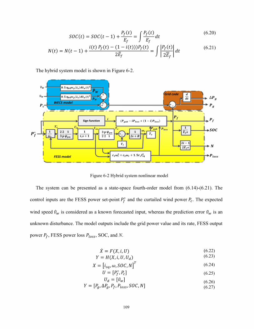
109
𝑆𝑂𝐶(𝑡) = 𝑆𝑂𝐶(𝑡 − 1) +𝑃𝑓(𝑡)
𝐸𝑓 = ∫
𝑃𝑓(𝑡)
𝐸𝑓 𝑑𝑡
𝑁(𝑡) = 𝑁(𝑡 − 1) +𝑖(𝑡) 𝑃𝑓(𝑡) − (1 − 𝑖(𝑡)))𝑃𝑓(𝑡)
2��𝑓= ∫|
𝑃𝑓(𝑡)
2𝐸𝑓| 𝑑𝑡
(6.20)
(6.21)
The hybrid system model is shown in Figure 6-2.
Sign function
𝟏
𝝎𝒓
𝟐
𝟑
𝟐
𝒑
𝟏
𝝍𝒑𝒎
𝟏
𝝉𝒊𝒔 + 𝟏
𝟑
𝟐
𝒑
𝟐
𝝍𝒑𝒎
𝟏
𝟏
𝑱𝒔 + 𝑩
𝑻𝒆
𝒄𝟏𝝎𝒓𝟐 + 𝒄𝟐𝝎𝒓 + 𝟏.𝟓𝒓𝒔𝑰𝒔𝒒
𝟐
(𝑷𝒈𝒂𝒃 − 𝒊𝑷𝒍𝒐𝒔𝒔 + (𝟏 − 𝒊)𝑷𝒍𝒐𝒔𝒔)
𝟏
��𝒇𝒔
𝟐𝒊 − 𝟏
𝟐��𝒇𝒔
𝑻𝒍
𝒅
𝒅𝒕
𝑷 𝑾
��𝑾
𝑷𝒄
𝑷𝒇∗
∆𝑷𝒈
𝑷𝒈
𝑷𝒇
𝑺𝑶𝑪
𝑵
𝑷𝒍𝒐𝒔𝒔
+ +
+ +
+ −
+ −
𝑻𝒆∗ 𝑰𝒔𝒒
∗ 𝑰𝒔𝒒 𝑻𝒆 𝝎𝒓
𝑷𝒈𝒂𝒃 𝑷𝒍𝒐𝒔𝒔
𝒊 𝑷𝒇
WECS model
𝒗 𝑾 𝟎.𝟓 𝜼𝑾𝝆𝒄𝒑(𝝀𝒐)𝑨𝒗 𝒘(𝒕)𝟑
𝟎.𝟓 𝜼𝑾𝝆𝒄𝒑(𝝀𝒐)𝑨𝒗 𝒘(𝒕)𝟑 𝒗 𝑾
FESS model
Grid code
Figure 6-2 Hybrid system nonlinear model
The system can be presented as a state-space fourth-order model from (6.14)-(6.21). The
control inputs are the FESS power set-point 𝑃𝑓∗ and the curtailed wind power 𝑃𝑐. The expected
wind speed 𝑣𝑤 is considered as a known forecasted input, whereas the prediction error ��𝑤 is an
unknown disturbance. The model outputs include the grid power value and its rate, FESS output
power 𝑃𝑓, FESS power loss 𝑃𝑙𝑜𝑠𝑠, SOC, and N.
�� = 𝐹(𝑋, 𝑖, 𝑈)𝑌 = 𝐻(𝑋, 𝑖, 𝑈, 𝑈𝑑)
𝑋 = [𝑖𝑠𝑞 , 𝜔, 𝑆𝑂𝐶,𝑁]𝑇
𝑈 = [𝑃𝑓∗, 𝑃𝑐]
𝑈𝑑 = [��𝑤]𝑌 = [𝑃𝑔, ∆𝑃𝑔, 𝑃𝑓 , 𝑃𝑙𝑜𝑠𝑠, 𝑆𝑂𝐶, 𝑁]
(6.22)
(6.23)
(6.24)
(6.25)
(6.26)
(6.27)

110
6.2.2 The Proposed Control Structure
To utilize the knowledge of future expected wind speed ��𝑤, a finite-horizon model
predictive controller is used to optimize the future controlled inputs 𝑃𝑓∗, 𝑃𝑐 according to a certain
objective function. Because the maximum wind power is updated each commitment
period 𝑇𝑐𝑜𝑚, the prediction horizon is chosen as 𝑛𝑝 = 𝑇𝑐𝑜𝑚
𝑇𝑠1 where 𝑇𝑠1 is the sampling time of
the expected wind speed. 𝑇𝑠1 is in the range of minutes to provide a long prediction period with
low number of samples. Now, the operational control problem can formulated as
𝑀𝑖𝑛 (𝛼∑ 𝑃𝑙𝑜𝑠𝑠(𝑘𝑇𝑠1)𝑛𝑝
𝑘=1−∑ 𝑃𝑔(𝑘𝑇𝑠1)
𝑛𝑝
𝑘=1)
𝑋(𝑘𝑇𝑠1 + 𝑇𝑠1) = 𝐹(𝑋(𝑘𝑇𝑠1), 𝑖(𝑘𝑇𝑠1), 𝑈(𝑘𝑇𝑠1), 𝑈𝑑(𝑘𝑇𝑠1))
𝑌(𝑘𝑇𝑠1) = 𝐻(𝑋(𝑘𝑇𝑠1), 𝑖(𝑘𝑇𝑠1), 𝑈(𝑘𝑇𝑠1), 𝑈𝑑(𝑘𝑇𝑠1))
𝑌(𝐾𝑇𝑠1) ≤ 𝑌
{
𝑃𝑟𝑒 ≤ 𝑃𝑔(𝑘𝑇𝑠1) ≤ 𝑃𝑤(𝑇𝑐𝑜𝑚)
−∆𝑃𝑤 ≤ ∆𝑃𝑔(𝑘𝑇𝑠1) ≤ ∆𝑃𝑤0 ≤ 𝑆𝑂𝐶(𝑘𝑇𝑠1) ≤ 1
𝑁(𝑇𝑐𝑜𝑚) ≤ 𝑛
𝑈(𝐾𝑇𝑠1) ≤ 𝑈 {−𝑃𝑓 ≤ 𝑃𝑓
∗(𝑘𝑇𝑠1) ≤ 𝑃𝑓−𝑃𝑤𝑟 ≤ 𝑃𝑐(𝑘𝑇𝑠1) ≤ 0
𝑣𝑤(𝑘𝑇𝑠1) ⊆ [𝑣𝑤(𝑗𝑇𝑠2), 𝑣𝑤(𝑗𝑇𝑠2 + 𝑆𝑅)], 𝑆𝑅 =𝑇𝑠1𝑇𝑠2
, 𝑗 = 𝑘×𝑆𝑅 ∀𝑘
(6.28)
(6.29)
(6.30)
(6.31)
(6.32)
(6.33)
(6.34)
(6.35)
(6.36)
(6.37)
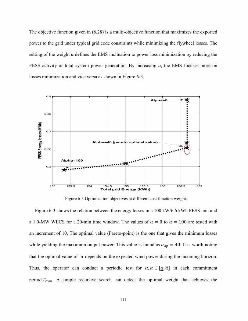
111
The objective function given in (6.28) is a multi-objective function that maximizes the exported
power to the grid under typical grid code constraints while minimizing the flywheel losses. The
setting of the weight α defines the EMS inclination to power loss minimization by reducing the
FESS activity or total system power generation. By increasing α, the EMS focuses more on
losses minimization and vice versa as shown in Figure 6-3.
Figure 6-3 Optimization objectives at different cost function weight.
Figure 6-3 shows the relation between the energy losses in a 100 kW/6.6 kWh FESS unit and
a 1.0-MW WECS for a 20-min time window. The values of 𝛼 = 0 to 𝛼 = 100 are tested with
an increment of 10. The optimal value (Pareto-point) is the one that gives the minimum losses
while yielding the maximum output power. This value is found as 𝛼𝑜𝑝 = 40. It is worth noting
that the optimal value of 𝛼 depends on the expected wind power during the incoming horizon.
Thus, the operator can conduct a periodic test for 𝛼, 𝛼 ∈ [𝛼, 𝛼] in each commitment
period 𝑇𝑐𝑜𝑚. A simple recursive search can detect the optimal weight that achieves the
153 153.5 154 154.5 155 155.5 156 156.5 157
0.2
0.25
0.3
0.35
0.4
Total grid Energy (KWh)
FESS
Ene
rgy
loss
es (K
Wh)
Alpha=0
Alpha=100
Alpha=40 (pareto optimal value)

112
maximum exported power such that the losses is minimal or 𝛼𝑜𝑝 = {𝛼 ∈ [𝛼, 𝛼]|{��𝑔|𝑃𝑙𝑜𝑠𝑠}}.
Another simpler suboptimal technique is that the operator makes a constant choice for 𝛼 that
reflects the operator’s preferences for power minimization.
The state-space model is discretized with a sampling time Ts1 as given in (6.29), (6.30). The
inequalities (6.31)-(6.34) represent the output constraints whereas (6.35)-(6.36) are the input
constraints. In (6.31), the power exported to the grid is upper bounded by the maximum WECS
power committed with the grid at this time (Tcom), and the down limit is the maximum allowed
grid support in case of wind down-ramp that cannot be handled by the FESS. Equation (6.32)
defines the grid code rising and falling power ramp rates. The SOC limits are given by (6.33),
and the number of cycles at the end of the commitment period is given by (6.34). The FESS
power constraint is expressed by (6.35). Finally, the curtailed wind power is defined as a
negative power up to the rated WECS Pwr as given by (6.36). The optimization problem (6.28)
is a nonconvex problem that is solved in this work by two model modifications. First, the
nonlinear state-space model converts the optimization into a nonlinear mixed integer problem
that faces feasibility problems and has no guaranteed global minimum. This problem is solved
later in this chapter by converting the system into a time-variant linear model without loss of
accuracy. Second, the wind speed data has a prediction error which affects the results optimality
(that is why many works do not include weather forecasts in EMS decisions, e.g., [127]).
Further, the predicted wind speed data is discretized using a large sample rate (e.g., 5 minutes);
in reality, the wind speed changes significantly during this time window. Equation (6.37)
models this change as the wind speed 𝑣𝑤(𝑘𝑇𝑠1) is defined as a set of wind speeds during the
same time window if a smaller sample time 𝑇𝑠2 is considered (e.g., 1 s). In other words,
[𝑣𝑤(𝑗𝑇𝑠2), 𝑣𝑤(𝑗𝑇𝑠2 + 𝑆𝑅)] is the inter-samples wind speed set during the bigger time window

113
𝑘𝑇𝑠1, where SR is defined as the sample times ratio. Such uncertainty-related problems are
addressed by a faster online adaptive hysteresis controller
6.3 The Proposed Control Algorithm
6.3.1 Hybrid System Linearization
To convert the optimization problem into a convex one suitable for online operational
control, a linear state-space model is required. The nonlinear model has an integer state
represented by the sign of the FESS operation mode. To obtain a linear model, the integer state
is converted to a constant, and then a time-variant linearized model is driven. The integer state
(i) depends on the absolute value of (𝑃𝑓∗) as given in (6.19). To find a constant integer that
indicates the FESS mode of operation, the following approach is proposed. It is known that the
FESS is only allowed to operate in the charge mode when the wind power is greater than the
maximum allowable power. On the contrary, the FESS is allowed to operate in the discharge
mode when the expected generated wind power is below the maximum grid power. As a result,
the relation between the expected wind power and the maximum one (both known for the
incoming horizon) gives a sufficient relation to identify the FESS operating mode, and in such a
case, the integer variable i is generated as in (6.38). equation (6.38) models the FESS state as a
charging when the expected wind power is higher than the maximum power, and vice versa.
𝑖(𝑡): {1, ��𝑤(𝑡) ≥ 𝑃𝑤(𝑡)
0, 𝑃𝑤(𝑡) < 𝑃𝑤(𝑡)
(6.38)
Now, a linear model of (6.22) and (6.23) can be reached by linearizing the power loss
relation in (6.18). The system identification technique is adopted for this purpose because it is
practical, reliable and accurate modeling method [128].
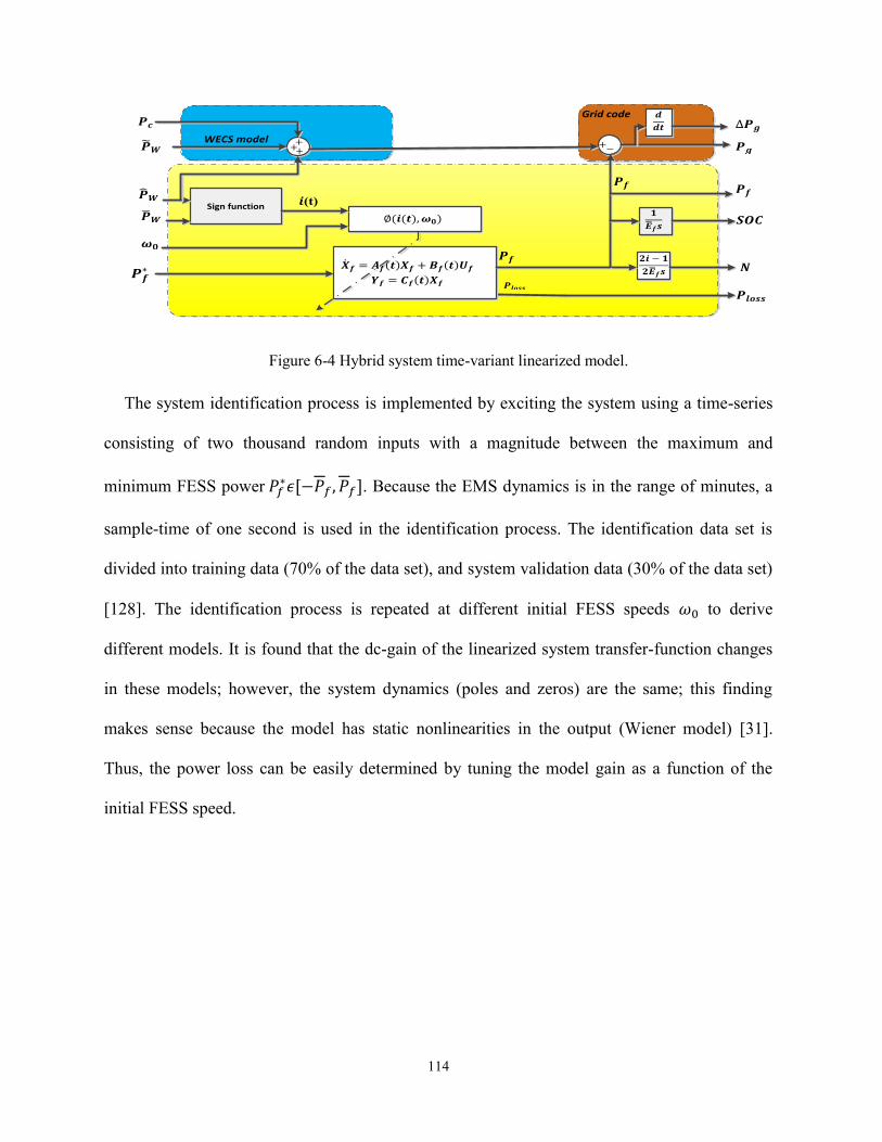
114
Sign function
𝟏
��𝒇𝒔
𝒅
𝒅𝒕
��𝑾
𝑷𝒄
𝑷𝒇∗
∆𝑷𝒈
𝑷𝒈
𝑷𝒇
𝑺𝑶𝑪
𝑵
𝑷𝒍𝒐𝒔𝒔
+ + +
−
𝑷𝒍𝒐𝒔𝒔
𝑷𝒇
𝝎𝟎
𝑷 𝑾
��𝑾 ∅(𝒊(𝒕),𝝎𝟎)
+
𝑷𝒇
𝒊(t)
𝟐𝒊 − 𝟏
𝟐��𝒇𝒔
WECS model
Grid code
��𝒇 = 𝑨𝒇(𝒕)𝑿𝒇 + 𝑩𝒇(𝒕)𝑼𝒇
𝒀𝒇 = 𝑪𝒇(𝒕)𝑿𝒇
Figure 6-4 Hybrid system time-variant linearized model.
The system identification process is implemented by exciting the system using a time-series
consisting of two thousand random inputs with a magnitude between the maximum and
minimum FESS power 𝑃𝑓∗𝜖[−𝑃𝑓 , 𝑃𝑓]. Because the EMS dynamics is in the range of minutes, a
sample-time of one second is used in the identification process. The identification data set is
divided into training data (70% of the data set), and system validation data (30% of the data set)
[128]. The identification process is repeated at different initial FESS speeds 𝜔0 to derive
different models. It is found that the dc-gain of the linearized system transfer-function changes
in these models; however, the system dynamics (poles and zeros) are the same; this finding
makes sense because the model has static nonlinearities in the output (Wiener model) [31].
Thus, the power loss can be easily determined by tuning the model gain as a function of the
initial FESS speed.
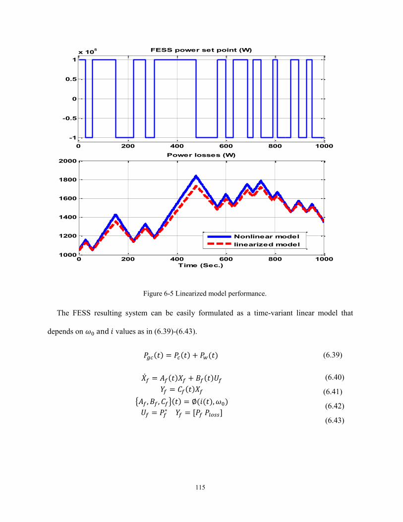
115
Figure 6-5 Linearized model performance.
The FESS resulting system can be easily formulated as a time-variant linear model that
depends on 𝜔0 and 𝑖 values as in (6.39)-(6.43).
𝑃𝑔𝑐(𝑡) = 𝑃𝑐(𝑡) + 𝑃𝑤(𝑡) (6.39)
��𝑓 = 𝐴𝑓(𝑡)𝑋𝑓 + 𝐵𝑓(𝑡)𝑈𝑓𝑌𝑓 = 𝐶𝑓(𝑡)𝑋𝑓
{𝐴𝑓 , 𝐵𝑓, 𝐶𝑓}(𝑡) = ∅(𝑖(𝑡),𝜔0)
𝑈𝑓 = 𝑃𝑓∗ 𝑌𝑓 = [𝑃𝑓 𝑃𝑙𝑜𝑠𝑠]
(6.40)
(6.41)
(6.42)
(6.43)
0 200 400 600 800 1000
-1
-0.5
0
0.5
1
x 105 FESS power set point (W)
0 200 400 600 800 10001000
1200
1400
1600
1800
2000
Time (Sec.)
Power losses (W)
Nonlinear model
linearized model

116
where ∅ is a look-up table array that generates the system linearized model depending on the
mode of operation and initial speed. By considering the wind power instead of the wind speed,
the overall system can be expressed as a linear model as shown in Figure 6-4. By comparing
different identification models performances, it is found that a third-order model gives the best
fitting with a fitting accuracy of 93.1%. Figure 6-5 compares the results of the linearized model
(6.40) and the nonlinear model (6.22). After augmenting the other linear states with the
linearized FESS model, a complete state-space model is reached.
The linearized model converts the MPC into a convex problem as shown by (6.44). First,
given the expected and maximum WECS power, np linearized models are calculated for each
sample in the coming horizon as shown by (6.45), (6.46). Further, the prediction error is
assumed zero as this error is compensated by a faster controller that will be explained later.
Because the MPC control action compensates for the expected disturbance ��𝑤, the generated
MPC set-points are designated as follows 𝑈 = [��𝑓∗, ��𝑐]. Further modifications for the input
constraints are also considered, where the curtailment is only allowed if the expected WECS
power is greater than the maximum as given by (6.54). The FESS is allowed to charge in case of
over maximum WECS power and vice versa; however, it can operate in the standby mode in
both cases as expressed in (6.51),(6.52).
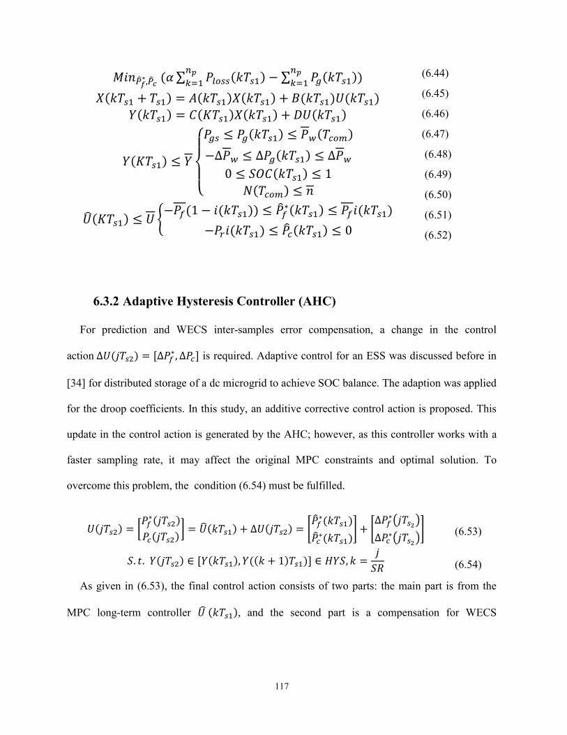
117
𝑀𝑖𝑛��𝑓∗,��𝑐
(𝛼 ∑ 𝑃𝑙𝑜𝑠𝑠(𝑘𝑇𝑠1)𝑛𝑝𝑘=1
− ∑ 𝑃𝑔(𝑘𝑇𝑠1)𝑛𝑝𝑘=1
)
𝑋(𝑘𝑇𝑠1 + 𝑇𝑠1) = 𝐴(𝑘𝑇𝑠1)𝑋(𝑘𝑇𝑠1) + 𝐵(𝑘𝑇𝑠1)𝑈(𝑘𝑇𝑠1)
𝑌(𝑘𝑇𝑠1) = 𝐶(𝐾𝑇𝑠1)𝑋(𝑘𝑇𝑠1) + 𝐷𝑈(𝑘𝑇𝑠1)
𝑌(𝐾𝑇𝑠1) ≤ 𝑌
{
𝑃𝑔𝑠 ≤ 𝑃𝑔(𝑘𝑇𝑠1) ≤ 𝑃𝑤(𝑇𝑐𝑜𝑚)
−∆𝑃𝑤 ≤ ∆𝑃𝑔(𝑘𝑇𝑠1) ≤ ∆𝑃𝑤0 ≤ 𝑆𝑂𝐶(𝑘𝑇𝑠1) ≤ 1
𝑁(𝑇𝑐𝑜𝑚) ≤ 𝑛
𝑈 (𝐾𝑇𝑠1) ≤ 𝑈 {−𝑃𝑓(1 − 𝑖(𝑘𝑇𝑠1)) ≤ ��𝑓
∗(𝑘𝑇𝑠1) ≤ 𝑃𝑓𝑖(𝑘𝑇𝑠1)
−𝑃𝑟𝑖(𝑘𝑇𝑠1) ≤ ��𝑐(𝑘𝑇𝑠1) ≤ 0
(6.44)
(6.45)
(6.46)
(6.47)
(6.48)
(6.49)
(6.50)
(6.51)
(6.52)
6.3.2 Adaptive Hysteresis Controller (AHC)
For prediction and WECS inter-samples error compensation, a change in the control
action ∆𝑈(𝑗𝑇𝑠2) = [∆𝑃𝑓∗, ∆𝑃𝑐] is required. Adaptive control for an ESS was discussed before in
[34] for distributed storage of a dc microgrid to achieve SOC balance. The adaption was applied
for the droop coefficients. In this study, an additive corrective control action is proposed. This
update in the control action is generated by the AHC; however, as this controller works with a
faster sampling rate, it may affect the original MPC constraints and optimal solution. To
overcome this problem, the condition (6.54) must be fulfilled.
𝑈(𝑗𝑇𝑠2) = [𝑃𝑓∗(𝑗𝑇𝑠2)
𝑃𝑐(𝑗𝑇𝑠2)] = 𝑈 (𝑘𝑇𝑠1) + ∆𝑈(𝑗𝑇𝑠2) = [
��𝑓∗(𝑘𝑇𝑠1)
��𝑐∗(𝑘𝑇𝑠1)
] + [∆𝑃𝑓
∗(𝑗𝑇𝑠2)
∆𝑃𝑐∗(𝑗𝑇𝑠2)
]
𝑆. 𝑡. 𝑌(𝑗𝑇𝑠2) ∈ [𝑌(𝑘𝑇𝑠1), 𝑌((𝑘 + 1)𝑇𝑠1)] ∈ 𝐻𝑌𝑆, 𝑘 =𝑗
𝑆𝑅
(6.53)
(6.54)
As given in (6.53), the final control action consists of two parts: the main part is from the
MPC long-term controller 𝑈 (𝑘𝑇𝑠1), and the second part is a compensation for WECS

118
prediction error generated by AHC ∆𝑈(𝑗𝑇𝑠2). In case the compensation error is zero, the
condition (6.54) is always satisfied, and the AHC generates zero.
Condition (6.54) guarantees that the AHC correction will not significantly change the outputs
of process, since the outputs at any intersample 𝑗𝑇𝑠2 should be located between the previous and
next value as expected by the MPC problem (6.44) known here as the hysteresis limits. For
example, at 𝑗𝑇𝑠2 = 630 s (𝑇𝑠2 = 1 s), the AHC can produce a control action such that the
current outputs are within the MPC hysteresis values; 𝑌(𝑗𝑇𝑠2) ∈ [𝑌(10𝑇𝑠1), 𝑌(11𝑇𝑠1)], 𝑇𝑠1 =
1 𝑚𝑖𝑛. If this is not the case, then a different control action is required to bring the current
output within the hysteresis limits again as will be explained later. It is worth mentioning that
the hysteresis can be given some flexibility which means that the output can diverge slightly
from the optimal solution given by the MPC. This is possible by modifying the condition (6.54)
to be as follows:
𝑌(𝑗𝑇𝑠2) ∈ [𝑌(𝑘𝑇𝑠1) − 𝜆, 𝑌((𝑘 + 1)𝑇𝑠1) + 𝜆] ∈ 𝐻𝑌𝑆(𝑘𝑇𝑠1) (6.55)
As noticed, the output is allowed to diverge outside the optimal MPC solution by a tolerance
(𝜆). The next step is how to design the AHC that guarantees that 𝑌 ∈ 𝐻𝑌𝑆.This section is
composed of two parts. First, Section 6.3.3 investigates different uncertainty modes and
how ∆𝑈(𝑗𝑇𝑠2) is calculated. Second, Section 6.3.4 discusses how the AHC satisfies the MPC
constraints by fulfilling (6.54).
6.3.3 Uncertainty Modes
The actual wind power can have six different positions, defined here as six modes if
compared to the expected value of wind power 𝑃𝑤(𝑡) and the maximum wind power 𝑃𝑤(𝑡) as
shown in Figure 6-6.
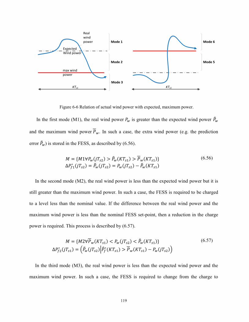
119
KTs1 KTs1
Real wind power
ExpectedWind power
max wind power
Mode 2
Mode 1
Mode 3
Mode 5
Mode 6
Figure 6-6 Relation of actual wind power with expected, maximum power.
In the first mode (M1), the real wind power 𝑃𝑤 is greater than the expected wind power ��𝑤
and the maximum wind power 𝑃𝑤. In such a case, the extra wind power (e.g. the prediction
error ��𝑤) is stored in the FESS, as described by (6.56).
𝑀 = {𝑀1∀𝑃𝑤(𝑗𝑇𝑠2) > ��𝑤(𝐾𝑇𝑠1) > 𝑃𝑤(𝐾𝑇𝑠1)}
∆𝑃𝑓1∗ (𝑗𝑇𝑠2) = ��𝑤(𝑗𝑇𝑠2) = 𝑃𝑤(𝑗𝑇𝑠2) − ��𝑤(𝐾𝑇𝑠1)
(6.56)
In the second mode (M2), the real wind power is less than the expected wind power but it is
still greater than the maximum wind power. In such a case, the FESS is required to be charged
to a level less than the nominal value. If the difference between the real wind power and the
maximum wind power is less than the nominal FESS set-point, then a reduction in the charge
power is required. This process is described by (6.57).
𝑀 = {𝑀2∀𝑃𝑤(𝐾𝑇𝑠1) < 𝑃𝑤(𝑗𝑇𝑠2) < ��𝑤(𝐾𝑇𝑠1)}
∆𝑃𝑓2∗ (𝑗𝑇𝑠1) = (��𝑤(𝑗𝑇𝑠2)|��𝑓
∗(𝐾𝑇𝑠1) > 𝑃𝑤(𝐾𝑇𝑠1) − 𝑃𝑤(𝑗𝑇𝑠2))
(6.57)
In the third mode (M3), the real wind power is less than the expected wind power and the
maximum wind power. In such a case, the FESS is required to change from the charge to

120
discharge mode till the total hybrid system power is maximum. This process is described by
(6.58).
𝑀 = {𝑀3∀𝑃𝑤(𝐾𝑇𝑠1) < 𝑃𝑤(𝐾𝑇𝑠1) < ��𝑤(𝐾𝑇𝑠1)}
∆𝑃𝑓3∗ (𝑗𝑇𝑠2) = −��𝑓
∗(𝑘𝑇𝑠1) − [𝑃𝑤(𝐾𝑇𝑠1) − 𝑃𝑤(𝑗𝑇𝑠2)]
(6.58)
In the fourth mode (M4), the real wind power is less than the expected wind power and the
maximum wind power. In this case, the expected wind power is less than the maximum wind
power. Thus, the FESS is in the discharge mode. In M4, The FESS can discharge more till the
hybrid system power reaches its maximum. This process is described by (6.59).
𝑀 = {𝑀4∀𝑃𝑤(𝑗𝑇𝑠2) < ��𝑤(𝐾𝑇𝑠1) < 𝑃𝑤(𝐾𝑇𝑠1)}
∆𝑃𝑓4∗ (𝐾𝑇𝑠2) = ��𝑤(𝑗𝑇𝑠2)
(6.59)
In the fifth mode (M5), the real wind power is less than the maximum wind power but more
than the expected wind power. In this case, the expected wind power is less than the maximum
wind power. Thus, the FESS is in the discharge mode. In M5, The FESS can discharge less till
the hybrid system power reaches its maximum. This process is described by (6.60).
𝑀 = {𝑀5∀��𝑤(𝐾𝑇𝑠1) < 𝑃𝑤(𝑗𝑇𝑠2) < 𝑃𝑤(𝐾𝑇𝑠1)}
∆𝑃𝑓5∗ (𝑗𝑇𝑠2) = (��𝑤(𝑗𝑇𝑠2)|𝑃𝑓
∗(𝐾𝑇𝑠1) < 𝑃𝑤(𝐾𝑇𝑠1) − 𝑃𝑤(𝑗𝑇𝑠2))
(6.60)
Finally, in the sixth mode (M6), the real wind power is more than both the maximum and
expected wind powers. In this case, the expected wind power is less than the maximum wind
power. Thus, the FESS is in the discharge mode. In M6, the FESS changes its mode to charge
the extra wind power. This process is described by (6.61).
𝑀 = {𝑀6∀ 𝑃𝑤(𝑗𝑇𝑆2) > ��𝑤(𝐾𝑇𝑠1) > 𝑃𝑤(𝐾𝑇𝑠1)}
∆𝑃𝑓6∗ (𝑗𝑇𝑠2) = [𝑃𝑤(𝑗𝑇𝑠2) − 𝑃𝑤(𝐾𝑇𝑠1)] − 𝑃𝑓
∗(𝐾𝑇𝑠1)
(6.61)

121
6.3.4 The Two-stage Controller
Only one of modes (6.56)-(6.61) is enabled at any time. The total FESS is calculated and
limited by the FESS thermal limit in (6.35). However, ∆𝑃𝑓∗ may lead to undesired changes in the
controlled outputs Y. It is very important to make sure that the outputs will be within the
predefined limits determined by the MPC controller to guarantee optimum solution. Generally
speaking, the outputs change ∆𝑌(𝑗𝑇𝑠2) due to the AHC correction ∆𝑃𝑓∗(𝑗𝑇𝑠2) at steady-state
depends on the system dc gain ℍ(𝑘𝑇𝑠1) as in (6.63) which depends on the linearized FESS
model.
∆𝑌(𝑗𝑇𝑠2) = ℍ(𝑘𝑇𝑠1)∆𝑃𝑓∗(𝑗𝑇𝑠2)
ℍ(𝑘𝑇𝑠1) = lim𝑧→1
𝐷(𝑘𝑇𝑠1) + 𝐶(𝑘𝑇𝑠1)(𝑧𝐼 − 𝐴(𝑘𝑇𝑠1))−1𝐵(𝑘𝑇𝑠1)
(6.62)
(6.63)
where A, B, C and D are extracted from (6.42), assuming zero disturbance and I is a unity
matrix. The AHC applies the following rule to guarantee overall system operation within MPC
optimal constraints:
{
𝑌(𝐾𝑇𝑠1) + ∆𝑌(𝑗𝑇𝑠2) > 𝐻𝑌𝑆: {𝑃𝑓(𝑗𝑇𝑠2) = ��𝑓∗(𝑘𝑇𝑠1)
𝑌(𝐾𝑇𝑠1) + ∆𝑌(𝑗𝑇𝑠2)𝜖𝐻𝑌𝑆: {𝑃𝑓(𝑗𝑇𝑠2) = ��𝑓∗(𝑘𝑇𝑠1) + ∆𝑃𝑓
∗(𝑗𝑇𝑠2)∀ℍ
𝑌(𝐾𝑇𝑠1) + ∆𝑌(𝑗𝑇𝑠2) < 𝐻𝑌𝑆: {𝑃𝑓(𝑗𝑇𝑠2) = ��𝑓∗(𝑘𝑇𝑠1),ℍ < 0
(6.64)
The control law (6.64) means that the compensating control action ∆𝑃𝑓∗(𝑗𝑇𝑠2) is applied if
and only if all the resulting controlled outputs are within their allowable domain or hysteresis
limit (𝑌(𝐾𝑇𝑠1) + ∆𝑌(𝑗𝑇𝑠2)𝜖𝐻𝑌𝑆) or if this control action will direct the outputs back to 𝐻𝑌𝑆
depending the output sensitivity to this input. For example, without loss of generality, let us
consider that Y is the SOC and the input is ∆𝑃𝑓∗(𝑗𝑇𝑠2) which has positive sensitivity (positive DC
gain) with respect to the SOC. In case 𝑆𝑂𝐶 < 𝐻𝑌𝑆, the allowed control action is charging to
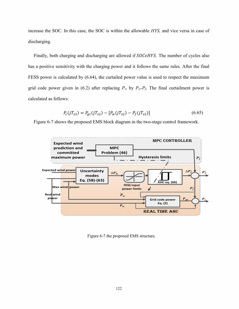
122
increase the SOC. In this case, the SOC is within the allowable HYS, and vice versa in case of
discharging.
Finally, both charging and discharging are allowed if 𝑆𝑂𝐶𝜖𝐻𝑌𝑆. The number of cycles also
has a positive sensitivity with the charging power and it follows the same rules. After the final
FESS power is calculated by (6.64), the curtailed power value is used to respect the maximum
grid code power given in (6.2) after replacing Pw by Pw-Pf. The final curtailment power is
calculated as follows:
𝑃𝑐(𝑗𝑇𝑠2) = 𝑃𝑔𝑐(𝑗𝑇𝑠2) − [𝑃𝑤(𝑗𝑇𝑠2) − 𝑃𝑓(𝑗𝑇𝑠2)] (6.65)
Figure 6-7 shows the proposed EMS block diagram in the two-stage control framework.
MPCProblem (46)
Uncertainty modes
Eq. (58)-(63)
Grid code powerEq. (2)
AHC eq. (66)
Expected wind prediction and
committed maximum power Hysteresis limits
Expected wind power
Max wind power
Real wind power
∆𝑷𝒇𝒊∗
∆𝑷𝒇
∗
𝑷 𝒇∗
𝑷𝒇∗
𝑷𝒇∗
𝑷𝒘
FESS input power limits
𝑷𝒈𝒄 𝑷𝒄
MPC controller
Real time AHC
𝑷𝒘
Figure 6-7 the proposed EMS structure.

123
6.4 Case Study
In this case study, a 150 MW wind farm is participating in the power market in the Alberta
transmission system- Canada. The Alberta system operator (AESO) requires that the wind
facility updates its maximum power limit every 20 minutes. Further, the ramp-rate should not
exceed 10% of the rated plant power per minute [129], [120]. The prediction horizon is taken as
20 minutes (each commitment period). A typical wind speed profile is generated by TurbSim
[130], a wind simulator developed by the National Renewable Energy Laboratory (NREL). A
Great Plains Low-Level Jet (GP-LLJ) turbulence model is used with a mean wind speed of 7
m/s-normal turbulence intensity sampled each 6 seconds [130]. The resulting wind profile is
applied on a doubly-fed induction generator-based wind farm Simulink model developed by
Hydro-Quebec [131]. The resulting wind power profile represents the real wind power profile.
By averaging this profile each 1 minute, the expected wind power is calculated, and this data is
assumed to be known for the MPC. The prediction error is the difference between the real wind
power and this averaged value. Distribution for perdition error is shown in Figure 6-8 for a data
set of 400 samples. As shown in Figure 6-8, the prediction error range is about ∓15%. For the
MPC, the prediction horizon is taken as 𝑇𝑠1 = 60 s, 𝑛𝑝 = 20, when the AHC works at a sample
rate 𝑇𝑠2 = 6 s.
A 15 MW/1 MWh FESS station is added to the system which is composed of 100 kW units.
To enhance the lifetime of the FESS, it is only allowed to have one cycle each commitment
period 𝑁=1, which means 72 cycle per day. The FESS model parameters are taken from [53]
with a higher inertia as shown in Table 6-1.
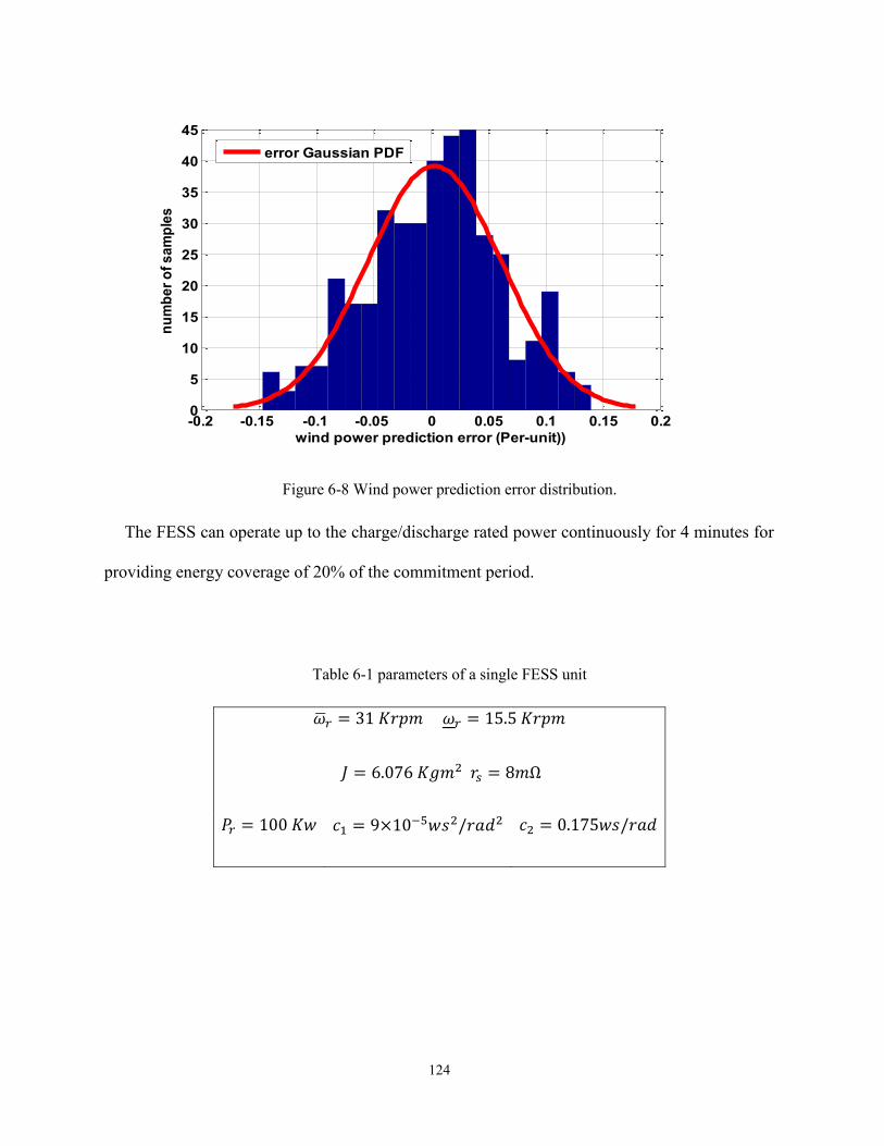
124
Figure 6-8 Wind power prediction error distribution.
The FESS can operate up to the charge/discharge rated power continuously for 4 minutes for
providing energy coverage of 20% of the commitment period.
Table 6-1 parameters of a single FESS unit
��𝑟 = 31 𝐾𝑟𝑝𝑚 𝜔𝑟 = 15.5 𝐾𝑟𝑝𝑚
𝐽 = 6.076 𝐾𝑔𝑚2 𝑟𝑠 = 8𝑚Ω
𝑃𝑟 = 100 𝐾𝑤 𝑐1 = 9×10⁻⁵𝑤𝑠2/𝑟𝑎𝑑2 𝑐2 = 0.175𝑤𝑠/𝑟𝑎𝑑
-0.2 -0.15 -0.1 -0.05 0 0.05 0.1 0.15 0.20
5
10
15
20
25
30
35
40
45
wind power prediction error (Per-unit))
nu
mb
er
of
sa
mp
les
error Gaussian PDF
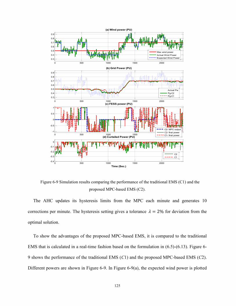
125
Figure 6-9 Simulation results comparing the performance of the traditional EMS (C1) and the
proposed MPC-based EMS (C2).
The AHC updates its hysteresis limits from the MPC each minute and generates 10
corrections per minute. The hysteresis setting gives a tolerance 𝜆 = 2% for deviation from the
optimal solution.
To show the advantages of the proposed MPC-based EMS, it is compared to the traditional
EMS that is calculated in a real-time fashion based on the formulation in (6.5)-(6.13). Figure 6-
9 shows the performance of the traditional EMS (C1) and the proposed MPC-based EMS (C2).
Different powers are shown in Figure 6-9. In Figure 6-9(a), the expected wind power is plotted
0 500 1000 1500 2000
0.3
0.4
0.5
0.6
0.7
0.8
0.9
(a) Wind power (PU)
0 500 1000 1500 2000
0.3
0.4
0.5
0.6
0.7
0.8
0.9
(b) Grid Power (PU)
0 500 1000 1500 2000
-1
-0.5
0
0.5
1
(c) FESS power (PU)
0 500 1000 1500 2000-0.4
-0.3
-0.2
-0.1
0
Time (Sec.)
(d) Curtailed Power (PU)
Max wind power
Actual Wind Power
Expected Wind Power
Actual Pw
Pg-C2
Pg-C1
C2
C1
C2- MPC output
C2- final power
C1- final power

126
by the blue dotted line whereas the maximum WECS is plotted by the red line. The simulation
is conducted for two commitments periods (40 minutes), and actual wind power is measured
each 6 s. It should be noted that the wind power has a high ramp rate at 𝑡 = 1200 s which is
followed by a sudden drop in power. Furthermore, in the first commitment period, the wind has
two peaks exceeding the maximum, typically at 𝑡 = 0 and 300 s. Similarly, in the second
commitment period, two peaks occur at 𝑡 = 1200 and 1800 s. The controller C1 has managed
to maximize the power exported to the grid slightly than the controller C2 as shown in Figure 6-
9(b) during the starting period of the commitment period; however, C2 decided to keep the
FESS idle (standby) during this early period. The main reason for this performance is the
lifetime constraints embedded in C2 where it aims at maximizing the power without over-acting
on the FESS. Figure 6-9(c) shows that the proposed controller (C2) charges the FESS late at 𝑡 =
300 s to discharge this energy back at the wind power gap at 𝑡 = 600 s. On the other hand, the
traditional controller (C1) keeps charging and discharging to regulate the WECS power to the
maximum.
Further, this can be noted in Figure 6-9(d) which shows that the curtailed wind power is
higher in (C2) than (C1) due to the higher activity of the FESS in case of C1. However, this
difference is only 1% regarding the energy exported to the grid.
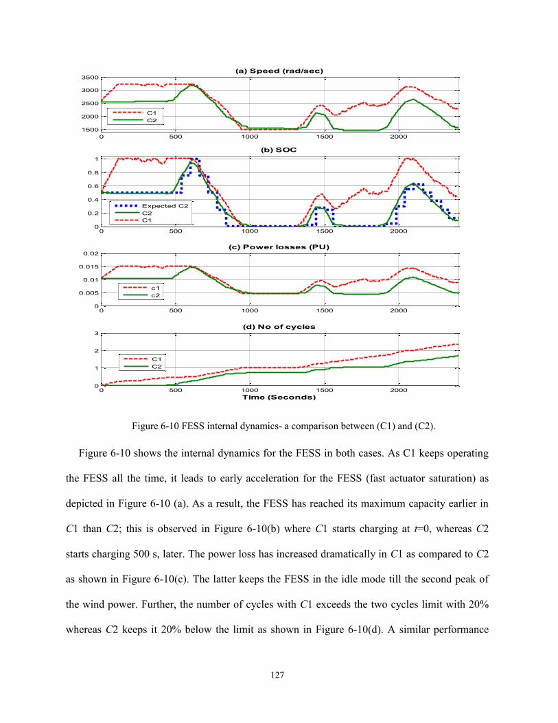
127
Figure 6-10 FESS internal dynamics- a comparison between (C1) and (C2).
Figure 6-10 shows the internal dynamics for the FESS in both cases. As C1 keeps operating
the FESS all the time, it leads to early acceleration for the FESS (fast actuator saturation) as
depicted in Figure 6-10 (a). As a result, the FESS has reached its maximum capacity earlier in
C1 than C2; this is observed in Figure 6-10(b) where C1 starts charging at t=0, whereas C2
starts charging 500 s, later. The power loss has increased dramatically in C1 as compared to C2
as shown in Figure 6-10(c). The latter keeps the FESS in the idle mode till the second peak of
the wind power. Further, the number of cycles with C1 exceeds the two cycles limit with 20%
whereas C2 keeps it 20% below the limit as shown in Figure 6-10(d). A similar performance
0 500 1000 1500 2000
1500
2000
2500
3000
3500
(a) Speed (rad/sec)
0 500 1000 1500 20000
0.2
0.4
0.6
0.8
1
(b) SOC
0 500 1000 1500 20000
0.005
0.01
0.015
0.02
(c) Power losses (PU)
0 500 1000 1500 20000
1
2
3
Time (Seconds)
(d) No of cycles
C1
C2
Expected C2
C2
C1
c1
c2
C1
C2
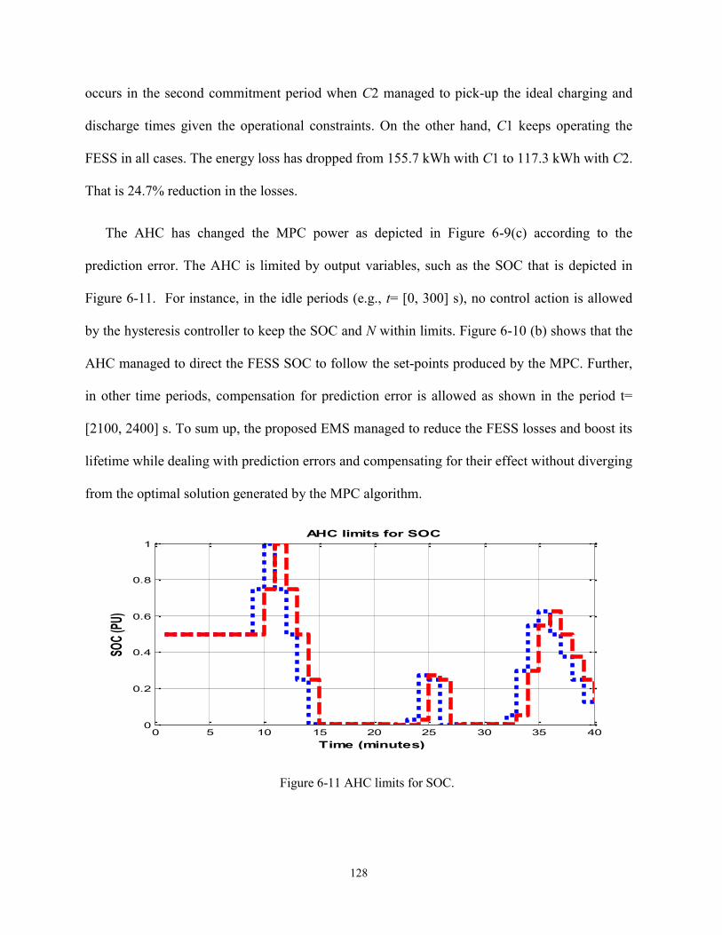
128
occurs in the second commitment period when C2 managed to pick-up the ideal charging and
discharge times given the operational constraints. On the other hand, C1 keeps operating the
FESS in all cases. The energy loss has dropped from 155.7 kWh with C1 to 117.3 kWh with C2.
That is 24.7% reduction in the losses.
The AHC has changed the MPC power as depicted in Figure 6-9(c) according to the
prediction error. The AHC is limited by output variables, such as the SOC that is depicted in
Figure 6-11. For instance, in the idle periods (e.g., t= [0, 300] s), no control action is allowed
by the hysteresis controller to keep the SOC and N within limits. Figure 6-10 (b) shows that the
AHC managed to direct the FESS SOC to follow the set-points produced by the MPC. Further,
in other time periods, compensation for prediction error is allowed as shown in the period t=
[2100, 2400] s. To sum up, the proposed EMS managed to reduce the FESS losses and boost its
lifetime while dealing with prediction errors and compensating for their effect without diverging
from the optimal solution generated by the MPC algorithm.
Figure 6-11 AHC limits for SOC.
0 5 10 15 20 25 30 35 400
0.2
0.4
0.6
0.8
1
Time (minutes)
SOC
(PU)
AHC limits for SOC
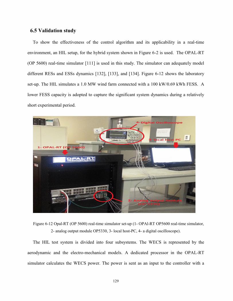
129
6.5 Validation study
To show the effectiveness of the control algorithm and its applicability in a real-time
environment, an HIL setup, for the hybrid system shown in Figure 6-2 is used. The OPAL-RT
(OP 5600) real-time simulator [111] is used in this study. The simulator can adequately model
different RESs and ESSs dynamics [132], [133], and [134]. Figure 6-12 shows the laboratory
set-up. The HIL simulates a 1.0 MW wind farm connected with a 100 kW/0.69 kWh FESS. A
lower FESS capacity is adopted to capture the significant system dynamics during a relatively
short experimental period.
Figure 6-12 Opal-RT (OP 5600) real-time simulator set-up (1- OPAl-RT OP5600 real-time simulator,
2- analog output module OP5330, 3- local host-PC, 4- a digital oscilloscope).
The HIL test system is divided into four subsystems. The WECS is represented by the
aerodynamic and the electro-mechanical models. A dedicated processor in the OPAL-RT
simulator calculates the WECS power. The power is sent as an input to the controller with a
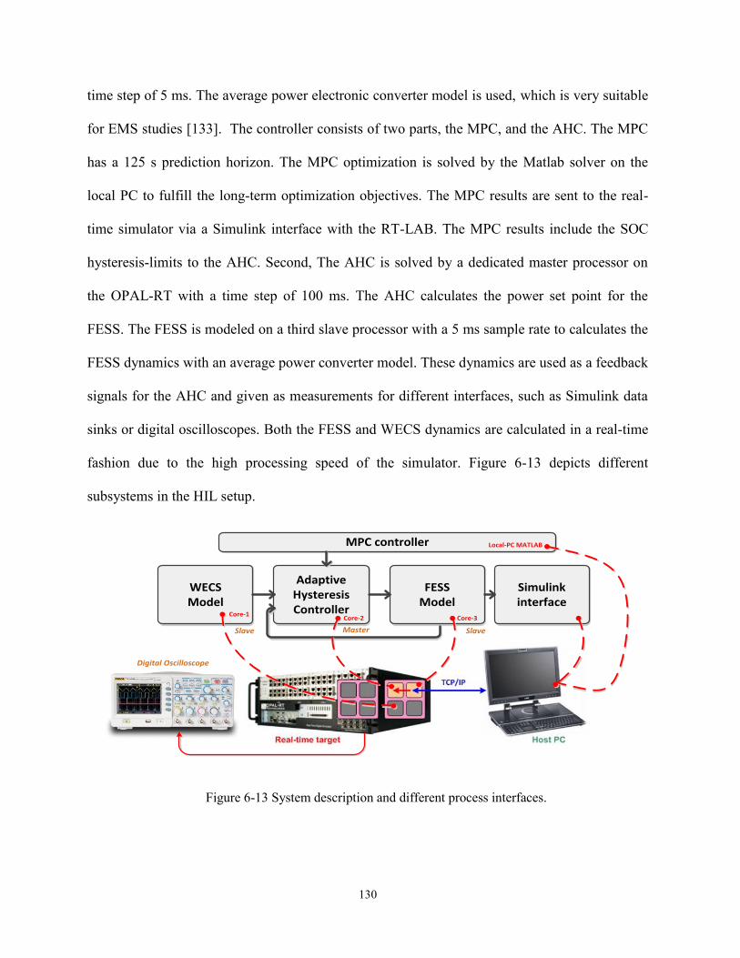
130
time step of 5 ms. The average power electronic converter model is used, which is very suitable
for EMS studies [133]. The controller consists of two parts, the MPC, and the AHC. The MPC
has a 125 s prediction horizon. The MPC optimization is solved by the Matlab solver on the
local PC to fulfill the long-term optimization objectives. The MPC results are sent to the real-
time simulator via a Simulink interface with the RT-LAB. The MPC results include the SOC
hysteresis-limits to the AHC. Second, The AHC is solved by a dedicated master processor on
the OPAL-RT with a time step of 100 ms. The AHC calculates the power set point for the
FESS. The FESS is modeled on a third slave processor with a 5 ms sample rate to calculates the
FESS dynamics with an average power converter model. These dynamics are used as a feedback
signals for the AHC and given as measurements for different interfaces, such as Simulink data
sinks or digital oscilloscopes. Both the FESS and WECS dynamics are calculated in a real-time
fashion due to the high processing speed of the simulator. Figure 6-13 depicts different
subsystems in the HIL setup.
WECSModel
AdaptiveHysteresisController
FESSModel
MPC controller
Simulinkinterface
Local-PC MATLAB
Core-1Core-2 Core-3
MasterSlave Slave
Digital Oscilloscope
Figure 6-13 System description and different process interfaces.

131
The standard vector control scheme is adopted in the PMSM drive system of the FESS,
which facilitates fast control characteristics over the drive system torque. The closed-loop
torque response is dictated by the closed-loop current response. The system responses are
measured by a four-channel digital oscilloscope (Agilent DSOX2004A). Key system variables
are shown in Figure 6-14.
The wind profile generated in a 25-s period as illustrated in figure 6-14(a). The expected and
maximum wind power profiles are also shown in Figure 6-14(a). The output power of the FESS
is provided in Figure 6-14(b). The hysteresis limits for the SOC, which are generated by the
MPC algorithm, are shown in Figure 6-14(c). The hysteresis limits are desired to be bounded
between 𝑆𝑂𝐶𝑚𝑖𝑛, 5% < 𝑆𝑂𝐶𝑚𝑖𝑛 < 7% and 𝑆𝑂𝐶𝑚𝑎𝑥, 20% < 𝑆𝑂𝐶𝑚𝑎𝑥 < 35%, which are
depicted by the red and blue lines in Figure 6-14(c), respectively. The resulting real-time SOC
profile is shown by the green line in Figure 6-14(c). Knowing the SOC limits and the difference
between real and expected wind powers, the AHC generates the FESS power set point in real-
time, which is used to generate the torque command of the PMSM drive system. The resulting
FESS power loss profile is shown in Figure 6-14(d).
As shown in Figure 6-14(b), the wind power starts with a value that it less than the maximum
wind power; i.e., 𝑃𝑤 < 𝑃𝑤. Because the initial SOC lies within the SOC limits, the AHC allows
the FESS to discharge till point (0) where 𝑃𝑤 > 𝑃𝑤. In such a case, the AHC charges the FESS
with this surplus wind power (𝑃𝑤 − 𝑃𝑤). At point (1), the wind power decreases below the
maximum value (𝑃𝑤 < 𝑃𝑤); thus the FESS is discharged till point (2). Although 𝑃𝑤 < 𝑃𝑤, the
AHC prevents further discharge for the FESS to stay inside the SOC limits provided by the
MPC to satisfy the optimization problem in (6.44). The FESS stays in the stand-by mode until a
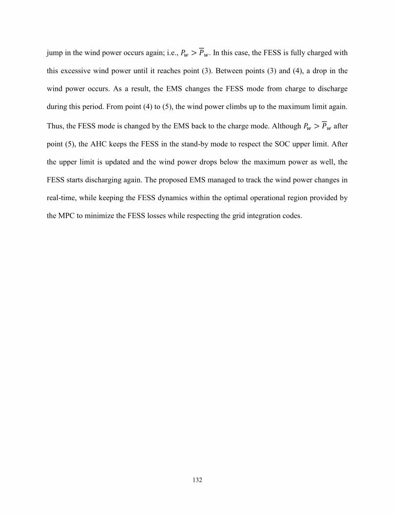
132
jump in the wind power occurs again; i.e., 𝑃𝑤 > 𝑃𝑤. In this case, the FESS is fully charged with
this excessive wind power until it reaches point (3). Between points (3) and (4), a drop in the
wind power occurs. As a result, the EMS changes the FESS mode from charge to discharge
during this period. From point (4) to (5), the wind power climbs up to the maximum limit again.
Thus, the FESS mode is changed by the EMS back to the charge mode. Although 𝑃𝑤 > 𝑃𝑤 after
point (5), the AHC keeps the FESS in the stand-by mode to respect the SOC upper limit. After
the upper limit is updated and the wind power drops below the maximum power as well, the
FESS starts discharging again. The proposed EMS managed to track the wind power changes in
real-time, while keeping the FESS dynamics within the optimal operational region provided by
the MPC to minimize the FESS losses while respecting the grid integration codes.
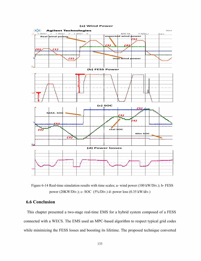
133
(a) Wind Power
(b) FESS Power
(c) SOC
(d) Power losses
Real wind power
max wind power
expected wind power
discharge
Full charge
MAX. SOC
real SOC
Min SOC
(2)
(1)
(3)
(4)
(5)
(0)
(1)
(3) (4)
(5)
(0)
(2)
Figure 6-14 Real-time simulation results with time scales; a- wind power (100 kW/Div.); b- FESS
power (20KW/Div.); c- SOC (5%/Div.) d- power loss (0.35 kW/div.)
6.6 Conclusion
This chapter presented a two-stage real-time EMS for a hybrid system composed of a FESS
connected with a WECS. The EMS used an MPC-based algorithm to respect typical grid codes
while minimizing the FESS losses and boosting its lifetime. The proposed technique converted

134
the MPC optimization problem from a nonlinear mixed integer into a linear convex problem
without loss of accuracy. The AHC realized the second stage. The AHC was tuned by the MPC
to ensure optimum operation under uncertainties associated with wind power perdition errors.
The proposed EMS was compared with a traditional EMS on a typical 150-MW WECS.
Furthermore, the real-time performance of the proposed EMS was validated in an HIL test
bench. The proposed EMS managed to reduce the FESS losses by 25% as compared to the
conventional EMS while compensating for the prediction errors and respecting the grid
integration codes.
.

135
Chapter 7
7 Multi Energy Storage Robust Operation in Active Distribution
Network
7.1 Introduction
This chapter discusses the day-ahead operation of multi ESSs in a distribution system with
RESs. The chapter presents a tool to robustly allocate the allowable operating zones of active
power margins for multi ESSs without violating typical distribution system constraints. This
tool helps ESSs to manage their energy independently without violating the power system
constraints. The main contribution is considering the power uncertainties (loads and renewable
energy) without taking very conservative decisions. For defining robust operating zones (ROZ)
for ESSs; first, a fuzzy expert relaxes the uncertainty domain. Second, a particle swarm
optimization (PSO) algorithm detects the worst-case power uncertainty. Finally, the ROZ for
each ESS that maintains safe system operation limits (voltage limits and branches ampacity) is
obtained.
7.2 Problem Formulation
The typical energy management problem for any ESS ES is as follows:
Max𝑝𝑠𝑘
(𝔽(𝑝𝑘𝐸𝑆))
𝑠. 𝑡. {𝜃 𝑘+1𝐸𝑆 = 𝕊(𝜃𝑘
𝐸𝑆, 𝑝𝑘𝐸𝑆), ‖𝜃𝑘
𝐸𝑆‖ ≤ 𝜃𝑘𝐸𝑆
0 = 𝜙𝑘(𝑝𝑘𝐸𝑆, 𝜃𝑘
𝑔, ℙ𝑒𝑥), ‖𝜃𝑘
𝑔‖ ≤ 𝜃𝑘
𝑔
, 𝐸𝑆𝜖𝒩𝑠, 𝑘𝜖𝒩𝑘
(7.1)
(7.2)
(7.3)

136
As shown in (7.1), the ESS aims at optimizing a certain cost function 𝔽(𝑝𝑘𝐸𝑆) which can be
the ESS owner profit maximization by means like energy arbitrage, load shifting or even
renewable energy integration [3]. Optimizing 𝔽(𝑝𝑘𝐸𝑆) depends on choosing the optimal future
ESS dispatch power 𝑝𝑠𝑘. The future horizon can be minutes, hours, or even days. Without the
loss of generality, we assume day-ahead operation example. The optimization problem has two
constraints sets. First the ESS dynamical model 𝕊(𝜃𝑘𝑔) in (7.2) that includes the storage states
𝜃𝑘𝑔, such as (energy and power level, state of charge (SOC) and number of charging cycles).
Energy storage states are limited in (7.2) (e.g., the state of charge is less than one, and the power
is less than the converter rating). The second model is the grid power flow model 𝜙𝑘. The
power flow model is a static model that relates each bus active and reactive power to the nodal
voltage and angle. The grid controlled variables (expressed here as 𝜃𝑘𝑔
and include the buses
voltages and branches currents) depend on the storage power plus other exogenous power ℙ𝑒𝑥,
such as RES and load power. The grid variables are limited as in (7.3) to keep the voltage and
current levels within limits.
Two main problems face the optimization problem (7.1). First, the exogenous power ℙ𝑒𝑥 is
uncertain due to RESs and load prediction errors. Second, the problem (7.1) is solved by each
ESS independently; in case of different ESS owners, this will require a complete knowledge of
the distribution system model 𝔾 and other resources day-ahead dispatch (ℙ𝑒𝑥) which is not very
practical assumption. The proposed framework proposes the following.
1- Assuming that the system operator (DNO) has predictions of the RESs and load profiles, it
will robustly calculate, for each ESS, the maximum power limits (for the day ahead) such
that condition (7.3) is robustly fulfilled. These limits are defined here as the ROZ.

137
2- Each ESS owner can manage the asset independently by solving (7.4) with no need to
know the whole system model (by only knowing the ROZ as provided in (7.6)).
Max𝑝𝑠𝑘
(𝔽(𝑝𝑘𝐸𝑆))
𝑠. 𝑡. {𝜃𝑘+1𝐸𝑆 = 𝕊(𝜃𝑘
𝐸𝑆, 𝑝𝑘𝐸𝑆), ‖𝜃𝑘
𝐸𝑆‖ ≤ 𝜃𝑘𝐸𝑆
𝑅𝑂𝑍𝑘𝐸𝑆 ≤ ‖𝑝𝑘
𝐸𝑆‖ ≤ 𝑅𝑂𝑍𝑘𝐸𝑆 , 𝑘 = 1: 24
(7.4)
(7.5)
(7.6)
3- The owners of ESSs and RESs can co-operate together in time-shifting services or energy
arbitrage under the proposed framework.
7.3 Robust Operating Zones Generation
From the previous discussion, the target is to find the ROZ which is defined in (7.7) and (7.8).
The ROZ represents a supremum and infimum limits for the ESS power imposed by the grid
model such that the grid states (voltage level and branches current) are within limits. For
example, 𝑅𝑂𝑍𝑠𝑘 may represent the maximum ESS discharge power such that the voltage level
does not exceed 1.05 pu.
𝑅𝑂𝑍𝑘𝐸𝑆 = (sup𝑝𝑘
𝐸𝑆 |‖𝜃𝑘𝑔‖ ≤ 𝜃𝑔𝑘 )
𝑅𝑂𝑍𝑘𝐸𝑆 = (inf 𝑝𝑘
𝐸𝑆 |‖𝜃𝑘𝑔‖ ≤ 𝜃𝑔𝑘 )
(7.7)
(7.8)
Assuming the power uncertainty 𝑝𝜖 [ 𝑝, 𝑝] has a Gaussian probabilistic distribution (driven
from the historical prediction error data). For defining the uncertainty lower and upper limits
(ULL: 𝑝) and (UUL: 𝑝), if an uncertainty cumulative distribution function (𝜓) is available, ULL
and UUL may be taken at a (95%) confidence level (CL) with values 𝑈𝑈𝐿 = arg(𝜓𝑘𝑏 =
95%) , 𝑈𝐿𝐿 = arg(𝜓𝑘𝑏 = 5%). These values for (UUL, ULL) are widely used in risk-based
decisions [135]; however, other ranges are also considered, such as 99.9%-CL or 90%-CL, etc.
The power at each bus b and future time k (𝑝𝑘𝑏) is expressed in (7.9)-(7.11). The uncertain bus

138
power is expressed in (7.10) whereas the certain part is given in (7.11). Assuming a constant
power load, the load reactive power is expressed as ��𝑘l = 𝜆𝑙��𝑘
𝑙 where is 𝜆𝑙 =
tan (cos−1 𝑝𝑜𝑤𝑒𝑟 𝑓𝑎𝑐𝑡𝑜𝑟) . If a RES is assumed to operate at unity power factor, then
𝜆𝑟 equals zero. However, if a RES is desired to participate in voltage control, another control
variable is added to the process 𝑞𝑘𝑟𝑒𝑠. Finally, if distributed generators (DGs) exist in the system,
they can be added as a control variable as 𝑝𝑘𝐷𝐺 , 𝑞𝑘
𝐷𝐺. Without loss of generality and to focus on
ESSs in this work, it is assumed that RESs have a unity power factor 𝜆𝑟𝑒𝑠 = 0, and the system
has no DGs.
𝑝𝑘𝑏 = ��𝑘
𝑏 + 𝑝𝑘𝑏 𝑞𝑘
𝑏 = ��𝑘𝑏 + ��𝑘
𝑏
��𝑘𝑏 = 𝑝𝑘
𝐸𝑆 + ��𝑘𝑙𝑜𝑎𝑑 + ��𝑘
𝑟𝑒𝑠 ��𝑘𝑏 = 𝑞𝑘
𝐸𝑆 + 𝜆𝑙��𝑘𝑙𝑜𝑎𝑑 + 𝜆𝑟��𝑘
𝑟𝑒𝑠
𝑝𝑘𝑏 = 𝑝𝑘
𝑙𝑜𝑎𝑑 + 𝑝𝑘𝑟𝑒𝑠 ��𝑘
𝑏 = 𝑞𝑘𝐸𝑆 + 𝜆𝑙𝑝𝑘
𝑙𝑜𝑎𝑑 + 𝜆𝑟��𝑘𝑙𝑜𝑎𝑑
∀𝑏 = 𝑠 = 𝑙 = 𝑟, 𝑏𝜖𝒩𝑏 𝑠𝜖𝒩𝑠, 𝑘𝜖𝒩𝑘 , 𝑙𝜖𝒩𝑙 , 𝑟𝜖𝒩𝑟
(7.9)
(7.10)
(7.11)
Let us define the uncertainty domain 𝒟 that combines the uncertainty in each bus power.
𝒟 = {𝑝𝑘𝑏𝜖ℝ𝑛𝑏×𝑛𝐾|𝑝𝑘
𝑏𝜖 [ 𝑝𝑘𝑏 , 𝑝𝑘
𝑏] ∀ 𝑏𝜖𝒩𝑏 , ∀ 𝑘𝜖𝒩𝑘} (7.12)
The system power flow is a network that links a set of buses 𝑏𝜖𝒩𝑏 by a set of branches 𝑡 ∈
𝒩𝑡 as explained in Section 3.2.5. Given the uncertainty domain D, RESs and load expected
values, two optimization problems (7.13, 7.17) define the ROZ. These problems are solved for
each sample 𝑘 ∈ 𝒩𝑘.

139
𝑅𝑂𝑍𝑘𝐸𝑆 = 𝑝𝑘
𝐸𝑆
|
|max 𝑝𝑘
𝐸𝑆,𝑞𝑘𝐸𝑆(∑
𝑝𝑘𝐸𝑆
𝐶𝐸𝑆
𝑛𝑠
𝐸𝑠=1
)
𝑠. 𝑡. {
(7.9) − (7.12), 𝜙𝑘(𝒟) ∶ { (3.42) − (3.48)
𝑝𝑘𝐸𝑆2 + 𝑞𝑘
𝐸𝑆2 ≤ 𝐶𝐸𝑆2
0 ≤ 𝑝𝑘𝐸𝑆 ≤ 𝐶𝐸𝑆
𝑅𝑂𝑍𝑘𝐸𝑆 = 𝑝𝑘
𝐸𝑆
|
|min 𝑝𝑘
𝐸𝑆,𝑞𝑘𝐸𝑆(∑
𝑝𝑘𝐸𝑆
𝐶𝐸𝑆
𝑛𝑠
𝐸𝑠=1
)
𝑠. 𝑡. {
(7.9) − (7.12), 𝜙𝑘(𝒟) ∶ {(3.42) − (3.48)
𝑝𝑘𝐸𝑆2 + 𝑞𝑘
𝐸𝑆2 ≤ 𝐶𝐸𝑆2
−𝐶𝐸𝑆 ≤ 𝑝𝑘𝐸𝑆 ≤ 0
(7.13)
(7.14)
(7.15)
(7.16)
(7.17)
(7.18)
(7.19)
(7.20)
The objective function (7.13) aims at maximizing the per-unit discharge power participation
of all ESSs. The resulting ESS active power represents the ROZ upper limits. The reason for
dividing each ESS active power on the apparent power (𝐶𝐸𝑆) is the fair participations of
reactive power support from different ESSs as they have different sizes; otherwise, the large
ESS units will have higher weights in the objective function. However, it should be noted that
reactive power support is also location-based where one cannot guarantee equal VAr
participation from different ESSs. Whereas (7.14) represent the power system model which is
uncertain in the bus power as in (7.12), the constraint (7.15) defines the apparent power limit
𝐶𝐸𝑆 of each ESS, and (7.16) guarantees the operation of ESS in the discharge mode. Similarly,
the maximum ESS charging power (𝑅𝑂𝑍𝑘𝐸𝑆) is driven by solving (7.17). Unlike problem (7.13),
the constraint (7.20) enforces the ESS to operate in the charging mode. Problem (7.13)
considers the ESS as a generator from the power flow point of view (that is why it is a
maximization problem). On the other, problem (7.17) considers the ESS as a load, and this is
the reason for minimizing the power to reach the maximum allowable charged power without
violating the power system constraints.

140
Problems (7.13) and (7.17) are still uncertain because the power flow, model 𝜙𝑘 is a function
in the uncertainty set 𝒟 that offers infinite uncertainty combinations for each bus power. The
choice of different uncertainty sets dictates the choice of 𝑝𝑘𝑏 in (7.9) and hence the 𝑅𝑂𝑍 results.
Different choice criteria for 𝑝𝑘𝑏 are depicted in Figure 7-1-a. If deterministic optimization is
applied, then the uncertainty is neglected 𝑝𝑘𝑏 = 0. On the other hand, techniques, such as robust
optimization can include the worst case uncertainty (WCU), such as 99.9% of the uncertainty
domain. The WCU provides a robust solution for all the other uncertainty combinations
within 𝒟 and is located at one of the 𝒟 vertices [74]; however, the WCU represents a
conservative solution. One possible solution is to reduce the uncertainty domain size from 𝒟 to
a less conservative (relaxed) one 𝒟𝑓 via an uncertainty budget. An example for uncertainty
budget is reducing the confidence level from 99.9% into 95% as shown in Figure 7.1(a);
however, this technique is still not immune against all uncertainty possibilities.
The proposed framework relaxes the uncertainty domain according to its resulting risk on the
system as shown in Figure 7.1(b). This solution acts more conservatively (e.g., like robust
optimization) with the risky uncertainty, whereas it relaxes the uncertainty domain when the
uncertainty does not represent any harm on the system constraints. For instance, risky over-
generated power uncertainty that shifts the voltage level more than 1.05 pu or the current level
over the ampacity limit is fully considered. The ROZ generation is formalized in a three-stage
framework as explained in the following.
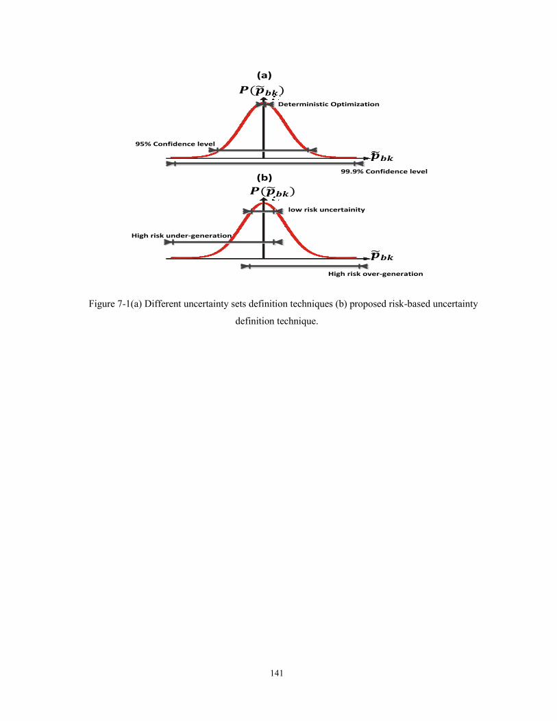
141
𝒑 𝒃𝒌
𝒑 𝒃𝒌
𝑷(𝒑 𝒃𝒌)
Deterministic Optimization
95% Confidence level
99.9% Confidence level
High risk over-generation
High risk under-generation
low risk uncertainity
(a)
(b)
𝑷(𝒑 𝒃𝒌)
Figure 7-1(a) Different uncertainty sets definition techniques (b) proposed risk-based uncertainty
definition technique.
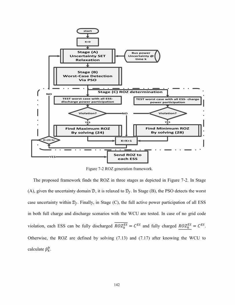
142
start
K=0
Stage (A)Uncertainty SET
Relaxation
Stage (B)Worst-Case Detection
Via PSO
Bus powerUncertainty @
time k
K=K+1K=24 hr
Send ROZ to each ESS
Violation?
TEST worst case with all ESS- discharge power participation
Violation?
TEST worst case with all ESS- charge power participation
Find Maximum ROZBy solving (24)
Find Minimum ROZBy solving (28)
YESYES
ON
YES
NOStage (C) ROZ determination
Figure 7-2 ROZ generation framework.
The proposed framework finds the ROZ in three stages as depicted in Figure 7-2. In Stage
(A), given the uncertainty domain 𝒟, it is relaxed to 𝒟𝑓. In Stage (B), the PSO detects the worst
case uncertainty within 𝒟𝑓. Finally, in Stage (C), the full active power participation of all ESS
in both full charge and discharge scenarios with the WCU are tested. In case of no grid code
violation, each ESS can be fully discharged 𝑅𝑂𝑍𝑘𝐸𝑆 = 𝐶𝐸𝑆 and fully charged 𝑅𝑂𝑍𝑘
𝐸𝑆 = 𝐶𝐸𝑆.
Otherwise, the ROZ are defined by solving (7.13) and (7.17) after knowing the WCU to
calculate 𝑝𝑘𝑏.

143
7.3.1 Stage A: Uncertainty Set Relaxation
In this stage, the uncertainty budget is calculated. It is considered as a weight for the
uncertainty set for reducing the conservatism of results due to extreme case uncertainty. An
uncertainty budget here is evaluated according to the uncertainty associated risk. In other words,
the less risky the uncertainty is, the more relaxed the uncertainty domain is. Further, the risk
probability is another factor in this process. This technique emulates the popular risk
management strategies that depend on two main factors to make decisions: the risk level and
the risk probability. The risk of the uncertainty focuses on its effect on voltage level, and a risk-
based-budget value is assigned, accordingly. For instance, if we study a bus voltage variation
for a wind turbine (with ∓20% power variation), normally it is windy with light load during
late night. As a result, extra wind generation is riskier on the bus voltage. Thus a high budget is
assigned for the UUL and lower for the ULL, and vice versa during peak hours (under-voltage
hours). On the other hand, for load uncertainty, the uncertainty budget maximizes the ULL
during overvoltage times, and vice versa during peak load hours (under-voltage). To quantify
the risk of uncertainty on the voltage level, the power with voltage relation is driven from the
famous voltage sensitivity matrix (the power flow inverse Jacobian). Assuming unity power
factor RES and constant power factor load, relation (7.21) is driven.
𝜕𝑣𝑘𝑏 = Λ𝑏𝑝𝜕𝑝𝑘
𝑏 + Λ𝑏𝑞𝜕𝑞𝑘𝑏 ∀ 𝑏𝜖𝒩𝑏 , ∀ 𝑘𝜖𝒩𝑘
𝜕𝑣𝑘𝑏 = 𝜕𝑝𝑘
𝑏(Λ𝑏𝑝 + Λ𝑏𝑞𝜆𝑙)
(7.21)
For studying the active power uncertainty at a bus b and a time k, critical power uncertainty
(CPU) limits [𝜕𝑝𝑘𝑏 , 𝜕𝑝𝑘
𝑏] are calculated in (7.22). It is worth noting that CPU is a function in
both the bus voltage in the deterministic case 𝑣𝑏𝑘(0) = arg (∅𝑘(𝒟 = 0)) and bus voltage

144
sensitivity. The upper CPU 𝜕𝑝𝑘𝑏 leads to a maximum overvoltage at the bus b, while the lower
CPU 𝜕𝑝𝑘𝑏 leads to under voltage limits in load buses sets and vice versa for lower CPU.
𝜕𝑝𝑘𝑏 =
𝑣 − 𝑣𝑘𝑏(0)
Λ𝑏𝑝 + Λ𝑏𝑞𝜆𝑙𝜕𝑝𝑘
𝑏 =𝑣 − 𝑣𝑘
𝑏(0)
Λ𝑏𝑝 + Λ𝑏𝑞𝜆𝑙
(7.22)
The uncertainty risk is calculated by comparing CPU and the uncertainty set limits. Further,
if different uncertainties PDFs are available, the risk probability is reachable. Calculating the
uncertainty budget from the uncertainty risk and the risk probability is not a straightforward
process; however, it is a logic process that can be efficiently solved by using logic rules.
Therefore, a fuzzy expert is proposed to tune the uncertainty budget limits using the risk and its
probability. The proposed fuzzy inference system has four inputs;
First; the UUL risk 𝑅𝑈𝑈𝐿𝑘𝑏 . It is the difference between the UUL and the maximum CPU. If
the uncertainty is higher than the critical power, the risk has a higher positive value which
means a higher risk, and vice versa.
𝑅𝑈𝑈𝐿𝑘𝑏 = 𝑝𝑘
𝑏 − 𝜕𝑝𝑘𝑏
(7.23)
The second input is ULL-risk 𝑅𝑈𝐿𝐿𝑘𝑏 . It is the difference between ULL and minimum CPU.
Both inputs are represented in per-unit.
𝑅𝑈𝐿𝐿𝑘𝑏
=𝑝𝑘𝑏−𝜕𝑝𝑘
𝑏 (7.24)
Finally, the third and fourth inputs are the risk probabilities’ values. As both 𝜕𝑝𝑘𝑏 , 𝜕𝑝𝑘
𝑏 are
deterministic, the risk probabilities are calculated from their CDF as follows; 𝜓(𝑅𝑈𝑈𝐿𝑏𝑘) =
𝜓 (𝑝𝑘𝑏) and 𝜓(𝑅𝑈𝑈𝐿𝑘
𝑏 ) = 𝜓(𝑝𝑘𝑏). If an uncertainty CDF is available for the uncertainties, then the
risk probabilities exist; otherwise, these probabilities are assumed as one (which means they
are unconsidered) and in such a case, the rule size shrinks from nine to three. That means that

145
the expert can still work without an exact CDF data. Each input is represented in the domain
of discourse by three membership functions [136], while the outputs are the uncertainty budget
limits Γ𝑘𝑏 , Γ𝑘
𝑏 which have five Gaussian membership functions, each within [0,1]. The expert
system has 18 rules given in Table 1 (first three rows are for the upper limit Γ𝑘𝑏, whereas the
last three rows are for the lower limit Γ𝑘𝑏).
Table 7-1 Fuzzy expert rules.
𝑅𝑈𝑈𝐿𝑘𝑏
𝜓(𝑅𝑈𝑈𝐿𝑘𝑏
)
positive zero Negative
Low probability V-Low Low Medium
Medium probability Low Medium High
High probability Medium High V-High
𝑅𝑈𝐿𝐿𝑘𝑏
𝜓(𝑅𝑈𝐿𝐿𝑘𝑏
)
negative zero Positive
Low probability V-Low Low Medium
Medium probability Low Medium High
High probability Medium High V-High
An easy way to define uncertain variable 𝜉 (given its uncertainty range [𝜉, 𝜉] and its average 𝜉)
is by using a triangular membership function centered at 𝜉, which expands by two linear lines to
the points (𝜉, 𝜉): however, if the CDF is given, other non-uniform presentations are possible.
Further details for deriving a membership function for an uncertain variable is given in [137],
while fuzzy risk management applications in power system restoration is discussed in [138].The
expert outputs are the weights of uncertainty budgets, which relax the original uncertainty set 𝒟
to get a filtered or un-conservative new set 𝒟𝑓.
𝒟𝑓 = {��𝑘𝑏𝜖ℝ𝑛𝑏 ×𝑛𝑘|��𝑘
𝑏𝜖 [Γ𝑘𝑏 𝑝𝑘
𝑏 , Γ𝑘𝑏 𝑝𝑘
𝑏] ∀ 𝑏𝜖𝒩𝑏 , ∀ 𝑘𝜖𝒩𝑘}
(7.25)

146
It is worth mentioning that the derived surface from Table 7-1 is a non-unique and sub-optimal
solution; however, it is derived using logic rules and empirical trials. As a future work, a
learning algorithm will be investigated to train the membership function parameters. It should
be noticed that other criterion rather than voltage level may be adopted to study the uncertainty
risk, such as voltage stability as adopted in [139], however, it is assumed that RES penetration
is not so high such that it threatens the voltage stability.
7.3.2 Stage B: Worst-Case Uncertainty Detection
Stage-B aims at defining the WCU over the relaxed uncertainty set 𝒟𝑓 using PSO. Not only
does PSO have a long history with power system applications, but also it has the following
advantages [140]. First, the fitness function is the gauge of the solution quality without the need
for complex calculations, such as gradient or matrix inversion calculations that may be
infeasible. This reduces the computational complexity and relaxes the continuity and convexity
conditions needed in gradient-based methods. Second, PSO is easily merged with other
optimization techniques (such as semi-definite programming in this chapter). Further, it can
escape local minima, as the scattered population results guide the solution. Finally, PSO is
preferred over other evolutionary algorithms for its simplicity, low memory requirement, and
fewer parameters tuning. On the other hand, like other heuristic algorithms, the solution may
have long calculation times depending on the population size and the initial position; however,
with the current developments in high-performance computing tools, less computational time is
achievable. Due to the aforementioned reasons, PSO is adopted as a WCU detector (𝑑∗) at
uncertainty domain 𝒟𝑓 hyper-plane. Each particle of the swarm-population 𝑋𝑘𝑗(𝜏) is a vector
with dimension 1×𝑛𝑏 represents the power uncertainties combination j calculated at future

147
sample time k at the PSO iteration 𝜏. The total population size equals 𝐽×𝐾. 𝒟𝑓 represents the
population search domain or the particles limits:
𝑋𝑘𝑗(𝜏) = ��𝑘
𝑏 = [��1𝑘𝑏𝑗(𝜏),… , ��𝑘𝑛𝑏
𝑏𝑗 (𝜏)] , 𝑋𝑘𝑗(𝜏)𝜖 𝒟𝑓
(7.26)
To detect the worst power uncertainty, the PSO maximizes a fitness function that represents
the sum of voltage deviation at all buses (penalty function 𝑓𝑉𝑘) in (7.27).
max (𝑓𝑉𝑘)∀𝑘
𝑓𝑉𝑘 = ∑1
1 + 𝑒−𝛼(𝑣−𝑣𝑘𝑏 )+
1
1 + 𝑒𝛼(��−𝑣𝑘𝑏 )+ 𝛽(𝑣𝑘
𝑏 − 𝑣𝑟)2
𝑛𝑏
𝑏=1
(7.27)
(7.28)
The penalty function consists of three parts: two sigmoid functions represent a very high
penalty for violating the desired voltage range and, the third part is a quadratic function that
penalizes the voltage deviation from the nominal 1.0 pu. Two remarks need to be highlighted
here. First, the choice of voltage deviation penalty function is not unique; however, the selection
of the function in such a shape assigns the voltage deviation a low penalty within the
permissible voltage zone but a much higher penalty for working outside this zone. Second, other
penalty functions are added easily, such as the branch ampacity limits (represented by the sum
of sigmoid functions centered at each branch maximum current or the power loss.
At a certain iteration 𝜏, after the penalty function is calculated for all J-particles, the local and
global best positions are updated and the new velocity vector is calculated for each particle as in
(7.29) . For solution quality, PSO must fulfill two important criteria: first, a high exploration at
the start of the search, and second, a deep exploitation to avoid trapping in a local-suboptimal
later [140]. Thus, a high speed for particles exploration is gained via high initial inertia that
reduces monotonically with the iterations progress to achieve higher exploitation later as in

148
(7.30). Next, the particles positions are updated as in (7.31). The reader is referred to [141] for
further details about PSO.
𝜔𝑘(𝜏) = 𝜔𝑚𝑎𝑥 −𝜔𝑚𝑎𝑥 − 𝜔𝑚𝑖𝑛
𝑀𝑎𝑥. 𝐼𝑡𝑒𝑟𝜏 (7.29)
𝑉𝑘𝑗(𝜏 + 1) = 𝜔𝑘(𝜏)𝑉𝑘
𝑗(𝜏) + 𝑐1𝑟1(𝑃𝑏𝑒𝑠𝑡𝑘
𝜏 − 𝑋𝑘𝑗(𝜏)) + 𝑐2𝑟2(𝐺𝑏𝑒𝑠𝑡𝑘
𝜏 − 𝑋𝑘𝑗(𝜏)) (7.30)
𝑋𝑘𝑗(𝜏 + 1) = 𝑉𝑘
𝑗(𝜏 + 1) + 𝑋𝑘
𝑗(𝜏) (7.31)
Finally, the stopping criterion is achieved in two cases; first, the convergence case happens if
the fitness function settles at a certain value within the predefined tolerance zone. This must
happen for a predefined number of iterations to guarantee convergence and avoid trapping in a
local minimum. Second, in an emergency case, it happens if the number of iterations exceeds
the maximum number (𝜏 ≥ 𝜏). After a stopping criterion is reached, the WCU is defined as the
global best position as 𝑊𝐶𝑈𝑘 = 𝐺𝑏𝑒𝑠𝑡𝑘.
Figure 7-3 depicts an example of a two -bus system with uncertain powers 𝑝1𝑘, 𝑝2𝑘 the
probabilistic distribution of the uncertainty is presented by two different Gaussian distributions.
The uncertainty domain 𝒟 is explained in the uncertainty space as follows 𝒟 =
{(𝑝1𝑘, 𝑝2𝑘)𝜖ℛ2×1|𝑝𝑏𝑘𝜖 [ 𝑝𝑏𝑘, 𝑝𝑏𝑘] ∀ 𝑏𝜖{1,2}}
. After applying stage A to define the uncertainty
risk via fuzzy expert, the domain is relaxed to 𝒟𝑓 =
{(𝑝1𝑘, 𝑝2𝑘)𝜖ℛ2×1|𝑝𝑏𝑘𝜖 [ Γb𝑝𝑏𝑘, Γb𝑝𝑏𝑘] ∀ 𝑏𝜖[1,2]}. Stage (B) detects the worst case uncertainty
(WCU) and found it at one of the vertices as depicted in Figure 7-3. This point is less
conservative than the original WCU.
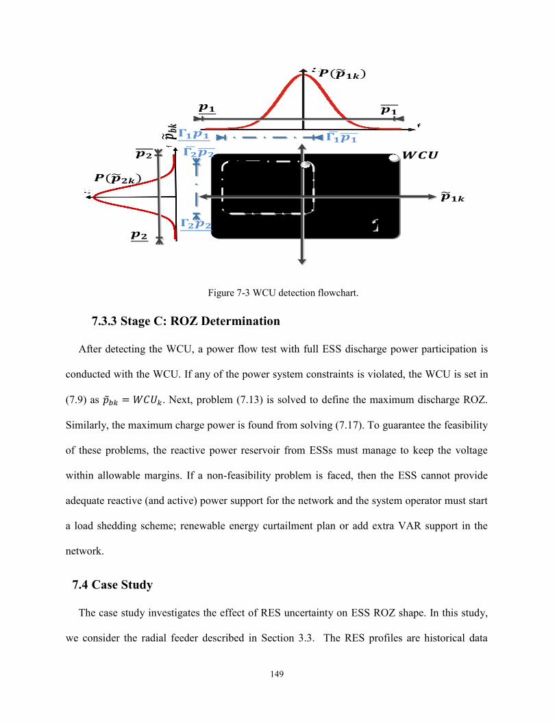
149
𝑷(𝒑 𝟏𝒌)
𝒑 𝒃𝒌
𝒑 𝟏𝒌
𝒑𝟏 𝒑𝟏
��𝒑𝟏 𝟏𝒑𝟏
��𝒑𝟐
𝟐𝒑𝟐
𝒑𝟐
𝒑𝟐
𝑷(𝒑 𝟐𝒌)
𝑾𝑪𝑼 𝒓𝒆𝒍𝒂𝒙𝒆𝒅 𝑾𝑪𝑼
Figure 7-3 WCU detection flowchart.
7.3.3 Stage C: ROZ Determination
After detecting the WCU, a power flow test with full ESS discharge power participation is
conducted with the WCU. If any of the power system constraints is violated, the WCU is set in
(7.9) as 𝑝𝑏𝑘 = 𝑊𝐶𝑈𝑘. Next, problem (7.13) is solved to define the maximum discharge ROZ.
Similarly, the maximum charge power is found from solving (7.17). To guarantee the feasibility
of these problems, the reactive power reservoir from ESSs must manage to keep the voltage
within allowable margins. If a non-feasibility problem is faced, then the ESS cannot provide
adequate reactive (and active) power support for the network and the system operator must start
a load shedding scheme; renewable energy curtailment plan or add extra VAR support in the
network.
7.4 Case Study
The case study investigates the effect of RES uncertainty on ESS ROZ shape. In this study,
we consider the radial feeder described in Section 3.3. The RES profiles are historical data
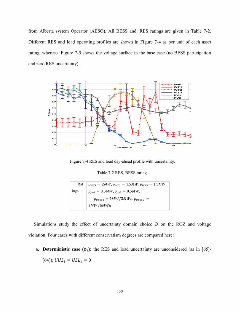
150
from Alberta system Operator (AESO). All BESS and, RES ratings are given in Table 7-2.
Different RES and load operating profiles are shown in Figure 7-4 as per unit of each asset
rating, whereas Figure 7-5 shows the voltage surface in the base case (no BESS participation
and zero RES uncertainty).
Figure 7-4 RES and load day-ahead profile with uncertainty.
Table 7-2 RES, BESS rating.
Rat
ings
𝑝𝑊𝑇1 = 2𝑀𝑊, 𝑝𝑊𝑇2 = 1.5𝑀𝑊, 𝑝𝑊𝑇3 = 1.5𝑀𝑊,
𝑝𝑝𝑣1 = 0.5𝑀𝑊, 𝑝𝑝𝑣2 = 0.5𝑀𝑊,
𝑝𝐵𝐸𝑆𝑆1 = 1𝑀𝑊/3𝑀𝑊ℎ, 𝑝𝐵𝐸𝑆𝑆2 =
2𝑀𝑊/6𝑀𝑊ℎ
Simulations study the effect of uncertainty domain choice 𝒟 on the ROZ and voltage
violation. Four cases with different conservatism degrees are compared here:
a. Deterministic case (𝓓𝟏): the RES and load uncertainty are unconsidered (as in [65]-
[64]); 𝑈𝑈𝐿1 = 𝑈𝐿𝐿1 = 0
0 5 10 15 200
0.1
0.2
0.3
0.4
0.5
0.6
0.7
0.8
0.9
1
Time (Hours)
PU P
ower
load
WT1
WT2
WT3
PV1
PV2
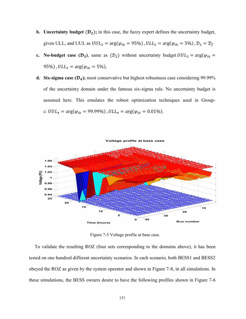
151
b. Uncertainty budget (𝓓𝟐); in this case, the fuzzy expert defines the uncertainty budget,
given ULL, and UUL as 𝑈𝑈𝐿2 = arg(𝜑𝑖𝑘 = 95%) , 𝑈𝐿𝐿2 = arg(𝜑𝑖𝑘 = 5%) ,𝒟2 = 𝒟𝑓
c. No-budget case (𝓓𝟑), same as (𝒟2) without uncertainty budget 𝑈𝑈𝐿3 = arg(𝜑𝑖𝑘 =
95%) , 𝑈𝐿𝐿3 = arg(𝜑𝑖𝑘 = 5%),
d. Six-sigma case (𝓓𝟒); most conservative but highest robustness case considering 99.99%
of the uncertainty domain under the famous six-sigma rule. No uncertainty budget is
assumed here. This emulates the robust optimization techniques used in Group-
c: 𝑈𝑈𝐿4 = arg(𝜑𝑖𝑘 = 99.99%) , 𝑈𝐿𝐿4 = arg(𝜑𝑖𝑘 = 0.01%).
Figure 7-5 Voltage profile at base case.
To validate the resulting ROZ (four sets corresponding to the domains above), it has been
tested on one hundred different uncertainty scenarios. In each scenario, both BESS1 and BESS2
obeyed the ROZ as given by the system operator and shown in Figure 7-8, in all simulations. In
these simulations, the BESS owners desire to have the following profiles shown in Figure 7-6
0
5
10
15
20
25
10
20
30
40
0.94
0.96
0.98
1
1.02
1.04
1.06
Bus number
Voltage profile at base case
Time (hours)
Volta
ge (P
U)
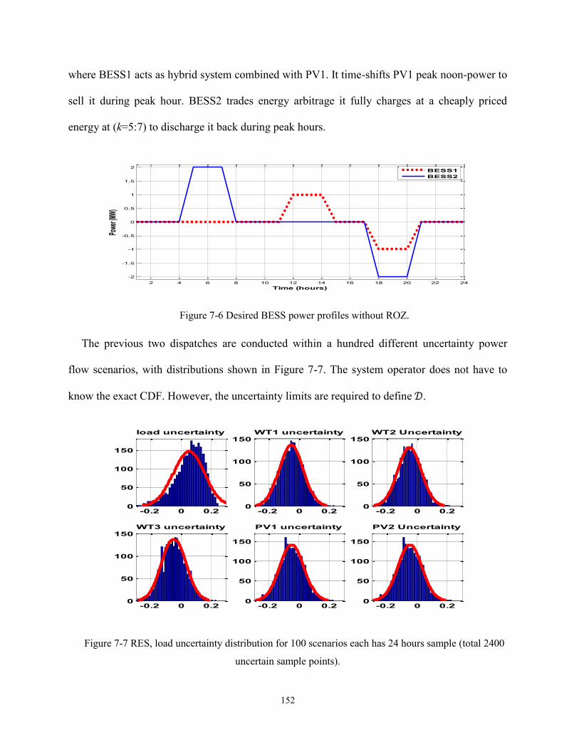
152
where BESS1 acts as hybrid system combined with PV1. It time-shifts PV1 peak noon-power to
sell it during peak hour. BESS2 trades energy arbitrage it fully charges at a cheaply priced
energy at (k=5:7) to discharge it back during peak hours.
Figure 7-6 Desired BESS power profiles without ROZ.
The previous two dispatches are conducted within a hundred different uncertainty power
flow scenarios, with distributions shown in Figure 7-7. The system operator does not have to
know the exact CDF. However, the uncertainty limits are required to define 𝒟.
Figure 7-7 RES, load uncertainty distribution for 100 scenarios each has 24 hours sample (total 2400
uncertain sample points).
2 4 6 8 10 12 14 16 18 20 22 24
-2
-1.5
-1
-0.5
0
0.5
1
1.5
2
Time (hours)
Powe
r (MW
)
BESS1
BESS2
-0.2 0 0.20
50
100
150
load uncertainty
-0.2 0 0.20
50
100
150WT1 uncertainty
-0.2 0 0.20
50
100
150WT2 Uncertainty
-0.2 0 0.20
50
100
150WT3 uncertainty
-0.2 0 0.20
50
100
150
PV1 uncertainty
-0.2 0 0.20
50
100
150
PV2 Uncertainty

153
Given 𝒟𝑖, 𝑖 = 1: 4, we calculate ROZ from (24) and (28) for each case of the different four
strategies. These ROZ are compared Figure 7-8. ROZ at each case is send to the ESSs to upper
limit the desired dispatch power depicted in Figure 7-6.
A comparison is conducted between the four cases by testing the hundred different
uncertainty scenarios generated from Figure 7-7. Further, the comparison is repeated at various
RES penetration levels (20, 30 and 40%). No contingency is assumed in all simulations. The
results are investigated from two perspectives. First, the network sound operation represented
here by buses’ voltage violations. This is represented here by the count of [over-voltage (OV) or
under-voltage (UV)] during the 100 scenarios. No ampacity violation occurs; thus they are not
included in the comparison. On the other hand, The ESS-owner cares about the ROZ size, as a
higher ROZ-size means a higher operation margin and profit. The ROZ-size is calculated
𝑅𝑂𝑍𝑆𝑠 =∫ (𝑝𝑠𝑘−𝑝𝑠𝑘)𝑑𝑘𝑛𝑘𝑘=0
∫ 2𝑆𝑠𝑑𝑘𝑛𝑘𝑘=0
∀𝑠 ∈ 𝒩𝑠.
A comparison between the gross violations (OV, UV) over the 100 different scenarios is
shown in Table 7-3. It compares the four ROZ cases corresponding to the various uncertainties.
Table 7-3. ROZ size and voltage violations in 100 scenarios.
20%-RES 30%-RES 40%-RES
OV U
V
ROZ2 OV UV ROZ2 O
V
U
V
ROZ2
𝒟1 133 47 98.2% 88 45 98% 43 41 97.6%
𝒟2 7 3 95.7% 7 1 95.7% 6 1 95.3%
𝒟3 6 2 95% 6 0 95.3% 5 1 94.9%
𝒟4 0 0 92.9% 0 0 92.9% 0 0 92.1%
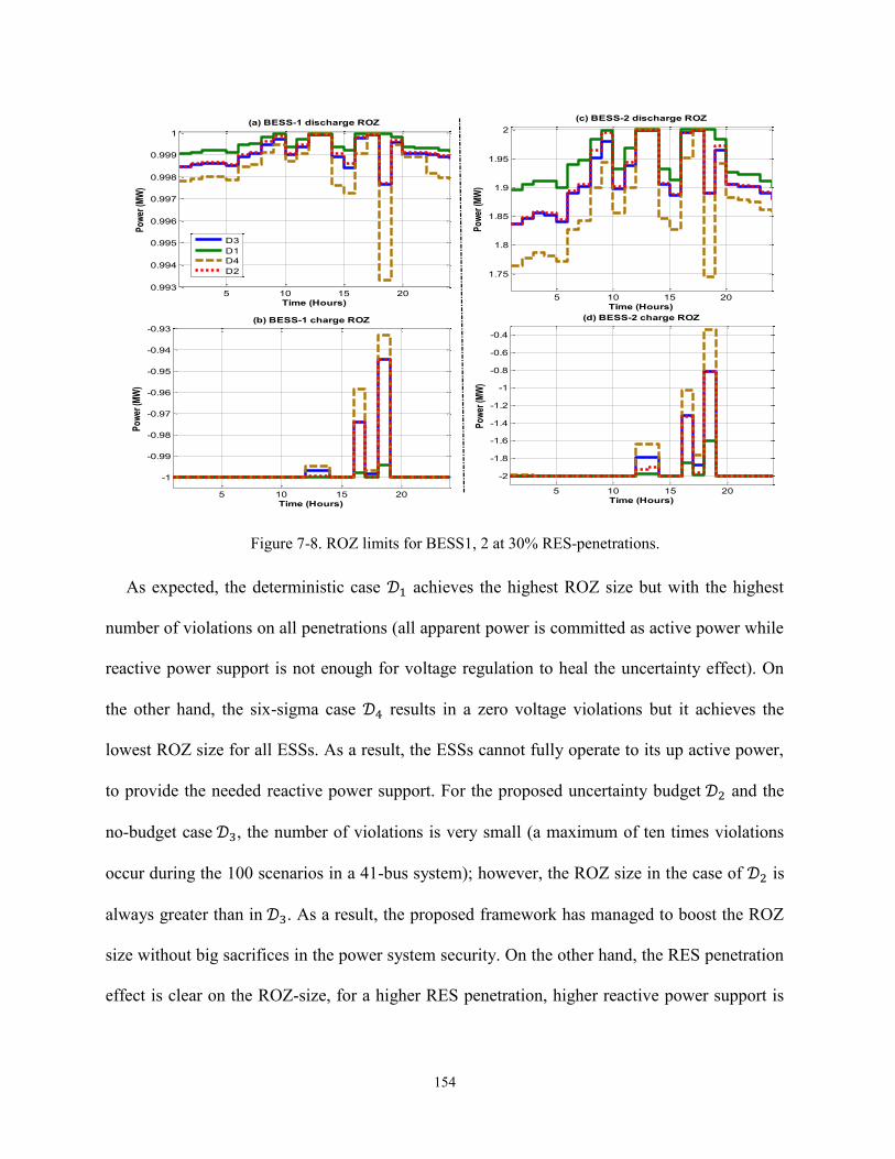
154
Figure 7-8. ROZ limits for BESS1, 2 at 30% RES-penetrations.
As expected, the deterministic case 𝒟1 achieves the highest ROZ size but with the highest
number of violations on all penetrations (all apparent power is committed as active power while
reactive power support is not enough for voltage regulation to heal the uncertainty effect). On
the other hand, the six-sigma case 𝒟4 results in a zero voltage violations but it achieves the
lowest ROZ size for all ESSs. As a result, the ESSs cannot fully operate to its up active power,
to provide the needed reactive power support. For the proposed uncertainty budget 𝒟2 and the
no-budget case 𝒟3, the number of violations is very small (a maximum of ten times violations
occur during the 100 scenarios in a 41-bus system); however, the ROZ size in the case of 𝒟2 is
always greater than in 𝒟3. As a result, the proposed framework has managed to boost the ROZ
size without big sacrifices in the power system security. On the other hand, the RES penetration
effect is clear on the ROZ-size, for a higher RES penetration, higher reactive power support is
5 10 15 200.993
0.994
0.995
0.996
0.997
0.998
0.999
1
Time (Hours)
Pow
er (M
W)
(a) BESS-1 discharge ROZ
5 10 15 20
1.75
1.8
1.85
1.9
1.95
2
Time (Hours)
Pow
er (M
W)
(c) BESS-2 discharge ROZ
5 10 15 20
-1
-0.99
-0.98
-0.97
-0.96
-0.95
-0.94
-0.93
Time (Hours)
Pow
er (M
W)
(b) BESS-1 charge ROZ
5 10 15 20
-2
-1.8
-1.6
-1.4
-1.2
-1
-0.8
-0.6
-0.4
Time (Hours)
Pow
er (M
W)
(d) BESS-2 charge ROZ
D3
D1
D4
D2

155
required from the ESSs. As a result, the active power limits decreases (ROZ size diminishes
with RES penetration).
7.5 Conclusions
This chapter presented a framework to define the ROZ for the power converters interfacing
distributed energy storage units. The technical constraints included permissible voltage level
and branches ampacity. The main work contribution is considering the power uncertainty while
reducing the results conservatism. The ROZ was calculated in three stages. First, a fuzzy-based
technique relaxes the uncertainty domain. Second, a PSO-based detection algorithm was
designed to determine the worst case uncertainty. Finally, a convex power flow problem defined
the ROZ. The proposed framework was tested on a real 41-bus radial feeder using different
uncertainty scenarios. Four uncertainty sets with different conservatism levels were compared.
The results showed that the proposed technique managed to boost the ESS participation with a
very low voltage and ampacity violations.

156
Chapter 8
8 Mobile Energy Storage Scheduling and Operation in Active
Distribution Systems
A mobile (transportable) energy storage system (MESS) can provide various services in
distribution systems including load leveling, peak shaving, reactive power support, renewable
energy integration and transmission deferral. Unlike stationary energy storage units, a mobile
energy storage system can move between different buses by truck to provide various local
services within the distribution feeder. This chapter proposes a day-ahead EMS for an MESS
that aims to minimize the cost of the power imported from the grid. The MESS does not only
shift renewable energy power to load peak hours but also can provide localized reactive power
support. Given day-ahead predictions for load and RES power, the EMS decides the optimal
MESS stations in the feeder and its operating power. Next, a particle swarm optimization-based
algorithm is developed to tune the moving time of the MESS according to a transit delay model.
The applicability of the proposed scheduling and operation algorithms is tested on a radial
distribution feeder.
8.1 Problem Description
8.1.1 Motivation
Still, with the increasing number of RESs dispersed in the system, a large number of ESSs is
needed to support the grid stability and reliability. This may result in an infeasible investment
from the economic point of view for two main reasons. First, the high cost of most of ESSs and

157
its relatively low lifetime. Second, the ESS cost diminishes with its rating; thus, a significant
number of ESSs is way much expensive than a single unit with the same ratings. According to
[105], the ESS power conversion system per-unit cost varies from (1,800$/kW) for a 5 kW
station compared to (300$/kW) for a 2 MW one as shown in Figure 8-1. As a result, a
significant saving is achievable if a single bulk ESS can replace a large number of smaller
ESSs. However, distributed ESSs provide some localized services that a single centralized ESS
cannot provide, such as voltage regulation or power loss minimization. An MESS solves this
problem because an MESS is a single ESS that can be plugged into the system at different
locations during different times, it can provide different localized grid services in a way much
cheaper than multi stationary ESSs (SESSs). The advantage of transportability is the ability to
deliver a localized reactive power support for voltage regulation, power loss reduction,
dispersed RESs integration, and last but not least, transmission and distribution upgrade
deferral.
Indeed, aggregated EVs look like a cheaper similar solution for providing grid services
exactly like the MESS. A similar solution where the network operator does not have to invest
any initial cost, however; aggregated EVs in parking lots have both power and energy
uncertainty due to their uncontrollable availability time [84] which question the reliability of the
service. Besides, it requires a high number of EVs to give the same power rating equivalent to a
single MESS truck. Finally, not all the EVs owners will be willing to participate in grid services
[83].
This study does not claim by any mean that an MESS will always prove to be financially
attractive than aggregated EVs or SESSs. Rather, a feasibility study that compares all the
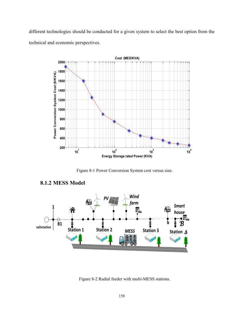
158
different technologies should be conducted for a given system to select the best option from the
technical and economic perspectives.
Figure 8-1 Power Conversion System cost versus size.
8.1.2 MESS Model
B1substation
1
b
Station 1 Station 2 Station Station 3MESS
Wind farm
PV
Smart house
𝓼 𝓑
Figure 8-2 Radial feeder with multi-MESS stations.
101
102
103
104
200
400
600
800
1000
1200
1400
1600
1800
2000
Energy Storage rated Power (KVA)
Po
we
r C
on
ve
rsio
n S
ys
tem
Co
st
($/K
VA
)Cost (MES/KVA)

159
Figure 8-2 shows an example of a radial feeder. The feeder has RESs set 𝒩𝑟 at different
locations of the feeder, such as wind energy conversion systems (WECS) and photovoltaic
(PV). Furthermore, other dispatchable resources (such as microturbines, small diesel engines,
etc.) may exist at different buses and defined by the set 𝒩𝑔. Moreover, the feeder has a load set
𝒩𝑙 with some smart houses (net-zero houses) that may use a rooftop PV, heat pumps, electric
storage, and electric vehicle. RESs have different profiles that can be forecasted efficiently
using both numerical and physical techniques (e.g., [65]). Moreover, electrical loads can be
accurately predicted for the day-ahead operation planning [142], [143]. It should be emphasized
that even with a 10-15% power prediction error, a day-ahead EMS cannot reach an optimal
solution; rather, day-ahead EMS provides a sub-optimal solution. To compensate for the
forecast error, a real-time controller is required to adjust the EMS solution depending on actual
system measurements. For instance, a day-ahead EMS decides the reactive power setpoint;
however, due to unpredictable real-time changes (sudden load change, faults or outages, RES
intermittency, etc.), the actual reactive power is tuned by a real-time on-line voltage controller
that measures the bus voltage and tunes the reactive power accordingly. This multi-level control
scheme has been adopted widely in the literature, such as in [28]. In power system dispatch, the
system operator adopts the same strategy when it comes to frequency control. The operator
measures the frequency deviation and the power imbalance to decide the area control error
(ACE), then the operator starts adjusting its day-ahead schedule by dispatching its reserve
resources in real-time accordingly to compensate the ACE [29].
The DNO can schedule an MESS to move between different positions for multi-services.
Different MESS positions (𝒩𝑠 ={1,2,..,𝓈}) define the buses at which the MESS can be
connected to the system which will be designated as the MESS-stations. Figure 8-3 depicts the
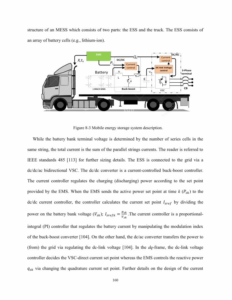
160
structure of an MESS which consists of two parts: the ESS and the truck. The ESS consists of
an array of battery cells (e.g., lithium-ion).
VSC
DC/DC
C
DC-link Voltagecontrol
Currentcontrol
EMS
Battery
CB
3-Phaseterminal
1 MW/3 MWh
Currentcontrol
Is Vdc
Qs
PsX,tx
L
DC/AC
Buck-boost
Figure 8-3 Mobile energy storage system description.
While the battery bank terminal voltage is determined by the number of series cells in the
same string, the total current is the sum of the parallel strings currents. The reader is referred to
IEEE standards 485 [113] for further sizing details. The ESS is connected to the grid via a
dc/dc/ac bidirectional VSC. The dc/dc converter is a current-controlled buck-boost controller.
The current controller regulates the charging (discharging) power according to the set point
provided by the EMS. When the EMS sends the active power set point at time k (𝑃𝑠𝑘) to the
dc/dc current controller, the controller calculates the current set point 𝐼𝑠𝑟𝑒𝑓 by dividing the
power on the battery bank voltage (𝑉𝑠𝑘); 𝐼𝑠𝑟𝑒𝑓𝑘 =𝑝𝑠𝑘
𝑉𝑠𝑘 .The current controller is a proportional-
integral (PI) controller that regulates the battery current by manipulating the modulation index
of the buck-boost converter [104]. On the other hand, the dc/ac converter transfers the power to
(from) the grid via regulating the dc-link voltage [104]. In the dq-frame, the dc-link voltage
controller decides the VSC-direct current set point whereas the EMS controls the reactive power
𝑞𝑠𝑘 via changing the quadrature current set point. Further details on the design of the current
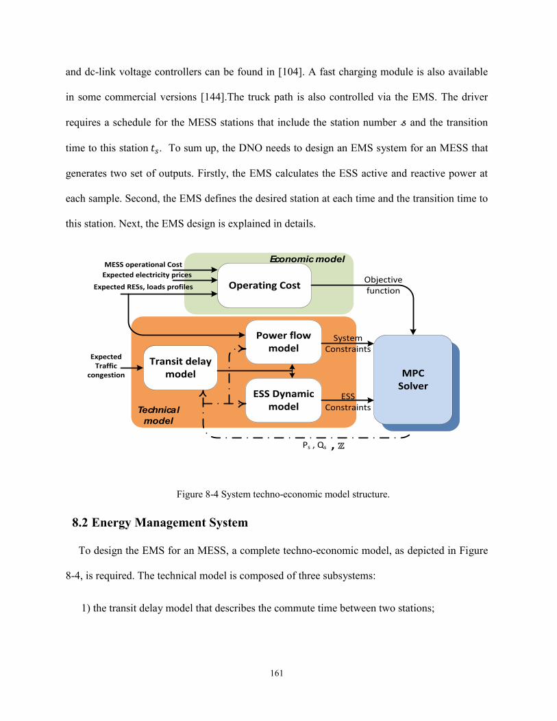
161
and dc-link voltage controllers can be found in [104]. A fast charging module is also available
in some commercial versions [144].The truck path is also controlled via the EMS. The driver
requires a schedule for the MESS stations that include the station number 𝓈 and the transition
time to this station 𝑡𝑠. To sum up, the DNO needs to design an EMS system for an MESS that
generates two set of outputs. Firstly, the EMS calculates the ESS active and reactive power at
each sample. Second, the EMS defines the desired station at each time and the transition time to
this station. Next, the EMS design is explained in details.
Transit delay model
ESS Dynamic model
Power flowmodel
Operating Cost
MPCSolver
Objectivefunction
Ps , Qs
SystemConstraints
ESSConstraints
MESS operational Cost
Expected electricity prices
Expected RESs, loads profiles
Expected Traffic
congestion
Economic model
Technical
model
, 𝕫
Figure 8-4 System techno-economic model structure.
8.2 Energy Management System
To design the EMS for an MESS, a complete techno-economic model, as depicted in Figure
8-4, is required. The technical model is composed of three subsystems:
1) the transit delay model that describes the commute time between two stations;

162
2) the power flow model that relates (the buses voltage, line current, and power loss) to the
MESS power and positions (e.g., as in Section 3.2.5);
3) the ESS dynamic model that represents the battery dynamics. The economic model
defines different costs of all resources that are reflected in the EMS objective function.
8.2.1 Transit Delay Model
The delay model depends on both time and stations positions. For a set of station𝑠 𝒩𝑠, the
distance between stations is defined by the distance matrix 𝐷𝑖𝑠𝑡 with a zero diagonal, any
element 𝑑𝑖𝑗∀𝑖, 𝑗 ∈ 𝒩𝑠 define the distance between stations (𝑖, 𝑗). In case 𝑑𝑖𝑗 = 𝑑𝑗𝑖, then the
MESS uses the same road between two stations (𝑖, 𝑗).
𝐷𝑖𝑠𝑡 = [0 ⋯ 𝑑1𝓈⋮ ⋱ ⋮𝑑𝓈1 ⋯ 0
] (8.1)
The traffic congestion delay 𝑡𝑐𝑖𝑗𝑘 is a time and location dependent index can give an
indicator [145] for the traffic delay. 𝜏𝑖𝑗𝑘is the commute time (in samples) from a station i to j at
time k ∈ 𝒩𝑘which is composed from three parts: the commute time, traffic congestion delay and
installation time
𝜏𝑖𝑗𝑘 = 𝑟𝑜𝑢𝑛𝑑(𝑡𝑐𝑖𝑗𝑘 + 𝑑𝑖𝑗𝑉𝑎𝑣𝑔 + 𝑡𝑖𝑛𝑠
𝑇𝑠 )∀𝑖, 𝑗 ∈ 𝒩𝑠, 𝑘 ∈ 𝒩𝑘, 𝑖 ≠ 𝑗
(8.2)
In (8.2), 𝑉𝑎𝑣𝑔 is the average truck speed, 𝑡𝑖𝑛𝑠 is the MESS installation time (the connection of
an MESS to the grid at the station). 𝑇𝑠 is the sample time in minutes. For the sake of the
modeling, let us define the Boolean matrix 𝕫 ∈ ℛ𝓈×𝒦, where each element 𝑧𝑖𝑘 equals one if the
MESS exists at station i at sample time k. Next, let us define the Boolean vector 𝕐 ∈ ℛ𝒦 that
represents the delay model. If the MESS is in transit at a sample T due to moving from a station
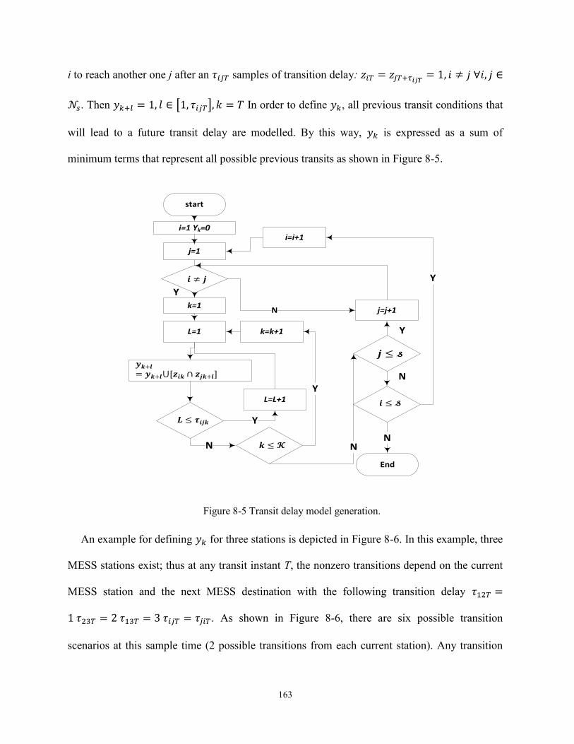
163
i to reach another one j after an 𝜏𝑖𝑗𝑇 samples of transition delay: 𝑧𝑖𝑇 = 𝑧𝑗𝑇+𝜏𝑖𝑗𝑇 = 1, 𝑖 ≠ 𝑗 ∀𝑖, 𝑗 ∈
𝒩𝑠. Then 𝑦𝑘+𝑙 = 1, 𝑙 ∈ [1, 𝜏𝑖𝑗𝑇], 𝑘 = 𝑇 In order to define 𝑦𝑘, all previous transit conditions that
will lead to a future transit delay are modelled. By this way, 𝑦𝑘 is expressed as a sum of
minimum terms that represent all possible previous transits as shown in Figure 8-5.
start
i=1 Yk=0
L=1
L=L+1
i=i+1
j=j+1
k=k+1
𝒊 ≤ 𝓼
𝒋 ≤ 𝓼
𝒌 ≤ 𝓚
𝑳 ≤ 𝝉𝒊𝒋𝒌
j=1
k=1
𝒊 ≠ 𝒋
𝒚𝒌+𝒍
= 𝒚𝒌+𝒍⋃[𝒛𝒊𝒌 ∩ 𝒛𝒋𝒌+𝒍]
Y
N
Y
N
Y
End
N
N
Y
Y
N
Figure 8-5 Transit delay model generation.
An example for defining 𝑦𝑘 for three stations is depicted in Figure 8-6. In this example, three
MESS stations exist; thus at any transit instant T, the nonzero transitions depend on the current
MESS station and the next MESS destination with the following transition delay 𝜏12𝑇 =
1 𝜏23𝑇 = 2 𝜏13𝑇 = 3 𝜏𝑖𝑗𝑇 = 𝜏𝑗𝑖𝑇. As shown in Figure 8-6, there are six possible transition
scenarios at this sample time (2 possible transitions from each current station). Any transition
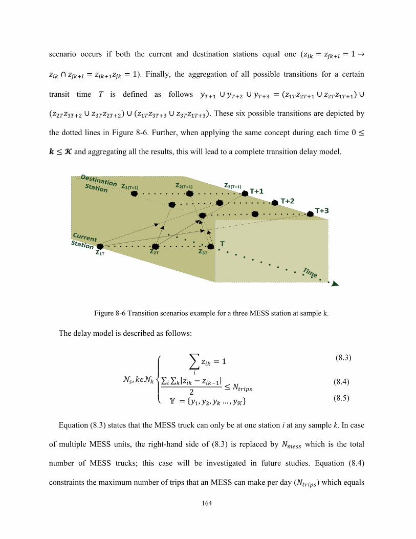
164
scenario occurs if both the current and destination stations equal one (𝑧𝑖𝑘 = 𝑧𝑗𝑘+𝑙 = 1 →
𝑧𝑖𝑘 ∩ 𝑧𝑗𝑘+𝑙 = 𝑧𝑖𝑘+1𝑧𝑗𝑘 = 1). Finally, the aggregation of all possible transitions for a certain
transit time T is defined as follows 𝑦𝑇+1 ∪ 𝑦𝑇+2 ∪ 𝑦𝑇+3 = (𝑧1𝑇𝑧2𝑇+1 ∪ 𝑧2𝑇𝑧1𝑇+1) ∪
(𝑧2𝑇𝑧3𝑇+2 ∪ 𝑧3𝑇𝑧2𝑇+2) ∪ (𝑧1𝑇𝑧3𝑇+3 ∪ 𝑧3𝑇𝑧1𝑇+3). These six possible transitions are depicted by
the dotted lines in Figure 8-6. Further, when applying the same concept during each time 0 ≤
𝒌 ≤ 𝓚 and aggregating all the results, this will lead to a complete transition delay model.
Z1(T+1)
Current Station
Destination Station
Time
T
T+1Z2(T+1) Z3(T+1)
Z1T Z2T Z3T
T+2T+3
Figure 8-6 Transition scenarios example for a three MESS station at sample k.
The delay model is described as follows:
𝒩𝑠, 𝑘𝜖𝒩𝑘
{
∑𝑧𝑖𝑘
𝑖
= 1
∑ ∑ |𝑧𝑖𝑘 − 𝑧𝑖𝑘−1|𝑘𝑖
2≤ 𝑁𝑡𝑟𝑖𝑝𝑠
𝕐 = {𝑦1, 𝑦2, 𝑦𝑘 … , 𝑦𝒦}
(8.3)
(8.4)
(8.5)
Equation (8.3) states that the MESS truck can only be at one station i at any sample k. In case
of multiple MESS units, the right-hand side of (8.3) is replaced by 𝑁𝑚𝑒𝑠𝑠 which is the total
number of MESS trucks; this case will be investigated in future studies. Equation (8.4)
constraints the maximum number of trips that an MESS can make per day (𝑁𝑡𝑟𝑖𝑝𝑠) which equals

165
half the number transitions. In case the MESS moved at time k from a station i to be at station j,
then 𝑧𝑖𝑘 = 0, 𝑧𝑖𝑘−1 = 1, 𝑧𝑗𝑘 = 1, 𝑧𝑗𝑘−1 = 0 and the sum of the difference at sample k is
calculated as ∑|𝑧𝑖𝑘−𝑧𝑖𝑘−1|
2= 1𝑖 , which means one trip is made. However, if the MESS stays at
station i at samples k and at k-1, then ∑|𝑧𝑖𝑘−𝑧𝑖𝑘−1|
2= 0𝑖 which means no trips are made. Finally,
(8.5) is a set of equalities that represent the transit flag 𝑦𝑘.
The power flow model is given by equations (3.34) to (3.48). It is worth mentioning that
other linearization techniques for the power flow are also possible as long as it provides a
convex constraint; otherwise, nonconvex optimization is needed to solve the EMS problem.
8.2.2 MESS Dynamic Model Considering the Transit Delay
The final part of the technical model is the ESS dynamics including the ESS power, total
number of cycles N, and the state of charge (SOC) which are expressed in (8.6)-(8.8).
In this model, we assume that anytime, there is always an ESS at each station s; however, the
constraint in (8.3) states that the MESS can be located at one unique station. Thus, the condition
for injecting discharge (𝑝𝑑ℎ𝑠𝑘) or importing charge power( 𝑝𝑐ℎ𝑠𝑘) at a certain bus s at time k is
that the MESS exists at this station (𝑧𝑠𝑘 = 1), and the MESS is not at transit state (𝑦𝑘 = 0).
These conditions are modelled by (8.6). Equation (8.7) expresses the SOC as an integrator. The
SOC equals one if the accumulated charge reaches the rated energy of the storage ��𝑠. The
charge and discharge efficiency is considered as 𝜂𝑐ℎ, 𝜂𝑑ℎ, respectively. As one MESS is
assumed at each bus, the total SOC is the sum of all stations ESS SOC at a certain time. A
similar technique is used for calculating the number of cycles 𝑁𝑘 that is assumed as an
integrator as well. The number of cycles is incremented by one each time a full charge is
absorbed by the MESS and injected again to the grid as expressed in (8.8).

166
{
𝑝𝑠𝑘 = (𝑝𝑐ℎ𝑠𝑘 + 𝑝𝑑ℎ𝑠𝑘)𝑧𝑠𝑘(1 − 𝑦𝑘)
𝑆𝑂𝐶𝑘+1 =∑𝑆𝑂𝐶𝑠𝑘 +𝑇𝑠
��𝑠 (𝜂𝑐ℎ𝑝𝑐ℎ𝑠𝑘 + 𝜂𝑑ℎ𝑝𝑑ℎ𝑠𝑘)𝑧𝑠𝑘(1 − 𝑦𝑘)
𝑠
𝑁𝑘+1 =∑𝑁𝑠𝑘 +𝑇𝑠(𝑝𝑐ℎ𝑠𝑘 − 𝑝𝑑ℎ𝑠𝑘)
2��𝑠𝑧𝑠𝑘(1 − 𝑦𝑘)
𝑠
∀𝑘𝜖𝒩𝑘, 𝑠𝜖𝒩𝑠, 𝜂𝑐ℎ < 1, 𝜂𝑑ℎ > 1
(8.6)
(8.7)
(8.8)
The dynamic ESS constraints are stated in (8.9)-(8.12). While constraints (8.9) and (8.10)
define the charge and discharge powers as positive and negative power limited by the thermal
limit of the MESS, constraint (8.11) limits the apparent power of the MESS to be upper
bounded by the rated MESS apparent power (𝑆) at any time. The discrete variable 𝑐𝑒𝑘
guarantees that charging and discharging are mutually exclusive. If 𝑐𝑒𝑘 equals one, the charging
limits are between rated power and zero while discharge power is zero. On the other hand,
setting𝑐𝑒𝑘 to zero allows discharging and limits charging power to zero. The SOC is limited in
(8.12) between the desired minimum SOC 𝑆𝑂𝐶 and one to avoid deep discharge and
overcharging that may reduce the battery life dramatically. Further, the number of cycles at the
end of the day is limited by (8.13) as the battery life is a countable number of cycles.
0 ≤ 𝑝𝑐ℎ𝑠𝑘 ≤ ��𝑠(𝑐𝑒𝑠)
− ��𝑠(1 − 𝑐𝑒𝑠) ≤ 𝑝𝑑ℎ𝑠𝑘 ≤ 0
𝑝𝑠𝑘2 + 𝑞𝑠𝑘
2 ≤ 𝑆
𝑆𝑂𝐶 ≤ 𝑆𝑂𝐶𝑘 ≤ 1
𝑁𝒦 ≤ 𝑁∀ 𝑏𝜖𝒩𝑏 , 𝑡𝜖𝒩𝑡 , 𝑘𝜖𝒩𝑘
(8.9)
(8.10)
(8.11)
(8.12)
(8.13)
8.2.3 Original EMS Problem
The EMS objective is maximizing the day-ahead profit for the DNO by minimizing the
imported energy cost from the grid (energy arbitrage). It is assumed that the MESS is an asset
owned by the DNO to provide both reactive power support and maximize net profit. RESs are
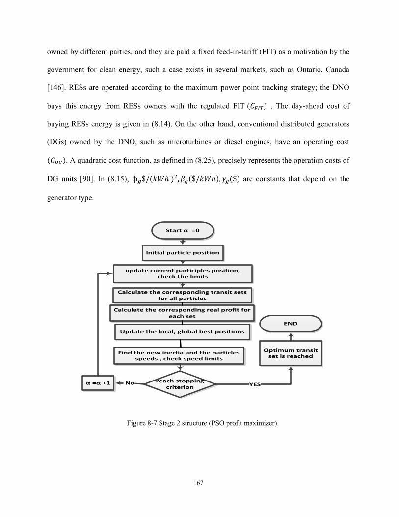
167
owned by different parties, and they are paid a fixed feed-in-tariff (FIT) as a motivation by the
government for clean energy, such a case exists in several markets, such as Ontario, Canada
[146]. RESs are operated according to the maximum power point tracking strategy; the DNO
buys this energy from RESs owners with the regulated FIT (𝐶𝐹𝐼𝑇) . The day-ahead cost of
buying RESs energy is given in (8.14). On the other hand, conventional distributed generators
(DGs) owned by the DNO, such as microturbines or diesel engines, have an operating cost
(𝐶𝐷𝐺). A quadratic cost function, as defined in (8.25), precisely represents the operation costs of
DG units [90]. In (8.15), ϕ𝑔$/(𝑘𝑊ℎ )2, 𝛽𝑔($/𝑘𝑊ℎ), 𝛾𝑔($) are constants that depend on the
generator type.
Start α =0
Initial particle position
update current participles position, check the limits
Calculate the corresponding transit sets for all particles
Update the local, global best positions
Find the new inertia and the particles speeds , check speed limits
α =α +1 reach stopping criterion
Optimum transit set is reached
END
No YES
Calculate the corresponding real profit for each set
Figure 8-7 Stage 2 structure (PSO profit maximizer).

168
𝐶𝐷𝐺 = ∑∑𝜙𝑔(𝑝𝑔𝑘𝑇𝑠)2+ 𝛽𝑔(𝑝𝑔𝑘𝑇𝑠) + 𝛾𝑔
ℊ
𝑔=1
𝒦
𝑘=1
𝐶𝑟𝑒𝑠 = ∑∑𝑝𝑟𝑘𝑇𝑠𝐶𝐹𝐼𝑇
ℜ
𝑟=1
𝒦
𝑘=1
(8.13)
(8.14)
The MESS cost 𝐶𝑚𝑒𝑠𝑠 includes both the truck operating cost 𝐶𝑡𝑟𝑢𝑐𝑘 and the ESS cost 𝐶𝑒𝑠𝑠 as
in (8.15). Firstly, the truck operating cost (8.16) includes a fuel cost and labor cost. While the
fuel cost is modelled as a worst case cost (the multiplication of maximum distance (in km) by
the number of the trips by the fuel consumption cost 𝐹𝐶 ($/𝑘𝑚)), the truck labor cost 𝑡𝑙𝑐
includes the daily stipend of the truck driver and technicians. Secondly, (8.17) models the ESS
cost as a levelized cost (𝐶𝑘𝑤ℎ$/𝑘𝑊ℎ 𝑐ℎ𝑎𝑟𝑔𝑒𝑑). This cost is adopted before for ESS in [38].
However, the capital cost is modified to include the truck capital cost and ESS maintenance cost
that includes the truck maintenance cost.
𝐶𝑚𝑒𝑠𝑠 = 𝐶𝑡𝑟𝑢𝑐𝑘 + 𝐶𝑒𝑠𝑠𝐶𝑡𝑟𝑢𝑐𝑘 = 𝐹𝐶×𝑁𝑡𝑟𝑖𝑝×max(𝐷𝑖𝑠𝑡) + 𝑡𝑙𝑐
𝐶𝑒𝑠𝑠 = ∑∑𝑃𝑐ℎ𝑠𝑘𝑇𝑠𝐶𝑘𝑤ℎ
𝓈
𝑠=1
𝒦
𝑘=1
(8.15)
(8.16)
(8.17)
The final cost item is the grid power cost 𝐶𝑔𝑟𝑖𝑑 that is the multiplication of the expected pool
price (buy price) 𝐵𝑃𝑘($/𝑘𝑊ℎ) and the grid energy 𝑃𝑔𝑟𝑖𝑑𝑘𝑇𝑠 as shown in (8.18). This cost has a
negative value (becomes income) in case the distribution system exports surplus energy to the
grid. The income of the DNO is generated from daily selling energy to the loads with the sell
price 𝑆𝑃𝑘($/𝑘𝑊ℎ) as given in (8.19). Finally, the profit is the difference between the income
and the costs (MESS operating cost, DG running cost plus RES energy purchasing cost) as
shown in (8.20).

169
𝐶𝑔𝑟𝑖𝑑 = ∑𝑇𝑠𝐵𝑃𝑘𝑃𝑔𝑟𝑖𝑑𝑘
𝒦
𝑘=1
, 𝑃𝑔𝑟𝑖𝑑𝑘 = 𝑃𝑏𝑘, 𝑏 = 0
𝑖𝑛𝑐 = ∑∑𝑇𝑠𝑆𝑃𝑘𝑃𝑙𝑘
ℒ
𝑙=1
𝒦
𝑘=1
𝑝𝑟𝑜 = 𝑖𝑛𝑐 − 𝐶𝑔𝑟𝑖𝑑 − 𝑐𝑚𝑒𝑠𝑠 − 𝐶𝐷𝐺 − 𝐶𝑟𝑒𝑠
(8.18)
(8.19)
(8.20)
The final optimization problem is expressed as follows
max𝑝𝑐ℎ𝑠𝑘,𝑝𝑑ℎ𝑠𝑘 ,ℤ,𝑞𝑠𝑘
(𝑝𝑟𝑜)
𝑆. 𝑡. (3.34) − (3.48)& (8.3) − (8.13),
(8.21)
The problem in (8.21) is a mixed integer nonconvex problem that may face a feasibility
problem and does not guarantee to reach a global optimal solution in a certain time. In Section
IV, this problem will be converted to a mixed integer convex problem using the proposed two-
stage EMS.
8.3 Two-Stage EMS
To convert the problem in (8.21) into a mixed integer convex problem, the following
suboptimal two-stage solution is proposed. Firstly, the problem is solved assuming
instantaneous MESS transit; this problem calculates the MESS designated stations and its transit
times (given the previous assumption). Secondly, a particle swarm algorithm optimizes the
transit periods of the first stage without changing the MESS stations.
8.3.1 Stage 1 (Instantaneous Transit EMS)
The delay model 𝕐 given in (8.5) is a nonlinear sophisticated Boolean expression that
depends on both the truck transit time and stations ℤ. Assuming that 𝕐 = 0 or MESS can move
instantaneously from a station to another will reduce the problem complexity on the price of
sub-optimality, this part will be discussed later. The MESS model is expressed as a linear set of
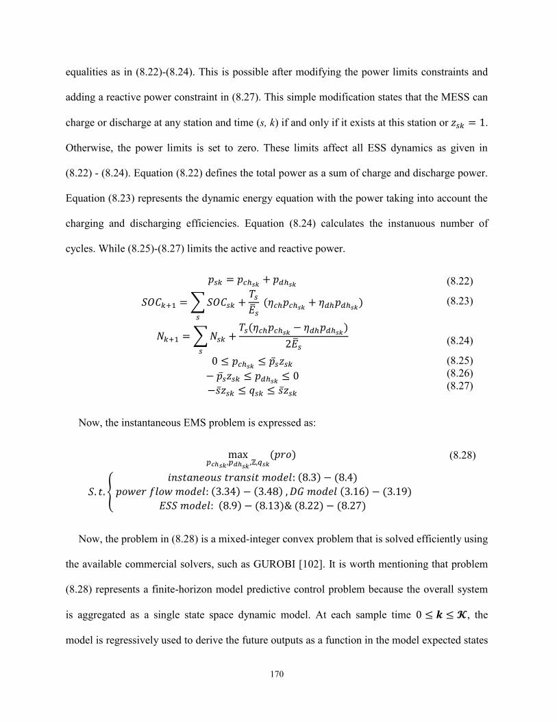
170
equalities as in (8.22)-(8.24). This is possible after modifying the power limits constraints and
adding a reactive power constraint in (8.27). This simple modification states that the MESS can
charge or discharge at any station and time (s, k) if and only if it exists at this station or 𝑧𝑠𝑘 = 1.
Otherwise, the power limits is set to zero. These limits affect all ESS dynamics as given in
(8.22) - (8.24). Equation (8.22) defines the total power as a sum of charge and discharge power.
Equation (8.23) represents the dynamic energy equation with the power taking into account the
charging and discharging efficiencies. Equation (8.24) calculates the instanuous number of
cycles. While (8.25)-(8.27) limits the active and reactive power.
𝑝𝑠𝑘 = 𝑝𝑐ℎ𝑠𝑘 + 𝑝𝑑ℎ𝑠𝑘
𝑆𝑂𝐶𝑘+1 =∑𝑆𝑂𝐶𝑠𝑘 +𝑇𝑠
��𝑠 (𝜂𝑐ℎ𝑝𝑐ℎ𝑠𝑘 + 𝜂𝑑ℎ𝑝𝑑ℎ𝑠𝑘)
𝑠
𝑁𝑘+1 =∑𝑁𝑠𝑘 +𝑇𝑠(𝜂𝑐ℎ𝑝𝑐ℎ𝑠𝑘 − 𝜂𝑑ℎ𝑝𝑑ℎ𝑠𝑘)
2��𝑠𝑠
0 ≤ 𝑝𝑐ℎ𝑠𝑘 ≤ ��𝑠𝑧𝑠𝑘− ��𝑠𝑧𝑠𝑘 ≤ 𝑝𝑑ℎ𝑠𝑘 ≤ 0
−��𝑧𝑠𝑘 ≤ 𝑞𝑠𝑘 ≤ ��𝑧𝑠𝑘
(8.22)
(8.23)
(8.24)
(8.25)
(8.26)
(8.27)
Now, the instantaneous EMS problem is expressed as:
max𝑝𝑐ℎ𝑠𝑘,𝑝𝑑ℎ𝑠𝑘 ,ℤ,𝑞𝑠𝑘
(𝑝𝑟𝑜)
𝑆. 𝑡. {
𝑖𝑛𝑠𝑡𝑎𝑛𝑒𝑜𝑢𝑠 𝑡𝑟𝑎𝑛𝑠𝑖𝑡 𝑚𝑜𝑑𝑒𝑙: (8.3) − (8.4)
𝑝𝑜𝑤𝑒𝑟 𝑓𝑙𝑜𝑤 𝑚𝑜𝑑𝑒𝑙: (3.34) − (3.48) , 𝐷𝐺 𝑚𝑜𝑑𝑒𝑙 (3.16) − (3.19)
𝐸𝑆𝑆 𝑚𝑜𝑑𝑒𝑙: (8.9) − (8.13)& (8.22) − (8.27)
(8.28)
Now, the problem in (8.28) is a mixed-integer convex problem that is solved efficiently using
the available commercial solvers, such as GUROBI [102]. It is worth mentioning that problem
(8.28) represents a finite-horizon model predictive control problem because the overall system
is aggregated as a single state space dynamic model. At each sample time 0 ≤ 𝒌 ≤ 𝓚, the
model is regressively used to derive the future outputs as a function in the model expected states

171
and the future control action along the prediction horizon [123]. The inputs of the state-space
model are the MESS power and locations [𝑧𝑖𝑘, 𝑝𝑠𝑘 , 𝑞𝑠𝑘], whereas the system states are the SOC
and number of cycles [𝑆𝑂𝐶𝑠𝑘, 𝑁𝑠𝑘]. Finally, the controlled outputs are any constrained variable
in the system, such as [𝑆𝑂𝐶𝑘, 𝑁𝑘, 𝑝𝑠𝑘, 𝑞𝑠𝑘, 𝓅𝑡𝑘 , … ] .
8.3.2 Stage 2 (PSO Profit Maximizer)
The resulting profit from Stage 1 is not the actual profit. In reality, the MESS transit period is
not zero, and every time the MESS moves from a station i at instant 𝜆 heading to another station
j, it will stay in transit for a period 𝜏𝑖𝑗𝑘 defined by (8.2) till it reaches its destination at instant
𝜆 + 𝜏𝑖𝑗𝜆. The set of time indices that define that the MESS is at transit state is 𝒩𝜏:
𝒩𝜏 = {[𝜆, 𝜆 + 𝜏𝑖𝑗𝜆]|𝑧𝑖𝜆 = 𝑧𝑗𝜆−1 = 1∀𝑖 ≠ 𝑗, 𝑖, 𝑗 ∈ (8.29)
Now, if the MESS is at transit, that means that the DNO has to buy (or sell) the MESS
scheduled energy from the grid till the MESS reaches its next destination. Further, the MESS is
not operating during transit periods, thus its operating cost 𝐶𝑒𝑠𝑠 should not be considered as
well. The real profit ℛ𝑝𝑟𝑜 when the transit set 𝒩𝜏 is taken into account is
ℛ𝑝𝑟𝑜 = 𝑝𝑟𝑜 + ∑ ∑ 𝑇𝑠𝐵𝑃𝜆𝑝𝑠𝜆𝑠∈𝒩𝑠
+ ∑ ∑ 𝑃𝑐ℎ𝑠𝜆𝑇𝑠𝐶𝑘𝑤ℎ𝑠∈𝒩𝑠𝜆𝜖𝒩𝜏𝜆𝜖𝒩𝜏
(8.30)
It is worth mentioning that if 𝑝𝑠𝜆 < 0, which means the MESS is discharging at this time;
however, as the MESS is in the transit state, this energy ∑ 𝑇𝑠𝑝𝑠𝜆𝑠∈𝒩𝑠is exported from the grid
with a price 𝐵𝑃𝜆 at this time. On the contrary, if the MESS is supposed to be charged at this
time, the surplus system energy is sold to the grid with this time price (or even worse, RESs
energy can be curtailed in case the voltage level or thermal current levels are violated). Further,
the ESS cost is excluded from the profit calculation during time periods flagged in 𝒩𝜏. Not

172
only, is the profit and power system is affected by the delay, but also the ESS dynamics as well.
For instance, the real SOC (ℛ𝑆𝑂𝐶) after considering the transit delay is defined as in (8.31).
The SOC is normally calculated in the non-transit case, while it stays fixed during transit as the
ESS is in the stand-by mode. Other ESS dynamics, such as the real number of cycles ℛ𝑁 is
calculated as in (8.32).
{ℛ𝑆𝑂𝐶𝑘+1 =∑ℛ𝑆𝑂𝐶𝑠𝑘 +
𝑇𝑠
��𝑠 (𝜂𝑐ℎ𝑝𝑐ℎ𝑠𝑘 + 𝜂𝑑ℎ𝑝𝑑ℎ𝑠𝑘)
𝑠
, 𝑘 ∈ 𝒩𝑘 −𝒩𝜏
ℛ𝑆𝑂𝐶𝑘+1 = ℛ𝑆𝑂𝐶𝑘, 𝑘 ∈ 𝒩𝜏
{ℛ𝑁𝑘+1 =∑ℛ𝑁𝑠𝑘 +
𝑇𝑠(𝜂𝑐ℎ𝑝𝑐ℎ𝑠𝑘 − 𝜂𝑑ℎ𝑝𝑑ℎ𝑠𝑘)
2��𝑠𝑠
, 𝑘 ∈ 𝒩𝑘 −𝒩𝜏
ℛ𝑁𝑘+1 = ℛ𝑁𝑘, 𝑘 ∈ 𝒩𝜏
(8.31)
(8.32)
One needs to make sure that the transit set will not lead to ESS dynamic constraint violation.
For instance, one transit set can move the MESS very early from discharge stations and very
late from charging station, thus an overcharge may occur and vice versa. One solution to this
problem is keeping a reserve in the capacity (e.g., the SOC limits are chosen from 20 to 90 %)
to account for possible uncertainties.
The PSO optimizer defines optimum transit delay set 𝒩𝜏 that maximizes the real profit
without violating the ESS dynamics. Firstly, each particle 𝑥𝑛 represents a different transit set
𝒩𝜏𝑛 by changing the transit time 𝜆𝛼
𝑛 , where n is the index for the particle in the population, and
𝛼 is the index for the transit time. Normally, the number of transits is less than or equal 𝑁𝑡𝑟𝑖𝑝𝑠
𝑥𝑛 = [𝜆1𝑛, 𝜆2
𝑛, . . , 𝜆𝑁𝑡𝑟𝑖𝑝𝑠
𝑛 ]
𝒩𝜏𝑛 = {[𝜆1
𝑛, 𝜆1𝑛 + 𝜏𝑖𝑗𝜆1𝑛], [𝜆2
𝑛, 𝜆2𝑛 + 𝜏𝑖𝑗𝜆2𝑛]. . [𝜆𝑁𝑡𝑟𝑖𝑝𝑠
𝑛 , 𝜆𝑁𝑡𝑟𝑖𝑝𝑠
𝑛 + 𝜏𝑖𝑗𝜆𝑁𝑡𝑟𝑖𝑝𝑠𝑛 ]
𝜆𝛼 −𝑀 ≤ 𝜆𝛼𝑛 ≤ 𝜆𝛼 +𝑀, 1 ≤ 𝛼 ≤ 𝑁𝑡𝑟𝑖𝑝𝑠
(8.33)
(8.34)
(8.35)

173
As shown, the particle 𝑥𝑛 is a randomly generated vector for the transit and is bounded by
that defines the maximum shift in the transit time within a band [−𝑀,𝑀]. The swarm
population 𝕏 is then defined with a population-size 𝓃 particles, each has a corresponding transit
set defined in (8.36).
𝕏 = {𝑥1, 𝑥2…𝑥𝑛 …𝑥𝓃}
ℕ = {𝒩𝜏1,𝒩𝜏
2…𝒩𝜏𝑛…𝒩𝜏
𝓃}
(8.36)
(8.37)
The real profit is calculated for each particle, and the local and global best particle positions
are allocated. At each iteration 𝛼, after the profit is calculated for all 𝕩 set-particles, the local
and global best positions 𝑃𝑏𝑒𝑠𝑡(𝛼), 𝐺𝑏𝑒𝑠𝑡(𝛼) are updated and the new velocity for the next
sample (𝑉𝑛(𝛼 + 1)) for each particle n is calculated as in (8.39). For solution quality, the PSO
algorithm must fulfill two important criteria: first, a high exploration at the start of the search,
and second, a deep exploitation to avoid trapping in a local-suboptimal later [140]. Thus, a high
speed for particles exploration is gained via high initial inertia that reduces monotonically with
the iterations progress in order to achieve higher exploitation later. This is possible by updating
the PSO inertia 𝜔(𝛼) as in (8.38) starting from the desired minimum value 𝜔𝑚𝑖𝑛 at the first
search sample and reaching its peak 𝜔𝑚𝑎𝑥 at the maximum iteration value 𝑀𝑎𝑥. 𝐼𝑡𝑒𝑟. Next, the
particles positions are updated as in (8.40). The reader is referred to [140] for further details on
the PSO algorithm. Finally, the stopping criterion is achieved in two cases. Firstly, the
convergence case happens if the fitness function (real profit) settles at a certain value within the
predefined tolerance zone.
𝜔(𝛼) = 𝜔𝑚𝑎𝑥 −𝜔𝑚𝑎𝑥 − 𝜔𝑚𝑖𝑛
𝑀𝑎𝑥. 𝐼𝑡𝑒𝑟𝛼
𝑉𝑛(𝛼 + 1) = 𝜔(𝛼)𝑉𝑛(𝛼) + 𝑐1𝑟1(𝑃𝑏𝑒𝑠𝑡 − 𝑥𝑛(𝛼)) + 𝑐2𝑟2(𝐺𝑏𝑒𝑠𝑡 − 𝑥𝑛(𝛼))
𝑥𝑛(𝛼 + 1) = 𝑉𝑛(𝛼 + 1) + 𝑥𝑛(𝛼)
(8.38)
(8.39)
(8.40)
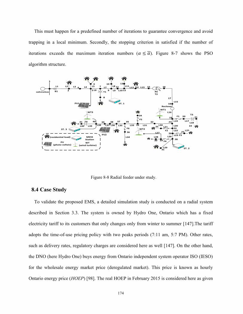
174
This must happen for a predefined number of iterations to guarantee convergence and avoid
trapping in a local minimum. Secondly, the stopping criterion in satisfied if the number of
iterations exceeds the maximum iteration numbers (𝛼 ≤ 𝛼). Figure 8-7 shows the PSO
algorithm structure.
B1 T1 RST2
Recloser
T3
T4
F1
F2
F3
F4
F5
F6
L2L1 L3 L4 L5
L6
L7L8
L9 L10
L11L12 L13
L15
L16
L17L18
L19
L20L21
L22
L23
L25
L26
L27
L28
L29
L30L31L33
L34
L35L36L37L38
substation
1
2
4
5
67
8
9
10
11
12
13
14 15 16
17
18
1920 21
22
2332
33
34
35
36
37383941
2425
2627
282930
31
40
PV1
PV2
WT1
WT2
ST. 2
(residential load) MESSStation
WT (wind turbine)
PV (photo voltaic)
ST. 1
ST. 3
L39L40
WT3
Figure 8-8 Radial feeder under study.
8.4 Case Study
To validate the proposed EMS, a detailed simulation study is conducted on a radial system
described in Section 3.3. The system is owned by Hydro One, Ontario which has a fixed
electricity tariff to its customers that only changes only from winter to summer [147].The tariff
adopts the time-of-use pricing policy with two peaks periods (7:11 am, 5:7 PM). Other rates,
such as delivery rates, regulatory charges are considered here as well [147]. On the other hand,
the DNO (here Hydro One) buys energy from Ontario independent system operator ISO (IESO)
for the wholesale energy market price (deregulated market). This price is known as hourly
Ontario energy price (HOEP) [98]. The real HOEP in February 2015 is considered here as given

175
in [98]. The HOEP and DNO tariff (buy and sell prices) are shown in Figure 8-9(c). RESs’
owners are paid a feed-in-tariff (𝑐𝐹𝐼𝑇) decided by IESO as given in [148], and it is presented in
table 8-1. No utility-owned DGs exist in the system under study; however, DGs can be easily
dispatched by considering their active and reactive power limits, and, power rate constraints as
detailed in [90].
The MESS optimal sizing is conducted in Chapter 4. The storage cost is 600 K$/MWh and
the conversion system cost is 350K$/MW [100], while the operation and maintenance cost for
MESS are assumed to be 12k$/year including the ESS and the truck, the truck cost is assumed
to be 50K$. After making stochastic sizing using these input data, an optimal size of the MESS
is found to be 3250 kVA/6381.3 kWh which equals 4.247 Million $. The MESS efficiency and
cost parameters are stated in Table 9-1. According to [29], lithium-ion batteries have an energy
density of 0.25 kWh/kg and the power density is 0.5 kW/kg. Applying that in our MESS case
results in a 32-ton load which is a suitable load for a tow truck with an acceptable cost [149].
The MESS is assumed to participate 250 cycles/year with results in a 3000 cycle per its
lifetime (here 12 years), Assuming more cycles makes the profit negative, and the whole
investment becomes void especially when a replacement cost will be considered. The distance
between different stations is given in Table 9-1. Finally, for the MESS delay model, the traffic
congestion delay is used to emulate the traffic congestion pattern in freeway of a large North
American city. Although the traffic events and the scheduled road maintenance are given on a
real-time basis for Ontario Canada from [150], the exact transit delay data in Ontario is not
available for public. As a result, this case study uses the transit delay data of Los Angeles, USA
as a sample of the traffic congestion pattern in freeways in large North American cities. The
data is represented in Figure 8-9(d). In case the DNO has an estimation for the transit delay,
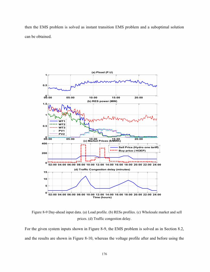
176
then the EMS problem is solved as instant transition EMS problem and a suboptimal solution
can be obtained.
Figure 8-9 Day-ahead input data. (a) Load profile. (b) RESs profiles. (c) Wholesale market and sell
prices. (d) Traffic congestion delay.
For the given system inputs shown in Figure 8-9, the EMS problem is solved as in Section 8.2,
and the results are shown in Figure 8-10, whereas the voltage profile after and before using the
00:00 05:00 10:00 15:00 20:000
0.5
1(a) Pload (P.U)
00:00 05:00 10:00 15:00 20:000
0.5
1
1.5(b) RES power (MW)
02:00 04:00 06:00 08:00 10:00 12:00 14:00 16:00 18:00 20:00 22:00 24:000
200
400(c) Market Prices ($/MWh)
02:00 04:00 06:00 08:00 10:00 12:00 14:00 16:00 18:00 20:00 22:00 24:000
5
10
15
Time (hours)
(d) Traffic Congestion delay (minutes)
WT1
WT2
WT3
PV1
PV2
Sell Price (Hydro one tariff)
Buy price ( HOEP)

177
MESS is depicted in Figure 8-11. The main objective is maximizing the DNO profit through
energy arbitrage and power loss minimization; thus as shown in Figure 8-10 (b), the MESS has
been charged during the lowest buy prices times (4-6 am) till reaching full capacity.
Table 8-1 Input data for the EMS.
RES Ratings 𝑝𝑊𝑇1 = 2𝑀𝑊, 𝑝𝑊𝑇2 = 1.5𝑀𝑊, 𝑝𝑊𝑇3 = 1.5𝑀𝑊,
𝑝𝑝𝑣1 = 0.5𝑀𝑊, 𝑝𝑝𝑣2 = 0.5𝑀𝑊, 𝑐𝐹𝐼𝑇 = 128 $/𝑀𝑊ℎ
Delay model 𝑑12 = 16.87 𝑘𝑚, 𝑑13 = 19.92 𝑘𝑚, 𝑑23 = 16.83 𝑘𝑚
𝑉𝑎𝑣𝑔 = 40𝑘𝑚 ℎ𝑟⁄ , 𝑡𝑖𝑛𝑠 = 5 𝑚𝑖𝑛𝑠. , 𝑇𝑠 = 10 𝑚𝑖𝑛𝑠.
EMS 𝑆𝑂𝐶0 = 0.5, 𝑆𝑂𝐶 = 0.2, 𝑁𝑡𝑟𝑖𝑝𝑠 = 3,𝑁 = 1
𝑣 = 0.95, 𝑣 = 1.05, 𝑁0 = 0, 𝜂𝑐ℎ = 0.75, 𝜂𝑑ℎ = 1.33
𝐹𝐶 = 0.4 $ 𝑘𝑚⁄ , 𝐶𝑘𝑤ℎ = 221 $ 𝑀𝑊ℎ⁄ , 𝑡𝑙𝑐 = 25 $ ℎ𝑟⁄
PSO 𝑀 = 30 𝑚𝑖𝑛𝑠. , 𝜔𝑚𝑎𝑥 = 0.9, 𝜔𝑚𝑖𝑛 = 0.1, 𝛼 = 2000,𝐶1 = 2, 𝐶2 = 2,𝓃 = 10
The MESS is partially discharged during the first price peak at 8 am. It continues being
charged at 9 am when the prices fall. It is worth mentioning that at 9 am; the battery is not
charged with full power as reactive power support is needed at this time to boost the voltage to
the minimum allowable level as depicted in the reactive power curve in Figure 8-10(b). Next, at
noon, where the second price peak exists, the MESS is fully discharged. After that, no
significate price difference exists that deserves another MESS charge and the state of charge is
settled at the minimum 20% level as in Figure 8-10(d). It should be noted that the price
difference should be at least greater than the charging cost 𝐶𝑘𝑤ℎ to make charging

178
economically viable (which does not happen again after 2 pm). Moreover, the number of cycles
allowed in this study is one; thus the total charged energy is less than the rated capacity and the
maximum number of cycle is less than one as in Figure 8-10(d). Finally, as the profit is the only
objective function here (energy arbitrage strategy), charging times are driven by the energy
price, unlike peak shaving whereas discharging hours are always located at peak hours. It is
noticed that the grid exported power is reduced during the high energy price as depicted in
Figure 8-10(c).
Regarding reactive power support, during late night, the power generated by wind turbines is
very high while the line is lightly loaded (see Figure 8-9). As a result, the voltage profile
increases above the limits (105%) during this time as shown in Figure 8-11, particularly in the
feeder end (bus 41). As a result, the first chosen location for the MESS is near these buses
(Station-3) as shown in Figure 8-10(a). During this time the energy price is minimal, and the
MESS is fully charged. In the morning (7-8 am), the MESS discharge during the first peak hour,
and then it changes its location to Station-1 (bus 9) where it recharges back (8-9 am). The
reason behind this location change is that charging at Station-1 (the nearest to grid) provides the
lowest power loss, further charging at Station-3 (bus 40) will lead to a further voltage drop at
the feeder end. The second transition occurs after charging as shown in Figure 8-10(a) when the
MESS goes back to Station-3 (bus 40) to discharge fully during the second peak hour (11 am-12
pm). After that, the SOC and number of cycles limits are reached as shown in Figure 8-10 (d),
thus zero active power is kept until the end of the day, however; the MESS keeps providing
reactive power support for keeping acceptable voltage limits. A final transition is made to
Station-2 around 2 pm. As noticed from Figure 8-10, the wind power plant (WT2) near Station-
2 drops to zero at the same time; thus a leading reactive power is needed at this far end feeder.
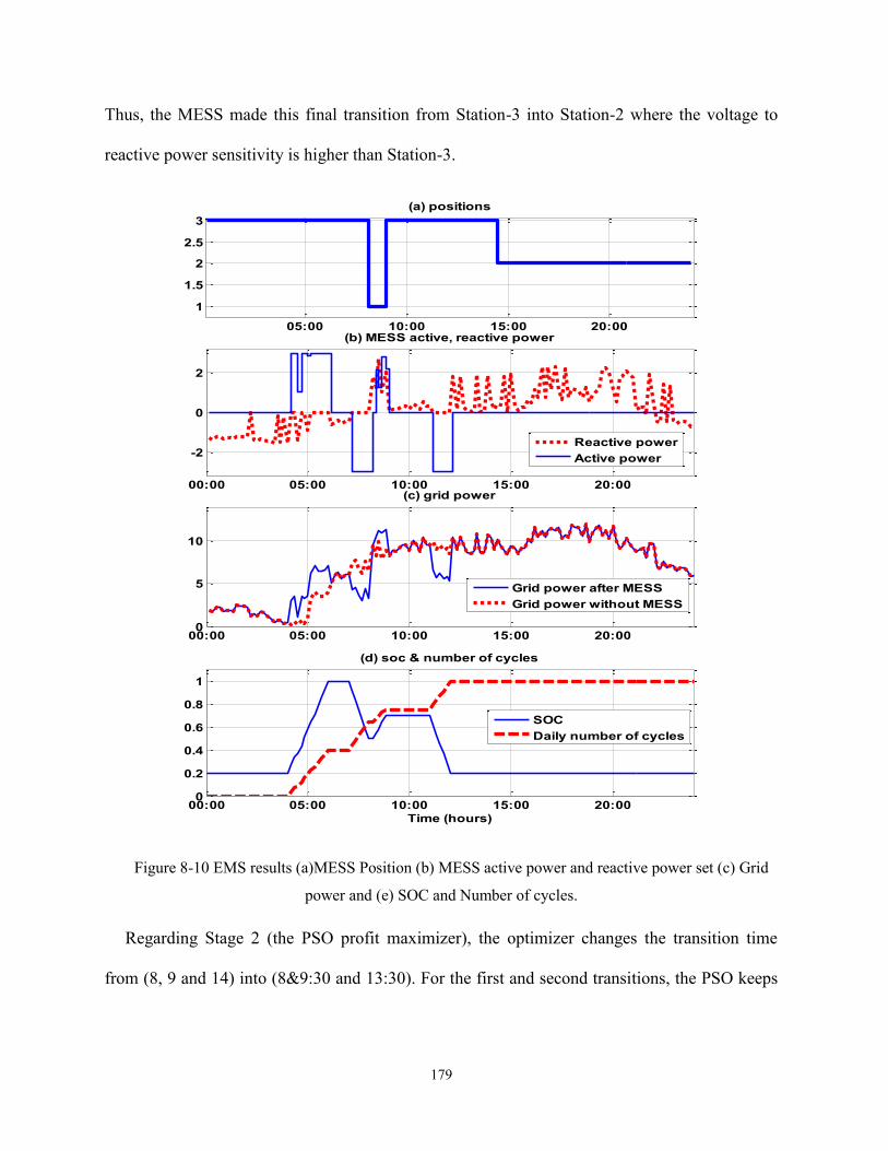
179
Thus, the MESS made this final transition from Station-3 into Station-2 where the voltage to
reactive power sensitivity is higher than Station-3.
Figure 8-10 EMS results (a)MESS Position (b) MESS active power and reactive power set (c) Grid
power and (e) SOC and Number of cycles.
Regarding Stage 2 (the PSO profit maximizer), the optimizer changes the transition time
from (8, 9 and 14) into (8&9:30 and 13:30). For the first and second transitions, the PSO keeps
05:00 10:00 15:00 20:00
1
1.5
2
2.5
3
(a) positions
00:00 05:00 10:00 15:00 20:00
-2
0
2
(b) MESS active, reactive power
00:00 05:00 10:00 15:00 20:000
5
10
(c) grid power
00:00 05:00 10:00 15:00 20:000
0.2
0.4
0.6
0.8
1
(d) soc & number of cycles
Time (hours)
Reactive power
Active power
Grid power after MESS
Grid power without MESS
SOC
Daily number of cycles

180
them the same as if the MESS left Station-3 earlier than 8 am, it will miss discharging during
the peak hour which will result in a big profit reduction.
For the second transition, if the MESS leaves Station-1 before 9 am, it will not be fully
charged which will reduce the profit in the future; however, if it stays longer at Station-1, the
traffic congestion delay will reduce from its 9 am peak as depicted in Figure 8-9 (d). Finally, for
the final transition (from Station-3 into Station-2), the PSO optimizer changes the transition
time from (2 pm into 1:30 pm) to end the ride (approximately 30 minutes ride with delays)
before the traffic congestion increases after 2 pm. It is worth mentioning that the PSO results
agree with the traffic delay profile in Figure 8-9 (d); thus, the PSO optimizes the transition
times to decrease the MESS delay and, therefore, maximizing its service period.
Figure 8-11 Voltage profile after and before using the MESS.
To sum up the results, Table 8-2 compares the techno-economic aspects after and before
using the MESS services (system with no storage at all and system that invests in an MESS).

181
Firstly, the MESS managed to provide a logistic localized reactive power support to keep the
voltage level within allowable limits which improves the power quality. Secondly, regarding
losses, the losses has been decreased by 5.5%. It is worth mentioning that the objective function
is the difference between the energy bought from the grid and that sold to loads. Thus the power
loss is inherently minimized in the objective function with a weight depending on the energy
prices at each instant. Thirdly, the net profit has increased by 3.1% as compared to that without
including the profit from the localized reactive power support that defers adding one or two
capacitor banks to this feeder.
Table 8-2 System performance comparison.
No MESS With MESS
Voltage level 𝑉𝑚𝑎𝑥 = 1.062, 𝑉𝑚𝑖𝑛 = 0.89
𝑉𝑚𝑎𝑥 = 1.04, 𝑉𝑚𝑖𝑛 = 0.956
Power loss 8.1863 𝑀𝑊ℎ 7.7277 𝑀𝑊ℎ
Profit 14,320$ 14,760$
Regarding enhancing the voltage profile, a good example appears when we focus on the
voltage at the worst case bus (bus-41) as shown in Figure 8-12. Bus 41 is a heavily loaded bus
(2.14 MW) with a big wind farm nearby (WT3 located in bus 40). Station-3 is located at bus 41.
However, the reactive power is injected at various stations according to Figure 8-10 (a).
As shown in Figure 8-12 (a), the wind power (WT3) exceeds bus-41 load till 5:00 am that
results in over voltage (as shown in Figure 8-12 (c)). Because an overvoltage occurs, the MESS
produces lagging reactive power from 0:00 till 4:00 (as shown in Figure 8-12 (c)) leading to
reducing the voltage magnitude to the allowable margin. Moving to hours 4:00 till 6:00, the
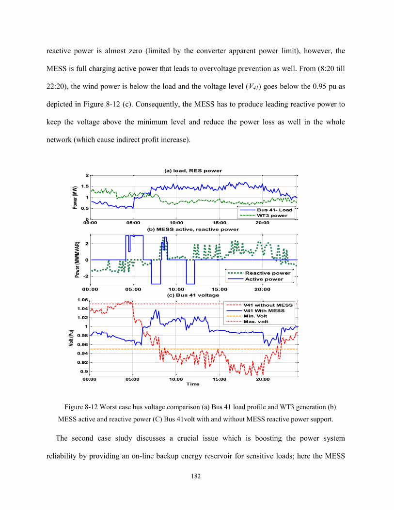
182
reactive power is almost zero (limited by the converter apparent power limit), however, the
MESS is full charging active power that leads to overvoltage prevention as well. From (8:20 till
22:20), the wind power is below the load and the voltage level (V41) goes below the 0.95 pu as
depicted in Figure 8-12 (c). Consequently, the MESS has to produce leading reactive power to
keep the voltage above the minimum level and reduce the power loss as well in the whole
network (which cause indirect profit increase).
Figure 8-12 Worst case bus voltage comparison (a) Bus 41 load profile and WT3 generation (b)
MESS active and reactive power (C) Bus 41volt with and without MESS reactive power support.
The second case study discusses a crucial issue which is boosting the power system
reliability by providing an on-line backup energy reservoir for sensitive loads; here the MESS
00:00 05:00 10:00 15:00 20:00
-2
0
2
(b) MESS active, reactive power
Pow
er (M
W/M
VAR
)
Reactive power
Active power
00:00 05:00 10:00 15:00 20:000
0.5
1
1.5
2
Pow
er (M
W)
(a) load, RES power
00:00 05:00 10:00 15:00 20:00
0.9
0.92
0.94
0.96
0.98
1
1.02
1.04
1.06
Time
Volt
(Pu)
(c) Bus 41 voltage
V41 without MESS
V41 With MESS
Min. Volt
Max. volt
Bus 41- Load
WT3 power
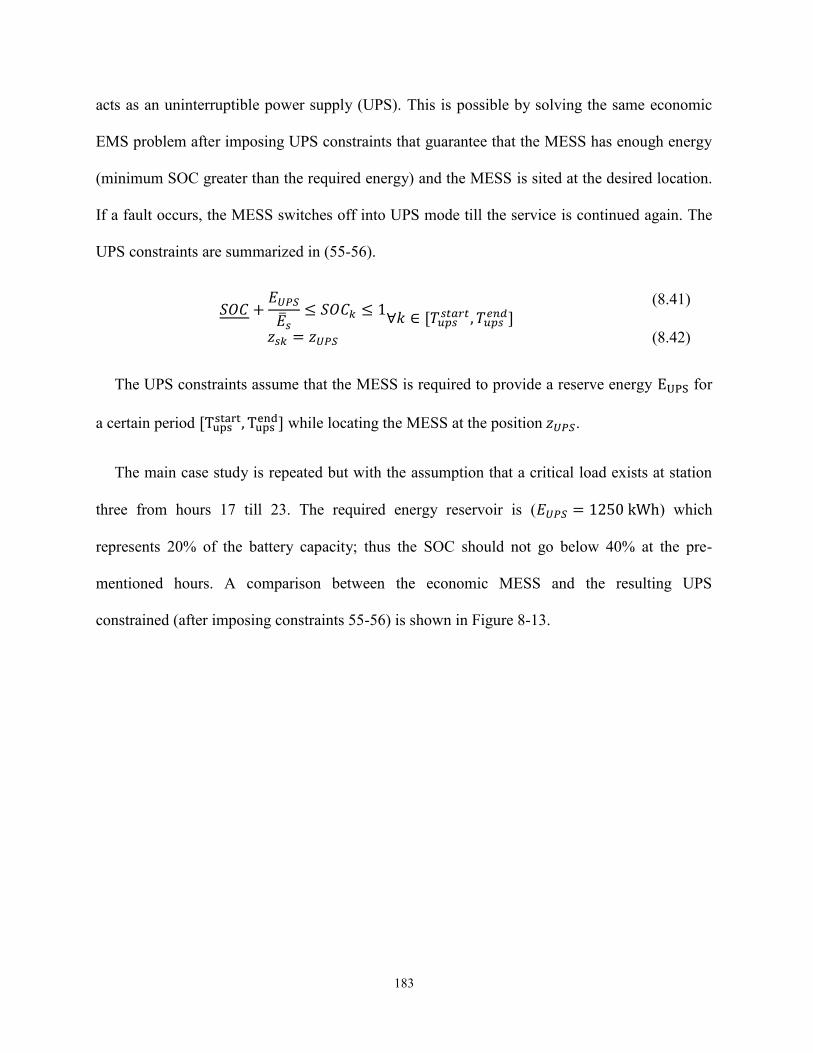
183
acts as an uninterruptible power supply (UPS). This is possible by solving the same economic
EMS problem after imposing UPS constraints that guarantee that the MESS has enough energy
(minimum SOC greater than the required energy) and the MESS is sited at the desired location.
If a fault occurs, the MESS switches off into UPS mode till the service is continued again. The
UPS constraints are summarized in (55-56).
𝑆𝑂𝐶 +𝐸𝑈𝑃𝑆
��𝑠≤ 𝑆𝑂𝐶𝑘 ≤ 1
𝑧𝑠𝑘 = 𝑧𝑈𝑃𝑆
∀𝑘 ∈ [𝑇𝑢𝑝𝑠𝑠𝑡𝑎𝑟𝑡 , 𝑇𝑢𝑝𝑠
𝑒𝑛𝑑] (8.41)
(8.42)
The UPS constraints assume that the MESS is required to provide a reserve energy EUPS for
a certain period [Tupsstart, Tups
end] while locating the MESS at the position 𝑧𝑈𝑃𝑆.
The main case study is repeated but with the assumption that a critical load exists at station
three from hours 17 till 23. The required energy reservoir is (𝐸𝑈𝑃𝑆 = 1250 kWh) which
represents 20% of the battery capacity; thus the SOC should not go below 40% at the pre-
mentioned hours. A comparison between the economic MESS and the resulting UPS
constrained (after imposing constraints 55-56) is shown in Figure 8-13.
184
Figure 8-13 Comparison between reliability-based EMS with economic EMS. (a) Station position of
MESS. (B) MESS state of charge.
In the UPS-constrained EMS, the MESS starts charging early to reach the required 40% SOC
by hour 17. At time 21:50, the main supply is disconnected, and the MESS starts acting as a
UPS till the service is resumed by 22:40. When the MESS returns again to the normal mode
after hour 23, it discharges the whole energy to go back to the minimum SOC of 20%. The
MESS has also stayed at Station-3 till hour 23; then it moved to Station-2 after (similar to the
economic EMS case).
Finally, it worth noticing that these results mainly depend on the market prices, the load and
RES profiles. Thus, in other days with no big market price difference, it is not economical to
operate the MESS [20]. Finally, Using the MESS in voltage support is optional in case of long
feeders where the transformer tap changer setting cannot guarantee an acceptable voltage at the
far end.
00:00 05:00 10:00 15:00 20:00
1
1.5
2
2.5
3
positions
00:00 05:00 10:00 15:00 20:000.2
0.3
0.4
0.5
0.6
0.7
0.8
0.9
1SOC
Time (hours)
Reliability-Constrainted EMS
Economic EMS

185
8.5 Conclusion
A day-ahead EMS for an MESS was presented in this chapter. The EMS objective function
aimed at maximizing the DNO day-ahead profit and regulating the voltage level. The proposed
EMS dispatched the MESS and allocated its station in the system. A traffic delay model was
developed between different stations. Using a two-stage optimization technique, firstly, the
problem was solved as a mixed-integer convex problem, and secondly, a PSO-based algorithm
was developed to optimize the transit times to maximize the profit. A case study on a real 41-
buses radial feeder with real data of RESs and loads was used to validate the results. The
proposed EMS successfully fulfilled all the optimization process objectives in an adaptive
manner that fitted the time-varying nature of renewable resources in modern active distribution
grids.

186
Chapter 9
9 Conclusions
9.1 Thesis Summary
This thesis discussed the optimal planning and energy management of energy storage
systems in the power system. The primary objective in both the planning and operation phases
was to maximize the profit of the owner (either a consumer or utility) while respecting the
different system technical constraints. To achieve these objectives, various optimization
techniques were utilized to guarantee feasible optimal decisions.
Different storage systems were investigated in this thesis (short and long period storage,
stationary and mobile storage). The thesis began investigating stationary storage planning in
Chapter 3. The planning scheme aimed at using ESSs for distribution system upgrade. ESS was
intended to provide multi-services by conducting T&D deferral, energy arbitrage, power loss
minimization and providing reactive power support, simultaneously. A case study using a real
radial feeder data is conducted. The results showed that energy arbitrage income was vital for a
viable ESS investment. Further, given the current market costs, NA-S battery was found to be a
competitive system upgrade option. Results also show that ESS was an effective upgrade tool
when sited at the feeder end close to big loads combined with SVCs (for reactive power
support) sited at the feeder start close to both big loads and/or RESs.

187
Chapter 4 discusses mobile energy storage planning in active distribution systems. To
achieve the same objectives as those in Chapter 3 (except for T&D deferral), a size-dependent
cost for the power converter was adopted in the planning process. The study results showed
that using the MESS may yield a higher profit than that yielded by stationary ESSs, due to its
low bulk power conversion cost.
Regarding operation phase, Chapter 5-8 focused on the energy management of different
storage systems. First, Chapter 5 presented a predictive EMS for a hybrid power system
(WECS with BESS). This EMS maximized the owner’s daily profit by dispatching the BESS
for wind energy time-shifting. To expand the BESS lifetime, constraints on the power rating,
the DOD and the number of charging cycles were included. This technique achieved the
optimal profit with a minimal sacrifice in the BESS lifetime guaranteeing the maximum net
profit.
Chapter 6 presented a predictive EMS for a short-term storage hybrid system. The system
consisting of a FESS connected with a WECS. The EMS used an MPC-based algorithm to
respect typical grid code, minimize the FESS losses, and increase the system lifetime. By
comparing the proposed EMS with a traditional EMS, the case studies show that the proposed
controller has managed to reduce the FESS losses up to 25%.
Chapter 7 presented a framework to define robust operating zones for multi-ESSs for day-
ahead. The technical constraints included permissible voltage level and branch ampacity. This
work c main contribution is to consider the power uncertainty while reducing the results
conservatism. When the ROZs were tested under different uncertainty scenarios, the results
showed that the proposed technique increased the ESS participation with a very low voltage and
ampacity violations.

188
Finally, Chapter 8 proposed a novel EMS for mobile storage. This EMS minimized the cost
of power imported from the grid and not only shifted renewable energy power to load peak
hours but also it provided localized reactive power support. The proposed EMS managed to
provide the optimal locations and dispatch power for an MESS which achieved a profit for the
utility, taking into account the truck transit delay.
9.2 Future work
The following research directions can be followed as an extension out of this thesis.
1) The utilization of ESSs in distribution system extension. Savings in the extension cost
can be achieved by reducing the feeders’ sizes in futuristic expansions; moreover, ESS-
multi-services enables reactive power support with the peak shaving process.
2) The application of the developed EMSs to hybrid systems with short and long duration
ESSs.
3) The inclusion of a detailed transit delay model in the planning process of MESSs.
4) The extension of the proposed planning and operation algorithms to multiple MESSs.
Whereas the ESS cost will decrease in the future, more ESSs are expected to join the power
systems for multi-services. This development will make all the suggested studies very useful for
viable control and sizing strategies for ESSs.
189
Bibliography
[1] S. Arefifar and Y. Mohamed, "DG Mix, Reactive Sources and Energy Storage Units for Optimizing Microgrid
Reliability and Supply Security," IEEE Transactions on smart Grid, vol. 5, no. 4, pp. 1835-1844, 2014.
[2] M. Arif, A. Oo and A. Ali, "Energy Storage: Applications and Advantages," in Smart Grids: Opportunities,
Developments, and Trends, New York, Springer, 2013, pp. 77-109.
[3] E. Jim and C. Garth, "Energy Storage for the Electricity Grid: Benefits and Market Potential Assessment
Guide," SANDIA, Albuquerque, New Mexico, 2010.
[4] R. Walawalkar and A. Jay, "Market Analysis of Emerging Electric Energy Storage Systems," NETL, 2008.
[5] LAZARD, "LAZARD's levelized cost of storage analysis- Version 1.0," LAZARD, November 2015.
[6] S. Chakraborty, T. Senjyu, H. Toyama, A. Saber and T. Funabashi, "Determination methodology for optimising
the energy storage size for power system," IET Generation, Transmission & Distribution, vol. 3, no. 11, pp.
987-999, 2009.
[7] H. Pandzic, Y. Wang, T. Qiu, Y. Dvorkin and D. Kirschen, "Near-Optimal Method for Siting and Sizing of
Distributed Storage in a Transmission Network," IEEE Trans. Power Syst., vol. 30, no. 5, pp. 2288-2300, 2015.
[8] S. Wogrin and D. Gayme, "Optimizing Storage Siting, Sizing, and Technology Portfolios in Transmission-
Constrained Networks," IEEE Trans. Power Syst., vol. 30, no. 6, pp. 3304-3313, 2015.
[9] M. Nick, R. Cherkaoui and M. Paolone, "Optimal Allocation of Dispersed Energy Storage Systems in Active
Distribution Networks for Energy Balance and Grid Support," IEEE Trans. Power Syst., vol. 29, no. 5, pp. 2300-
2310, 2014.
[10] S. Chen, H. Gooi and M. Wang, "Sizing of Energy Storage for Microgrids," IEEE Trans. Smart Grid, vol. 3, no.
1, pp. 142-151, Feb. 2012.
[11] C. Abbey and G. Joos, "A Stochastic Optimization Approach to Rating of Energy Storage Systems in Wind-
Diesel Isolated Grids," IEEE trans. Power Syst., vol. 24, no. 1, pp. 418-426, 2009.
[12] T. Nguyen, M. Crow and A. Elmore, "Optimal Sizing of a Vanadium Redox Battery System for Microgrid
Systems," IEEE Trans. Sust. Energy, vol. 6, no. 3, pp. 729-737, June 2015.
[13] Y. Makarov, P. Du, M. Meyer, C. Jin and H. Illian, "Sizing Energy Storage to Accommodate High Penetration
of Variable Energy Resources," IEEE Trans. Sust. Energy, vol. 3, no. 1, pp. 34-40, Jan. 2012.
[14] J. Xiao, L. Bai, F. Li, H. Liang and C. Wang, "Sizing of Energy Storage and Diesel Generators in an Isolated
Microgrid Using Discrete Fourier Transform (DFT)," IEEE Trans. Sust. Energy, vol. 5, no. 3, pp. 907-916,
2014.
[15] Y. Liu, W. Du, L. Xiao, H. Wang and J. Cao, "A Method for Sizing Energy Storage System to Increase Wind
Penetration as Limited by Grid Frequency Deviations," IEEE Trans. Power Syst., vol. pp, no. 99, pp. 1-9, 2015.
[16] Y. Liu, W. Du, L. Xiao, H. Wang, S. Bu and J. Cao, "Sizing a Hybrid Energy Storage System for Maintaining
Power Balance of an Isolated System With High Penetration of Wind Generation," IEEE Trans. Power Syst.,
vol. PP, no. 99, pp. 1-9, 2015.
[17] P. Li, R. Dargaville, F. Liu, J. Xia and Y. Song, "Data-Based Statistical Property Analyzing and Storage Sizing
for Hybrid Renewable Energy Systems," IEEE Trans. Indust. Electron., vol. 62, no. 11, pp. 6996-7008, 2015.
[18] S. Alnaser and L. Ochoa, "Optimal Sizing and Control of Energy Storage in Wind Power-Rich Distribution
Networks," IEEE Trans. Power Syst., vol. pp, no. 99, pp. 1-10, August 2015.
[19] X. Ke, N. Lu and C. Jin, "Control and Size Energy Storage Systems for Managing Energy Imbalance of
Variable Generation Resources," IEEE Trans. Sust. Energy, vol. 6, no. 1, pp. 70-78, Dec. 2015.
[20] H. Abdeltawab and Y. Mohamed, "Market-Oriented Energy Management of a Hybrid Wind-Battery Energy
Storage System Via Model Predictive Control With Constraint Optimizer," IEEE Trans. Indust. Electron., vol.
62, no. 11, pp. 6658-6670, 2015.
[21] S. Wen, H. Lan, Q. Fu, D. Yu and L. Zhang, "Economic Allocation for Energy Storage System Considering
190
Wind Power Distribution," IEEE Trans. Power Syst., vol. 30, no. 2, pp. 644-652, March 2015.
[22] H. Bludszuweit and J. Navarro, "A Probabilistic Method for Energy Storage Sizing Based on Wind Power
Forecast Uncertainty," IEEE Trans. Power Syst., vol. 26, no. 3, pp. 1651-1658, 2011.
[23] A. Awad, T. EL-Fouly and M. Salama, "Optimal ESS Allocation for Load Management Application," IEEE
Trans. Power Syst., vol. 30, no. 1, pp. 327-336, 2015.
[24] EPRI, "Transportable Energy Storage Systems Project," Oct 2009.
[25] D. Rastler, "Technical Specification for a Transportable Lithium-Ion Energy Storage System for Grid Support
Using Commercially Available Lithium- Ion Technology," EPRI, Jul 2012.
[26] winston-battery, "Mobile Power Storage," Winston Energy Group Limited, 2015. [Online]. Available:
http://en.winston-battery.com/index.php/products/mobile-power. [Accessed 30 July 2015].
[27] DOE, "Fujian Electric Power Research Institute Mobile Energy Storage Station I," Department of Energy,
[Online]. Available: http://www.energystorageexchange.org/projects/153. [Accessed 30 July 2015].
[28] Toshiba, "Spain’s Gas Natural Fenosa and Toshiba to Demonstrate Use of Transportable Lithium-ion Battery
Energy Storage System in Power Distribution Network," Toshiba, 2014. [Online]. Available:
https://www.toshiba.co.jp/about/press/2014_01/pr0704.htm. [Accessed 30 July 2015].
[29] Y. Zheng, D. Zhaoyang, S. Huang, M. Ke, L. Fengji, J. Huang and H. David, "Optimal integration of mobile
battery energy storage in distribution system with renewables," Journal of Modern Power Systems and Clean
Energy, vol. 3, no. 4, pp. 589-596, 2015.
[30] E. Perez, H. Beltran, N. Aparicio and P. Rodriguez, "Predictive Power Control for PV Plants With Energy
Storage," IEEE Trans. Sustainable Energy, vol. 4, no. 2, pp. 482-490, 2013.
[31] A. Gabash and P. Li, "Flexible Optimal Operation of Battery Storage Systems for Energy Supply Networks,"
IEEE Trans. Power Syst., vol. PP, no. 99, pp. 1-10, 2012.
[32] S. Wang and Y. Liu, "A PSO-Based Fuzzy-Controlled Searching for the Optimal Charge Pattern of Li-Ion
Batteries," IEEE Trans. Ind. Electron., vol. 62, no. 5, pp. 2983- 2993, 2015.
[33] J. Trovao, V. Santos, C. Henggeler, P. Pereirinha and H. Jorge, "A Real-Time Energy Management Architecture
for Multisource Electric Vehicles," IEEE Trans. Ind. Electron., vol. 62, no. 5, pp. 3223-3233, 2015.
[34] X. Lu, K. Sun, J. Guerrero, J. Vasquez and L. Huang, "State-of-Charge Balance Using Adaptive Droop Control
for Distributed Energy Storage Systems in DC Microgrid Applications," IEEE Trans. Ind. Electron., vol. 61, no.
6, pp. 2804- 2815, 2014.
[35] J. Talla, L. Streit, Z. Peroutka and P. Drabek, "Position-Based T-S Fuzzy Power Management for Tram With
Energy Storage System," IEEE Transactions on Industrial Electronics, vol. 62, no. 5, pp. 3061- 3071 , 2015.
[36] S. Teleke, M. Baran, S. Bhattacharya and A. Huang, "Optimal Control of Battery Energy Storage for Wind Farm
Dispatching," IEEE Trans. Energy Convers., vol. 25, no. 3, pp. 787-794, 2010.
[37] W. Qi, J. Liu and P. Christofides, "Distributed Supervisory Predictive Control of Distributed Wind and Solar
Energy Systems," IEEE Trans. Control Syst. Technol., vol. 21, no. 2, pp. 504-512, 2013.
[38] P. Poonpun and W. Jewell, "Analysis of the Cost per Kilowatt Hour to Store Electricity," IEEE Trans. Energy
Convers., vol. 23, no. 2, pp. 529-534, 2008.
[39] L. Y and P. Flynn, "Deregulated Power prices: comparison of Volatility," Energy Policy, vol. 32, no. 14, pp.
1591-1601, 2004.
[40] D. Rastle, "Electricity Energy Storage Technology Options," ELECTRIC POWER RESEARCH INSTITUTE ,
Palo Alto, California, 2010.
[41] S. Vazquez, S. Lukic, E. Galvan, L. Franquelo and J. Carrasco, "Energy Storage Systems for Transport and Grid
Applications," IEEE Trans. Ind. Electron., vol. 57, no. 12, pp. 3881-3895, 2010.
[42] R. Arghandeh, M. Pipattanasomporn and S. Rahman, "Flywheel Energy Storage Systems for Ride-through
Applications in a Facility Microgrid," IEEE Trans. Smart Grid, vol. 3, no. 4, pp. 1955-1962, 2012.
[43] Y. Suzuki, A. Koyanagi, M. Kobayashi and R. Shimada, "Novel applications of the flywheel energy storage
system," Energy, vol. 30, no. 11-12, pp. 2128-2143, Aug. 2005.
[44] L. H and J. J, "Flywheel energy storage—An upswing technology for energy sustainability," Energy and
buildings, vol. 39, pp. 599-604, 2007.
191
[45] S. Samineni, B. Johnson, H. Hess and J. Law, "Modeling and analysis of a flywheel energy storage system for
Voltage sag correction," IEEE Trans. Ind. Appl., vol. 42, no. 1, pp. 42-52, Jan. 2006.
[46] B. power, "Beacon power," 2014. [Online]. Available: http://beaconpower.com/. [Accessed 30 September
2014].
[47] X. Chang, Y. Li, W. Zhang, N. Wang and W. Xue, "Active Disturbance Rejection Control for a Flywheel
Energy Storage System," IEEE Trans. Ind. Electron., vol. 62, no. 2, pp. 991-1001, Feb. 2015.
[48] C. Jin, N. Lu, S. Lu, Y. Makarov and R. Dougal, "A Coordinating Algorithm for Dispatching Regulation
Services Between Slow and Fast Power Regulating Resources," IEEE Trans. Smart Grid, vol. 5, no. 2, pp. 1043-
1050, 2014.
[49] N. Lu, F. Rudolph and C. loutan, "THE WIDE-AREA ENERGY STORAGE AND MANAGEMENT SYSTEM
PHASE II," PNNL, Richland, Washington, 2010.
[50] G. Thijissen and J. Enslin, "Cost Comparison for a 20 MW Flywheel-based Frequency Regulation Power Plant,"
KEMA, Raleigh, NC, 2007.
[51] temporal, "temporal power," 2014. [Online]. Available: http://temporalpower.com/. [Accessed 30 September
2014].
[52] R. Sebastian and A. R., "Flywheel energy storage systems: Review and simulation for an isolated wind power
system," Renewable and Sustainable Energy Reviews, vol. 16, pp. 6803-6813, Dec. 2012.
[53] D. Francisc, S. Andreas, G. Oriol and D. Fernando, "Energy management of flywheel-based energy storage
device for wind power smoothing," Applied Energy, vol. 110, p. 207–219, 2013.
[54] G. Suvire, M. Molina and P. Mercado, "Improving the Integration of Wind Power Generation Into AC
Microgrids Using Flywheel Energy Storage," IEEE Trans. Smart Grid, vol. 3, no. 4, pp. 1945-1954, 2012.
[55] K. Z. and V. I., "Losses of flywheel energy storages and joint operation with solar cells," Journal of Materials
Processing Technology, vol. 161, pp. 62-65, 2005.
[56] D. Gerada, A. Mebarki, N. Brown, C. Gerada, A. Cavagnino and A. Boglietti, "High-Speed Electrical Machines:
Technologies, Trends, and Developments," IEEE Trans. Ind. Electron., vol. 61, no. 6, pp. 2946 - 2959, June
2014.
[57] R. Cardenas, R. Pena, G. Asher, J. Clare and R. Blasco-Gimenez, "Control strategies for power smoothing using
a flywheel driven by a sensorless vector-controlled induction machine operating in a wide speed range," IEEE
Trans. Ind. Electron., vol. 51, no. 3, pp. 603-614, 2004.
[58] J. Beno, R. Thompson, M. Werst, S. Manifold and J. Zierer, "End-of-life design for composite rotors [flywheel
systems]," IEEE Trans. Magn., vol. 37, no. 1, pp. 284-289, 2001.
[59] S. Arnold, A. Saleeb and N. Al-Zoubi, "Deformation and life analysis of composite flywheel disk systems,"
Composites Part B: Engineering, vol. 33, pp. 433-459, 2002.
[60] F. Islam, A. Al-Durra and S. Muyeen, "Smoothing of Wind Farm Output by Prediction and Supervisory-
Control-Unit-Based FESS," IEEE Trans. Sust. Energy, vol. 4, no. 4, pp. 925-933, Oct. 2013.
[61] J. Chen and M. Goloshchapova, "Energy Storage Initiative Issue Identification," AESO, Edmonton, 2013.
[62] A. Gabash and P. Li, "Active-Reactive Optimal Power Flow in Distribution Networks With Embedded
Generation and Battery Storage," IEEE Trans. Power Syst., vol. 27, no. 4, pp. 2026-2035, 2012.
[63] D. Gayme and U. Topcu, "Optimal power flow with large-scale storage integration," IEEE Trans. Power Syst.,
vol. 28, no. 2, pp. 709-717, 2013.
[64] Y. Levron, J. Guerrero and Y. Beck, "Optimal Power Flow in Microgrids With Energy Storage," IEEE Trans.
Power Syst., vol. 28, no. 3, pp. 3226-3234, 2013.
[65] A. Gabash and P. Li, "Flexible Optimal Operation of Battery Storage Systems for Energy Supply Networks,"
IEEE Transactions on Power Systems, vol. 28, no. 3, pp. 2788-2797, 2013.
[66] H. Akhavan-Hejazi and H. Mohsenian-Rad, "Optimal Operation of Independent Storage Systems in Energy and
Reserve Markets With High Wind Penetration," IEEE Trans. Smart Grid, vol. 5, no. 2, pp. 1088-1097, 2014.
[67] S. Nykamp, M. Bosman, A. Molderink, J. Hurink and G. Smit, "Value of Storage in Distribution Grids—
Competition or Cooperation of Stakeholders?," IEEE Trans. Smart Grid, vol. 4, no. 3, pp. 1361-1370, 2013.
[68] A. Oudalov, D. Chartouni and C. Ohler, "Optimizing a Battery Energy Storage System for Primary Frequency
Control," IEEE Trans. Power Syst., vol. 22, no. 3, pp. 1259-1266, 2007.
192
[69] H. Oh, "Optimal Planning to Include Storage Devices in Power Systems," IEEE Trans. Power Syst., vol. 26, no.
3, pp. 1118-1128, 2011.
[70] J. Tant, F. Geth, D. Six, P. Tant and J. Driesen, "Multiobjective Battery Storage to Improve PV Integration in
Residential Distribution Grids," IEEE Transactions on Sustainable Energy, vol. 4, no. 1, pp. 182-191, 2013.
[71] Z. Shu and P. Jirutitijaroen, "Optimal Operation Strategy of Energy Storage System for Grid-Connected Wind
Power Plants," IEEE Trans Sust. Energy, vol. 5, no. 1, pp. 190-199, 2014.
[72] C. Martinez, E. Bonvallet, R. Behnke and X.-P. Zhang, "Impacts of Energy Storage on Short Term Operation
Planning Under Centralized Spot Markets," IEEE Trans. Smart Grid, vol. 5, no. 2, pp. 1110-1118, 2014.
[73] M. Khodayar, L. Wu and M. Shahidehpour, "Hourly Coordination of Electric Vehicle Operation and Volatile
Wind Power Generation in SCUC," IEEE Transactions on Smart Grid, vol. 3, no. 3, pp. 1271-1279, 2012.
[74] D. Bertsimas, E. Litvinov, X. Sun, J. Zhao and T. Zheng, "Adaptive Robust Optimization for the Security
Constrained Unit Commitment Problem," IEEE Trans. Power Syst., vol. 28, no. 1, pp. 52-63, 2013.
[75] R. Jiang, J. Wang and Y. Guan, "Robust Unit Commitment With Wind Power and Pumped Storage Hydro,"
IEEE Trans. Power Syst., vol. 27, no. 2, pp. 800-810, 2012.
[76] C. Zhao, J. Wang, J. Watson and Y. Guan, "Multi-Stage Robust Unit Commitment Considering Wind and
Demand Response Uncertainties," IEEE Transactions on Power Systems, vol. 28, no. 3, pp. 2708-2717, 2013.
[77] Y. Zhang, N. Gatsis and G. Giannakis, "Robust Energy Management for Microgrids With High-Penetration
Renewables," IEEE Trans. Sust. Energy, vol. 4, no. 4, p. 2013, 944-953.
[78] Q. Wang, J. Watson and Y. Guan, "Two-stage robust optimization for N-k contingency-constrained unit
commitment," IEEE Trans.Power Syst., vol. 28, no. 3, pp. 2366-2375, 2013.
[79] Y. Guan and J. Wang, "Uncertainty Sets for Robust Unit Commitment," IEEE Trans. Power Syst., vol. pp, no.
99, pp. 1-2, 2013.
[80] Y. Liu, C. Yuen, N. Hassan, S. Huang, R. Yu and S. Xie, "Electricity Cost Minimization for a Microgrid With
Distributed Energy Resource Under Different Information Availability," IEEE Trans. Indust. Electron., vol. 62,
no. 4, pp. 2571-2583, 2015.
[81] R. Yu, W. Zhong, S. Xie, C. Yuen, S. Gjessing and Y. Zhang, "Balancing Power Demand Through EV Mobility
in Vehicle-to-Grid Mobile Energy Networks," IEEE Trans. Indust. Informat., vol. 12, no. 1, pp. 79-90, 2016.
[82] K. W. Hu and C. M. Liaw, "Incorporated Operation Control of DC Microgrid and Electric Vehicle," IEEE
Trans. Ind Elect, vol. 63, no. 1, pp. 202-215, 2016.
[83] W. Tushar, C. Yuen, S. Huang, D. Smith and H. Poor, "Cost Minimization of Charging Stations With
Photovoltaics: An Approach With EV Classification," IEEE Trans. Intell Trans Syst, vol. 17, no. 1, pp. 156-169,
2016.
[84] P. Sanchez, G. Sanchez and G. Morales, "Direct Load Control Decision Model for Aggregated EV Charging
Points," IEEE Trans Power Syst., vol. 27, no. 3, pp. 1577-1584, 2012.
[85] R. Bessa and M. Matos, "Optimization Models for EV Aggregator Participation in a Manual Reserve Market,"
IEEE Tran Power Syst, vol. 28, no. 3, pp. 3085-3095, 2013.
[86] J. Eyer, "Electric Utility Transmission and Distribution Upgrade Deferral Benefits from Modular Electricity
Storage," Sandia National Laboratories, Albuquerque, New Mexico, June 2009.
[87] M. Carrion and J. Arroyo, "A Computationally Efficient Mixed-Integer Linear Formulation for the Thermal Unit
Commitment Problem," IEEE Trans. Power Syst., vol. 21, no. 3, pp. 1371-1378, 2006.
[88] L. Gan, N. Li, U. Topcu and S. Low, "Exact Convex Relaxation of Optimal Power Flow in Radial Networks,"
IEEE Trans. Power Syst., vol. 60, no. 1, pp. 72-87, 2015.
[89] J. Lavaei, D. Tse and B. Zhang, "Geometry of Power Flows and Optimization," IEEE Trans. Power Syst., vol.
29, no. 2, pp. 572-583, 2014.
[90] W. Shi, X. Xie, C. Chu and R. Gadh, "Distributed Optimal Energy Management in Microgrids," IEEE Trans.
Smart Grid, vol. 6, no. 3, pp. 1137-1146, 2015.
[91] K. Christakou, J. LeBoudec, M. Paolone and D. Tomozei, "Efficient Computation of Sensitivity Coefficients of
Node Voltages and Line Currents in Unbalanced Radial Electrical Distribution Networks," IEEE Trans. Smart
Grid, vol. 4, no. 2, pp. 741-750, June 2013.
[92] M. Hong, "An Approximate Method for Loss Sensitivity Calculation in Unbalanced Distribution Systems,"
193
IEEE Trans. Power Syst., vol. 29, no. 3, pp. 1435-1436, May 2014.
[93] S. Lee and S. Yang, "Derivation of P-Q Loss Sensitivities by Angle Reference Transposition and an Application
to Optimal P-Q Generation for Minimum Cost," IEEE Trans. Power Syst., vol. 21, no. 1, pp. 428-430, Feb.
2006.
[94] Y. Atwa, "Distribution System Planning and Reliability Assessment under High DG Penetration," University of
Waterloo, Waterloo, Ontario, Canada, 2010.
[95] PJM, "meterd load data," 2015. [Online]. Available: http://www.pjm.com/markets-and-operations/ops-
analysis/historical-load-data.aspx. [Accessed 1 December 2015].
[96] SODA, "Solar Energy Services for Professionals," 2015. [Online]. Available: http://www.soda-
is.com/eng/index.html. [Accessed 1 Dec. 2015].
[97] A. E. S. Operator, "Wind power data," 2016. [Online]. Available:
http://www.aeso.ca/gridoperations/20544.html. [Accessed 1 Dec. 2015].
[98] I. E. S. Operato, "Power data of IESO," 2016. [Online]. Available: http://www.ieso.ca/Pages/Power-
Data/default.aspx#download.
[99] N. Pattani, "Transmission & Distribution Considerations For Distributed Generation," Hydro One, January,
2009.
[100] S. Schoenung, "Energy Storage Systems Cost Update; A Study for the DOE Energy Storage Systems Program,"
Sandia National Laboratories , Albuquerque, New Mexico, April 2011.
[101] N. Mukherjee and D. Strickland, "Second life battery energy storage systems: Converter topology and
redundancy selection," in PEMID 2014, 2014.
[102] Gurobi, "Gurobi Optimization," Shell, [Online]. Available: http://www.gurobi.com/. [Accessed 18 Aug 2015].
[103] I. R. E. Agency, "Battery Storage For Renewables; Market Status And Technology Outlook," IRENA, 2015.
[104] Y. Amirnasr and I. Reza, Voltage-Sourced Converters in Power Systems, Wiley, 2010.
[105] D. Rastler, A. Akhil, D. Gauntlett and C. E, "Energy Storage System Costs 2011 update, Executive Summary,"
EPRI, Feb., 2012.
[106] J. Kennedy and R. Eberhart, "Particle Swarm Optimization," in IEEE International Conference on Neural
Networks, 1995.
[107] A. E. S. Operator, "Market & System Reporting," AESO, [Online]. Available:
http://www.aeso.ca/market/8856.html.
[108] AESO, 2015. [Online]. Available: http://www.aeso.ca/gridoperations/20544.html.
[109] AESO, 2015. [Online]. Available: http://www.aeso.ca/market/23873.html.
[110] EPCOR, 2015. [Online]. Available: http://www.epcor.com/power-natural-gas/regulated-rate-
option/Pages/residential-rates.aspx.
[111] F. Valenciaga, P. Puleston, P. Battaiotto and R. Mantz, "Passivity/sliding mode control of a stand-alone hybrid
generation system," IEE Proceedings - Control Theory and Applications, vol. 147, no. 6, pp. 680-686, 2000.
[112] D. Lee and L. Wang, "Small-Signal Stability Analysis of an Autonomous Hybrid Renewable Energy Power
Generation/Energy Storage System Part I: Time-Domain Simulations," IEEE Transactions on Energy
Conversion,, vol. 23, no. 1, pp. 311-320, 2008.
[113] I. S. C. C. 2. o. S. Batteries, IEEE Recommended Practice for Sizing Lead-Acid Batteries for Stationary
Applications, IEEE, 1997.
[114] J. Jiang, Q. Liu, C. Zhang and W. Zhang, "Evaluation of Acceptable Charging Current of Power Li-Ion Batteries
Based on Polarization Characteristics," IEEE Trans Indust. Electron., vol. 61, no. 12, pp. 6844- 6851, 2014.
[115] M. Ceraolo, "New dynamical models of lead-acid batteries," IEEE Transactions on Power Systems, vol. 15, no.
4, pp. 1184-1190, 2000.
[116] M. Gholizadeh and F. Salmasi, "Estimation of State of Charge, Unknown Nonlinearities, and State of Health of
a Lithium-Ion Battery Based on a Comprehensive Unobservable Model," IEEE Trans Indust. Electron., vol. 61,
no. 3, pp. 1335- 1344, 2014.
[117] j. Ayoub, L. Dignard-Bailey and Y. Poissant, "exchange and dissemination of information on pv power
systems," canmetENERGY, Varennes, Quebec, 2011.
194
[118] Y. Li and P. Flynn, "Deregulated power prices: changes over time," IEEE Trans Power Syst., vol. 20, no. 2, pp.
565-572, 2005.
[119] AESO, "Implementation of Market & Operational Framework For Wind Integration in Alberta," 2009.
[120] AESO, "Wind power Management Protocol for Alberta," AESO, 2008.
[121] C. Zhou, K. Qian, M. Allan and W. Zhou, "Modeling of the Cost of EV Battery Wear Due to V2G Application
in Power Systems," IEEE Trans. Energy Convers., vol. 26, no. 4, pp. 1041-1050, 2011.
[122] D. Jenkins, J. Fletcher and D. Kane, "Lifetime prediction and sizing of lead-acid batteries for microgeneration
storage applications," IET Renewable Power Generation, vol. 2, no. 3, pp. 191-200, 2008.
[123] L. Wang, Model control systems design and implementation Using Matlab, Springer, 2008.
[124] S. Vazquez, J. Leon, L. Franquelo, J. Rodriguez, H. Young, A. Marquez and P. Zanchetta, "Model Predictive
Control: A Review of Its Applications in Power Electronics," IEEE Industrial Electronics Magazine, vol. 8, no.
1, pp. 16-31, 2014.
[125] AESO, "historical pool price for Alberta," 2000. [Online]. Available: http://ets.aeso.ca/. [Accessed MAY 2013].
[126] M. Tsili and S. Papathanassiou, "A review of grid code technical requirements for wind farms," IET Renewable
Power Generation, vol. 3, no. 3, pp. 308- 332 , 2009.
[127] S. Kim, S. Bae, Y. Kang and J. Park, "Energy Management Based on the Photovoltaic HPCS With an Energy
Storage Device," IEEE. Trans. Ind. Electron., vol. 62, no. 7, pp. 4608 - 4617, July 2015.
[128] K. Keesman, System Identification; An Introduction, Springer, 2011.
[129] AESO, "AESO Recommendation paper (Implementation of Market & Operational Framework for Wind
Integration in Alberta)," Alberta energy system operator, Edmonton, 2009.
[130] B. Jonkman and L. Kilcher, "TurbSim User's Guide: Version 1.0600," NREL, Golden, Colorado, Sept., 2012.
[131] R. Gagnon, B. Saulnier and A. Forcione, "mathworks," 2015. [Online]. Available:
http://www.mathworks.com/examples/simpower/105-wind-farm-dfig-phasor-model. [Accessed 12 August
2015].
[132] V. Marandi, L. Pak and V. Dinavahi, "Real-Time Simulation of Grid-Connected Wind Farms Using Physical
Aggregation," IEEE Trans. Indust. Electron., vol. 57, no. 9, pp. 3010-3021, 2010.
[133] W. Li, G. Joos and J. Belanger, "Real-Time Simulation of a Wind Turbine Generator Coupled With a Battery
Supercapacitor Energy Storage System," IEEE Trans. Indust. Electron., vol. 57, no. 4, pp. 1137-1145, 2010.
[134] J. Jung, S. Ahmed and P. Enjeti, "PEM Fuel Cell Stack Model Development for Real-Time Simulation
Applications," IEEE Trans. Indust. Electron., vol. 58, no. 9, pp. 4217-4231, 2011.
[135] A. Thatte, L. Xie, D. Viassolo and S. Singh, "Risk Measure Based Robust Bidding Strategy for Arbitrage Using
a Wind Farm and Energy Storage," IEEE Trans. Smart Grid, vol. 4, no. 4, pp. 2191-2199, 2013.
[136] w. Pedrycz and f. Gomide, Fuzzy Systems Engineering Toward Human-Centric Computing, Wiley, 2007.
[137] W. Li, J. Zhou, K. Xie and X. Xiong, "Power System Risk Assessment Using a Hybrid Method of Fuzzy Set and
Monte Carlo Simulatio," IEEE Transactions on Power Systems , vol. 23, no. 2, pp. 336-343, 2008.
[138] D. Popovic and Z. Popovic, "A risk management procedure for supply restoration in distribution networks,"
IEEE Trans. Power Syst., vol. 19, no. 1, pp. 221-228, 2004.
[139] A. Almeida, E. Valenca de Lorenci, R. Leme, A. Zambroni de Souza, B. Lopes and K. Lo, "Probabilistic voltage
stability assessment considering renewable sources with the help of the PV and QV curves," IET Renewable
Power Generation, vol. 7, no. 5, pp. 521- 530, 2013.
[140] M. AlRashidi and M. El-Hawary, "Hybrid Particle Swarm Optimization Approach for Solving the Discrete OPF
Problem Considering the Valve Loading Effects," IEEE Transactions on Power Systems, vol. 22, no. 4, pp.
2030-2038, 2007.
[141] A. Esmin, G. Torres and A. de Souza, "A hybrid particle swarm optimization applied to loss power
minimization," IEEE Trans. Power Syst., vol. 20, no. 2, pp. 859-866, 2005.
[142] Y. Chakhchoukh, P. Panciatici and L. Mili, "Electric Load Forecasting Based on Statistical Robust Methods,"
IEEE Trans. Power Syst., vol. 26, no. 3, pp. 982-991, 2011.
[143] D. Saez, F. Avila, D. Olivares, C. Canizares and L. Marin, "Fuzzy Prediction Interval Models for Forecasting
Renewable Resources and Loads in Microgrids," IEEE Trans. Smart Grid, vol. 6, no. 2, pp. 548-556, 2015.

195
[144] "Winston Energy Group Limited," [Online]. Available: http://en.winston-
battery.com/index.php/products/mobile-power. [Accessed 30 July 2015].
[145] I. Cambridge Systematics, "Traffic Congestion and Reliability (Trends and Advanced Strategies for Congestion
Mitigation)," Federal Highway Administration , Sept. 2005.
[146] IESO, "feed in tariff," [Online]. Available: http://fit.powerauthority.on.ca/. [Accessed 8 Sept. 2015].
[147] H. One, "electricity Rates," [Online]. Available:
http://www.hydroone.com/MyHome/MyAccount/UnderstandMyBill/Pages/ElectricityRates.aspx. [Accessed 23
Aug. 2015].
[148] IESO, "Price schedule," IESO, [Online]. Available: http://fit.powerauthority.on.ca/program-resources/price-
schedule. [Accessed 08 Sept. 2015].
[149] Alibaba, "30 ton tow truck," ALibaba.com, [Online]. Available:
https://www.alibaba.com/trade/search?fsb=y&IndexArea=product_en&CatId=&SearchText=30+ton+tow+truck.
[Accessed 25 May 2016].
[150] T. G. o. Ontario, "Traveller Information Services 2015," [Online]. Available:
http://www.mto.gov.on.ca/english/traveller/trip/traffic_reports.shtml. [Accessed 28 March 2016].
[151] E. Perez, H. Beltran, N. Aparicio and P. Rodriguez, "Predictive Power Control for PV Plants With Energy
Storage," IEEE Trans. Sust. Energy, vol. 4, no. 2, pp. 482-490, 2013.