Planned Developments in California: Private … Developments in California: Private Communities and Public Life ••• Tracy M. Gordon 2004

PlannedDevelopments inCalifornia: PrivateCommunities and Public Life

• • •

Tracy M. Gordon

2004

Library of Congress Cataloging-in-Publication DataGordon, Tracy M.Planned developments in California : private communities and

public life / Tracy M. Gordon.p. cm.

ISBN: 1-58213-081-71. Planned communities—California. 2. Housing, Cooperative—

California. 3. Condominium associations—California. 4. Homeowners’ associations—California. 5. California—Ethnic relations. 6. Social classes—California. 7. Political participation—California. 8. Voting—California. I. Title.

HT167.5.C2G57 2004307.76'8'09794—dc22 2004001904

Research publications reflect the views of the authors and do notnecessarily reflect the views of the staff, officers, or Board ofDirectors of the Public Policy Institute of California.

Copyright © 2004 by Public Policy Institute of CaliforniaAll rights reservedSan Francisco, CA

Short sections of text, not to exceed three paragraphs, may be quotedwithout written permission provided that full attribution is given to

the source and the above copyright notice is included.

PPIC does not take or support positions on any ballot measure or onany local, state, or federal legislation, nor does it endorse, support, oroppose any political parties or candidates for public office.

iii

Foreword

Over the last three decades, there has been a notable increase incommon interest developments (CIDs) in California. Variouslycharacterized as “Fortress America,” “privatopias,” “secession of thesuccessful,” or, more neutrally, “private government,” CIDs in thebroadest sense (condominiums, cooperatives, and planned developments)now make up 60 percent of new housing starts in California. However,the image of CIDs commonly projected in critical scholarship andjournalism is the gated suburban community closed to public access.These communities provide an array of traditional public servicesthrough private, commonly held organizations governed by theirresidents. The most extreme characterizations suggest that CIDs arenothing less than income and racial segregation reinvented in a moremodern, legal form. Less extreme characterizations suggest that suchcommunities might well signal an effective withdrawal of residents fromtraditional civic society—contributing to declining voting rates and thegeneral movement toward fiscal conservatism at the state and local levelsof government.

PPIC research fellow Tracy Gordon has taken a careful look atCIDs as an increasingly popular form of privatization. In PlannedDevelopments in California: Private Communities and Public Life,Gordon focuses primarily on planned developments, the prevalent formof CIDs in California. Drawing on a unique dataset of real estate activityin California, she concludes that some “sorting” is apparent whenresidents of planned developments are compared to other residents incentral cities and suburbs. Residents in planned developments have ahigher percentage of non-Hispanic whites, higher incomes, and moreeducation and they are generally older than the comparison group. Herfindings hold up even when she looks at planned developments forcentral cities and suburbia separately. The concern over social andeconomic segregation is thus given some support by the report. She is

iv

careful to note, however, that the contribution of planned developmentsto overall residential segregation is minor, and she found little evidencethat residents of planned developments are withdrawing from civic life—at least as measured by voting behavior.

It is striking that condominiums have also grown in importance tothe new homebuyer—representing 37 percent of all CIDs in Californiacompared to 61 percent for planned developments. Althoughcondominiums are often seen as the first rung in the ladder of eventualhome ownership, they are also fraught with challenges whendisagreements arise between developers and owners and later on whenowners cannot agree on key common interest issues. In a review of thegovernance processes used by CIDs, Gordon notes that the definition ofcommunity varies from example to example, but managing a communityinterest may be just as difficult as reaching a decision in local planningcommission meetings.

In sum, CIDs are here to stay, and Gordon has made a valuablecontribution to our understanding of them in California. AlthoughCIDs are still a relatively small part of the overall housing stock inCalifornia, their steep growth path and tendency toward residentialselectivity suggest that they are well worth monitoring in the years anddecades ahead. De Tocqueville’s observation that America has apenchant for voluntary associations may now be evolving into yetanother form—voluntary local government imposed by the decision topurchase a home. This is certainly not a new idea, but this latest exampleserves as a reminder of the challenges facing California’s governingprocesses at various levels.

David W. LyonPresident and CEOPublic Policy Institute of California

v

Summary

Nearly three million California homes, one-quarter of the statehousing stock, are located within common interest developments (CIDs)such as planned developments, condominiums, and cooperatives.Moreover, this proportion is ever-increasing, with CIDs accounting for60 percent of residential construction starts during the 1990s. One typeof CID, the planned development, alone represented more than 40percent of new single-family home sales over this period (see Figure S.1).

More than a pattern of residential development, CIDs are anemerging form of privatization. Homeowner associations in CIDsprovide many goods and services traditionally supplied by localgovernment, including garbage collection, street cleaning, street lighting,and security patrol. They also levy assessments, adjudicate disputes, andregulate land use as well as other aspects of life within their boundaries.As a result, CIDs are often called “quasi-” or “private governments.”

0

500

1,000

1,500

2,000

2,500

Hou

sing

uni

ts (

1000

s)

CondominiumsCooperativesPlanned developments

SOURCE: HOA-Info (2002).NOTE: Figure does not include CIDs of unknown type.

1960 1970 1975 1980 1985 1990 1995 2000

Figure S.1—Growth of Common Interest Developments in California

vi

The growth of so-called private governments has sparked a populardebate. Proponents claim that CIDs aid cash-strapped localities inaccommodating the service and infrastructure costs of growth. Theyfurther advocate extending this governance structure to existingneighborhoods as a means of improving local amenities andneighborhood quality. Critics charge that CIDs generate adverseconsequences for nonresidents. Primary among these feared outcomes isheightened racial and economic segregation and diminished civicengagement.

Such criticisms have prompted recurrent calls for enhancedregulation of these communities. Although the bulk of proposedlegislation has addressed the internal governance of CIDs, a frequentcomplaint is that there are no current and reliable studies of commoninterest developments in California. In 1999, for example, the statelegislature authorized the California Law Revision Commission toundertake a multiyear investigation to address, among other questions,“to what extent [common interest housing developments] should besubject to regulation” (California Law Revision Commission, 2001, p. 3).

This report seeks to fill the gap in knowledge about CIDs inCalifornia. It focuses on planned developments, in particular, becausethese are the most prevalent and fastest-growing type of CID in bothCalifornia and the nation as a whole. These developments also bear thestrongest resemblance to traditional local government and hence attractthe most scrutiny for their potential policy consequences.

A Large and Diverse GroupThere are over 36,000 common interest developments in California.

These communities range in size from three to 30,000 units and canaccommodate several different housing types and legal ownershipstructures. The majority of CID units (61 percent) are located inplanned developments, in which each homeowner owns his or herindividual unit and lot and a homeowner association owns and maintainsall common property. The other major type of CID (37 percent of allunits) is the condominium, in which each owner holds title to his or herindividual unit and a percentage interest in the common areas.

vii

Monthly assessments in CIDs vary widely, from merely nominalamounts to thousands of dollars per unit per month. In 2002, medianmonthly assessments were $112 per unit in planned developments and$186 per unit in condominiums and cooperatives. Total homeownerassociation revenues in California were estimated at $6.3 billion in 2003(HOA-Info, 2003).

Successful But Not SecedingSocial commentators have referred to the spread of CIDs as the

“secession of the successful” (Reich, 1991). An examination of thedemographic and socioeconomic composition of planned developmentslends support to this view. Nevertheless, the data also suggest that thepicture is more complicated.

Planned developments are less diverse with respect to race andethnicity than other neighborhoods. In both central city and suburbanareas, planned developments include significantly more residents who arenon-Hispanic white (60 and 65 percent) and fewer who are black (4percent in central cities and 3 percent in suburban areas) and Hispanic(20 and 19 percent, respectively). Interestingly, suburban planneddevelopments tend to have larger Asian populations than otherneighborhoods (Table S.1).

Residents of planned developments are on average older than othercentral city or suburban dwellers. Planned developments include moreindividuals age 65 and over than other neighborhoods (differences of 2 to3 percentage points, depending on location). They also include moreresidents ages 40 to 64 (differences of 3 and 4 percentage points forcentral cities and suburbs, respectively). Planned developments havecorrespondingly smaller population shares in the younger age categoriesand slightly fewer married couples with children (Table S.2).

Planned developments are more diverse with respect to income thantheir image might suggest. To be sure, planned developments housemore of the highest-income Californians than other neighborhoods. Incentral cities and suburbs, 22 and 26 percent of planned developmenthouseholds earned more than $100,000 in 1999, compared to 15 to 17percent of households in other neighborhoods. However, planneddevelopments also include nearly as many residents in the middle- to

viii

Table S.1

Selected Demographic Characteristics of California Planned Developments(in percent)

Central City Suburb Characteristic

PlannedDevelopments

Non-PDNeighborhoods

PlannedDevelopments

Non-PDNeighborhoods

Black 4.2 9.8** 2.7 5.1**Hispanic 20.1 33.5** 18.8 32.6**Asian 11.7 12.3 10.3 9.2**White 60.2 40.8** 64.6 49.5**Age 0 to 19 25.1 28.3** 27.0 30.3**Age 20 to 39 30.2 33.2** 26.1 28.7**Age 40 to 64 30.7 27.6** 33.6 29.6**Age 65 and up 14.0 10.9** 13.3 11.4**

SOURCES: HOA-Info (2002); U.S. Census Bureau (2002a).

NOTE: Table includes sample means for each subgroup.

**Denotes statistically significant difference at the 1 percent level.

higher-income categories ($35,000 to $49,999, $50,000 to $74,999, and$75,000 to $99,999) as do other neighborhoods (Table S.2).

Despite their relative racial and ethnic homogeneity, thecontribution of planned developments to residential segregation is minor.Differences between planned developments and other neighborhoodsaccount for only 2 percent of statewide metropolitan area segregation.This finding is primarily due to the relatively small proportion of thepopulation living within planned developments. Although theyrepresent roughly 40 percent of new single-family homes, planneddevelopments constitute only 12 percent of the existing housing stock.

Planned developments do not exhibit markedly different patterns ofvoting behavior once other relevant characteristics are taken into account.At first glance, planned developments have higher rates of voterregistration and turnout than other neighborhoods. They also appearmore likely to affiliate with the Republican Party and to vote forstatewide ballot propositions favoring the privatization of governmentservices (Propositions 35 and 38) and higher vote requirements for feesand bonds (Propositions 37 and 39).

ix

Table S.2

Selected Socioeconomic Characteristics of California Planned Developments

Central City Suburb

CharacteristicPlanned

DevelopmentsNon-PD

NeighborhoodsPlanned

DevelopmentsNon-PD

NeighborhoodsMedian household

income in 1999, $ 58,687.8 46,688.3** 67,045.9 53,297.9**Household income, %

Less than $35,000 32.9 42.9** 26.8 35.6**$35,000–$49,999 14.2 15.0** 13.7 15.5**$50,000–$74,999 19.1 17.5** 19.8 20.1$75,000–$99,999 12.4 10.0** 13.5 12.0**$100,000–$199,999 16.6 11.6** 19.5 13.5**$200,000 and up 4.9 3.0** 6.6 3.3**

% Married coupleswith children 30.9 31.9** 34.4 36.4*

% with no college 28.0 40.4** 26.5 38.8**% in managerial and

professionaloccupations 42.6 33.8** 42.3 32.4**



*Denotes statistically significant difference at the 5 percent level.


However, planned developments also differ from otherneighborhoods along a number of dimensions that are related to votingbehavior (e.g., age, income, education, and residential mobility).Regression analyses holding these differences constant demonstrate thatplanned developments themselves do not strongly affect either politicalparticipation or patterns of voting behavior in statewide general elections.Remaining differences are small, at 1 to 2 percentage points.

These conclusions are somewhat unexpected. Thus far, it wouldappear that concerns about planned developments siphoning off thewealthiest Californians and their participation in public life areunwarranted. Planned developments still represent a relatively smallproportion of the population overall, however, and as their numbersincrease, their effects on neighborhood composition and civicengagement may become more pronounced.

xi

Contents

Foreword..................................... iiiSummary..................................... vFigures ...................................... xiiiTables....................................... xvAcknowledgments ............................... xix

1. INTRODUCTION........................... 1

2. WHAT ARE COMMON INTERESTDEVELOPMENTS? .......................... 9A Brief History .............................. 9Definition and Taxonomy ....................... 11Scope of Activities ............................ 13Policy Issues ................................ 14

3. WHAT DO CALIFORNIA CIDs LOOK LIKE? ........ 19Note on Data Sources .......................... 19A Large and Diverse Group ...................... 20

4. FOCUS ON PLANNED DEVELOPMENTS.......... 27Geographic Distribution ........................ 27Demographic and Socioeconomic Characteristics ........ 28Diversity and Segregation ....................... 35

5. VOTING BEHAVIOR ........................ 39Voter Turnout, Registration, and Party Affiliation ........ 41Voting on Statewide Ballot Propositions .............. 41A Closer Look at Voting Behavior .................. 42

6. CONCLUSIONS ............................ 49

AppendixA. Data and Methods ............................ 51B. Measuring Diversity and Segregation ................ 55C. Technical Considerations and Regression Results ........ 61

xii

References .................................... 73

About the Authors ............................... 79

Related PPIC Publications.......................... 81

xiii

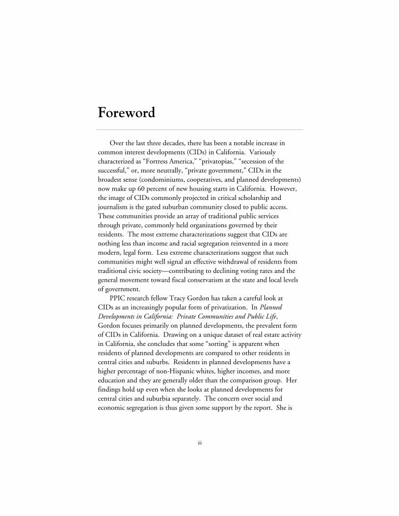
Figures

S.1. Growth of Common Interest Developments inCalifornia ............................... v

1.1. Growth of Common Interest Develoments in the UnitedStates.................................. 2

1.2. Growth of Common Interest Developments andSuburban Housing Units in California and the UnitedStates, 1940–1999 ......................... 4

2.1. Growth of Common Interest Developments in theUnited States, by Type....................... 12

3.1. Growth of Common Interest Developments inCalifornia, by Type......................... 22

3.2. Size Distribution of Common Interest Developments inCalifornia, by Type......................... 23

3.3. Revenues of Common Interest Developments inCalifornia ............................... 25

5.1. Estimated Effects of Planned Developments on VoterTurnout, Registration, and Party Affiliation ......... 45

5.2. Estimated Effects of Planned Developments on Votes forStatewide Ballot Propositions .................. 47

A.1. Example of Geocoding Procedure................ 52

xv

Tables

S.1. Selected Demographic Characteristics of CaliforniaPlanned Developments ...................... viii

S.2. Selected Socioeconomic Characteristics of CaliforniaPlanned Developments ...................... ix

2.1. An Example of Nonterritorial and Territorial CIDs .... 122.2. Services Provided by Common Interest Developments in

the United States and California ................ 133.1. Geographic Distribution of Common Interest

Developments ............................ 213.2. Types of Common Interest Developments in

California ............................... 223.3. Average Size of Common Interest Developments, by

Year of Construction ........................ 233.4. Distribution of Monthly Fees of Common Interest

Developments ............................ 244.1. Planned Developments, by Region ............... 284.2. Planned Developments, by Central City/Suburban

Location and Incorporation Status ............... 294.3. Planned Developments, by City Size and City

Incorporation Date ......................... 294.4. Selected Demographic Characteristics of California

Planned Developments ...................... 304.5. Selected Socioeconomic Characteristics of California

Planned Developments ...................... 314.6. Selected Housing Characteristics of California Planned

Developments ............................ 324.7. Percentage Black, by Planned Development Status and

Housing Characteristics ...................... 334.8. Percentage Hispanic, by Planned Development Status

and Housing Characteristics ................... 34

xvi

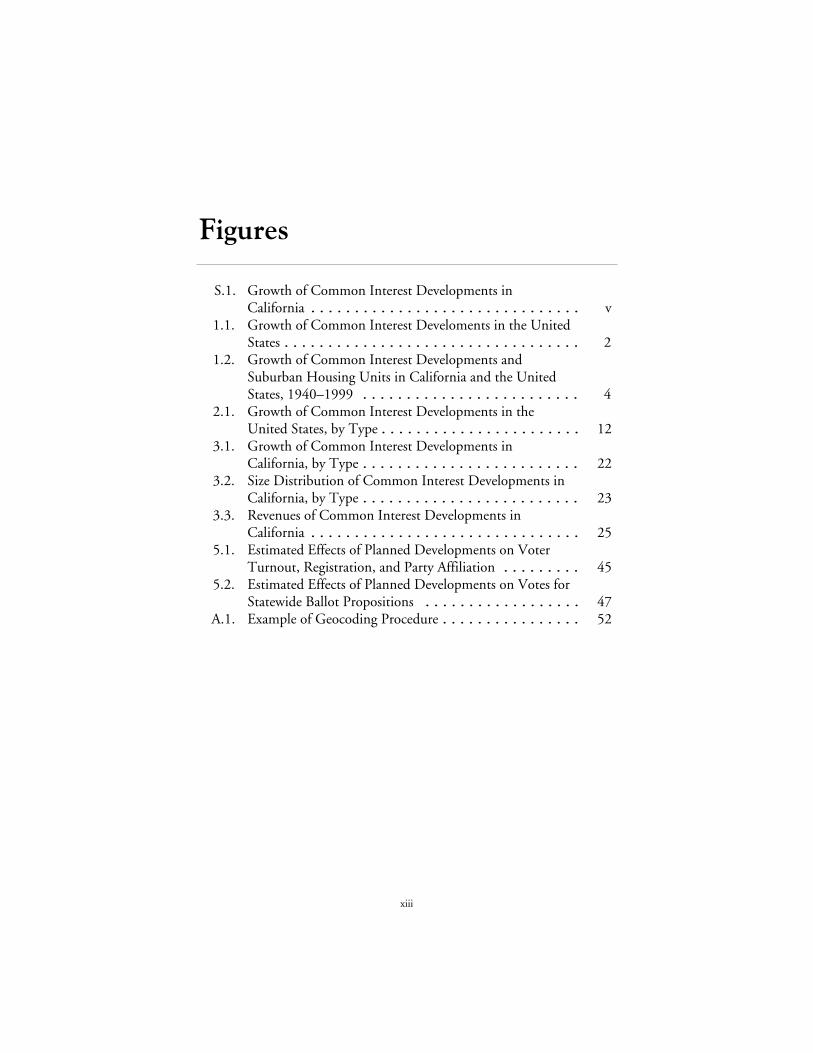
4.9. Average Diversity Scores of California Neighborhoods,by Metropolitan Area, Planned Development, andCentral City/Suburban Status .................. 36

4.10. Decomposition of Statewide Metropolitan RacialSegregation .............................. 37

5.1. Voter Turnout and Party Affiliation, by PlannedDevelopment Status ........................ 42

5.2. Approval Rates for Statewide Ballot Propositions, byPlanned Development Status................... 43

5.3. Summary of Demographic and SocioeconomicDifferences Between Planned Developments and OtherNeighborhoods and Predicted Effects on VoterTurnout ................................ 44

5.4. Voter Turnout, by Planned Development Status andRacial and Ethnic Diversity.................... 44

5.5. Voter Registration, by Planned Development Status andRacial and Ethnic Diversity.................... 45

A.1. Selected Characteristics of Planned Developments inCalifornia ............................... 53

A.2. Regional Distribution of Planned Developments Units,by Sample Definition ....................... 54

B.1. Decomposition of Segregation, by Planned Developmentand Central City/Suburban Status ............... 56

C.1. Estimated Effects of Planned Developments on VoterTurnout, 2000............................ 62

C.2. Estimated Effects of Planned Developments onPercentage Registered, 2000 ................... 63

C.3. Estimated Effects of Planned Developments onPercentage Registered Democrat, 2000 ............ 64

C.4. Estimated Effects of Planned Developments onPercentage Registered Republican, 2000 ........... 65

C.5. Estimated Effects of Planned Developments onPercentage Registered Independent, 2000........... 66

C.6. Estimated Effects of Planned Developments on “Yes”Votes for Proposition 32, 2000 ................. 67


xvii




xix

Acknowledgments

This report benefited from the contributions of several individuals.David Levy of Levy & Company, CPAs, generously provided access tothe HOA-Info dataset and shared his extensive knowledge of the CIDindustry. Julia Lave-Johnston and Dean Misczynski of the CaliforniaResearch Bureau, Peter Detwiler of the Senate Local GovernmentCommittee, J. Stacey Sullivan of the Assembly Local GovernmentCommittee, and Nathaniel Sterling of the California Law RevisionCommision shed light on legal and policy issues relating to CIDs.Professor Robert Jay Dilger of West Virginia University, David Levy,and Paul Lewis, Christopher Weare, and Junfu Zhang of PPIC gavethoughful reviews of the initial manuscript. Joyce Peterson, PeterRichardson, and Patricia Bedrosian improved the clarity of exposition.David Haskel and Rachel Flood provided excellent research assistance.Any remaining errors, as well as opinions or interpretations expressed inthis report, are those of the author alone and do not reflect the views ofthe Public Policy Institute of California.

1

1. Introduction

Rancho Bernardo, a master-planned community located about 25miles north of downtown San Diego, houses approximately 45,000residents in a mix of single-family detached homes, townhouses,condominiums, and apartments. The community also features serviceand retail businesses, light industry, shopping areas, parks, and golfcourses. Council members elected from districts oversee workingcommittees on public safety, government relations, utilities, traffic,transportation, finance, services, and elections. A planning boardenforces land use codes, and a recreation council maintains thecommunity park.

Although it bears a striking resemblance to a city, Rancho Bernardois in fact a private corporation. It is a large, but by no means unusual,example of what has been called “the most significant privatization oflocal government responsibilities in recent times” (Advisory Commissionon Intergovernmental Relations, 1989, p. 18). It also represents a shiftin the usual concept of privatization. In contrast to previous models,where a government contracts with a private firm for the provision of asingle service or function, individuals today are increasingly contractingdirectly with so-called “private governments” for many, if not all,traditional municipal services. According to one study, this trendrepresents nothing less than “a quiet revolution,” with profoundimplications for community organization, local government, land use,neighbor relations, and other aspects of public life (Barton andSilverman, 1994, p. xi).

Rancho Bernardo is an example of a common interest development,or CID.1 Common interest developments encompass several housing____________

1Common interest developments are also known as community associations (CAs),common interest communities (CICs), common interest realty associations (CIRAs), andresidential community associations (RCAs) (Treese, 1999, p. 3). A related phenomenonis the business or downtown improvement district (BID or DID) (Pack, 1992).

2

types and ownership structures, including planned developments,condominiums, and cooperatives. The distinguishing feature of thesecommunities is common property ownership. Beyond an individualhouse or unit, property owners in these communities also hold aninterest in common areas—such as recreation facilities, streets, lawns, orparking lots—either as individuals or through a mandatory homeownerassociation. Deed restrictions known as conditions, covenants, andrestrictions (CCRs) authorize the association to collect lien-basedassessments in exchange for providing services and regulating land use aswell as other aspects of life within CID boundaries.

Over the past 30 years, common interest developments haveproliferated throughout the United States. In 1962, there were fewerthan 500 common interest developments nationally; today there arenearly 250,000 CIDs housing an estimated 50 million Americans andconstituting 15 percent of the U.S. housing stock (CommunityAssociations Institute, 2003) (Figure 1.1).2

CIDs as a % of total housing unitsTotal CIDs

0

50

100

150

200

250

Num

ber

of C

IDs

(100

0s)

0

2

4

6

8

10

12

14

16

CID

s as

a %

of t

otal

uni

ts

SOURCE: Treese (1999).

1962 1970 1975 1980 1985 1990 1995 1999

Figure 1.1—Growth of Common Interest Developments in the United States

____________ 2Gated communities constitute a subset of this total. The Community Associations

Institute (CAI) estimates that 19 percent of its members, or 8.4 million people, livewithin gated communities (Blakely and Snyder, 1997, p. 3). Other sources put thisfigure at four million people, or roughly 10 percent of all CID residents (Egan, 1995, pp.A1, A22). The CAI estimate is likely an upper bound because its members tend to belarger associations.

3

In California, these trends are pronounced: There are three millionhomes within common interest developments, encompassing nearly one-quarter of the state housing stock. Moreover, CIDs constituted 60percent of new construction starts during the 1990s (HOA-Info, 2002;U.S. Census Bureau, 1994, 1995, 1996, 1998, 1999, 2002b). Planneddevelopments alone represent over 40 percent of new single-family homesales in the state (Construction Industry Research Board, 2000).

To put this trend in perspective, compare the growth of CIDs to thetrend of suburbanization more generally. Since 1970, common interestdevelopments have grown faster than the suburbs as a share of all housingunits in both California and the United States (Figure 1.2). This growthrate exceeds the pace of suburbanization during the peak years of 1940 to1960 by a factor of five.3 Although a vast literature has explored thesocial, economic, and political implications of suburbanization, theconsequences of this most recent transformation are largely unknown.

The growth of common interest developments has nonethelesssparked a popular debate. Proponents claim that CIDs aid cash-strappedlocalities in meeting demand for public services.4 They further advocateextending this governance structure to existing neighborhoods as a wayto improve local amenities and neighborhood quality (e.g., Nelson,1999; Ellickson, 1998). Critics charge that common interestdevelopments have adverse consequences for nonresidents. Primaryamong these feared outcomes is heightened racial and economicsegregation. Robert Reich (1991), for example, has referred to thegrowth of CIDs as the “secession of the successful.” Similarly, EvanMcKenzie (1994), in his comprehensive study of the rise of CIDs, linksthe CCRs governing these communities to the history of exclusionaryzoning practices in the United States. Although the Supreme Courtruled in 1948 that racially restrictive covenants were illegal (Shelley v.Kraemer), McKenzie argues “the principle is still the same: certain____________

3The average annual growth rates for each type of housing share in each period were10 and 2 percent, respectively.

4In theory, common interest developments may also improve efficiency in theallocation of public goods by allowing individuals to “vote with their feet” among anexpanded array of public and private options for funding and receiving collective services(e.g., Tiebout, 1956).

4

United States

0

10

20

30

40

50S

ubur

ban

hous

ing

as a

% o

f tot

al u

nits

Sub

urba

n ho

usin

g as

a%

of t

otal

uni

ts

0

2

4

6

8

10

12

14

16

CID

s as

a %

of t

otal

uni

tsC

IDs

as a

% o

f tot

al u

nits

0

10

20

30

40

50

60

0

5

10

15

20

25

1940 1960 1975 1990

California

CID unitsSuburb units

SOURCE: Treese (1999); HOA-Info (2002); Devaney (1994); U.S. Census Bureau (1970, 1980, and 1990).

1940 1950 1960 1970 1980 1990

Figure 1.2—Growth of Common Interest Developments and SuburbanHousing Units in California and the United States, 1940–1999

groups of people are considered a threat to property values and areexcluded. The result is still increased homogeneity and . . . continuingracial segregation” (p. 78).

Other social commentators have expressed concern about the effectsof CIDs on political participation and civic engagement. Robert Putnam(2000, p. 210), for instance, links the growth of CIDs to declines insocial capital:

Not only are canvassing politicians and Girl Scouts selling cookies excludedfrom exclusive communities, but the affluent residents themselves also appearto have a surprisingly low rate of civic engagement and neighborliness evenwithin their boundaries.

One reason to expect lower rates of political participation in CIDs isthat the homogeneity of these communities reduces the incentives, or

5

controversies, that draw citizens into civic affairs (Oliver, 2001).5

Alternatively, if planned developments are substitutes for traditional localgovernment, then residents of these developments may perceive lessbenefit to taking part in elections and other aspects of public life. Forinstance, in their survey of gated communities in particular, Blakely andSnyder assert that residents of these developments “have less need toparticipate [in the wider community] . . . because they live in gatedenclaves, with private recreation, roads, parks, and security” (1997, p.72).

A related concern is that members of common interest developmentsmay vote differently from nonmembers. In particular, CID residents mayfavor public spending that complements private expenditures (e.g., policeprotection) but oppose that which is duplicative (e.g., infrastructure) orredistributive (e.g., welfare). Simply put (“Government by the Nice . . . ,”1992, p. 25):

If affluent Americans choose to live in private communities which raise theirown taxes but do not redistribute them outside their walls, they are likely tovote to cut spending on public services that they do not use, ignoring the needsof people who cannot afford to go private.

Such criticisms have promoted repeated calls for enhanced regulationof these communities. Over the years, the state legislature has convenedseveral committees and working groups to review policies towardcommon interest developments. Although the bulk of proposedlegislation has focused on the internal governance of CIDs, a frequentcomplaint is that there are no current and reliable studies of commoninterest developments in California (e.g., Senate Housing andCommunity Development Committee, 2002; California Law RevisionCommission, 2002a). A California Research Bureau reportcommissioned by the Senate Housing and Land Use Committeerecommended a new legislative subcommittee “to provide more up-to-date empirical research on [homeowner associations] and related issues”(Roland, 1998, p. 44).____________

5See Alesina and La Ferrara (2000) for an opposing view, i.e., that heterogeneitydepresses participation in voluntary associations.

6

The primary reason for the lack of empirical research on CIDs islimited data. The federal government only recently began collectinginformation on gated communities and residential associations in its2001 American Housing Survey. As a result, most research on commoninterest developments has relied on small-scale surveys and case studies(e.g., McKenzie, 1994; Foldvary, 1994; Blakely and Snyder, 1997), withthe exception of Barton and Silverman (1994) whose results, based on a1987 survey, are largely out of date.

Given the absence of research in this area, there is a great deal ofuncertainty regarding common interest developments among state andlocal lawmakers, policy analysts, and CID managers and otherprofessionals, boards of directors, and residents themselves. An improvedunderstanding of these communities is an important prerequisite to theformation of sound policies toward private government. This reportseeks to fill the gap in knowledge about common interest developmentsin California. It focuses on planned developments, in particular, becausethese are the most prevalent and fastest-growing type of CID in bothCalifornia and the nation as a whole. These developments also representthe closest analogue to traditional local government and hence thegreatest source of controversy regarding common interest developments.

Among the questions addressed in this report are:

• What are common interest developments? What types ofhousing structures do they include? What kinds of services dothey provide? How are they similar to and different fromtraditional local governments?

• What do common interest developments in California look like?How many CIDs are there? How are they distributedregionally? How do they vary in type, size, age, and financialresources?

• What about planned developments in particular? Where arethey located? How do they compare to other neighborhoods interms of their demographic and socioeconomic characteristics(e.g., racial and ethnic composition, age structure, incomedistribution)? Do they contribute to overall residentialsegregation?

7

• Do planned developments represent the “secession of thesuccessful”? Do these communities exhibit lower levels of civicengagement, as measured by rates of voter turnout andregistration? Do they have a different political ideology, asindicated through party affiliation and votes on statewide ballotpropositions?

The plan for the remainder of the report is as follows. Chapter 2compares the origins, institutional features, and powers andresponsibilities of common interest developments to traditional localgovernment. Chapter 3 presents a portrait of common interestdevelopments in California, highlighting the diversity among thesecommunities. Chapter 4 analyzes the demographic and socioeconomiccomposition of planned developments, in particular, and theircontribution to overall residential segregation. Chapter 5 compares voterturnout and patterns of voting behavior in planned developments tosimilar neighborhoods, using regression analysis to control for relevantdemographic and socioeconomic factors. Chapter 6 concludes and offersdirections for state and local public policy.

9

2. What Are Common InterestDevelopments?

This chapter presents an overview of common interest developmentsin the United States. It traces the evolution of these communities fromEbenezer Howard’s “garden cities of tomorrow” to the modern CID.The chapter also develops a definition and taxonomy of common interestdevelopments. It concludes with a discussion of the scope of activities ofthese so-called “private governments” and issues for policymakers.

A Brief HistoryAlexis de Tocqueville observed that the principle of voluntary

association had nowhere in the world “been more successfully used, orunsparingly applied to a multitude of different objects, than in America.”He further described these associations as “a separate nation in the midstof the nation, a government within the government” (1969 [1835], pp.513–517). Yet the idea of residential associations based on collectiveproperty ownership originated in England. During the mid-1700s, LordLeicester established a park in Leicester Square and charged adjacentproperty owners an assessment for their exclusive enjoyment of it. In1837, private developers built Victoria Park, a community with deedrestrictions tied to the sale of each lot to protect local amenities(Foldvary, 2002, p. 274).

Perhaps the most important antecedent to the modern commoninterest development was Ebenezer Howard’s utopian ideal of the gardencity. Howard sought to combine the best aspects of city and country lifein his “new towns” of Welwyn and Letchworth, England. Both citieswere based on a leasehold concept, whereby a group of trustees wouldown the municipality and collect rents from its residents to pay off initialconstruction loans, build infrastructure, and provide collective services.Howard characterized the political organization as a technocracy,

10

“‘modelled upon that of a large and well-appointed business.’” In hisview, this governance structure would be more powerful than other localbodies and “‘solve to a large extent the problem of local self-government’” (McKenzie, 1994, pp. 5–6).

Precursors to the CID in the United States—Gramercy Park in NewYork City (established in 1831), Louisburg Square in Boston (1844), andSouth Park in San Francisco (1852)—were formed primarily to maintainprivate amenities. Builder Jesse Clyde Nichols established the first full-service common interest development, Mission Hills, Missouri, in 1914with the express intention of supplanting local government. Accordingto one study, “he was afraid if the subdivision were part of a larger villageor town organization the political unit would not be sufficientlyresponsive to the needs of his residents” (Worley, 1990, pp. 166–167).During the 1920s, the reform-minded Regional Planning Association ofAmerica revived the idea of a “garden city” with the new town ofRadburn, New Jersey. In addition to its innovative physical plan, thecommunity included a homeowner association with broad land useregulation and service responsibilities (Barton and Silverman, 1994,p. 9).

The popularity of common interest developments burgeoned duringthe post–World War II housing boom and rise of “community builders,”who favored large-scale, dense forms of development. In 1961 and 1963,the Federal Housing Administration encouraged this form of housing bypublishing guidelines for condominiums and planned developments toobtain mortgage insurance. The Federal National Mortgage Associationand Federal Home Loan Mortgage Corporation later approvedcondominium and planned development purchases for secondarymortgage loan markets. State and local governments also codified realestate practices and modified building and zoning laws in the 1960s toaccommodate CID housing.1 This period of growth culminated in theemergence of large-scale master-planned communities such as Irvine,California, and Reston, Virginia.____________

1For instance, many localities implemented planned unit development (PUD)zoning, allowing more dense or clustered housing than would otherwise be permitted inexchange for developer-provided amenities, such as parks and recreation. It is importantto note, however, that not all planned developments are zoned PUD and vice versa.

11

Following a few highly visible insolvencies, the late 1960s and early1970s brought a series of reforms to common interest developments.The Urban Land Institute and National Association of Home Buildersjointly established the Community Association Institute to providetechnical assistance to homeowner associations on financial managementand governance. At the same time, several states adopted modelcondominium and planned development codes establishing financialreporting requirements for these communities.

Faced with the fiscal strains of the 1970s and 1980s, localgovernments further promoted CID housing as a means of offsetting theservice and infrastructure costs of new development. In some instances,jurisdictions even required that developers establish homeownerassociations as a condition of new project approval (Barton andSilverman, 1994, p. 11).

Definition and TaxonomyThere are three main kinds of common interest developments:

planned developments, condominiums, and cooperatives. Each typeinvolves a different legal assignment of property rights. In a planneddevelopment, the homeowner owns his or her individual unit and lot,and the homeowner association, usually incorporated as a nonprofitmutual benefit corporation, owns and maintains all common property.In a condominium, the association manages but does not own thecommon elements; each unit owner holds an undivided interest in theseareas as a “tenant in common.” In a cooperative, a corporation ownsand maintains the entire property. Individuals do not own units buthold proprietary lease agreements or membership documents grantingexclusive use of a particular unit for a specified period of time.

Figure 2.1 shows that nearly 64 percent of common interestdevelopment units in the United States are within planneddevelopments, whereas 31 percent are in condominiums and 5 percentare in cooperatives. Planned developments are also the fastest-growingtype of CID, with the number of planned development units increasingfourfold since 1985.

12

0

2,000

6,000

10,000

14,000

4,000

8,000

12,000

16,000

18,000

Num

ber

of u

nits

(10

00s)


SOURCE: Treese (1999).

1962 1970 1975 1980 1985 1990 1995 1999

Figure 2.1—Growth of Common Interest Developments in theUnited States, by Type

These legal definitions can mask substantial variation. Groupsof detached single-family homes can be legally organized ascondominiums and, more rarely, apartment complexes can be planneddevelopments (Barton and Silverman, 1994, p. 5). Table 2.1 illustratesa more useful distinction between “territorial” CIDs encompassingmultiple buildings on large tracts of land and “nonterritorial” CIDs

Table 2.1

An Example of Nonterritorial and Territorial CIDs

Nonterritorial TerritorialNumber of buildings 1 105Number of units 6 100Amenities None Pool, tennis, private parks, health

clubServices City garbage dumpster,

gardenerGarbage, security, street

maintenanceCommon property Halls, outside, 1 acre lot All except home lots (75 acres)Governance Each unit has one member

on homeownerasosciation board;majority rule

Eight board members electedfrom 100 wth full authorityunless law requires vote

Management Board Off-site management company

SOURCE: Roland (1998, p. 9).

13

within single high-rise buildings (Advisory Commission onIntergovernment Relations, 1989). The former category constitutes60 to 80 percent of all common interest developments (Barton andSilverman, 1994; Treese, 1999).

Scope of ActivitiesTerritorial common interest developments resemble traditional

local governments in that they are responsible for providing services inexchange for regular assessments from residents. Many of these servicesare similar to those that would be provided by a municipality (see Table2.2).

Homeowner associations are also responsible for enforcing the“constitutions,” or CCRs of the community. CCRs typically regulateproperty uses such as exterior renovations, paint colors, fences, andantennas. They may also restrict individual conduct or “lifestyle,”

Table 2.2

Services Provided by Common Interest Developments in theUnited States and California

California United StatesService % of CIDs Service % of CIDsOpen space or lawns 92 Snow removal 77Lawn care or gardening 87 Pools 76Parks or playgrounds 84 Garbage disposal 64Meeting places 72 Clubhouse 56Garbage disposal 65 Street cleaning 54Parking lots or structures 62 Street lighting 53Swimming facililites 58 Tennis 45Roads 43 Playgrounds 37Water or sewer lines 42 Lake or pond 30Other recreational facilities 21 Park area 29Entry guards or security patrols 15 Security patrols 12

SOURCES: Barton and Silverman (1994, p. 5); Treese (1999, pp. 7, 13).

NOTES: Table reports services commonly provided by respondents in twoseparate survyes. National survey responses are selected from developments of 151to 350 units.

14

including pet ownership and noise levels.2 Crafted by the developer,who retains control of the association until 50 to 75 percent of units aresold, these restrictions “run with the land,” meaning that they arebinding on all subsequent property owners. Amendments to CCRsusually require approval from a supermajority of homeowners.

Common interest developments differ from public entities mostnotably in that they lack the police power of local governments. Theymust rely on the courts to enforce CCRs or collect delinquent fees.3

Typically, associations are also not subject to the same constitutional andstatutory requirements as public entities regarding elections, publicmeetings, and public access.4 Moreover, CID boards of directors usuallydo not share public officials’ immunity from personal liability. InCalifornia, however, amendments to the 1985 Davis-Stirling Act instituteopen meeting requirements for CIDs parallel to those of the Brown Actfor state and local governments. They also ensure that board memberscannot be held personally liable if they meet certain standards of care andmaintain minimal liability insurance (Roland, 1998, pp. 22–24).

Policy IssuesThe dual public and private nature of common interest

developments raises a host of policy questions. At the state level, there____________

2Legal scholars have noted the seemingly arbitrary and capricious nature of theserules. For example:

• In Boca Raton, Florida, a homeowners association resident was required toattend a court-supervised weigh-in of his 29-1/2-pound dog because theassociation’s CCRs specified a 30-pound limit for pets.

• In Santa Ana, California, a 51-year-old grandmother received a warningcitation from her condominium association for kissing a friend good nightin her driveway.

• Bylaw VI 7(k) of the Bailey, a condominium in Washington, D.C., providesthat “No Barry Manilow records, tapes or CDs may be owned or played onthe premises.” See Kennedy (1995) and Kress (1995).

3CCRs are “equitable servitudes,” or land use restrictions enforceable in a court ofequity. See Black’s Law Dictionary (1979, p. 484).

4For instance, voting rights in CIDs are limited to homeowners only and may beapportioned on the basis of unit size or value rather than equal representation (see Barzeland Sass, 1990).

15

have been recurrent calls for the enhanced regulation of thesecommunities. The bulk of proposed legislation concerns the internalgovernance of CIDs. Among the major bills passed during the 2003–2004 legislative session were:

• AB 104 (Lowenthal)—requires that homeowner associationsmake accounting books and records as well as minutes ofproceedings available to all members for inspection and copying;

• AB 1423 (Dutra)—amends and clarifies a bill passed in the priorsession (AB 555) instituting continuing education andexamination requirements for property managers to be called“certified common interest development managers”; and

• AB 1525 (Longville)—prohibits homeowner associations frombanning the posting or display of noncommercial signs orbanners except for the protection of public health or safety or ifthe posting violates a local, state, or federal law.

Over the years, the legislature has also appointed several committeesand working groups to review state policies toward common interestdevelopments. In 1983, the assembly convened a select committee tostreamline previous codes. Their efforts culminated in the 1985 Davis-Stirling Common Interest Development Act (California Civil Code§§ 1350 et seq.), the main body of law governing CIDs in California.Since its adoption, the act has been amended more than 40 times. As aresult, it is a cumbersome piece of legislation that has been criticized ascomplicated and hard to understand, contradictory, uneven in itscoverage, difficult to enforce and, offering weak protection for individualrights (French, 2000).

In 1999, the legislature authorized the California Law RevisionCommission to undertake a multiyear study of common interest law,including the Davis-Stirling Act and other key statutes. The objectives ofthe study are:

• to set a clear, consistent, and unified policy with regard to theformation and management of CIDs and the transaction of realproperty interests located within them;

16

• to clarify the law, eliminate unnecessary or obsolete provisions,consolidate existing statutes in one place in the codes; and,

• to determine to what extent common interest housingdevelopments should be subject to regulation (California LawRevision Commission, 2002b, p. 3).

Thus far, the commission has recommended instituting requirementsfor procedural fairness in homeowner association rulemaking anddecisionmaking, as well as a nonsubstantive reorganization of the Davis-Stirling Act. Assemblywoman Patricia Bates introduced implementinglegislation for these changes (AB 512) in the 2003–2004 session. Thecommission has also recommended improving existing alternativedispute resolution requirements and requiring that common interestdevelopment associations provide internal dispute resolutionmechanisms.

Several emerging policy issues also have yet to be addressed by thestate legislature. A major issue for CID residents is “double taxation,” ortheir responsibility for local property taxes even if they are consumingprivate alternatives to public services. Some state and local governmentshave agreed to property tax rebates for CID residents subject to certainpublic access requirements. For example, New Jersey’s MunicipalServices Act requires that local governments reimburse CID homeownerassociations for street sweeping, garbage collection, snow plowing, andstreet lights provided that the CID accepts public dedication of its roadsor streets (New Jersey Statutes, § 40:67-23-3). Similar arrangementsexist in Houston, Texas; Kansas City, Missouri; and MontgomeryCounty, Maryland (Dilger, 1992).5 A related concern is that local realproperty taxes are deductible under the federal Internal Revenue Codebut homeowner assessments are not. According to Executive Council ofHome Owners (ECHO) lobbyist Robyn Boyer Stewart, “It is only amatter of time before the tax-and-equity bomb blows. . . . The politician____________

5Where a CID is located exclusively on private property, local governments may notprovide routine services such as police patrols, trash collection, and animal controlbecause of litigation concerns unless they have negotiated prior agreements with the CID(Advisory Commission on Intergovernmental Relations, 1989).

17

who manages to capture this constituency, speak to its needs, and offer ita voice will be amply rewarded” (Kennedy, 1995, p. 775).

Nonresidents, on the other hand, are concerned about the socialconsequences of common interest developments. Critics of CIDs arguethat these communities “compete with cities for the affluent, siphoningoff their tax dollars, their expertise and participation, and their sense ofidentification with the community” (McKenzie, 1994, p. 23). Thechapters to follow provide an empirical basis for this debate by analyzingthe demographic, socioeconomic, and political features of commoninterest developments in California.

19

3. What Do California CIDsLook Like?

This chapter surveys common interest developments in California.It highlights the diversity among CIDs, presenting breakdowns of themain attributes of these developments by type and over time. Itconcludes with an examination of the financial resources of commoninterest developments and their relative position among localgovernments in California.

Note on Data SourcesThe chapters above noted the lack of previous empirical studies on

CIDs because of data limitations. For example, the federal governmentonly recently began collecting information on community associations inthe 2001 American Housing Survey. Various states, however, do collectthis information as part of their regulatory oversight.1

In California, developers of subdivided land consisting of five ormore lots or units must file a public report with the Department of RealEstate (DRE) before offering units for sale (California’s SubdividedLands Act, California Business and Professions Code §§ 11000-1200).The report must include the location and size of the development as wellas the governing documents and proposed budget of the homeownerassociation (Roland, 1998, p. 17). Each addition or material change tothe development requires an amendment to the initial DRE report.

Although not required by law, most homeowner associations alsoincorporate as nonprofit mutual benefit organizations.2 The Davis-____________

1Florida, Virginia, Maryland, and Nevada have reporting requirements similar tothose in California.

2Unincorporated homeowner associations do not receive the tax benefits or liabilityprotections of incorporated CIDs, although they are required to follow most of the samelaws (Lave-Johnston and Johnston-Dodds, 2002).

20

Stirling Act requires that incorporated associations file articles ofincorporation with the Secretary of State (SOS), along with a statementidentifying the corporation as a CID, the location of the association'sbusiness or corporate office, and the name and address of theassociation's managing agent. A separate statement of “principalbusiness activity,” listing three officers, their addresses, and an agent'sname and address for service of process, must be filed within 90 days ofincorporation and every two years thereafter.

Information from these two sources is available through HOA-Info,a proprietary database compiled by Levy and Company, CPAs ofOakland, California. These data were supplemented with other sources,such as homeowner association websites and directories as well asproperty tax assessment, deed transfer, and mortgage records. The resultis the most comprehensive existing database on common interestdevelopments in California.3

A Large and Diverse GroupThere are currently over 36,000 common interest developments—

including planned developments, condominiums, and cooperatives—inCalifornia. These communities include over three million CID housingunits, equivalent to approximately one-quarter of the state’s housingstock (Table 3.1).

The prevalence of common interest developments varies substantiallyby region. The South Coast has the most developments and CID unitsin the state, whereas the Sacramento metropolitan area and San Diegoregion exhibit the highest concentration of common interestdevelopments as a share of all housing units (42 percent).

Roughly one-third of all CIDs in California are PDs and two-thirdsare condominiums and cooperatives (Table 3.2). These proportions arenearly reversed when one considers units rather than developments.About 61 percent of all California CID units are in planneddevelopments, and 39 percent are in condominiums or cooperatives.____________

3There are remaining gaps in the data. Specifically, the number of units is missingfor 22 percent of all records, acreage is missing for 31 percent, and fee and revenues aremissing for 61 percent.

21

Table 3.1

Geographic Distribution of Common Interest Developments

Region No. of CIDs CID Units% of Total

Housing UnitsSacramento Metro 1,325 301,329 42San Diego 4,772 450,256 42Inland Empire 2,250 450,584 38Sierras 312 31,308 32Far North 663 106,504 22South Coast 16,311 956,613 21Bay Area 7,769 491,523 19Central Coast 1,459 77,731 16San Joaquin Valley 1,321 144,822 13Total 36,182 3,010,670 25


NOTE: The counties included in each region are as follows:

Far North: Butte, Colusa, Del Norte, Glenn, Humboldt, Lake, Lassen,Mendocino, Modoc, Nevada, Plumas, Shasta, Sierra, Siskiyou, Sutter, Tehama,Trinity, and Yuba.

Sacramento Metro: El Dorado, Placer, Sacramento, and Yolo.

Sierras: Alpine, Amador, Calaveras, Inyo, Mariposa, Mono, and Tuolumne.

Bay Area: Alameda, Contra Costa, Marin, Napa, San Francisco, San Mateo, SantaClara, Solano, and Sonoma.

San Joaquin Valley: Fresno, Kern, Kings, Madera, Merced, San Joaquin,Stanislaus, and Tulare.

Central Coast: Monterey, San Benito, San Luis Obispo, Santa Barbara, and SantaCruz.

Inland Empire: Riverside and San Bernardino.

South Coast: Los Angeles, Orange, and Ventura.

San Diego: Imperial and San Diego.

Common interest developments have grown exponentially inCalifornia since the early 1960s. As in the rest of the nation, planneddevelopments are the fastest-growing type of CID, increasing by 84percent since 1985 (Figure 3.1).

Although planned developments are on average larger thancondominiums and cooperatives, there is considerable overlap in the sizedistributions of these two types of CID (Figure 3.2). Planned

22

Table 3.2

Types of Common Interest Developments in California

Type Developments Housing UnitsPlanned developments 9,313 1,495,913

% of total 33 61Condominiums and cooperatives 19,310 938,857

% of total 67 39Total 28,623 2,434,770


NOTE: Figures do not include developments of unknown or “other”types of associations in business parks, mobile homes, lofts, timeshares,roads, airports, and docks.

0

500

1,000

1,500

2,000

2,500

Num

ber

of u

nits

(10

00s)

1962 1970 1975 1980 1985 1990 1995 1999


SOURCE: HOA-Info (2002).NOTE: Figure does not include CIDs of unknown type.

Figure 3.1—Growth of Common Interest Developments in California,by Type

developments can include as few as three units and condominiums canencompass as many as 27,000 units at build-out. The average planneddevelopment includes 168 units and the average condominium orcooperative has 52 units.

There is a trend toward smaller common interest developments overtime, as evidenced in Table 3.3. However, recent years have witnessed aslight up-tick in the average size of CIDs, as measured by both thenumber of units and total acreage.

23

0

500

1,000

1,500

2,000

2,500

3,000

3,500

4,000

4,500

5,000

Num

ber o

f dev

elop

men

ts

Planned developments Condominiums and cooperatives

Source: HOA-Info (2002).

1–5 6–10 11–15

16–20

21–25

26–50

51–75

76–100

101–150

151–200

201–300

301–500

501–1,000

1,001+

Number of units

Figure 3.2—Size Distribution of Common Interest Developments inCalifornia, by Type

Table 3.3

Average Size of Common Interest Developments,by Year of Construction

Planned DevelopmentsCondominiums and

CooperativesYear Built Units Acres Units AcresPre-1940 350 135 11 11940–1949 190 14 11 11950–1959 155 40 24 11960–1969 111 28 36 21970–1979 76 14 24 11980–1989 47 11 15 11990–1995 39 10 14 11996–2002 60 15 18 1

SOURCE: HOA-Info (2002).

NOTE: Cells include the median number of units or acres for eachtype of CID.

24

The dataset used in this study does not include information on theservices provided by each common interest development. One proxymeasure of service activity is revenue collected by the homeownerassociation through monthly assessments per unit. (This measure doesnot include funds raised through special assessments for nonroutineexpenses.)4

As with other CID characteristics, monthly assessments exhibit widevariation, ranging from merely nominal amounts to thousands of dollarsper unit per month. Three-quarters of all reporting planneddevelopments charged at least $68 per unit per month in 2002, with amedian monthly assessment of $112. Similarly, three-quarters of allcondominiums and cooperatives charged monthly fees of at least $138,for a median of $186 per unit per month (Table 3.4).5

Monthly fees translate into varying annual revenues for homeownerassociations (Figure 3.3). Total association revenues were estimated at$6.3 billion in 2003 (HOA-Info, 2003). Thus, homeowner associationsare a major presence in California. Subsequent chapters will focus onplanned developments—the CIDs that most resemble localgovernments—and their consequences for neighborhood diversity andsegregation as well as civic engagement.

Table 3.4

Distribution of Monthly Fees of Common Interest Developments

Percentile5 25 50 75 95

Planned developments $25 $68 $112 $168 $313Condominiums or

cooperatives $81 $139 $186 $249 $443


____________ 4The HOA-Info database includes assessments reported by the developer to the

California Department of Real Estate before offering units for sale. These figures weresupplemented with current financial data, where available, or inflated to current dollarsassuming a 4 percent annual inflation rate.

5Anecdotal evidence suggests that condominium fees are higher because theygenerally offer more common areas and amenities.

25

0

500

1,000

1,500

2,000

2,500

3,000

Num

ber

of d

evel

opm

ents


Planned developments Condominiums and cooperatives

0–25 26–50 51–75 76–100 101–200

201–300

301–400

401–500

1,000+

Thousands of dollars

Figure 3.3—Revenues of Common Interest Developments in California

27

4. Focus on PlannedDevelopments

The remainder of this report focuses on planned developments. Thisis the most prevalent and fastest-growing type of common interestdevelopment housing in both California and the nation. These CIDsalso bear the strongest resemblance to traditional local government andattract the most scrutiny for their potential policy consequences.

This chapter presents a portrait of planned developments inCalifornia.1 It first surveys the regional distribution of thesecommunities and the types of places in which they are located. Thechapter then compares the demographic and socioeconomiccharacteristics of planned developments to characteristics of otherneighborhoods. It concludes with a detailed examination of the racialand ethnic composition of PDs and their contribution to neighborhooddiversity and metropolitan area segregation.

Geographic DistributionPlanned developments are primarily concentrated in urbanized

regions of the state, including the South Coast, Bay Area, and San Diegoregion (Table 4.1). They represent particularly large shares of thehousing stock in fast-growing regions such as the Inland Empire andSacramento metropolitan area as well as in certain less urbanized areas,such as the Sierras and Far North.____________

1The analysis presented in this chapter and the remainder of this report relies on theresults of a geographic matching procedure described in Appendix A. Comparisonsbetween planned developments and other neighborhoods are based on census blockgroups with and without PDs. Census block groups are the smallest level of geography atwhich socioeconomic variables from the U.S. Census are publicly available. There were22,133 block groups in California in 2000, of which about 16 percent had at least oneplanned development in 2002.

28

Table 4.1

Planned Developments, by Region

RegionNo. of PlannedDevelopments

% of AllHousing

% Single-Family

Housing

% PopulationGrowth,

1990–2000

Populationper SquareMile, 2000

Bay Area 2,475 10 17 13 980Central Coast 722 9 13 12 121Far North 316 15 22 11 26Inland Empire 907 17 24 26 119Sacramento Metro 646 15 21 21 353San Diego 960 17 29 13 353San Joaquin Valley 648 10 14 20 121Sierras 96 26 34 16 9South Coast 2,530 10 18 10 1,959Total 9,300 12 19 14 217


Approximately two-thirds of planned developments are in suburbs,or in metropolitan areas but beyond the central city (Table 4.2).Contrary to the notion that homeowner associations in PDs aresubstitutes for traditional local government, over three-quarters of PDsare within incorporated cities. Most of these cities were incorporatedbefore 1950 and have populations of less than 100,000 (Table 4.3).

Demographic and Socioeconomic CharacteristicsPlanned developments differ from other neighborhoods along a

number of dimensions.2 Table 4.4 indicates that, on average, planneddevelopments have significantly higher percentages of the populationwho are white, in both central city and suburban areas (60 and 65percent, respectively).3 Correspondingly, they have lower proportionswho are black (4 percent in central cities and 3 percent in suburban____________

2Comparisons between planned developments and other neighborhoods refer tocensus block groups with and without PDs. See Appendix A for details on the procedureused to match PD locations to census geography.

3All reported demographic and socioeconomic information is from the 2000 Censusunless otherwise noted. Racial and ethnic groups include only individuals who identifythemselves as belonging to one race. The terms “white,” “black,” and “Asian” in the textrefer to non-Hispanic members of these groups.

29

Table 4.2

Planned Developments, by Central City/Suburban Location and CityIncorporation Status

Central City Suburb

NonmetropolitanArea Total

Incorporated city 1,648 2,550 65 4,263Unincorporated area — 1,088 161 1,249Total 1,648 3,638 226 5,512


Table 4.3

Planned Develoments, by City Size and City Incorporation Date

City Incorporation Date

City PopulationBefore1950

1950–1959

1960–1969

1970–1979

1980–1989

1990–2000 Total

Less than 1,500 2 21,500–1,999 1 3 42,000–2,499 4 42,500–4,999 6 7 11 2 265,000–9,999 69 8 19 2 18 2 11810,000–19,999 110 23 28 34 16 18 22920,000–24,999 45 6 20 10 31 4 11625,000–49,999 355 173 63 119 124 21 85550,000–99,999 823 169 65 12 83 43 1,195100,000–249,999 704 151 58 55 20 988250,000–499,999 257 257500,000–999,999 170 1701,000,000–2,499,999 152 1522,500,000–4,999,999 131 131Total 2,828 538 267 232 292 90 4,247


areas) and Hispanic (20 and 19 percent, respectively). Differences inAsian population shares are not significant between planneddevelopments and other neighborhoods in central cities. They aresignificant, but in the opposite direction for the suburbs. That is,planned developments tend to have larger Asian populations in theseareas.

30

Table 4.4

Selected Demographic Characteristics of California Planned Developments(in percent)


PlannedDevelopments

Non-PDNeighborhoods

PlannedDevelopments

Non-PDneighborhoods

Black 4.2 9.8** 2.7 5.1**Hispanic 20.1 33.5** 18.8 32.6**Asian 11.7 12.3 10.3 9.2**White 60.2 40.8** 64.6 49.5**Ages 0 to 19 25.1 28.3** 27.0 30.3**Ages 20 to 39 30.2 33.2** 26.1 28.7**Ages 40 to 64 30.7 27.6** 33.6 29.6**Age 65 and up 14.0 10.9** 13.3 11.4**




Planned developments also exhibit significant differences in agestructure compared to other neighborhoods. Although a few well-knowndevelopments cater primarily to seniors (e.g., Leisure World,incorporated as Laguna Woods in 1999), planned developments as agroup are more heterogeneous with respect to age. On average, planneddevelopments include more individuals age 65 and older than otherneighborhoods (differences of 2 to 3 percentage points, depending onlocation). However, they also include more residents ages 40 to 64(differences of 3 and 4 percentage points for central cities and suburbs,respectively). They have correspondingly smaller population shares ofyounger persons and also slightly fewer married couples with childrenthan other neighborhoods (Table 4.5).

There are major socioeconomic differences between planneddevelopments and other neighborhoods as well (Table 4.5). Planneddevelopments had significantly higher median annual household incomesin 1999, by about $12,000 in central cities and $14,000 in suburbanareas. They also tend to have more households in the highest incomecategories and fewer households in the lowest categories. For example,

31

Table 4.5

Selected Socioeconomic Characteristics of California Planned Developments

Central City Suburb

CharacteristicPlanned

DevelopmentsNon-PD


DevelopmentsNon-PD

NeighborhoodsMedian household

income in 1999, $ 58,687.8 46,688.3** 67,045.9 53,297.9**Household income, %

Less than $35,000 32.9 42.9** 26.8 35.6**$35,000–$49,999 14.2 15.0** 13.7 15.5**$50,000–$74,999 19.1 17.5** 19.8 20.1$75,000–$99,999 12.4 10.0** 13.5 12.0**$100,000–$199,999 16.6 11.6** 19.5 13.5**$200,000 and up 4.9 3.0** 6.6 3.3**

% Married coupleswith children 30.9 31.9** 34.4 36.4*

% with no college 28.0 40.4** 26.5 38.8**% in managerial and

professionaloccupations 42.6 33.8** 42.3 32.4**





nearly 22 percent of PD households in central cities earned more than$100,000 in 1999, and 26 percent in suburban areas earned at least thisamount (compared to 15 and 17 percent for non-PD neighborhoods).Individuals residing in planned developments are also more likely to haveattended college (differences of roughly 12 percentage points in bothcentral city and suburban areas) and to work in managerial andprofessional occupations (differences of 9 to 10 percentage points in eacharea).

In addition, there are several distinguishing features of planneddevelopment housing itself. Homes in these communities are generallynewer and of a higher median value ($280,000 in central cities and$324,000 in suburban areas). They also are more likely to be single-family structures and owner-occupied (Table 4.6).

32

Table 4.6

Selected Housing Characteristics of California Planned Developments


PlannedDevelopments

Non-PDNeighborhoods

PlannedDevelopments

Non-PDNeighborhoods

Housing density (unitsper square mile) 2,853.9 4,806.2** 1,839.3 2,482.0**

% single-family units 64.8 60.2** 75.1 73.7*% owner-occupied units 59.8 49.5** 69.7 63.3**Median year built 1,968.3 1,947.8** 1,971.9 1,960.2**Median home value 280,189.8 233,449.4** 323,518.1 231,384.0**





Many observed demographic differences between planneddevelopments and other neighborhoods persist even after controlling forhousing characteristics. Notably, planned developments have fewerblacks and Hispanics, holding constant the median home value and thedecade when the majority of units were built. Differences betweenplanned developments and other neighborhoods narrow at higherhousing market values, however (Tables 4.7 and 4.8).

In sum, planned developments conform in many ways to the popularimage of “the secession of the successful.” Residents of thesecommunities are on average white, older, and better educated, and earnhigher incomes. Nevertheless, PDs are also more heterogeneous thantheir image as exclusive luxury enclaves would suggest. Although theyhouse more of the highest-income Californians, planned developmentsalso include many residents in the middle- to higher-income categories(those with annual earnings of $35,000 to $49,999, $50,000 to $74,999,and $75,000 to $99,999). In addition to the age 65 and older category,there are sizable population shares in the younger age groups.Differences in the racial composition of planned developments alsodiminish somewhat after controlling for housing characteristics such asyear of construction and median value.

Tab

le 4

.7

Per

cent

age

Bla

ck, b

y P

lann

ed D

evel

opm

ent

Stat

us a

nd H

ousi

ng C

hara

cter

isti

cs

Med

ian

Hom

e V

alue

Low

Med

ium

Hig

hY

ear

ofC

onst

ruct

ion

Non

-PD

Nei

ghbo

rhoo

dsPl

anne

dD

evel

opm

ents

Non

-PD

Nei

ghbo

rhoo

dsPl

anne

dD

evel

opm

ents

Non

-PD

Nei

ghbo

rhoo

dsPl

anne

dD

evel

opm

ents

Bef

ore

1960

11.1

6.2*

*8.

83.

7**

4.1

2.3*

*19

60–1

969

7.5

3.4*

*5.

83.

52.

21.

619

70–1

979

6.1

4.2*

*4.

73.

0**

2.6

1.7*

*19

80–1

989

8.1

4.9*

*5.

54.

2*2.

72.

019

90–1

999

7.5

5.8

5.4

4.0*

3.2

2.3*

SOU

RC

ES:

HO

A-I

nfo

(200

2); U

.S. C

ensu

s B

urea

u (2

002a

).

NO

TE

S: “

Low

” ho

me

valu

es a

re th

e fir

st th

roug

h 32

nd p

erce

ntile

for

the

stat

e ($

149,

100)

in th

e 20

00 C

ensu

s; “

med

ium

” ho

me

valu

es a

re th

e 33

rd th

roug

h 65

th p

erce

ntile

for

the

stat

e ($

149,

200

to $

244,

700)

; and

“hi

gh”

hom

e va

lues

are

the

66th

thro

ugh

100t

hpe

rcen

tile

for

the

stat

e ($

244,

800

and

abov

e).

*Den

otes

sta

tist

ical

ly s

igni

fican

t diff

eren

ce a

t the

5 p

erce

nt le

vel.

**D

enot

es s

tati

stic

ally

sig

nific

ant d

iffer

ence

at t

he 1

per

cent

leve

l.

33

Tab

le 4

.8

Per

cent

age

His

pani

c, b

y P

lann

ed D

evel

opm

ent

Stat

us a

nd H

ousi

ng C

hara

cter

isti

cs

Med

ian

Hom

e V

alue

Low

Med

ium

Hig

hY

ear

ofC

onst

ruct

ion

Non

-PD

Nei

ghbo

rhoo

dsPl

anne

dD

evel

opm

ents

Non

-PD

Nei

ghbo

rhoo

dsPl

anne

dD

evel

opm

ents

Non

-PD

Nei

ghbo

rhoo

dsPl

anne

dD

evel

opm

ents

Bef

ore

1960

49.5

34.5

**44

.133

.0**

15.8

13.6

**19

60–1

969

38.2

26.3

**32

.024

.0**

14.5

11.7

*19

70–1

979

31.4

23.1

**26

.020

.7**

14.3

11.3

**19

80–1

989

36.9

29.7

**23

.916

.7**

11.9

10.5

1990

–199

937

.729

.0**

22.4

16.1

**15

.212

.0**

SOU

RC

ES:

HO

A-I

nfo

(200

2); U

.S. C

ensu

s B

urea

u (2

002a

).

NO

TE

S: “

Low

” ho

me

valu

es a

re th

e fir

st th

roug

h 32

nd p

erce

ntile

for

the

stat

e ($

149,

100)

in th

e 20

00 C

ensu

s; “

med

ium

” ho

me

valu

es a

re th

e 33

rd th

roug

h 65

th p

erce

ntile

for

the

stat

e ($

149,

200

to $

244,

700)

; and

“hi

gh”

hom

e va

lues

are

the

66th

thro

ugh

100t

hpe

rcen

tile

for

the

stat

e ($

244,

800

and

abov

e).

*Den

otes

sta

tist

ical

ly s

igni

fican

t diff

eren

ce a

t the

5 p

erce

nt le

vel.

**D

enot

es s

tati

stic

ally

sig

nific

ant d

iffer

ence

at t

he 1

per

cent

leve

l.

34

35

Diversity and SegregationThis section traces the consequences of the different racial and ethnic

composition of planned developments for neighborhood diversity andoverall metropolitan area segregation. It relies on the entropy index ofdiversity, which measures how evenly the population of any given area isdistributed across the major racial and ethnic groups.4 The index reachesa maximum of 100 when all groups are equally represented and aminimum of zero when only one group is present (see Appendix B for afuller discussion of the index).

Planned developments are often less racially and ethnically diversethan other neighborhoods, even after controlling for whether theneighborhood is in a suburb or a central city (Table 4.9). At the mostextreme, in the Sacramento area, suburban planned developments havean average diversity score of 43, compared to 55 for otherneighborhoods. On the other hand, in some metropolitan areas, planneddevelopments are more diverse than or about the same as otherneighborhoods (e.g., Los Angeles–Riverside–Orange County).

A general definition of residential segregation is the extent to whichindividuals belonging to different groups live separately from one another(Massey and Denton, 1988). The entropy index of segregation relatesthe diversity of an area as a whole to the average diversity of itsconstituent parts (see Appendix B). It describes, for example, howdifferent the racial and ethnic composition of a city or metropolitan areais from its neighborhoods or, equivalently, how neighborhoods within agiven city differ from each other. The index ranges from a minimum of0, when all neighborhoods have the same racial and ethnic compositionand hence the same diversity, to a maximum of 100, under completesegregation or where the diversity of each neighborhood is 0.

An attractive property of the entropy index is that it can bedecomposed into “between” and “within” components (see Appendix B).The “within” component is the portion of segregation attributable to____________

4This report considers the four largest racial and ethnic groups in California—Hispanic and non-Hispanic white, black, Asian and Pacific Islander—as well as an“other” category encompassing individuals who do not fit any of the above categories,those of more than one race, and American Indians.

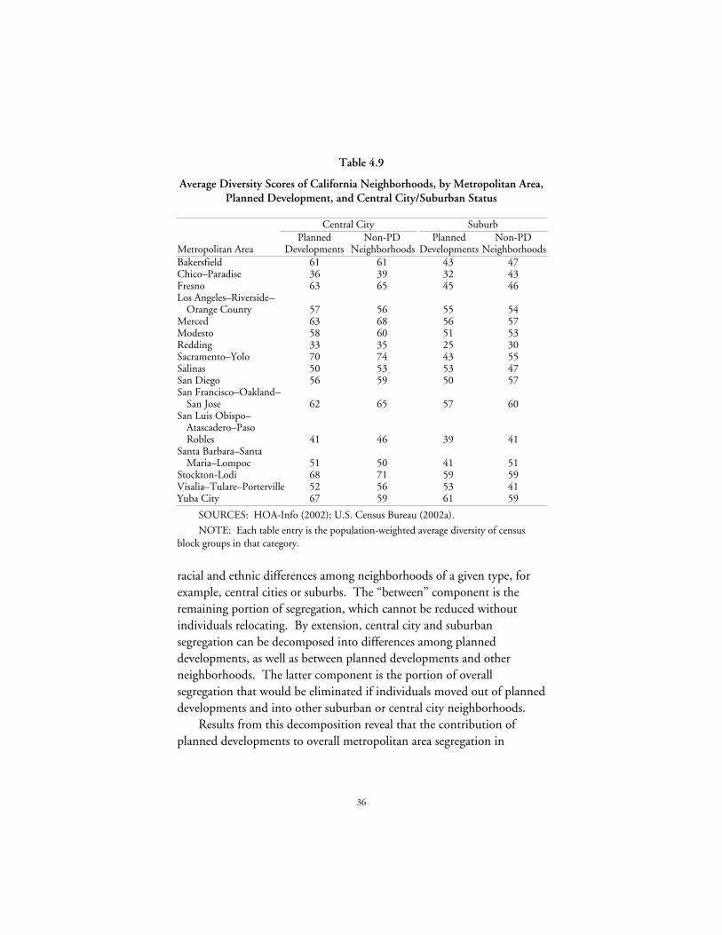
36

Table 4.9

Average Diversity Scores of California Neighborhoods, by Metropolitan Area,Planned Development, and Central City/Suburban Status

Central City Suburb

Metropolitan AreaPlanned

DevelopmentsNon-PD


DevelopmentsNon-PD

NeighborhoodsBakersfield 61 61 43 47Chico–Paradise 36 39 32 43Fresno 63 65 45 46Los Angeles–Riverside–

Orange County 57 56 55 54Merced 63 68 56 57Modesto 58 60 51 53Redding 33 35 25 30Sacramento–Yolo 70 74 43 55Salinas 50 53 53 47San Diego 56 59 50 57San Francisco–Oakland–

San Jose 62 65 57 60San Luis Obispo–

Atascadero–PasoRobles 41 46 39 41

Santa Barbara–SantaMaria–Lompoc 51 50 41 51

Stockton-Lodi 68 71 59 59Visalia–Tulare–Porterville 52 56 53 41Yuba City 67 59 61 59


NOTE: Each table entry is the population-weighted average diversity of censusblock groups in that category.

racial and ethnic differences among neighborhoods of a given type, forexample, central cities or suburbs. The “between” component is theremaining portion of segregation, which cannot be reduced withoutindividuals relocating. By extension, central city and suburbansegregation can be decomposed into differences among planneddevelopments, as well as between planned developments and otherneighborhoods. The latter component is the portion of overallsegregation that would be eliminated if individuals moved out of planneddevelopments and into other suburban or central city neighborhoods.

Results from this decomposition reveal that the contribution ofplanned developments to overall metropolitan area segregation in

37

California is actually quite small (Table 4.10). In suburbs, differences inthe racial and ethnic composition between planned developments andother neighborhoods explain only 2 percent of overall segregation. Incentral cities, the share attributable to planned developments is evensmaller at 1 percent. (Appendix B includes decompositions of segregationindices by metropolitan area.)

This finding is perhaps unsurprising because of the small proportionof the population currently living in planned developments. Recall thatdecompositions of the entropy measure of segregation reflect the relativepopulation shares in each geographic component. Although planneddevelopments represent more than 40 percent of new single-familyhomes, they include less than 20 percent of the existing stock of thesehomes and 12 percent of total units (HOA-Info, 2002; U.S. CensusBureau, 2002a). In light of racial and ethnic differences betweenplanned developments and other neighborhoods presented in thischapter, it is conceivable that as these communities proliferate, theycould exert a greater effect on residential segregation over time.

Table 4.10

Decomposition of Statewide Metropolitan Racial Segregation

Component % ShareBetween central cities and suburbs 2Central cities 43

Between planned developments and other neighborhoods 1Within planned developments 4Within other neighborhoods 37

Suburbs 56Between planned developments and other neighborhoods 2Within planned developments 9Within other neighborhoods 44


NOTE: Numbers may not sum to 100 because of rounding.

39

5. Voting Behavior

This chapter investigates the voting behavior of Californians living inplanned developments. It begins with a look at linkages between so-called “private governments” and political participation, as measured byvoter turnout, registration, and party affiliation. It then considersdifferences between planned developments and other neighborhoods in“yes” votes on statewide ballot propositions. Finally, it examines howrobust these differences are even after controlling for other factors thatmight influence voting behavior.

Many social commentators have expressed concerns about residentsof common interest developments opting out of the public sphere.Perhaps most famously, Robert Reich has referred to the growth of CIDsas the “secession of the successful.” Similarly, Charles Murray (1991, p.26) has expressed concern about the democratizing potential of CIDs toallow “10 or 20 percent of the population… to bypass social institutionsit doesn’t like in ways that only the top fraction of 1 percent used to beable to do.” One argument is that the homogeneity of thesecommunities reduces the incentives, or controversies, that draw citizensinto civic affairs (e.g., Putnam, 2000; Oliver, 2001).1 Alternatively, ifplanned developments are substitutes for traditional local government,then residents of these developments may perceive less benefit to takingpart in elections and other aspects of public life (e.g., Blakely and Snyder,1997).

These concerns have taken on added meaning in light of recentevidence for declining “social capital” in the United States, asdocumented in Robert Putnam’s Bowling Alone. Analogous to physicalor human capital, social capital refers to the stock of social norms, trust,and civic engagement that enhances both individual productivity and____________

1See Alesina and La Ferrara (2000) for an opposing view, i.e., that heterogeneitydepresses participation in voluntary associations.

40

aggregate welfare. Indicators include voter turnout and other forms ofpolitical participation, membership in voluntary associations, and surveysregarding trust in government. Turnout in U.S. presidential electionshas fallen from roughly 63 percent of the voting age population in 1960to 51 percent in 2000 (U.S. Federal Elections Commission, 2000). InCalifornia, voter turnout has fallen from roughly 50 percent innonpresidential statewide elections during the 1970s to 36 percent inNovember 2002 (California Secretary of State, 2002). Moreover, as inthe rest of the nation, few Californians are involved in political parties,elections, or campaigns (e.g., Baldassare, 2000, p. 34; Verba, Scholzman,and Brady, 1995). These trends could have lasting consequences to theextent that government policies tend to reflect the preferences of thosewho participate in public life.

There are several reasons, however, to believe that residents ofplanned developments will be more rather than less politically active. Asseen in the previous chapter, residents of these communities tend to beolder, better educated, and more affluent—factors that are all associatedwith higher rates of voter turnout (e.g., Rosenstone and Hansen, 1993).Beyond these factors, homeowners in general are more likely to take partin elections and other forms of civic participation because of an interestin preserving neighborhood quality and property values (DiPasquale andGlaeser, 1999).2 According to one gated community residentinterviewed by Blakely and Snyder (1997, p. 72), for instance,

The reason for the activism in Rancho Mirage and Indian Wells is the residentsare rich and used to having their voices heard, and they are retired and havetime. Also, the gated community has a stronger investment in expressing theirneeds because they identify with that community. Neighborhoods would havedrawn that kind of allegiance in the past. There has been a sense of belongingand of shared destiny between an individual and where they live throughouthistory which has been lost. The gated community replaces that. I’mwondering if they aren’t a market response to that desire for belonging. . . .The gate and the homogeneity reinforces a feeling of shared destiny and[shared interest in] property values .

____________ 2Homeowners may also self-select into these communities because of an interest in

preserving property values, for example, through more stringent land use and otherregulation (Helsley and Strange, 2000). See Appendix C for a discussion of the selectionissue.

41

This motivation further suggests that members of planneddevelopments may vote differently from other Californians. Inparticular, in keeping with the “double taxation” issue discussed at theend of Chapter 2, they may favor public spending that complementsprivate expenditures (e.g., police protection) while opposing that which isduplicative or redistributive (e.g., infrastructure and welfare).

This chapter tests the above hypotheses using voting and registrationinformation from the 2000 statewide general election.3 Results indicatethat members of planned developments do not exhibit significantlydifferent voting behavior once relevant demographic characteristics aretaken into account. These findings undermine the popular view that so-called “private governments” crowd out political participation orinfluence the direction of voting behavior on individual ballotpropositions, at least in statewide general elections.

Voter Turnout, Registration, and Party AffiliationPlanned developments exhibit higher rates of voter turnout and

registration than other California neighborhoods (Table 5.1).Differences in turnout between planned developments and otherneighborhoods are 6 percentage points, on average, whereas those invoter registration are even higher at 8 percentage points. Planneddevelopments are more politically conservative than otherneighborhoods, with higher Republican Party registration (by about 9percentage points) and lower Democratic Party affiliation (by roughly 8percentage points). (These differences are statistically significant at the 1percent level).

Voting on Statewide Ballot PropositionsDifferences in political ideology are apparent not only in the party

affiliation of planned development residents but also in their patterns ofvoting on statewide ballot propositions (Table 5.2). In the 2000statewide general election, residents of planned developments were morelikely to support measures related to privatization, such as school____________

3These data were matched to census levels of geography by the Statewide Databaseat UC Berkeley’s Institute of Governmental Studies. See Statewide Database (2002).

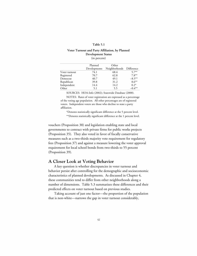
42

Table 5.1

Voter Turnout and Party Affiliation, by PlannedDevelopment Status

(in percent)

PlannedDevelopments

OtherNeighborhoods Difference

Voter turnout 74.1 68.4 5.7**Registered 70.7 62.8 7.8**Democrat 40.7 49.1 –8.5**Republican 39.8 31.2 8.6**Independent 14.4 14.2 0.2*Other 5.1 5.5 –0.4**

SOURCES: HOA-Info (2002); Statewide Database (2000).

NOTES: Rates of voter registration are expressed as a percentageof the voting age population. All other percentages are of registeredvoters. Independent voters are those who decline to state a partyaffiliation.



vouchers (Proposition 38) and legislation enabling state and localgovernments to contract with private firms for public works projects(Proposition 35). They also voted in favor of fiscally conservativemeasures such as a two-thirds majority vote requirement for regulatoryfees (Proposition 37) and against a measure lowering the voter approvalrequirement for local school bonds from two-thirds to 55 percent(Proposition 39).

A Closer Look at Voting BehaviorA key question is whether discrepancies in voter turnout and

behavior persist after controlling for the demographic and socioeconomiccharacteristics of planned developments. As discussed in Chapter 4,these communities tend to differ from other neighborhoods along anumber of dimensions. Table 5.3 summarizes these differences and theirpredicted effects on voter turnout based on previous studies.

Taking account of just one factor—the proportion of the populationthat is non-white—narrows the gap in voter turnout considerably,

43

Table 5.2

Approval Rates for Statewide Ballot Propositions, by Planned DevelopmentStatus (in percent)

Prop.No. Purpose

PlannedDevelopments


32 $500,000,000 bond issue for farm andhome aid to California veterans 66 69 –3**

33 Allows California legislature toparticipate in the Public Employees'Retirement System 37 41 –3**

34 Limits individual campaigncontributions; establishes voluntaryspending limits; expands publicdisclosure requirements 60 61 –1**

35 Provides that state and localgovernments may contract withprivate entities for engineering andarchitectural services 58 53 5**

36 Requires probation and treatment forconviction of possession, use,transportation, or being underinfluence of controlled substances 60 62 –3**

37 Requires two-thirds vote of statelegislature, or either majority or two-thirds of local electorate, to imposeany activity fees to monitor, study, ormitigate effects of that activity 49 47 2**

38 Authorizes state-funded schoolvouchers of $4,000 per pupil per yearfor private and religious schools 31 28 3**

39 Authorizes bonds for repair,construction, or replacement ofschool facilities, classrooms, ifapproved by a 55 percent local vote 52 56 –5**


NOTE: Differences may not be precise because of rounding.


although differences remain statistically significant at the 1 percent level(Table 5.4).

More strikingly, the gap in voter registration between planneddevelopments and other neighborhoods is all but eliminated aftercontrolling for the proportion of the population that is non-white (Table5.5).

44

Table 5.3

Summary of Demographic and Socioeconomic Differences BetweenPlanned Developments and Other Neighborhoods and

Predicted Effects on Voter Turnout (in percent)

Characteristic

PlannedDevelopments


Predicted Effecton Turnout

White 64 47 17** IncreasesIncome above $75,000 37 26 11** IncreasesWith college degree 21 15 6** IncreasesAges 40 to 64 33 29 4** IncreasesAge 65 and up 14 11 2** IncreasesHomeowner 66 57 9** IncreasesMoved in last 5 years 49 48 1** Decreases




Table 5.4

Voter Turnout, by Planned Development Status andRacial and Ethnic Diversity (in percent)

PercentageNon-White

PlannedDevelopments


0–25 79 77 2**25–50 74 72 2**50–75 69 66 2**75–100 63 60 3**



**Denotes statistically significant difference at the 1 percentlevel.

Regression analysis enables us to control for many demographic andsocioeconomic characteristics simultaneously, thereby parsing out theeffect of planned developments alone, all else being equal. Figure 5.1summarizes the estimated effect of planned developments on votingbehavior, holding constant other neighborhood features such as agestructure, levels of educational attainment, income mix, racial and ethniccomposition, homeownership, and urban location.4

____________ 4Appendix C includes detailed regression results and a discussion of modeling issues.

45

Table 5.5

Voter Registration, by Planned Development Status andRacial and Ethnic Diversity (in percent)

PercentageNon-White

PlannedDevelopments


0–25 81 80 125–50 72 71 150–75 59 59 075–100 46 47 –1*

SOURCES: HOA-Info (2002); Statewide Database(2000).


*Denotes statistically significant difference at the 5percent level.

Raw difference in means Controlled difference in means


–10

–8

–6

–4

–2

0

2

4

6

8

10

Per

cent

age

poin

ts

Voter turnout Percentregistered

PercentRepublican

PercentDemocrat

PercentIndependent

Figure 5.1—Estimated Effects of Planned Developments on Voter Turnout,Registration, and Party Affiliation

46

Differences in voter turnout, registration, and party affiliationbetween planned development and other neighborhoods are reducedsubstantially after controlling for these influences. Results from theregression model indicate that planned developments have rates of voterturnout that are higher by two-thirds of 1 percentage point; this is incontrast to the 6 percentage points detected in the uncontrolleddifference. More dramatically, differences in voter registration ratesswitch from a positive 8 percentage points to a negative 0.77 percentagepoints. In other words, planned developments exhibit slightly lower ratesof voter registration than we would expect given residents’ socioeconomicstatus.

Differences in party affiliation, although muted, are still apparent.Residents of planned developments are more likely to register with theRepublican Party, for an average difference of approximately 2percentage points, with a nearly offsetting reduction in Democratic Partyaffiliation.

Regressions seeking to explain voting on statewide ballotpropositions hold constant Republican Party registration in addition tothe demographic and socioeconomic neighborhood attributes describedabove. Again, the gap in voting behavior between planned developmentsand other areas narrows considerably (Figure 5.2). Differences inpercentage voting in favor of “conservative” measures—such as schoolvouchers (Proposition 38), state and local government contracting outfor public works projects (Proposition 35), and a two-thirds voterequirement for fees (Proposition 37)—drop to 1 percentage point orless. In contrast to the uncontrolled differences presented above, planneddevelopments are associated with slightly higher approval rates formeasures to lower the vote requirement for local school bonds(Proposition 39) and to issue a bond for veterans (Proposition 32).

In general, these differences, although statistically significant, arequite small. Taken together, they suggest that planned developments donot strongly affect either political participation or patterns of votingbehavior in statewide general elections. Residents of planneddevelopments vote similarly to other Californians of comparable age,income, education, race, and ethnicity.

47

Raw difference in means Controlled difference in means


–6

–4

–2

0

2

4

6

Per

cent

age

poin

ts

Proposition 32 Proposition 35 Proposition 37 Proposition 38 Proposition 39

Figure 5.2—Estimated Effects of Planned Developments on Votes forStatewide Ballot Propositions

49

6. Conclusions

Common interest developments are a dominant source of newhousing in California. This report is one of the first empirical analyses ofthese communities. It presents a comprehensive overview of commoninterest developments in general, including their origins, institutionalfeatures, and powers and responsibilities and compares them totraditional local government. It also surveys the features of commoninterest development housing in California, documenting trends in thelocation, size, and financial resources of these communities.

The report focuses on one particular type of common interestdevelopment, the planned development. This is the fastest-growing andmost prevalent CID as well as the most direct form of potentialcompetition with traditional local government. The study relies on avariety of data sources to describe these communities and discern theirpotential consequences for residential segregation and civic engagement.

Results indicate that concerns regarding negative social consequencesof planned developments are, for the most part, unwarranted. Planneddevelopments are less diverse than other neighborhoods, yet theircontribution to area segregation is minor. Similarly, planneddevelopments do not exhibit differences in political participation orvoting behavior once relevant demographic and socioeconomic factorsare taken into consideration.

There are several important caveats to bear in mind, however. Asrecent trends in the growth of the population and planned developmentscontinue, it is conceivable that the effects of these communities onresidential segregation may become more pronounced. Althoughplanned developments currently represent only 12 percent of all housingunits, they constitute roughly 30 percent of new housing starts and over40 percent of new single-family home sales (HOA-Info, 2002; U.S.Census Bureau, 1994, 1995, 1996, 1998, 1999, 2002b; ConstructionIndustry Research Board, 2000).

50

Local authorities may wish to consider such potential costs beforeencouraging this form of development to offset the costs of additionalpublic services and infrastructure. Nevertheless, eliminating planneddevelopments altogether would not necessarily reduce segregation evenby the modest amounts suggested in Chapter 4. These developmentsare but one way that individuals can sort themselves based on desires foreither enhanced services or racial and economic homogeneity.

In addition, voting behavior in statewide general elections is only oneform of political participation, albeit one that is more tractable forempirical analysis. Other important indicators of civic engagementinclude joining in voluntary associations, contacting elected officials, andattending public hearings or meetings. An important area for futureresearch is the level of involvement within common interestdevelopments themselves through boards of directors and committees.Only this information will illuminate the total effect of planneddevelopments on participation in public life.

Finally, a consistent and important finding throughout the report isthe considerable heterogeneity among common interest developments ingeneral and planned developments specifically. This finding in particularmilitates against any “one-size-fits-all” policy solution.

51

Appendix A

Data and Methods

This appendix describes the procedure used to match locations ofplanned developments to U.S. Census Bureau geography. It alsoexplores the potential consequences of the limitations of this procedurefor results presented in the report. In some cases, it presents resultsseparately based on alternative sample definitions.

Planned development addresses in the HOA-Info database weregeocoded—matched to latitude and longitude coordinates usinggeographic information systems (GIS). Matching was successful forabout 8,100, or 94 percent, of the approximately 8,600 planneddevelopments for which address information was reported.1 Thesecoordinates were then used to link each property to census levels ofgeography (e.g., blocks, block groups, and tracts) and politicaljurisdictions (e.g., cities, counties) (Figure A.1).

Geographic matches were based on the reported street address of thehomeowner association president. Properties reporting only a manageraddress were excluded from the sample, as were any properties reportinganomalous addresses that could not be reliably distinguished from off-sitemanagement companies.2 This procedure yielded roughly 6,200, or 66percent, of all planned developments that existed in California as ofDecember 2002.____________

1Of the 9,318 planned developments in the dataset, address information wasmissing for 667 observations. Searches of homeowner association websites and directoriesas well as public tax assessment, deed transfer, and mortgage records yielded locations forseveral missing PDs. These developments were statistically indistinguishable fromplanned developments that did report address information on all observable dimensionsexcept size (i.e., number of units and acreage), most likely reflecting the procedure used tolocate missing addresses rather than systematic reasons for reporting or not reporting tothe California Department of Real Estate or Secretary of State.

2These include multiple records with identical addresses except for homeownerassociations that are affiliated with one another (e.g., separate building phases of the samedevelopment). Unique observations in areas that were zoned predominantly for commercialor industrial use according to county assessor data were also purged from the analysis.

52

Figure A.1—Example of Geocoding Procedure

This sample differs somewhat from the population of planneddevelopments as a whole. Notably, they are significantly smaller andolder than other planned developments (Table A.1). These differencesmay reflect the tendency for larger and newer developments to report off-site management companies as their primary address; these would beexcluded from the sample. Efforts to obtain address information fromlarge property management companies were unsuccessful because ofconfidentiality concerns.

Table A.2 shows that excluding these developments from the study isunlikely to bias results toward zero because they constitute a smallproportion of total housing. In other words, they do not constitute alarge enough share of all units to contaminate the “control group.”

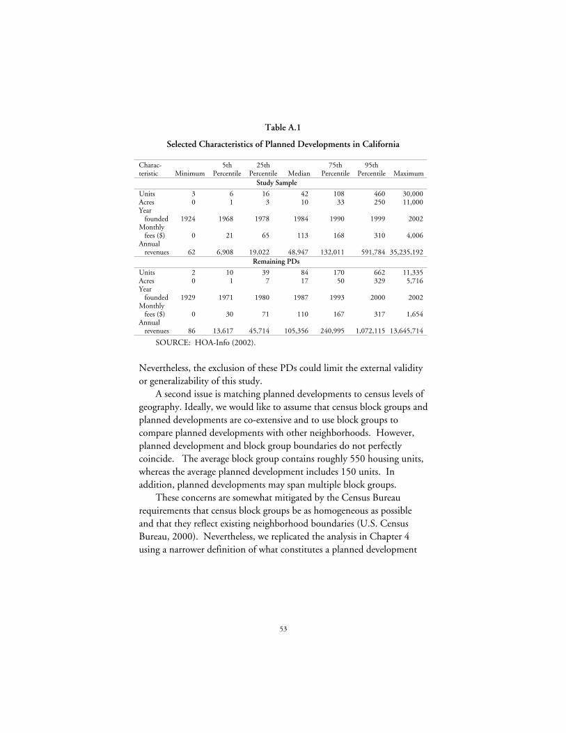
53

Table A.1

Selected Characteristics of Planned Developments in California

Charac-teristic Minimum

5thPercentile

25thPercentile Median

75thPercentile

95thPercentile Maximum

Study Sample

Units 3 6 16 42 108 460 30,000Acres 0 1 3 10 33 250 11,000Year

founded 1924 1968 1978 1984 1990 1999 2002Monthly

fees ($) 0 21 65 113 168 310 4,006Annual

revenues 62 6,908 19,022 48,947 132,011 591,784 35,235,192Remaining PDs

Units 2 10 39 84 170 662 11,335Acres 0 1 7 17 50 329 5,716Year

founded 1929 1971 1980 1987 1993 2000 2002Monthly

fees ($) 0 30 71 110 167 317 1,654Annual

revenues 86 13,617 45,714 105,356 240,995 1,072,115 13,645,714


Nevertheless, the exclusion of these PDs could limit the external validityor generalizability of this study.

A second issue is matching planned developments to census levels ofgeography. Ideally, we would like to assume that census block groups andplanned developments are co-extensive and to use block groups tocompare planned developments with other neighborhoods. However,planned development and block group boundaries do not perfectlycoincide. The average block group contains roughly 550 housing units,whereas the average planned development includes 150 units. Inaddition, planned developments may span multiple block groups.

These concerns are somewhat mitigated by the Census Bureaurequirements that census block groups be as homogeneous as possibleand that they reflect existing neighborhood boundaries (U.S. CensusBureau, 2000). Nevertheless, we replicated the analysis in Chapter 4using a narrower definition of what constitutes a planned development

54

Table A.2

Regional Distribution of Planned Development Units, by Sample Definition

Region Study Sample Remaining PDsTotal Housing

UnitsBay Area 159,501 106,307 2,552,402

6 4Central Coast 40,444 5,388 492,256

8 1North Coast and Mountains 57,946 16,971 488,006

12 3Inland Empire 111,695 93,894 1,186,043

9 8Sacramento Metro 73,926 35,183 714,981

10 5San Diego 88,866 98,134 1,084,040

8 9San Joaquin Valley 79,259 31,167 1,107,260

7 3Sierras 21,587 3,493 97,456

22 4South Coast 216,719 245,324 4,492,105

5 5Total 849,943 635,861 12,214,549

7 5


NOTE: The numbers in the second row for each region are percentages.

block group.3 Findings were not substantially different in sign or inmagnitude. Results are available from the author upon request.____________

3Specifically, to avoid mistakenly characterizing block groups as planneddevelopments, we restricted the sample to block groups where PDs constituted a majority(60 percent) of the housing stock. Many of these block groups included more planneddevelopment units than total housing units, suggesting a PD that spans multiple blockgroups. To address this second type of error, we coded all block groups within a censustract as planned developments if the “spillover” from the initial PD constituted more than70 percent of all housing units in the tract.

55

Appendix B

Measuring Diversity and Segregation

This appendix reviews the entropy measures of diversity andsegregation. It also presents results for the decomposition of segregationmeasures by metropolitan area (Table B.1).

The entropy index of diversity for a city or metropolitan area is

E Q

Qrrr

n=

⎛⎝⎜

⎞⎠⎟

∑=

log1

1(B.1)

where Qr is the proportion of the total population in group r, and n isthe number of groups. Analogously, for a neighborhood the index isdefined as

E q

qi ririr

n=

⎛⎝⎜

⎞⎠⎟

∑=

log1

1(B.2)

where qri is the proportion of individuals belonging to racial or ethnicgroup r in neighborhood i.

Conceptually, the index expresses the level of uncertainty as to theracial or ethnic identity of any individual selected at random from thearea as a whole. It reaches its maximum of log(n) when all groups areequally represented in the population and its minimum of 0 when thereis only one group present. Index values can be normalized to rangebetween 0 and 100 by using the number of groups, n, as the base of thelogarithm and multiplying by 100.

The entropy index of segregation relates the diversity of a city ormetropolitan area as a whole to the population-weighted average diversityof its constituent neighborhoods:

H

t T E E

E

i ii

k

=−∑

=[ / ( )]

1 (B.3)

Tab

le B

.1

Dec

ompo

siti

on o

f Seg

rega

tion

, by

Pla

nned

Dev

elop

men

t an

d C

entr

al C

ity/

Subu

rban

Sta

tus

Bet

wee

nW

ithi

n C

entr

al C

itie

sW

ithi

n Su

burb

sC

entr

alC

itie

s an

dSu

burb

s

Tot

alC

entr

alC

itie

s

Bet

wee

nPD

s an

dN

on-P

Ds

Wit

hin

PDs

Wit

hin

Non

-PD

sT

otal

Subu

rbs

Bet

wee

nPD

s an

dN

on-P

Ds

Wit

hin

PDs

Wit

hin

Non

-PD

sT

otal

Met

ropo

litan

Are

a(1

)(2

)(3

)(4

)(5

)(6

)(7

)(8

)(9

)(1

0)B

aker

sfie

ld0.

846.

140.

580.

774.

7917

.66

1.54

1.32

14.8

24.4

325

23

1972

65

6010

0C

hico

–Par

adis

e0.

154.

590.

060.

793.

748.

460.

390.

507.

5713

.19

135

06

2864

34

5710

0Fr

esno

1.67

10.3

90.

721.

088.

5911

.86

0.8

0.8

10.2

623

.94

743

35

3650

33

4310

0Lo

s A

ngel

es–R

iver

side

–O

rang

e C

ount

y0.

4311

.24

0.42

0.6

10.2

218

.59

0.45

2.57

15.5

730

.25

137

12

3461

18

5110

0M

erce

d0.

975.

110.

340.

114.

669.

470.

140.

259.

0815

.54

633

21

3061

12

5810

0M

odes

to0.

867.

230.

320.

686.

235.

20.

240.

194.

7713

.36

542

547

392

136

100

Red

ding

0.98

2.58

0.06

0.65

1.87

3.48

0.12

0.14

3.22

7.03

1437

19

2750

22

4610

0Sa

cram

ento

–Yol

o2.

95.

450.

180.

734.

549.

140.

591.

576.

9817

.517

311

426

523

940

100

Salin

as1.

259.

930.

063.

86.

0717

.18

0.92

4.62

11.6

428

.36

435

013

2161

316

4110

0Sa

n D

iego

0.93

13.6

80.

551.

4611

.67

8.42

0.59

1.6

6.23

23.0

24

592

651

373

727

100

56

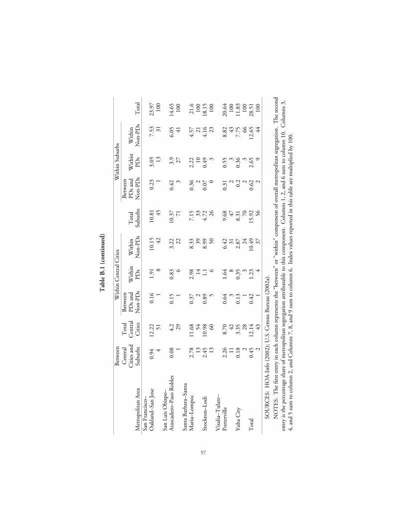
Tab

le B

.1 (

cont

inue

d)

Bet

wee

nW

ithi

n C

entr

al C

itie

sW

ithi

n Su

burb

s

Met

ropo

litan

Are

a

Cen

tral

Cit

ies

and

Subu

rbs

Tot

alC

entr

alC

itie

s

Bet

wee

nPD

s an

dN

on-P

Ds

Wit

hin

PDs

Wit

hin

Non

-PD

sT

otal

Subu

rbs

Bet

wee

nPD

s an

dN

on-P

Ds

Wit

hin

PDs

Wit

hin

Non

-PD

sT

otal

San

Fran

cisc

o–O

akla

nd–S

an J

ose

0.94

12.2

20.

161.

9110

.15

10.8

10.

233.

057.

5323

.97

451

18

4245

113

3110

0Sa

n Lu

is O

bisp

o–A

tasc

ader

o–Pa

so R

oble

s0.

084.

20.

150.

833.

2210

.37

0.42

3.9

6.05

14.6

51

291

622

713

2741

100

Sant

a B

arba

ra–S

anta

Mar

ia–L

ompo

c2.

7811

.68

0.37

2.98

8.33

7.15

0.36

2.22

4.57

21.6

1354

214

3933

210

2110

0St

ockt

on–L

odi

2.45

10.9

80.

891.

18.

994.

720.

070.

494.

1618

.15

1360

56

5026

03

2310

0V

isal

ia–T

ular

e–Po

rter

ville

2.26

8.70

0.64

1.64

6.42

9.68

0.31

0.55

8.82

20.6

411

423

831

472

343

100

Yub

a C

ity

0.18

3.35

0.13

0.35

2.87

8.31

0.2

0.36

7.75

11.8

32

281

324

702

366

100

Tot

al0.

4512

.14

0.42

1.23

10.4

915

.92

0.62

2.65

12.6

528

.51

243

14

3756

29

4410

0

SOU

RC

ES:

HO

A-I

nfo

(200

2); U

.S. C

ensu

s B

urea

u (2

002a

).

NO

TE

S: T

he fi

rst e

ntry

in e

ach

colu

mn

repr

esen

ts th

e “b

etw

een”

or

“wit

hin”

com

pone

nt o

f ove

rall

met

ropo

litan

seg

rega

tion

. T

he s

econ

den

try

is th

e pe

rcen

tage

sha

re o

f met

ropo

litan

seg

rega

tion

att

ribu

tabl

e to

this

com

pone

nt.

Col

umns

1, 2

, and

6 s

um to

col

umn

10.

Col

umns

3,

4, a

nd 5

sum

to c

olum

n 2,

and

Col

umns

7, 8

, and

9 s

um to

col

umn

6. I

ndex

val

ues

repo

rted

in th

is ta

ble

are

mul

tipl

ied

by 1

00.

57

58

where T and ti are the respective area and subunit populations and k is thenumber of subunits. Since the entropy of an area as a whole (i.e., E ) cannever be less than the average entropy of its parts (i.e., ( / ) )t T Eii

ki=∑ 1 ),

the segregation index necessarily ranges between 0 and 1. At 0, the racialcomposition of each subunit is identical to that of the area as a whole,whereas at 1 each subunit contains only one group.

An attractive feature of the entropy index of segregation is that itmay be decomposed into segregation between and within groups. Thegeneral formula for any decomposition is

H

T

T

E

EH

p

p P

pp=

⎛

⎝⎜⎞

⎠⎟∑

⎛

⎝⎜⎞

⎠⎟∈(B.4)

where p represents racial or geographic components of the decomposition(Reardon et al., 2000, p. 354). For instance, the segregation of ametropolitan area comprising central city and suburban block groups canbe written as

H H

TT

EE

HTT

EE

Hc sc c

cs s

s= + ⎛⎝⎜

⎞⎠⎟⎛⎝⎜

⎞⎠⎟

+ ⎛⎝⎜

⎞⎠⎟⎛⎝⎜

⎞⎠⎟, (B.5)

where Tc and Ts, Ec and Es, and Hc and Hs are, respectively, the totalpopulations, entropy measures of diversity, and entropy measures ofsegregation for city and suburban block groups (Reardon et al., 2000, p.355). The first term, Hc,s, indicates the portion of overall segregationattributable to differences between the central city and the suburbs.That is

H

T E T ETEc s

c c s s, .= − +⎛

⎝⎜⎞⎠⎟

1 (B.6)

The second and third terms represent portions of segregationattributable to differences among central city and suburban subunits.These latter terms can be further decomposed into “between” and“within” components with respect to planned development status.Specifically, each “within” term in Equation (B.5) above includes

59

H

TT

EE

HT

TE

EHPD non PD

PD PDPD

non PD non PDnon PD, −

− −−+ ⎛

⎝⎜⎞⎠⎟⎛⎝⎜

⎞⎠⎟

+ ⎛⎝⎜

⎞⎠⎟⎛⎝⎜

⎞⎠⎟

(B.7)

where the first term is segregation between planned developments andother block groups defined analogously to Equation (B.6), the secondterm represents the share of segregation among planned developments,and the third term represents the share of segregation among non-PDblock groups.

61

Appendix C

Technical Considerations andRegression Results

A methodological complication in any study of neighborhood effectson political participation is the potential endogeneity of residentialchoice. That is, individuals may choose to live in a planned developmentbecause of observable or unobservable factors that are also related tovoting behavior. As a result, apparent relationships between planneddevelopments and voter turnout may be spurious. This selection bias canwork in either direction. For example, individuals may sort into aplanned development based on a taste for involvement in both publicand private government. Alternatively, they may move into a PD to optout of the public sphere without sacrificing collective goods and services.In either case, estimates of the effect of living in a planned developmentwill be both biased and inconsistent.

Gordon (2003) explores this possibility using several specifications tocontrol for potential selection bias. Methods include least squaresregression with block-group fixed effects, a Heckman selection correctionmodel, and a propensity-score approach. Results from these models arenot substantially different from the least squares regression withdemographic covariates presented in this report.1

The remainder of this appendix includes detailed results from themultivariate analysis underlying the charts in Chapter 5.____________

1Gordon (2003) also includes results of regressions based on a more restrictedsample definition as in Appendix A.

62

Table C.1

Estimated Effects of Planned Developments on Voter Turnout, 2000

Differencein Means

OrdinaryLeast Squares

Planned development 5.700 0.661= 1 if > 1 PD (0.166)** (0.107)**= 0 otherwise

PercentageAges 40–64 0.093

(0.012)**Age 65 and older 0.173

(0.007)**Non–Hispanic black –0.118

(0.004)**Hispanic –0.053

(0.004)**Non–Hispanic Asian –0.123

(0.003)**With less than high school –0.160

(0.014)**High school diploma –0.049

(0.016)**With some college 0.023

(0.010)*With college degree 0.086

(0.011)**Homeowner 0.068

(0.004)**Moved in last 5 years –0.043

(0.005)**With income $50,000–$74,999 0.110

(0.009)**With income $75,000–$99,999 0.127

(0.010)**With income $100,000–$199,999 0.108

(0.009)**With income $200,000 and up 0.059

(0.009)**Urban (= 1 if in an urbanized area) –1.696

(0.226)**Constant 68.374 63.193

(0.079)** (0.855)**No. of observations 22,055 21,802R2 0.04 0.63

SOURCES: HOA-Info (2002); Statewide Database (2000).NOTES: Robust standard errors are in parentheses. Percentages are calculated over

individuals except for income, which is a proportion of all households.*Denotes statistically significant difference at the 5 percent level.**Denotes statistically significant difference at the 1 percent level.

63

Table C.2

Estimated Effects of Planned Developments on Percentage Registered, 2000

Differencein Means


Planned development 7.827 –0.765= 1 if > 1 PD (0.328)** (0.206)**= 0 otherwise


(0.022)**Age 65 and older 0.162

(0.014)**Non–Hispanic black 0.077

(0.007)**Hispanic –0.266





(0.019)**With college degree 0.379

(0.021)**Homeowner 0.150


(0.009)**With income $50,000–$74,999 0.010

(0.017)With income $75,000–$99,999 –0.006

(0.022)With income $100,000–$199,999 –0.009

(0.015)With income $200,000 and up 0.050

(0.018)**Urban (= 1 if in an urbanized area) 4.507

(0.440)**Constant 62.833 60.758




64

Table C.3

Estimated Effects of Planned Developments on Percentage RegisteredDemocrat, 2000

Differencein Means


Planned development –8.460 –1.807= 1 if > 1 PD (0.220)** (0.175)**= 0 otherwise


(0.014)**Age 65 and older 0.095


(0.004)**Hispanic 0.243

(0.006)**Non–Hispanic Asian 0.055


(0.016)High school diploma –0.061

(0.018)**With some college –0.272


(0.015)**Homeowner –0.065


(0.006)**With income $50,000–$74,999 –0.015

(0.011)With income $75,000–$99,999 –0.049

(0.013)**With income $100,000–$199,999 –0.100

(0.012)**With income $200,000 and up –0.143

(0.017)**Urban (= 1 if in an urbanized area) 5.243

(0.265)**Constant 49.116 46.224




65

Table C.4

Estimated Effects of Planned Developments on Percentage RegisteredRepublican, 2000

Differencein Means



PercentageAges 40–64 –0.126

(0.016)**Age 65 and older 0.044


(0.005)**Hispanic –0.185


(0.006)**With less than high school 0.026

(0.017)High school diploma 0.061


(0.015)**With college degree –0.153

(0.018)**Homeowner 0.152

(0.005)**Moved in last 5 years 0.134

(0.007)**With income $50,000–$74,999 0.007

(0.013)With income $75,000–$99,999 0.053

(0.014)**With income $100,000–$199,999 0.116



(0.333)**Constant 31.223 26.724




66

Table C.5

Estimated Effects of Planned Developments on Percentage RegisteredIndependent, 2000

Differencein Means


Planned development 0.211 –0.148= 1 if > 1 PD (0.079)** (0.061)*= 0 otherwise


(0.006)*Age 65 and older –0.070


(0.002)**Hispanic –0.023



(0.008)*High school diploma –0.002

(0.008)With some college –0.002

(0.006)With college degree 0.061

(0.007)**Homeowner –0.065


(0.003)**With income $50,000–$74,999 0.027

(0.004)**With income $75,000–$99,999 0.018

(0.005)**With income $100,000–$199,999 0.019


(0.006)Urban (= 1 if in an urbanized area) –0.077

(0.109)Constant 14.165 16.855




67

Table C.6

Estimated Effects of Planned Developments on “Yes” Votes forProposition 32, 2000

Differencein Means


Planned development –2.752 0.314= 1 if > 1 PD (0.096)** (0.066)**= 0 otherwise


(0.007)Age 65 and older 0.096


(0.003)**Hispanic 0.019



(0.010)High school diploma –0.007

(0.011)With some college –0.011

(0.007)With college degree –0.021

(0.007)**Homeowner –0.016


(0.003)With income $50,000–$74,999 –0.016

(0.005)**With income $75,000–$99,999 –0.027

(0.006)**With income $100,000–$199,999 –0.048


(0.007)Urban (= 1 if in an urbanized area) 0.678

(0.128)**Percent registered Republican –0.208

(0.003)**Constant 68.993 75.398

(0.048)** (0.567)**Observations 22,036 21,801R2 0.03 0.64


individuals except for income, which is a proportion of all households. Proposition 32 is a$500,000,000 bond issue for farm and home aid to California veterans.

*Denotes statistically significant difference at the 5 percent level.**Denotes statistically significant difference at the 1 percent level.

68

Table C.7


Differencein Means




(0.007)Age 65 and older –0.039


(0.003)**Hispanic –0.001

(0.003)Non–Hispanic Asian –0.025




(0.006)*With college degree 0.052

(0.007)**Homeowner –0.046


(0.003)**With income $50,000–$74,999 0.017

(0.005)**With income $75,000–$99,999 0.051

(0.007)**With income $100,000–$199,999 0.100



(0.140)**Percent registered Republican 0.287

(0.003)**Constant 52.509 42.972



individuals except for income, which is a proportion of all households. Proposition 35 allows stateand local governments to contract with private entities for engineering and architectural services.


69

Table C.8


Differencein Means


Planned development 2.331 0.167= 1 if > 1 PD (0.141)** (0.078)*= 0 otherwise


(0.008)Age 65 and up –0.021


(0.004)**Hispanic 0.097



(0.010)**High school diploma 0.135



(0.009)**Homeowner 0.009


(0.003)**With income $50,000–$74,999 –0.002

(0.007)With income $75,000–$99,999 0.003

(0.007)With income $100,000–$199,999 –0.022

(0.005)**With income $200,000 and up –0.066



(0.004)**Constant 46.991 21.736


SOURCES: HOA-Info (2002); Statewide Database (2000).NOTES: Robust standard errors are in parentheses. Percentages are calculated over individuals

except for income, which is a proportion of all households. Proposition 37 requires a vote of the statelegislature or local electorate to impose fees to monitor, study, or mitigate an activity.


70

Table C.9


Differencein Means


Planned development 2.662 0.112= 1 if > 1 PD (0.113)** (0.071)= 0 otherwise


(0.007)**Age 65 and up –0.033


(0.003)**Hispanic 0.024



(0.008)**High school diploma 0.087



(0.006)**Homeowner –0.018


(0.003)**With income $50,000–$74,999 0.003

(0.005)With income $75,000–$99,999 0.004

(0.005)With income $100,000–$199,999 –0.022


(0.007)**Urban (=1 if in an urbanized area) –1.84


(0.003)**Constant 28.282 13.645


SOURCES: HOA-Info (2002); Statewide Database (2000).NOTES: Robust standard errors are in parentheses. Percentages are calculated over individuals

except for income, which is a proportion of all households. Proposition 38 authorizes state-fundedschool vouchers of $4,000 per pupil per year for private and religious schools.


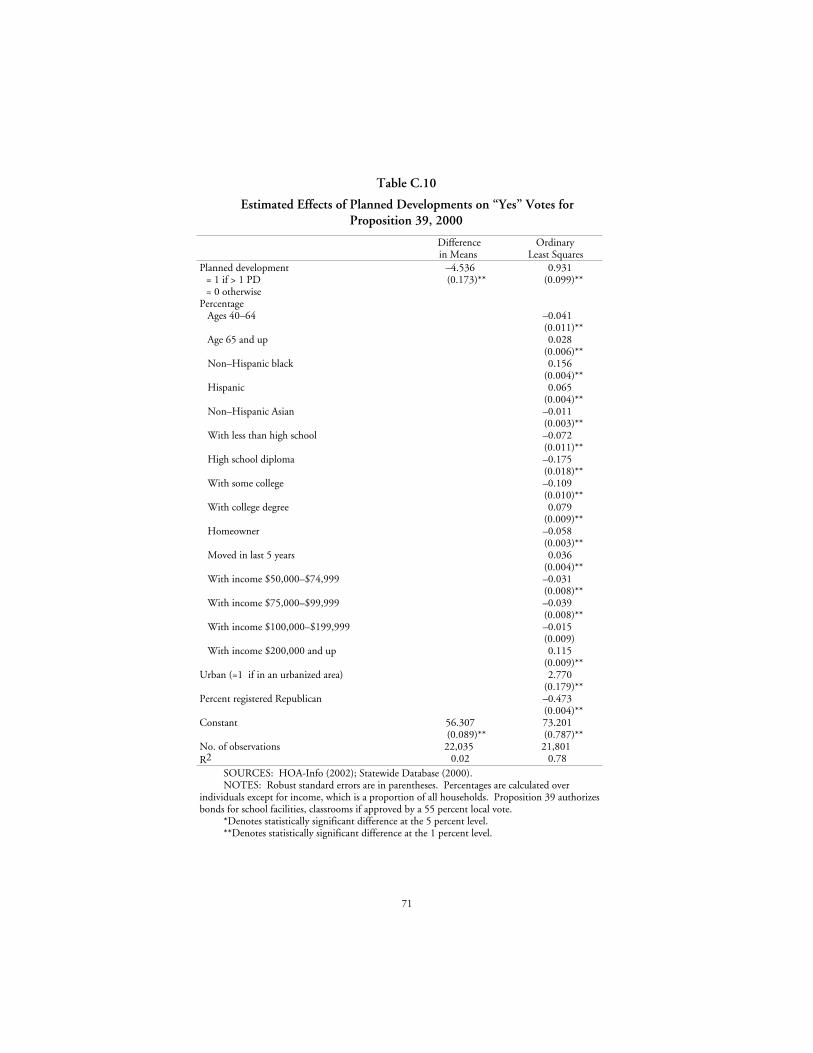
71

Table C.10


Differencein Means


Planned development –4.536 0.931= 1 if > 1 PD (0.173)** (0.099)**= 0 otherwise


(0.011)**Age 65 and up 0.028


(0.004)**Hispanic 0.065




(0.018)**With some college –0.109


(0.009)**Homeowner –0.058


(0.004)**With income $50,000–$74,999 –0.031

(0.008)**With income $75,000–$99,999 –0.039

(0.008)**With income $100,000–$199,999 –0.015

(0.009)With income $200,000 and up 0.115

(0.009)**Urban (=1 if in an urbanized area) 2.770

(0.179)**Percent registered Republican –0.473

(0.004)**Constant 56.307 73.201



individuals except for income, which is a proportion of all households. Proposition 39 authorizesbonds for school facilities, classrooms if approved by a 55 percent local vote.


73

References

Advisory Commission on Intergovernmental Relations, ResidentialCommunity Associations: Private Governments in the IntergovernmentalSystem? Washington, D.C., May 1989.

Alesina, Alberto, and Eliana La Ferrara, “Participation in HeterogeneousCommunities,” Quarterly Journal of Economics, Vol. 115, No. 3,August 2000, pp. 847–904.

Baldassare, Mark, California in the New Millennium, University ofCalifornia Press, Berkeley, California, and the Public Policy Instituteof California, San Francisco, California, 2000.

Barton, Stephen E., and Carol J. Silverman, “History and Structure ofthe Common Interest Community,” in Stephen E. Barton and CarolJ. Silverman, eds., Common Interest Communities: Private Governmentsand the Public Interest, Institute of Governmental Studies Press,Berkeley, California, 1994.

Barzel, Yoram, and Tim R. Sass, “The Allocation of Resources byVoting,” Quarterly Journal of Economics, Vol. 16, August, 1990, pp.745–771.

Black’s Law Dictionary, 5th ed., West Publishing Company, St. Paul,Minnesota, 1979.

Blakely, Edward J., and Mary Gail Snyder, Fortress America: GatedCommunities in the United States, Brookings Institution Press,Washington, D.C., 1997.

California Law Revision Commission, “Common Interest DevelopmentLaw: Scope of Project (Background Study),” Staff Memorandum2001-19, Palo Alto, California, January 22, 2001.

74

California Law Revision Commission, “Nonjudicial Dispute ResolutionUnder CID Law: Alternative Dispute Resolution (AdditionalInformation),” Second Supplement to Memorandum 2002-10, PaloAlto, California, 2002a.

California Law Revision Commission, “Alternative Dispute Resolutionin Common Interest Developments,” Tentative Recommendation,Palo Alto, California, 2002b.

California Secretary of State, Statement of Vote, 2002, available athttp://ss.ca.gov/elections/sov/2002_general/contents.htm.

Community Associations Institute, Data on U.S. Community Associations,2003, available at http://www.caionline.org/about/facts.cfm.

Construction Industry Research Board, Characteristics of New HomesSold: California and Selected Counties, 1982–1999, Burbank,California, 2000.

Devaney, John F., Tracking the American Dream: 50 Years of HousingHistory from the Census Bureau, 1940–1990, U.S. Department ofCommerce, Washington, D.C., 1994.

Dilger, Robert J., Neighborhood Politics: Residential CommunityAssociations in American Governance, New York University Press, NewYork, 1992.

DiPasquale, Denise, and Edward L. Glaeser, “Incentives and SocialCapital: Are Homeowners Better Citizens?” Journal for UrbanEconomics, Vol. 45, March 1999, pp. 354–384.

Egan, Timothy, “Many Seek Security in Private Communities,” NewYork Times, September 3, 1995, pp. A1, A22.

Ellickson, Robert C., “New Institutions for Old Neighborhoods,” DukeLaw Journal, Vol. 48, No. 1, 1998, pp. 75–110.

Foldvary, Fred, Public Goods and Private Communities: The MarketProvision of Social Services, Edward Elgar, Brookfield, Vermont, 1994.

75

Foldvary, Fred E., “Private Communities and Community Associations,”in David T. Beito, Peter Gordon, and Alex Tabarrok, eds., TheVoluntary City: Restoring Urban Life in Crisis Times, MichiganUniversity Press and The Independent Institute, Ann Arbor,Michigan, 2002.

French, Susan F., Scope of Laws Affecting Common Interest Developments,background study prepared for the California Law RevisionCommission, November 2000.

Gordon, Tracy M., “Crowd Out or Crowd In? The Effects of CommonInterest Developments on Political Participation in California,” TheAnnals of Regional Science, Vol. 37, No. 2, May 2003, pp. 203–233.

“Government by the Nice for the Nice,” The Economist, July 25, 1992,pp. A25–A27.

Helsley, Robert W., and William C. Strange, “Social Interactions and theInstitutions of Local Government,” American Economic Review, Vol.90, No. 5, 2000, pp. 1477–1490.

HOA-Info Information Services Division, HOA-Info, Oakland,California, 2002.

HOA-Info Information Services Division, California CommunityAssociation Statistics, Oakland, California, 2003.

Kennedy, David J., “Note: Residential Associations as State Actors:Regulating the Impact of Gated Communities on Nonmembers,” YaleLaw Journal, Vol. 105, December 1995, pp. 761–793.

Kress, Carl B., “Comment: Beyond Nahrstedt: Reviewing RestrictionsGoverning Life in a Property Owner Association,” UCLA Law Review,Vol. 42, 1995, pp. 837–883.

Lave-Johnston, Julia, and Kimberly Johnston-Dodds, Common InterestDevelopments: Housing at Risk? California Research Bureau,Sacramento, California, 2002.

Massey, Douglas S., and Nancy Denton, “The Dimensions of RacialSegregation,” Social Forces, Vol. 67, 1988, pp. 281–315.

76

McKenzie, Evan, Privatopia, Yale University Press, New Haven,Connecticut, 1994.

Murray, C., “The Shape of Things to Come,” National Review, Vol. 43,1991, pp. 26–31.

Nelson, Robert H., “Privatizing the Neighborhood: A Proposal toReplace Zoning with Private Collective Property Rights to ExistingNeighborhoods,” George Mason Law Review, Vol. 7, No. 4, Summer1999, pp. 827–880.

Oliver, Eric J., Democracy in Suburbia, Princeton University Press,Princeton, New Jersey, 2001.

Pack, Janet R., “BIDs, DIDs, SIDs, and SADs: Private Governments inUrban America,” Brookings Review, Fall 1992, pp. 18–21.

Putnam, Robert D., Bowling Alone: The Collapse and Revival of AmericanCommunity, Simon and Schuster, New York, 2000.

Reardon, Sean F., John T. Yun, and Tamela M. Eitle, “The ChangingStructure of School Segregation: Measurement and Evidence ofMultiracial Metropolitan-Area School Segregation, 1989–1995,”Demography, Vol. 37, No. 3, August 2000, pp. 351–364.

Reich, Robert B., “Secession of the Successful,” New York Times, January20, 1991, Section 6, p. 16.

Roland, Helen E., Residential Common Interest Developments: AnOverview, California Research Bureau, Sacramento, California, March1998.

Rosenstone, S. J., and J. M. Hansen, Mobilization, Participation, andDemocracy in America, Macmillan, New York, 1993.

Senate Housing and Community Development Committee, Hearing,“Common Interest Developments (CID’s): Incorporation andRegistration,” AB 643 Assembly Bill-Bill Analysis, July 1, 2002.

Statewide Database, Statewide Database, 2000, available at http://swdb.berkeley.edu/info/PDRDocument.txt.

77

Statewide Database, Documentation, 2002, available at http://swdb.berkeley.edu/data/data.html.

Theil, Henri, Statistical Decomposition Analysis, Amsterdam: North-Holland Publishing Co., 1972.

Tiebout, Charles M., “A Pure Theory of Local Public Expenditures,”Journal of Political Economy, Vol. 64, October 1956, pp. 416–424.

Tocqueville, Alexis de, Democracy in America, in J. P. Mayer, ed.,Anchor, Garden City, New Jersey, 1969 (1835), pp. 513–517.

Treese, Clifford J., Community Associations Factbook, CommunityAssociations Institute Research Foundation, Alexandria, Virginia,1999.

U.S. Census Bureau, Census of Housing, General Housing CharacteristicsCalifornia, U.S. Department of Commerce, Washington, D.C., 1970,1980, and 1990.

U.S. Census Bureau, Geographic Areas Reference Manual, U.S.Department of Commerce, Washington, D.C., 2000.

U.S. Census Bureau, Census 2000 Summary File 3—California,Washington, D.C., 2002a.

U.S. Census Bureau, Statistical Abstract, U.S. Department of Commerce,Washington, D.C., 1994, 1995, 1996, 1998, 1999, 2002b.

U.S. Federal Elections Commission, National Voter Turnout in FederalElections: 1960–1996, 2000, available at http://www.fec.gov/pages/htmlto5.htm.

Verba, S., K. L. Scholzman, and H. E. Brady, Voice and Equality: CivicVoluntarism in American Politics, Harvard University Press,Cambridge, Massachusetts, 1995.

Worley, William S., J. C. Nichols and the Shaping of a Kansas City:Innovation in Planned Residential Communities, University of MissouriPress, Columbia, Missouri, 1990.

79

About the Author

TRACY GORDON

Tracy Gordon is a research fellow at the Public Policy Institute ofCalifornia, where her research interests include state and local publicfinance and political economy. She has authored several journal articlesand conference papers on topics relating to local government, includingcommon interest developments and their effects on residentialsegregation and voting behavior, the local initiative process, and localproperty taxes. She holds a B.A. in human biology from StanfordUniversity and a Ph.D. in public policy with a concurrent M.A. ineconomics from the University of California, Berkeley.

81

Related PPIC Publications

Who Pays for Development Fees and Exactions?Marla Dresch and Steven M. Sheffrin

The Ties That Bind: Changing Demographics and Civic Engagement inCaliforniaS. Karthick Ramakrishnan and Mark Baldassare

“Who’s Your Neighbor? Residential Segregation and Diversity inCalifornia”California Counts: Population Trends and ProfilesVolume 4, Number 1, August 2002Juan Onésimo Sandoval, Hans P. Johnson, and Sonya M.Tafoya

“California’s Newest Neighborhoods”California Counts: Population Trends and ProfilesVolume 5, Number 1, August 2003Hans P. Johnson and Joseph M. Hayes

PPIC publications may be ordered by phone or from our website(800) 232-5343 [mainland U.S.]

(415) 291-4400 [Canada, Hawaii, overseas]www.ppic.org

Documents

Planned Developments in California: Private … Developments in California: Private Communities and Public Life ••• Tracy M. Gordon 2004