ARTICLE IN PRESS

Planetary and Space Science 57 (2009) 1671–1681

Contents lists available at ScienceDirect

Planetary and Space Science

0032-06

doi:10.1

� Corr

E-m

thomas

(L.N. Fle

(M. Roo

(B.J. Bur

(P.D. Ni

journal homepage: www.elsevier.com/locate/pss

Saturn’s north polar cyclone and hexagon at depth revealed by Cassini/VIMS

Kevin H. Baines a,�, Thomas W. Momary a, Leigh N. Fletcher b, Adam P. Showman c,Maarten Roos-Serote d, Robert H. Brown c, Bonnie J. Buratti e, Roger N. Clark f, Philip D. Nicholson g

a Jet Propulsion Laboratory, California Institute of Technology, MS 183-601, 4800 Oak Grove Drive, Pasadena, CA 91109, USAb Jet Propulsion Laboratory, California Institute of Technology, MS 169-237, 4800 Oak Grove Drive, Pasadena, CA 91109, USAc Lunar and Planetary Laboratory, University of Arizona, Tucson, AZ 85721, USAd Observatorio Astronomico de Lisboa, Tapada da Ajuda, 1349-018 Lisboa, Portugale Jet Propulsion Laboratory, California Institute of Technology, MS 183-501, 4800 Oak Grove Drive, Pasadena, CA 91109, USAf US Geological Survey, MS 964, Box 25046 Federal Center, Denver, CO 80225, USAg Cornell University, Astronomy Department, Space Sciences Building, Ithaca, NY 14853, USA

a r t i c l e i n f o

Article history:

Received 17 November 2008

Received in revised form

18 May 2009

Accepted 12 June 2009Available online 4 July 2009

Keywords:

Saturn

Cassini–Huygens

Visual-infrared mapping spectrometer

(VIMS)

Atmospheric dynamics

Polar cyclone

Saturn clouds

33/$ - see front matter & 2009 Elsevier Ltd. A

016/j.pss.2009.06.026

esponding author. Tel.: +1818 354 0481; fax:

ail addresses: kevin.baines@jpl.nasa.gov (K.H.

.w.momary@jpl.nasa.gov (T.W. Momary), Leig

tcher), showman@lpl.arizona.edu (A.P. Show

s-Serote), rhb@lpl.arizona.edu (R.H. Brown)

atti), rclark@usgs.gov (R.N. Clark), nicholso@a

cholson).

a b s t r a c t

A high-speed cyclonic vortex centered on the north pole of Saturn has been revealed by the visual-

infrared mapping spectrometer (VIMS) onboard the Cassini–Huygens Orbiter, thus showing that the

tropospheres of both poles of Saturn are occupied by cyclonic vortices with winds exceeding 135 m/s.

High-spatial-resolution (�200 km per pixel) images acquired predominantly under night-time

conditions during Saturn’s polar winter—using a thermal wavelength of 5.1mm to obtain time-lapsed

imagery of discrete, deep-seated (42.1-bar) cloud features viewed in silhouette against Saturn’s

internally generated thermal glow—show a classic cyclonic structure, with prograde winds exceeding

135 m/s at its maximum near 88.31 (planetocentric) latitude, and decreasing to o30 m/s at 89.71 near

the vortex center ando20 m/s at 80.51. High-speed winds, exceeding 125 m/s, were also measured for

cloud features at depth near 761 (planetocentric) latitude within the polar hexagon consistent with the

idea that the hexagon itself, which remains nearly stationary, is a westward (retrograde) propagating

Rossby wave – as proposed by Allison (1990, Science 247, 1061–1063) – with a maximum wave speed

near 2-bars pressure of �125 m/s. Winds are �25 m/s stronger than observed by Voyager, suggesting

temporal variability. Images acquired of one side of the hexagon in dawn conditions as the polar winter

wanes shows the hexagon is still visible in reflected sunlight nearly 28 years since its discovery, that a

similar 3-lane structure is observed in reflected and thermal light, and that the cloudtops may be

typically lower in the hexagon than in nearby discrete cloud features outside of it. Clouds are well-

correlated in visible and 5.1mm images, indicating little windshear above the �2-bar level. The polar

cyclone is similar in size and shape to its counterpart at the south pole; a primary difference is the

presence of a small (o600 km in diameter) nearly pole-centered cloud, perhaps indicative of localized

upwelling. Many dozens of discrete, circular cloud features dot the polar region, with typical diameters

of 300–700 km. Equatorward of 87.81N, their compact nature in the high-wind polar environment

suggests that vertical shear in horizontal winds may be modest on 1000 km scales. These circular clouds

may be anticyclonic vortices produced by baroclinic instabilities, barotropic instabilities, moist

convection or other processes. The existence of cyclones at both poles of Saturn indicates that cyclonic

circulation may be an important dynamical style in planets with significant atmospheres.

& 2009 Elsevier Ltd. All rights reserved.

1. Introduction

Saturn’s north polar region is especially mysterious dueto an unusual hexagonal feature centered near 761N. lat

ll rights reserved.

+1818 952 0475.

Baines),

h.N.Fletcher@jpl.nasa.gov

man), planet.mrs@gmail.com

, bonnie.buratti@jpl.nasa.gov

stro.cornell.edu

(planetocentric), originally discovered by Godfrey (1988). InVoyager imagery, Godfrey noted that while the clouds formingthe feature move at �100 m/s, the overall hexagonal featureremains stationary in the frame of reference defined by theperiodicity of Saturnian kilometric radiation (SKR) measured byVoyager (Desch and Kaiser, 1981). Images taken by Cassini some28 years later reveal that this feature still exists, essentiallyunchanged (Figs. 1 and 2). The mechanism maintaining thehexagon is poorly understood; a Rossby wave mechanism hasbeen proposed (Allison et al., 1990), wherein a perturbed zonal jetoscillates latitudinally in response to the restoring force of thelatitudinally varying Coriolis effect. A dark spot outside of the

ARTICLE IN PRESS

Fig. 1. High-spatial-resolution (211 km per pixel) polar orthographic projection of a mosaic of nine 5.1-mm images of Saturn’s north polar region. Positive image (left),

obtained under night-time conditions, depicts polar clouds (dark) as viewed in silhouette against Saturn’s 5.1 mm thermal emission. Photometrically inverted version (right)

shows clouds as bright. For scale, a planetocentric latitudinal/longitudinal grid is superimposed on the 5.1 mm thermal flux image. Images obtained June 15, 2008 from a

mean distance of 0.352 million km and mean sub-spacecraft latitude of 70.91N.

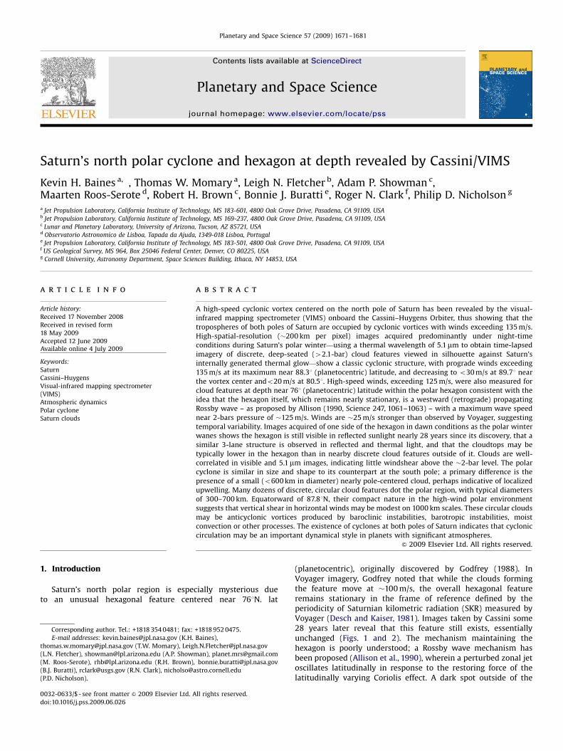
Fig. 2. Set of four high-spatial-resolution 5.1-mm mosaics of Saturn’s north polar region, photometrically inverted to show clouds as bright features. These near-nadir views

(sub-spacecraft latitude: 64–751) were acquired progressively on June 15, 2008 over a 6-h period from close range (as close as 224,000 km above the 1-bar level), yielding

clear polar views with up to 112 km/pixel resolution. Arrows point to clouds at three different latitudes, showing that winds are prograde and vary widely in speed over

latitude within the vortex.

K.H. Baines et al. / Planetary and Space Science 57 (2009) 1671–16811672

hexagon has been suggested as the source of the perturbation(Allison et al., 1990). Such a feature was seen repeatedly morethan a decade later in ground-based and Hubble Space Telescopeimagery (S�anchez-Lavega et al., 1993, 1997) but not in recentCassini/VIMS imagery (e.g., Fig. 1 and 2). As well, no evidence of

such a feature was observed in Cassini/CIRS infrared imageryobtained in March, 2007 (Fletcher et al., 2008).

Thus far, little information has been obtained about the farnorth, inside the hexagon. In particular, sparse information existson dynamical features that might bear on the processes forming

ARTICLE IN PRESS

K.H. Baines et al. / Planetary and Space Science 57 (2009) 1671–1681 1673

and maintaining the hexagon. As well, although a cyclonic hotvortex has been demonstrated to exist at the north pole in theupper troposphere and stratosphere by thermal-IR imaging(Fletcher et al., 2008), it is not known whether the vortexdemonstrates cloud morphologies and wind speeds similar tothe south polar cyclone (Dyudina et al., 2008, 2009).

-20.00.020.040.060.080.0100.0120.0140.0160.0

Planetocentric Latitude65.00 70.00 75.00 80.00 85.00 90.00

Zona

l Win

d (m

/s)

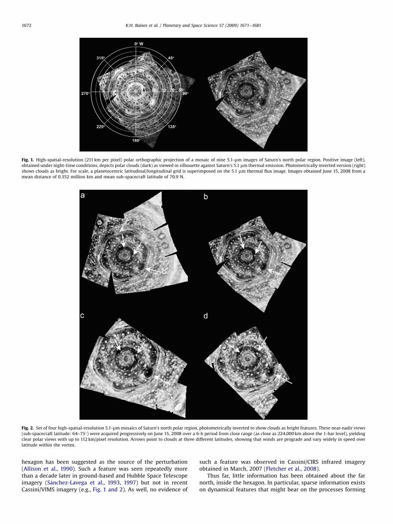
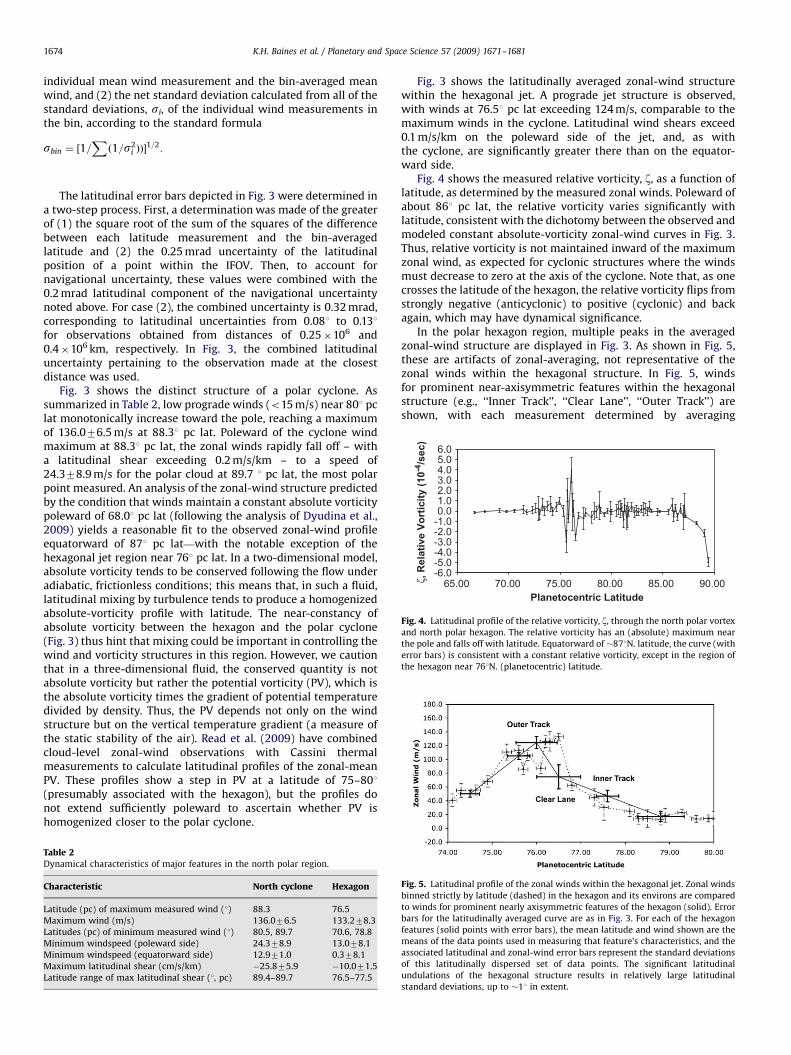
Fig. 3. Latitudinal profile of the north polar zonal winds (filled points with error

bars). Model wind profiles assuming constant absolute-vorticity poleward of

latitude fo yield the smooth curves, with fo ¼ 68.01 (upper, long-dashed curve)

and 69.51 (lower, dotted curve). Displayed error bars for the zonal winds are

explained in the text.

2. Observations and zonal-wind results

We report the first measurements of zonal winds throughoutthe north polar region, showing that a cyclonic vortex exists at thepole. These observations complement cloud tracking performedon VIMS images at lower latitudes (Choi et al., 2009). As shown inTable 1, mosaics of the polar region north of �701N were acquiredfour times on June 15–16, 2008 by the visual-infrared mappingspectrometer (VIMS) onboard the Cassini spacecraft orbitingSaturn. These mosaics were obtained at high-spatial-resolution(as small as 122 km in the instrument’s instantaneous field ofview, IFOV) over a range 0.224–0.442 million km above the cloudsfrom a vantage point high over northern latitudes (sub-spacecraftlatitudes of 641–751 N. latitude). While, typically, the VIMSinstrument simultaneously acquires images in 352 wavelengthbands from 0.35 to 5.1mm (c.f. Brown et al., 2004 for aninstrument review), we concentrate here on 5.1-mm thermalimagery and associated 4.6–5.1-mm spectra observable under thepredominantly night-time conditions of the north polar regionextant in June, 2008.

All images were photometrically and geometrically calibrated,including de-spiking and flat-fielding, using the well-developedprocedures of the VIMS Science Team as outlined in Barnes et al.(2007). In particular, images were geometrically calibrated usingthe ISIS software procedures (Gaddis et al., 1997) at the VIMS dataprocessing center at the University of Arizona, using the post-observation Cassini Mission SPICE kernels generated by NASA/JPL.A 0.2-mrad navigational uncertainty in both the latitudinal andlongitudinal components was adopted in the analysis of featureposition and zonal wind, as determined in a test of VIMS latitude/longitude assignments against those determined by RADAR, takenas ground truth, for an array of features on Titan (LawrenceSoderblom, personal communication).

As shown in Fig. 1, the 5.1-mm thermal imagery reveals zonallyoriented structures in the polar region, virtually all the way northto the pole. A polar ring of clouds is observed extending from87.81N to 88.61N planetocentric (pc) latitude. A 5-mm-bright ring– denoting a region of reduced aerosol opacity – extends from 831to 86.81 pc lat. At the time of these observations, the pole itselfwas occupied by a discrete cloud feature some 600 km indiameter. The center of this polar cloud is located at 89.71, offsetsome 300 km from the exact pole. Many dozens of similarlyshaped and size cloud features dot the polar region, occupyingabout 30% of the region.

Table 1Summary of observations.

Mosaic # # of VIMS frames in mosaic Start time of first frame En

North pole

1 9 6/15/08 16:05 6/1

2 9 6/15/08 17:48 6/1

3 12 6/15/08 20:35 6/1

4 12 6/15/08 22:39 6/1

South pole

1 10 6/16/08 14:51 6/1

Near 761 pc lat, the polar hexagon originally discovered byGodfrey (1988) is observed. Here, it appears predominantly as twodistinctive cloud ‘‘tracks’’ separated by a nearly cloud-free track.This complex of three hexagonal tracks extends over about 31 oflatitude at any single longitude.

We determined the polar zonal windfield from measurementof the time-varying longitudes of these cloud features as observedin four mosaics obtained over an 8.5-h period. As shown in Fig. 2,many clouds change their longitudinal position noticeablybetween images, particularly near the pole. Other clouds, suchas those near 801 pc lat, remain nearly stationary.

The resulting zonal-wind profile over latitude is shown inFig. 3. For each of 110 cloud points measured, the mean wind wasdetermined by a linear fit of the longitudinal position of thefeature vs. time, following the LINFIT procedure of Bevington(1969). At latitudes poleward of 801 pc lat, the longitudinalpositions of features were measured in all four mosaics.Equatorward of 801 pc lat, features were frequently observedand measured in just two or three mosaics. The longitudinaluncertainty was determined from two factors: the uncertainty of0.25 mrad for the location of a bright point within the VIMS 0.5-wide IFOV, and the 0.2 mrad uncertainty in the longitudinalcomponent of navigation for a VIMS pixel noted earlier. Together,these effects lead to a 0.32 mrad uncertainty associated with eachlongitudinal (and latitudinal) position measurement. Theseuncertainties fold into the determination of the uncertainty ofthe slope of the linear fit to the time–longitude data, therebyyielding an uncertainty for each zonal-wind measurement. InFig. 3, the displayed zonal-wind measurements are averaged overall observations within a latitude bin 0.21 wide, encompassing,typically, 2–3 points. For each binned point, the zonal-winduncertainty, sbin, is determined by the greater of (1) the standarddeviation calculated in the standard fashion, involving the squareroot of the sum of the squares of the difference between each

d time of last frame Range at start (103 km) Sub-S/C latitude (1, pc)

5/08 17:38 422 64.9

5/08 19:19 374 69.2

5/08 22:27 290 75.3

6/08 0:31 224 70.9

6/08 17:21 405 �48.3

ARTICLE IN PRESS

-6.0-5.0-4.0-3.0-2.0-1.00.01.02.03.04.05.06.0

65.00Planetocentric Latitude

ζ, R

elat

ive

Vort

icity

(10-4

/sec

)

70.00 75.00 80.00 85.00 90.00

Fig. 4. Latitudinal profile of the relative vorticity, z, through the north polar vortex

and north polar hexagon. The relative vorticity has an (absolute) maximum near

the pole and falls off with latitude. Equatorward of �871N. latitude, the curve (with

error bars) is consistent with a constant relative vorticity, except in the region of

the hexagon near 761N. (planetocentric) latitude.

K.H. Baines et al. / Planetary and Space Science 57 (2009) 1671–16811674

individual mean wind measurement and the bin-averaged meanwind, and (2) the net standard deviation calculated from all of thestandard deviations, si, of the individual wind measurements inthe bin, according to the standard formula

sbin ¼ ½1=Xð1=s2

i ÞÞ�1=2:

The latitudinal error bars depicted in Fig. 3 were determined ina two-step process. First, a determination was made of the greaterof (1) the square root of the sum of the squares of the differencebetween each latitude measurement and the bin-averagedlatitude and (2) the 0.25 mrad uncertainty of the latitudinalposition of a point within the IFOV. Then, to account fornavigational uncertainty, these values were combined with the0.2 mrad latitudinal component of the navigational uncertaintynoted above. For case (2), the combined uncertainty is 0.32 mrad,corresponding to latitudinal uncertainties from 0.081 to 0.131for observations obtained from distances of 0.25�106 and0.4�106 km, respectively. In Fig. 3, the combined latitudinaluncertainty pertaining to the observation made at the closestdistance was used.

Fig. 3 shows the distinct structure of a polar cyclone. Assummarized in Table 2, low prograde winds (o15 m/s) near 801 pclat monotonically increase toward the pole, reaching a maximumof 136.076.5 m/s at 88.31 pc lat. Poleward of the cyclone windmaximum at 88.31 pc lat, the zonal winds rapidly fall off – witha latitudinal shear exceeding 0.2 m/s/km – to a speed of24.378.9 m/s for the polar cloud at 89.7 1 pc lat, the most polarpoint measured. An analysis of the zonal-wind structure predictedby the condition that winds maintain a constant absolute vorticitypoleward of 68.01 pc lat (following the analysis of Dyudina et al.,2009) yields a reasonable fit to the observed zonal-wind profileequatorward of 871 pc lat—with the notable exception of thehexagonal jet region near 761 pc lat. In a two-dimensional model,absolute vorticity tends to be conserved following the flow underadiabatic, frictionless conditions; this means that, in such a fluid,latitudinal mixing by turbulence tends to produce a homogenizedabsolute-vorticity profile with latitude. The near-constancy ofabsolute vorticity between the hexagon and the polar cyclone(Fig. 3) thus hint that mixing could be important in controlling thewind and vorticity structures in this region. However, we cautionthat in a three-dimensional fluid, the conserved quantity is notabsolute vorticity but rather the potential vorticity (PV), which isthe absolute vorticity times the gradient of potential temperaturedivided by density. Thus, the PV depends not only on the windstructure but on the vertical temperature gradient (a measure ofthe static stability of the air). Read et al. (2009) have combinedcloud-level zonal-wind observations with Cassini thermalmeasurements to calculate latitudinal profiles of the zonal-meanPV. These profiles show a step in PV at a latitude of 75–801(presumably associated with the hexagon), but the profiles donot extend sufficiently poleward to ascertain whether PV ishomogenized closer to the polar cyclone.

Table 2Dynamical characteristics of major features in the north polar region.

Characteristic North cyclone Hexagon

Latitude (pc) of maximum measured wind (1) 88.3 76.5

Maximum wind (m/s) 136.076.5 133.278.3

Latitudes (pc) of minimum measured wind (1) 80.5, 89.7 70.6, 78.8

Minimum windspeed (poleward side) 24.378.9 13.078.1

Minimum windspeed (equatorward side) 12.971.0 0.378.1

Maximum latitudinal shear (cm/s/km) �25.875.9 �10.071.5

Latitude range of max latitudinal shear (1, pc) 89.4–89.7 76.5–77.5

Fig. 3 shows the latitudinally averaged zonal-wind structurewithin the hexagonal jet. A prograde jet structure is observed,with winds at 76.51 pc lat exceeding 124 m/s, comparable to themaximum winds in the cyclone. Latitudinal wind shears exceed0.1 m/s/km on the poleward side of the jet, and, as withthe cyclone, are significantly greater there than on the equator-ward side.

Fig. 4 shows the measured relative vorticity, z, as a function oflatitude, as determined by the measured zonal winds. Poleward ofabout 861 pc lat, the relative vorticity varies significantly withlatitude, consistent with the dichotomy between the observed andmodeled constant absolute-vorticity zonal-wind curves in Fig. 3.Thus, relative vorticity is not maintained inward of the maximumzonal wind, as expected for cyclonic structures where the windsmust decrease to zero at the axis of the cyclone. Note that, as onecrosses the latitude of the hexagon, the relative vorticity flips fromstrongly negative (anticyclonic) to positive (cyclonic) and backagain, which may have dynamical significance.

In the polar hexagon region, multiple peaks in the averagedzonal-wind structure are displayed in Fig. 3. As shown in Fig. 5,these are artifacts of zonal-averaging, not representative of thezonal winds within the hexagonal structure. In Fig. 5, windsfor prominent near-axisymmetric features within the hexagonalstructure (e.g., ‘‘Inner Track’’, ‘‘Clear Lane’’, ‘‘Outer Track’’) areshown, with each measurement determined by averaging

Fig. 5. Latitudinal profile of the zonal winds within the hexagonal jet. Zonal winds

binned strictly by latitude (dashed) in the hexagon and its environs are compared

to winds for prominent nearly axisymmetric features of the hexagon (solid). Error

bars for the latitudinally averaged curve are as in Fig. 3. For each of the hexagon

features (solid points with error bars), the mean latitude and wind shown are the

means of the data points used in measuring that feature’s characteristics, and the

associated latitudinal and zonal-wind error bars represent the standard deviations

of this latitudinally dispersed set of data points. The significant latitudinal

undulations of the hexagonal structure results in relatively large latitudinal

standard deviations, up to �11 in extent.

ARTICLE IN PRESS

K.H. Baines et al. / Planetary and Space Science 57 (2009) 1671–1681 1675

numerous observations around the hexagon. Due to thelatitudinally undulating nature of the hexagon, measurementsover a relatively wide variety of latitudes (up to 11) are used todetermine the mean wind value. The results of such a hexagon-feature analysis shows that the region is occupied by a single jetwith maximum mean zonal wind of 124.578.7 m/s located in theouter track of the hexagon. This is some 25 m/s greater than thezonal winds reported by Godfrey (1988) from daytime cloudtopimagery, located some 75 km above the lower-level clouds trackedhere, indicating a vertical shear of about 0.3 m/s/km in thetroposphere between approximately 0.5 and 2-bars if zonal windsare temporally invariant in the polar hexagon. Alternatively, if theobserved clouds are the same entities in visible light and at depth,as seems to be the case based on the co-alignment of the thermaland visible cloudtop features presented here (see below), andif the cloudtops are at the same altitude as the (unmeasured)cloudtops seen in reflected sunlight by Voyager, then these newwind measurements indicate time-variable winds in the hexagon.New measurements of visible cloud winds should be forthcomingas the sun rises over the hexagon, allowing some clarification ofthis issue.

That the clouds seen in reflected sunlight are the same as atdepth has not yet been clearly established, as, in the summer of

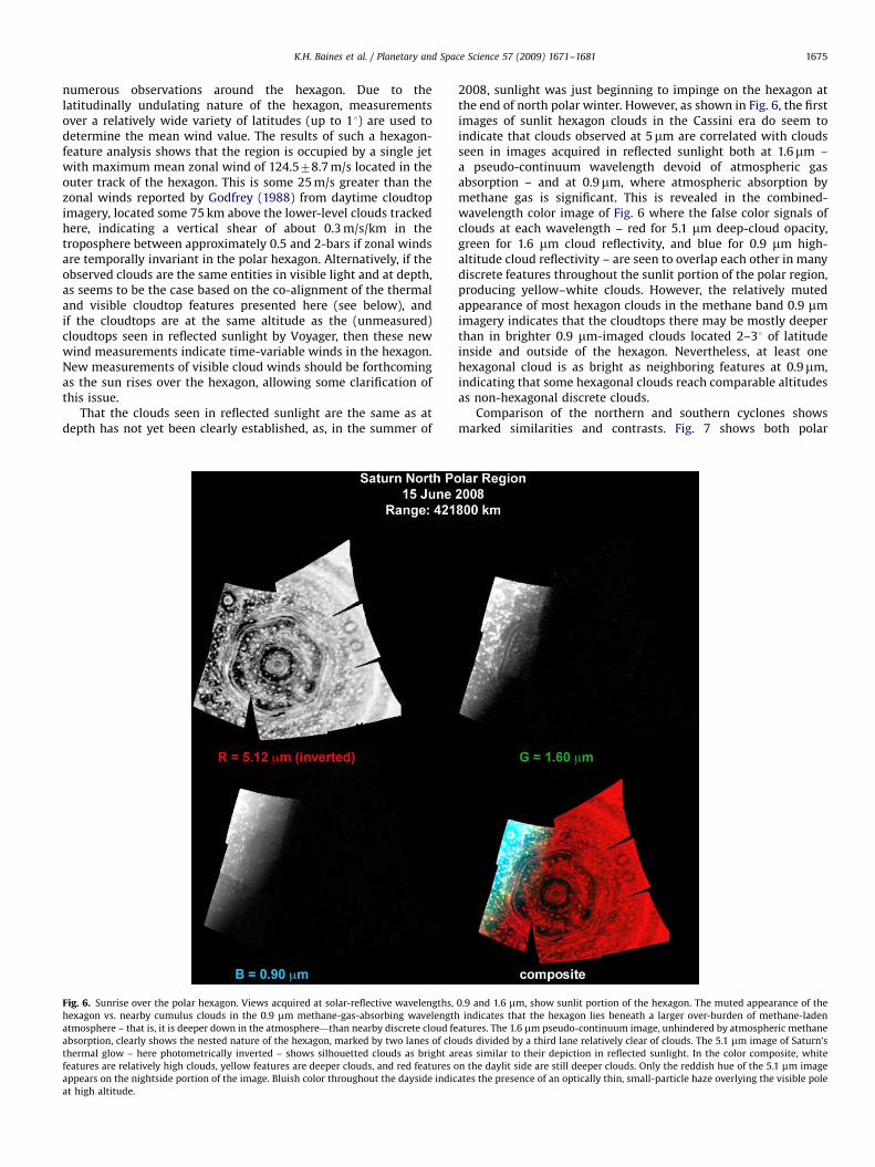
Fig. 6. Sunrise over the polar hexagon. Views acquired at solar-reflective wavelengths,

hexagon vs. nearby cumulus clouds in the 0.9 mm methane-gas-absorbing wavelength

atmosphere – that is, it is deeper down in the atmosphere—than nearby discrete cloud fe

absorption, clearly shows the nested nature of the hexagon, marked by two lanes of clo

thermal glow – here photometrically inverted – shows silhouetted clouds as bright ar

features are relatively high clouds, yellow features are deeper clouds, and red features o

appears on the nightside portion of the image. Bluish color throughout the dayside indic

at high altitude.

2008, sunlight was just beginning to impinge on the hexagon atthe end of north polar winter. However, as shown in Fig. 6, the firstimages of sunlit hexagon clouds in the Cassini era do seem toindicate that clouds observed at 5mm are correlated with cloudsseen in images acquired in reflected sunlight both at 1.6mm –a pseudo-continuum wavelength devoid of atmospheric gasabsorption – and at 0.9mm, where atmospheric absorption bymethane gas is significant. This is revealed in the combined-wavelength color image of Fig. 6 where the false color signals ofclouds at each wavelength – red for 5.1 mm deep-cloud opacity,green for 1.6 mm cloud reflectivity, and blue for 0.9 mm high-altitude cloud reflectivity – are seen to overlap each other in manydiscrete features throughout the sunlit portion of the polar region,producing yellow–white clouds. However, the relatively mutedappearance of most hexagon clouds in the methane band 0.9 mmimagery indicates that the cloudtops there may be mostly deeperthan in brighter 0.9 mm-imaged clouds located 2–31 of latitudeinside and outside of the hexagon. Nevertheless, at least onehexagonal cloud is as bright as neighboring features at 0.9mm,indicating that some hexagonal clouds reach comparable altitudesas non-hexagonal discrete clouds.

Comparison of the northern and southern cyclones showsmarked similarities and contrasts. Fig. 7 shows both polar

0.9 and 1.6 mm, show sunlit portion of the hexagon. The muted appearance of the

indicates that the hexagon lies beneath a larger over-burden of methane-laden

atures. The 1.6 mm pseudo-continuum image, unhindered by atmospheric methane

uds divided by a third lane relatively clear of clouds. The 5.1 mm image of Saturn’s

eas similar to their depiction in reflected sunlight. In the color composite, white

n the daylit side are still deeper clouds. Only the reddish hue of the 5.1 mm image

ates the presence of an optically thin, small-particle haze overlying the visible pole

ARTICLE IN PRESS

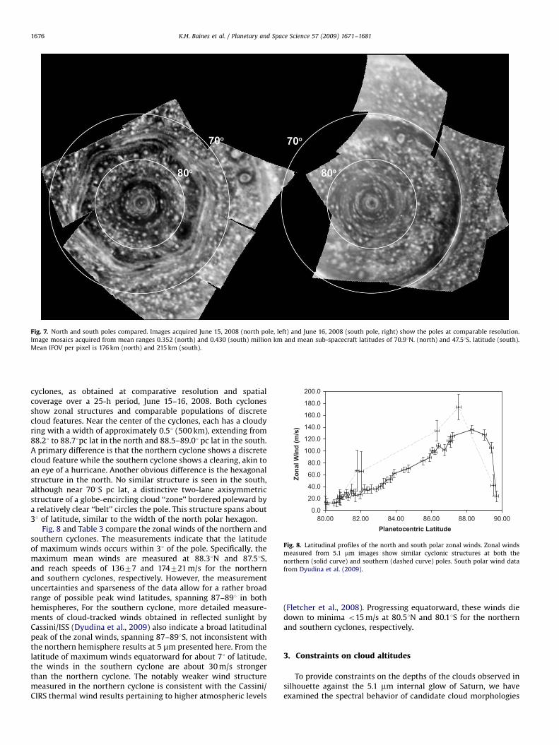
Fig. 7. North and south poles compared. Images acquired June 15, 2008 (north pole, left) and June 16, 2008 (south pole, right) show the poles at comparable resolution.

Image mosaics acquired from mean ranges 0.352 (north) and 0.430 (south) million km and mean sub-spacecraft latitudes of 70.91N. (north) and 47.51S. latitude (south).

Mean IFOV per pixel is 176 km (north) and 215 km (south).

0.0

20.0

40.0

60.0

80.0

100.0

120.0

140.0

160.0

180.0

200.0

80.00 82.00 84.00 86.00 88.00 90.00Planetocentric Latitude

Zona

l Win

d (m

/s)

Fig. 8. Latitudinal profiles of the north and south polar zonal winds. Zonal winds

measured from 5.1 mm images show similar cyclonic structures at both the

northern (solid curve) and southern (dashed curve) poles. South polar wind data

from Dyudina et al. (2009).

K.H. Baines et al. / Planetary and Space Science 57 (2009) 1671–16811676

cyclones, as obtained at comparative resolution and spatialcoverage over a 25-h period, June 15–16, 2008. Both cyclonesshow zonal structures and comparable populations of discretecloud features. Near the center of the cyclones, each has a cloudyring with a width of approximately 0.51 (500 km), extending from88.21 to 88.71pc lat in the north and 88.5–89.01 pc lat in the south.A primary difference is that the northern cyclone shows a discretecloud feature while the southern cyclone shows a clearing, akin toan eye of a hurricane. Another obvious difference is the hexagonalstructure in the north. No similar structure is seen in the south,although near 701S pc lat, a distinctive two-lane axisymmetricstructure of a globe-encircling cloud ‘‘zone’’ bordered poleward bya relatively clear ‘‘belt’’ circles the pole. This structure spans about31 of latitude, similar to the width of the north polar hexagon.

Fig. 8 and Table 3 compare the zonal winds of the northern andsouthern cyclones. The measurements indicate that the latitudeof maximum winds occurs within 31 of the pole. Specifically, themaximum mean winds are measured at 88.31N and 87.51S,and reach speeds of 13677 and 174721 m/s for the northernand southern cyclones, respectively. However, the measurementuncertainties and sparseness of the data allow for a rather broadrange of possible peak wind latitudes, spanning 87–891 in bothhemispheres, For the southern cyclone, more detailed measure-ments of cloud-tracked winds obtained in reflected sunlight byCassini/ISS (Dyudina et al., 2009) also indicate a broad latitudinalpeak of the zonal winds, spanning 87–891S, not inconsistent withthe northern hemisphere results at 5 mm presented here. From thelatitude of maximum winds equatorward for about 71 of latitude,the winds in the southern cyclone are about 30 m/s strongerthan the northern cyclone. The notably weaker wind structuremeasured in the northern cyclone is consistent with the Cassini/CIRS thermal wind results pertaining to higher atmospheric levels

(Fletcher et al., 2008). Progressing equatorward, these winds diedown to minima o15 m/s at 80.51N and 80.11S for the northernand southern cyclones, respectively.

3. Constraints on cloud altitudes

To provide constraints on the depths of the clouds observed insilhouette against the 5.1 mm internal glow of Saturn, we haveexamined the spectral behavior of candidate cloud morphologies

ARTICLE IN PRESS

Table 3Comparison of north vs. south polar cyclones.

Characteristic North cyclone South cyclone

Latitude (pc) of maximum measured wind (1) 88.3 87.5

Maximum wind (m/s) 136.076.5 174.0721.1

Central eye wind (m/s) 24.378.9 42.2717.7

Central eye latitude 89.7 89.5

Latitude (pc) of minimum measured wind (1) 80.5 80.1

Minimum windspeed 12.971.0 10.574.4

Eye Latitudinal shear (cm/s/km) �25.875.9 �6.471.3

Mean latitudinal shear 82–871 (cm/s/km) 1.870.2 1.970.7

Fig. 9. North polar feature identification. Depicted are the nine 5-mm-dark clouds

and 5-mm-bright clearings modeled with the NEMESIS radiative transfer code.

K.H. Baines et al. / Planetary and Space Science 57 (2009) 1671–1681 1677

with the NEMESIS radiative transfer and retrieval code (Irwinet al., 2008). In particular, we examined two types of cloudmorphologies. First, we examined a two-cloud model, whereintwo physically thin but potentially optically thick clouds wereplaced at two different levels in the atmosphere. In the uppertroposphere, a putative ammonia (NH3) cloud was placed at1.4-bar, the condensation level of ammonia pertaining to the solarmixing ratio of N/H (Atreya et al., 1999). Below this cloud, weplaced a second, compact, putative ammonium hydrosulfide(NH4SH) cloud for which the precise pressure level was deter-mined by the spectral analysis, as were as well the 5 mm opacitiesof both clouds. A wavelength-independent extinction coefficientwas adopted for both clouds.

In the second cloud morphology examined in our study, weassumed a single physically and optically thick cloud for whichthe cloudbase and 5 mm opacity are determined by the observa-tions. In this model, the cloud was assumed to extend from itscloudbase upward to the 75-mbar level, with a uniform verticaldistribution of opacity with pressure (i.e., equivalent to a particle-to-gas scale-height ratio of unity).

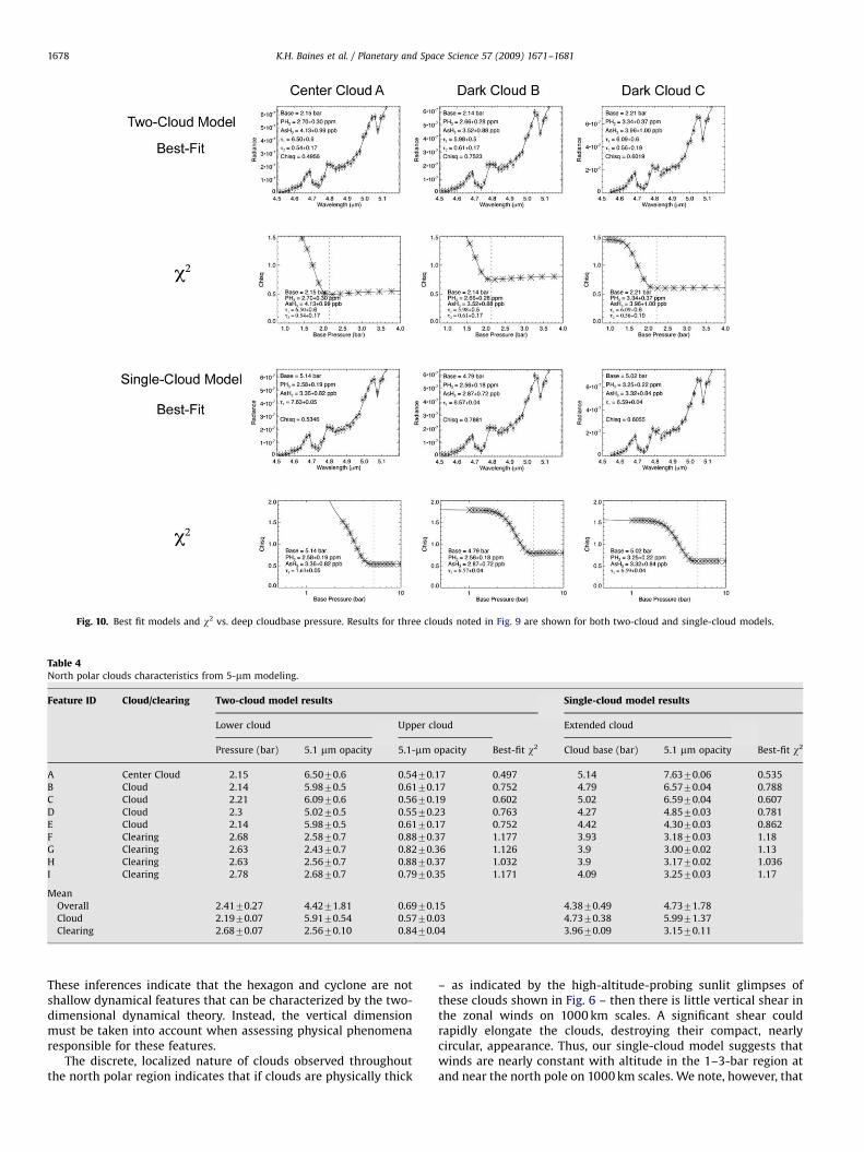
We analyzed nine specific spectra consisting of five 5-mm-darkcloudy and four 5-mm-bright less opaque regions denoted inFig. 9. Fig. 10 shows representative results for three cloudyregions, depicting the best-model fits and the variation of w2 foreach of the two morphologies. As a function of deep-cloudpressure, the fitting parameter, w2, diminishes greatly for deep

clouds below the 2- and 3-bar level for the two-cloud and single-cloud model, respectively. Best-fit results for all nine regions areshown in Table 4. For both morphologies, and for all regionsanalyzed, each of our analyses demands an optically thick cloud inthe lower troposphere at and below the 2.1- and 3.9-bar pressurelevel for the two-cloud and single-cloud model, respectively. Forthe deep cloud, there are distinct dichotomies between cloudyand relatively clear regions, as noted in the bottom rows of Table 4and shown graphically in Fig. 11. For both morphologies, the 5-mmopacity of cloudy regions is twice that of relatively clear regions.In the two-cloud model, the deep optically thick cloud is about 0.5bar higher in altitude in 5-mm-dark regions than in less opaque5-mm-bright regions. In contrast, for the single-cloud morphology,the base of the deep cloud is about 0.7 bar deeper in cloudyvs. relatively clear regions, i.e., at �4.7 vs. �4.0 bar in cloudy vs.relatively clear regions.

In the two-cloud model, similar 5-mm opacities are found forthe upper cloud in both cloudy and relatively clear regions, i.e.,�0.57 and �0.84 for the 5-mm-dark and bright regions, respec-tively. Thus, the two-cloud morphology suggests that a relativelyuniform cloud layer covers the north polar region, whose opacityis a factor of 4–8 less than the underlying deep cloud. Whilewe modeled this relatively optically thin cloud as occurringat the 1.4-bar ammonia condensation level, our analysis does notconstrain the altitude. Thus, this nearly uniform cloud layer couldbe almost anywhere above the 1.4-bar level. As the sun rises overthis region in 2009, the altitude, visual opacity, and othercharacteristics of the upper-level cloud layer should be discern-able in both VIMS spectral imagery and Imaging Sub-System (ISS)images multi-filter images.

In summary, our spectral analysis of two distinct cloudmorphologies indicates that 5-mm optically thick clouds arelocated relatively deep in the atmosphere, at or below the2.1-bar level, at depths below the ammonia condensation level.Thus, these deep clouds are not comprised of ammonia, but ratherlikely either ammonia hydrosulfide and/or water, the nexttwo condensibles predicted for the deep atmosphere of Saturn(Weidenschilling and Lewis, 1973; Atreya et al., 1999).

4. Dynamical implications and conclusion

The north polar cyclone together with its southern counterpart(Dyudina et al., 2008) are the first two polar cyclonic featuresdiscovered in the giant atmospheres of the outer solar system.Cyclones exist at both poles of Venus (e.g., Suomi and Limaye,1978; Limaye, 2007; Limaye et al., 2009), and polar vortices havebeen observed on Mars and Earth as well. The high-latitude jetson Neptune, which peak at a latitude of �701, could perhaps beviewed as circumpolar vortices, although they are much larger inlatitudinal extent than the polar vortex identified here. Thus, largecyclonic features appear to be not an uncommon dynamical modeof polar dynamics in planets with significant atmospheres.

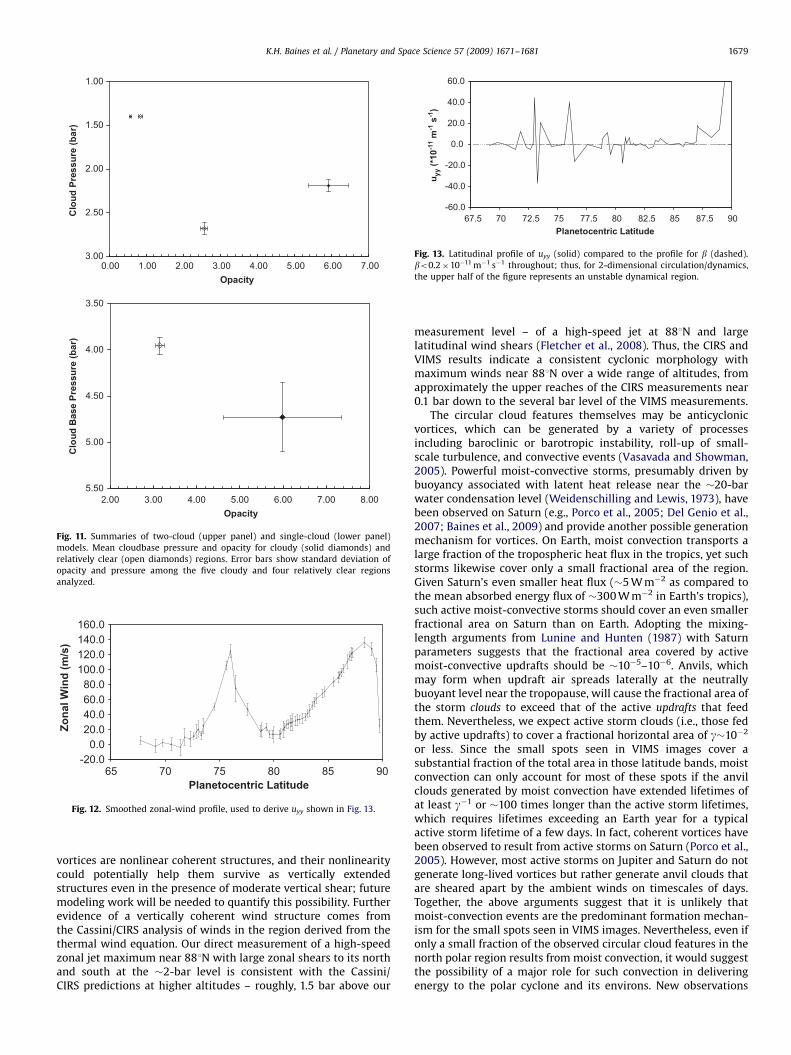
To investigate the two-dimensional dynamical stability of thenorth polar region, we examined the two-dimensional stabilitycriterion which compares the second meridional derivative ofzonal velocity, uyy, with the meridional derivative of the Coriolisforce (df/dy, or b). For more accurate analysis of differentialsover small distances and with non-insignificant error bars, wesmoothed the zonal velocity curve of Fig. 3 using spline fits andthe hexagonal zonal winds shown in Fig. 5. Fig. 12 shows theresulting smoothed zonal-wind profile for the north polar region,while Fig. 13 shows the resulting latitudinal profile of uyy

compared to b. Over much of the region, uyy exceeds b by morethan an order of magnitude, consistent with earlier inferencesfrom Voyager observations (Godfrey, 1988; Allison et al., 1990).

ARTICLE IN PRESS

Fig. 10. Best fit models and w2 vs. deep cloudbase pressure. Results for three clouds noted in Fig. 9 are shown for both two-cloud and single-cloud models.

Table 4North polar clouds characteristics from 5-mm modeling.

Feature ID Cloud/clearing Two-cloud model results Single-cloud model results

Lower cloud Upper cloud Extended cloud

Pressure (bar) 5.1 mm opacity 5.1-mm opacity Best-fit w2 Cloud base (bar) 5.1 mm opacity Best-fit w2

A Center Cloud 2.15 6.5070.6 0.5470.17 0.497 5.14 7.6370.06 0.535

B Cloud 2.14 5.9870.5 0.6170.17 0.752 4.79 6.5770.04 0.788

C Cloud 2.21 6.0970.6 0.5670.19 0.602 5.02 6.5970.04 0.607

D Cloud 2.3 5.0270.5 0.5570.23 0.763 4.27 4.8570.03 0.781

E Cloud 2.14 5.9870.5 0.6170.17 0.752 4.42 4.3070.03 0.862

F Clearing 2.68 2.5870.7 0.8870.37 1.177 3.93 3.1870.03 1.18

G Clearing 2.63 2.4370.7 0.8270.36 1.126 3.9 3.0070.02 1.13

H Clearing 2.63 2.5670.7 0.8870.37 1.032 3.9 3.1770.02 1.036

I Clearing 2.78 2.6870.7 0.7970.35 1.171 4.09 3.2570.03 1.17

Mean

Overall 2.4170.27 4.4271.81 0.6970.15 4.3870.49 4.7371.78

Cloud 2.1970.07 5.9170.54 0.5770.03 4.7370.38 5.9971.37

Clearing 2.6870.07 2.5670.10 0.8470.04 3.9670.09 3.1570.11

K.H. Baines et al. / Planetary and Space Science 57 (2009) 1671–16811678

These inferences indicate that the hexagon and cyclone are notshallow dynamical features that can be characterized by the two-dimensional dynamical theory. Instead, the vertical dimensionmust be taken into account when assessing physical phenomenaresponsible for these features.

The discrete, localized nature of clouds observed throughoutthe north polar region indicates that if clouds are physically thick

– as indicated by the high-altitude-probing sunlit glimpses ofthese clouds shown in Fig. 6 – then there is little vertical shear inthe zonal winds on 1000 km scales. A significant shear couldrapidly elongate the clouds, destroying their compact, nearlycircular, appearance. Thus, our single-cloud model suggests thatwinds are nearly constant with altitude in the 1–3-bar region atand near the north pole on 1000 km scales. We note, however, that

ARTICLE IN PRESS

1.00

1.50

2.00

2.50

3.000.00 1.00 2.00 3.00 4.00 5.00 6.00 7.00

Opacity

Clo

ud P

ress

ure

(bar

)

3.50

4.00

4.50

5.00

5.502.00 3.00 4.00 5.00 6.00 7.00 8.00

Opacity

Clo

ud B

ase

Pres

sure

(bar

)

Fig. 11. Summaries of two-cloud (upper panel) and single-cloud (lower panel)

models. Mean cloudbase pressure and opacity for cloudy (solid diamonds) and

relatively clear (open diamonds) regions. Error bars show standard deviation of

opacity and pressure among the five cloudy and four relatively clear regions

analyzed.

-20.00.020.040.060.080.0100.0120.0140.0160.0

65Planetocentric Latitude

Zona

l Win

d (m

/s)

70 75 80 85 90

Fig. 12. Smoothed zonal-wind profile, used to derive uyy shown in Fig. 13.

-60.0

-40.0

-20.0

0.0

20.0

40.0

60.0

67.5 70 72.5 75 77.5 80 82.5 85 87.5 90Planetocentric Latitude

u yy

(*10

-11 m

-1 s

-1)

Fig. 13. Latitudinal profile of uyy (solid) compared to the profile for b (dashed).

bo0.2�10�11 m�1 s�1 throughout; thus, for 2-dimensional circulation/dynamics,

the upper half of the figure represents an unstable dynamical region.

K.H. Baines et al. / Planetary and Space Science 57 (2009) 1671–1681 1679

vortices are nonlinear coherent structures, and their nonlinearitycould potentially help them survive as vertically extendedstructures even in the presence of moderate vertical shear; futuremodeling work will be needed to quantify this possibility. Furtherevidence of a vertically coherent wind structure comes fromthe Cassini/CIRS analysis of winds in the region derived from thethermal wind equation. Our direct measurement of a high-speedzonal jet maximum near 881N with large zonal shears to its northand south at the �2-bar level is consistent with the Cassini/CIRS predictions at higher altitudes – roughly, 1.5 bar above our

measurement level – of a high-speed jet at 881N and largelatitudinal wind shears (Fletcher et al., 2008). Thus, the CIRS andVIMS results indicate a consistent cyclonic morphology withmaximum winds near 881N over a wide range of altitudes, fromapproximately the upper reaches of the CIRS measurements near0.1 bar down to the several bar level of the VIMS measurements.

The circular cloud features themselves may be anticyclonicvortices, which can be generated by a variety of processesincluding baroclinic or barotropic instability, roll-up of small-scale turbulence, and convective events (Vasavada and Showman,2005). Powerful moist-convective storms, presumably driven bybuoyancy associated with latent heat release near the �20-barwater condensation level (Weidenschilling and Lewis, 1973), havebeen observed on Saturn (e.g., Porco et al., 2005; Del Genio et al.,2007; Baines et al., 2009) and provide another possible generationmechanism for vortices. On Earth, moist convection transports alarge fraction of the tropospheric heat flux in the tropics, yet suchstorms likewise cover only a small fractional area of the region.Given Saturn’s even smaller heat flux (�5 W m�2 as compared tothe mean absorbed energy flux of �300 W m�2 in Earth’s tropics),such active moist-convective storms should cover an even smallerfractional area on Saturn than on Earth. Adopting the mixing-length arguments from Lunine and Hunten (1987) with Saturnparameters suggests that the fractional area covered by activemoist-convective updrafts should be �10�5–10�6. Anvils, whichmay form when updraft air spreads laterally at the neutrallybuoyant level near the tropopause, will cause the fractional area ofthe storm clouds to exceed that of the active updrafts that feedthem. Nevertheless, we expect active storm clouds (i.e., those fedby active updrafts) to cover a fractional horizontal area of g�10�2

or less. Since the small spots seen in VIMS images cover asubstantial fraction of the total area in those latitude bands, moistconvection can only account for most of these spots if the anvilclouds generated by moist convection have extended lifetimes ofat least g�1 or �100 times longer than the active storm lifetimes,which requires lifetimes exceeding an Earth year for a typicalactive storm lifetime of a few days. In fact, coherent vortices havebeen observed to result from active storms on Saturn (Porco et al.,2005). However, most active storms on Jupiter and Saturn do notgenerate long-lived vortices but rather generate anvil clouds thatare sheared apart by the ambient winds on timescales of days.Together, the above arguments suggest that it is unlikely thatmoist-convection events are the predominant formation mechan-ism for the small spots seen in VIMS images. Nevertheless, even ifonly a small fraction of the observed circular cloud features in thenorth polar region results from moist convection, it would suggestthe possibility of a major role for such convection in deliveringenergy to the polar cyclone and its environs. New observations

ARTICLE IN PRESS

K.H. Baines et al. / Planetary and Space Science 57 (2009) 1671–16811680

expected from the high-resolution ISS camera system onboardCassini should reveal much about the true nature of these featuresas the sun rises over the north polar region in 2009.

The north polar hexagon has now been observed repeatedly for27.6 years, corresponding to nearly a Saturnian year (29.4 years).Voyager observations in November 1980 and August 1981(Godfrey, 1988), ground-based observations in June, 1989(S�anchez-Lavega et al., 1993), and repeated Cassini/VIMS andCassini/CIRS observations since October, 2006 (Baines et al., 2007;Fletcher et al., 2008), have all shown the presence of thehexagonal feature. Both the long-term nature of the hexagonand its presence deep in the atmosphere at altitudes below the2-bar level indicate that this feature is not a consequence of solarinsolation effects but rather is associated with the global, non-seasonal circulation of Saturn.

The formation mechanism for the hexagon remains unclear.Allison et al. (1990) suggested that a planetary (i.e., westward-propagating Rossby) wave mechanism is responsible, whereinperturbations to the zonal flow induced by a large dark spotobserved 31 south of the hexagon (Godfrey, 1988) serves to causewavenumber 6 Rossby wave oscillations in the flow which appearas the straight-legged sides and curved corners of the high-latitude hexagon. This large (6000 km wide) dark spot wasobserved repeatedly over the years by Voyager in 1980/1981(Godfrey, 1988), ground-based imagery in 1990/1991 (S�anchez-Lavega et al., 1993), and 1992–1995 (S�anchez-Lavega et al., 1997).However, this feature does not appear in the high-resolutionimages presented here, nor in the Cassini/CIRS observations ofMarch 2007 (Fletcher et al., 2008), nor in any VIMS imagery of thenorth pole obtained during the mission beginning in October2006 (Baines et al., 2007 and Figs. 1,2). The apparent longevityof the hexagon in absence of the dark spot, thus, raises thepossibility that the dark spot was a by-product of hexagonformation (or perhaps even an unrelated feature altogether)rather than a cause of the hexagon.

Alternatively, it is possible that the hexagon results from aninstability of the flow at the hexagon latitude. Laboratoryexperiments motivated by Saturn’s hexagon (Aguiar et al., 2009),and numerical studies of terrestrial hurricanes (Schubert et al.,1999; Kossin and Schubert, 2001) show success in producingpolygons from a barotropic instability. Such an instability is ahorizontal shear instability that would convert kinetic energy of apre-existing fast jet (as exists at the hexagon latitude) into eddykinetic energy associated with the hexagon wave. Alternatively,it may be possible for the hexagon to result from a baroclinicinstability if latitudinal temperature gradients exist at thehexagon latitude. Such instabilities, which would convertpotential energy into kinetic energy, could help to pump thefast hexagon jet in addition to creating the hexagon wave.(An analogous mechanism was proposed for Saturn’s Ribbonwave by Godfrey and Moore, 1986.) Numerical simulations ofbaroclinic instabilities on gas giants show that such instabilitiescan indeed pump zonal jets (Lian and Showman, 2008; Williams,2003) and in some cases lead to wave structures on those jets thatcould appear polygonal if viewed from over the pole (Williams,2003). Note that both types of instabilities can also producecoherent vortices and thus could provide the explanation for theadjacent dark spot seen in Voyager, ground-based, and earlyCassini imagery.

Acknowledgments

We thank Cassini/VIMS team members John Ivens, FrankLeader, Dyer Lytle, Dan Moynihan, Virginia Pasek, Alan Stevenson,and Bob Watson for much help in the sequence generation,

instrument calibration, and data reduction of the maps andspectra used in this paper. We would like to thank Anthony DelGenio and an anonymous referee for their valuable comments.Much of the work described in this paper was carried out in partat the Jet Propulsion Laboratory, Pasadena, California, undercontract with the National Aeronautics and Space Administration.LNF was supported by an appointment to the NASA PostdoctoralProgram at the Jet Propulsion Laboratory, administered by OakRidge Associated Universities through a contract with NASA. Wethank Patrick Irwin and colleagues for the use of the Oxford-basedradiative transfer and retrieval code.

References

Aguiar, A.C.B., Read, P.L., Salter, T., Wordsworth, R.D., Yamazaki, Y.H., 2009. Alaboratory model of Saturn’s north polar hexagon. Icarus, submitted.

Allison, M., Godfrey, D.A., Beebe, R.F., 1990. A wave dynamical interpretation ofSaturn’s polar hexagon. Science 247, 1061–1063.

Atreya, S.K., Wong, M.H., Owen, T.C., Mahaffy, P.R., Niemann, H.B., de Pater, I.,Drossart, P., Encrenaz, T., 1999. A comparison of the atmospheres of Jupiter andSaturn: Deep atmospheric composition, cloud structure, vertical mixing, andorigin. Planet. Space Sci. 47, 1243–1262.

Baines, K.H., Momary, T.W., Temma, T., Buratti, B.J., Roos-Serote, M., Showman, A.,Brown, R.H., Clark, R.N., Nicholson, P.D., Atreya, S.K., Graham, J., Marquez, E., 2007.The structure of Saturn’s poles determined by Cassini/VIMS: Constraints on windsand horizontal and vertical cloud distributions. Bull. Amer. Astr. Soc. 38, 423.

Baines, K.H., Delitsky, M.L., Momary, T.W., Brown, R.H., Buratti, B.J., Clark, R.N.,Nicholson, P.D., 2009. Storm clouds on Saturn: Lightning-induced chemistryand associated materials consistent with Cassini/VIMS spectra. Planet. SpaceSci, this issue, doi:10.1016/j.pss.2009.06.025.

Barnes, J.W., Brown, R.H., Soderblom, L., Buratti, B.J., Sotin, C., Rodriguez, S., LeMouelic, S., Baines, K.H., Clark, R., Nicholson, P., 2007. Global-scale surfacespectral variations on Titan seen from Cassini/VIMS. Icarus 186, 242–258.

Bevington, P.R., 1969. Data Reduction and Error Analysis for the Physical Sciences.McGraw Hill, New York, pp. 104–105.

Brown, R.H., 21 Colleagues, 2004. The Cassini visual and infrared mappingspectrometer investigation. Space Sci. Rev. 115 (1–4), 111–168.

Choi, D.S., Showman, A.P., Brown, R.H., 2009. Cloud features and zonalwind measurements of Saturn’s atmosphere as observed by Cassini/VIMS.J. Geophys. Res., doi:10.1029/2008JE003254.

Del Genio, A.D., Coauthors, 2007. Saturn eddy momentum fluxes and convection:first estimates from Cassini images. Icarus 189, 479–492, doi:10.1016/j.icarus.2007.02.013.

Desch, M.D., Kaiser, M.L., 1981. Voyager measurements of the rotation period ofSaturn’s magnetic field. Geophys. Res. Lett. 8, 253–256.

Dyudina, U.A., Ingersoll, A.P., Ewald, S., Vasavada, A., West, R.A., Del Genio, A.,Barbara, J., Porco, C.C., Achterberg, R., Flasar, F., Simon-Miller, A., Fletcher, L.N.,2008. Dynamics of Saturn’s south polar vortex. Science 319, 1801.

Dyudina, U.A., Ingersoll, A.P., Ewald, S.P., Vasavada, A.R., West, R.A., Baines, K.H.,Momary, T.W., Del Genio, A.D., Barbara, J.M., Porco, C.C., Achterberg, R.K., Flasar,F.M., Simon-Miller, A.A., Fletcher, L.N., 2009. Saturn’s south polar vortexcompared to other large vortices in the solar system. Icarus 202, 240–248.

Fletcher, L.N., Irwin, P.G.J., Orton, G.S., Tenby, N.A., Achterberg, R.K., Bjoraker, G.L.,Read, P.L., Simon-Miller, A.A., Howett, C., de Kok, R., Bolwes, N., Calcutt, S.B.,Hesman, B., Flasar, F.M., 2008. Temperature and composition of Saturn’s polarhot spots and hexagon. Science 319, 70–82.

Gaddis, L., et al., 1997. An overview of the Integrated Software for ImagingSpectrometers (ISIS), Lunar and Planetary Institute Conference Abstracts, 28, 387.

Godfrey, D.A., 1988. A hexagonal feature around Saturn’s north pole. Icarus 76,335–356.

Godfrey, D.A., Moore, V., 1986. The Saturnian ribbon feature—a baroclinicallyunstable model. Icarus 68, 313–343.

Irwin, P.G.J., Teanby, N.A., de Kok, R., Fletcher, L.N., Howett, C.J.A., Tsang, C.C.C.,Wilson, C.F., Calcutt, S.B., Nixon, C.A., Parrish, P.D., 2008. The NEMESISplanetary atmosphere radiative transfer and retrieval tool. J. Quant. Spectrosc.Radiative Transfer 109, 1136–1150.

Kossin, J.P., Schubert, W.H., 2001. Mesovortices, polygonal flow patterns, and rapidpressure falls in hurricane-like vortices. J. Atmos. Sci. 58, 2196–2209.

Lian, Y., Showman, A.P., 2008. Deep jets on gas-giant planets. Icarus 194, 597–615,doi:10.1016/j.icarus.2007.10.014.

Limaye, S.S., 2007. Venus atmospheric circulation: known and unknown.J. Geophys. Res. 112, E04S09, doi:10.1029/2006JE002814.

Limaye, S.S., Kossin, J.P., Rozoff, C., Piccioni, G., Titov, D.V., Markiewicz, W.J., 2009.Vortex circulation on Venus: Dynamical similarities with terrestrial hurri-canes. Geophys. Res. Lett. 36, L04204, doi:10.1029/2008GL036093.

Lunine, J.I., Hunten, D.M., 1987. Moist convection and the abundance of water inthe troposphere of Jupiter. Icarus 69, 566–570.

Porco, C.C., 31 Colleagues, 2005. Cassini imaging science: initial results on Saturn’satmosphere. Science 307, 1243–1247.

Read, P.L., Conrath, B.J., Fletcher, L.N., Gierasch, P.J., Simon-Miller, A.A., Zuchowski,L.C., 2009. Mapping potential vorticity dynamics on Saturn: zonal mean

ARTICLE IN PRESS

K.H. Baines et al. / Planetary and Space Science 57 (2009) 1671–1681 1681

circulation from Cassini and Voyager data. Plane. Space Sci., this issue,doi:10.1016/j.pss.2009.03.004.

S�anchez-Lavega, A., Lecacheux, J., Colas, F., Lacques, P., 1993. Ground-basedobservations of Saturn’s North Polar spot and hexagon. Science 260, 329–332.

S�anchez-Lavega, A., Rojas, J.F., Acarreta, J.F., Lecacheux, J., Colas, F., Sada, P.V., 1997.New observations and studies of Saturn’s long-lived North Polar spot. Icarus128, 322–334.

Schubert, W.H., Montgomery, M.T., Taft, R.K., Guinn, T.A., Fulton, S.R., Kossin, J.P.,Edwards, J.P., 1999. Polygonal eyewalls, asymmetric eye contraction, andpotential vorticity mixing in hurricanes. J. Atmos. Sci. 56, 1197–1223.

Suomi, V.E., Limaye, S.S., 1978. Venus: further evidence of vortex circulation.Science 201, 1009–1011.

Vasavada, A.R., Showman, A.P., 2005. Jovian atmospheric dynamics: an updateafter Galileo and Cassini. Rep. Prog. Phys. 68, 1935–1996.

Weidenschilling, S.J., Lewis, J.S., 1973. Atmospheric and cloud structures of theJovian planets. Icarus 20, 465–476.

Williams, G.P., 2003. Jovian dynamics, part III: multiple, migrating, and equatorialjets. J. Atmos. Sci. 60, 1270–1296.