Embed Size (px)
Citation preview
Pivot Sampling in Dual-Pivot QuicksortExploiting Asymmetries in Yaroslavskiy’s Partitioning Scheme
Markus E. Nebel12†and Sebastian Wild1
1Computer Science Department, University of Kaiserslautern2Department of Mathematics and Computer Science, University of Southern Denmark
Abstract: The new dual-pivot Quicksort by Vladimir Yaroslavskiy — used in Oracle’s Java runtime library sinceversion 7 — features intriguing asymmetries in its behavior. They were shown to cause a basic variant of this algorithmto use less comparisons than classic single-pivot Quicksort implementations. In this paper, we extend the analysis tothe case where the two pivots are chosen as fixed order statistics of a random sample and give the precise leading termof the average number of comparisons, swaps and executed Java Bytecode instructions. It turns out that — unlike forclassic Quicksort, where it is optimal to choose the pivot as median of the sample — the asymmetries in Yaroslavskiy’salgorithm render pivots with a systematic skew more efficient than the symmetric choice. Moreover, the optimalskew heavily depends on the employed cost measure; most strikingly, abstract costs like the number of swaps andcomparisons yield a very different result than counting Java Bytecode instructions, which can be assumed most closelyrelated to actual running time.
Keywords: Quicksort, dual-pivot, Yaroslavskiy’s partitioning method, median of three, average case analysis
1 IntroductionQuicksort is one of the most efficient comparison-based sorting algorithms and is thus widely used inpractice, for example in the sort implementations of the C++ standard library and Oracle’s Java runtimelibrary. Almost all practical implementations are based on the highly tuned version of Bentley and McIlroy(1993), often equipped with the strategy of Musser (1997) to avoid quadratic worst case behavior. The Javaruntime environment was no exception to this — up to version 6. With version 7 released in 2009, however,Oracle broke with this tradition and replaced its tried and tested implementation by a dual-pivot Quicksortwith a new partitioning method proposed by Vladimir Yaroslavskiy.
The decision was based on extensive running time experiments that clearly favored the new algorithm.This was particularly remarkable as earlier analyzed dual-pivot variants had not shown any potential forperformance gains over classic single-pivot Quicksort (Sedgewick, 1975; Hennequin, 1991). However,we could show for pivots from fixed array positions (i.e. no sampling) that Yaroslavskiy’s asymmetricpartitioning method beats classic Quicksort in the comparison model: asymptotically 1.9n lnn vs. 2n lnn
†The order of authors follows the Hardy-Littlewood rule, i.e., it is alphabetical by last name.
1365–8050 © 2005 Discrete Mathematics and Theoretical Computer Science (DMTCS), Nancy, France
arX
iv:1
403.
6602
v2 [
cs.D
S] 1
3 Ju
n 20
14
2 Markus E. Nebel and Sebastian Wild
comparisons on average (Wild and Nebel, 2012). As these savings are opposed by a large increase inthe number of swaps, the overall competition still remained open. To settle it, we compared two Javaimplementations of the Quicksort variants and found that Yaroslavskiy’s method actually executes moreJava Bytecode instructions on average (Wild et al., 2013b). A possible explanation why it still shows betterrunning times was recently given by Kushagra et al. (2014): Yaroslavskiy’s algorithm needs fewer scansover the array than classic Quicksort, and is thus more efficient in the external memory model.
Our analyses cited above ignore a very effective strategy in Quicksort: for decades, practical implemen-tations choose their pivots as median of a random sample of the input to be more efficient (both in terms ofaverage performance and in making worst cases less likely). Oracle’s Java 7 implementation also employsthis optimization: it chooses its two pivots as the tertiles of five sample elements. This equidistant choice isa plausible generalization, since selecting the pivot as median is known to be optimal for classic Quicksort(Sedgewick, 1975; Martínez and Roura, 2001).
However, the classic partitioning methods treat elements smaller and larger than the pivot in symmetricways — unlike Yaroslavskiy’s partitioning algorithm: depending on how elements relate to the two pivots,one of five different execution paths is taken in the partitioning loop, and these can have highly differentcosts! How often each of these five paths is taken depends on the ranks of the two pivots, which we canpush in a certain direction by selecting other order statistics of a sample than the tertiles. The partitioningcosts alone are then minimized if the cheapest execution path is taken all the time. This however leads tovery unbalanced distributions of sizes for the recursive calls, such that a trade-off between partitioningcosts and balance of subproblem sizes results.
We have demonstrated experimentally that there is potential to tune dual-pivot Quicksort using skewedpivots (Wild et al., 2013c), but only considered a small part of the parameter space. It will be the purposeof this paper to identify the optimal way to sample pivots by means of a precise analysis of theresulting overall costs, and to validate (and extend) the empirical findings that way.
Related work. Single-pivot Quicksort with pivot sampling has been intensively studied over the lastdecades (Emden, 1970; Sedgewick, 1975, 1977; Hennequin, 1991; Martínez and Roura, 2001; Neininger,2001; Chern and Hwang, 2001; Durand, 2003). We heavily profit from the mathematical foundations laidby these authors. There are scenarios where, even for the symmetric, classic Quicksort, a skewed pivot canyield benefits over median of k (Martínez and Roura, 2001; Kaligosi and Sanders, 2006). An importantdifference to Yaroslavskiy’s algorithm is, however, that the situation remains symmetric: a relative pivotrank α < 1
2 has the same effect as one with rank 1 − α. For dual-pivot Quicksort with an arbitrarypartitioning method, Aumüller and Dietzfelbinger (2013) establish a lower bound of asymptotically1.8n lnn comparisons and they also propose a partitioning method that attains this bound.
Outline. After listing some general notation, Section 3 introduces the subject of study. Section 4 collectsthe main analytical results of this paper, whose proof is divided into Sections 5, 6 and 7. Arguments inthe main text are kept concise, but the interested reader is provided with details in the appendix. Thealgorithmic consequences of our analysis are discussed in Section 8. Section 9 concludes the paper.
2 Notation and PreliminariesWe write vectors in bold font, for example t = (t1, t2, t3). For concise notation, we use expressions liket + 1 to mean element-wise application, i.e., t + 1 = (t1 + 1, t2 + 1, t3 + 1). By Dir(α), we denote arandom variable with Dirichlet distribution and shape parameter α = (α1, . . . , αd) ∈ Rd>0. Likewisefor parameters n ∈ N and p = (p1, . . . , pd) ∈ [0, 1]d with p1 + · · · + pd = 1, we write Mult(n,p) for
Pivot Sampling in Dual-Pivot Quicksort 3
a random variable with multinomial distribution with n trials. HypG(k, r, n) is a random variable withhypergeometric distribution, i.e., the number of red balls when drawing k times without replacement froman urn of n ∈ N balls, r of which are red, (where k, r ∈ {1, . . . , n}). Finally, U(a, b) is a random variableuniformly distributed in the interval (a, b), and B(p) is a Bernoulli variable with probability p to be 1. Weuse “D=” to denote equality in distribution.
As usual for the average case analysis of sorting algorithms, we assume the random permutation model,i.e., all elements are different and every ordering of them is equally likely. The input is given as array Aof length n and we denote the initial entries of A by U1, . . . , Un. We further assume that U1, . . . , Un arei. i. d. uniformly U(0, 1) distributed; as their ordering forms a random permutation (Mahmoud, 2000), thisassumption is without loss of generality. Some further notation specific to our analysis is introduced below;for reference, we summarize all notations used in this paper in Appendix A.
3 Generalized Yaroslavskiy QuicksortIn this section, we review Yaroslavskiy’s partitioning method and combine it with the pivot samplingoptimization to obtain what we call the Generalized Yaroslavskiy Quicksort algorithm. We leave someparts of the algorithm unspecified here, but give a full-detail implementation in the appendix. The reason isthat preservation of randomness is somewhat tricky to achieve in presence of pivot sampling, but vital forprecise analysis. The casual reader might content him- or herself with our promise that everything turnsout alright in the end; the interested reader is invited to follow our discussion of this issue in Appendix B.
3.1 Generalized Pivot SamplingOur pivot selection process is declaratively specified as follows, where t = (t1, t2, t3) ∈ N3 is a fixedparameter: choose a random sample V = (V1, . . . , Vk) of size k = k(t) := t1 + t2 + t3 + 2 from theelements and denote by (V(1), . . . , V(k)) the sorted (i) sample, i.e., V(1) ≤ V(2) ≤ · · · ≤ V(k). Then choosethe two pivots P := V(t1+1) and Q := V(t1+t2+2) such that they divide the sorted sample into three regionsof respective sizes t1, t2 and t3:
V(1) . . . V(t1)︸ ︷︷ ︸t1 elements
≤ V(t1+1)︸ ︷︷ ︸=P
≤ V(t1+2) . . . V(t1+t2+1)︸ ︷︷ ︸t2 elements
≤ V(t1+t2+2)︸ ︷︷ ︸=Q
≤ V(t1+t2+3) . . . V(k)︸ ︷︷ ︸t3 elements
. (3.1)
Note that by definition, P is the small(er) pivot and Q is the large(r) one. We refer to the k − 2 elementsof the sample that are not chosen as pivot as “sampled-out”; P and Q are the chosen pivots. All otherelements — those which have not been part of the sample — are referred to as ordinary elements. Pivotsand ordinary elements together form the set of partitioning elements, (because we exclude sampled-outelements from partitioning).
3.2 Yaroslavskiy’s Dual Partitioning MethodIn bird’s-eye view, Yaroslavskiy’s partitioning method consists of two indices, k and g, that start at theleft resp. right end of A and scan the array until they meet. Elements left of k are smaller or equal than Q,elements right of g are larger. Additionally, a third index ` lags behind k and separates elements smallerthan P from those between both pivots. Graphically speaking, the invariant of the algorithm is as follows:
P Q< P
`
≥ Qg
P ≤ ◦ ≤ Qk ←→ →
?
(i) In case of equal elements any possible ordering will do. However in this paper, we assume distinct elements.
4 Markus E. Nebel and Sebastian Wild
We write K and G for the sets of all indices that k resp. g attain in the course of the partitioning process.Moreover, we call an element small, medium, or large if it is smaller than P , between P and Q, or largerthan Q, respectively. The following properties of the algorithm are needed for the analysis, (see Wild andNebel (2012); Wild et al. (2013b) for details):
(Y1) Elements Ui, i ∈ K, are first compared with P . Only if Ui is not small, it is also compared to Q.
(Y2) Elements Ui, i ∈ G, are first compared with Q. If they are not large, they are also compared to P .
(Y3) Every small element eventually causes one swap to put it behind `.
(Y4) The large elements located in K and the non-large elements in G are always swapped in pairs.
For the number of comparisons we will thus need to count the large elements Ui with i ∈ K; we abbreviatetheir number by “l@K”. Similarly, s@K and s@G denote the number of small elements in k’s resp. g’srange.
When partitioning is finished, k and g have met and thus ` and g divide the array into three ranges,containing the small, medium resp. large (ordinary) elements, which are then sorted recursively. Forsubarrays with at most w elements, we switch to Insertionsort, (where w is constant and at least k). Theresulting algorithm, Generalized Yaroslavskiy Quicksort with pivot sampling parameter t = (t1, t2, t3)and Insertionsort threshold w, is henceforth called Y wt .
4 ResultsFor t ∈ N3 andHn the nth harmonic number, we define the discrete entropy H(t) of t as
H(t) =
3∑l=1
tl + 1
k + 1(Hk+1 −Htl+1) . (4.1)
The name is justified by the following connection between H(t) and the entropy function H∗ of informationtheory: for the sake of analysis, let k →∞, such that ratios tl/k converge to constants τl. Then
H(t) ∼ −3∑l=1
τl(ln(tl + 1)− ln(k + 1)
)∼ −
3∑l=1
τl ln(τl) =: H∗(τ ) . (4.2)
The first step follows from the asymptotic equivalenceHn ∼ ln(n) as n→∞. (4.2) shows that for large t,the maximum of H(t) is attained for τ1 = τ2 = τ3 = 1
3 . Now we state our main result:
Theorem 4.1 (Main theorem): Generalized Yaroslavskiy Quicksort with pivot sampling parameter t =(t1, t2, t3) performs on average Cn ∼ aC
H(t) n lnn comparisons and Sn ∼ aSH(t) n lnn swaps to sort a
random permutation of n elements, where
aC = 1 +t2 + 1
k + 1+
(2t1 + t2 + 3)(t3 + 1)
(k + 1)(k + 2)and aS =
t1 + 1
k + 1+
(t1 + t2 + 2)(t3 + 1)
(k + 1)(k + 2). (4.3)
Moreover, if the partitioning loop is implemented as in Appendix C of (Wild et al., 2013b), it executes onaverage BCn ∼ aBC
H(t) n lnn Java Bytecode instructions to sort a random permutation of size n with
aBC = 10 + 13t1 + 1
k + 1+ 5
t2 + 1
k + 1+ 11
(t1 + t2 + 2)(t3 + 1)
(k + 1)(k + 2)+
(t1 + 1)(t1 + t2 + 3)
(k + 1)(k + 2). (4.4)
Pivot Sampling in Dual-Pivot Quicksort 5
The following sections are devoted to the proof of Theorem 4.1. Section 5 sets up a recurrence of costsand characterizes the distribution of costs of one partitioning step. The expected values of the latter arecomputed in Section 6. Finally, Section 7 provides a generic solution to the recurrence of the expectedcosts; in combination with the expected partitioning costs, this concludes our proof.
5 Distributional Analysis5.1 Recurrence Equations of CostsLet us denote by Cn the costs of Y wt on a random permutation of size n— where different “cost measures”,like the number of comparisons, will take the place of Cn later. Cn is a non-negative random variablewhose distribution depends on n. The total costs decompose into those for the first partitioning step plus thecosts for recursively solving subproblems. As Yaroslavskiy’s partitioning method preserves randomness(see Appendix B), we can express the total costs Cn recursively in terms of the same cost function withsmaller arguments: for sizes J1, J2 and J3 of the three subproblems, the costs of corresponding recursivecalls are distributed like CJ1 , CJ2 and CJ3 , and conditioned on J = (J1, J2, J3), these random variablesare independent. Note, however, that the subproblem sizes are themselves random and inter-dependent.Denoting by Tn the costs of the first partitioning step, we obtain the following distributional recurrence forthe family (Cn)n∈N of random variables:
CnD=
{Tn + CJ1 + C ′J2 + C ′′J3 , for n > w;
Wn, for n ≤ w.(5.1)
Here Wn denotes the cost of Insertionsorting a random permutation of size n. (C ′j)j∈N and (C ′′j )j∈N areindependent copies of (Cj)j∈N, i.e., for all j, the variables Cj , C ′j and C ′′j are identically distributed andfor all j ∈ N3, Cj1 , C ′j2 and C ′′j3 are totally independent, and they are also independent of Tn. We call Tnthe toll function of the recurrence, as it quantifies the “toll” we have to pay for unfolding the recurrenceonce. Different cost measures only differ in the toll functions, such that we can treat them all in a uniformfashion by studying (5.1). Taking expectations on both sides, we find a recurrence equation for the expectedcosts E[Cn]:
E[Cn] =
E[Tn] +
∑j=(j1,j2,j3)
j1+j2+j3=n−2
P(J = j)(E[Cj1 ] + E[Cj2 ] + E[Cj3 ]
), for n > w;
E[Wn], for n ≤ w.
(5.2)
A simple combinatorial argument gives access to P(J = j), the probability of J = j: of the(nk
)different
size k samples of n elements, those contribute to the probability of {J = j}, in which exactly t1 of thesample elements are chosen from the overall j1 small elements; and likewise t2 of the j2 medium elementsand t3 of the j3 large ones are contained in the sample. We thus have
P(J = j) =
(j1t1
)(j2t2
)(j3t3
)/(n
k
). (5.3)
6 Markus E. Nebel and Sebastian Wild
5.2 Distribution of Partitioning CostsLet us denote by I1, I2 and I3 the number of small, medium and large elements among the ordinaryelements, (i.e., I1 + I2 + I3 = n − k) — or equivalently stated, I = (I1, I2, I3) is the (vector of) sizesof the three partitions (excluding sampled-out elements). Moreover, we define the indicator variableδ = 1{Uχ >Q} to account for an idiosyncrasy of Yaroslavskiy’s algorithm (see the proof of Lemma 5.1),where χ is the point where indices k and g first meet. As we will see, we can characterize the distributionof partitioning costs conditional on I, i.e., when considering I fixed.
5.2.1 ComparisonsFor constant size samples, only the comparisons during the partitioning process contribute to the linearith-mic leading term of the asymptotic average costs, as the number of partitioning steps remains linear. Wecan therefore ignore comparisons needed for sorting the sample. As w is constant, the same is true forsubproblems of size at most w that are sorted with Insertionsort. It remains to count the comparisons duringthe first partitioning step, where contributions that are uniformly bounded by a constant can likewise beignored.
Lemma 5.1: Conditional on the partition sizes I, the number of comparisons TC = TC(n) in the firstpartitioning step of Y wt on a random permutation of size n > w fulfills
TC(n) = (n− k) + I2 + (l@K) + (s@G) + 2δ (5.4)D= (n− k) + I2 + HypG(I1 + I2, I3, n− k) + HypG(I3, I1, n− k) + 3B
(I3n−k
). (5.5)
Proof: Every ordinary element is compared to at least one of the pivots, which makes n− k comparisons.Additionally, for all medium elements, the second comparison is inevitably needed to recognize them as“medium”, and there are I2 such elements. Large elements only cause a second comparison if they are firstcompared with P , which happens if and only if they are located in k’s range, see (Y1). We abbreviated the(random) number of large elements in K as l@K. Similarly, s@G counts the second comparison for allsmall elements found in g’s range, see (Y2).
The last summand 2δ accounts for a technicality in Yaroslavskiy’s algorithm. If Uχ, the elementwhere k and g meet, is large, then index k overshoots g by one, which causes two additional (superfluous)comparisons with this element. δ = 1{Uχ >Q} is the indicator variable of this event. This proves (5.4).
For the equality in distribution, recall that I1, I2 and I3 are the number of small, medium and largeelements, respectively. Then we need the cardinalities of K and G. Since the elements right of g afterpartitioning are exactly all large elements, we have |G| = I3 and |K| = I1 + I2 + δ; (again, δ accountsfor the overshoot, see Wild et al. (2013b) for detailed arguments). The distribution of s@G, conditionalon I, is now given by the following urn model: we put all n− k ordinary elements in an urn and draw theirpositions in A. I1 of the elements are colored red (namely the small ones), the rest is black (non-small).Now we draw the |G| = I3 elements in g’s range from the urn without replacement. Then s@G is exactlythe number of red (small) elements drawn and thus s@G D= HypG(I3, I1, n− k).
The arguments for l@K are similar, however the additional δ in |K| needs special care. As shownin the proof of Lemma 3.7 of Wild et al. (2013b), the additional element in k’s range for the caseδ = 1 is Uχ, which then is large by definition of δ. It thus simply contributes as additional summand:l@K D= HypG(I1+I2, I3, n−k)+δ. Finally, the distribution of δ is Bernoulli B
(I3n−k
), since conditional
on I, the probability of an ordinary element to be large is I3/(n− k). 2
Pivot Sampling in Dual-Pivot Quicksort 7
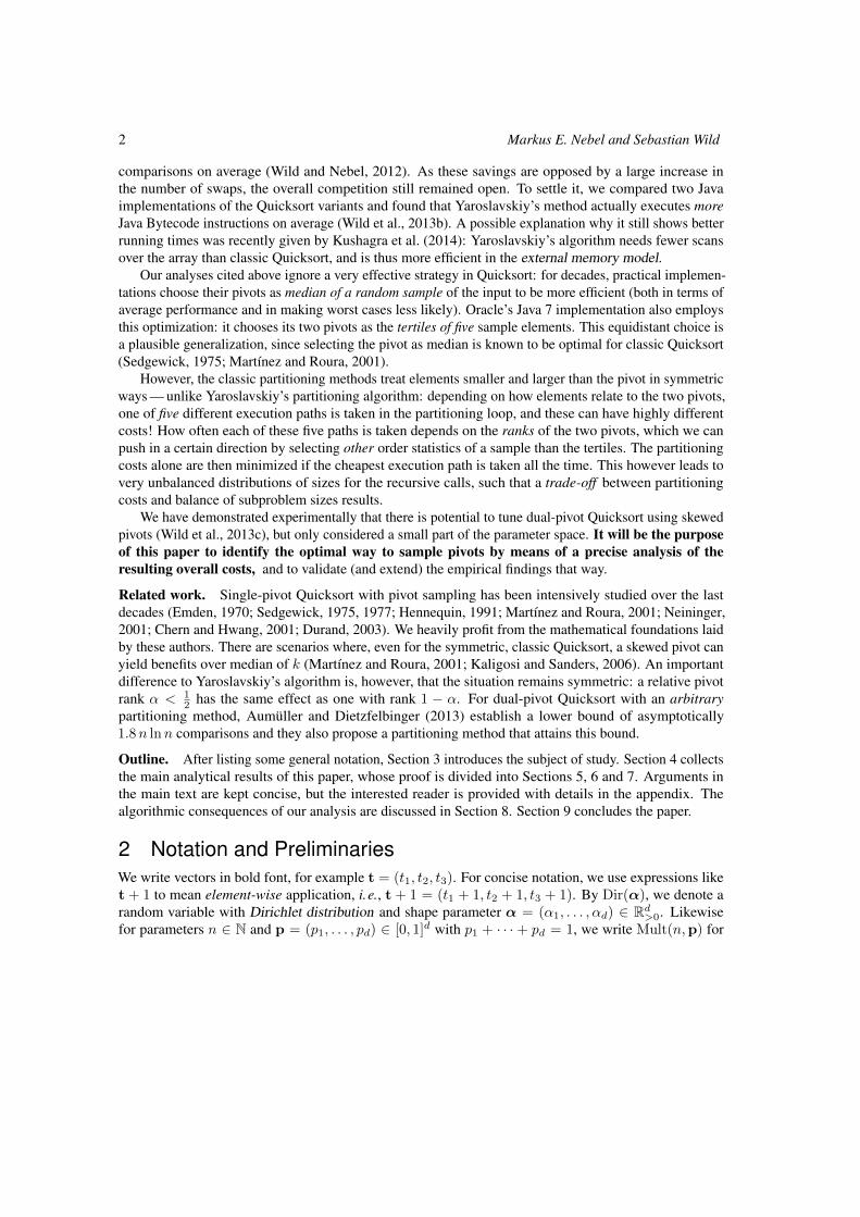
0 1P Q
D1 D2 D3
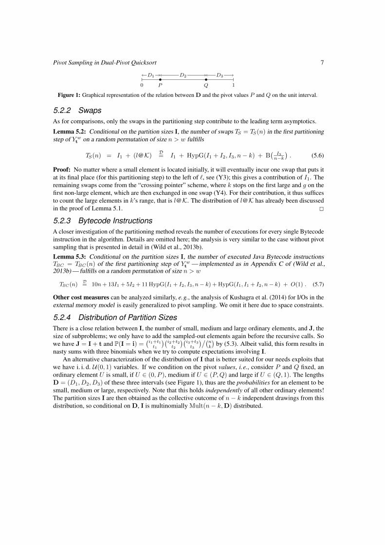
Figure 1: Graphical representation of the relation between D and the pivot values P and Q on the unit interval.
5.2.2 SwapsAs for comparisons, only the swaps in the partitioning step contribute to the leading term asymptotics.
Lemma 5.2: Conditional on the partition sizes I, the number of swaps TS = TS(n) in the first partitioningstep of Y wt on a random permutation of size n > w fulfills
TS(n) = I1 + (l@K)D= I1 + HypG(I1 + I2, I3, n− k) + B
(I3n−k
). (5.6)
Proof: No matter where a small element is located initially, it will eventually incur one swap that puts itat its final place (for this partitioning step) to the left of `, see (Y3); this gives a contribution of I1. Theremaining swaps come from the “crossing pointer” scheme, where k stops on the first large and g on thefirst non-large element, which are then exchanged in one swap (Y4). For their contribution, it thus sufficesto count the large elements in k’s range, that is l@K. The distribution of l@K has already been discussedin the proof of Lemma 5.1. 2
5.2.3 Bytecode InstructionsA closer investigation of the partitioning method reveals the number of executions for every single Bytecodeinstruction in the algorithm. Details are omitted here; the analysis is very similar to the case without pivotsampling that is presented in detail in (Wild et al., 2013b).Lemma 5.3: Conditional on the partition sizes I, the number of executed Java Bytecode instructionsTBC = TBC (n) of the first partitioning step of Y wt — implemented as in Appendix C of (Wild et al.,2013b) — fulfills on a random permutation of size n > w
TBC (n)D= 10n+ 13I1 + 5I2 + 11HypG(I1 + I2, I3, n− k) +HypG(I1, I1 + I2, n− k) + O(1) . (5.7)
Other cost measures can be analyzed similarly, e.g., the analysis of Kushagra et al. (2014) for I/Os in theexternal memory model is easily generalized to pivot sampling. We omit it here due to space constraints.
5.2.4 Distribution of Partition SizesThere is a close relation between I, the number of small, medium and large ordinary elements, and J, thesize of subproblems; we only have to add the sampled-out elements again before the recursive calls. Sowe have J = I + t and P(I = i) =
(i1+t1t1
)(i2+t2t2
)(i3+t3t3
)/(nk
)by (5.3). Albeit valid, this form results in
nasty sums with three binomials when we try to compute expectations involving I.An alternative characterization of the distribution of I that is better suited for our needs exploits that
we have i. i. d. U(0, 1) variables. If we condition on the pivot values, i.e., consider P and Q fixed, anordinary element U is small, if U ∈ (0, P ), medium if U ∈ (P,Q) and large if U ∈ (Q, 1). The lengthsD = (D1, D2, D3) of these three intervals (see Figure 1), thus are the probabilities for an element to besmall, medium or large, respectively. Note that this holds independently of all other ordinary elements!The partition sizes I are then obtained as the collective outcome of n− k independent drawings from thisdistribution, so conditional on D, I is multinomially Mult(n− k,D) distributed.
8 Markus E. Nebel and Sebastian Wild
With this alternative characterization, we have decoupled the pivot ranks (determined by I) from thepivot values, which allows for a more elegant computation of expected values (see Appendix D). Thisdecoupling trick has (implicitly) been applied to the analysis of classic Quicksort earlier, e.g., by Neininger(2001).
5.2.5 Distribution of Pivot ValuesThe input array is initially filled with n i. i. d. U(0, 1) random variables from which we choose a sample{V1, . . . , Vk} ⊂ {U1, . . . , Un} of size k. The pivot values are then selected as order statistics of the sample:P := V(t1+1) and Q := V(t1+t2+2) (cf. Section 3.1). In other words, D is the vector of spacings inducedby the order statistics V(t1+1) and V(t1+t2+2) of k i. i. d. U(0, 1) variables V1, . . . , Vk, which is known tohave a Dirichlet Dir(t + 1) distribution (Proposition C.1 in the appendix).
6 Expected Partitioning CostsIn Section 5, we characterized the full distribution of the costs of the first partitioning step. However, sincethose distributions are conditional on other random variables, we have to apply the law of total expectation.By linearity of the expectation, it suffices to consider the following summands:Lemma 6.1: For pivot sampling parameter t ∈ N3 and partition sizes I D= Mult(n − k,D), based onrandom spacings D D= Dir(t + 1), the following (unconditional) expectations hold:
E[Ij ] =tj + 1
k + 1(n− k) , (j = 1, 2, 3), (6.1)
E[B(I3n−k
)]=
t3 + 1
k + 1= Θ(1) , (n→∞), (6.2)
E[HypG(I3, I1, n− k)
]=
(t1 + 1)(t3 + 1)
(k + 1)(k + 2)(n− k − 1) , (6.3)
E[HypG(I1 + I2, I3, n− k)
]=
(t1 + t2 + 2)(t3 + 1)
(k + 1)(k + 2)(n− k − 1) . (6.4)
Using known properties of the involved distributions, the proof is elementary; see Appendix D for details.
7 Solution of the RecurrenceTheorem 7.1: Let E[Cn] be a sequence of numbers satisfying recurrence (5.2) on page 5 for a constantw ≥ k and let the toll function E[Tn] be of the form E[Tn] = an+O(1) for a constant a. Then we haveE[Cn] ∼ a
H(t) n lnn, where H(t) is given by equation (4.1) on page 4.
Theorem 7.1 has first been proven by Hennequin (1991, Proposition III.9) using arguments on theCauchy-Euler differential equations that the recurrence implies for the generating function of E[Cn]. Thetool box of handy and ready-to-apply theorems has grown considerably since then. In Appendix E, wegive a concise and elementary proof using the Continuous Master Theorem (Roura, 2001): we showthat the distribution of the relative subproblem sizes converges to a Beta distribution and that then acontinuous version of the recursion tree argument allows to solve our recurrence. An alternative tool closerto Hennequin’s original arguments is offered by Chern et al. (2002).
Theorem 4.1 now directly follows by using Lemma 6.1 on the partitioning costs from Lemma 5.1, 5.2and 5.3 and plugging the result into Theorem 7.1.
Pivot Sampling in Dual-Pivot Quicksort 9
+68.7%−17.7%
+38.9%
+32.5%−8.84%
+20.8%
+18.8%−1.36%
+17.2%
+15.0%+4.76%+20.4%
+18.8%+9.52%+30.1%
+32.5%+12.9%+49.7%
+68.7%+15.0%+94.0%
+32.5%−11.6%
+17.2%
+11.4%−4.76%
+6.09%
+3.86%+0.680%+4.57%
+3.86%+4.76%+8.81%
+11.4%+7.48%+19.7%
+32.5%+8.84%+44.3%
+18.8%−8.16%
+9.08%
+3.86%−3.40%
+0.331%
+3.86%+2.04%+5.98%
+18.8%+2.72%+22.0%
+15.0%−7.48%
+6.37%
+3.86%−4.76%−1.08%
+3.86%−3.40%
+0.331%
+15.0%−3.40%
+11.1%
+18.8%−9.52%
+7.47%
+11.4%−8.84%
+1.54%
+18.8%−9.52%
+7.47%
+32.5%−14.3%
+13.6%
+32.5%−15.6%
+11.8%
+68.7%−21.8%
+32.0%
t1 = 0
t2 = 0
t1 = 1
t2 = 1
t1 = 2
t2 = 2
t1 = 3
t2 = 3
t1 = 4
t2 = 4
t1 = 5
t2 = 5
t1 = 6
t2 = 6
1/H(t):aC :
aC/H(t):
+15.0%−7.48%
+6.37%
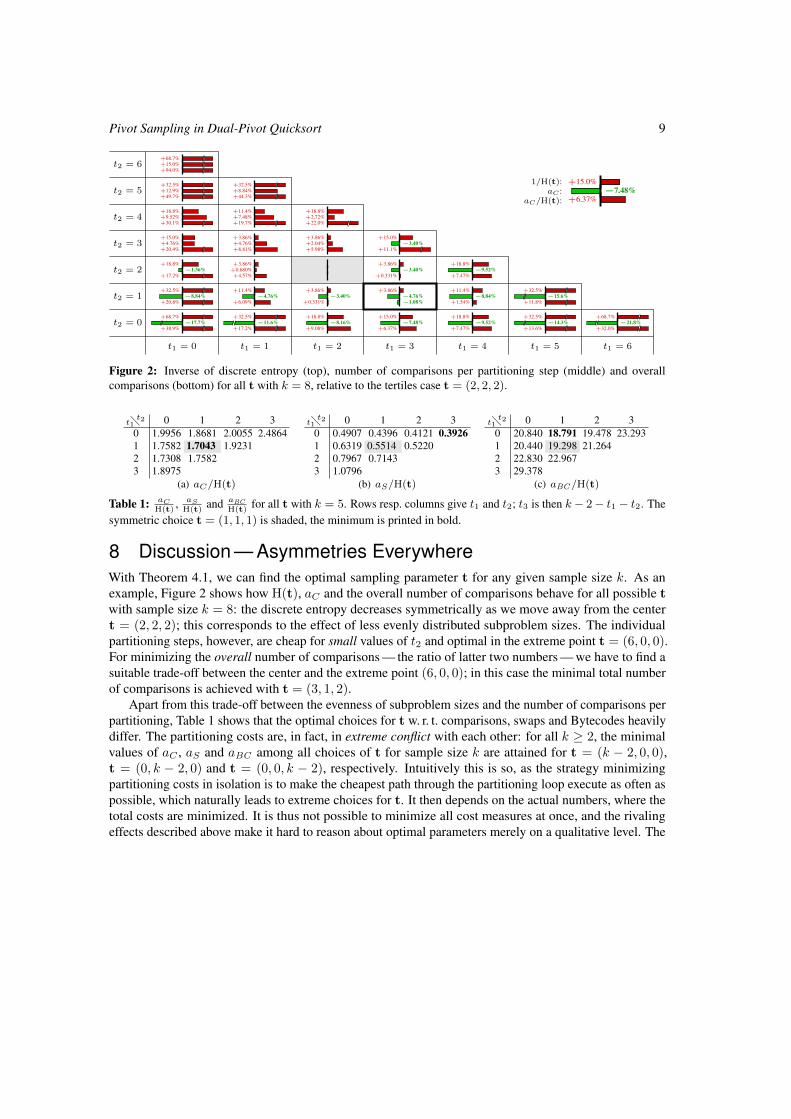
Figure 2: Inverse of discrete entropy (top), number of comparisons per partitioning step (middle) and overallcomparisons (bottom) for all t with k = 8, relative to the tertiles case t = (2, 2, 2).
t1�t2 0 1 2 30 1.9956 1.8681 2.0055 2.48641 1.7582 1.7043 1.92312 1.7308 1.75823 1.8975
(a) aC/H(t)
t1�t2 0 1 2 30 0.4907 0.4396 0.4121 0.39261 0.6319 0.5514 0.52202 0.7967 0.71433 1.0796
(b) aS/H(t)
t1�t2 0 1 2 30 20.840 18.791 19.478 23.2931 20.440 19.298 21.2642 22.830 22.9673 29.378
(c) aBC /H(t)
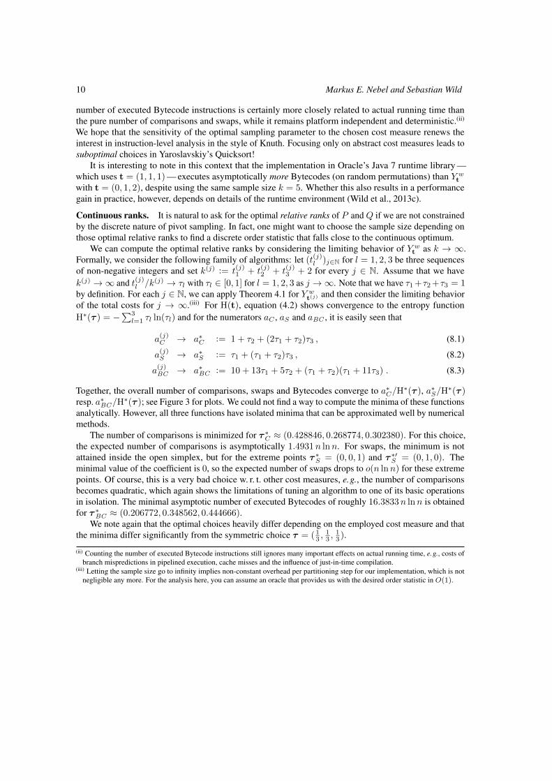
Table 1: aCH(t)
, aSH(t)
and aBCH(t)
for all t with k = 5. Rows resp. columns give t1 and t2; t3 is then k− 2− t1 − t2. Thesymmetric choice t = (1, 1, 1) is shaded, the minimum is printed in bold.
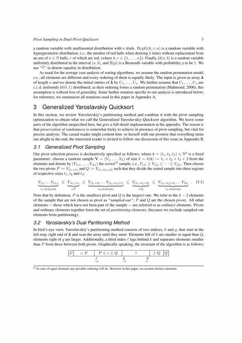
8 Discussion — Asymmetries EverywhereWith Theorem 4.1, we can find the optimal sampling parameter t for any given sample size k. As anexample, Figure 2 shows how H(t), aC and the overall number of comparisons behave for all possible twith sample size k = 8: the discrete entropy decreases symmetrically as we move away from the centert = (2, 2, 2); this corresponds to the effect of less evenly distributed subproblem sizes. The individualpartitioning steps, however, are cheap for small values of t2 and optimal in the extreme point t = (6, 0, 0).For minimizing the overall number of comparisons — the ratio of latter two numbers — we have to find asuitable trade-off between the center and the extreme point (6, 0, 0); in this case the minimal total numberof comparisons is achieved with t = (3, 1, 2).
Apart from this trade-off between the evenness of subproblem sizes and the number of comparisons perpartitioning, Table 1 shows that the optimal choices for t w. r. t. comparisons, swaps and Bytecodes heavilydiffer. The partitioning costs are, in fact, in extreme conflict with each other: for all k ≥ 2, the minimalvalues of aC , aS and aBC among all choices of t for sample size k are attained for t = (k − 2, 0, 0),t = (0, k − 2, 0) and t = (0, 0, k − 2), respectively. Intuitively this is so, as the strategy minimizingpartitioning costs in isolation is to make the cheapest path through the partitioning loop execute as often aspossible, which naturally leads to extreme choices for t. It then depends on the actual numbers, where thetotal costs are minimized. It is thus not possible to minimize all cost measures at once, and the rivalingeffects described above make it hard to reason about optimal parameters merely on a qualitative level. The
10 Markus E. Nebel and Sebastian Wild
number of executed Bytecode instructions is certainly more closely related to actual running time thanthe pure number of comparisons and swaps, while it remains platform independent and deterministic.(ii)
We hope that the sensitivity of the optimal sampling parameter to the chosen cost measure renews theinterest in instruction-level analysis in the style of Knuth. Focusing only on abstract cost measures leads tosuboptimal choices in Yaroslavskiy’s Quicksort!
It is interesting to note in this context that the implementation in Oracle’s Java 7 runtime library —which uses t = (1, 1, 1) — executes asymptotically more Bytecodes (on random permutations) than Y wtwith t = (0, 1, 2), despite using the same sample size k = 5. Whether this also results in a performancegain in practice, however, depends on details of the runtime environment (Wild et al., 2013c).
Continuous ranks. It is natural to ask for the optimal relative ranks of P and Q if we are not constrainedby the discrete nature of pivot sampling. In fact, one might want to choose the sample size depending onthose optimal relative ranks to find a discrete order statistic that falls close to the continuous optimum.
We can compute the optimal relative ranks by considering the limiting behavior of Y wt as k → ∞.Formally, we consider the following family of algorithms: let (t(j)l )j∈N for l = 1, 2, 3 be three sequencesof non-negative integers and set k(j) := t(j)1 + t(j)2 + t(j)3 + 2 for every j ∈ N. Assume that we havek(j) →∞ and t(j)l /k(j) → τl with τl ∈ [0, 1] for l = 1, 2, 3 as j →∞. Note that we have τ1 +τ2 +τ3 = 1by definition. For each j ∈ N, we can apply Theorem 4.1 for Y wt(j) and then consider the limiting behaviorof the total costs for j → ∞.(iii) For H(t), equation (4.2) shows convergence to the entropy functionH∗(τ ) = −
∑3l=1 τl ln(τl) and for the numerators aC , aS and aBC , it is easily seen that
a(j)C → a∗C := 1 + τ2 + (2τ1 + τ2)τ3 , (8.1)
a(j)S → a∗S := τ1 + (τ1 + τ2)τ3 , (8.2)
a(j)BC → a∗BC := 10 + 13τ1 + 5τ2 + (τ1 + τ2)(τ1 + 11τ3) . (8.3)
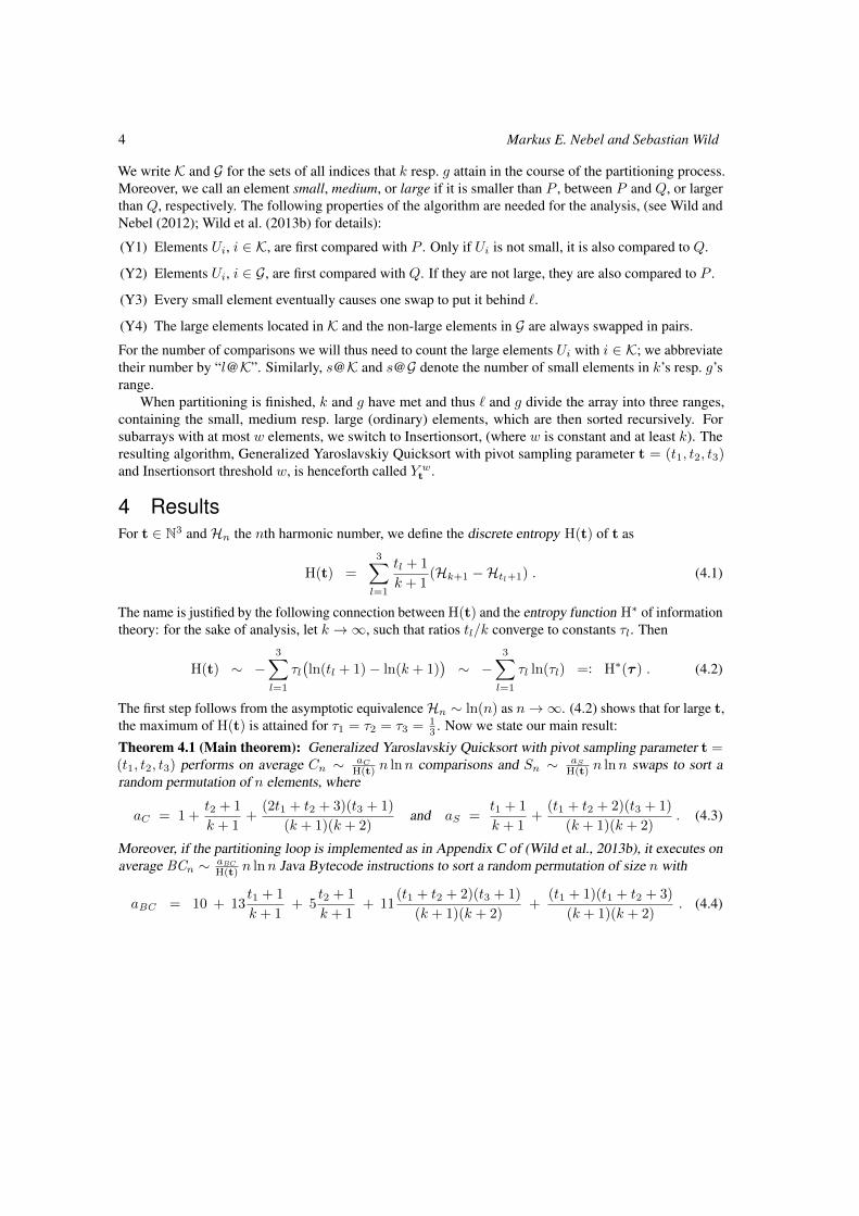
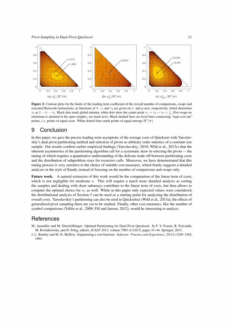
Together, the overall number of comparisons, swaps and Bytecodes converge to a∗C/H∗(τ ), a∗S/H
∗(τ )resp. a∗BC/H
∗(τ ); see Figure 3 for plots. We could not find a way to compute the minima of these functionsanalytically. However, all three functions have isolated minima that can be approximated well by numericalmethods.
The number of comparisons is minimized for τ ∗C ≈ (0.428846, 0.268774, 0.302380). For this choice,the expected number of comparisons is asymptotically 1.4931n lnn. For swaps, the minimum is notattained inside the open simplex, but for the extreme points τ ∗S = (0, 0, 1) and τ ∗′S = (0, 1, 0). Theminimal value of the coefficient is 0, so the expected number of swaps drops to o(n lnn) for these extremepoints. Of course, this is a very bad choice w. r. t. other cost measures, e.g., the number of comparisonsbecomes quadratic, which again shows the limitations of tuning an algorithm to one of its basic operationsin isolation. The minimal asymptotic number of executed Bytecodes of roughly 16.3833n lnn is obtainedfor τ ∗BC ≈ (0.206772, 0.348562, 0.444666).
We note again that the optimal choices heavily differ depending on the employed cost measure and thatthe minima differ significantly from the symmetric choice τ = ( 1
3 ,13 ,
13 ).
(ii) Counting the number of executed Bytecode instructions still ignores many important effects on actual running time, e.g., costs ofbranch mispredictions in pipelined execution, cache misses and the influence of just-in-time compilation.
(iii) Letting the sample size go to infinity implies non-constant overhead per partitioning step for our implementation, which is notnegligible any more. For the analysis here, you can assume an oracle that provides us with the desired order statistic in O(1).
Pivot Sampling in Dual-Pivot Quicksort 11
0 0.2 0.4 0.6 0.8 1
0
0.2
0.4
0.6
0.8
1
1.4931
1.5171
(a) a∗C/H∗(τ )
0 0.2 0.4 0.6 0.8 1
0
0.2
0.4
0.6
0.8
1
0.5057
(b) a∗S/H∗(τ )
0 0.2 0.4 0.6 0.8 1
0
0.2
0.4
0.6
0.8
1
16.383
16.991
(c) a∗BC /H∗(τ )
Figure 3: Contour plots for the limits of the leading term coefficient of the overall number of comparisons, swaps andexecuted Bytecode instructions, as functions of τ . τ1 and τ2 are given on x- and y-axis, respectively, which determineτ3 as 1− τ1− τ2. Black dots mark global minima, white dots show the center point τ1 = τ2 = τ3 = 1
3. (For swaps no
minimum is attained in the open simplex, see main text). Black dashed lines are level lines connecting “equi-cost-ant”points, i.e. points of equal costs. White dotted lines mark points of equal entropy H∗(τ ).
9 ConclusionIn this paper, we gave the precise leading term asymptotic of the average costs of Quicksort with Yaroslav-skiy’s dual-pivot partitioning method and selection of pivots as arbitrary order statistics of a constant sizesample. Our results confirm earlier empirical findings (Yaroslavskiy, 2010; Wild et al., 2013c) that theinherent asymmetries of the partitioning algorithm call for a systematic skew in selecting the pivots — thetuning of which requires a quantitative understanding of the delicate trade-off between partitioning costsand the distribution of subproblem sizes for recursive calls. Moreover, we have demonstrated that thistuning process is very sensitive to the choice of suitable cost measures, which firmly suggests a detailedanalyses in the style of Knuth, instead of focusing on the number of comparisons and swaps only.
Future work. A natural extension of this work would be the computation of the linear term of costs,which is not negligible for moderate n. This will require a much more detailed analysis as sortingthe samples and dealing with short subarrays contribute to the linear term of costs, but then allows tocompute the optimal choice for w, as well. While in this paper only expected values were considered,the distributional analysis of Section 5 can be used as a starting point for analyzing the distribution ofoverall costs. Yaroslavskiy’s partitioning can also be used in Quickselect (Wild et al., 2013a); the effects ofgeneralized pivot sampling there are yet to be studied. Finally, other cost measures, like the number ofsymbol comparisons (Vallée et al., 2009; Fill and Janson, 2012), would be interesting to analyze.
ReferencesM. Aumüller and M. Dietzfelbinger. Optimal Partitioning for Dual Pivot Quicksort. In F. V. Fomin, R. Freivalds,
M. Kwiatkowska, and D. Peleg, editors, ICALP 2013, volume 7965 of LNCS, pages 33–44. Springer, 2013.J. L. Bentley and M. D. McIlroy. Engineering a sort function. Software: Practice and Experience, 23(11):1249–1265,
1993.
12 Markus E. Nebel and Sebastian Wild
H.-H. Chern and H.-K. Hwang. Transitional behaviors of the average cost of quicksort with median-of-(2t + 1).Algorithmica, 29(1-2):44–69, 2001.
H.-H. Chern, H.-K. Hwang, and T.-H. Tsai. An asymptotic theory for Cauchy–Euler differential equations withapplications to the analysis of algorithms. Journal of Algorithms, 44(1):177–225, 2002.
H. A. David and H. N. Nagaraja. Order Statistics (Wiley Series in Probability and Statistics). Wiley-Interscience, 3rdedition, 2003. ISBN 0-471-38926-9.
M. Durand. Asymptotic analysis of an optimized quicksort algorithm. Information Processing Letters, 85(2):73–77,2003.
M. H. v. Emden. Increasing the efficiency of quicksort. Communications of the ACM, pages 563–567, 1970.V. Estivill-Castro and D. Wood. A survey of adaptive sorting algorithms. ACM Computing Surveys, 24(4):441–476,
1992.J. Fill and S. Janson. The number of bit comparisons used by Quicksort: an average-case analysis. Electronic Journal
of Probability, 17:1–22, 2012.R. L. Graham, D. E. Knuth, and O. Patashnik. Concrete mathematics: a foundation for computer science. Addison-
Wesley, 1994. ISBN 978-0-20-155802-9.P. Hennequin. Analyse en moyenne d’algorithmes : tri rapide et arbres de recherche. PhD Thesis, Ecole Politechnique,
Palaiseau, 1991.C. A. R. Hoare. Algorithm 65: Find. Communications of the ACM, 4(7):321–322, July 1961.K. Kaligosi and P. Sanders. How branch mispredictions affect quicksort. In T. Erlebach and Y. Azar, editors, ESA
2006, pages 780–791. Springer, 2006.S. Kushagra, A. López-Ortiz, A. Qiao, and J. I. Munro. Multi-Pivot Quicksort: Theory and Experiments. In ALENEX
2014, pages 47–60. SIAM, 2014.H. M. Mahmoud. Sorting: A distribution theory. John Wiley & Sons, Hoboken, NJ, USA, 2000. ISBN 1-118-03288-8.C. Martínez and S. Roura. Optimal Sampling Strategies in Quicksort and Quickselect. SIAM Journal on Computing,
31(3):683, 2001.D. R. Musser. Introspective Sorting and Selection Algorithms. Software: Practice and Experience, 27(8):983–993,
1997.R. Neininger. On a multivariate contraction method for random recursive structures with applications to Quicksort.
Random Structures & Algorithms, 19(3-4):498–524, 2001.S. Roura. Improved Master Theorems for Divide-and-Conquer Recurrences. Journal of the ACM, 48(2):170–205,
2001.R. Sedgewick. Quicksort. PhD Thesis, Stanford University, 1975.R. Sedgewick. The analysis of Quicksort programs. Acta Inf., 7(4):327–355, 1977.R. Sedgewick. Implementing Quicksort programs. Communications of the ACM, 21(10):847–857, 1978.B. Vallée, J. Clément, J. A. Fill, and P. Flajolet. The Number of Symbol Comparisons in QuickSort and QuickSelect.
In S. Albers, A. Marchetti-Spaccamela, Y. Matias, S. Nikoletseas, and W. Thomas, editors, ICALP 2009, volume5555 of LNCS, pages 750–763. Springer, 2009.
S. Wild and M. E. Nebel. Average Case Analysis of Java 7’s Dual Pivot Quicksort. In L. Epstein and P. Ferragina,editors, ESA 2012, volume 7501 of LNCS, pages 825–836. Springer, 2012.
S. Wild, M. E. Nebel, and H. Mahmoud. Analysis of Quickselect under Yaroslavskiy’s Dual-Pivoting Algorithm,2013a. URL http://arxiv.org/abs/1306.3819.
S. Wild, M. E. Nebel, and R. Neininger. Average Case and Distributional Analysis of Java 7’s Dual Pivot Quicksort,2013b. URL http://arxiv.org/abs/1304.0988.
S. Wild, M. E. Nebel, R. Reitzig, and U. Laube. Engineering Java 7’s Dual Pivot Quicksort Using MaLiJAn. InP. Sanders and N. Zeh, editors, ALENEX 2013, pages 55–69. SIAM, 2013c.
V. Yaroslavskiy. Question on sorting. http://mail.openjdk.java.net/pipermail/core-libs-dev/2010-July/004649.html, 2010.
Pivot Sampling in Dual-Pivot Quicksort 13
Appendix
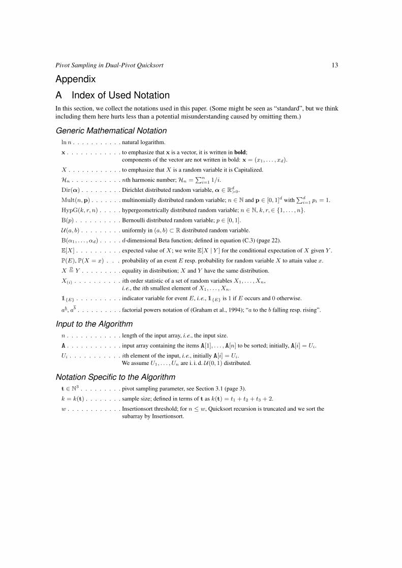
A Index of Used NotationIn this section, we collect the notations used in this paper. (Some might be seen as “standard”, but we thinkincluding them here hurts less than a potential misunderstanding caused by omitting them.)
Generic Mathematical Notationlnn . . . . . . . . . . . natural logarithm.
x . . . . . . . . . . . . to emphasize that x is a vector, it is written in bold;components of the vector are not written in bold: x = (x1, . . . , xd).
X . . . . . . . . . . . . to emphasize that X is a random variable it is Capitalized.
Hn . . . . . . . . . . . nth harmonic number;Hn =∑n
i=1 1/i.
Dir(α) . . . . . . . . . Dirichlet distributed random variable, α ∈ Rd>0.
Mult(n,p) . . . . . . . multinomially distributed random variable; n ∈ N and p ∈ [0, 1]d with∑d
i=1 pi = 1.
HypG(k, r, n) . . . . . hypergeometrically distributed random variable; n ∈ N, k, r,∈ {1, . . . , n}.B(p) . . . . . . . . . . Bernoulli distributed random variable; p ∈ [0, 1].
U(a, b) . . . . . . . . . uniformly in (a, b) ⊂ R distributed random variable.
B(α1, . . . , αd) . . . . . d-dimensional Beta function; defined in equation (C.3) (page 22).
E[X] . . . . . . . . . . expected value of X; we write E[X | Y ] for the conditional expectation of X given Y .
P(E), P(X = x) . . . probability of an event E resp. probability for random variable X to attain value x.
X D= Y . . . . . . . . . equality in distribution; X and Y have the same distribution.
X(i) . . . . . . . . . . ith order statistic of a set of random variables X1, . . . , Xn,i.e., the ith smallest element of X1, . . . , Xn.
1{E} . . . . . . . . . . indicator variable for event E, i.e., 1{E} is 1 if E occurs and 0 otherwise.
ab, ab . . . . . . . . . . factorial powers notation of (Graham et al., 1994); “a to the b falling resp. rising”.
Input to the Algorithmn . . . . . . . . . . . . length of the input array, i.e., the input size.
A . . . . . . . . . . . . input array containing the items A[1], . . . ,A[n] to be sorted; initially, A[i] = Ui.
Ui . . . . . . . . . . . ith element of the input, i.e., initially A[i] = Ui.We assume U1, . . . , Un are i. i. d. U(0, 1) distributed.
Notation Specific to the Algorithmt ∈ N3 . . . . . . . . . pivot sampling parameter, see Section 3.1 (page 3).
k = k(t) . . . . . . . . sample size; defined in terms of t as k(t) = t1 + t2 + t3 + 2.
w . . . . . . . . . . . . Insertionsort threshold; for n ≤ w, Quicksort recursion is truncated and we sort thesubarray by Insertionsort.
14 Markus E. Nebel and Sebastian Wild
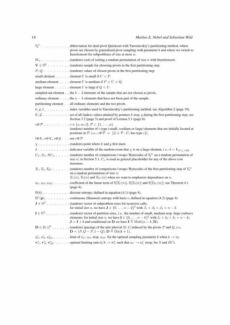
Y wt . . . . . . . . . . . abbreviation for dual-pivot Quicksort with Yaroslavskiy’s partitioning method, where
pivots are chosen by generalized pivot sampling with parameter t and where we switch toInsertionsort for subproblems of size at most w.
Wn . . . . . . . . . . . (random) costs of sorting a random permutation of size n with Insertionsort.
V ∈ Nk . . . . . . . . (random) sample for choosing pivots in the first partitioning step.
P , Q . . . . . . . . . . (random) values of chosen pivots in the first partitioning step.
small element . . . . . element U is small if U < P .
medium element . . . . element U is medium if P < U < Q.
large element . . . . . . element U is large if Q < U .
sampled-out element . . the k − 2 elements of the sample that are not chosen as pivots.
ordinary element . . . . the n− k elements that have not been part of the sample.
partitioning element . . all ordinary elements and the two pivots.
k, g, ` . . . . . . . . . index variables used in Yaroslavskiy’s partitioning method, see Algorithm 2 (page 19).
K, G . . . . . . . . . . set of all (index) values attained by pointers k resp. g during the first partitioning step; seeSection 3.2 (page 3) and proof of Lemma 5.1 (page 6).
c@P . . . . . . . . . . c ∈ {s,m, l}, P ⊂ {1, . . . , n}(random) number of c-type (small, medium or large) elements that are initially located atpositions in P , i.e., c@P =
∣∣{i ∈ P : Ui has type c}∣∣.
l@K, s@K, s@G . . . see c@Pχ . . . . . . . . . . . . (random) point where k and g first meet.
δ . . . . . . . . . . . . indicator variable of the random event that χ is on a large element, i.e., δ = 1{Uχ>Q}.
Cn, Sn, BCn . . . . . (random) number of comparisons / swaps / Bytecodes of Y wt on a random permutation of
size n; in Section 5.1, Cn is used as general placeholder for any of the above costmeasures.
TC , TS , TBC . . . . . . (random) number of comparisons / swaps / Bytecodes of the first partitioning step of Y wt
on a random permutation of size n;TC(n), TS(n) and TBC (n) when we want to emphasize dependence on n.
aC , aS , aBC . . . . . . coefficient of the linear term of E[TC(n)], E[TS(n)] and E[TBC (n)]; see Theorem 4.1(page 4).
H(t) . . . . . . . . . . discrete entropy; defined in equation (4.1) (page 4).
H∗(p) . . . . . . . . . continuous (Shannon) entropy with basis e; defined in equation (4.2) (page 4).
J ∈ N3 . . . . . . . . . (random) vector of subproblem sizes for recursive calls;for initial size n, we have J ∈ {0, . . . , n− 2}3 with J1 + J2 + J3 = n− 2.
I ∈ N3 . . . . . . . . . (random) vector of partition sizes, i.e., the number of small, medium resp. large ordinaryelements; for initial size n, we have I ∈ {0, . . . , n− k}3 with I1 + I2 + I3 = n− k;J = I+ t and conditional on D we have I D= Mult(n− k,D).
D ∈ [0, 1]3 . . . . . . . (random) spacings of the unit interval (0, 1) induced by the pivots P and Q, i.e.,D = (P,Q− P, 1−Q); D D= Dir(t+ 1).
a∗C , a∗S , a∗BC . . . . . . limit of aC , aS , resp. aBC for the optimal sampling parameter t when k →∞.
τ ∗C , τ ∗S , τ ∗BC . . . . . optimal limiting ratio t/k → τ ∗C such that aC → a∗C (resp. for S and BC ).
Pivot Sampling in Dual-Pivot Quicksort 15
B Detailed PseudocodeB.1 Implementing Generalized Pivot SamplingWhile extensive literature on the analysis of (single-pivot) Quicksort with pivot sampling is available, mostworks do not specify the pivot selection process in detail.(iv) The usual justification is that, in any case,we only draw pivots a linear number of times and from a constant size sample. So for the leading termasymptotic, the costs of pivot selection are negligible, and hence also the precise way of how selection isdone is not important.
There is one caveat in the argumentation: Analyses of Quicksort usually rely on setting up a recurrenceequation of expected costs that is then solved (precisely or asymptotically). This in turn requires thealgorithm to preserve the distribution of input permutations for the subproblems subjected to recursivecalls — otherwise the recurrence does not hold. Most partitioning algorithms, including the one ofYaroslavskiy, have the desirable property to preserve randomness (Wild and Nebel, 2012); but this is notsufficient! We also have to make sure that the main procedure of Quicksort does not alter the distribution ofinputs for recursive calls; in connection with elaborate pivot sampling algorithms, this is harder to achievethan it might seem at first sight.
For these reasons, the authors felt the urge to include a minute discussion of how to implement thegeneralized pivot sampling scheme of Section 3.1 in such a way that the recurrence equation remainsprecise.(v) We have to address the following questions:
Which elements do we choose for the sample? In theory, a random sample produces the most reliableresults and also protects against worst case inputs. The use of a random pivot for classic Quicksort hasbeen considered right from its invention (Hoare, 1961) and is suggested as a general strategy to deal withbiased data (Sedgewick, 1978).
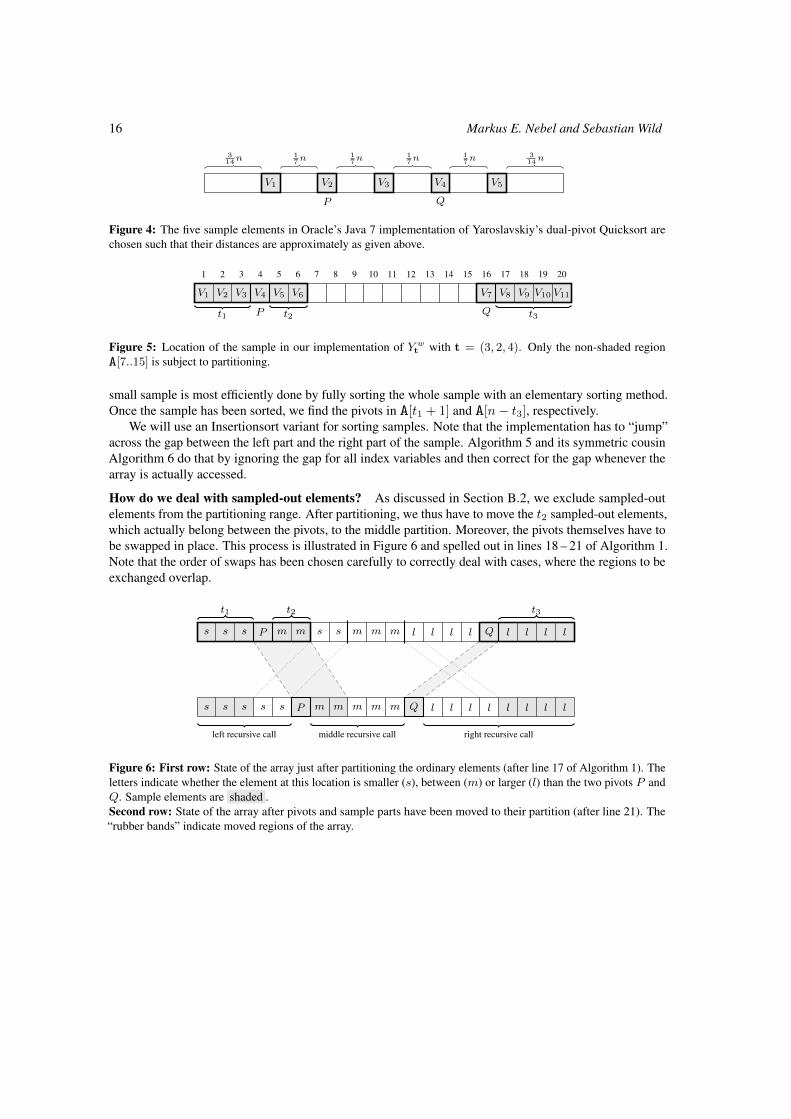
However, all programming libraries known to the authors actually avoid the additional effort of drawingrandom samples. They use a set of deterministically selected positions of the array, instead; chosen to givereasonable results for common special cases like almost sorted arrays. For example, the positions used inOracle’s Java 7 implementation are depicted in Figure 4.
For our analysis, the input consists of i. i. d. random variables, so all subsets (of a certain size) have thesame distribution. We might hence select the positions of sample elements such that they are convenientfor our (analysis) purposes. For reasons elaborated in Section B.2 below, we have to exclude sampled-outelements from partitioning to keep analysis feasible, and therefore, our implementation uses the t1 + t2 + 1leftmost and the t3 + 1 rightmost elements of the array as sample, as illustrated in Figure 5. Then,partitioning can be simply restricted to the range between the two parts of the sample, namely positionst1 + t2 + 2 through n− t3 − 1.
How do we select the desired order statistics from the sample? Finding a given order statistic of a listof elements is known as the selection problem and can be solved by specialized algorithms like Quickselect.Even though these selection algorithms are superior by far on large lists, selecting pivots from a reasonably
(iv) Noteworthy exceptions are Sedgewick’s seminal works which give detailed code for the median-of-three strategy (Sedgewick,1975, 1978) and Bentley and McIlroy’s influential paper on engineering a practical sorting method (Bentley and McIlroy, 1993).Martínez and Roura describe a general approach of which they state that randomness is not preserved, but in their analysis, they“disregard the small amount of sortedness [ . . . ] yielding at least a good approximation” (Martínez and Roura, 2001, Section 7.2).
(v) Note that the resulting implementation has to be considered “academic”: While it is well-suited for precise analysis, it will looksomewhat peculiar from a practical point of view and productive use is probably not to be recommended.
16 Markus E. Nebel and Sebastian Wild
314n
17n
17n
17n
17n
314n
P Q
V1 V2 V3 V4 V5
Figure 4: The five sample elements in Oracle’s Java 7 implementation of Yaroslavskiy’s dual-pivot Quicksort arechosen such that their distances are approximately as given above.
1 2 3 4 5 6 7 8 9 10 11 12 13 14 15 16 17 18 19 20
t1 t2 t3P Q
V1 V2 V3 V4 V5 V6 V7 V8 V9 V10 V11
Figure 5: Location of the sample in our implementation of Y wt with t = (3, 2, 4). Only the non-shaded region
A[7..15] is subject to partitioning.
small sample is most efficiently done by fully sorting the whole sample with an elementary sorting method.Once the sample has been sorted, we find the pivots in A[t1 + 1] and A[n− t3], respectively.
We will use an Insertionsort variant for sorting samples. Note that the implementation has to “jump”across the gap between the left part and the right part of the sample. Algorithm 5 and its symmetric cousinAlgorithm 6 do that by ignoring the gap for all index variables and then correct for the gap whenever thearray is actually accessed.
How do we deal with sampled-out elements? As discussed in Section B.2, we exclude sampled-outelements from the partitioning range. After partitioning, we thus have to move the t2 sampled-out elements,which actually belong between the pivots, to the middle partition. Moreover, the pivots themselves have tobe swapped in place. This process is illustrated in Figure 6 and spelled out in lines 18 – 21 of Algorithm 1.Note that the order of swaps has been chosen carefully to correctly deal with cases, where the regions to beexchanged overlap.
t1 t2 t3
P Qs s s s sm m m m m l l l l l l l l
P Qs s s s s m m m m m l l l l l l l l
left recursive call middle recursive call right recursive call
Figure 6: First row: State of the array just after partitioning the ordinary elements (after line 17 of Algorithm 1). Theletters indicate whether the element at this location is smaller (s), between (m) or larger (l) than the two pivots P andQ. Sample elements are shaded .Second row: State of the array after pivots and sample parts have been moved to their partition (after line 21). The“rubber bands” indicate moved regions of the array.
Pivot Sampling in Dual-Pivot Quicksort 17
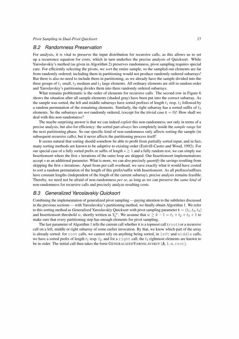
B.2 Randomness PreservationFor analysis, it is vital to preserve the input distribution for recursive calls, as this allows us to setup a recurrence equation for costs, which in turn underlies the precise analysis of Quicksort. WhileYaroslavskiy’s method (as given in Algorithm 2) preserves randomness, pivot sampling requires specialcare. For efficiently selecting the pivots, we sort the entire sample, so the sampled-out elements are farfrom randomly ordered; including them in partitioning would not produce randomly ordered subarrays!But there is also no need to include them in partitioning, as we already have the sample divided into thethree groups of t1 small, t2 medium and t3 large elements. All ordinary elements are still in random orderand Yaroslavskiy’s partitioning divides them into three randomly ordered subarrays.
What remains problematic is the order of elements for recursive calls. The second row in Figure 6shows the situation after all sample elements (shaded gray) have been put into the correct subarray. Asthe sample was sorted, the left and middle subarrays have sorted prefixes of length t1 resp. t2 followed bya random permutation of the remaining elements. Similarly, the right subarray has a sorted suffix of t3elements. So the subarrays are not randomly ordered, (except for the trivial case t = 0)! How shall wedeal with this non-randomness?
The maybe surprising answer is that we can indeed exploit this non-randomness; not only in terms of aprecise analysis, but also for efficiency: the sorted part always lies completely inside the sample range forthe next partitioning phase. So our specific kind of non-randomness only affects sorting the sample (insubsequent recursive calls), but it never affects the partitioning process itself!
It seems natural that sorting should somehow be able to profit from partially sorted input, and in fact,many sorting methods are known to be adaptive to existing order (Estivill-Castro and Wood, 1992). Forour special case of a fully sorted prefix or suffix of length s ≥ 1 and a fully random rest, we can simply useInsertionsort where the first s iterations of the outer loop are skipped. Our Insertionsort implementationsaccept s as an additional parameter. What is more, we can also precisely quantify the savings resulting fromskipping the first s iterations: Apart from per-call overhead, we save exactly what it would have costedto sort a random permutation of the length of this prefix/suffix with Insertionsort. As all prefixes/suffixeshave constant lengths (independent of the length of the current subarray), precise analysis remains feasible.Thereby, we need not be afraid of non-randomness per se, as long as we can preserve the same kind ofnon-randomness for recursive calls and precisely analyze resulting costs.
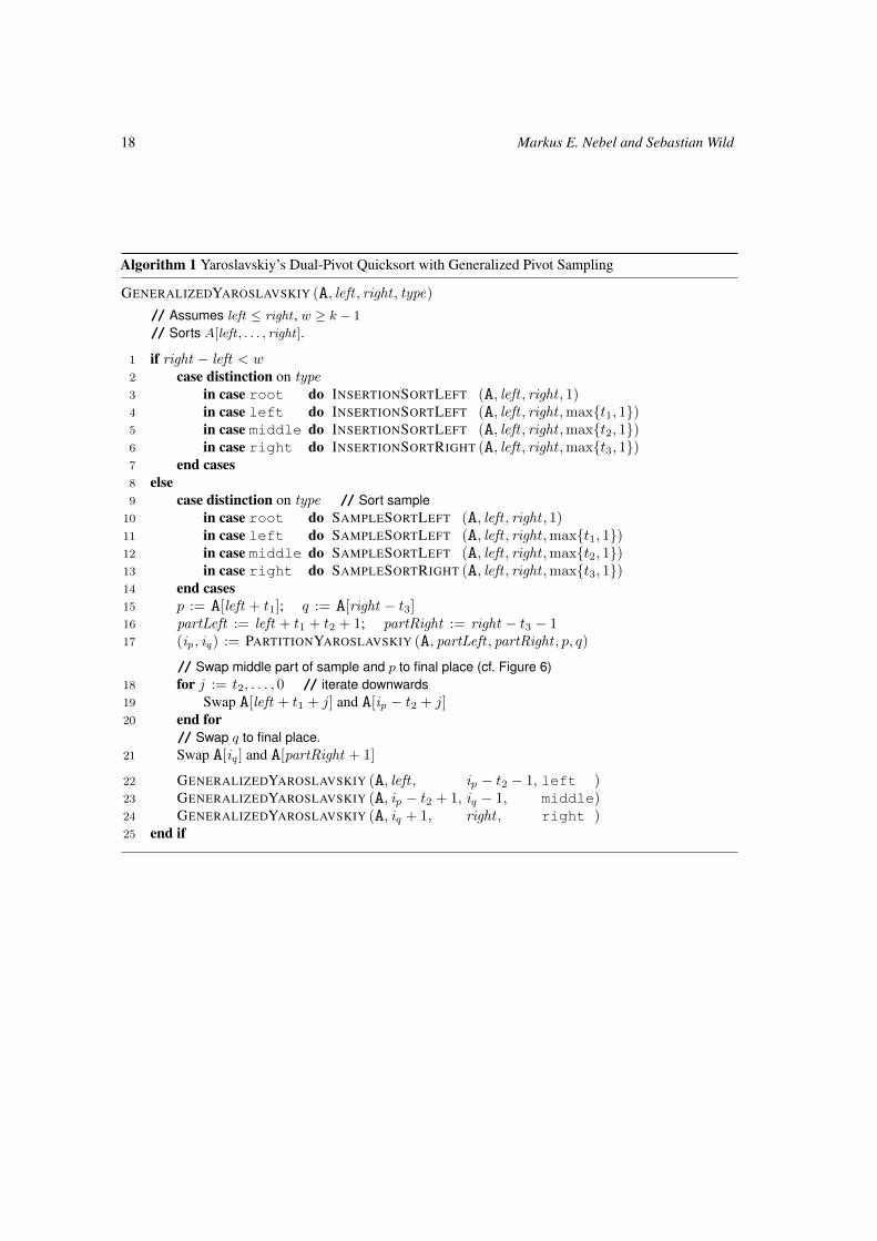
B.3 Generalized Yaroslavskiy QuicksortCombining the implementation of generalized pivot sampling — paying attention to the subtleties discussedin the previous sections — with Yaroslavskiy’s partitioning method, we finally obtain Algorithm 1. We referto this sorting method as Generalized Yaroslavskiy Quicksort with pivot sampling parameter t = (t1, t2, t3)and Insertionsort threshold w, shortly written as Y wt . We assume that w ≥ k − 1 = t1 + t2 + t3 + 1 tomake sure that every partitioning step has enough elements for pivot sampling.
The last parameter of Algorithm 1 tells the current call whether it is a topmost call (root) or a recursivecall on a left, middle or right subarray of some earlier invocation. By that, we know which part of the arrayis already sorted: for root calls, we cannot rely on anything being sorted, in left and middle calls,we have a sorted prefix of length t1 resp. t2, and for a right call, the t3 rightmost elements are known tobe in order. The initial call then takes the form GENERALIZEDYAROSLAVSKIY (A, 1, n,root).
18 Markus E. Nebel and Sebastian Wild
Algorithm 1 Yaroslavskiy’s Dual-Pivot Quicksort with Generalized Pivot Sampling
GENERALIZEDYAROSLAVSKIY (A, left , right , type)
// Assumes left ≤ right , w ≥ k − 1
// Sorts A[left , . . . , right ].
1 if right − left < w2 case distinction on type3 in case root do INSERTIONSORTLEFT (A, left , right , 1)4 in case left do INSERTIONSORTLEFT (A, left , right ,max{t1, 1})5 in case middle do INSERTIONSORTLEFT (A, left , right ,max{t2, 1})6 in case right do INSERTIONSORTRIGHT (A, left , right ,max{t3, 1})7 end cases8 else9 case distinction on type // Sort sample
10 in case root do SAMPLESORTLEFT (A, left , right , 1)11 in case left do SAMPLESORTLEFT (A, left , right ,max{t1, 1})12 in case middle do SAMPLESORTLEFT (A, left , right ,max{t2, 1})13 in case right do SAMPLESORTRIGHT (A, left , right ,max{t3, 1})14 end cases15 p := A[left + t1]; q := A[right − t3]16 partLeft := left + t1 + t2 + 1; partRight := right − t3 − 117 (ip , iq) := PARTITIONYAROSLAVSKIY (A, partLeft , partRight , p, q)
// Swap middle part of sample and p to final place (cf. Figure 6)18 for j := t2, . . . , 0 // iterate downwards19 Swap A[left + t1 + j] and A[ip − t2 + j]20 end for
// Swap q to final place.21 Swap A[iq ] and A[partRight + 1]
22 GENERALIZEDYAROSLAVSKIY (A, left , ip − t2 − 1, left )23 GENERALIZEDYAROSLAVSKIY (A, ip − t2 + 1, iq − 1, middle)24 GENERALIZEDYAROSLAVSKIY (A, iq + 1, right , right )25 end if
Pivot Sampling in Dual-Pivot Quicksort 19
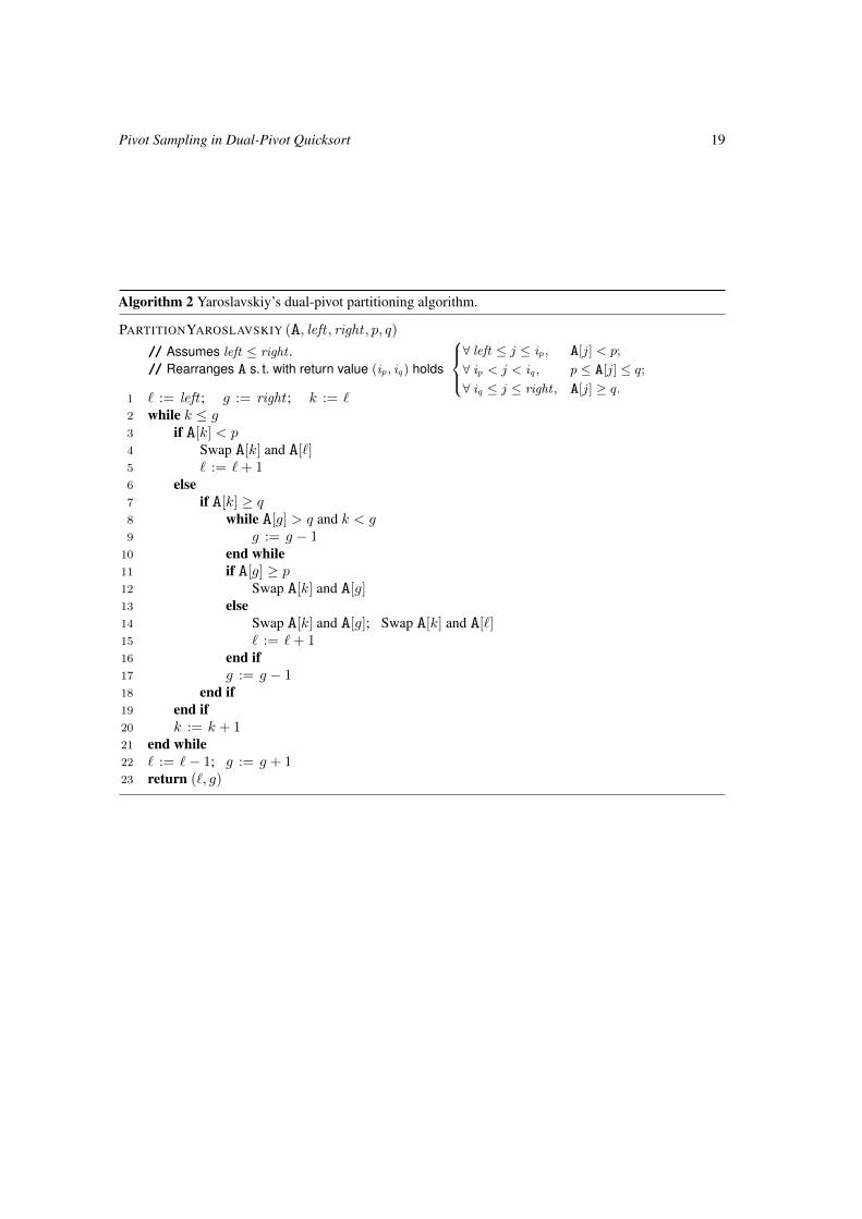
Algorithm 2 Yaroslavskiy’s dual-pivot partitioning algorithm.
PARTITIONYAROSLAVSKIY (A, left , right , p, q)
// Assumes left ≤ right .// Rearranges A s. t. with return value (ip , iq) holds
∀ left ≤ j ≤ ip , A[j] < p;
∀ ip < j < iq , p ≤ A[j] ≤ q;∀ iq ≤ j ≤ right , A[j] ≥ q.
1 ` := left ; g := right ; k := `2 while k ≤ g3 if A[k] < p4 Swap A[k] and A[`]5 ` := `+ 16 else7 if A[k] ≥ q8 while A[g] > q and k < g9 g := g − 1
10 end while11 if A[g] ≥ p12 Swap A[k] and A[g]13 else14 Swap A[k] and A[g]; Swap A[k] and A[`]15 ` := `+ 116 end if17 g := g − 118 end if19 end if20 k := k + 121 end while22 ` := `− 1; g := g + 123 return (`, g)
20 Markus E. Nebel and Sebastian Wild
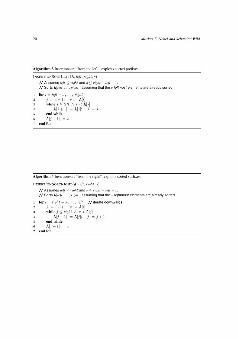
Algorithm 3 Insertionsort “from the left”, exploits sorted prefixes.
INSERTIONSORTLEFT(A, left , right , s)
// Assumes left ≤ right and s ≤ right − left − 1.// Sorts A[left , . . . , right ], assuming that the s leftmost elements are already sorted.
1 for i = left + s , . . . , right2 j := i− 1; v := A[i]3 while j ≥ left ∧ v < A[j]4 A[j + 1] := A[j]; j := j − 15 end while6 A[j + 1] := v7 end for
Algorithm 4 Insertionsort “from the right”, exploits sorted suffixes.
INSERTIONSORTRIGHT(A, left , right , s)
// Assumes left ≤ right and s ≤ right − left − 1.// Sorts A[left , . . . , right ], assuming that the s rightmost elements are already sorted.
1 for i = right − s , . . . , left // iterate downwards2 j := i+ 1; v := A[i]3 while j ≤ right ∧ v > A[j]4 A[j − 1] := A[j]; j := j + 15 end while6 A[j − 1] := v7 end for
Pivot Sampling in Dual-Pivot Quicksort 21
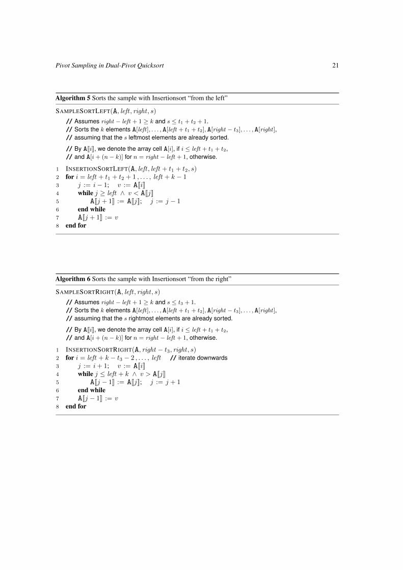
Algorithm 5 Sorts the sample with Insertionsort “from the left”
SAMPLESORTLEFT(A, left , right , s)
// Assumes right − left + 1 ≥ k and s ≤ t1 + t2 + 1.// Sorts the k elements A[left ], . . . ,A[left + t1 + t2],A[right − t3], . . . ,A[right ],// assuming that the s leftmost elements are already sorted.
// By AJiK, we denote the array cell A[i], if i ≤ left + t1 + t2,// and A[i+ (n− k)] for n = right − left + 1, otherwise.
1 INSERTIONSORTLEFT(A, left , left + t1 + t2, s)2 for i = left + t1 + t2 + 1 , . . . , left + k − 13 j := i− 1; v := AJiK4 while j ≥ left ∧ v < AJjK5 AJj + 1K := AJjK; j := j − 16 end while7 AJj + 1K := v8 end for
Algorithm 6 Sorts the sample with Insertionsort “from the right”
SAMPLESORTRIGHT(A, left , right , s)
// Assumes right − left + 1 ≥ k and s ≤ t3 + 1.// Sorts the k elements A[left ], . . . ,A[left + t1 + t2],A[right − t3], . . . ,A[right ],// assuming that the s rightmost elements are already sorted.
// By AJiK, we denote the array cell A[i], if i ≤ left + t1 + t2,// and A[i+ (n− k)] for n = right − left + 1, otherwise.
1 INSERTIONSORTRIGHT(A, right − t3, right , s)2 for i = left + k − t3 − 2 , . . . , left // iterate downwards3 j := i+ 1; v := AJiK4 while j ≤ left + k ∧ v > AJjK5 AJj − 1K := AJjK; j := j + 16 end while7 AJj − 1K := v8 end for
22 Markus E. Nebel and Sebastian Wild
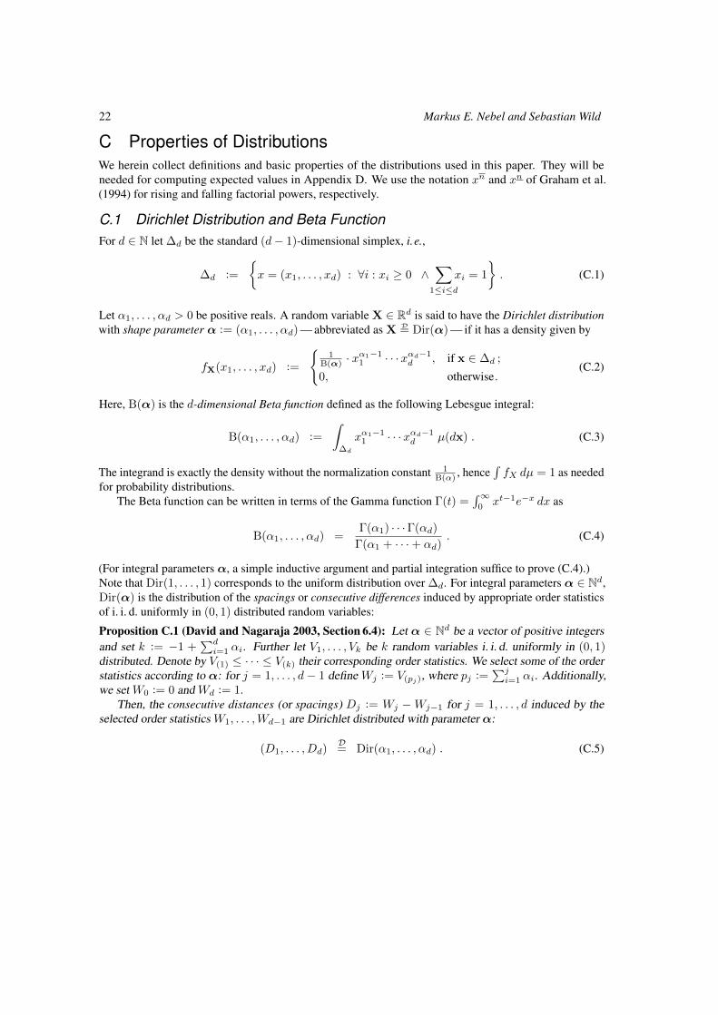
C Properties of DistributionsWe herein collect definitions and basic properties of the distributions used in this paper. They will beneeded for computing expected values in Appendix D. We use the notation xn and xn of Graham et al.(1994) for rising and falling factorial powers, respectively.
C.1 Dirichlet Distribution and Beta FunctionFor d ∈ N let ∆d be the standard (d− 1)-dimensional simplex, i.e.,
∆d :=
{x = (x1, . . . , xd) : ∀i : xi ≥ 0 ∧
∑1≤i≤d
xi = 1
}. (C.1)
Let α1, . . . , αd > 0 be positive reals. A random variable X ∈ Rd is said to have the Dirichlet distributionwith shape parameter α := (α1, . . . , αd) — abbreviated as X D= Dir(α) — if it has a density given by
fX(x1, . . . , xd) :=
{1
B(α) · xα1−11 · · ·xαd−1
d , if x ∈ ∆d ;
0, otherwise.(C.2)
Here, B(α) is the d-dimensional Beta function defined as the following Lebesgue integral:
B(α1, . . . , αd) :=
∫∆d
xα1−11 · · ·xαd−1
d µ(dx) . (C.3)
The integrand is exactly the density without the normalization constant 1B(α) , hence
∫fX dµ = 1 as needed
for probability distributions.The Beta function can be written in terms of the Gamma function Γ(t) =
∫∞0xt−1e−x dx as
B(α1, . . . , αd) =Γ(α1) · · ·Γ(αd)
Γ(α1 + · · ·+ αd). (C.4)
(For integral parameters α, a simple inductive argument and partial integration suffice to prove (C.4).)Note that Dir(1, . . . , 1) corresponds to the uniform distribution over ∆d. For integral parameters α ∈ Nd,Dir(α) is the distribution of the spacings or consecutive differences induced by appropriate order statisticsof i. i. d. uniformly in (0, 1) distributed random variables:
Proposition C.1 (David and Nagaraja 2003, Section 6.4): Let α ∈ Nd be a vector of positive integersand set k := −1 +
∑di=1 αi. Further let V1, . . . , Vk be k random variables i. i. d. uniformly in (0, 1)
distributed. Denote by V(1) ≤ · · · ≤ V(k) their corresponding order statistics. We select some of the orderstatistics according to α: for j = 1, . . . , d− 1 define Wj := V(pj), where pj :=
∑ji=1 αi. Additionally,
we set W0 := 0 and Wd := 1.Then, the consecutive distances (or spacings) Dj := Wj −Wj−1 for j = 1, . . . , d induced by the
selected order statistics W1, . . . ,Wd−1 are Dirichlet distributed with parameter α:
(D1, . . . , Dd)D= Dir(α1, . . . , αd) . (C.5)
Pivot Sampling in Dual-Pivot Quicksort 23
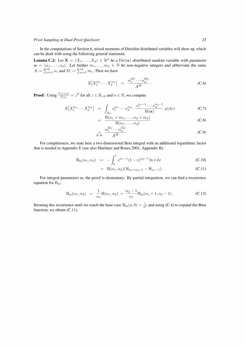
In the computations of Section 6, mixed moments of Dirichlet distributed variables will show up, whichcan be dealt with using the following general statement.
Lemma C.2: Let X = (X1, . . . , Xd) ∈ Rd be a Dir(α) distributed random variable with parameterα = (α1, . . . , αd). Let further m1, . . . ,md ∈ N be non-negative integers and abbreviate the sumsA :=
∑di=1 αi and M :=
∑di=1mi. Then we have
E[Xm1
1 · · ·Xmdd
]=
αm11 · · ·αmddAM
. (C.6)
Proof: Using Γ(z+n)Γ(z) = zn for all z ∈ R>0 and n ∈ N, we compute
E[Xm1
1 · · ·Xmdd
]=
∫∆d
xm11 · · ·xmdd ·
xα1−11 · · ·xαd−1
d
B(α)µ(dx) (C.7)
=B(α1 +m1, . . . , αd +md)
B(α1, . . . , αd)(C.8)
=(C.4)
αm11 · · ·αmddAM
. (C.9)
For completeness, we state here a two-dimensional Beta integral with an additional logarithmic factorthat is needed in Appendix E (see also Martínez and Roura 2001, Appendix B):
Bln(α1, α2) := −∫ 1
0
xα1−1(1− x)α2−1 lnx dx (C.10)
= B(α1, α2)(Hα1+α2−1 −Hα1−1) . (C.11)
For integral parameters α, the proof is elementary: By partial integration, we can find a recurrenceequation for Bln:
Bln(α1, α2) =1
α1B(α1, α2) +
α2 − 1
α1Bln(α1 + 1, α2 − 1) . (C.12)
Iterating this recurrence until we reach the base case Bln(a, 0) = 1a2 and using (C.4) to expand the Beta
function, we obtain (C.11).
24 Markus E. Nebel and Sebastian Wild
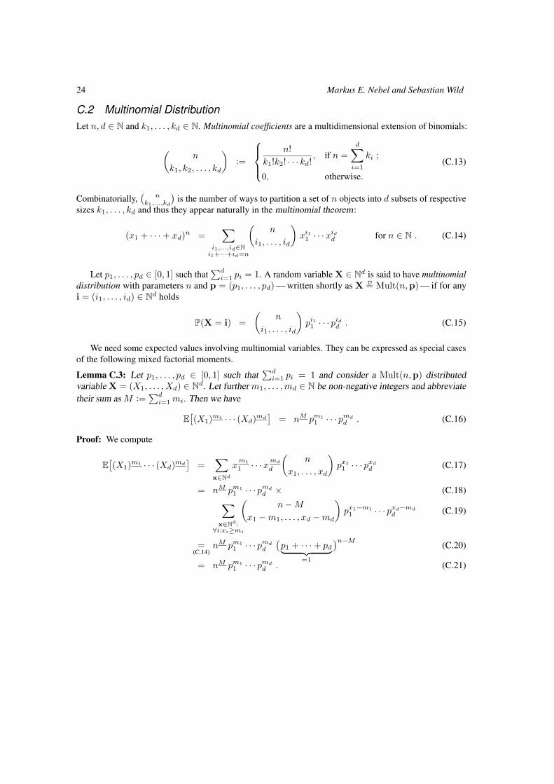
C.2 Multinomial DistributionLet n, d ∈ N and k1, . . . , kd ∈ N. Multinomial coefficients are a multidimensional extension of binomials:
(n
k1, k2, . . . , kd
):=
n!
k1!k2! · · · kd!, if n =
d∑i=1
ki ;
0, otherwise.
(C.13)
Combinatorially,(
nk1,...,kd
)is the number of ways to partition a set of n objects into d subsets of respective
sizes k1, . . . , kd and thus they appear naturally in the multinomial theorem:
(x1 + · · ·+ xd)n =
∑i1,...,id∈Ni1+···+id=n
(n
i1, . . . , id
)xi11 · · ·x
idd for n ∈ N . (C.14)
Let p1, . . . , pd ∈ [0, 1] such that∑di=1 pi = 1. A random variable X ∈ Nd is said to have multinomial
distribution with parameters n and p = (p1, . . . , pd) — written shortly as X D= Mult(n,p) — if for anyi = (i1, . . . , id) ∈ Nd holds
P(X = i) =
(n
i1, . . . , id
)pi11 · · · p
idd . (C.15)
We need some expected values involving multinomial variables. They can be expressed as special casesof the following mixed factorial moments.
Lemma C.3: Let p1, . . . , pd ∈ [0, 1] such that∑di=1 pi = 1 and consider a Mult(n,p) distributed
variable X = (X1, . . . , Xd) ∈ Nd. Let further m1, . . . ,md ∈ N be non-negative integers and abbreviatetheir sum as M :=
∑di=1mi. Then we have
E[(X1)m1 · · · (Xd)
md]
= nM pm11 · · · pmdd . (C.16)
Proof: We compute
E[(X1)m1 · · · (Xd)
md]
=∑x∈Nd
xm1
1 · · ·xmdd
(n
x1, . . . , xd
)px1
1 · · · pxdd (C.17)
= nM pm11 · · · pmdd × (C.18)∑
x∈Nd:∀i:xi≥mi
(n−M
x1 −m1, . . . , xd −md
)px1−m1
1 · · · pxd−mdd (C.19)
=(C.14)
nM pm11 · · · pmdd
(p1 + · · ·+ pd︸ ︷︷ ︸
=1
)n−M(C.20)
= nM pm11 · · · pmdd . (C.21)
Pivot Sampling in Dual-Pivot Quicksort 25
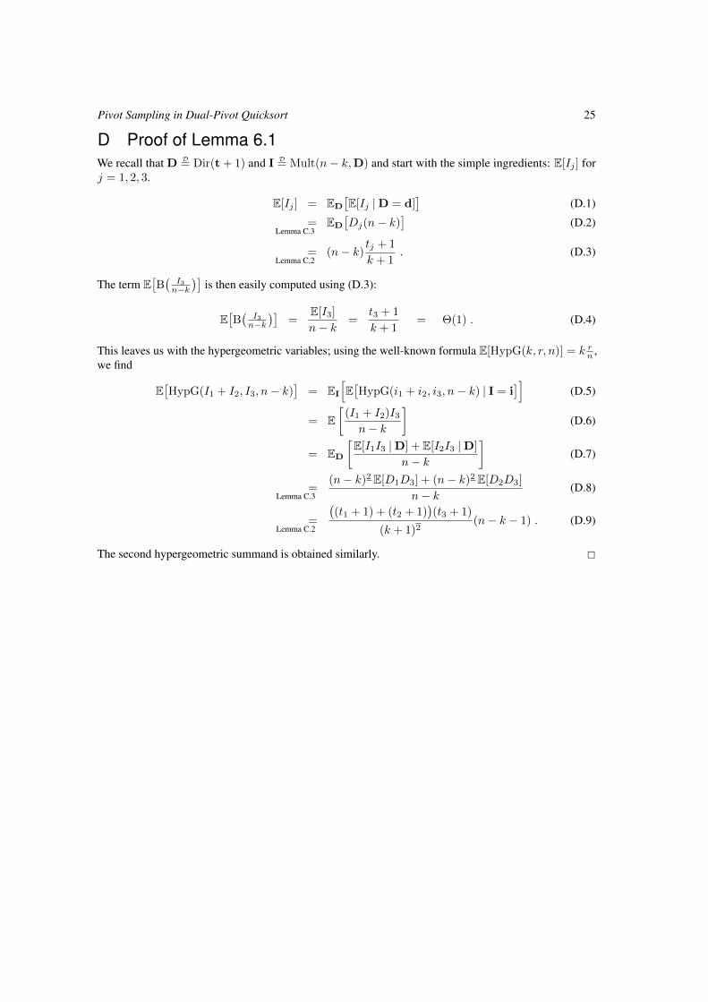
D Proof of Lemma 6.1We recall that D D= Dir(t + 1) and I D= Mult(n− k,D) and start with the simple ingredients: E[Ij ] forj = 1, 2, 3.
E[Ij ] = ED
[E[Ij |D = d]
](D.1)
=Lemma C.3
ED
[Dj(n− k)
](D.2)
=Lemma C.2
(n− k)tj + 1
k + 1. (D.3)
The term E[B(I3n−k
)]is then easily computed using (D.3):
E[B(I3n−k
)]=
E[I3]
n− k=
t3 + 1
k + 1= Θ(1) . (D.4)
This leaves us with the hypergeometric variables; using the well-known formula E[HypG(k, r, n)] = k rn ,we find
E[HypG(I1 + I2, I3, n− k)
]= EI
[E[HypG(i1 + i2, i3, n− k) | I = i
]](D.5)
= E[
(I1 + I2)I3n− k
](D.6)
= ED
[E[I1I3 |D] + E[I2I3 |D]
n− k
](D.7)
=Lemma C.3
(n− k)2 E[D1D3] + (n− k)2 E[D2D3]
n− k(D.8)
=Lemma C.2
((t1 + 1) + (t2 + 1)
)(t3 + 1)
(k + 1)2(n− k − 1) . (D.9)
The second hypergeometric summand is obtained similarly. 2
26 Markus E. Nebel and Sebastian Wild
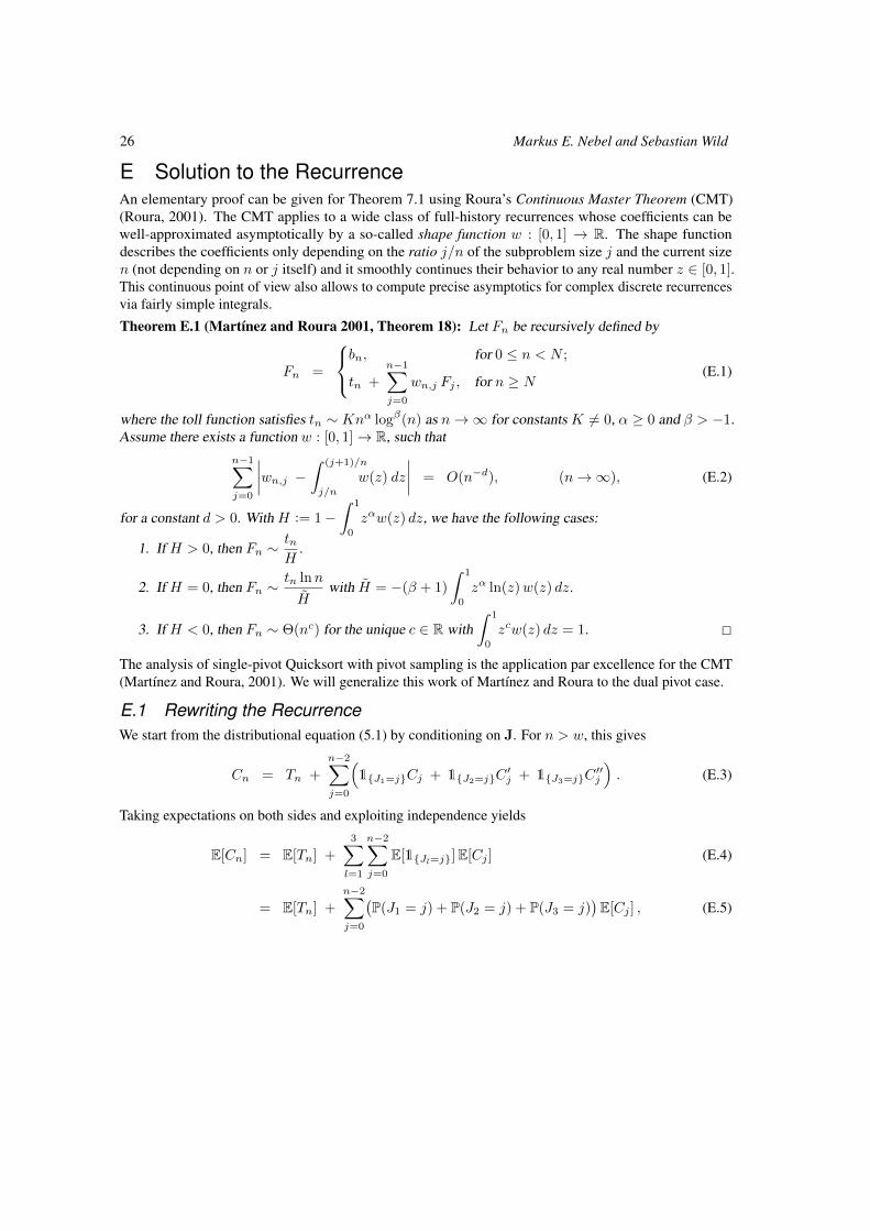
E Solution to the RecurrenceAn elementary proof can be given for Theorem 7.1 using Roura’s Continuous Master Theorem (CMT)(Roura, 2001). The CMT applies to a wide class of full-history recurrences whose coefficients can bewell-approximated asymptotically by a so-called shape function w : [0, 1] → R. The shape functiondescribes the coefficients only depending on the ratio j/n of the subproblem size j and the current sizen (not depending on n or j itself) and it smoothly continues their behavior to any real number z ∈ [0, 1].This continuous point of view also allows to compute precise asymptotics for complex discrete recurrencesvia fairly simple integrals.
Theorem E.1 (Martínez and Roura 2001, Theorem 18): Let Fn be recursively defined by
Fn =
bn, for 0 ≤ n < N ;
tn +
n−1∑j=0
wn,j Fj , for n ≥ N(E.1)
where the toll function satisfies tn ∼ Knα logβ(n) as n→∞ for constants K 6= 0, α ≥ 0 and β > −1.Assume there exists a function w : [0, 1]→ R, such that
n−1∑j=0
∣∣∣∣wn,j − ∫ (j+1)/n
j/n
w(z) dz
∣∣∣∣ = O(n−d), (n→∞), (E.2)
for a constant d > 0. With H := 1−∫ 1
0
zαw(z) dz, we have the following cases:
1. If H > 0, then Fn ∼tnH
.
2. If H = 0, then Fn ∼tn lnn
H̃with H̃ = −(β + 1)
∫ 1
0
zα ln(z)w(z) dz.
3. If H < 0, then Fn ∼ Θ(nc) for the unique c ∈ R with∫ 1
0
zcw(z) dz = 1. 2
The analysis of single-pivot Quicksort with pivot sampling is the application par excellence for the CMT(Martínez and Roura, 2001). We will generalize this work of Martínez and Roura to the dual pivot case.
E.1 Rewriting the RecurrenceWe start from the distributional equation (5.1) by conditioning on J. For n > w, this gives
Cn = Tn +
n−2∑j=0
(1{J1=j}Cj + 1{J2=j}C
′j + 1{J3=j}C
′′j
). (E.3)
Taking expectations on both sides and exploiting independence yields
E[Cn] = E[Tn] +
3∑l=1
n−2∑j=0
E[1{Jl=j}]E[Cj ] (E.4)
= E[Tn] +
n−2∑j=0
(P(J1 = j) + P(J2 = j) + P(J3 = j)
)E[Cj ] , (E.5)
Pivot Sampling in Dual-Pivot Quicksort 27
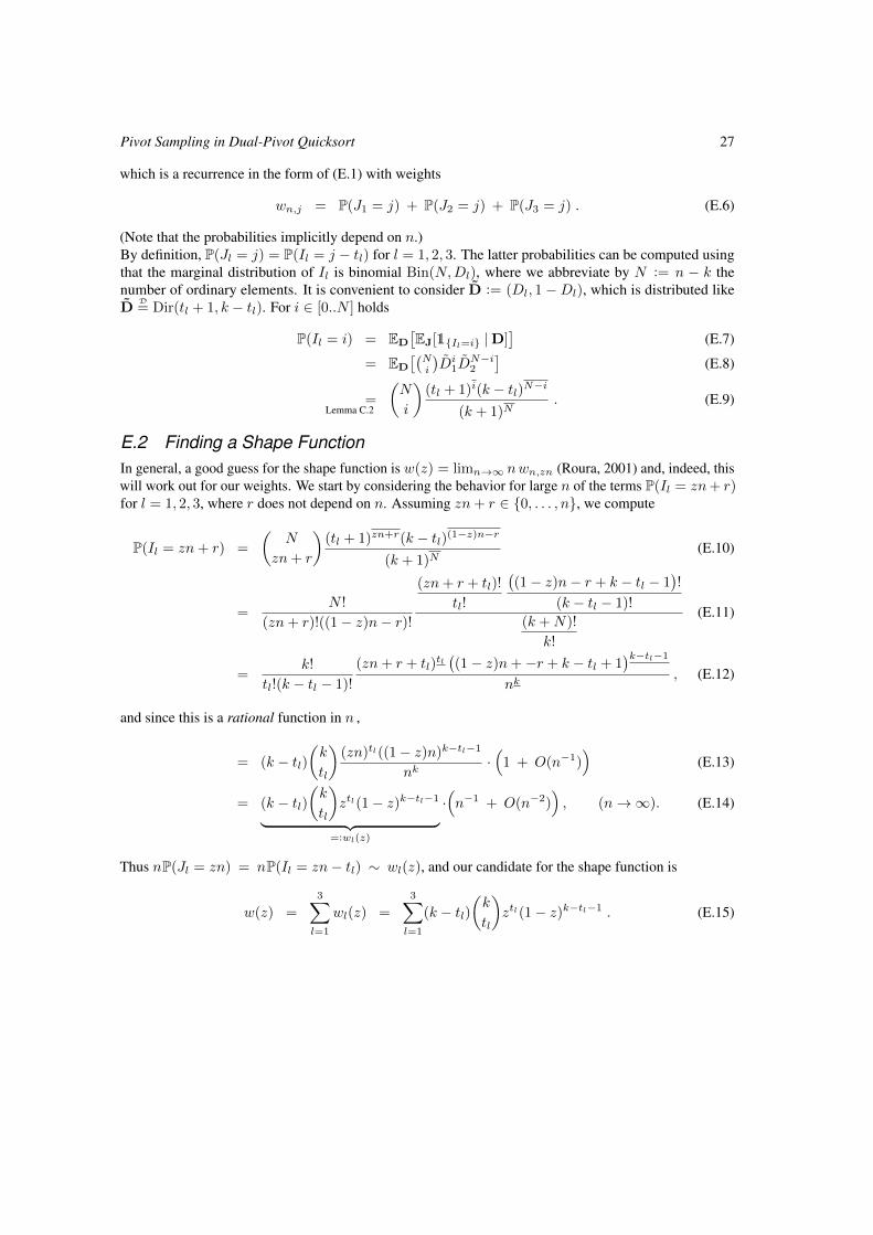
which is a recurrence in the form of (E.1) with weights
wn,j = P(J1 = j) + P(J2 = j) + P(J3 = j) . (E.6)
(Note that the probabilities implicitly depend on n.)By definition, P(Jl = j) = P(Il = j − tl) for l = 1, 2, 3. The latter probabilities can be computed usingthat the marginal distribution of Il is binomial Bin(N,Dl), where we abbreviate by N := n − k thenumber of ordinary elements. It is convenient to consider D̃ := (Dl, 1 −Dl), which is distributed likeD̃
D= Dir(tl + 1, k − tl). For i ∈ [0..N ] holds
P(Il = i) = ED
[EJ[1{Il=i} |D]
](E.7)
= ED
[(Ni
)D̃i
1D̃N−i2
](E.8)
=Lemma C.2
(N
i
)(tl + 1)i(k − tl)N−i
(k + 1)N. (E.9)
E.2 Finding a Shape FunctionIn general, a good guess for the shape function is w(z) = limn→∞ nwn,zn (Roura, 2001) and, indeed, thiswill work out for our weights. We start by considering the behavior for large n of the terms P(Il = zn+ r)for l = 1, 2, 3, where r does not depend on n. Assuming zn+ r ∈ {0, . . . , n}, we compute
P(Il = zn+ r) =
(N
zn+ r
)(tl + 1)zn+r(k − tl)(1−z)n−r
(k + 1)N(E.10)
=N !
(zn+ r)!((1− z)n− r)!
(zn+ r + tl)!
tl!
((1− z)n− r + k − tl − 1
)!
(k − tl − 1)!
(k +N)!
k!
(E.11)
=k!
tl!(k − tl − 1)!
(zn+ r + tl)tl((1− z)n+−r + k − tl + 1
)k−tl−1
nk, (E.12)
and since this is a rational function in n ,
= (k − tl)(k
tl
)(zn)tl((1− z)n)k−tl−1
nk·(
1 + O(n−1))
(E.13)
= (k − tl)(k
tl
)ztl(1− z)k−tl−1︸ ︷︷ ︸
=:wl(z)
·(n−1 + O(n−2)
), (n→∞). (E.14)
Thus nP(Jl = zn) = nP(Il = zn− tl) ∼ wl(z), and our candidate for the shape function is
w(z) =
3∑l=1
wl(z) =
3∑l=1
(k − tl)(k
tl
)ztl(1− z)k−tl−1 . (E.15)
28 Markus E. Nebel and Sebastian Wild
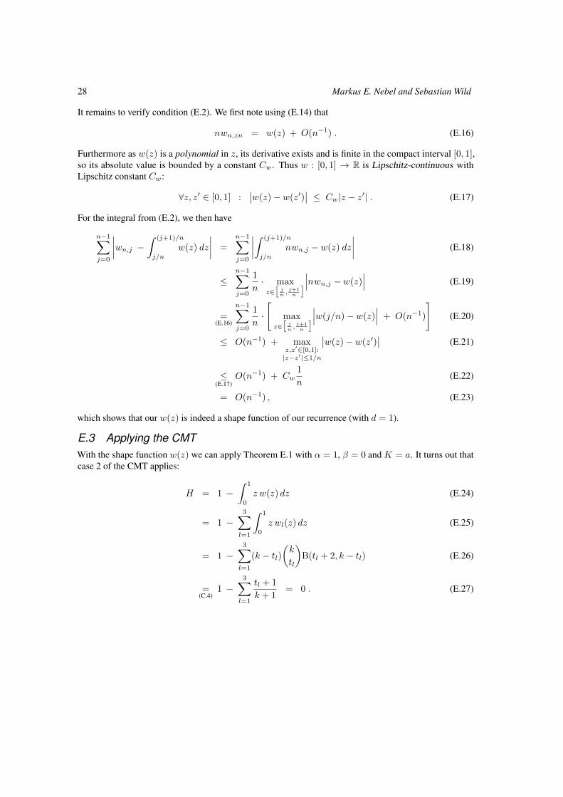
It remains to verify condition (E.2). We first note using (E.14) that
nwn,zn = w(z) + O(n−1) . (E.16)
Furthermore as w(z) is a polynomial in z, its derivative exists and is finite in the compact interval [0, 1],so its absolute value is bounded by a constant Cw. Thus w : [0, 1] → R is Lipschitz-continuous withLipschitz constant Cw:
∀z, z′ ∈ [0, 1] :∣∣w(z)− w(z′)
∣∣ ≤ Cw|z − z′| . (E.17)
For the integral from (E.2), we then have
n−1∑j=0
∣∣∣∣wn,j − ∫ (j+1)/n
j/n
w(z) dz
∣∣∣∣ =
n−1∑j=0
∣∣∣∣∫ (j+1)/n
j/n
nwn,j − w(z) dz
∣∣∣∣ (E.18)
≤n−1∑j=0
1
n· maxz∈[jn ,j+1n
]∣∣∣nwn,j − w(z)∣∣∣ (E.19)
=(E.16)
n−1∑j=0
1
n·
[max
z∈[jn ,j+1n
]∣∣∣w(j/n)− w(z)∣∣∣ + O(n−1)
](E.20)
≤ O(n−1) + maxz,z′∈[0,1]:|z−z′|≤1/n
∣∣w(z)− w(z′)∣∣ (E.21)
≤(E.17)
O(n−1) + Cw1
n(E.22)
= O(n−1) , (E.23)
which shows that our w(z) is indeed a shape function of our recurrence (with d = 1).
E.3 Applying the CMTWith the shape function w(z) we can apply Theorem E.1 with α = 1, β = 0 and K = a. It turns out thatcase 2 of the CMT applies:
H = 1 −∫ 1
0
z w(z) dz (E.24)
= 1 −3∑l=1
∫ 1
0
z wl(z) dz (E.25)
= 1 −3∑l=1
(k − tl)(k
tl
)B(tl + 2, k − tl) (E.26)
=(C.4)
1 −3∑l=1
tl + 1
k + 1= 0 . (E.27)
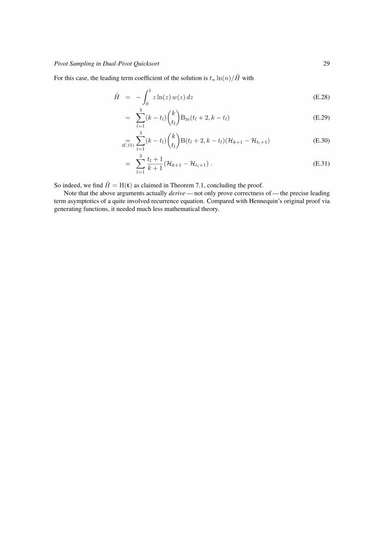
Pivot Sampling in Dual-Pivot Quicksort 29
For this case, the leading term coefficient of the solution is tn ln(n)/H̃ with
H̃ = −∫ 1
0
z ln(z)w(z) dz (E.28)
=
3∑l=1
(k − tl)(k
tl
)Bln(tl + 2, k − tl) (E.29)
=(C.11)
3∑l=1
(k − tl)(k
tl
)B(tl + 2, k − tl)(Hk+1 −Htl+1) (E.30)
=
3∑l=1
tl + 1
k + 1(Hk+1 −Htl+1) . (E.31)
So indeed, we find H̃ = H(t) as claimed in Theorem 7.1, concluding the proof.Note that the above arguments actually derive — not only prove correctness of — the precise leading
term asymptotics of a quite involved recurrence equation. Compared with Hennequin’s original proof viagenerating functions, it needed much less mathematical theory.


![Pivot Sampling in Dual-Pivot Quicksort - Aofa 2014 · 2014. 6. 21. · Pivot Sampling in Dual-Pivot Quicksort Sebastian Wild Markus E. Nebel [wild,nebel]@cs.uni-kl.de 16 June 2014](https://img.pdfslide.us/doc/110x75/604cdd46fed1b4604c61f9a4/pivot-sampling-in-dual-pivot-quicksort-aofa-2014-6-21-pivot-sampling-in-dual-pivot.jpg)