Pitfalls in the Use of Time Series Methods to Study

ORI GIN AL PA PER

Pitfalls in the Use of Time Series Methods to StudyDeterrence and Capital Punishment

Kerwin Kofi Charles • Steven N. Durlauf

Published online: 24 February 2012� Springer Science+Business Media, LLC 2012

AbstractObjectives Evaluate the use of various time series methods to measure the deterrence

effect of capital punishment.

Methods The analysis of the time series approach to deterrence is conducted at two

levels. First, the mathematical foundations of time series methods are described and the

link between the time series properties of aggregate homicide and execution series and

individual decision making is developed. Second, individual studies are examined for

logical consistency.

Results The analysis concludes that time series methods used to study the deterrence

effects of capital punishment suffer from fundamental limitations and fail to provide

credible evidence. The common limitation of these studies is their lack of attention to

identification problems. Suggestions are made as to directions for future work that may be

able to mitigate the weaknesses of the current literature.

Conclusions Time series studies of capital punishment suffer from sufficiently serious

identification problems that existing empirical findings are compatible with either the

presence or the absence of a deterrent effect.

Keywords Capital punishment � Deterrence � Brutalization � Identification �Decision theory

K. K. CharlesUniversity of Chicago, Chicago, IL, USA

S. N. Durlauf (&)Department of Economics, University of Wisconsin,1180 Observatory Drive, Madison, WI 53706, USAe-mail: [email protected]

123

J Quant Criminol (2013) 29:45–66DOI 10.1007/s10940-012-9169-7

Introduction

In this paper we evaluate the use of time series methods to uncover a deterrent effect to

capital punishment.1 While much of the recent deterrence literature has focused on panel

data sets, there is a continuing literature that is based on the analysis of time series to infer

deterrent effects. While the studies we examine can be thought of as panels with a cross

sectional dimension of one or two, it is appropriate to distinguish them from panel data

studies both because the studies are all driven by temporal variation and because the

methods that underlie their approach to deterrence are very different from those found in

the current panel literature. In particular, the time series approaches we study are much less

closely tied to behavioral models of potential murderers than are the panel studies.

As will be clear, we do not believe that these approaches have provided any causal

evidence on the deterrence question. This is admittedly a very strong claim, but one that we

believe can be sustained. While our discussion will focus on a set of particular papers, we

believe that this set is representative of the overall time series literature on capital pun-

ishment and deterrence, and so we regard our critique of these individual analyses as a

general commentary on one class of deterrence exercises for capital punishment. Further,

our criticisms are not unique to capital punishment; they also apply with equal force to the

use of these methods to study the deterrent effects of imprisonment, for example.

Some of the methods used to study capital punishment originated in the application of

rigorous time series methodology to macroeconomics.2 Since their introduction, economists

have had spirited disagreements about how these methods might be used to address positive

questions, and especially issues related to policy evaluation. In our discussion of these time series

methods as applied to the study of deterrence, we emphasize arguments for which we believe is

overwhelming and possibly universal acceptance among theoretical and applied time series

econometricians who have formally studied the strengths and limitations of these methods.

The term ‘‘time series methods’’ encompasses a broad spectrum of methods. We therefore

consider three distinct ways in which time series approaches have been used to study capital

punishment and deterrence. Section ‘‘Atheoretical Time Series Models and Causality

Approaches to Deterrence’’ focuses on the use of causality tests to evaluate deterrence.

Section ‘‘Event Studies’’ examines event studies involving specific executions. Section

‘‘Regression Studies’’ considers some general time series regressions. Section ‘‘Cross Polity

Comparisons’’ examines the use of comparisons of time series between political units, one

with and the other without capital punishment. Section ‘‘Conceptual Issues’’ suggests some

general messages about the weaknesses in the use of time series methods to study capital

punishment and deterrence that are suggested by our detailed critiques of papers in the

existing literature, and Section ‘‘Conclusions: Why Time Series?’’ concludes.

Atheoretical Time Series Models and Causality Approaches to Deterrence

Conceptual Background

One methodology used in time series studies of deterrence is known as vector autore-

gressions (VARs). Research of this type estimates dynamic regressions relating current

1 We refer to ‘‘a’’ rather than ‘‘the’’ deterrent effect as different papers employ different deterrence mea-sures which have different substantive interpretations.2 In this regard, Granger (1969) and Sims (1972, 1980, 1982) play foundational roles.

46 J Quant Criminol (2013) 29:45–66

123

homicide and execution rates to previous realizations of these two variables. The estimated

relationships are then used to make inference about deterrence. While this methodology has

only recently been applied in capital punishment and deterrence studies, it has been long used

in studies of imprisonment and crime; see Durlauf and Nagin (2010) for a review. We

extensively review the potential shortcomings of this method as a source of information on

deterrence effects because it is currently the methodological state of the art in time series

deterrence studies and so we are concerned that in the future it will be more widely used.

A distinct feature of this approach is that it is essentially atheoretical—in the sense that

the approach does not first posit a behavioral model relating the decision to commit a

homicide to the distribution of outcomes if the act is committed, including the possibility

of execution and then aggregates up individual choices to determine how a deterrence

effect would restrict the joint stochastic processes for murders and executions. This feature

of this branch of the time series literature on deterrence and capital punishment is similar to

the ‘‘atheoretical’’ tradition in empirical macroeconomics.3 In drawing a dichotomy

between atheoretical and theoretical approaches to empirical analysis, we are really dis-

tinguishing between statistical models of social science data which may be subject to ex

post interpretation using social science theory versus statistical models that are derived

from a social science theory. It is of course possible to construct statistical models whose

structure is partly restricted by social science theory. One sees this in the so-called

structural vector autoregression literature in which economic theory is used to restrict the

variance covariance matrix of model errors while the dynamics present in the data are

unrestricted. Nevertheless, the distinction between the two approaches provides a basis for

understanding alternative empirical strategies.

In this section, we provide a description of the basic time series properties that have

been used to draw atheoretical conclusions about the deterrent effects of the death penalty.

We argue that these properties do not justify the substantive interpretations that they have

received, and then provide two examples of papers where this problem arises. Our dis-

cussion of time series is intentionally heuristic. Ash and Gardner (1975) provides a fully

rigorous treatment that we recommend for clarity, although the formalization of our pre-

sentation may be found in many advanced texts on stochastic processes (Hamilton (1994)

has become the standard reference for economists). While we focus on the death penalty,

our arguments naturally generalize to analogous time series models of deterrence and

imprisonment, such as Marvell and Moody (1994), Becsi (1999), and Spelman (2000).

For notational purposes, we denote the number of homicides in political unit i at time t as

Hit; Eit denotes the number of executions in unit i at t. The focus on political units reflects the

use of aggregate data in the time series/deterrence literature. The rates (with respect to the

population of i at t) of these variables are in turn denoted as hit and eit. The choice between

levels and rates varies across studies. For expositional purposes, we focus on the joint

properties of the homicide and execution levels, but all of our discussion applies to their

associated rates. It should be noted that the validity of the assumptions under which time

series analyses of capital punishment and deterrence are conducted may depend on whether

the analysis is based on rates or levels, but we do not pursue this issue here.

3 Early time series studies of capital punishment and deterrence, notably Ehrlich (1975a, b) were notatheoretical in the sense in which we use the term and in fact followed a version what we have called astructural strategy. While Ehrlich’s work was subjected to serious criticism to the extent that a NationalAcademy of Sciences panel concluded his empirical claims were too fragile to warrant acceptance(Blumstein et al. 1978), Ehrlich’s pioneering strategy of using economic theory to motivate the statisticalmodels under study should be recognized. Ehrlich’s approach is followed in the modern panel data approachto capital punishment and deterrence, e.g. Dezhbakhsh et al. (2003).

J Quant Criminol (2013) 29:45–66 47

123

In times series studies of deterrence, homicide and execution levels are usually con-

ceptualized as being decomposed into deterministic and stochastic components. Thus, they

are assumed to be given by

Hi;t ¼ HDi;t þ HS

i;t ð1Þ

and

Ei;t ¼ EDi;t þ ES

i;t: ð2Þ

In the empirical literature, the deterministic terms HDi;t and ED

i;t are commonly modeled as

consisting of a constant term and some function of time—a formulation that is obviously

somewhat ad hoc. A different way to think about the deterministic/stochastic distinction is

based on the Wold decomposition theorem. By that theorem, under the assumptions that

(1) each series has an unconditional zero mean, that (2) each series has a finite variance,

and that (3) each series is second order stationary,4 the deterministic component of a time

series possesses a particular interpretation: it is the part of the time series that can be

predicted from the arbitrary past, where predictions are restricted to linear combinations of

the lagged levels of the series or limits of such linear combinations. One interpretation of

detrending methods of the type commonly used in the empirical literature on deterrence is

that detrending is needed to justify the assumptions underlying the Wold decomposition

theorem, although this interpretation is not typically explicitly invoked.

Regardless of how one conceptualizes the deterministic components, the primary focus

in time series deterrence studies is on the stochastic terms in these series; we will therefore

restrict our attention to these terms. In particular, under the assumptions of the Wold

theorem (which we assume hold for the stochastic components of the time series, with the

Wold notion of a deterministic component included in HDi;t and ED

i;t, respectively), these

components can be decomposed as

HSi;t

ESi;t

� �¼ p11 Lð Þ p12 Lð Þ

p21 Lð Þ p22 Lð Þ

� �ei;t

gi;t

� �ð3Þ

where the terms pij Lð Þ are one side lag polynomials.5 The shocks (also called innovations)

ei;t and gi;t have an important interpretation: each represents the one step-ahead prediction

error of the respective time series on the left hand side of Eq. 3 for the best prediction of

the time series given the joint histories of the times series, when (1) ‘‘best’’ means having

minimum prediction error variance among all predictions and (2) predictions are required

to be linear combinations of the levels of the time series or the limits of such linear

combinations.6 When the lag operator matrixp11 Lð Þ p12 Lð Þp21 Lð Þ p22 Lð Þ

� �matrix is invertible,

which means that each series has an autoregressive representation—that is, one can rewrite

the series as

4 Second order stationarity means that cov HSi;t;H

Si;t�j

� �, cov ES

i;t;ESi;t�j

� �, and cov HS

i;t;ESi;t�j

� �does not

depend on t, for all �1\j\1: Intuitively, second order stationarity imposes an invariance on the timeseries under study that produces time invariant moving average and autoregressive coefficients.5 The lag operator Lk maps xt to xt�k , i.e. Lkxt ¼ xt�k . A lag polynomial is one sided if none of the terms

Lkpossesses a negative exponent.6 The shocks in this representation are sometimes called the fundamental innovations for the processesunder study, to indicate that they represent one step ahead prediction errors.


123

HSi;t

ESi;t

� �¼ b11 Lð Þ b12 Lð Þ

b21 Lð Þ b22 Lð Þ

� �HS

i;t�1

ESi;t�1

� �þ ei;t

gi;t

� �ð4Þ

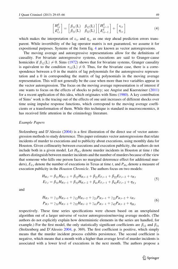
which makes the interpretation of ei;t and gi;t as one step ahead prediction errors trans-

parent. While invertibility of the lag operator matrix is not guaranteed, we assume it for

expositional purposes. Systems of the form Eq. 4 are known as vector autoregressions.

The moving average and autoregressive representations allow for the definitions of

causality. For bivariate autoregressive systems, executions are said to Granger-cause

homicides if b12 Lð Þ 6¼ 0. Sims (1972) shows that for bivariate systems, Granger causality

is equivalent to the condition p12 Lð Þ 6¼ 0. Thus, for the bivariate case, there is a corre-

spondence between a 0 in the matrix of lag polynomials for the autoregressive represen-

tation and a 0 in corresponding the matrix of lag polynomials in the moving average

representation. This will not generally be the case when more than two variables appear in

the vector autoregression. The focus on the moving average representation is of interest if

one wants to focus on the effects of shocks to policy; see Angrist and Kuersteiner (2011)

for a recent application of this idea, which originates with Sims (1980). A key contribution

of Sims’ work is the tracing out of the effects of one unit increases of different shocks over

time using impulse response functions, which correspond to the moving average coeffi-

cients or a transformation of them. While this technique is standard in macroeconomics, it

has received little attention in the criminology literature.

Example Papers

Stolzenberg and D’Alessio (2004) is a first illustration of the direct use of vector autore-

gression methods to study deterrence. This paper estimates vector autoregressions that relate

incidents of murder to executions and to publicity about executions, using monthly data for

Houston. Given collinearity between executions and execution publicity, the authors do not

include both in a given model. Let HH,t denote murder incidents in Houston at time t (the

authors distinguish between murder incidents and the number of murders because of the view

that someone who kills one person faces no marginal deterrence effect for additional mur-

ders), ET,t denote the number of executions in Texas at time t, and PH,t denote a measure of

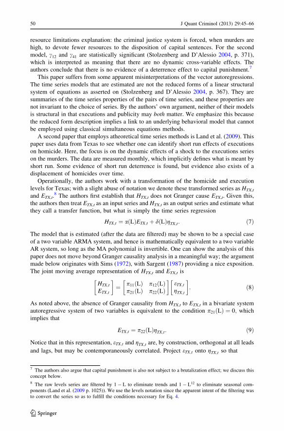
execution publicity in the Houston Chronicle. The authors focus on two models:

HH;t ¼ b11HH;t�1 þ b12HH;t�2 þ b21ET ;t�1 þ b22ET ;t�2 þ eH;t

ET ;t ¼ b31HH;t�1 þ b32HH;t�2 þ b41ET ;t�1 þ b42ET ;t�2 þ gT ;t

ð5Þ

and

HH;t ¼ c11HH;t�1 þ c12HH;t�2 þ c21PH;t�1 þ c22PH;t�2 þ eH;t

PH;t ¼ c31HH;t�1 þ c32HH;t�2 þ c41PH;t�1 þ c42PH;t�2 þ gH;t

ð6Þ

respectively. These time series specifications were chosen based on an unexplained

algorithm out of a larger universe of vector autoregression/moving average models. (The

authors do not explicitly explain how deterministic elements in the series are handled, for

example.) For the first model, the only statistically significant coefficients are b12 and b31

(Stolzenberg and D’Alessio 2004, p. 369). The first coefficient is positive, which simply

means that the murder incident process exhibits persistence. The second coefficient is

negative, which means that a month with a higher than average level of murder incidents is

associated with a lower level of executions in the next month. The authors propose a


123

resource limitations explanation: the criminal justice system is forced, when murders are

high, to devote fewer resources to the disposition of capital sentences. For the second

model, c12 and c41 are statistically significant (Stolzenberg and D’Alessio 2004, p. 371),

which is interpreted as meaning that there are no dynamic cross-variable effects. The

authors conclude that there is no evidence of a deterrence effect to capital punishment.7

This paper suffers from some apparent misinterpretations of the vector autoregressions.

The time series models that are estimated are not the reduced forms of a linear structural

system of equations as asserted on (Stolzenberg and D’Alessio 2004, p. 367). They are

summaries of the time series properties of the pairs of time series, and these properties are

not invariant to the choice of series. By the authors’ own argument, neither of their models

is structural in that executions and publicity may both matter. We emphasize this because

the reduced form description implies a link to an underlying behavioral model that cannot

be employed using classical simultaneous equations methods.

A second paper that employs atheoretical time series methods is Land et al. (2009). This

paper uses data from Texas to see whether one can identify short run effects of executions

on homicide. Here, the focus is on the dynamic effects of a shock to the executions series

on the murders. The data are measured monthly, which implicitly defines what is meant by

short run. Some evidence of short run deterrence is found, but evidence also exists of a

displacement of homicides over time.

Operationally, the authors work with a transformation of the homicide and execution

levels for Texas; with a slight abuse of notation we denote these transformed series as HTX,t

and ETX,t.8 The authors first establish that HTX,t does not Granger cause ETX,t. Given this,

the authors then treat ETX,t as an input series and HTX,t as an output series and estimate what

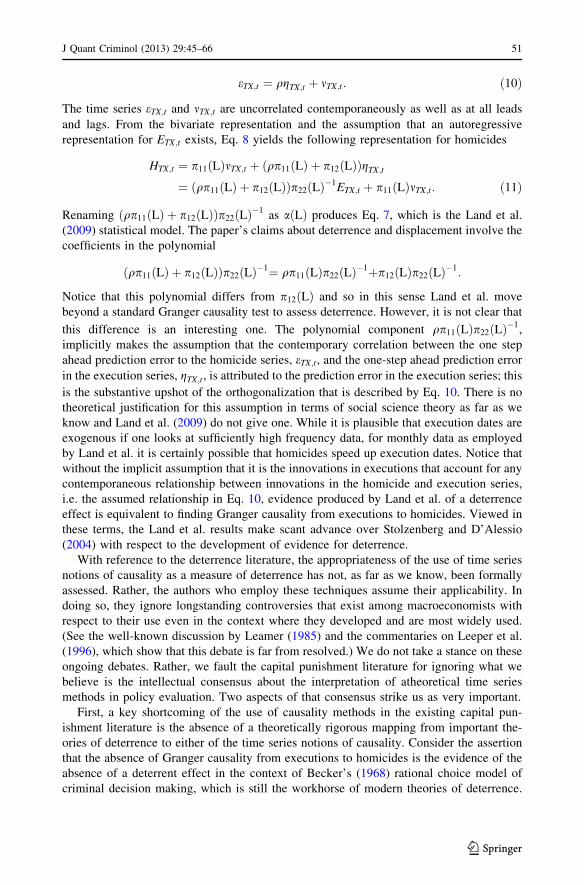
they call a transfer function, but what is simply the time series regression

HTX;t ¼ a Lð ÞETX;t þ d Lð ÞgTX;t: ð7Þ

The model that is estimated (after the data are filtered) may be shown to be a special case

of a two variable ARMA system, and hence is mathematically equivalent to a two variable

AR system, so long as the MA polynomial is invertible. One can show the analysis of this

paper does not move beyond Granger causality analysis in a meaningful way; the argument

made below originates with Sims (1972), with Sargent (1987) providing a nice exposition.

The joint moving average representation of HTX,t and ETX,t is

HTX;t

ETX;t

� �¼ p11 Lð Þ p12 Lð Þ

p21 Lð Þ p22 Lð Þ

� �eTX;t

gTX;t

� �: ð8Þ

As noted above, the absence of Granger causality from HTX,t to ETX,t in a bivariate system

autoregressive system of two variables is equivalent to the condition p21 Lð Þ ¼ 0; which

implies that

ETX;t ¼ p22 Lð ÞgTX;t: ð9Þ

Notice that in this representation, eTX;t and gTX;t are, by construction, orthogonal at all leads

and lags, but may be contemporaneously correlated. Project eTX;t onto gTX;t so that

7 The authors also argue that capital punishment is also not subject to a brutalization effect; we discuss thisconcept below.8 The raw levels series are filtered by 1� L to eliminate trends and 1� L12 to eliminate seasonal com-ponents (Land et al. (2009 p. 1025)). We use the levels notation since the apparent intent of the filtering wasto convert the series so as to fulfill the conditions necessary for Eq. 4.


123

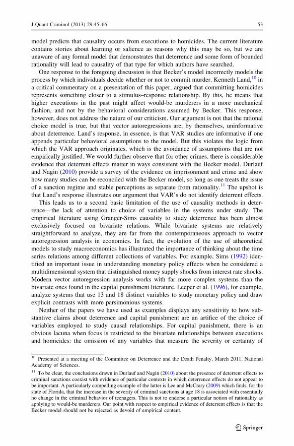
eTX;t ¼ qgTX;t þ mTX;t: ð10Þ

The time series eTX;t and mTX;t are uncorrelated contemporaneously as well as at all leads

and lags. From the bivariate representation and the assumption that an autoregressive

representation for ETX;t exists, Eq. 8 yields the following representation for homicides

HTX;t ¼ p11 Lð ÞmTX;t þ qp11 Lð Þ þ p12 Lð Þð ÞgTX;t

¼ qp11 Lð Þ þ p12 Lð Þð Þp22 Lð Þ�1ETX;t þ p11 Lð ÞmTX;t: ð11Þ

Renaming qp11 Lð Þ þ p12 Lð Þð Þp22 Lð Þ�1as a Lð Þ produces Eq. 7, which is the Land et al.

(2009) statistical model. The paper’s claims about deterrence and displacement involve the

coefficients in the polynomial

qp11 Lð Þ þ p12 Lð Þð Þp22 Lð Þ�1¼ qp11 Lð Þp22 Lð Þ�1þp12 Lð Þp22 Lð Þ�1:

Notice that this polynomial differs from p12 Lð Þ and so in this sense Land et al. move

beyond a standard Granger causality test to assess deterrence. However, it is not clear that

this difference is an interesting one. The polynomial component qp11 Lð Þp22 Lð Þ�1,

implicitly makes the assumption that the contemporary correlation between the one step

ahead prediction error to the homicide series, eTX;t, and the one-step ahead prediction error

in the execution series, gTX;t, is attributed to the prediction error in the execution series; this

is the substantive upshot of the orthogonalization that is described by Eq. 10. There is no

theoretical justification for this assumption in terms of social science theory as far as we

know and Land et al. (2009) do not give one. While it is plausible that execution dates are

exogenous if one looks at sufficiently high frequency data, for monthly data as employed

by Land et al. it is certainly possible that homicides speed up execution dates. Notice that

without the implicit assumption that it is the innovations in executions that account for any

contemporaneous relationship between innovations in the homicide and execution series,

i.e. the assumed relationship in Eq. 10, evidence produced by Land et al. of a deterrence

effect is equivalent to finding Granger causality from executions to homicides. Viewed in

these terms, the Land et al. results make scant advance over Stolzenberg and D’Alessio

(2004) with respect to the development of evidence for deterrence.

With reference to the deterrence literature, the appropriateness of the use of time series

notions of causality as a measure of deterrence has not, as far as we know, been formally

assessed. Rather, the authors who employ these techniques assume their applicability. In

doing so, they ignore longstanding controversies that exist among macroeconomists with

respect to their use even in the context where they developed and are most widely used.

(See the well-known discussion by Leamer (1985) and the commentaries on Leeper et al.

(1996), which show that this debate is far from resolved.) We do not take a stance on these

ongoing debates. Rather, we fault the capital punishment literature for ignoring what we

believe is the intellectual consensus about the interpretation of atheoretical time series

methods in policy evaluation. Two aspects of that consensus strike us as very important.

First, a key shortcoming of the use of causality methods in the existing capital pun-

ishment literature is the absence of a theoretically rigorous mapping from important the-

ories of deterrence to either of the time series notions of causality. Consider the assertion

that the absence of Granger causality from executions to homicides is the evidence of the

absence of a deterrent effect in the context of Becker’s (1968) rational choice model of

criminal decision making, which is still the workhorse of modern theories of deterrence.


123

The problem is that, by itself, the rational choice model has no implications for the

presence or absence of causality between executions and murders.

To see this, note that rational choice theory is based on a model of decision making in

which the criminal sanction regime is the source of the deterrent effect for would-be

murders at an individual level and therefore, when one aggregates, for a deterrence effect

with respect to the overall murder rate. (See Durlaufet al. (2010) for illustration). From the

vantage point of Becker’s model, fluctuations in the level of executions are irrelevant to

murder decisions unless they cause individuals to revise their beliefs about the certainty

and severity of punishment if a murder is committed. While one can construct stories as to

why this would be the case (and one can find examples of this type of thinking in the

literature), our argument is that causality tests, as currently employed, have not been

demonstrated to speak to the deterrence question because they ignore the distinction

between the sanction regime and fluctuations in the realizations of one aspect of punish-

ments under that regime, namely executions.

What happens in the case where one finds Granger causality from executions to mur-

ders? Rational choice theories of deterrence do not embody any explanation of the timing

of executions, so an argument relying on a Beckerian formulation of deterrence also means

that Granger causality from executions to homicides does not necessarily provide support

for a deterrence effect. Becker’s theory of deterrence does not embody any explanation of

the timing of executions. For Becker’s model, causality from executions to homicides,

under the rationality assumption we described, can only occur because of factors outside

the sanction regime. In other words, Becker’s model, because it only models the deter-

mination of homicides, places no restrictions on the joint behavior of homicides and

executions. Further, one can see that the innovations gTX;t are difficult to interpret as

information shocks given the prior publicity given to executions.9 In our view, there is no

reason to think that evidence of causality should be called a deterrence effect.

Notice that this last claim has no bearing on the use of causality analysis in macro-

economics. In macroeconomics, the canonical example of the use of causality analysis is

the analysis of the effects of monetary policy on the macroeconomy. In this context, each

monetary policy shock, corresponds to an exogenous innovation in the level of the money

supply, or to the federal funds rate, depending on how one conceptualizes monetary policy

mechanism. It is natural in macroeconomic models to think of monetary policy as gen-

erating these shocks, each one of which has dynamic effects on aggregate time series such

as unemployment. The reason for this is that each shock alters the equilibrium outcomes in

financial markets, and so translates into real effects because of the interdependence of

financial markets, labor and output markets. Under Becker’s model there is no analogous

mechanism for shocks to the level of execution to have temporal effects as they may

simply arise via the randomness in the timing of executions. Individual executions do not

alter the sanction regime per se.

One could in principle argue that shocks in the execution series affect people’s per-ceptions about the sanction regime and, indeed, there are suggestions of this in the liter-

ature. But then the question arises as to why the absence of causality is interpretable as lack

of evidence of the lack of a deterrence effect. It could instead simply reflect a combination

of a deterrence effect and rational expectations on the part of would-be murderers. Further,

if causality from executions to homicides is present, then its inconsistency with Becker’s

model needs to be explained; in other words, one needs to understand what theoretical

9 Similar issues arise in identifying shocks to fiscal policy given the delays between the passage of leg-islation and implementation, for example. See Leeper et al. (2008) for discussion.


123

model predicts that causality occurs from executions to homicides. The current literature

contains stories about learning or salience as reasons why this may be so, but we are

unaware of any formal model that demonstrates that deterrence and some form of bounded

rationality will lead to causality of that type for which authors have searched.

One response to the foregoing discussion is that Becker’s model incorrectly models the

process by which individuals decide whether or not to commit murder. Kenneth Land,10 in

a critical commentary on a presentation of this paper, argued that committing homicides

represents something closer to a stimulus–response relationship. By this, he means that

higher executions in the past might affect would-be murderers in a more mechanical

fashion, and not by the behavioral considerations assumed by Becker. This response,

however, does not address the nature of our criticism. Our argument is not that the rational

choice model is true, but that vector autoregressions are, by themselves, uninformative

about deterrence. Land’s response, in essence, is that VAR studies are informative if one

appends particular behavioral assumptions to the model. But this violates the logic from

which the VAR approach originates, which is the avoidance of assumptions that are not

empirically justified. We would further observe that for other crimes, there is considerable

evidence that deterrent effects matter in ways consistent with the Becker model. Durlauf

and Nagin (2010) provide a survey of the evidence on imprisonment and crime and show

how many studies can be reconciled with the Becker model, so long as one treats the issue

of a sanction regime and stable perceptions as separate from rationality.11 The upshot is

that Land’s response illustrates our argument that VAR’s do not identify deterrent effects.

This leads us to a second basic limitation of the use of causality methods in deter-

rence—the lack of attention to choice of variables in the systems under study. The

empirical literature using Granger-Sims causality to study deterrence has been almost

exclusively focused on bivariate relations. While bivariate systems are relatively

straightforward to analyze, they are far from the contemporaneous approach to vector

autoregression analysis in economics. In fact, the evolution of the use of atheoretical

models to study macroeconomics has illustrated the importance of thinking about the time

series relations among different collections of variables. For example, Sims (1992) iden-

tified an important issue in understanding monetary policy effects when he considered a

multidimensional system that distinguished money supply shocks from interest rate shocks.

Modern vector autoregression analysis works with far more complex systems than the

bivariate ones found in the capital punishment literature. Leeper et al. (1996), for example,

analyze systems that use 13 and 18 distinct variables to study monetary policy and draw

explicit contrasts with more parsimonious systems.

Neither of the papers we have used as examples displays any sensitivity to how sub-

stantive claims about deterrence and capital punishment are an artifice of the choice of

variables employed to study causal relationships. For capital punishment, there is an

obvious lacuna when focus is restricted to the bivariate relationships between executions

and homicides: the omission of any variables that measure the severity or certainty of

10 Presented at a meeting of the Committee on Deterrence and the Death Penalty, March 2011, NationalAcademy of Sciences.11 To be clear, the conclusions drawn in Durlauf and Nagin (2010) about the presence of deterrent effects tocriminal sanctions coexist with evidence of particular contexts in which deterrence effects do not appear tobe important. A particularly compelling example of the latter is Lee and McCrary (2009) which finds, for thestate of Florida, that the increase in the severity of criminal sanctions at age 18 is associated with essentiallyno change in the criminal behavior of teenagers. This is not to endorse a particular notion of rationality asapplying to would-be murderers. Our point with respect to empirical evidence of deterrent effects is that theBecker model should not be rejected as devoid of empirical content.


123

punishment for murderers who are not executed. These variables are an essential part of the

sanctions regime. Omission of some of the individual time series that capture fluctuations

in the distribution of punishment levels meted out for homicides means that the bivariate

systems omit some of the variables that are necessary for the complete description of the

sanction regime. Therefore even if the history of realized punishments were interpretable

in terms of fluctuations in the perceived sanctions regime by individuals, the bivariate

models cannot be interpreted as giving evidence of the deterrence effect of capital pun-

ishment per se.

The problems of using bivariate series extend to the interpretation of the shocks; these

are defined by the system and so determined by what variables are included. In turn, the

interpretation of the orthogonalization of shocks depends on what variables are jointly

analyzed. Thus in bivariate systems, spurious inferences can arise. Consider Eq. 10, which

assumed that shocks to executions feed into shocks to homicides in the sense of the

equation. One can imagine, for example, that fluctuations in executions affect the dispo-

sition of police, which would affect homicides; in such a case the execution does not have a

contemporaneous deterrence effect per se.

A final issue to note is that papers which employ atheoretical time series methods and

causality tests to evaluate deterrence are incapable of providing information on deterrence

under alternative sanction regimes. In economics, this is known as the Lucas critique

(Lucas (1976)). In the case of capital punishment, the force of the Lucas critique is self

evident. In the current US sanction regime, a large majority of capital sentences are not

carried out.12 Hence the available data on executions and homicides are generated in a

context in which actual executions are relatively freakish. As such, they are incapable of

providing information on regimes where capital sentences are systematically carried out.

This distinction is well understood in the vector autoregression literature. Leeper and Zha

(2003) for example, explicitly define criteria for ‘‘modest’’ policy interventions under

which vector autoregressions may be used for policy evaluation; the explicit objective of

their work is to identify vectors of shocks which are sufficiently probable that their effects

may be evaluated under assumption that the policy regime that generated the shocks is

unchanged.

Event Studies

A second approach to the use of time series to study the deterrence question has the flavor

of an event study in that the focus is on the effect of a single execution. This work focuses

on cases where an execution is an unusual event and implicitly assumes that the event is of

sufficient magnitude (when considered against the background of the determinants of

homicides) that the event leaves a discernable footprint in the homicide time series.

An early example of this type of analysis was performed by Phillips (1980), who

identified 22 executions of ‘‘notorious murderers’’ in England during the period 1858–

1921. For each execution, he studied the number of homicides in London in the weeks

before and after the execution. Phillips found a statistically significant difference between

homicide rates in the week prior to an execution and the week after an execution. A more

detailed analysis found that this reduction is subsequently reversed, so that homicides are

displaced in time rather than reduced per se. In light of these results, Zeisel (1982) argued

12 Liebman et al. (2000) find that 2/3’s of capital sentences are reversed on appeal. According to the Bureauof Justice, only 15% of capital sentences meted out between 1973 and 2009 have ended in an execution.


123

that Phillips’ evidence should be thought of as a delay rather than a deterrent effect.

Phillips (1982) did not dispute this alternative interpretation in his rejoinder.

In our view, there are important reasons why the Phillips study is limited as a source of

information about deterrence, especially with respect to contemporaneous policy debates.

One issue, raised by Zeisel, is that the narrow time horizon studied before and after

executions makes it hard to distinguish displacement from deterrence. Another serious

problem is Phillips’ assumption that, in the absence of a deterrent effect of execution, the

process generating homicides is stationary over time. This assumption motivates his test of

the null hypothesis that the homicide rate in the week before an execution is the same as in

the week after. There is little reason to believe this null hypothesis given that there are

many potential sources of time variation in the determinants of homicides beyond the

effects of executions. As a stark example of how Phillips’ approach can lead to spurious

inferences, suppose that England experienced a long-run decline in homicide during the

1858–1921 period that Phillips studied. Then the data would tend to show lower homicide

rates in the week after executions than in the week before simply because the week after

occurs later than the week before.

Another limitation of Phillips’ analysis concerns external validity. It is not clear that the

homicide process for England in 1858–1921 is the same as that for the modern United

States. By analogy, one would not use data on the effects of changes in fiscal policy from

1858 to 1921 to evaluate current macroeconomic policy proposals.

Phillips does deserve credit, however, from recognizing that there may be information

in the short run reactions of homicides to executions. The modern variant of this idea stems

from a seminal study by Grogger (1990) which explores the very short run effects of

execution events by considering changes in the number of homicides before and after an

execution, using the statistically appropriate count model to assess these differences.

Following Grogger’s methodological insights, and applying them to daily data for specific

cities where capital punishment is relatively common, Hjalmarsson (2009) produces what

we consider the best example of event study analysis of deterrence. Hjalmarsson’s analysis

employs event study techniques to study very short-run effects of executions in Dallas,

Houston, and San Antonio. The paper assesses whether daily counts of homicides in these

cities show evidence of an effect on homicides in the days before or after an execution.

Hjalmarrson finds little evidence of a ‘‘local’’ (in time) deterrence effect. She does not to

extrapolate her results to broader concepts of deterrence; in particular, she is careful to

recognize that her limited time horizon does not allow her to distinguish between dis-

placement and deterrence effects.

While these studies are to be commended for their care with data and statistical

sophistication, the analyses suffer one of the same basic limitations as Phillips (1980).

Focusing on Hjalmarsson the other hand, her use of daily homicide counts is useful as it

seems especially well suited to measure the visceral effect of an execution. Her failure to

find any pre- versus post- execution change in homicide counts appears prime facie

inconsistent with the mechanical stimulus/response model suggested by Land. But one

should not overstate this inconsistency given the lack of a fully articulated model of the

homicide process in either case. To give one simple example, if the deployment of police is

subject to temporary changes in response to an execution, this would represent a change in

a latent variable which renders event studies uninterpretable in terms of deterrence effects.

A second form of event study style analysis is Cochran et al. (1994), which studies the

effects of a particular execution (the first in 25 years) on homicides in Oklahoma. One

interesting aspect of this study, which is not uncommon in analyses of this type, is that the

authors do not regard deterrence as the only possible source of effects of an execution on


123

homicides. Specifically, brutalization effects are contrasted with deterrence effects and

described as follows

If we accept the argument that any observed brutalization effect of executions stems

from the killers’ identification with the executioner, it may be that any inhibitions

against the use of lethal violence to solve problems created by ‘‘unworthy’’ others are

relaxed by the execution example. Once freed from their inhibitions, potential killers

may be more willing to initiate their own ‘‘executions.’’ (p. 110)

The authors argue that brutalization effects are most likely to matter for stranger

homicides. The reason for this is that stranger interactions involving ‘‘affronts’’ (p. 110) are

contexts in which ‘‘social ties and hence social controls’’ (p. 110) are already attenuated.

The paper thus considers the effects of the Oklahoma homicide on felony and stranger

murders as well as the overall murder rate. Evidence of a brutalization effect is found for

homicides involving strangers, and appears to be concentrated in stranger interactions not

involving other felonies and in stranger interactions involving arguments.

The paper employs weekly homicides in Oklahoma from 1989 to 1991. Denote these

HOK;t. This series is converted to white noise via some ARIMA prewhitening filter, call this

n Lð Þ. An intervention series is defined as It; which equals 0 prior to the execution (Sep-

tember 10, 1990) and 1 afterwards. The effects of the homicide are measured via a transfer

function a Lð Þ;

n Lð ÞHOK;t ¼ jþ a Lð ÞIt þ et ð12Þ

where et is a prediction error. The constant term addresses the non zero mean of HOK;t, the

homicide level. The paper considers three different forms for the transfer function: (1)

a Lð Þ ¼ a0, which implies that the execution has an instantaneous permanent effect on the

homicide level, (2) a Lð Þ ¼ a0

1�bL, �1� b� 1, which implies that the execution has a

permanent effect that gradually builds up to a steady state level, and (3)

a Lð Þ ¼ a0

1�bL 1� Lð Þ, which implies that the effect of the execution is temporary, with an

initial impact that gradually diminishes. Note that the lag operators forms used to model

the transfer function have no social science justification. At best they can be justified on

grounds of parsimony. Even if parsimony is an important consideration, the longstanding

standard procedure is to work with a transfer function of the formd Lð Þb Lð Þ where d Lð Þ and

b Lð Þ are low order polynomials. By the standards of time series since the 1970’s, the

approaches taken in this paper are unduly restrictive.

We point to some fundamental conceptual problems with this analysis and the reasoning

that undergirds it. In population, as opposed to in sample, a white noise series cannot be

correlated with an intervention series as it is defined here. The reason is simple, the

intervention series consists of a finite number of 0’s followed by an infinite number of 1’s.

This series will eventually become uncorrelated with a white noise series because the

correlation will eventually be determined by the mean of the white noise series which is by

construction 0. Hence, there is nothing that can in principle be learned from the exercise

involving specifications 1 and 2 of the transfer function. The authors argue that transfer

function 1 is the best specification for stranger homicides as well as the subcategories on

which they base their brutalization claims. But this means that the model that the authors

argue is the best specification for the effects of an execution on homicides is one that

cannot produce the result they assert holds, when one considers the mathematical prop-

erties of the time series for homicides. Thus their finding must be an artifice of the fact that


123

they are working with a finite data series and so cannot capture the full mathematical

structure of the homicide stochastic process.13

A second problem concerns the interpretation of the dependent variable, i.e. the prewhi-

tened homicide series. This series represents prediction errors in the level of homicides, when

predictions are entirely based upon the history of the series. If the timing of the execution was

related to variables other than the history of the levels of homicides, this creates the possibility

that the execution coincides with a period of positive et’s. The issue is that absence of

correlation of the et’s implies that, conditional on the information set consisting of the history

of the levels of homicides, a string of positive values (speaking loosely) is unlikely and cannot

be predicted in advance. This does not imply that such a string is unpredictable given other

information, such as the state of the economy, etc. These two considerations mean that the

effect of a single execution cannot be understood from this paper’s findings.

Regression Studies

Another strand of the literature estimates time series regressions that relate homicide rates

or levels to executions and other covariates. VARs are also time series regressions. The

work described in this section differs in several respects. First, the present regressions are

estimated using raw homicide and execution data rather than de-trended and de-meaned

data. Second, lagged homicides are not included among the variables used to predict

current homicides. Third, various other covariates than lags of executions and homicides

are used among the predictor variables.

One example is Bailey (1998). This paper concerns the Coleman execution in Okla-

homa but it modifies some aspects of Cochran et al. (1994). In particular, it does not

prewhiten the homicide data and it does include various predictor variables in addition to

the event of the execution. Unfortunately, the paper does not report any equations, but the

description it provides suggests that the analysis is based on the regression

HOK;t ¼ jþ aIt þ b Lð ÞEUS;t þ c Lð ÞPOK;t þ dXt þ et ð13Þ

which differs from Cochran et al. (1994) by allowing for additional determinants of the

homicide level. In this regression EUS;t is a measure of the number of executions in the US.

The idea is that the public may be aware of these executions through various channels.

POK;t is a measure of the publicity of executions throughout the US, as measured by days of

newspaper coverage in the Oklahoman in a given week. This variable is supposed to

measure the public information about executions; it is distinct from EUS;t in that it measures

a particular information source. Xt is a vector of control variables, which include socio-

economic and demographic characteristics as well as month-specific dummy variables;

these dummies are included for ad hoc reasons. The paper finds that the overall level of

murders is positively associated with the publicity variables. When focus is limited to

overall stranger killings as well as subsets of this category, the results are mixed with some

regressions finding a brutalization effect, some finding a publicity effect.

13 A related problem is it is unclear what the authors mean by a pre-whitening procedure. In terms of theunderlying time series mathematics, the pre-whitening, as described in the paper, assumes second orderstationarity of the first difference of the original series whereas the transfer function model violates secondorder stationarity of the original series if there is an effect of the execution on homicides of the type modeledby the authors as the post-execution data are described by a different data generating process than the pre-execution data.


123

A curious feature of the paper is its excessive focus on regressions with statistically

significant coefficients when discussing the results. Reading the paper’s regression results in

their entirety, we do not concur with the claim in the abstract that ‘‘No prior study has shown

such strong support for the capital punishment and brutalization argument.’’ This claim is

valid only if one focuses narrowly and selectively on the subset of regressions involving ‘‘all

stranger killings’’ and ‘‘stranger nonfelony killings’’, where the coefficient on the Coleman

execution variable (i.e. the intervention variable) is statistically significant.14 In fact, if

statistical significance is an evidentiary gold standard, then the main message of the paper

would seem to be that the conjectured determinants of homicides do not in fact have the

effects that the author theorized. This failure is inconsistent with the implied theory of the

determinants of homicide that presumably motivated the author’s regression specification.

Put differently, the homicide regressions reported in Bailey (1998) should be regarded as

variants of a behavioral model of the homicide process, then it is not clear what to make of the

regression when so many of the factors that underlie the theory fail to predict homicides. The

informational value of a feature of the regression, in this case the measure for a deterrence or

brutalization effect cannot be decoupled from the adequacy of the model as whole. Of course,

one answer is that the systematic statistical insignificance of so many factors means that they

simply are not causal factors. But it is not clear from the paper that models in which these

factors are absent should be regarded as behavioral.

A second problem with this paper is that there are not good reasons to interpret its

regressions as a mechanism for making causal claims. The regression is based on many

arbitrary assumptions such as linearity of the effects of the executions and other variables

on homicides, a particular choice of control variables without attention to the effects of

alternative choices. Most importantly, despite the author’s claims, the execution does not

constitute a quasi-experiment as suggested by the author. The timing of the execution is an

endogenous outcome of the criminal justice system and should be modeled as such.

A different type of time series regression analysis has been used by Cloninger (1992)

and Cloninger and Marchesini (2001, 2006). These papers in essence run time series

regressions of the form

DHi;t ¼ jþ bDHUS;t þ ei;t: ð14Þ

The paper argues that this regression specification represents the homicide analogy to the

capital asset pricing model (CAPM) of portfolio theory. The idea is that DHi;t represents the

return on the crime portfolio for state i at time t, DHUS;t is the return on the national crime

portfolio and b describes the relationship between the two.15 These papers, for periods with

executions, evaluate deterrence by asking whether b, the average of DHi;t, and the average of

ei;t is smaller in periods in which capital punishment either is possible or occurs. Taken as a

whole, these papers find a deterrent effect for a capital punishment regime.

In our judgment these papers are not interpretable as providing evidence of a deterrent

effect. The basic problem is that the analogy between a portfolio of assets and a portfolio of

crimes is specious. Cloninger (1992) assumes that criminals form portfolios of crimes and

14 We note that the claim of 5% statistical significance for the overall stranger regression is based on a one-sided t test; if a two-sided t test had been employed, the coefficient would not have been significant. Thechoice of the one-sided test is inappropriate given the author’s objectives: if one considers brutalization anddeterrence to both be plausible, then the sign of the coefficient may either be positive or negative, which isthe case when the two-sided test is appropriate. We do not put much stock in the treatment of a 5%significance level as a standard for social science evidence, but make these observations to indicate how thepaper shows less than it claims, especially given the author’s own evaluative criterion.15 Cloninger (1992) introduces the idea of a crime beta.


123

that this process produces the criminal equivalent of the capital asset pricing model in

finance. We see no reason why this is a sensible model of criminal behavior. The Cloninger

model is constructed exclusively by analogy, with no attention to the criminal justice

system as an input in criminal decisions, time constraints on the part of criminals, dif-

ferences in the reasons for crimes, etc. The various papers using this methodology assert

that all such factors are incorporated in b. There is no reason to believe this is true.

Cloninger’s specification does not derive from an optimal decision problem for a criminal

that is aggregated up to produce state level homicide rates. The logic of the capital asset

pricing model is that, given a set of actors whose preferences are increasing in the expected

return on an asset and decreasing in its variance, a precise relationship exists between the

expected return on a given asset and the expected return on the portfolio that is the entire

supply of assets, or the market portfolio. The derivation of the CAPM provides such a

precise relationship between the expected return on a given asset and the market portfolio

because a risk averse agent is free to alter his portfolio to increase the holdings of a given

asset versus a compound asset, which is the market portfolio. The national homicide rate is

not the return on a ‘‘portfolio’’ that a given criminal can ‘‘hold’’ for the trivial reason that

he cannot commit homicides in all 50 states.

Once one recognizes that the claim that Eq. 14 is justified by economic theory is

specious, then it is evident that Eq. 14 is simply an ad hoc regression with a particularly

limited set of control variables. It is particularly unappealing specification since neither the

criminal sanction regime nor its realization (such as actual executions) appears in the

specification. Claims about deterrence stem from assertions about the instability of the bcoefficient. But instability in b across data subsamples can be due to any number of factors

that are correlated with the criminal sanction regime. Further analysis of differences in baccording to either criminal sanction regime of the presence versus absence of executions

in a time period must account for the endogeneity of the sanction regime; this is the classic

self selection problem. As a result, this approach to deterrence analysis does not make any

progress on the endogeneity problems in Ehrlich (1975a, b), which led to the rejection of

that paper’s findings in the National Academy of Sciences report edited by Blumstein et al.

(1978). Indeed, this so-called portfolio approach is a step backwards from Ehrlich’s time

series work because the plethora of factors that determine murder rates are ignored because

of the use of a dubious analogy between crime choices and portfolio allocations. In other

words, while Ehrlich’s regression analysis represented an effort to instantiate Becker’s

crime model into a regression, the portfolio approach does not.

Cross Polity Comparisons

Yet another time series approach to measuring the deterrent effect of capital punishment is

comparison of time series for homicides in two countries, one of which has capital pun-

ishment and the other of which does not, to see whether one can identify differences

between the time series that may be plausibly attributed to capital punishment. Donohue

and Wolfers (2005) employ this method and argue that the close tracking of the US and

Canadian homicide rates calls into the question any deterrence effect to the death penalty,

since this punishment only exists in the US. Their argument is at best suggestive because

they do not account for common trends in the two series, let alone common factors such as

the interdependence of the Canadian and American economies. The fact that the American

and Canadian homicide series are highly correlated is not a legitimate basis for concluding

that there is no deterrent effect to capital punishment in the United States. There are many


123

reasons why the series could move together even while a distinct deterrent effect exists for

the United States.

A more systematic effort to use cross country differences in homicides to study capital

punishment and deterrence is due to Zimring et al. (2010). Singapore and Hong Kong are

chosen on the basis that they are very similar polities, so that differences in the homicide

rates between the polities cannot be attributed to differences in demographics or socio-

economic factors. The authors further argue that the relative commonality of executions in

Singapore as opposed to the United States makes their analysis particularly informative

about possible deterrence in the United States.

The basic idea of the paper is to see whether differences in the Singapore and Hong

Kong homicide rates can be explained by execution rates in Singapore, none having

occurred in Hong Kong over the time horizon of the analysis. Letting hS;t denote the

Singapore homicide rate in year t and hHK;t the Hong Kong homicide rate in year t, the

authors examine whether hS;t � hHK;t; once trends are accounted for, is associated with

either the execution rate for Singapore or the execution level in Singapore; both con-

temporaneous and lagged effects of these execution variables are considered.

The paper considers a number of alternative regression specifications. A typical

example of the paper’s specifications (Zimring et al. 2010, Model 11, Table 7, p. 21) is

hS;t � hHK;t ¼ k þ d1ES;t�1 þ b1t þ b2t1=2 þ et ð15Þ

where hS;t is the Singapore homicide rate in year t, hHK;t is the Hong Kong homicide rate in

year t, and ES;t�1 is the number of executions in year t. Other specification adhere closely to

this structure in terms of variable choice, considering interactions between time and

execution rates versus levels and whether current or lagged executions matter. Additional

control variables for the homicide rate difference between Singapore and Hong Kong are

ignored. The paper concludes that executions do not have marginal predictive power for

homicide differences between the two cities.

In our view, this paper has several limitations. One concern is the point we have earlier

made in the discussion of the limitations of the causality approach to deterrence: the failure

to distinguish between the effects of a sanction regime on homicides versus the effects of

fluctuations in the rate of executions. The authors argue that ‘‘Singapore is a best case for

deterrence’’ (p. 2) because a death sentence is mandatory for murder and because of

celerity in the appeals process. In other words, Singapore, like Hong Kong, has a constant

sanctions regime over the sample. If one thinks, again following Becker (1968), that

deterrence depends on the sanction regime, then the authors’ demonstration that the

sanctions regimes are constant in the two polities over the time period under study

undermines a role for executions in learning that thus reinforces the conclusion that there

should be no relationship between homicide and fluctuations in actual executions!

Zimring et al. (2010, pp. 9–10) raise the idea that the execution rate matters for a

potential murderer’s beliefs about the likelihood of being executed, but this is contradicted

by the claim of regime stability for Singapore.16 In contrast, fluctuations in executions over

time within a US state are plausibly informative to potential murderers since they say

16 Zimring et al. are incorrect when they state ‘‘…the economist’s preferred measure of risk for a deterrencestudy is the actual number of executions for murder as a fraction of the rate of murder.’’ (pp. 9–10) for tworeasons. First, an economist’s preferred measure depends on his assumptions about sanction regime per-ceptions which, as we have argued, is not necessarily a function of fluctuations in the rate of executionsrelative to murders. Second, any measurement of risk for a murderer must also account for the severity ofnoncapital sanctions and the probability of their receipt by the murderer as punishment.


123

something about the way appeals are being handled, etc. We are sympathetic to relaxing

standard rationality assumptions in studying deterrence, but the approach taken in this

paper seems ad hoc in light of the certainty of a capital sentence for murder and the

apparently limited appeals process. Further, if one is going to relax rationality assumptions,

there is no reason why the specification employed in this paper is the appropriate way to

statistically instantiate empirically appropriate deviations from rationality.

Zimring et al. (2010) also suffers from first order data problems. As the authors note,

‘‘The government of Singapore does not publish statistics on executions’’ (p. 6) and ‘‘It

should be remembered that in Singapore executions cover not only homicides but a wide

variety of serious offenses; no detail is available from the government on offense-specific

execution rates.’’ (p. 9). This leads the authors to rely on constructed measures of exe-

cutions. However, there are problems in the use of the constructed series in regression

analysis. First, the analysis does not account for the fact that measurement error in inde-

pendent variables typically leads to biased coefficient estimates; in the standard bivariate

regression model this bias reduces coefficient magnitude towards zero. The paper’s sta-

tistically insignificant estimates may thus arise from a failure to account for this potential

bias. The best the authors can say about their estimated overall execution series is that ‘‘we

have developed a reliable minimum estimate of Singapore executions since 1981’’ (p. 7).

One cannot know what the degree of bias is in their estimates from such a description.

Second, the description of the information process in Singapore provided in the paper

generates a logically inconsistent argument about the mapping between executions and the

perceptions of potential murderers. In response to the lack of data on the split between

executions for murder and other crimes, the paper argues that ‘‘But, of course, no data are

available to the citizens of Singapore either, so the gross execution rate may be the

appropriate risk for homicide to the extent that potential homicide offenders are aware of

executions.’’ (p. 9). The authors give no explanation as to how the potential murderers are

supposed to possibly be aware of the overall execution rate while having no knowledge of

the execution rate for particular offenses. Since the authors conclude that data limitations

prevent them from providing ‘‘stable and robust estimates of the unique effects of murder

executions on murder’’ (p. 22), it is not clear why their negative findings on deterrence are

informative about deterrence for murder. Presuming that the authors did the best they could

with limited data, there remains the key question whether the limited data allow one to

draw inferences about deterrence. Further, in describing capital punishment in Singapore,

the authors note that ‘‘(t)he secret nature of both individual executions and aggregate

murder statistics must be a deliberate choice of the highly centralized and statistically

meticulous Singapore government’’ (p. 10). This strongly suggests that results from their

study are not informative about capital punishment in the United States, where information

available to the public is, of course, completely different, even if one ignores all other

differences between the US and Singapore.

Finally, and most important, there is an implied specification test in the Zimring, Fagan

and Johnson paper which rejects the logic of their own analysis. The logic of the authors’

thought experiment requires that hHK;t be a statistically significant predictor of hS;t, with a

regression coefficient of 1. The validity of their analysis, in other words, is predicated on

the assumption that the homicide rate in Hong Kong is a sufficient statistic for the homicide

rate in Singapore, except for the presence of capital punishment in Singapore. The authors

implicitly evaluate this claim when they consider the following variation on Eq. 15:17

17 See Zimring et al. (2010) p. 25.


123

hS;t ¼ k þ bhHK;t þ d1ES;t�1 þ b1t þ b2t1=2 þ et: ð16Þ

as well as analogous variations for the regressions of which Eq. 15 is an example, i.e.

regressions that employ hS;t � hHK;t as the dependent variables. In none of the variants of

Eq. 16 that they estimate is b close to 1 nor is it ever statistically significant. The facts

would seem to us to undermine the entire basis of the authors’ thought experiment.

Conceptual Issues

This overview of the different strategies for using time series to uncover deterrent effects

for capital punishment raises some conceptual questions. These are listed below in no

particular order.

Decision Theory

The underlying ‘‘decision theory’’ for studies that relate the time series of executions to

homicide rates is unclear. Why should actual executions, as opposed to the sanction

regime, matter? As noted above, following the logic of the rational choice crime model,

there should be no effect from executions per se, since the sanction regime entirely

determines the deterrence effect. One possibility is that actual executions affect a potential

murderer’s subjective probability of being executed if he commits the crime. If this is the

rationale for the exercises, then Texas is not the ideal context for such a study, which is a

worry because of the high fraction of overall executions that occur in that state. Executions

are sufficiently routine that one would expect the informational content of a specific

occurrence or the informational content from realized executions to be low. Perhaps the

rationale for these exercises is that an execution renders the possibility of the punishment

salient to a potential murderer. But this sort of explanation requires the development of a

model of how potential criminals perceive sanctions.

To see the importance of using decision-theoretic models to uncover the effects of

capital punishment on murder rate, consider claims that the deterrence effect can be

negative, for example that capital punishment can induce a brutalization effect. We have

not seen a strong defense of this position and suspect its invocation is made for rhetorical

reasons: it allows death penalty opponents to try to switch the murder reduction justifi-

cation to their side.18 That said, the argument does raise the question of whether the

deterrent effect of capital punishment summarizes its effects on crime.

One possibility with which we are sympathetic is that there is a moral component to

choice that is ignored in models of criminal behavior. We further suspect that it is not

18 By this, we mean that defenses of the theoretical plausibility of the brutalization hypothesis such asCochran et al. (1994) claim the existence of capital punishment might legitimize killing by individuals bysome combinations of quotations by Beccaria to this effect and an ‘‘explanation’’ that simply assumes theconclusion. To push this further, the person whose execution is the basis of Cochran et al. (1994) is CharlesTroy Coleman. He was convicted of murdering John Seward, who interrupted Coleman during a homeburglary. Coleman was 32 and Seward 68 at the time of the murder. Seward’s wife was also killed, butColeman was not convicted for this; our google search failed to uncover the reason why. No explanation isgiven as to why Coleman’s execution would render someone more likely to feel it is appropriate to killanother because of an argument or would create a background of social norms in which killing is moreacceptable. Cochran et al. claim that this execution was ‘‘highly symbolic’’ p. 112, without explaining whatis meant by this. One can easily spin a story as to how Coleman’s execution should have reduced murders asit symbolized the wrong involved in taking a life without good reason.


123

enough to simply say that the utility to a crime depends on whether one thinks it is a moral

act; in other words, moral beliefs may enter choice in a more complicated way than

allowed by utility maximization.

To make this concrete, to reduce the issue of morality and behavior to a claim that the

execution of Ted Bundy makes some people more likely to engage in violence during an

argument strikes us as fatuous. His execution embodied society’s revulsion at his actions

and as such is more reasonably interpreted as reinforcing the idea that taking a human life

is wrong. This is not paradoxical; Bundy’s actions placed him outside what society regards

as human. Note that Hannah Arendt’s (1977, p. 279) justification of the execution of Adolf

Eichmann makes a similar argument:

…just as you supported and carried out a policy of not wanting to share the earth

with the Jewish people and the people of a number of other nations-as though you

and your superiors had any right to determine who should and should not inhabit the

world-we find that no one, that is, no member of the human race, can be expected to

want to share the earth with you. That is the reason, and the only reason, you must

hang.

Our argument is that executions, because they constitute extraordinary acts by the state,

embody moral significance and meaning and that this meaning is what may affect homicide

rates.

To give a simple example of what we think might constitute something analogous to a

brutalization effect, if one claimed that the execution of the Rosenbergs had a ‘‘positive’’

effect on the willingness of American communists to commit espionage, the argument does

not strike us as implausible. The reasons however, do not involve brutalization per se, but

the capacity of aspects (judicial misconduct, application of capital punishment for espio-

nage during peacetime, relatively minor role of Ethel Rosenberg in the espionage)19 of the

case to reinforce the ideology of ‘‘true believers.’’

One implication of this line of argument is that event studies of a particular execution,

or studies of the effects of the degree of publicity associated with an execution on

homicides, need to account for the facts of the case and its associated place in the public’s

‘‘mind’’. High publicity can be due to the rarity of the event, the heinousness of the crime

or controversy over the propriety of the execution. These should have different effects.

Without taking a stance on claims made about his innocence, we have trouble imagining

that the effects of the execution of Mumia Abu-Jamal would be comparable to those

associated with the execution of Ted Bundy.

Relative to the argument in this section brutalization involves aspects of decision

making that are distinct from the deterrence effect that emerges from rational choice

models. But to make empirical progress, these aspects need to be formally embedded in the

statistical analysis.

Comparability and Cross-Polity Comparisons

The use of cross polity comparisons occurs in a range of deterrence studies. For example,

Kessler and Levitt (1999) use differences in crime rates between California and other states

19 We do not claim that these possible sources of an increase in espionage from Ethel Rosenberg’s exe-cution were known at the time of the trial or even that they were well known during the Cold War. Theargument is meant to be hypothetical albeit plausible. Our source for these empirical claims about theRosenbergs is Roberts (2001).


123

to evaluate the impact of sentence enhancements for particular offenses. This type of

exercise is predicated on the assumption that, in absence of the policy intervention of

interest (executions in the Zimring et al. (2010) case), the time series for the polities are

sufficiently similar that the policy’s effect can be uncovered. The deterrence literature,

however, has failed to make clear exactly what sort of similarity is required. We have

argued that Zimring et al. (2010) do not in fact compare comparable objects. This, from the

vantage point of the modern theory of economic growth is not surprising; much evidence

exists of fundamental heterogeneities in the growth processes of different countries; see

Durlauf et al. (2006) for a review of empirical evidence and Durlauf et al. (2008) for

specific evidence on the heterogeneity question. Kessler and Levitt (1999) solve the

comparability problem for enhanced imprisonment by comparing states that pass enhanced

sentencing requirements with states without the other requirements but which start at

comparable crime levels. This strategy is also flawed. It is appropriate to think of any crime

series as a stochastic process—that is, a collection of crime rates over time that is governed

by some underlying probability mechanism. The fact that two states have the same crime

rate at one point in time has no necessary implications for the crime rate in the next time

period.20

In our view, the criminology literature in general needs to give much more thought to

issues of comparability. The interest in comparability is not surprising, given recent trends

in social science research that have attempted to structure empirical work in ways that

mimic medical experiments. By this we mean that it is often claimed that a randomized

experiment is the gold standard for assessing a policy’s effects. Leaving aside any dis-

agreements one might have with this presumption, finding statistical approaches that

produce estimates analogous to those from a randomized experiment is a very subtle

challenge and has not been successfully done in the capital punishment literature.

Modeling of Homicides as an Equilibrium Outcomes

Our final conceptual critique of the time series literature, one which also applies to panel

studies, is the failure to explicitly consider homicide rates as equilibrium outcomes of

choices which depend on factors ranging from perceptions of the criminal sanction regime

to policing strategies to the consumption of drugs and alcohol, which affect self control. A

number of our criticisms can be summarized by the position that the bivariate relationship

between homicides and executions ignores the complexities by which individuals interact

with the criminal justice system to produce a homicide rate.

20 To see why short run analysis of polities with similar initial values can lead to spurious inferences, inabsence of the intervention, suppose that polity 1 has a murder rate represented by h1t ¼ g1t where g1t iswhite noise whereas for polity 2 the corresponding time series h2t follows h2t ¼ :9h2t�1 þ g2t . Understandard definitions, neither time series has a trend. Yet if one considers an intervention at a date T such thath1T ¼ h2T it is clear that problems may arise. The reason for this is that h1t is not predictable given thehistory of the process up to T � 1 whereas h2t is predictable. To see why this matters, suppose that inresponse to the level of h2T , polity 2 passes a death penalty statute and that this causes a permanent reductionin homicides. The effect of these sanctions will not be quickly evident because of the persistence of thehomicide process. Depending on the strength of the deterrent effect and the degree of persistence in thehomicide series, the expected change in the murder rate may be greater for polity 1 than polity 2 even thougha deterrent effect is present. This admittedly extreme example illustrates that it is far from obvious what sortof similarity is needed in the time series for crimes across polities for deterrence analyses based on politycomparisons to be valid. Durlauf and Nagin (2010) provides further discussion.


123

Conclusions: Why Time Series?

As our discussion has indicated, we regard efforts to use time series methods to uncover a

deterrent effect of capital punishment to be a failure. We end this paper on a provocative

theme: we see a need to think harder about why atheoretical time series methods are

natural tools for deterrence analysis. The logic of much time series analysis involves the

Wold decomposition theorem and relies on the interpretation of the dynamic correlations

of a shock to one time series with the levels of another. There is no good reason to think

that these dynamic correlations capture what is meant by deterrence. This questioning of

the thought experiment underlying many time series analyses of deterrence is a variation of

our argument that sanction regimes are the appropriate object of study. It does not imply

that time series approaches cannot be informative about the effects of capital punishment,

although at this point we are not prepared to say how one may use these methods

constructively.

To summarize: in our judgment, we do not believe that coherent justifications have been

provided to demonstrate that the various time series based studies of capital punishment

speak to the deterrence question. It is thus immaterial whether the studies purport to find

evidence in favor or against deterrence. They simply do not rise to level of credible

evidence on deterrence as a behavioral mechanism.

Acknowledgments We thank Man Wah Cheung, Hon Ho Kwok, Hsuan-Li Su, Xiangrong Yu, and JishuZong for excellent research assistance. Kenneth Land, Charles Manski, Daniel Nagin, and Christopher Simshave provided helpful comments on previous drafts. Durlauf is grateful to the Vilas Trust and University ofWisconsin Graduate School for financial support.

References

Angrist J, Kuersteiner G (2011) Causal effects of monetary policy shocks: semiparametric conditionalindependence tests with multinomial propensity score. Rev Econ Stat 93(3):725–747

Arendt H (1977) Eichmann in Jerusalem. New York: Penguin Books. (Revision of 1963 1st edn)Ash R, Gardner M (1975) Topics in stochastic processes. Academic Press, OrlandoBailey W (1998) Deterrence, brutalization and the death penalty: another reexamination of Oklahoma’s

return to capital punishment. Criminology 36:711–733Becker G (1968) Crime and punishment: an economic analysis. J Polit Econ 78:169–217Becsi Z (1999) Economics and crime in the states. Federal Reserve Bank of Atlanta. Econ Rev Q1:38–49Blumstein A, Cohen J, Nagin D (1978) Deterrence an incapacitation: estimating the effects of criminal

sanctions on crime rates, report of the panel on deterrence and incapacitation, National Academy ofSciences. National Academy Press, Washington DC

Cloninger D (1992) Capital punishment and deterrence: a portfolio approach. Appl Econ 24:645–655Cloninger D, Marchesini R (2001) Execution and deterrence: a quasi-controlled group experiment. Appl

Econ 33:569–576Cloninger D, Marchesini R (2006) Execution moratoriums, commutations, and deterrence: the case of

Illinois. Appl Econ 38:967–973Cochran J, Chamblin M, Seth M (1994) Deterrence or brutalization? an impact assessment of Oklahoma’s

return to capital punishment. Criminology 32:107–134Dezhbakhsh H, Rubin P, Shepherd J (2003) Does capital punishment have a deterrent effect? new evidence

from postmoratorium panel data. Am Law Econ Rev 5:344–376Donohue J, Wolfers J (2005) Uses and abuses of empirical evidence in the death penalty debate. Stanf Law

Rev 58:791–846Durlauf S, Nagin D (2010) The deterrent effect of imprisonment. In: Cook P, Ludwig J, McCrary J (eds)

Controlling crime: strategies and payoffs. University of Chicago Press, Chicago (forthcoming)Durlauf S, Johnson P, Temple J (2006) Growth econometrics. In: Aghion P, Durlauf S (eds) Handbook of

economic growth. Amsterdam: North Holland


123

Durlauf S, Kourtellos A, Tan CM (2008) Are any growth theories robust?. Econ J 118:329–346Durlauf S, Navarro S, Rivers D (2010) Understanding aggregate crime regressions. J Econ 158:306–317Ehrlich I (1975a) The deterrent effect of capital punishment: a question of life and death. Am Econ Rev

65:397–417Ehrlich I (1975b) Deterrence, evidence, and inference. Yale Law J 85:2209–2227Granger C (1969) Investigating causal relations by econometric models and cross-spectral methods.

Econometrica 37:424–438Grogger J (1990) The deterrent effect of capital punishment: an analysis of daily homicide counts. J Am Stat

Assoc 85:295–303Hamilton J (1994) Time series analysis. Princeton University Press, PrincetonHjalmarsson R (2009) Does capital punishment have a ‘‘local’’ deterrent effect on homicides? Am Law Econ

Rev 11:310–324Kessler D, Levitt S (1999) Using sentence enhancements to distinguish between deterrence and incapaci-

tation. J Law Econ 42:343–363Land K, Teske R, Zheng H (2009) The short run effects of executions on homicides: deterrence, dis-

placement or both? Criminology 47:501–536Leamer E (1985) Vector autoregressions for causal inference? Carnegie-Rochester Conf Ser Public Policy

22:255–303Lee D, McCrary J (2009) The deterrent effect of prison: dynamic theory and evidence. Department of

Economics, Princeton University (unpublished manuscript)Leeper E, Zha T (2003) Modest policy interventions. J Monet Econ 50:1673–1700Leeper E, Sims C, Zha T (1996) What does monetary policy do? (with discussion). Brookings Pap Econ Act

2:1–78Leeper E, Walker T, Yang S-C (2008) Fiscal foresight: analytics and econometrics. NBER Working Paper

no. 2008Liebman J, Fagan J, West V (2000) Capital attrition: error rates in capital cases, 1973–1995. Texas Law Rev

78:1839–1861Lucas R (1976) Econometric policy evaluation: a critique. Carnegie-Rochester Ser Public Policy 1:19–46Marvell T, Moody C (1994) Prison population growth and crime reduction. J Quant Criminol 10:109–140Phillips D (1980) The deterrent effect of capital punishment: new evidence on an old controversy. Am J

Sociol 86:139–148Phillips D (1982) Deterrence and the death penalty: reply to Zeisel. Am J Sociol 88:170–172Roberts S (2001) The brother. Random House, New YorkSargent T (1987) Macroeconomic theory. Academic Press, San DiegoSims C (1972) Money, income, and causality. Am Econ Rev 62:540–552Sims C (1980) Macroeconomics and reality. Econometrica 48:1–48Sims C (1982) Policy analysis with econometric models. Brookings Pap Econ Act 1:107–152Sims C (1992) Interpreting the macroeconomic time series facts. Eur Econ Rev 36:975–1000Spelman W (2000) What recent studies do (and don’t) tell us about imprisonment and crime. In: Tonry M

(ed) Crime and justice: a review of research vol. 27. University of Chicago Press, ChicagoStolzenberg L, D’Alessio S (2004) Capital punishment, execution publicity, and murder in Houston, Texas.

J Crim Law Criminol 94:351–379Zeisel H (1982) Disagreement over the evaluation of a controlled experiment. Am J Sociol 88:378–389Zimring F, Fagan J, Johnson D (2010) Executions, deterrence, and homicide: a tale of two cities. J Empir

Leg Stud 7:1–29


123

Copyright of Journal of Quantitative Criminology is the property of Springer Science & Business Media B.V.

and its content may not be copied or emailed to multiple sites or posted to a listserv without the copyright

holder's express written permission. However, users may print, download, or email articles for individual use.

Documents

Pitfalls in the Use of Time Series Methods to Study