PISCO and ATCA Follow-on for SPT Clusters

Antony A. Stark

Smithsonian Astrophysical Observatory

18 May 2007

Parallel Imager for Southern Cosmology Observations (PISCO):

A Multiband Imager for Magellan                                                  

Antony Stark Antony Stark Smithsonian PISmithsonian PI

Christopher StubbsChristopher Stubbs Harvard PIHarvard PI

Matt HolmanMatt Holman Smithsonian Smithsonian — Planets, exoplanets— Planets, exoplanets

John GearyJohn Geary CCD electronicsCCD electronics

Andy SzentgyorgyiAndy Szentgyorgyi Engineering consultantEngineering consultant

Steve AmatoSteve Amato CCD electronicsCCD electronics

Will HighWill High Thesis project, Harvard PhysicsThesis project, Harvard Physics

Andrea LoehrAndrea Loehr PostDoc PostDoc — — Observing algorithmObserving algorithm

James BattatJames Battat grad student, SAOgrad student, SAO

Armin RestArmin Rest PostDoc PostDoc — — Photo-z SoftwarePhoto-z Software

Steve SansoneSteve Sansone LPPC machine shopLPPC machine shop

Antony Stark Antony Stark Smithsonian PISmithsonian PI

Christopher StubbsChristopher Stubbs Harvard PIHarvard PI

Matt HolmanMatt Holman Smithsonian Smithsonian — Planets, exoplanets— Planets, exoplanets

John GearyJohn Geary CCD electronicsCCD electronics

Andy SzentgyorgyiAndy Szentgyorgyi Engineering consultantEngineering consultant

Steve AmatoSteve Amato CCD electronicsCCD electronics

Will HighWill High Thesis project, Harvard PhysicsThesis project, Harvard Physics

Andrea LoehrAndrea Loehr PostDoc PostDoc — — Observing algorithmObserving algorithm

James BattatJames Battat grad student, SAOgrad student, SAO

Armin RestArmin Rest PostDoc PostDoc — — Photo-z SoftwarePhoto-z Software

Steve SansoneSteve Sansone LPPC machine shopLPPC machine shop

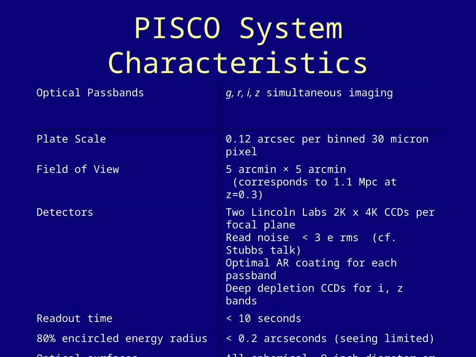
PISCO System Characteristics

Optical Passbands g, r, i, z simultaneous imaging

Plate Scale 0.12 arcsec per binned 30 micron pixel

Field of View 5 arcmin × 5 arcmin (corresponds to 1.1 Mpc at z=0.3)

Detectors Two Lincoln Labs 2K x 4K CCDs per focal planeRead noise < 3 e rms (cf. Stubbs talk)Optimal AR coating for each passbandDeep depletion CCDs for i, z bands

Readout time < 10 seconds

80% encircled energy radius < 0.2 arcseconds (seeing limited)

Optical surfaces All spherical, 9 inch diameter or smaller lenses.

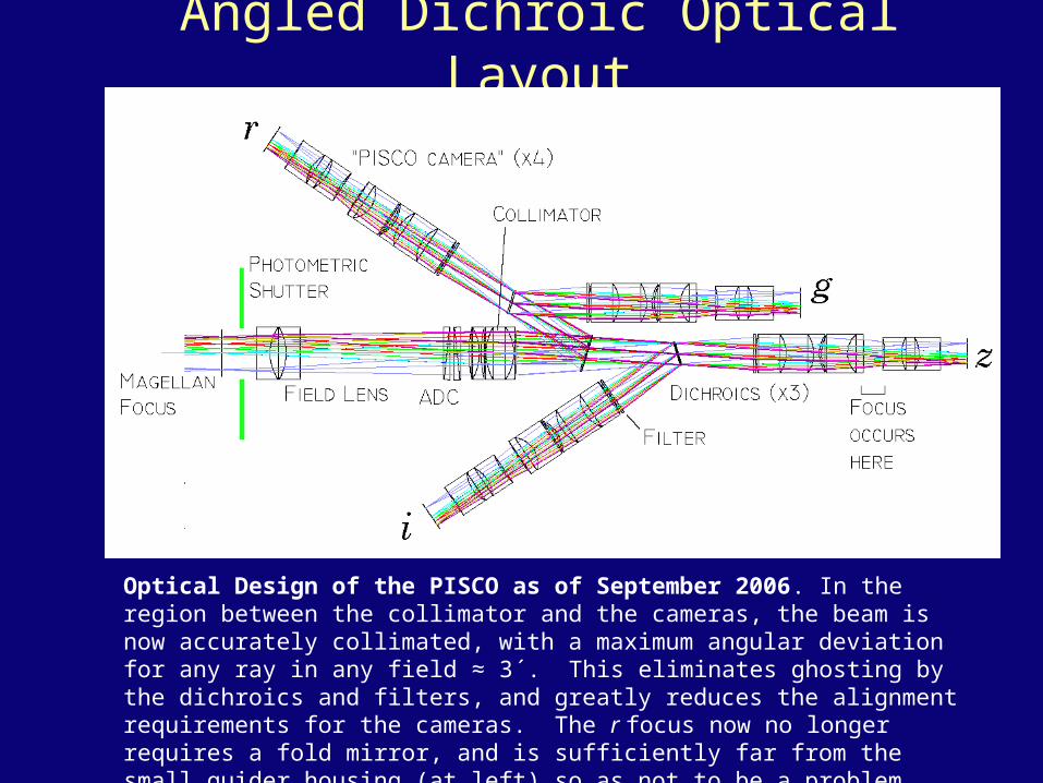
Angled Dichroic Optical Layout

Optical Design of the PISCO as of September 2006. In the region between the collimator and the cameras, the beam is now accurately collimated, with a maximum angular deviation for any ray in any field ≈ 3´. This eliminates ghosting by the dichroics and filters, and greatly reduces the alignment requirements for the cameras. The r focus now no longer requires a fold mirror, and is sufficiently far from the small guider housing (at left) so as not to be a problem (check this with F. Perez!). Focus is now telecentric.

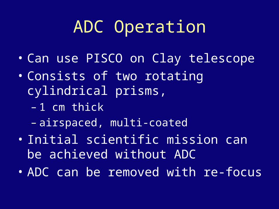
ADC Operation

• Can use PISCO on Clay telescope

• Consists of two rotating cylindrical prisms, – 1 cm thick– airspaced, multi-coated

• Initial scientific mission can be achieved without ADC

• ADC can be removed with re-focus

Dichroic in Cube Optical Layout

Alternate Optical Design of PISCO. The dichroics are embedded into cubes of fused silica, so that there is no difference in dielectric constant on either side of the dichroic. This allows the dichroics to be used at 45º. The dichroics are placed in the telecentric beam from the focal reducer, so all field positions have identical ranges of angle of incidence at the dichroics. The overall length of the instrument is reduced to 1.6 meters, and all CCDs are in a single, medium-sized dewar.

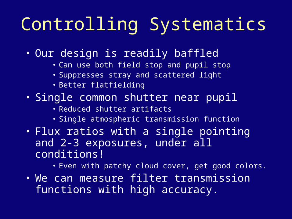
Controlling Systematics

• Our design is readily baffled• Can use both field stop and pupil stop• Suppresses stray and scattered light• Better flatfielding

• Single common shutter near pupil• Reduced shutter artifacts• Single atmospheric transmission function

• Flux ratios with a single pointing and 2-3 exposures, under all conditions!

• Even with patchy cloud cover, get good colors.

• We can measure filter transmission functions with high accuracy.

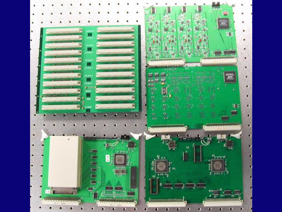
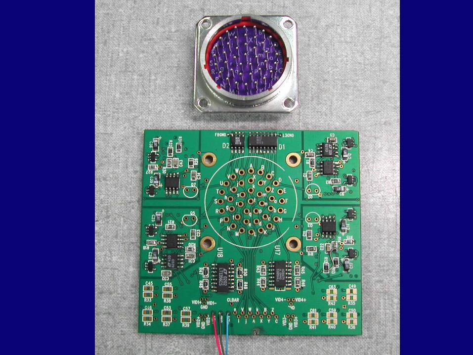
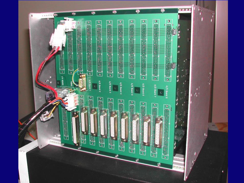
Electronics are done…

• We have already taken images in the lab with full control-to-image software.

• Readout noise is OK (3 electrons).

• Readout speed is OK ( < 8 seconds).

Initial detector tests look favorable

Tested 2 3K x 6K 10 micron high-rho devices in Univ of Hawaii test system.

Read noise

Dark current vs. temperature

CTE via Fe55 xrays

Gain via Fe55 xrays

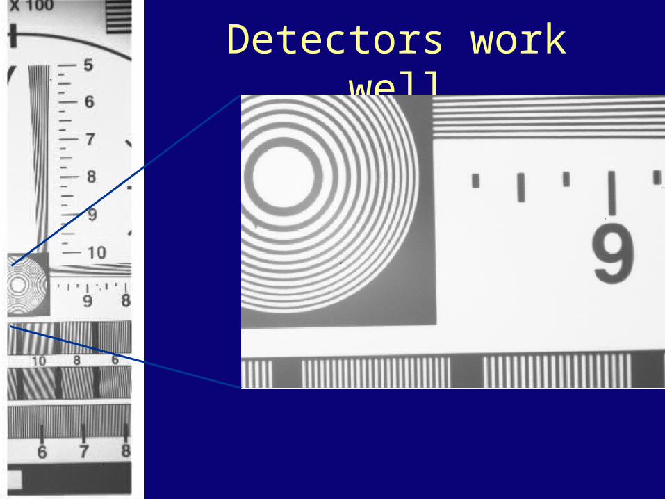
Detectors work well

Analysis Software: We’ll build upon SuperMacho/ESSENCE image analysis

pipeline

Battle tested over past 6 years at CTIO for SM and ESSENCE surveys.– Flatten with dome flats, fringe flat and sky flats

– Astrometric WCS registration, warp to fixed plate scale

– Photometry to 1%

– CVS code management, easy to add new modules

– Parallel implementation, Condor on Linux boxes

– Robust and self-tracking

– Honed on crowded fields

– Need to add (1) cluster photo-z module, and (2) SQL database

– Armin Rest, pipemeister, coming to CfA in Spring 2007.

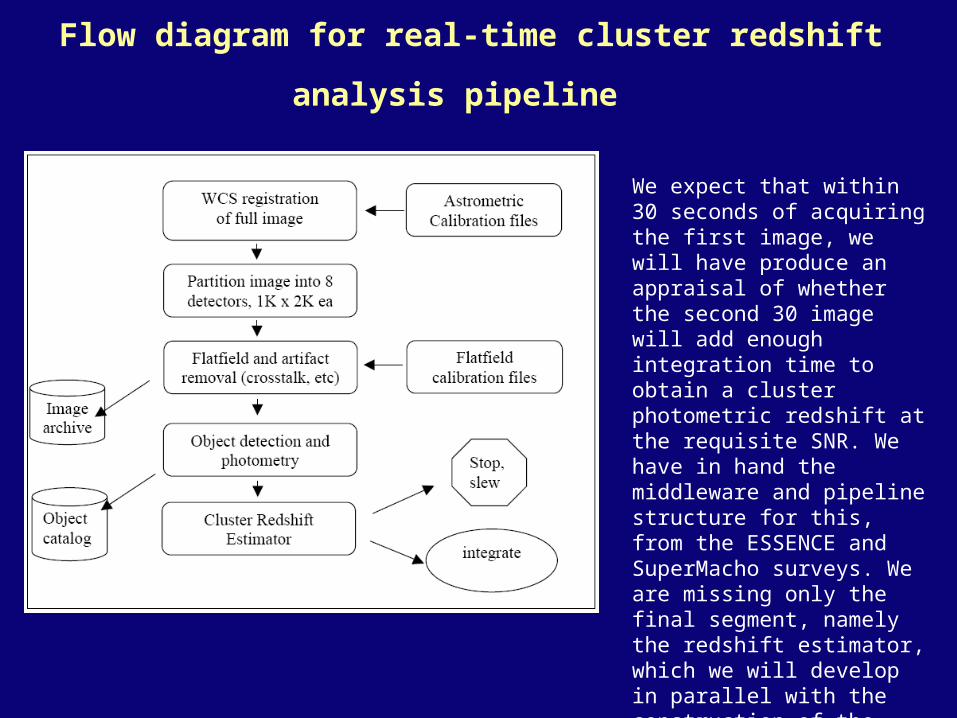
Flow diagram for real-time cluster redshift analysis pipeline

We expect that within 30 seconds of acquiring the first image, we will have produce an appraisal of whether the second 30 image will add enough integration time to obtain a cluster photometric redshift at the requisite SNR. We have in hand the middleware and pipeline structure for this, from the ESSENCE and SuperMacho surveys. We are missing only the final segment, namely the redshift estimator, which we will develop in parallel with the construction of the hardware.

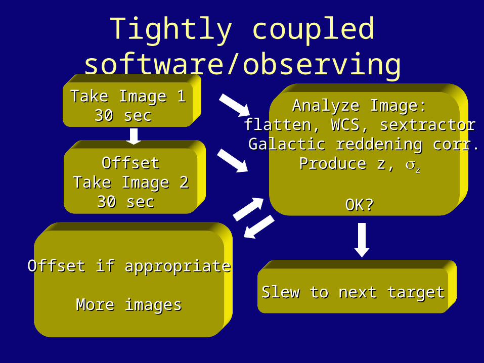
Tightly coupled software/observing

Take Image 1Take Image 130 sec 30 sec

Analyze Image: Analyze Image: flatten, WCS, sextractor flatten, WCS, sextractor Galactic reddening corr.Galactic reddening corr.

Produce z, Produce z, zz

OK? OK?

OffsetOffsetTake Image 2Take Image 2

30 sec 30 sec

Slew to next targetSlew to next target

Offset if appropriateOffset if appropriate

More imagesMore images

Photometric Redshift PrincipleThe plots show how the observer-frame spectrum of an early-type galaxy depends upon its redshift. The redshifts are indicated in the upper left corner of each panel. The flux ratios between the g, r, i, and z bands is a good indicator of galaxy redshift, as the 4000 Å break moves across the spectrum. We will develop real-time analysis code that will produce an initial cluster redshift result within 30 seconds of the acquisition of an image.

Photometric Redshift for Clusters

• Photo-z’s for individual galaxies tend to have scatter of z/(1+z)~0.03, but with a few “catastrophic” outliers.

• Combination of morphology, magnitude, color and location can be used to establish cluster’s redshift.

• Robust statistics can be used to eliminate “outliers”.

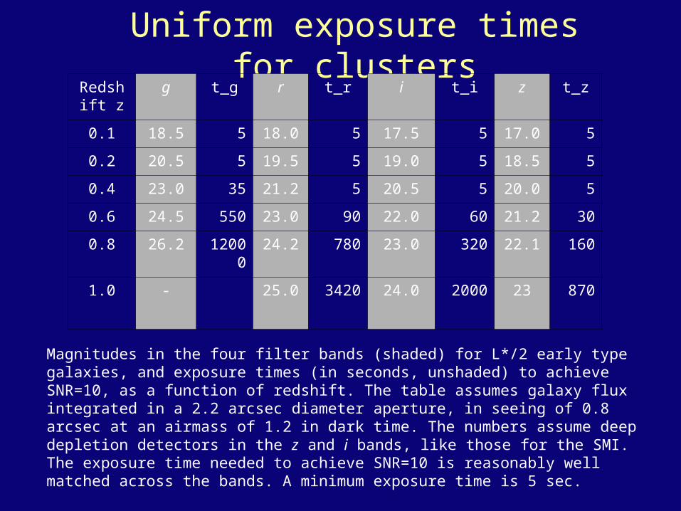
Uniform exposure times for clustersRedshif

t zg t_g r t_r i t_i z t_z

0.1 18.5 5 18.0 5 17.5 5 17.0 5

0.2 20.5 5 19.5 5 19.0 5 18.5 5

0.4 23.0 35 21.2 5 20.5 5 20.0 5

0.6 24.5 550 23.0 90 22.0 60 21.2 30

0.8 26.2 12000 24.2 780 23.0 320 22.1 160

1.0 - 25.0 3420 24.0 2000 23 870

Magnitudes in the four filter bands (shaded) for L*/2 early type galaxies, and exposure times (in seconds, unshaded) to achieve SNR=10, as a function of redshift. The table assumes galaxy flux integrated in a 2.2 arcsec diameter aperture, in seeing of 0.8 arcsec at an airmass of 1.2 in dark time. The numbers assume deep depletion detectors in the z and i bands, like those for the SMI. The exposure time needed to achieve SNR=10 is reasonably well matched across the bands. A minimum exposure time is 5 sec.

One night to obtain 115 cluster redshifts at z < 1.5 z range N clusters N * exposure time (seconds)

0.0 – 0.2 15 15 * 60 = 900

0.2 – 0.4 30 30 * 60 = 1800

0.4 – 0.6 30 30 * 60 = 1800

0.6 – 0.8 15 15 * 200 = 3000

0.8 – 1.0 10 10 * 800 = 8000

1.0 – 1.2 9

1.2 – 1.4 4 15 * 1000 = 15000

1.4 – 1.6 2

Totals 4 hours for 100 clusters to z=14.2 add’l hrs for 15 at z > 1

The time needed to obtain 115 cluster redshifts, in good conditions, is 8.2 hours. It will not be possible to obtain redshifts for the ~10% of clusters with redshift z > 1.5; these will be flagged to obtain redshifts using other instruments.

Abell 267, extrapolated to various redshiftsand observed with PISCO

Order of detection by PISCO

8 bright red galaxies detected first (green circles)

Black-circled detected next

Blue dots are cluster galaxies

Black dots are foreground

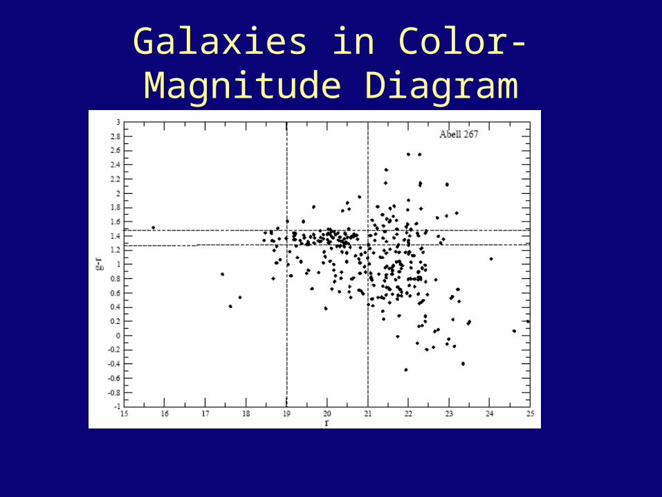
Galaxies in Color-Magnitude Diagram

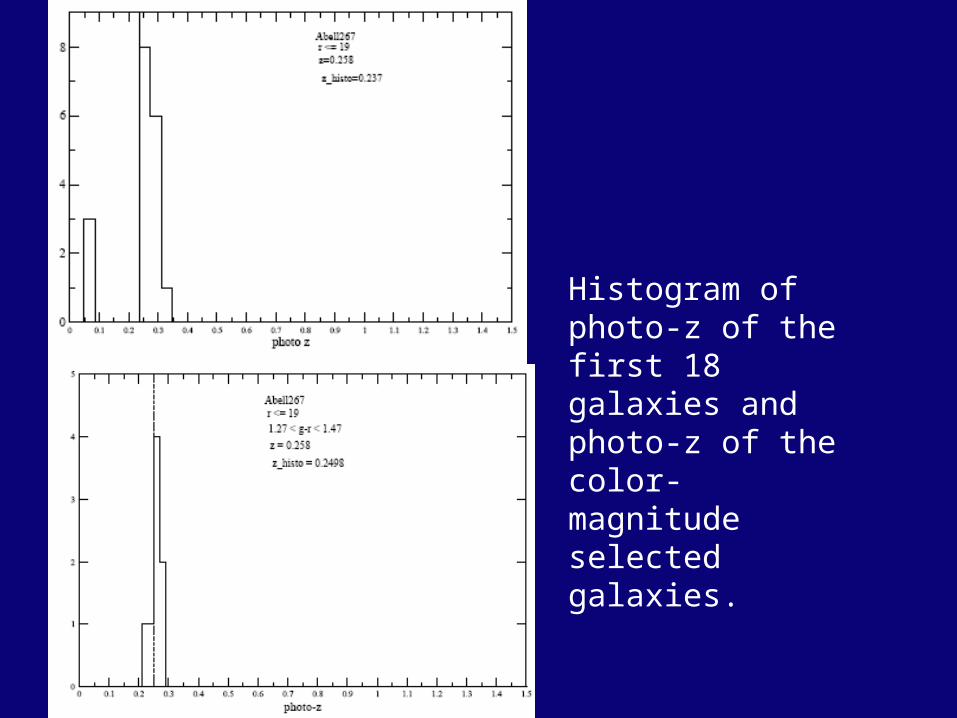
Histogram of photo-z of the first 18 galaxies and photo-z of the color-magnitude selected galaxies.

Science Opportunities• Supernova followup observations

• Type Ia and type II Sne as cosmological probes• Requires multiband images, multiple epochs

• Photometric redshifts of clusters• 4 band imaging over 5 arcmin field

• Transient followup• Evolution of SED for GRBs• Microlensing light curves

• Planetary occultations• Multiband data useful for discrimination

• Followup camera for PanSTARRS/LSST

Masses and radii of transiting extrasolar planets

The dashed lines correspond to loci of constant mean density. The symbols indicate the nine known transiting planets, along with Jupiter and Saturn. Two symbols are shown for OGLE-TR-10b. In green is the result based on a fit to the OGLE photometry and available radial velocities (Konacki et al. 2005). In blue is the Holman et al. (2005) result, based on a simultaneous fit to Magellan photometry and the same radial velocity measurements.

Project timeline Major Review of Hardware Design 12/13/06

Optical System Design Completed 1/30/07 (but…new idea)

Optics Delivery 10/15/07

Software design complete 10/1/07

Finish assembly of all hardware subsystems 12/1/07

Software complete, integrated 1/1/08

Full integration on lab bench 2/1/08

Target shipping date 2/08

Shakedown run on Magellan 3/08

First SPT cluster observations 3/08

The construction of our instrument is timed to allow us to be ready for pipelined observations of SPT-SZ clusters in early 2008.

PISCO Current Status

• Some observing time granted in 4th quarter 2007 for photo-z observations of clusters– What should we observe? Need to know soon.

• Funds are available from Smithsonian to complete PISCO construction

• Successfully obtained private foundation grant for a PostDoc

• Proposals pending at NSF, DOE for ongoing support

Australia Telescope Compact Array (ATCA) observations of SPT clusters

                                                 

Antony Stark Antony Stark Smithsonian Astro ObsSmithsonian Astro Obs

Wilfred WalshWilfred Walsh U. New South Wales Asia U. New South Wales Asia

Joe MohrJoe Mohr U. IllinoisU. Illinois

Tom CrawfordTom Crawford U. ChicagoU. Chicago

Antony Stark Antony Stark Smithsonian Astro ObsSmithsonian Astro Obs

Wilfred WalshWilfred Walsh U. New South Wales Asia U. New South Wales Asia

Joe MohrJoe Mohr U. IllinoisU. Illinois

Tom CrawfordTom Crawford U. ChicagoU. Chicago

Relevance to SPT Cluster Survey

• SPT system is around 100 Jy/K• SPT-SZ survey will be 10 μK rms per beam• Point continuum sources that are 1 mJy or brighter

will make a significant contribution to the data, and possibly affect the detection of clusters and their derived parameters.

• The number of such sources in SPT bands is poorly known.

• With the ATCA, we can actually search for and detect such sources in SPT clusters.

Pilot Study Completed

• We were actually awarded a significant amount of observing time on ATCA

• “Extragalactic” time slot is undersubscribed, and not too hard to get observing time

• We observed 24 X-ray selected moderate redshift clusters (Mullis et al. 2003) in redshift range 0.05 < z < 0.65

• Observe at 18 GHz, because of ATCA sensitivity and map area; possible follow-up at 90 GHz

• Detected one source at ~ 2 mJy at 18 GHz• Our sensitivity was primarily limited by phase stability—we

will need good weather

Current Status

• Proposal in to NSF AST for travel and publication expenses—no decision yet.

• Additional proposals submitted for observing time.

THE ENDhttp://www.tonystark.org