Pinned fronts in heterogeneous media of jump typemath.bu.edu/people/heijster/PAPERS/HETEROGENEOUS.pdf · Pinned fronts in heterogeneous media of jump type 129 0 ... three are needed

Pinned fronts in heterogeneous media of jump type

This article has been downloaded from IOPscience. Please scroll down to see the full text article.

2011 Nonlinearity 24 127

(http://iopscience.iop.org/0951-7715/24/1/007)

Download details:

IP Address: 128.148.84.78

The article was downloaded on 29/11/2010 at 14:52

Please note that terms and conditions apply.

View the table of contents for this issue, or go to the journal homepage for more

Home Search Collections Journals About Contact us My IOPscience

http://iopscience.iop.org/page/terms

http://iopscience.iop.org/0951-7715/24/1

http://iopscience.iop.org/0951-7715

http://iopscience.iop.org/

http://iopscience.iop.org/search

http://iopscience.iop.org/collections

http://iopscience.iop.org/journals

http://iopscience.iop.org/page/aboutioppublishing

http://iopscience.iop.org/contact

http://iopscience.iop.org/myiopscience

IOP PUBLISHING NONLINEARITY

Nonlinearity 24 (2011) 127–157 doi:10.1088/0951-7715/24/1/007

Pinned fronts in heterogeneous media of jump type

Peter van Heijster1, Arjen Doelman2, Tasso J Kaper3,Yasumasa Nishiura4 and Kei-Ichi Ueda5

1 Division of Applied Mathematics, Brown University, 182 George Street, Providence,RI 02912, USA2 Mathematisch Instituut, Universiteit Leiden, PO Box 9512, 2300 RA Leiden, Netherlands3 Department of Mathematics and Center for BioDynamics, Boston University, 111 CummingtonStreet, Boston, MA 02215, USA4 Laboratory of Nonlinear Studies and Computation, Research Institute for Electronic Science,Hokkaido University, Sapporo 060-0812, Japan5 Research Institute for Mathematical Sciences, Kyoto University, Kyoto 606-8502, Japan

Received 11 June 2010, in final form 2 November 2010Published 25 November 2010Online at stacks.iop.org/Non/24/127

Recommended by J Lega

AbstractIn this paper, we analyse the impact of a (small) heterogeneity of jump typeon the most simple localized solutions of a 3-component FitzHugh–Nagumo-type system. We show that the heterogeneity can pin a 1-front solution,which travels with constant (non-zero) speed in the homogeneous setting, toa fixed, explicitly determined, distance from the heterogeneity. Moreover,we establish the stability of this heterogeneous pinned 1-front solution. Inaddition, we analyse the pinning of 1-pulse, or 2-front, solutions. Thepaper is concluded with simulations in which we consider the dynamics andinteractions of N -front patterns in domains with M heterogeneities of jump type(N = 3, 4, M � 1).

Mathematics Subject Classification: 35K57, 35K45, 35B36, 35B25, 35Q92

1. Introduction

In many (classical) mathematical models, especially those of reaction–diffusion type, themedium in which the process under consideration takes place is (implicitly) assumed to behomogeneous. This is of course a simplification; natural media, even in their equilibriumstates or background states, generally contain heterogeneities. For instance in the field ofsuperconductivity, there is quite an extensive literature, dating back to the 1970s, on the impactof spatially localized heterogeneities, or ‘impurities’, on the dynamics of localized structures(the so-called fluxons), see [14]. There is also a special interest in the influence of spatial

0951-7715/11/010127+31$33.00 © 2011 IOP Publishing Ltd & London Mathematical Society Printed in the UK & the USA 127

http://dx.doi.org/10.1088/0951-7715/24/1/007

http://stacks.iop.org/no/24/127

128 P van Heijster et al

heterogeneities on the dynamics of localized structures such as fronts and pulses in reaction–diffusion equations, see [1, 2, 16, 18, 24, 25] and references therein. The pinning phenomenon,in which a travelling solution gets trapped by the heterogeneity while its homogeneousequivalent would have kept on travelling, can be considered as one of its most dramaticeffects.

While pinning has been studied analytically in the special case of scalar equations(see [2, 24] and references therein), it has been studied much less extensively for systemsof reaction–diffusion equations [9–11], see remark 1.1. Numerically, pinning for systems ofreaction–diffusion equations has been studied more thoroughly. A model for which extensivenumerical simulations are available is a generalized FitzHugh–Nagumo-type (FHN) system.This model has been proposed to describe, on a phenomenological level, the behaviour of gas-discharge systems, see [19, 20] and references therein. In two space dimensions this system isgiven by

Ut = DU�U + f (U) − κ3V − κ4W + κ1(x, y),

τVt = DV �V + U − V,

θWt = DW�W + U − W,

(1.1)

where f (U) is typically a cubic nonlinearity and κ1(x, y) models the heterogeneity. System(1.1) is also a natural extension of the FHN equations to systems with two inhibitors. Since(1.1) is a system, the pinning phenomenon cannot be studied by the methods employed in [2],which rely heavily on the scalar nature of the equations under consideration. For instance,scalar systems have a gradient structure, and their solutions can be controlled by sub- and super-solutions. These properties are crucial ingredients in the analysis of [2]. Moreover, unlikethe models used for pinning in superconductivity, (1.1) is not close to a completely integrablepartial differential equation (PDE), so that the impact of (localized, spatial) heterogeneitiescannot be studied by a perturbation method based on this fact [14]. In this paper, we employa dynamical systems approach to analyse the impact of localized heterogeneities on localizedsolutions of (1.1). Note that this approach is similar to that of [1] which considers a model forJosephson junctions with jump type heterogeneities.

In [25], the influence of a small smoothened jump type heterogeneity on travelling pulsesof (1.1) in one space dimension is studied. It is observed that a travelling pulse collidingwith the heterogeneity can penetrate, be annihilated, rebound, oscillate or get pinned. Moreprecisely, the pinned solutions are observed when the heterogeneity jumps down, and thepinned solutions are ‘in front’ of the heterogeneity, that is, they are located immediately to theleft of the heterogeneity. In [18], the influences of two different heterogeneities on travellingpulses are investigated for the same model, that is, the influences of a symmetric bump type, or2-jump, heterogeneity and a periodic heterogeneity are studied. For the bump heterogeneity,also penetration, rebound, annihilation, oscillation and pinning are observed. However, thereare now two types of pinned solutions. One is a pinned solution ‘in front’ of a bump, andthe other one is a pinned solution in the bump region. The pinned solution which is observeddepends on the bump being up or down. For the periodic heterogeneity, also spatio-temporalchaos is observed.

In this paper, we present an analytic understanding of the pinning phenomenon inheterogeneous media. That is, we develop a method by which it is possible to predict forwhich parameter values pinning can be expected. We will focus on the most elementary(localized) solutions, that is, the 1-front solutions and 2-front (or 1-pulse) solutions, and wewill also use these insights to study more extended patterns. Motivated by the numericalsimulations discussed in the previous paragraph, we analyse the pinning phenomenon in the

Pinned fronts in heterogeneous media of jump type 129

0

0.5

1

1.5

2

2.5

3

-1000

-500

0

500

1000

-1

0

1

0

0.5

1

1.5

2

2.5

3

-1000

-500

0

500

1000

-1

0

1

0

0.5

1

1.5

2

2.5

3

-1000

-500

0

500

1000

-1

0

1

Figure 1. A travelling front solution of (1.2) that asymptotes to a stationary front, located at theheterogeneity, and hence is said to be pinned there. The system parameters are chosen as follows(α, β, γ1, γ2, τ, θ, D, ε) = (3, 1, 1, −3, 1, 1, 5, 0.01). The thick black dashed line indicates thelocation of the heterogeneity.

3-component FHN system (1.1) in a particular scaling

Ut = Uξξ + U − U 3 − ε(αV + βW + γ (ξ)),

τVt = 1

ε2Vξξ + U − V,

θWt = D2

ε2Wξξ + U − W,

(1.2)

with 0 < ε � 1; D > 1; τ, θ > 0; (x, t) ∈ R × R+; α, β ∈ R,

γ (ξ) ={

γ1 for ξ < 0,

γ2 for ξ � 0,(1.3)

with γ1,2 ∈ R\{0}, see remark 1.2. Here, all parameters are assumed to be O(1) with respectto ε. This typical scaling of (1.1) has been introduced in [5]. See figure 1 for a pinned 1-frontsolution.

We choose this particular heterogeneous model since it is sufficiently transparent forthe purposes of performing explicit mathematical analysis, while at the same time it issufficiently complex to support complex localized structures. More specifically, our results(and analysis) simplify in the special cases when either α = 0 or β = 0. These correspondto reductions of the 3-component model to a simpler 2-component model. In particular,our results (theorems 1.4 and 1.5) show that also the 2-component model exhibits pinnedfront and 2-front solutions. However, as will be clear later on, the dynamics of the 2-frontsolutions (and more general N -front solutions) are much richer in the 3-component model, seealso [5, 21]. Moreover, to analyse scattering and other more complex phenomena observedin [17], the analysis developed here for the full 3-component model will be required. Also,as is clear from the above discussion, this model has been extensively studied via numericalsimulations. The specific choice of the heterogeneity comes, on the one hand, from the jumptype heterogeneity considered in [25]. On the other hand, it is motivated by our intention tokeep the analysis manageable. Furthermore, a (smoothened) step function can be seen as abasic ingredient for more general heterogeneities such as periodic and random media [25].By the choices we made, we are able, for example, to explicitly determine the pinningdistance of the localized structures to the heterogeneity and how that depends on the systemparameters.

In [5, 22, 21], a detailed analysis of the existence [5], stability [21] and interaction [22] oflocalized structures for the homogeneous problem ((1.2) with γ (ξ) ≡ γ , constant) is given.


Of the main results of these papers, three are needed for this paper:

Theorem 1.1 ([22]). For ε > 0 small enough, the homogeneous model ((1.2) with γ (ξ) ≡ γ ,constant) possesses a stable travelling 1-front solution which travels with speed 3

2

√2εγ ; it

possesses no stationary 1-front solutions.

Theorem 1.2 ([22]). For ε > 0 small enough, the width � of a 2-front solution to thehomogeneous model evolves according to

�(t) = 3√

2ε(αe−ε� + βe− εD

� − γ ), (1.4)

where � := 2 − 1, with i the ith intersection of the Ucomponent with zero.

Theorem 1.3 ([5, 21]). For ε > 0 small enough, the homogeneous model possesses a1-parameter family of stationary 2-front, or 1-pulse, solutions with width ξ

γ

hom > 0, if there isa ξ

γ

hom solving

αe−εξγ

hom + βe− εD

ξγ

hom = γ. (1.5)

This solution is stable if

αe−εξγ

hom +β

De− ε

Dξ

γ

hom > 0.

Note that the stationary solutions (1.5) with � = ξγ

hom are the fixed points of (1.4).There are several important differences between the heterogeneous system (1.2) and its

homogeneous equivalent (γ (ξ) ≡ γ ). First, due to the discontinuity in γ (ξ) at ξ = 0, wecannot expect the solutions to the PDE to be smooth. More precisely, due to the heterogeneitythe solutions can only be C0 in time and C1 in space. Since we are interested in stationarysolutions, we can rewrite (1.2) into a six-dimensional system of ordinary differential equations(ODEs), see for example (2.2). The solutions to these resulting systems will only be C0 (inspace).

The second, and most important, difference is that the heterogeneous model is no longertranslation invariant. This loss of translation invariance challenges the methods developedin [5, 21] in which the existence and stability of localized homogeneous structures wasstudied. By this loss, the spatial derivative of the localized stationary structure is no longeran eigenfunction of the linearized stability problem with corresponding eigenvalue zero, sincethis derivative is only C0 and not C1. This has two consequences for the stability analysis.First, we have to determine in which fashion this zero eigenvalue perturbs, since it will yieldan instability if it moves into the right half plane. Second, in [21] the translation invariancewas used to derive an extra solvability condition from the existence analysis that was used as acrucial ingredient in the stability analysis. Therefore, we have to find a new way to determinethe heterogeneous equivalent of this solvability condition.

A third difference is that for the heterogeneous system it is a priori not clear what the‘trivial’ background solutions are, see also remark 1.2. However, their asymptotic behaviourcan be determined. As ξ → ±∞, the background solutions limit on

(U, V, W) = u±γi(1, 1, 1), with u±

γi= ±1 ∓ 1

2ε(α + β ± γi) + O(ε2), i = 1, 2, (1.6)

or

(U, V, W) = u0γi(1, 1, 1), with u0

γi= εγi + O(ε2), i = 1, 2, (1.7)

see also [5]. Note that u±,0γi

are precisely the solutions to the cubic polynomial

u − u3 − ε(αu + βw + γi), i = 1, 2.

Since the O(ε) solution (1.7) is unstable it will not be considered in this paper.


Figure 2. Heuristically, we expect pinning of a 1-front solution if γ1 > 0 > γ2. That is, weexpect pinning in frame II. Note that only (the singular limit of) the U component of the front isdepicted.

System (1.2) has two important symmetries

(U, V, W, γ1, γ2) → (−U, −V, −W, −γ1, −γ2) (1.8)

and

(ξ, γ1, γ2) → (−ξ, γ2, γ1). (1.9)

The first symmetry allows us to restrict to solutions which asymptote to u−γ1

(1, 1, 1) asξ → −∞. For example, we construct stable pinned 1-front solutions which asymptote tou−

γ1(1, 1, 1). By the first symmetry, we then immediately obtain a stability condition for

pinned 1-front solutions which asymptote to u+−γ1

(1, 1, 1) as ξ → −∞. The second symmetryallows us to obtain additional results for the mirrored solution by interchanging the role of γ1

and γ2. For example, from the existence condition for a 2-front solution with its front pinned atthe heterogeneity, we obtain the existence condition for a 2-front solution with its back pinnedat the heterogeneity by interchanging γ1 and γ2. Therefore, without loss of generality we canrestrict the numerical simulations to γ1 > γ2 as we did in section 4.1.

This paper is organized as follows. In the next two sections, we establish the conditionsunder which the heterogeneity pins a travelling 1-front solution, and explicitly determine itsdistance from the heterogeneity. We recall from theorem 1.1 that stationary 1-front solutionsdo not exist for the homogeneous problem (γ �= 0, see remark 1.2). The main pinningresult is

Theorem 1.4. For ε > 0 small enough, there exists a stable pinned 1-front solution whichasymptotes to (U, V, W) = u−

γ1(1, 1, 1) as ξ → −∞ and whose front is pinned near the

heterogeneity if and only if γ2 < 0 < γ1.

See theorems 2.1 and 3.1 for a more detailed formulation of this result. Intuitively, thistheorem can be explained from the results on travelling 1-front solutions in the homogeneoussystem, see theorem 1.1. These 1-front solutions (which asymptote to (U, V, W) = u−

γ1(1, 1, 1)

as ξ → −∞) travel in the direction of the sign of γ . So, fronts travel to the right if γ is positiveand to the left if γ is negative. Therefore, we expect pinning for the heterogeneous model at theheterogeneity if, and only if, γ1 is positive and γ2 is negative. Under these conditions, a 1-frontsolution away from the heterogeneity always moves towards it. All the other configurationsof γ1 and γ2 yield movement of the front towards infinity. See also figure 2.

In section 4, we determine the existence condition for stationary 2-front solutions whosefront is pinned near the heterogeneity, where we recall that a 2-front solution consists of a front


(positive derivatives) concatenated to the right with a back (negative derivatives). Again, weare able to explicitly compute pinning distance. The main result is

Theorem 1.5. For ε > 0 small enough and γ1 > γ2, there exists a pinned 2-front solutionwhich asymptotes to (U, V, W) = u−

γ1(1, 1, 1) as ξ → −∞ and whose front is located near

the heterogeneity if and only if there exists a ξ2f > 0 solving

αe−εξ2f + βe− εD

ξ2f = γ2. (1.10)

Moreover, the width of the 2-front solution is ξ2f .

See theorem 4.1 for a more detailed formulation of this result. Note that condition (1.10)coincides with the existence condition of a stationary 2-front solution in the homogeneous casewith γ = γ2, see theorem 1.3. Also observe the different role of the heterogeneity betweenthe pinning of the 1-front solution and the pinning of the 2-front solution. The heterogeneity‘creates’ a new stationary 1-front solution, while it ‘selects’ a particular stationary 2-frontsolution from a 1-parameter family, see theorems 1.1 and 1.3. Moreover, theorem 1.5 confirmsthe numerical observations of pinned pulses in front of a heterogeneity which jumps down [25](note the sign difference in front of κ1(x, y) and γ (ξ)). In this paper, we have refrained fromexplicitly determining the stability of this type of 2-front solution, especially since the pinningdistance is not O(1), but O(| log ε|), see theorem 4.1. Therefore, determining the stability is avery technical procedure that, in principle, can be done with the methods discussed in section 3of this paper and in [21].

In the last section, we present numerical results on N -front solutions with N = 3, 4, frontsolutions for different heterogeneities and travelling 2-front solutions (τ large).

Remark 1.1. Note that (1.2) differs substantially from the model studied in [9–11]. In thesepapers, the authors analyse the influence of a spatial heterogeneity in the diffusion coefficientson the solutions to a specific bistable two-component reaction–diffusion system. In this paper,the spatial heterogeneity is encoded in the reaction term and (1.2) has three components.Moreover, [9–11] focus entirely on front solutions. In [9] pinning, rebound and penetrationphenomena are studied in a system that is assumed to be close to a drift bifurcation, i.e. thebifurcation at which a travelling front bifurcates from the standing front. The analysis is basedon a centre manifold approach that has been developed to describe the weak interactions offronts [6]. From the analytical point of view, the main differences between the present workand [9–11] is that (i) we use geometrical singular perturbation theory to explicitly constructthe leading order profile of 1-front and 1-pulse, or 2-front, solutions and determine explicitstability conditions (in a 3-component model), see theorems 2.1, 3.1 and 4.1; (ii) our methodsenable us to go beyond the setting of weak interactions and thus to consider N -front patterns(N > 1) that interact in a semi-strong fashion [3, 22], see also section 5.

Remark 1.2. In this paper, we only analyse the interaction of the jump heterogeneity through afast field of a localized pattern. That is, we only consider patterns that have one of their frontslocated near the heterogeneity. We do not analyse the influence of the jump heterogeneitythrough the slow fields. That is, we do not analyse stationary front solutions which arean O(ε−1/2), or more, distance away from the heterogeneity. The numerical simulations insection 4 indicate that these types of pinned solutions exist for 2-front solutions, see figures 4and 5. Moreover, the distance between the pinned front and the heterogeneity diverges as eitherγ1 or γ2 → 0, see (2.1) in theorem 2.1. This is related to the fact that the homogeneous problempossesses a 1-parameter family of stationary 1-front solutions for γ = 0. Thus, as γi ↓ 0,the front cannot be considered to be close to the heterogeneity. Therefore, we imposed thatγi is not equal to zero. This way, we make sure that we exclude this type of weak interaction


for 1-front solutions. Also observe that we do not construct the background solutions, calleddefect solutions in [25], which can be seen as heteroclinic connections between u−

γ1(1, 1, 1) and

u−γ2

(1, 1, 1) that remain uniformly O(ε) close to (−1, −1, −1): these solutions also interactweakly with the heterogeneity. These weak interactions through the slow fields are the subjectof upcoming research.

Remark 1.3. The analysis in this paper can be extended to the case in which stripe solutions ofequation (1.2) are studied on a bounded strip in the plane, that is, (x, y) ∈ R× [0, L]. For suchsolutions, one can carry out a modal decomposition in terms of the vertical wave number andthen employ the one-dimensional analysis used here, incorporating the vertical wave numberas a parameter. We refer to [4], where such a decomposition and analysis is performed forstripe solutions in the two-dimensional Gierer–Meinhardt model. The interaction with spatialinhomogeneities can also be studied along these lines if the inhomogeneity also is a jumpheterogeneity with a vertical structure, that is, if γ (ξ1, η1) = γ (ξ1).

A more challenging extension to studying (1.2) in two dimensions involves examining spotsolutions, which are analogues of 2-front solutions in two space dimensions. In this regard, weobserve that the influence of a jump heterogeneity with a vertical structure on spot solutions of(1.1) in two space dimensions has been investigated in [26]. Based on numerical simulations,the spot can, for example, be attracted to the heterogeneity, and then transported along it. Inaddition to these numerical results, there has been some recent analysis of spot solutions inthe homogeneous two-dimensional version of (1.2). In particular, in [23], the existence andstability of stationary radially symmetric spots are examined. It is our intention to extend theanalysis in [23] to spots in the presence of heterogeneities.

2. Existence of pinned 1-front solutions

In this section, we construct pinned 1-front solutions whose fronts are located near theheterogeneity, that is, near ξ = 0.

Theorem 2.1. For each D > 1,τ, θ > 0, α, β ∈ R, γ1,2 ∈ R\{0}, and for each ε > 0small enough, there exists a unique pinned 1-front solution �f(ξ) which asymptotes to(U, V, W) = u−

γ1(1, 1, 1) (1.6) as ξ → −∞ if and only if sgn(γ1) �= sgn(γ2). Moreover,

the distance ξ ∗ (U(ξ ∗)=0) from the front to the heterogeneity is, to leading order, given by

ξ ∗ =√

2arctanh

(γ1 + γ2

γ1 − γ2

). (2.1)

This theorem establishes the existence part of theorem 1.4. (The stability part will be given bytheorem 3.1 in the next section.) Also, this theorem combined with symmetry (1.8) immediatelyyields the existence of pinned 1-front solutions which asymptote to (U, V, W) = u+

−γ1(1, 1, 1)

as ξ → −∞, under the same condition sgn(γ1) �= sgn(γ2).There are also a couple of special cases. First, if γ1 = −γ2, the heterogeneity is symmetric,

and we obtain ξ ∗ = 0. Hence, as expected in this special case, the heterogeneity and thelocation where U crosses zero coincide. Second, the asymptotics of (2.1) yields

limγ1→0

ξ ∗ = −∞, limγ2→0

ξ ∗ = ∞.

Thus, for decreasing |γi |, the location of the front goes to the left (right, respectively) boundaryof the fast field If and will eventually move out of the fast field If as |γi | becomes too small.See also remarks 1.2 and 3.1.

Proof of theorem 2.1. The method used in [5] to construct stationary pulse solutions of thehomogeneous system may be adapted to analyse stationary fronts of (1.2). First, we define


ξ ∗ as the unique value of ξ where the U component crosses zero, that is, U(ξ ∗) = 0. Notethat for the homogeneous problem, this point was not uniquely determined by the translationinvariance property. Next, we introduce the fast and slow fields

I−s :=

(−∞, − 1√

ε+ ξ ∗

), If :=

[− 1√

ε+ ξ ∗,

1√ε

+ ξ ∗]

, I +s :=

(1√ε

+ ξ ∗, ∞)

.

These three domains correspond to the slow, fast and slow regimes observed in the solutiondynamics, and in this proof we will analyse the dynamics separately in these domains.

Since we look for a pinned stationary solution, we can write the heterogeneous problem(1.2) as a singularly perturbed six-dimensional system of first-order ODEs by introducing(p, q, r) = (uξ , vξ /ε, Dwξ/ε):

uξ = p,

pξ = −u + u3 + ε(αv + βw + γ (ξ)),

vξ = εq,

qξ = ε(v − u),

wξ = ε

Dr,

rξ = ε

D(w − u).

(2.2)

Moreover, we know that the heterogeneity lies in the fast field If , that is, 0 ∈ If , because theheteroclinic pinned front solutions f (ξ) of (2.2) whose existence we establish have frontsthat lie O(1) close to the heterogeneity. By (1.3), we can split this non-autonomous systemof ODEs into two autonomous systems, one with γ (ξ) = γ1 on ξ ∈ (−∞, 0) and the otherone with γ (ξ) = γ2 on ξ ∈ [0, ∞). We label these two systems by (2.2)1, respectively, (2.2)2.The critical points of these systems are, in addition to the unstable one around zero, given by

(u, p, v, q, w, r) = (u±γi, 0, u±

γi, 0, u±

γi, 0), for i = 1, 2,

see (1.6). Since we construct front solutions that asymptote to (U, V, W) = uγ1(1, 1, 1) asξ → −∞, we are actually only interested in the critical points

(u, p, v, q, w, r) = (u−γ1

, 0, u−γ1

, 0, u−γ1

, 0) := P − , (2.3)

for (2.2)1, and for (2.2)2 we are only interested in

(u, p, v, q, w, r) = (u+γ2

, 0, u+γ2

, 0, u+γ2

, 0) := P + . (2.4)

These points are saddle fixed points of (2.2)1 and (2.2)2, respectively.The pinned 1-front solutions f (ξ) that we construct with respect to (2.2) will lie in the

transverse intersection of Wu(P −) and Ws(P +):

f (ξ) ⊂ Wu(P −) ∩ Ws(P +) . (2.5)

Moreover, these solutions will consist of three segments, a left slow segment on I−s , a fast

segment on If , and a right slow segment on I +s . Finally, since the front solution f (ξ) is C0

smooth (see section 1), the solutions to (2.2)1 and (2.2)2 should match at the heterogeneity,i.e. we must impose

limξ↑0

(u, p, v, q, w, r)(ξ) = limξ↓0

(u, p, v, q, w, r)(ξ) .

We begin with the fast segment. The fast reduced system (FRS) of (2.2) is obtained in the limitε → 0, {

uξ = p,

pξ = −u + u3,(2.6)


and (v, q, w, r) = (v∗, q∗, w∗, r∗) constants. It is independent of γ (ξ), therefore, this FRScoincides with the FRS of (2.2)1 and (2.2)2. Moreover, it also coincides with the FRS of theequivalent homogeneous problem. Therefore, the leading order results of the homogeneouscase apply here [5]. The FRS system is a conservative system with Hamiltonian

H(u, p) = 12

(u2 + p2

) − 14

(u4 + 1

). (2.7)

Its heteroclinic solutions are(u∓(ξ), p∓(ξ)

) =(± tanh

(12

√2ξ

), ± 1

2

√2sech2

(12

√2ξ

)). (2.8)

The heteroclinic (u−(ξ), p−(ξ)) is relevant to our analysis, since in the fast field If , the fastpart of f (ξ), i.e. the u and p components of the heteroclinic front f , will be O(ε) close to(u−(ξ − ξ ∗), p−(ξ − ξ ∗)), as was also the case in [5].

Next, we turn our attention to the slow fields. We define the manifolds M±0 by

M±0 = {(u, p, v, q, w, r) = (±1, 0, v∗, q∗, w∗, r∗)},

the unions of the saddle points of (2.6) over all possible v∗, q∗, w∗, r∗. Hence, for ε = 0, thesemanifolds are invariant and normally hyperbolic. Now, we turn to the persistence of theseslow manifolds for ε > 0 sufficiently small. The function γ (ξ) makes (2.2) non-autonomous,and hence one cannot immediately apply Fenichel theory [7, 12, 13] to (2.2). However, sinceγ (ξ) = γ1 for ξ < 0 along f (ξ), we are only interested in the persistence of M−

0 in the phasespace of (2.2)1 and Fenichel theory may be applied directly to the autonomous system (2.2)1

to yield the existence of a slow, invariant manifold M−1 that is O(ε) close to M−

0 :

M−1 := {

(u, p, v, q, w, r) | u = −1 − 12ε(αv + βw + γ1) + O(ε2), p = O(ε2)

}. (2.9)

Similarly, since γ (ξ) = γ2 for ξ > 0 along f (ξ), we are interested in the persistence of M+0

in the phase space of (2.2)2 and Fenichel theory may be applied directly to the autonomoussystem (2.2)2 to yield the existence of a slow, invariant manifold M+

2 that is O(ε) close to M+0:

M+2 := {

(u, p, v, q, w, r) | u = 1 − 12ε(αv + βw + γ2) + O(ε2), p = O(ε2)

}, (2.10)

see also [5].In the slow fields I±

s , the heteroclinic orbit f has to be exponentially close to M±1,2,

and its evolution is determined by the slow (v, q, w, r) equations [5]. These are given by theslow reduced systems (SRS) of (2.2)1 and (2.2)2, respectively. That is, near M−

1 the flow is toleading order governed by

vξξ = ε2(v + 1),

wξξ = ε2

D2(v + 1),

(2.11)

and near M+2 by

vξξ = ε2(v − 1),

wξξ = ε2

D2(v − 1).

(2.12)

These flows are independent of γ1,2, and thus the same as the homogeneous slow flows forthe equivalent homogeneous problem. The fixed points of (2.11) and (2.12) correspond tosaddle–saddle points on M±

1,2 which correspond to the background states (2.3) and (2.4),respectively.

The result of the theorem will follow by the Melnikov approach employed in [5], becausethis calculation will establish that Wu(M−

1 ) and Ws(M+2) intersect transversally. In particular,

we determine the net changes in the Hamiltonian (2.7) and the slow v, w components over thefast field If for the full perturbed system (2.2).


We start with the latter. Similar to the homogeneous case [5], the v and w componentsare constant to leading order during the jump through the fast field If . This can best be seenfrom the fact that the heterogeneity in γ has no leading order influence on the v, w equations.More precisely, by (2.2)

v = v0 + εq0(ξ − ξ ∗) + O(ε2), w = w0 +ε

Dr0(ξ − ξ ∗) + O(ε2) in If , (2.13)

with v0, q0, w0, r0 constants. Hence, on If , the slow components v and w are constant toleading order.

Next, we work with Hamiltonian (2.7). The fact that γ (ξ) is not constant does not havean effect on the values of the Hamiltonian on the slow manifolds M±

1,2:

H |M∓1,2

= − 14ε2

(αv + βw + γ1,2

)2+ O(ε3). (2.14)

We now can determine the change in the Hamiltonian over the fast field If in two ways. First,we know that f (ξ) must be exponentially close to M±

1,2 outside the fast field [5]. Thus, by(2.5) we have that H(f (ξ)) → H |M−

1for ξ → I−

s and H(f (ξ)) → H |M+2

for ξ → I +s .

Therefore,

�f H = H |M+2− H |M−

1= − 1

4ε2(γ2 − γ1)(2αv0 + 2βw0 + γ2 + γ1) + O(ε2√ε), (2.15)

where we have used that the slow components are constant to leading order in the fast fieldIf . Second, using the fact that the fast component of f (ξ) in If is to leading order given by(u−(ξ − ξ ∗), p−(ξ − ξ ∗)) (see (2.8)), the change in the Hamiltonian over the fast field If isalso given by

�f H =∫

If

Hξ dξ

= ε

∫If

p−(ξ − ξ ∗)(αv + βw + γ (ξ)) dξ(2.16)

= ε(αv0 + βw0 + γ1)

∫ −ξ∗

−∞u+

ξ (ξ) dξ + ε(αv0 + βw0 + γ2)

∫ ∞

−ξ∗u+

ξ (ξ) dξ + O(ε√

ε)

= 2ε(αv0 + βw0) + εγ1

(1 − tanh

(12

√2ξ ∗

))+ εγ2

(1 + tanh

(12

√2ξ ∗

))+ O(ε

√ε),

where we have decomposed the integral over If into a part governed by (2.2)1 and a partgoverned by (2.2)2. Equating (2.15) and (2.16), we find to leading order that

2(αv0 + βw0) + γ1

(1 − tanh

(12

√2ξ ∗

))+ γ2

(1 + tanh

(12

√2ξ ∗

))= 0. (2.17)

This equation is precisely the Melnikov condition. It establishes a relationship betweenξ ∗, v0 and w0 for which the manifolds Wu(M−

1 ) and Ws(M+2) intersect transversely. The

pinned 1-front solutions f (ξ) lie inside this intersection, and of all the solutions inside thisintersection, they are the only ones that also satisfy (2.5). In fact, by imposing (2.5), we candetermine v0 and w0 uniquely. Observe that the (v, q, w, r) components of f (ξ) must beexponentially close to the unstable manifold of the saddle (−1, 0, −1, 0) of (2.11), as ξ → −∞and exponentially close to the stable manifold of the saddle (1, 0, 1, 0) of (2.12), as ξ → ∞.Therefore, we return to the SRS on the slow manifolds M±

1,2, see (2.11) and (2.12). Thesolutions to these equations are

v(ξ) ={A1eεξ + B1e−εξ − 1 in I−

s ,A2eεξ + B2e−εξ + 1 in I +

s ,

and w(ξ) ={C1e

εD

ξ + D1e− εD

ξ − 1 in I−s ,

C2eεD

ξ + D2e− εD

ξ + 1 in I +s ,

(2.18)


- 30 - 20 - 10 10 20 30

- 2

- 1

1

2

3

4

- 20 - 10 10 20

5

10

15

20

- 30 - 20 - 10 10 20 30

- 1.0

- 0.5

0.5

1.0

Figure 3. In the left frame, we plot the most general slow v-dynamics (2.18). In the middle frame,we set the constant B1 = A2 = 0 to obtain the correct asymptotic behaviour. In the right frame,we also matched the solution in the fast field If , see (2.19).

see figure 3. Since f (ξ) must asymptote to P ±, we know that B1 = A2 = D1 = C2 = 0.Since v, w, as well as their derivatives, do not change to leading order in the fast field If , see(2.13), we can match these solutions in the fast field If . Therefore, we obtain to leading order,

A1eεξ∗ − 1 = B2e−εξ∗+ 1, A1eεξ∗ = −B2e−εξ∗

,

C1eεD

ξ∗ − 1 = D2e− εD

ξ∗+ 1, C1e

εD

ξ∗ = −D2e− εD

ξ∗.

Thus, A1 = e−εξ∗, B2 = −eεξ∗

, C1 = e− εD

ξ∗, D2 = −e

εD

ξ∗, so that the slow v, w components

of f (ξ) are in the slow fields given by

v(ξ) ={

eε(ξ−ξ∗) − 1 in I−s ,

−e−ε(ξ−ξ∗) + 1 in I +s ,

and w(ξ) ={

eεD

(ξ−ξ∗) − 1 in I−s ,

−e− εD

(ξ−ξ∗) + 1 in I +s .

(2.19)

Therefore, v0 := v(ξ ∗) = 0 = w(ξ ∗) = w0 (which also implies that v(0) = w(0) = 0 toleading order). Plugging this into (2.17) yields (2.1),

ξ ∗ =√

2arctanh

(γ1 + γ2

γ1 − γ2

).

Since the domain of arctanh(x) is x ∈ (−1, 1), we immediately conclude that ξ ∗ is only definedif γ1 and γ2 have different signs:

γ1 + γ2

γ1 − γ2∈ (−1, 1) �⇒

γ1

γ2+ 1

γ1

γ2− 1

∈ (−1, 1) �⇒ γ1

γ2∈ (−∞, 0).

This completes the construction of the pinned stationary 1-front solutions (and hence also ofthe proof of the theorem). In the case when 0 /∈ If , the front will move since �H �= 0 (2.17),unless γi = 0, see remark 1.2. This concludes the existence proof. �

Remark 2.1. The proofs of our main results are not presented in full analytical and especiallygeometrical details. The analysis can be made rigorous by methods similar to the ones usedin [5, 21]. However, we refrain from going into the technical details, since this analysis willprovide no additional insight into the differences between the heterogeneous and homogeneousproblems.

For the stability analysis of the above constructed stationary 1-front solutions, we needadditional information on their structure, that is, we need the higher order correction termof the fast u component in the fast field If . This is generally the case for singular perturbedproblems of the type studied here. Note that for the homogeneous problem, this additionalinformation on the higher order correction term was obtained from a solvability condition [21].However, by the loss of translation invariance, we cannot use this method.


First, we introduce a regular expansion of the fast u component of f (ξ): u(ξ) =u0

f (ξ) + εu1f (ξ) + O(ε2). Clearly, in the fast field If , u0

f (ξ) = tanh ( 12

√2 (ξ − ξ ∗)) (2.8),

which is independent of the heterogeneity. However, the first-order correction term u1f (ξ) in

the fast field If depends on the heterogeneity.

Lemma 2.2. The first-order correction term u1f (ξ) of the u component of f (ξ) in the fast

field If is

u1f (ξ) =

D13sech2

(12

√2(ξ − ξ ∗)

)+ 1

4γ1

[2 cosh2

(12

√2(ξ − ξ ∗)

)+ 2 sinh

(12

√2(ξ − ξ ∗)

)cosh

(12

√2(ξ − ξ ∗)

)+ 3 tanh

(12

√2(ξ − ξ ∗)

)+ 3

2

√2(ξ − ξ ∗)sech2

(12

√2(ξ − ξ ∗)

)],

ξ ∈[− 1√

ε+ ξ ∗, 0

),

D23sech2

(12

√2(ξ − ξ ∗)

)− 1

4γ2

[−2 cosh2

(12

√2(ξ − ξ ∗)

)+ 2 sinh

(12

√2(ξ − ξ ∗)

)cosh

(12

√2(ξ − ξ ∗)

)+ 3 tanh

(12

√2(ξ − ξ ∗)

)+ 3

2

√2(ξ − ξ ∗)sech2

(12

√2(ξ − ξ ∗)

)],

ξ ∈[

0,1√ε

+ ξ ∗]

,

with

D23 − D1

3 = 14 (γ1 − γ2)

(3 − cosh2

(12

√2ξ ∗

))− 3

8

√2(γ1 + γ2)ξ

∗. (2.20)

Note that the condition (2.20) will be determined by the matching condition u1f (0−) =

u1f (0+), where the − and + stand for the left, respectively right, limit. In principle, we

could determine the constants D1,23 by also matching the derivatives, that is, by imposing

(u1f )ξ (0−) = (u1

f )ξ (0+), see (2.22). However, it is not necessary to determine these constantsexplicitly for the forthcoming stability analysis.

Proof. From (2.2), we know that the fast equation is

uξξ + u − u3 = ε(αv + βw + γ (ξ)).

Since the v and w components are zero to leading order in the fast field If (2.19), the fastequation in the fast field If is

uξξ + u − u3 = O(ε2) +

{εγ1, for ξ < 0,

εγ2, for ξ � 0.

Clearly, the O(ε) terms depend on the heterogeneity, and therefore the first-order correctionterm u1

f (ξ) of the u component of f (ξ) will also depend on the heterogeneity. We introduce

u1,if (ξ), i = 1, 2, such that u

1,if (ξ) solves the equation

Lu1,if := (u

1,if )ξξ + u

1,if − 3u

1,if (u0

f )2 = γi , (2.21)

with ξ < 0 for i = 1 and ξ � 0 for i = 2 . By continuity these two solutions should match inξ = 0,

u1,1f (0) = u

1,2f (0), (u

1,1f )ξ (0) = (u

1,2f )ξ (0). (2.22)


Moreover, by the way f (ξ) is constructed, u1,1f should match up to the first-order correction

term of the u component of M−1 at the left boundary of If . Similarly, u

1,2f should match up to

the first-order correction term of the u component of M+2 at the right boundary of If . Thus,

using (2.9), (2.10) and (2.19), we obtain to leading order

limξ→−∞

u1,1f (ξ) = lim

ξ↑ξ∗

(− 12 (αv(ξ) + βw(ξ) + γ1)

) = − 12γ1 ,

limξ→∞

u1,2f (ξ) = lim

ξ↓ξ∗

(− 12 (αv(ξ) + βw(ξ) + γ2)

) = − 12γ2.

(2.23)

Since Lp0f := L(u0

f )ξ := 12

√2L(sech2( 1

2

√2(ξ − ξ ∗))) = 0 (2.8), we recover the expression

for ξ ∗ (2.1), as follows:

0 = 〈u1f , Lp0

f 〉

=∫ 0

− 1√ε

+ξ∗u

1,1f ((p0

f )ξξ + p0f − 3p0

f (u0f )2) dξ +

∫ 1√ε

+ξ∗

0u

1,2f ((p0

f )ξξ + p0f − 3p0

f (u0f )2) dξ

=∫ 0

− 1√ε

+ξ∗p0

f ((u1,1f )ξξ + u

1,1f − 3u

1,1f (u0

f )2) dξ + [u1,1f (p0

f )ξ ]0− 1√

ε+ξ∗

− [(u1,1f )ξp

0f ]0

− 1√ε

+ξ∗ +∫ 1√

ε+ξ∗

0p0

f ((u1,2f )ξξ + u

1,2f − 3u

1,2f (u0

f )2) dξ (2.24)

+ [u1,2f (p0

f )ξ ]1√ε

+ξ∗

0 − [(u1,2f )ξp

0f ]

1√ε

+ξ∗

0

= γ1

∫ 0

− 1√ε

+ξ∗p0

f dξ + γ2

∫ 1√ε

+ξ∗

0p0

f dξ

+ (p0f )ξ (u

1,1f (0) − u

1,2f (0)) − p0

f ((u1,1f )ξ (0) − (u

1,2f )ξ (0)) + O(

√ε)

= γ1(1 − tanh ( 12

√2ξ ∗)) + γ2(1 + tanh ( 1

2

√2ξ ∗)) + O(

√ε).

To determine u1,if (ξ), i = 1, 2, we use the variation of constants method. To simplify the

calculations and notation, we first substitute ξ = 12

√2(ξ − ξ ∗) and make the ansatz that

u1,if (ξ ) = Ci(ξ )sech2ξ + γi, for i = 1, 2. (2.25)

Plugging these into (2.21) and observing that ddξ

= 12

√2 d

dξ, we find

γi = 12Ci

ξ ξsech2ξ − 2Ci

ξsech2ξ tanh ξ + CiL(sech2ξ ) + γi − 3γi tanh2 ξ , (2.26)

with L = 12

d2

dξ 2 + (1 − 3 tanh ξ 2). Since L(sech2ξ ) = 0, (2.26) reduces to

Ci

ξ ξ− 4Ci

ξtanh ξ = 6γi sinh2 ξ . (2.27)

We introduce Di(ξ ) as the derivative of Ci(ξ ), and solve the reduced homogeneous version of(2.27) for Di

Di

ξ− 4Di tanh ξ = 0 �⇒ Di(ξ ) = Di

1 cosh4 ξ .

Applying the variation of constants method for the second time by setting Di(ξ ) =Di

1(ξ ) cosh4 ξ as solution of

Di

ξ− 4Di tanh ξ = 6γi sinh2 ξ ,


we obtain

(Di1)ξ cosh4 ξ = 6γi sinh2 ξ �⇒ Di

1(ξ ) = 2γi tanh3 ξ + Di2.

Thus,

Di(ξ ) = 2γi sinh3 ξ cosh ξ + Di2 cosh4 ξ .

Integrating this expression once, we find the expression for Ci(ξ ):

Ci(ξ ) = Di3 + 1

2γi sinh4 ξ + Di2

(14 sinh ξ cosh3 ξ + 3

8 sinh ξ cosh ξ + 38 ξ

).

Finally, using the identity

1 + 12 sinh2 ξ tanh2 ξ = 1

2

(cosh2 ξ + sech2ξ

),

and recalling (2.25), we obtain

u1,if (ξ ) = Ci(ξ )sech2ξ + γi

= Di3sech2ξ + 1

2γi sinh2 ξ tanh2 ξ

+ 18Di

2

(2 sinh ξ cosh ξ + 3 tanh ξ + 3ξ sech2ξ

)+ γi

(2.28)

= Di3sech2ξ + 1

2γi

(cosh2 ξ + sech2ξ

)+ Di

2


)= Di

3sech2ξ + 12γi cosh2 ξ + Di

2


), i = 1, 2.

Here, Di2 = 1

8Di2 and Di

3 = Di3 + 1

2γi, i = 1, 2. To determine the constant D12, we apply

the first asymptotic condition of (2.23) to (2.28). Neglecting exponentially small terms, weobtain

− 12γ1 = lim

ξ→−∞u

1,1f (ξ )

= limξ→−∞

(12γ1 cosh2 ξ + D1

2

(2 sinh ξ cosh ξ − 3

))= lim

ξ→−∞

(18γ1

(e2ξ + 2 + e−2ξ

)+ 1

2 D12

(e2ξ − e−2ξ − 6

))= lim

ξ→−∞

(e−2ξ

(18γ1 − 1

2 D12

))+ 1

4γ1 − 3D12

which yields that D12 = 1

4γ1. Similarly, by the second asymptotic condition of (2.23), we getthat D2

2 = − 14γ2.

The first matching condition of (2.22) gives

D23 − D1

3 = 12 (γ1 − γ2) cosh4

(12

√2ξ ∗

)− 1

4 (γ1 + γ2)[2 sinh

(12

√2ξ ∗

)cosh3

(12

√2ξ ∗

)+3 sinh

(12

√2ξ ∗

)cosh

(12

√2ξ ∗

)+ 3

2

√2ξ ∗

]. (2.29)

Next, we observe that

2 sinh x cosh3 x + 3 sinh x cosh x = 2 cosh4 x + cosh2 x − 3

tanh x.


Therefore, plugging this into (2.29) using the explicit expression (2.1) for tanh ( 12

√2ξ ∗), we

obtain

D23 − D1

3 = 1

2(γ1 − γ2) cosh4

(1

2

√2ξ ∗

)− 3

8

√2(γ1 + γ2)ξ

∗

+1

4(γ1 + γ2)

3 − 2 cosh4(

12

√2ξ ∗

)− cosh2

(12

√2ξ ∗

)tanh

(12

√2ξ ∗

)= 1

4(γ1 − γ2)

(3 − cosh2

(1

2

√2ξ ∗

))− 3

8

√2(γ1 + γ2)ξ

∗ ,

which is (2.20). This completes the proof. �Note that we could, in principle, rewrite the cosh2-term in (2.20) in terms of γi

cosh2

(1

2

√2ξ ∗

)= (γ1 − γ2)

2

1 − (γ1 + γ2)2.

However, we have chosen not do so.

3. Stability of pinned 1-front solutions

In this section, we determine the stability of the pinned stationary 1-front solutions �f(ξ)

constructed in the previous section.

Theorem 3.1. For each D > 1, τ, θ > 0, α, β ∈ R, sgn(γ1) �= sgn(γ2) and for each ε > 0small enough, the spectral stability problem associated with the stability of the pinned front�f(ξ) (as established in theorem 2.1) has at most two eigenvalues and the largest eigenvalueis given by

λ = 3εγ1γ2

γ1 − γ2+ O(ε2). (3.1)

The essential spectrum lies in the left half plane � := {ω : �(ω) < χ}, where 0 > χ >

max{−2, −1/τ, −1/θ}. Therefore, the 1-front solution is stable if and only if γ2 < 0 < γ1.

This theorem establishes the stability part of theorem 1.4. Observe that the stability of thepinned front is only determined by the forcing parameters γ1, γ2 and is independent of theother system parameters. Also observe that the operator associated with the stability problemis sectorial, so that this spectral stability result implies nonlinear stability. To prove thissectoriality, we note that heterogeneity gives no real extra difficulty and we can follow thestandard methods employed in [8] (with a modification along the lines sketched in [15] sincethe limit background states of the front patterns are only known asymptotically (in ε), seealso [22]).

Proof. With abuse of notation, we introduce (u(ξ), v(ξ), w(ξ)) as small perturbations of thestationary 1-front solution �f(ξ) = (Uf , Vf , Wf )(ξ),

(U, V, W)(ξ, t) = (Uf , Vf , Wf )(ξ) + (u, v, w)(ξ)eλt .

Next, we plug this into the heterogeneous PDE (1.2) and linearize to obtain the linear non-autonomous stability/eigenvalue problem:

uξξ + (1 − 3U 2

f − λ)u = ε(αv + βw),

vξξ = ε2((1 + τλ)v − u),

wξξ = ε2

D2((1 + θλ)w − u).


Note that the information about the heterogeneity is encoded only in the non-autonomous termUf . Moreover, to leading order, this non-autonomous term is the same as in the homogeneouscase, see (2.8) and [21]. Therefore, we can immediately conclude two things. First, theessential spectrum of a pinned heterogeneous 1-front solution is to leading order the same asfor the homogeneous problem. That is, it lies in the left half plane � defined in theorem 3.1,see also [21]. Second, there are at most two point eigenvalues and the largest one is to leadingorder zero. Therefore, we rescale λ = ελ. (The other point eigenvalue must, if it exists, lieasymptotically close to − 3

2 , the second eigenvalue associated with the fast reduced operatorL, see (2.21).)

After rescaling, the fast u equation is Lu = O(ε). This yields that u is to leading ordergiven by

Cp0f (ξ) := C

(u0

f

)ξ(ξ) = Csech2

(12

√2(ξ − ξ ∗)

), (3.2)

see (2.8). Hence, the fast u component is to leading order zero in the slow fields I±s . Therefore,

the slow v, w equations are given by

vξξ = ε2v + O(ε3), wξξ = ε2

D2w + O(ε3).

These are (again) independent of the heterogeneity. Moreover, the slow components do notchange in the fast field If to leading order [21]. Therefore, matching in the fast field If andimposing the boundary conditions, we find that v and w are to leading order zero.

This implies that we need to rescale v and w: v = εv, w = εw, see also [21]. Therescaled stability problem is

uξξ +

(1 − 3U 2

f

)u = ελu + ε2(αv + βw),

vξξ = −εu + ε2v + ε3τ λv,

wξξ = − ε

D2u +

ε2

D2w +

ε3

D2θλw.

(3.3)

We introduce a regular expansion of the fast u component in the fast field If , that is,u(ξ) = u0(ξ) + εu1(ξ) + O(ε2), with u0(ξ) given by (3.2). Moreover, recall the regularexpansion of the stationary Uf component: Uf (ξ) = U 0

f (ξ) + εU 1f (ξ) + O(ε2), with

U 0f (ξ) = tanh ( 1

2

√2(ξ − ξ ∗)) (2.8) and U 1

f (ξ) given by u1f (ξ) in lemma 2.2. The first-order

correction term of the fast equation of (3.3) is given by

Lu1 = λu0 + 6U 0f U 1

f u0 .

We can now apply a solvability condition, see also (2.24), where we use that u1 and u1ξ must

be continuous in ξ ∗,

0 =∫

If

p0f (ξ)u0(ξ)

(λ + 6U 0

f (ξ)U 1f (ξ)

)dξ + O(ε)

�⇒ 0 =∫

If

sech4(

12

√2(ξ − ξ ∗)

) (λ + 6 tanh

(12

√2(ξ − ξ ∗)

)U 1

f (ξ))

dξ + O(ε)

(3.4)

�⇒ 0 = 43

√2λ + 6

∫If

tanh(

12

√2(ξ − ξ ∗)

)sech4

(12

√2(ξ − ξ ∗)

)U 1

f (ξ) dξ + O(√

ε)

�⇒ λ = − 94

√2

∫If

tanh(

12

√2(ξ − ξ ∗)

)sech4

(12

√2(ξ − ξ ∗)

)U 1

f (ξ) dξ + O(√

ε).


Note that for the homogeneous problem this first-order correction term U 1f is zero [5]. This then

yields that λ = 0 to leading order and that we need to rescale once more (in the homogeneouscase). However, due to the heterogeneity this is no longer the case. Thus, the impact of theheterogeneity is that the stability is already determined at an O(ε) level. After implementingU 1

f = u1f , see lemma 2.2, and substituting ξ := 1

2

√2(ξ−ξ ∗), we need to evaluate the following

integrals:∫tanh ξ sech6ξ dξ = − 1

6 sech6ξ ,

∫tanh ξ sech2ξ dξ = − 1

2 sech2ξ ,

∫tanh2 ξ sech2ξ dξ = 1

3 tanh3 ξ ,

∫tanh2 ξ sech4ξ dξ = 1

3 tanh3 ξ − 15 tanh5 ξ ,

∫ξ tanh ξ sech6ξ dξ = − 1

6 ξ sech6ξ + 130 tanh5 ξ − 1

9 tanh3 ξ + 16 tanh ξ .

From (3.4), with ξ ∗ = 12

√2ξ ∗, we obtain

− 29 λ = − 1

6D13sech6ξ

∣∣∣−ξ∗

− 1√2ε

− 16D2

3sech6ξ

∣∣∣ 1√2ε

−ξ∗− 1

4γ1sech2ξ

∣∣∣−ξ∗

− 1√2ε

− 14γ2sech2ξ

∣∣∣ 1√2ε

−ξ∗

+(

16 + 1

4 − 112

)γ1 tanh3 ξ

∣∣∣−ξ∗

− 1√2ε

− (16 + 1

4 − 112

)γ2 tanh3 ξ

∣∣∣ 1√2ε

−ξ∗

+(− 3

20 + 140

)γ1 tanh5 ξ

∣∣∣−ξ∗

− 1√2ε

− (− 320 + 1

40

)γ2 tanh5 ξ

∣∣∣ 1√2ε

−ξ∗

− 18γ1ξ sech6ξ

∣∣∣−ξ∗

− 1√2ε

+ 18γ2ξ sech6ξ

∣∣∣ 1√2ε

−ξ∗+ 1

8γ1 tanh ξ

∣∣∣−ξ∗

− 1√2ε

− 18γ2 tanh ξ

∣∣∣ 1√2ε

−ξ∗

= 16 sech6ξ ∗(D2

3 − D13) − 1

4 (γ1 − γ2)sech2ξ ∗ + ( 13 − 1

8 + 18 )(γ1 − γ2)

− (γ1 + γ2)(

13 tanh3 ξ ∗ − 1

8 tanh5 ξ ∗ − 18 ξ ∗sech6ξ ∗ + 1

8 tanh ξ ∗)

+ O(√

ε).

By (2.20) and by the identity,

tanh2 ξ + sech2ξ = 1,

we obtain that there is one eigenvalue that is to leading order given by

− 29 λ = (γ1 − γ2)

(18 sech6ξ ∗ − 1

24 sech4ξ ∗ − 14 sech2ξ ∗ + 1

3

)

− (γ1 + γ2) tanh ξ ∗(− 1

8 tanh4 ξ ∗ + 13 tanh2 ξ ∗ + 1

8

)

= (γ1 − γ2)(− 1

8 tanh6 ξ ∗ + 13 tanh4 ξ ∗ − 1

24 tanh2 ξ ∗ + 16

)

− (γ1 + γ2) tanh ξ ∗(− 1

8 tanh4 ξ ∗ + 13 tanh2 ξ ∗ + 1

8

).


Next, we use that tanh ξ ∗ = γ1+γ2

γ1−γ2(2.1) to derive

−2

9λ = (γ1 − γ2)

(−1

8

(γ1 + γ2

γ1 − γ2

)6

+1

3

(γ1 + γ2

γ1 − γ2

)4

− 1

24

(γ1 + γ2

γ1 − γ2

)2

+1

6

)

− (γ1 + γ2)2

γ1 − γ2

(−1

8

(γ1 + γ2

γ1 − γ2

)4

+1

3

(γ1 + γ2

γ1 − γ2

)2

+1

8

)

= − 1

6

((γ1 + γ2)

2

γ1 − γ2− (γ1 − γ2)

)

= − 2

3

γ1γ2

γ1 − γ2.

Therefore, λ = 3εγ1γ2

γ1−γ2(3.1), and since by assumption sgn(γ1) �= sgn(γ2), we have shown

that λ is negative if and only if γ2 < 0 < γ1. This completes the proof, see remark 2.1. �

Remark 3.1. Assume that we have a stable pinned 1-front solution f (ξ) located at theheterogeneity (γ2 < 0 < γ1), and we increase γ2 through zero. Our analysis indicates that thestationary 1-front solution will start to travel to the right, and that its speed will approach 3√

2εγ1

to leading order [22]. If we, on the other hand, decrease γ1 through zero, then the stationary1-front solution will start to travel to the left with speed asymptoting to leading order to 3√

2εγ2.

4. Existence of pinned 2-front solutions

In this section, we analyse the existence of pinned 2-front solutions. Since we now havetwo fronts interacting with the heterogeneity and with each other, there are several pinningscenarios. To show (some of) these several scenarios, we start this section with somenumerical simulations. Afterwards, we analyse pinned 2-front solutions which asymptoteto (U, V, W) = u−

γ1(1, 1, 1) (1.6) and whose fronts are located near the heterogeneity. Note

that from this result and the system symmetries (1.8) and (1.9), we can immediately deriveexistence results for pinned 2-front solutions which asymptote to (U, V, W) = u±

γ1,γ2(1, 1, 1)

and whose fronts or backs are located near the heterogeneity.From the numerical results it follows that there are also pinned 2-front solutions whose

front or back is not located near the inhomogeneity, see the right frames of figures 4 and 5.However, this type of pinned solution will not be analysed in this paper, see remark 1.2.

4.1. Numerical simulations

In this section, we look at the influence of the heterogeneity on the dynamics of 2-front solutionswhich asymptote to (U, V, W) = u−

γ1(1, 1, 1). Moreover, in all the simulations that follow

the domain of integration is [−1000, 1000] and we use Neumann boundary conditions. Theremaining system parameters (α, β, τ, θ, D, ε) are kept fixed at (3, 2, 1, 1, 5, 0.01). By thesystem symmetry (1.9), we can assume without loss of generality that |γ2| < |γ1|. So, we onlyhave to look at three possible configurations for the step function:

(a) γ1 < γ2 < 0,(b) γ2 < 0 < γ1,(c) 0 < γ2 < γ1.


0

5000

10000

15000

-600

-400

-200

0

200

400

600

-1

0

1

-500 -400 -300 -200 -100 0 100 200 300 400 500

-1

-0.8

-0.6

-0.4

-0.2

0

0.2

0.4

0.6

0.8

1

0

1

2

3

4

5

-500

-400

-300

-200

-100

0

100

-1

0

1

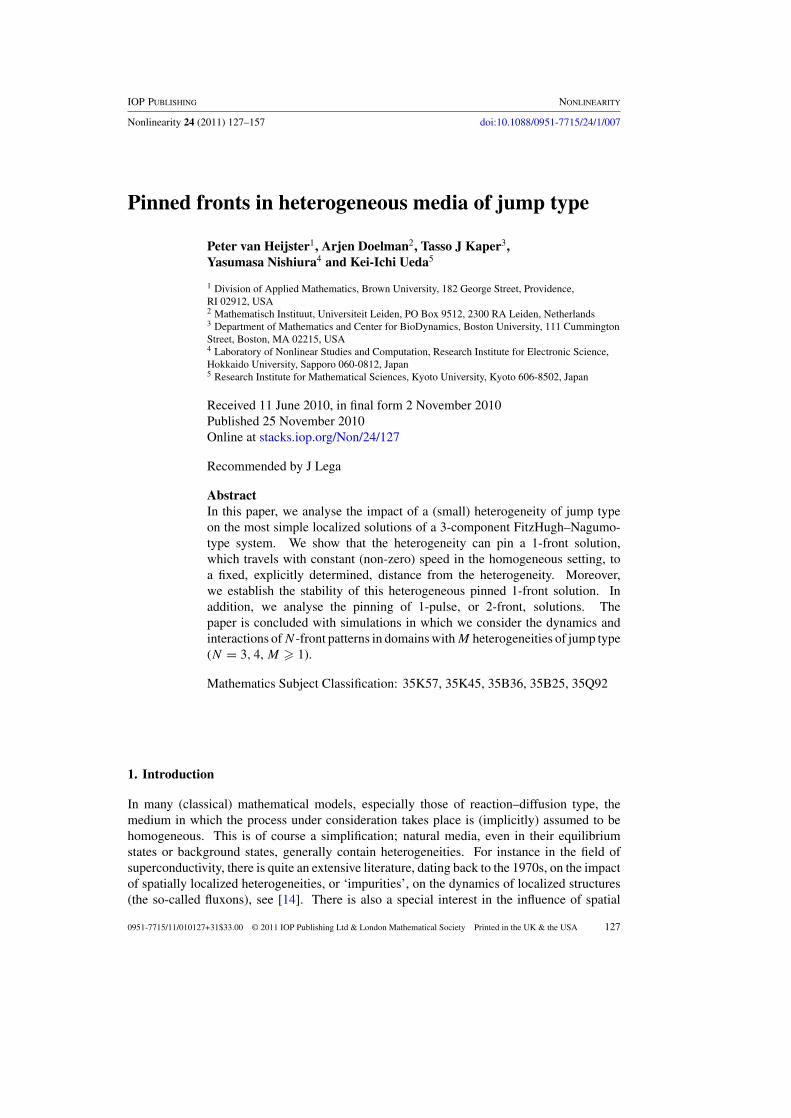
Figure 4. In this figure, we look at the influence of the heterogeneity on the dynamics of 2-frontsolutions. The system parameters (α, β, D, τ, θ, ε) are fixed at (3, 2, 5, 1, 1, 0.01) and the stepfunction is γ1 = 2 and γ2 = −1 (case (b)). The initial positions of the front and back are differentin the left and two right frames. In the left frame, the initial position of the back is taken to theright of the heterogeneity and we observe that this back travels to infinity, while the front evolvesto a stationary pinned 1-front solution at the heterogeneity. In the middle frame, the initial positionof the back is taken to the left of the heterogeneity and the structure evolves to a stationary 2-frontsolution pinned away from the heterogeneity. The right frame shows the final structure of this lastsimulation. The width of the 2-front is ξ2f = 160 and the distance to the heterogeneity is ξ∗ = 160.

Note that the thick black dashed line again indicates the position of the heterogeneity.

From theorem 1.3 we know that for these system parameters the homogeneous problempossesses a stationary stable 2-front solution for 0 < γ < 5 since α = 3, β = 2.Representative cases are γ1 = ±2 and γ2 = ±1. Moreover, from theorem 1.2 we see forthe homogeneous case the competition between on the one hand α and β and on the otherhand γ . When these parameters are all positive, the α and β components increase the distancebetween a front and a back (labelled with �), while the γ component decreases this distance.We will also see this competition in some of the simulations of cases (b) and (c).

We start with case (a) γ1 = −2 and γ2 = −1. Since both γi’s are negative, the equivalenthomogeneous problems possess no stationary stable 2-front solutions, see theorem 1.3. Afront and a back repel each other as can be explained from theorem 1.2. For the heterogeneousproblem we observe the same. The front and back travel in opposite directions towards infinityindependent of the initial positions of the front and back. Note that this behaviour is not shown.

Next, we analyse case (b) γ1 = 2 and γ2 = −1. For this step function there exists a stablepinned 1-front solution (and an unstable pinned 1-back solution), see theorems 2.1 and 3.1.This is exactly what we observe numerically, if we take the initial position of the back to theright of the heterogeneity (ξ > 0), the front gets pinned at the heterogeneity, while the backtravels to infinity, see the left frame of figure 4. However, since to the left of the heterogeneity(ξ < 0), γ (ξ) > 0, we expect that we can find pinned 2-front solutions in this region, seetheorem 1.3. This is also observed numerically, if we take the initial position of the back to theleft of the heterogeneity (ξ < 0), we obtain a pinned solution which is pinned away from andto the left of the heterogeneity. The width of the pinned 2-front solution is ξ2f = 160, whichagrees (to leading order in O(ε−1)) with the predicted homogeneous widths ξ

γ

hom (1.5). Moreprecisely, for γ = 2 the predicted homogeneous width is ξ 1

hom = 167. Note that the observeddistance of the 2-front solution to the heterogeneity is ξ ∗ = 160. See the right two frames offigure 4.

For the last case (c) γ1 = 2 and γ2 = 1, the equivalent homogeneous problems have forboth γi a stable stationary 2-front solution, see theorem 1.3. So, a priori, we could expect tofind stationary solutions in both regimes. If we take the initial position of the back to the right of


0

1

2

3

4

10!

6-600

-400

-200

0

200

400

600

-1

0

1

0

1

2

3

4-600

-400

-200

0

200

400

600

-1

0

1

-500 -400 -300 -200 -100 0 100 200 300 400 500

-1

-0.8

-0.6

-0.4

-0.2

0

0.2

0.4

0.6

0.8

1

5

x 10!

4

-500 -400 -300 -200 -100 0 100 200 300 400 500

-1

-0.8

-0.6

-0.4

-0.2

0

0.2

0.4

0.6

0.8

1

Figure 5. In this figure, we look at the influence of the heterogeneity on the dynamics of 2-frontsolutions. The system parameters (α, β, D, τ, θ, ε) are fixed at (3, 2, 5, 1, 1, 0.01) and the stepfunction is γ1 = 2 and γ2 = 1 (case (c)). The initial positions of the front and back vary inthe frames. In the left two frames, the initial position of the back is taken to the right of theheterogeneity and we observe that the structure evolves to a stationary pinned 2-front solution atthe heterogeneity. The width of the 2-front solution is ξ2f = 340 (the second frame shows the finalstructure of the simulation). In the right two frames, the initial position of the back is taken to theleft of the heterogeneity and the structure evolves to a stationary 2-front solution pinned away fromthe heterogeneity . The width of the 2-front is ξ2f = 160 and the distance to the heterogeneity isξ∗ = 115. Note that the thick black dashed line again indicates the position of the heterogeneity.

the heterogeneity (ξ > 0), the solution asymptotes to a stationary 2-front solution whose frontis located at the heterogeneity. The width of the pinned 2-front solution is ξ2f = 340, whichagrees (to leading order in O(ε−1)) with the predicted homogeneous widths ξ

γ

hom (1.5). Moreprecisely, for γ = 1 the predicted homogeneous width is ξ 1

hom = 381. See the left two framesof figure 5. However, if we take the initial position of the back to the left of the heterogeneity(ξ < 0), we again obtain a pinned solution, but now the solution is pinned away from and to theleft of the heterogeneity. The width of the pinned 2-front solution is ξ2f = 160, which agrees(to leading order in O(ε−1)) with the predicted homogeneous widths ξ

γ

hom (1.5). Moreover,the distance of the 2-front solution to the heterogeneity is ξ ∗ = 115. See the right two framesof figure 5. These simulations suggest the existence of an unstable scatter solution [18, 25],see also remark 1.2. Moreover, they suggest, as is also observed in the numerical simulationsin [18, 25], that pinned solutions prefer smaller γ . That is, we do not find any pinned solutionswhose back is located at the heterogeneity (γ (ξ) = γ1 = 2), but we do find pinned solutionswhose front is located at the heterogeneity (γ (ξ) = γ2 = 1). Note that this actually followsfrom the existence condition γ1 > γ2 of theorem 1.5 or 4.1. Finally, note that the distance tothe heterogeneity ξ ∗ for cases (b) and (c) differs. This suggests that also for this type of pinnedsolutions (see remark 1.2) the step function influences the distance to the heterogeneity ξ ∗.

4.2. Existence analysis

In this section, we determine the existence condition for pinned 2-front solutions whose frontsare located near the heterogeneity and which asymptotes to (U, V, W) = u−

γ1(1, 1, 1) (1.6).

The ideas behind the analysis are similar to those of section 2 and of [5]. However, since wewill find that ξ ∗ � 1 but still inside If , i.e. the distance between the front and the heterogeneitywill be � 1 and � ε−1/2 (see (4.1)), we have to perform a higher order analysis. Nevertheless,we will not go into all the details of the proof, see remark 2.1.

Theorem 4.1. For each D > 1, τ, θ > 0, α, β ∈ R, γ1,2 ∈ R\{0}, and for each ε > 0small enough, there exists a pinned 2-front solution �2f(ξ) which asymptotes to (U, V, W) =u−

γ1(1, 1, 1) (1.6) as ξ → −∞ and whose front is located near the heterogeneity, if and only if


γ1 > γ2 and there exists a ξ2f solving


ξ2f = γ2. (4.1)

Moreover, the width of the 2-front solution is ξ2f and the distance of the heterogeneity to thefront ξ ∗ is given by

ξ ∗ = − 12

√2 log

(18ε(γ1 − γ2)

). (4.2)

Note that the existence condition indeed coincides with the existence condition (1.5) forthe homogeneous problem with γ = γ2. Moreover, from the system symmetry (1.9) we obtainthat a pinned solution with its back near the heterogeneity will form if γ2 > γ1 (and an existencecondition like (4.1) with γ2 replaced by γ1). This coincides with the numerical observationthat stationary 2-front solutions prefer smaller (positive) γ . See also the left frame of figure 5.

Unlike for the 1-front solutions, we refrain from explicitly studying the stability of thepinned 2-front solutions. There are two reasons for this: (i) one does not have to develop newideas to perform this stability analysis; (ii) since we have to consider higher order effects inthe existence analysis, we also need to go (at least) one order higher in the stability analysis,and this requires quite a calculational effort.

Proof of theorem 4.1. The proof will be a combination of the proof of the heterogeneous1-front solution (see section 2) and the proof of the homogeneous 1-front solution [5]. Thefront ‘sees’ the heterogeneity, while the back ‘does not see’ the heterogeneity. We first define ξ ∗

as the ξ value for which the U component crosses zero for the first time, that is, U(ξ ∗) = 0, andU ′(ξ ∗) > 0. Moreover, define ξ 2 as the second zero of the U component, that is, U(ξ 2) = 0,

andU ′(ξ 2) < 0. By assumption, ξ ∗ < ξ 2, and the width of the 2-front is given by ξ2f := ξ 2−ξ ∗.We introduce three slow fields and two fast fields:

I 1s :=

(−∞, − 1√

ε+ ξ ∗

), I 2

f :=[− 1√

ε+ ξ ∗,

1√ε

+ ξ ∗]

,

I 3s :=

(1√ε

+ ξ ∗, − 1√ε

+ ξ 2

), I 4

f :=[− 1√

ε+ ξ 2,

1√ε

+ ξ 2

], I 5

s :=(

1√ε

+ ξ 2, ∞)

,

with 0 ∈ I 2f . Next, we reduce the heterogeneous PDE (1.2) to the same six-dimensional system

of first order ODEs (2.2) as in section 2, and we split it into two different systems of ODEs(2.2)1 and (2.2)2 as before. We are interested in solutions 2f(ξ) which still asymptote to P −

(2.3) as ξ → −∞. However, we have a different asymptotic state at plus infinity:

(u, p, v, q, w, r) = (u−γ2

, 0, u−γ2

, 0, u−γ2

, 0) := P −2f ,

see (1.6). We now have that

2f(ξ) ⊂ Wu(P −) ∩ Ws(P −2f ) ,

and again the solutions of (2.2)1 and (2.2)2 should match up at zero.Also the FRS is the same, and thus has the same Hamiltonian structure and the same

homoclinic solutions, see (2.6)–(2.8). But now also (u+(ξ), p+(ξ)) is relevant, since in thesecond fast field I 4

f (u(ξ), p(ξ)) is asymptotically close to (u+(ξ − ξ 2), p+(ξ − ξ 2)) [5].We now need to distinguish between four, instead of two ((2.9) and (2.10)), persisting slowmanifolds:

M−i := {

(u, p, v, q, w, r) | u = −1 − 12ε(αv + βw + γi) + O(ε2), p = O(ε2)

},

M+i := {

(u, p, v, q, w, r) | u = 1 − 12ε(αv + βw + γi) + O(ε2), p = O(ε2)

}, i = 1, 2.

(4.3)


In the slow field I 1s , the flow of (2.2) is exponentially close to M−

1 . In I 3s , the flow is

exponentially close to M+2 and in I 5

s , it is exponentially close to M−2 . Moreover, the flow

on the slow manifolds M−1,2 is to leading order given by (2.11), while the leading order flow

on M+1,2 is given by (2.12), see [5].

Next, we employ the Melnikov-type approach. In the first fast field I 2f , the approach

will be the same as that used in section 2, since the heterogeneity lies in this fast field. Bycontrast, in the second fast field I 4

f , the approach will be similar to that used in [5], since theheterogeneity does not lie in this fast field. Moreover, the slow v, w components are, to leadingorder, still constant during the jumps over both fast fields, see (2.13) and [5]. This results inthe eight constants,

(v, q, w, r) = (v20, q

20 , w2

0, r20 ) in I 2

f , (v, q, w, r) = (v40, q

40 , w4

0, r40 ) in I 4

f . (4.4)

The values of Hamiltonian (2.7) on the four slow manifolds M±1,2 are given by (2.14), and we

determine the change in the Hamiltonian over the fast fields two times in two different ways.We start with the fast field I 2

f containing the heterogeneity. Since H(2(ξ)) → H |M−1

forξ ↓ I 1

s and H(2(ξ)) → H |M+2

for ξ ↑ I 3s , we obtain that during the jump through this fast

field, the Hamiltonian changes in an O(ε2) fashion,

�2f H = H |M+

2− H |M−

1= 1

4ε2(γ1 − γ2)(2αv20 + 2βw2

0 + γ2 + γ1) + O(ε2√ε), (4.5)

see (2.15) and (4.3). On the other hand, since the fast component of 2f(ξ) in I 2f is to leading

order given by (u−(ξ − ξ ∗), p−(ξ − ξ ∗)) (see (2.8)), we also obtain

�2f H =

∫I 2f

Hξ dξ (4.6)

= 2ε(αv20 + βw2

0) + εγ1

(1 − tanh

(12

√2ξ ∗

))+ εγ2

(1 + tanh

(12

√2ξ ∗

))+ O(ε

√ε),

see (2.16). This yields the first jump condition. To leading order, we have that

0 = 2(αv20 + βw2

0) + γ1

(1 − tanh

(12

√2ξ ∗

))+ γ2

(1 + tanh

(12

√2ξ ∗

)). (4.7)

Next, we analyse the second jump, the jump through the fast field I 4f . Since H(2(ξ)) →

H |M+2

for ξ ↓ I 3s and H(2(ξ)) → H |M−

2for ξ ↑ I 5

s , we find that

�4f H = H |M−

2− H |M+

2= O(ε2√ε) .

On the other hand, since the fast component of 2f(ξ) in I 4f is to leading order given by

(u+(ξ − ξ 2), p+(ξ − ξ 2)) (see (2.8)), we get

�4f H =

∫I 4f

Hξ dξ = −2ε(αv40 + βw4

0 + γ2) + O(ε√

ε).

This yields the second jump condition. To leading order, we obtain

0 = αv40 + βw4

0 + γ2. (4.8)

Note that both jump conditions (4.7) and (4.8) depend on ξ ∗ and ξ 2 through the slow constants(v

2,40 , w

2,40 ) (4.4). To determine these slow constants, we return to the slow equations (2.11)

and (2.12) in the slow fields. After integrating the equations, implementing the asymptotic


behaviour and matching the solutions over the fast fields, we obtain

v(ξ) =

eε(ξ−ξ∗) − eε(ξ−ξ 2) − 1, ξ ∈ I 1

s ,

−eε(ξ−ξ 2) − e−ε(ξ−ξ∗) + 1, ξ ∈ I 3s ,

e−ε(ξ−ξ 2) − e−ε(ξ−ξ∗) − 1, ξ ∈ I 5s ,

(4.9)

and

w(ξ) =

eεD

(ξ−ξ∗) − eεD

(ξ−ξ 2) − 1, ξ ∈ I 1

s ,

−eεD

(ξ−ξ 2) − e− εD

(ξ−ξ∗) + 1, ξ ∈ I 3s ,

e− εD

(ξ−ξ 2) − e− εD

(ξ−ξ∗) − 1, ξ ∈ I 5s .

(4.10)

Therefore, v20 = v0(ξ

∗) = v40 = v(ξ 2) = −e−ε(ξ 2−ξ∗) and w2

0 = w40 = −e− ε

D(ξ 2−ξ∗).

First, we plug the values of these constants into the second jump condition (4.8) and recallthat ξ2f = ξ 2 − ξ ∗, to obtain the existence condition determining the width of the 2-frontsolution,


ξ2f = γ2,

see (4.1). Since v20 = v4

0 and w20 = w4

0, the first jump condition (4.7) reduces to leadingorder to

0 = − 2γ2 + γ1

(1 − tanh

(12

√2ξ ∗

))+ γ2

(1 + tanh

(12

√2ξ ∗

))�⇒

0 = (γ1 − γ2)(

1 − tanh(

12

√2ξ ∗

)).

Since γ1 �= γ2, this equation is fulfilled only if tanh ( 12

√2ξ ∗) = 1 to leading order. This

implies that ξ ∗ � 1. Note that this does not necessarily imply that 0 /∈ I 2f . To find out, we

need to look at the next order in the fast field I 2f to determine ξ ∗.

First, we introduce a regular expansion of the fast u component in the fast field I 2f :

u(ξ) = tanh

(1

2

√2(ξ − ξ ∗)

)+

εu2,11 + O(ε2), ξ ∈

[− 1√

ε+ ξ ∗, 0

),

εu2,21 + O(ε2), ξ ∈

[0,

1√ε

+ ξ ∗]

.

(4.11)

However, it will not be necessary to determine u2,11 and u

2,21 explicitly. By (4.8) and since

v20 = v4

0 and w20 = w4

0, (4.5) reduces to

�2f H = 1

4ε2(γ1 − γ2)2 + O(ε2√ε).

We obtain the higher order jump condition, by equating this with (4.6),

ε

∫I 2f

p(ξ)(αv(ξ) + βw(ξ) + γ (ξ)) dξ = 14ε(γ1 − γ2)

2 + O(ε√

ε). (4.12)

Recall from (2.13) that in the fast field I 2f

v(ξ) = v20 + εq2

0 (ξ − ξ ∗) + O(ε2), w(ξ) = w20 +

ε

Dr2

0 (ξ − ξ ∗) + O(ε2),

with q20 = 1 + v2

0 and r20 = 1 + w2

0, see (4.9) and (4.10).


Therefore, the integral of (4.12) can be written as∫I 2f

p(ξ)(αv(ξ) + βw(ξ) + γ (ξ)) dξ = (αv20 + βw2

0 + γ1)

∫ 0

−∞

(tanh

(1

2

√2(ξ − ξ ∗)

))ξ

dξ

+ (αv20 + βw2

0 + γ2)

∫ ∞

0

(tanh

(1

2

√2(ξ − ξ ∗)

))ξ

dξ

+ ε

(α

(1 + v2

0

)+

β

D(1 + w0)

)

×∫

I 2f

(ξ − ξ ∗)(

tanh

(1

2

√2(ξ − ξ ∗)

))ξ

dξ

+ ε(αv20 + βw2

0 + γ1)

∫ 0

−∞(u

2,11 )ξ dξ

+ ε(αv20 + βw2

0 + γ2)

∫ ∞

0(u

2,21 )ξ dξ + O(ε

√ε)

= (γ1 − γ2)

∫ 0

−∞

(tanh

(1

2

√2(ξ − ξ ∗)

))ξ

dξ

+ ε

(α

(1 + v2

0

)+

β

D(1 + w0)

)

×∫

I 2f

(ξ − ξ ∗)(

tanh

(1

2

√2(ξ − ξ ∗)

))ξ

dξ

+ ε(γ1 − γ2)

∫ 0

−∞(u

2,11 )ξ dξ + O(ε

√ε).

However, the second and third integrals are zero to leading order. The second integral is zerosince the integrand is an odd function around the centre of I 2

f . The third integral vanishes

to leading order since ξ ∗ � 1 and therefore u2,11 (−∞) = u

2,11 (0), see (4.11). So, the only

remaining integral must be equal to the right-hand side of (4.12). To leading order, we obtain

1

4ε(γ1 − γ2) =

∫ 0

−∞

(tanh

(1

2

√2(ξ − ξ ∗)

))ξ

dξ

= tanh

(1

2

√2(ξ − ξ ∗)

)∣∣∣∣0

−∞

= − tanh

(1

2

√2ξ ∗

)+ 1 + O(ε2)

= 2e−√2ξ∗

1 + e−√2ξ∗ + O(ε2).

Therefore, to leading order

ξ ∗ = − 12

√2 log

(18ε(γ1 − γ2)

),

see (4.2). Note that this ξ ∗ is only defined if γ1 > γ2 and also note that 0 ∈ I 2f . This completes

the proof, see remark 2.1. �

Lemma 4.2. For the heterogeneous problem, there does not exist a pinned 2-front solution forwhich the heterogeneity in γ (ξ) lies in between the front and the back, that is, 0 ∈ I 3

s .


Proof. An analysis similar to the previous proof gives the following two jump conditions, see(4.7) and (4.8):


ξ2f = γ1,


ξ2f = γ2,(4.13)

where, as before, ξ2f is the width of the 2-front solution . Since γ1 �= γ2, we obtain that (4.13)has no solutions. �

5. Numerical simulations

In this section, we show numerical results for several more complex localized structures such as3-front solutions, 4-front solutions and travelling 2-front solutions. We also show the dynamicsof 2-front solutions for different types of heterogeneities, more precisely, for bump, or 2-jump,heterogeneities and periodic heterogeneities. Also, where possible, we qualitatively explainthe observed dynamics for these complex cases from the 1-front and 2-front dynamics withstep function heterogeneity derived in the previous sections.

It should be noted that the approach developed here can, in combination with themethods of [5, 22, 21], in principle be used to analytically study many of the forthcominginteractions between N -front patterns and M-jump heterogeneities. However, the calculationalcomplications will rapidly become overwhelming. Nevertheless, our methods, in principle,enable us to—for instance—explicitly study the pinning of a 3-front solution by a 1-jumpheterogeneity (see figure 6(c)), or that of a 2-front by a 2-jump heterogeneity (see figure 8(b)).However, it should be remarked that several of the simulations to be presented in this sectionexhibit a pinning of fronts that takes place in a slow field. This situation has not yet been studied,see remark 1.2. After this type of ‘weak interactions’ has been understood for stationarypatterns, one can—again in principle—take the next step and deduce explicit evolutionequations for the interactions between fronts and heterogeneities as was done in [22] forthe homogeneous problem. Finally, it should be explicitly remarked that the case τ = O(ε−2)

is still largely not understood, even in the homogeneous case, see [5, 21, 22] and figure 10.In our simulations, we focus on the influence of the heterogeneity. Therefore, we keep most

of the other system parameters fixed in this section, i.e. (α, β, D, τ, θ, ε) = (3, 2, 5, 1, 1, 0.01),except in section 5.5, where we also increase τ to 8600. When we use the step functionheterogeneity (1.3), we can, by the system symmetry (1.9), restrict ourselves to a fewcombinations for γ1 and γ2. Moreover, since the homogeneous problem possesses no stationarysolutions if |γ | > |α+β| (see theorem 1.3), we only need to look at a few different cases of signcombinations and magnitudes of γ1 and γ2. Representative cases are given by γ1 = ±1 andγ2 = ±2. Typically, the observed dynamics seems to be generic, that is, for slightly differentparameter values the dynamics is not drastically different.

5.1. Dynamics of 3-front solutions

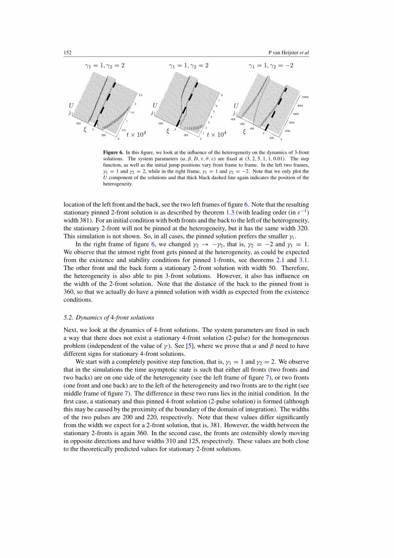
We start by analysing the influence of the step function heterogeneity (1.3) on the dynamics of3-front solutions. First, we take a completely positive step function: γ1 = 1, γ2 = 2. For thehomogeneous problem (with γ (ξ) = γ1 or γ (ξ) = γ2), the utmost right front travels to plusinfinity, and the remaining front and the back form a stationary 2-front [22]. This is also whatwe observe for the heterogeneous case. However, the location of the resulting stationary pinned2-front solution depends on the initial positions of the fronts and back. If the initial positionof the right front is to the right of the heterogeneity, the stationary 2-front will be pinned withits back to the heterogeneity, and it has an approximate width of 320, irrespective of the initial


0

1

2

3

4

5

6

7

8

-500

0

500

-101

t

0

0.5

1

1.5

2

2.5

-500

0

500

-101

t

U

0

2000

4000

6000

8000

10000

-600

-400

-200

0

200

-101

Figure 6. In this figure, we look at the influence of the heterogeneity on the dynamics of 3-frontsolutions. The system parameters (α, β, D, τ, θ, ε) are fixed at (3, 2, 5, 1, 1, 0.01). The stepfunction, as well as the initial jump positions vary from frame to frame. In the left two frames,γ1 = 1 and γ2 = 2, while in the right frame, γ1 = 1 and γ2 = −2. Note that we only plot theU component of the solutions and that thick black dashed line again indicates the position of theheterogeneity.

location of the left front and the back, see the two left frames of figure 6. Note that the resultingstationary pinned 2-front solution is as described by theorem 1.3 (with leading order (in ε−1)width 381). For an initial condition with both fronts and the back to the left of the heterogeneity,the stationary 2-front will not be pinned at the heterogeneity, but it has the same width 320.This simulation is not shown. So, in all cases, the pinned solution prefers the smaller γi .

In the right frame of figure 6, we changed γ2 → −γ2, that is, γ2 = −2 and γ1 = 1.We observe that the utmost right front gets pinned at the heterogeneity, as could be expectedfrom the existence and stability conditions for pinned 1-fronts, see theorems 2.1 and 3.1.The other front and the back form a stationary 2-front solution with width 50. Therefore,the heterogeneity is also able to pin 3-front solutions. However, it also has influence onthe width of the 2-front solution. Note that the distance of the back to the pinned front is360, so that we actually do have a pinned solution with width as expected from the existenceconditions.

5.2. Dynamics of 4-front solutions

Next, we look at the dynamics of 4-front solutions. The system parameters are fixed in sucha way that there does not exist a stationary 4-front solution (2-pulse) for the homogeneousproblem (independent of the value of γ ). See [5], where we prove that α and β need to havedifferent signs for stationary 4-front solutions.

We start with a completely positive step function, that is, γ1 = 1 and γ2 = 2. We observethat in the simulations the time asymptotic state is such that either all fronts (two fronts andtwo backs) are on one side of the heterogeneity (see the left frame of figure 7), or two fronts(one front and one back) are to the left of the heterogeneity and two fronts are to the right (seemiddle frame of figure 7). The difference in these two runs lies in the initial condition. In thefirst case, a stationary and thus pinned 4-front solution (2-pulse solution) is formed (althoughthis may be caused by the proximity of the boundary of the domain of integration). The widthsof the two pulses are 200 and 220, respectively. Note that these values differ significantlyfrom the width we expect for a 2-front solution, that is, 381. However, the width between thestationary 2-fronts is again 360. In the second case, the fronts are ostensibly slowly movingin opposite directions and have widths 310 and 125, respectively. These values are both closeto the theoretically predicted values for stationary 2-front solutions.


0

0.5

1

1.5

2

2.5

-1000

-500

0

500

1000

-101

0

0.5

1

1.5

2

2.5

3

-600

-400

-200

0

200

400

600

800

-101

0

1

2

3

4

5

6

7

8

-800

-600

-400

-200

0

200

400

600

800

-101

Figure 7. In this figure, we look at the influence of the heterogeneity on the dynamics of the4-front solution. The system parameters (α, β, D, τ, θ, ε) are fixed at (3, 2, 5, 1, 1, 0.01). Thestep function and the initial jump positions vary from frame to frame. In the left two frames,γ1 = 1 and γ2 = 2. In the right frame, γ1 = −1 and γ2 = 2. Note that we only plot the U

component of the solutions and that thick black dashed line again indicates the position of theheterogeneity.

In the right frame of figure 7, we took γ1 = −1 and γ2 = 2. The left most front travels(as expected) towards minus infinity, and the left most back gets pinned at the heterogeneity.The remaining front and back form a stationary 2-front with width 92, as was also observedfor the 3-front case, see the right frame of figure 6.

For a completely negative step function: γ1 = −1 and γ2 = −2, we observe that theouter front and back diverge, while the inner front and back form a stationary 2-front solution(mirrored to the ones constructed in the previous section). This stationary solution can belocated at the heterogeneity or away from the heterogeneity. Note that this simulation is notshown in figure 7.

5.3. A bump, or 2-jump, heterogeneity

In this section, we modify the heterogeneity from one step function to two step functions,which results in a so-called bump, or 2-jump, heterogeneity. We look at the influence on the2-front dynamics, see also [18]. More specifically,

γ (ξ) ={γ1, for ξ /∈ [A, B],γ2, for ξ ∈ [A, B].

(5.1)

We focus on the case where sgn(γ1) �= sgn(γ2), since for this combination fronts are expectedto be pinned, see theorems 2.1 and 3.1. More specifically, we set γ1 = ±1 and γ2 = ∓2.Moreover, we take −A = B = 150, such that stationary 2-front solutions can easily fit in thebump region (for γ (ξ) = γ2 = ±2).

First, we set γ1 = −1 and γ2 = 2 and take the initial positions of the front and back inthe bump region. The front and back evolve to a stationary 2-front solution with width 150(theoretically 167) and away from the heterogeneities, see the left frame of figure 8. So, itappears that the front and back do not actually see the heterogeneities. This could be expected,since from theorems 2.1 and 3.1, we expect that both heterogeneities push the nearby front orback away. If only one of the initial fronts is in between the heterogeneities, it moves to oneof the heterogeneities, while the other front or back moves towards plus/minus infinity. Thisrun is not shown in figure 8.

For γ1 = 1 and γ2 = −2, the dynamics of the 2-front is, as expected, completelyopposite. Now, the heterogeneities attract their nearby structure. If the initial jump positions


0

0.5

1

1.5

2

-200

-100

0

100

200

-101

0

500

1000

1500

2000

2500

-200

-100

0

100

200

-101

Figure 8. In this figure, we look at the bump heterogeneity (5.1) with −A = B = 150, indicatedby the dashed black lines. In the left frame, γ1 = −1, γ2 = 2, while in the right frame,γ2 = −2, γ1 = 1. The other system parameters are fixed at (α, β, D, τ, θ, ε) = (3, 2, 5, 1, 1, 0.01).Note that we only plot the U component of the solutions.

are chosen in between the heterogeneities, a stable stationary 2-front solution is formed at theheterogeneities. The front is located near the left heterogeneity A, while the back is located atthe right heterogeneity B, see the right frame of figure 8. If only one of the initial fronts is inbetween the heterogeneities, this front or back moves to one of the heterogeneities, however,in the opposite direction compared with the previous case (γ1 = −1 and γ2 = 2). The frontor back that lies outside the heterogeneities also becomes stationary. This latter simulation isnot shown in figure 8.

5.4. Periodic heterogeneities

In this section, we look at the dynamics of a 2-front solution in the presence of a periodicheterogeneity. First, we look at a periodic smoothened bump heterogeneity with period 200and which oscillates between 1 and −1, that is,

γ (ξ) = 1 +20∑i=1

(−1)i−1 tanh (10 (ξ − (950 − 100 ∗ (i − 1)))) . (5.2)

An initial condition for which the front and back are relatively close to each other evolves toa stationary solution. However, the front and the back do not evolve in a symmetric fashion.Moreover, while the back gets pinned at a heterogeneity, the front is pinned near a heterogeneity,see the left frame of figure 9. Compare also with the right frame of figure 8, where the samebehaviour is observed for the front (and the back).

Second, as in [18], we take a sinusoidal periodic heterogeneity. More specifically, theforcing parameter reads γ (ξ) = sin (0.1ξ) such that γ (ξ) ∈ [−1, 1] and the period of thefunction is 20π . The front and the back again move asymmetrically to a stationary solutionwith fixed width, see the middle frame of figure 9. In the right frame, we plot the U componentof the final stationary solution after 10 000 time steps together with (a part of) the periodicforcing parameter γ (ξ) (dotted line). We observe that for the stationary solution the value ofγ at the position of the front and back are the same and around 0.85. However, the width ofthe stationary solution does not coincide with the width of a stationary 2-front solution in thehomogeneous case with this particular value of γ .


-300 -200 -100 0 100 200 300

-1

-0.8

-0.6

-0.4

-0.2

0

0.2

0.4

0.6

0.8

1

0

1000

2000

3000

4000

5000

6000

7000

8000

9000

10000

-300

-200

-100

0

100

200

300

-101

0

1000

2000

3000

4000

5000

6000

-200

-100

0

100

200

-101

Figure 9. In the left frame, we plot the evolution of the U component of a 2-front solutionwith a periodic smoothened bump heterogeneity (5.2). The dotted lines are the zeros of γ (ξ).In the middle frame, we plot the dynamics of the U component of a 2-front solution with asinusoidal periodic heterogeneity γ (ξ) = sin (0.1ξ). The other system parameters are fixed(α, β, D, τ, θ, ε) = (3, 2, 5, 1, 1, 0.01). In the right frame, we plot this U component after the10 000 time steps. The dotted line represents the periodic forcing parameter γ (ξ).

5.5. Large τ

In this last section, we discuss maybe the most interesting case, τ = O(ε−2) large, see also [22].From the homogeneous analysis [5, 21], we know that in this case the stationary 2-front solutioncan bifurcate into a uniformly travelling 2-front solution or into a symmetrically breathing2-front solution.

We consider only one heterogeneity and we keep the system parameters (α, β, D, τ, θ, ε)

positive and fixed at (3, 2, 5, 8600, 1, 0.01). The most interesting dynamics is observed whenboth γi’s are positive, that is, γ1 = 1 and γ2 = 2, since in this case the homogeneous equivalentwould yield both travelling and breathing 2-front solutions. The observed behaviour for theheterogeneous case relies heavily on the initial conditions. However, we observe simultaneoustravelling and breathing behaviour, see the left two frames of figure 10. Note that to the right ofthe heterogeneity the solution seems to travel and breath, while to the left of the heterogeneityit only seems to travel. Moreover, we observe a travelling solution which sometimes bouncesof the heterogeneity and sometimes not, see the right frame of figure 10.

If only one of the γi’s is positive, one of the fronts gets pinned at the heterogeneity,while the other one travels to plus/minus infinity, as could be expected from the 1-frontanalysis. This behaviour is not shown. The homogeneous problem with negative γ possessesno uniformly travelling or breathing 2-front solutions [5]. For the heterogeneous problem,we obtain something similar: if both γi’s are negative, the front and back move in oppositedirections towards plus/minus infinity. This simulation is also not shown.

Acknowledgments

The authors thank P Zegeling for his valuable assistance with the software used in thenumerical simulations. PvH and AD gratefully acknowledges support from the NetherlandsOrganisation for Scientific Research (NWO) and the Centrum Wiskunde & Informatica(CWI). PvH also thanks YN and Hokkaido University for their hospitality. TK gratefullyacknowledges support from the National Science Foundation through grant DMS-0606343.YN gratefully acknowledges support from the Grant-in-Aid for Scientific Research underGrant No (B)16204008. KIU gratefully acknowledges support from the FY 2008 Researcher


Figure 10. In this figure, we plot the dynamics of a 2-front solution with step function heterogeneityand τ = 8600 large. The other system parameters are fixed during the simulation. That is,(α, β, D, θ, ε) = (3, 2, 5, 1, 0.01). Moreover, also the heterogeneity is kept fixed: γ1 = 1 andγ2 = 2. So, the only thing changing from frame to frame is the initial positions. Note that we onlyplot the U component of the solutions and that thick black dashed line again indicates the positionof the heterogeneity.

Exchange Program between JSPS and NWO. KIU also thanks AD, PvH and CWI for theirhospitality.

References

[1] Derks G, Doelman A, van Gils S A and Susanto H 2007 Stability analysis of π -kinks in a 0-π Josephson junctionSIAM J. Appl. Dyn. Syst. 6 99–141

[2] Dirr N and Yip N K 2006 Pinning and de-pinning phenomena in front propagation in heterogeneous mediaInterfaces Free Bound. 8 79–109

[3] Doelman A, Kaper T J and Promislow K 2007 Nonlinear asymptotic stability of the semistrong pulse dynamicsin a regularized Gierer–Meinhardt model SIAM J. Math. Anal. 38 1760–87

[4] Doelman A and van der Ploeg H 2002 Homoclinic stripe patterns SIAM J. Appl. Dyn. Syst. 1 65–104[5] Doelman A, van Heijster P and Kaper T J 2009 Pulse dynamics in a three-component system: existence analysis

J. Dyn. Diff. Eqns 21 73–115[6] Ei S I, Ikeda H and Kawana T 2008 Dynamics of front solutions in a specific reaction–diffusion system in one

dimension Japan J. Ind. Appl. Math. 25 117–47[7] Fenichel N 1971/1972 Persistence and smoothness of invariant manifolds for flows Indiana Univ. Math. J.

21 193–226[8] Henry D 1981 Geometric Theory of Semilinear Parabolic Equations (Lecture Notes in Mathematics vol 840)

(Berlin: Springer)[9] Ikeda H and Ei S-I 2010 Front dynamics in heterogeneous diffusive media Physica D 17 1637–49

[10] Ikeda H and Mimura M 1989 Wave-blocking phenomena in bistable reaction–diffusion systems SIAM J. Appl.Math. 49 515–38

[11] Ikeda H and Mimura M 1991 Stability analysis of stationary solutions of bistable reaction–variable diffusion-systems SIAM J. Math. Anal. 22 1651–78

[12] Jones C K R T 1995 Geometric singular perturbation theory Dynamical Systems (Montecatini Terme, 1994)(Lecture Notes in Mathematics vol 1609) (Berlin: Springer) pp 44–118

[13] Kaper T J 1999 An introduction to geometric methods and dynamical systems theory for singular perturbationproblems Analyzing Multiscale Phenomena using Singular Perturbation Methods (Baltimore, MD, 1998)(Proceedings of Symposia in Applied Mathematics vol 56) (Providence, RI: American Mathematical Society)pp 85–131

[14] McLaughlin D W and Scott A C 1978 Perturbation analysis of fluxon dynamics Phys. Rev. A 18 1652–80[15] Mielke A and Schneider G 1995 Attractors for modulation equations on unbounded domains—existence and

comparison Nonlinearity 8 743–68[16] Nishiura Y, Oyama Y and Ueda K-I 2007 Dynamics of traveling pulses in heterogeneous media of jump type

Hokkaido Math. J. 36 207–42

http://dx.doi.org/10.1137/060657984

http://dx.doi.org/10.4171/IFB/136

http://dx.doi.org/10.1137/050646883

http://dx.doi.org/10.1137/S1111111101392831

http://dx.doi.org/10.1007/s10884-008-9125-2

http://dx.doi.org/10.1007/BF03167516

http://dx.doi.org/10.1512/iumj.1972.21.21017

http://dx.doi.org/10.1016/j.physd.2010.04.008

http://dx.doi.org/10.1137/0149030

http://dx.doi.org/10.1137/0522103

http://dx.doi.org/10.1007/BFb0095239

http://dx.doi.org/10.1103/PhysRevA.18.1652

http://dx.doi.org/10.1088/0951-7715/8/5/006


[17] Nishiura Y, Teramoto T and Ueda K I 2003 Scattering and separators in dissipative systems Phys. Rev. E67 056210

[18] Nishiura Y, Teramoto T, Yuan X and Ueda K-I 2007 Dynamics of traveling pulses in heterogeneous media Chaos17 037104

[19] Or-Guil M, Bode M, Schenk C P and Purwins H-G 1998 Spot bifurcations in three-component reaction–diffusionsystems: the onset of propagation Phys. Rev. E 57 6432–37

[20] Schenk C P, Or-Guil M, Bode M and Purwins H-G 1997 Interacting pulses in three-component reaction–diffusionsystems on two-dimensional domains Phys. Rev. Lett. 78 3781–4

[21] van Heijster P, Doelman A and Kaper T J 2008 Pulse dynamics in a three-component system: stability andbifurcations Physica D 237 3335–68

[22] van Heijster P, Doelman A, Kaper T J and Promislow K 2010 Front interactions in a three-component systemSIAM J. Appl. Dyn. Syst. 9 292–332

[23] van Heijster P and Sandstede B 2010 Planar radial spots in a three-component FitzHugh–Nagumo systemsubmitted

[24] Xin J 2000 Front propagation in heterogeneous media SIAM Rev. 42 161–230[25] Yuan X, Teramoto T and Nishiura Y 2007 Heterogeneity-induced defect bifurcation and pulse dynamics for a

three-component reaction–diffusion system Phys. Rev. E 75 036220[26] Yuan X, Teramoto T and Nishiura Y 2010 Eigenvalue behaviors and bifurcation for spot dynamics in

heterogeneous media Commun. Pure Appl. Anal. accepted

http://dx.doi.org/10.1103/PhysRevE.67.056210

http://dx.doi.org/10.1063/1.2778553


http://dx.doi.org/10.1103/PhysRevLett.78.3781

http://dx.doi.org/10.1016/j.physd.2008.07.014

http://dx.doi.org/10.1137/080744785

http://dx.doi.org/10.1137/S0036144599364296


Documents

Pinned fronts in heterogeneous media of jump typemath.bu.edu/people/heijster/PAPERS/HETEROGENEOUS.pdf · Pinned fronts in heterogeneous media of jump type 129 0 ... three are needed