NBER WORKING PAPER SERIES

A MONETARY EQUILIBRIUM MODELWITH TRANSACTIONS COSTS

Julio J. Rotemberg

Working Paper No. 918

NATIONAL BUREAU OF ECONOMIC RESEARCH1050 Massachusetts Avenue

Cambridge MA 02138

September 1982

I wish to thank Bob Pindyck for helpful discussions. The researchreported here is part of the NBER's research program in EconomicFluctuations. Any opinions expressed are those of the author andnot those of the National Bureau of Economic Research.

NBER Working Paper #978September 1982

A Monetary Equilibrium Model with Transactions Costs

ABSTRACT

This paper presents the competitive equilibrium of an economy in

which people hold money for transactions purposes. It studies both the

steady states which result from different rates of monetary expansion

and the effects of such non—steady state events as an open market operation.

Even though the model features no uncertainty and perfect foresight, open

market operations affect aggregate output. In particular, a simultaneous

increase in money and governmental holdings of capital temporarily raises

aggregate capital and output while it lowers the real rate of interest

on capital.

Julio J. RotembergAlfred P. Sloan School of ManagementMassachusetts Institute of Technology50 Memorial Drive, E52—250Cambridge, MA 02139

(617) 253—2956

I. INTRODUCTION

The objective of this paper is to study the competitive equilibrium of

an economy in which people hold money for transactions purposes. As in the

models of Baumol (1952), Tobin (1956), Stockman (1981), Townsend (1982) and

Jovanovic (1982), but in contrast to those of Grandmont and Vounes (1973),

Lucas (1980) and Helpman (1982), households are also allowed to hold interest

bearing capital in addition to barren money. The main advantage of the

present model is that it is able to shed light on the effects of sud

nonsteady state events as open market operations.

Households pick the path of consumption optimally from their point of

view. Because it is costly to carry out financial transactions, people visit

their financial intermediary only occasionally. However, I do not let house-

holds pick optimally the length of the period during which they do not visit

their bank. For tractability, the assumption is made that households have a

constant interval during which they carry out no financial transactions.

A crucial feature of this paper is that, as in all free market econ-

omies, different households visit their banks at different times. This leads

to conclusions which are strikingly "Keynesian". Government interventions,

and in particular open market operations, have the ability to affect aggregate

output and the real rate of interest. This is true even though the model

features no uncertainty, full information, perfect foresight and perfectly

competitive markets for goods and money. Moreover, the effects of monetary

policies closely resemble those found in standard textbooks. In particular, a

one period monetary expansion leads to a higher level of output which persists

for some time. It also concurrently leads to low real interest rates.

The paper proceeds as follows: Section II presents the model. It shows

the maximization problems of the households and the firms, as well as the

—2—

institutional environment. Section III presents the perfect foresight equilib—

rium of the economy. It is a difference equation which exhibits saddle path

stability near that steady state which has positive consumption. Section IV

studies steady state inflation and welfare. It establishes that the level of

output is independent of the rate of inflation but that inflation affects

welfare negatively by distorting the intertemporal consumption decisions.

Section V is the heart of the paper since it discusses monetary policy outside

the steady state. Finally, Section VI presents some conclusions.

II THE MODEL

There is only one good which can both be consumed and invested. Total

output produced by firms in period t (Q) depends, via a constant returns to

scale production function, on the amount of labor hired at t and on

the amount of the good which was produced but not consumed at t—l. Since an

amount of labor [ is assumed to be supplied inelastically:

Kt 1Q =

—

) (1)

E

where f is an increasing and concave function. Workers are assumed to be paid

their marginal product. Tnerefore, the total return, denominated in period t

goods, from foregoing the consumption of an additional good at t—l, is given

1by l+rtl, where:

Kt1l+rtl = f'( —

) (2)L

There are 2n households. At time t, the households are assumed to

maximize the utility function given by:

tt 1i (3)

—3—

where is the consumption of household i at time T, and p is a discount

factor. The households have access to two assets, money and claims on capi-

tal. Money is the only medium of exchange. Moreover, visits to the financial

intermediary for the purpose of converting claims on capital into money are

costly. Therefore, as in the inventory theoretical models of Baumol (1952)

and Tobin (1956), households engage in these visits only sporadically. In

this paper it will be assumed at the outset that households exchange capital

for money every two periods. The assumption that households do not change the

timing of their financial transactions in response to events, is made mainly

for tractability. Except in stationary environments, it is very difficult to

solve for the optimal timing of these visits, particularly when households

pick their consumption path optimally.

Without loss of' generality, suppose that household i engages in finan-

cial transactions in the "even" periods, t, t+2, t+4 At these dates it

withdraws an amount M' of' money balances which must be sufficient toT

pay for its consumption at 'r and T-1-1:

H' = p'+ c' (4)T TT T4-lTl

where P is the nominal price of the consumption and investment good at

T. The evolution of K1, the claims on capital of household i at 'r

is given by:

1

K+< B = (1 + rt 2< 2)(l +

1 1+(l÷r÷2k 1)Yt+z< 1 + 't+2k k 0,1,2,... (5)

Here, B is the real cost of visiting the financial intermediary, while Y is

the noninvestment income of' the household at 'r. This noninvestment income

—4—

includes labor income as well as taxes and transfers from the government.

Equation (5) says that investments minus brokerage fees at t+2< have to be

equal to total resources at ti-2k. These resources include the capitalized

values of' 2ad of noncapital income at t-4-2k—l, as well as current

noncapital income. Note that (5) explicitly assumes that noncapital income

is directly invested in claims on capital. This assumption considerably

simplifies the analysis.

The optimal path of consumption is found in two steps. First, I derive

consumption at T and Tl as a function of M. Then I derive the optimal values

of the sequence of monetary withdrawals.

The first step requires the maximization of:

lnC'+plnC' (6)T 't+l

subject to (4). This yields:2

pP . M1

c' — Tl - _..P__.I_. 7—P

—l+pP

T-I-l

Using (7), the expression in (6) is given by:

H'

lnC + plnC'1 = (l+p)ln( j1- ) + plflp — (l+p)ln(l+p)

P- pln( D ) (8)

Ft

Equation (8) asserts that the appropriately weighted sum of the instan-

taneous utilities at T and T+l increases with H1 / P but is negatively af-

fected by inflation between T and Tl.

Substituting (8) into (3) and using (5), one obtains:

Vt = 2k {ln[(l+rt 2)(l+rt+2kl)K÷Z<2 + (l+rt+<+i)Yt+2<i

-5-

+ t+2k - B - K2<] - plnp + (l+p)ln(1+p) - pln(t÷2k+l

(9)

t+2k

This expression must now be maximized with respect to the sequence of claims

on capital. This maximization yields:3

21 p (l+r )(l+r )-

Mt 2kt 2k+ = 0 (10)

Using (7), (10) becomes:

cit+2k+2 2= p (l+rt+2<)(l+rt<+l) (11)

t+2k

Note that both (11) and (7) state that the marginal rate of substitution times

a rate of return is equal to one. The important distinction between the two

is that in (7) the rate of return is the rate of' return on money, while in

(11) it is the rate of' return on capital. Stochastic versions of (11) have

been statistically rejected using aggregate U.S. data by Mankiw (1981) and

Hansen and Singleton (1982). Their rejections may be due in part to their

neglect of the fact that in the presence of the transactions motive for

holding money, the ratio of marginal utilities of consumption separated by

different time intervals is related to rates of' return of assets with dif-

ferent characteristics.

Financial intermediaries receive the household's income and invest it in

claims on capital. They are also allowed to issue a certain quantity of'

money. The intermediaries are compensated for their services with the bro-

kerage fees, B, of' (5). Their function can best be understood by following

their .transactions in detail.

Between periods T and Tl the financial intermediaries have as their

assets the household's claims on capital as well as M units of money.

—6—

These can be thought of' as deposits at the Federal Reserve Bank. Their

liabilities are the household's claims on capital and the amount of money, M,

that the households who came to the bank at T withdrew but did not spend at t.

In period T--l, the financial intermediaries issue whatever amount of money

the households who visit them in period i-i-i require. The households then

buy goods from the firms. me firms return the money they receive from the

households to the intermediaries in partial payment of' their compensation to

workers and their debt to the households. The rest of' their obligations to

the banks is then paid in the form of' claims on Tl capital. Since the

firms have constant returns to scale, their total obligations towards the

households are given by:

K K KEf()_fI()KG=YL+KPf1() (12)

C C T t TC

where K6 is the amount of capital owned by the government at T K is the

amount owned by the private sector which is equal to K — K6 and is labor

income at T. The sales of' firms at ¶41 are given by aggregate consumption at

't+l, C÷1. So the debt of' firms held by households at the end of' T+l must be

equal to:

KCf( 'i) -c -K6 (13)

't+l t+1

I also assume that half' the households (n) visit the intermediaries in

the even periods t,t÷2,t+4,..., and the other half carry out their financial

transactions in the odd periods. The fact that only a subset of the house-

holds visit financial intermediaries in any given day is one of the main

features of reality which this paper seeks to reflect. It also is a feature

of the steady states studied by Jovanovic (1982). It turns out that the

assumption that households stagger their financial transactions is crucial to

—7—

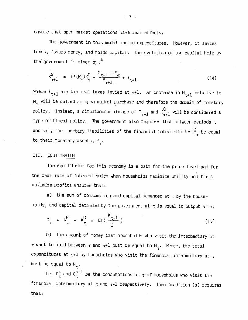
ensure that open market operations have real effects.

The government in this model has no expenditures. However, it levies

taxes, issues money, and holds capital. The evolution of the capital held by

thegovernment is given by:4

M -MK6 = f'(K )K6 + Tl T + T (14)TI-i T T P

where T1 are the real taxes levied at TI-l. An increase in MT+l relative to

MT will be called an open market purchase and therefore the domain of monetary

policy. Instead, a simultaneous change of and K641 will be considered a

type of fiscal policy. The government also requires that between periods T

and TI-]., the monetary liabilities of the financial intermediaries M be equal

to their monetary assets,MT.

III. EQUILIBRIUM

The equilibrium for this economy is a path for the price level and for

the real rate of interest which when households maximize utility and firms

maximize profits ensures that:

a) the sum of consumption and capital demanded at ' by the house-

holds, and capital demanded by the government at -r is equal to output at T.

KC + K .. K6 = Ef(i-) (15)T T T

b) The amount of money that households who visit the intermediary at

-r want to hold between T and TI-i must be equal to M. Hence, the total

expenditures at TI-i by households who visit the financial intermediary at-r

must be equal to M

Let C and CT be the consumptions at T of households who visit the

fThancial intermediary at - and -r—l respectively. Then condition (b) requires

that:

—8—

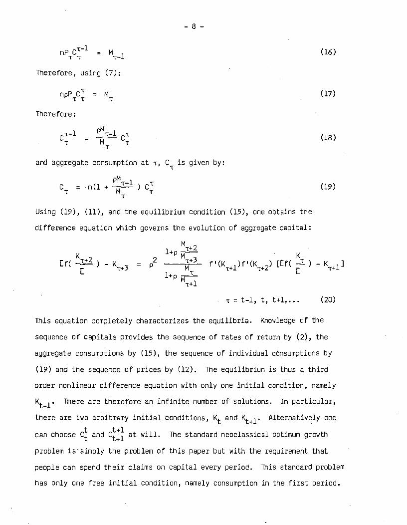
np c1 (16)TT T—l

Therefore, using (7):

flpP CT = M (17)TT T

Therefore:

pMCT_i = T-1

CT (18)T M T

T

and aggregate consumption at -r, CT is given by:

pM 1C n(i+__.i)cT (19)T M T

T

Using (19), (11), and the equilibrium condition (15), one obtains the

difference equation which governs the evolution of aggregate capital:

Mt+2

K lPj K

Ef( -'1-- ) - K÷3 = p2 -— f'(K1)f'(K2) [f( _i) - K÷1]C 1+Tl

-r = t—l, t, t+l,... (20)

This equation completely characterizes the equilibria. Knowledge of the

sequence of capitals provides the sequence of rates of return by (2), the

aggregate consurnptions by (15), the sequence of' individual cOnsumptions by

(19) and the sequence of prices by (12). The equilibrium is thus a third

order nonlinear difference equation with only one initial condition, namely

Kti. There are therefore an infinite number of solutions. In particular,

there are two arbitrary initial conditions, Kt and Kt+l. Alternatively one

t t4-l .can choose C and at will. The standard neoclassical optimum growth

problem issimply the problem of' this paper but with the requirement that

people can spend their claims on capital every period. This standard problem

has only one free initial condition, namely consumption in the first period.

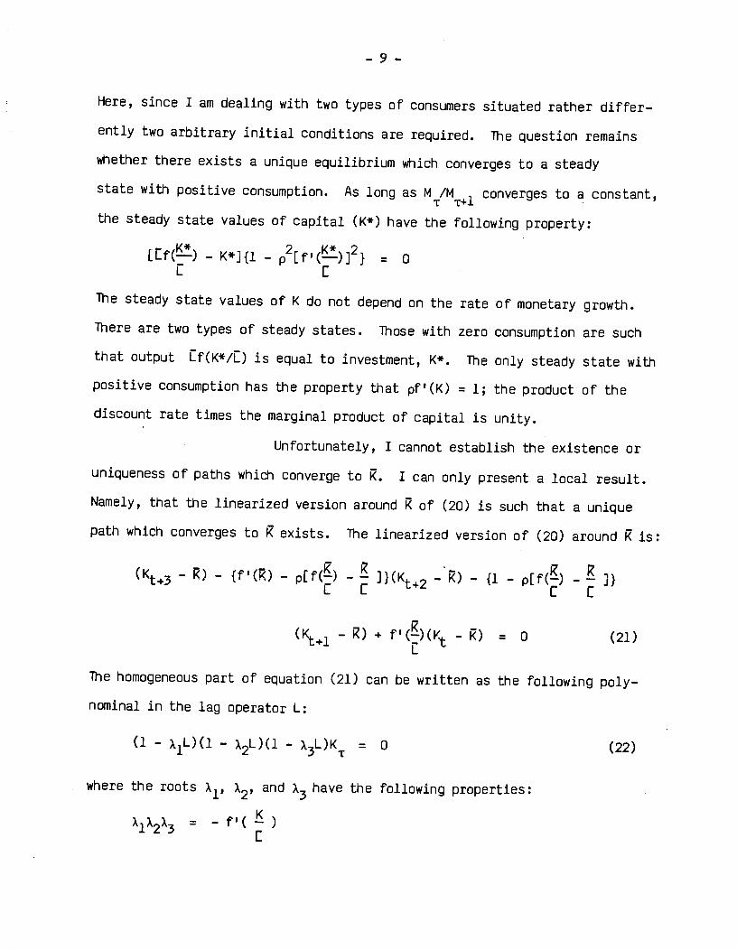
-9-

Here, since I am dealing with two types of consumers situated rather differ-

ently two arbitrary initial conditions are required. The question remains

whether there exists a unique equilibrium which converges to a steady

state with positive consumption. As long as M/M1 converges to a constant,

the steady state values of capital (K*) have the following property:

LEf() — K*]{l — p2[f'()]2} = 0C

The steady state values of K do not depend on the rate of monetary growth.

There are two types of steady states. Those with zero consumption are such

that output Cf(K*/C) is equal to investment, K*. The only steady state with

positive consumption has the property that pf'(K) = 1; the product of' the

discount rate times the marginal product of capital is unity.

Unfortunately, I cannot establish the existence or

uniqueness of paths which converge to R. I can only present a local result.

Namely, that the linearized version around R of (20) is such that a unique

path which converges to R exists. The linearized version of' (20) around R is:

(K3 - R) - {f'(R) - p[f() - ))(K -R) - {l -

p[f()-

(Kt 1- R) - = 0 (21)+

L

The homogeneous part of equation (21) can be written as the following poly—

nominal in the lag operator L:

(1 — A1L)(l—

X2L)(l—

x3L)K = 0 (22)

where the roots A2, and A3 have the following properties:

=

— 10 -

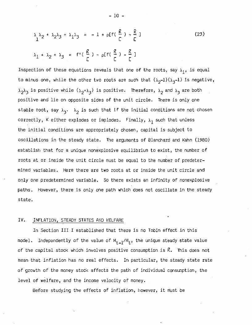
XX2+X2X3+XlX3 = -1+p[f'()-] (23)1 c

R R RX1 X2+ A3 = f'(—) -p[f'() -—3

C £

Inspection of these equations reveals that one of the roots, say A1, is equal

to minus one, while the other two roots are such that (x2—l)(x3—1) is negative,

is positive while (x2+x3) is positive. Therefore, A2 and A3 are both

positive and lie on opposite sides of' the unit circle. There is only one

stable root, say A3. A2 is such that if the initial conditions are not chosen

correctly, K either explodes or implodes. Finally, A such that unless

the initial conditions are appropriately chosen, capital is subject to

oscillations in the steady state. The arguments of Blanchard and Kahn (1980)

establish that for a unique nonexplosive equilibrium to exist, the number of

roots at or inside the unit circle must be equal to the number of predeter-

mined variables. Here there are two roots at or inside the unit circle and

only one predetermined variable. So there exists an infinity of nonexplosive

paths. However, there is only one path which does not oscillate in the steady

state.

IV. INFLATION, STEADY STATES AND WELFARE

In Section III I established that there is no Tobin effect in this

model. Independently of' the value of Mt+l/Mt, the unique steady state value

of the capital stock which involves positive consumption is R. This does not

mean that inflation has no real effects. In particular, the steady state rate

of growth of the money stock affects the path of individual consumption, the

level of' welfare, and the income velocity of money.

Before studying the effects of' inflation, however, it must be

— 11 —

ascertained that an inflationary path is consistent with the government's

budget constraint (14). I will assume that the government lets the money

stock grow at the rate m so that M/M1 = 1 -i. m. With the new money, the

government buys capital which it redistributes in lump sum fashion. These

lump sum redistributions affect none of the conditions used to derive (20).

So the amount of' capital held by the government can be arbitrarily set to some

constant.

I now compute the rate of' inflation which corresponds to a given rate of

growth of money. Equation (17) establishes that the steady state rate of'

inflation, ii, is given by:

P CTT+l = = (24)T CT

T

where, in the steady state, neither C nor CT_i depend on T. Therefore, using

(18):

Mlir = l+m (25)

The rate of' inflation is equal to the rate of monetary expansion. Note that

the model is quite consistent with the rate of' return dominance of' capital

over money in the steady state. The rate of return of' the former is

[(l/p) — 1], while that of the latter is —m.

By (24), the ratio of consumption on the date of financial transactions

to consumption in the f'ollowing period is: (l+m)/p; it rises as inflation

rises. Therefore, inflation distorts the intertemporal consumption deci-

sions. It leads people to consume more right after they withdraw money and

less in later periods.5 The rate of deflation which is such that inter—

temporal consumption decisions are optimal from the point of view of' society

is [(lip) — 1]. As Friedman (1969) proposed, the rate of' deflation must be

— 12 —

equal to the discount rate. This result was also obtained by Jovanovic (1982)

in a model in which money is held for transactions purposes but in which

people, while picking the timing of their visits to the financial intermedi-

aries optimally, do not pick their consumption path optimally. Here, it can

be shown as follows: consider a social planner who wants to maximize:

t[jflT + (1 - cz)1nCT] (26)Tl T T

subject to:

KK = Ef( ) - n(C + CT) - nB (27)T E T T

where a is a weight between zero and one. This social planner maximizes a

convex combination of' the utilities of both types of consumers subject to

society's budget constraint. The plan which maximizes (26) satisfies:

- C—1-a T

and:

KCT = pf'( _) C (28)T+l E

In the steady state in which pf'(K/C) isequal to one, consump—

sion is constant. Indeed, this is precisely what occurs in the decentralized

economy with money as long as, in (7) t+l't is equal to one. This in

turn requires that m be equal to [1 — (l/p)] as claimed.

However, there is a problem in sustaining the equilibrium with K = R when

m is equal to El — (l/p)]. This problem arises because at this equilibrium

money and capital have the same rate of return. Therefore households would

prefer to withdraw money at the beginning of' their lives in the amount equal

to the present discounted value of their income. Then they would avoid all

— 13 -

visits to their bank and associated transactions costs. This would result in

no capital being available in this model with 100% reserves. It may well be

the case that, with a smaller reserve requirement, the equilibrium would be

sustainable. In any event, note that, as long as m is just slightly bigger

than —[(lip) — 1], the equilibrium of this model is essentially equal to the

Pareto optimum and does induce people to hold R units of' capital.

Inflation induces people to consume less in the period in whith they do

not go to the bank. Therefore, M/P1, which is equal to this consumption,

falls. However, surprisingly, in this model, M/P actually rises with infla-

tion. This result is undoubtedly due in part to the fact that people do not

go to the bank more often when inflation rises. It emerges because even though

people want to reduce M IF , they must increase M /P to ensure that infla—T Tl T t

tion does not reduce M /P too much. The result can be established by notingT T+l

that equation (18) says that M/P is proportional to consumption in the period

in which people visit the financial intermediary. By equation (19), this con-

sumption does indeed rise with inflation.

V. THE NONNEUTRALITy OF MONETARY POLICY

The main purpose of this paper is to study conditions outside the steady

state. First, it will be established that a wide variety of monetary policies

(or open market operations) affect aggregate output. This is the consensus

view of textbooks, such as Branson (1979). However, this view has recently

been challenged by a variety of' authors (e.g., Wallace (1981), O-am1ey and

Polemarchakis (1982)). These authors have shown that in models in which money

is held only for its rate of return characteristics, open market operations

are neutral. Admittedly the premise of these models —— that money is not rate

of return dominated by other assets —— appears to be a bad description of

— 14 -

free—market economies as we know them. The proof that open market operations

can affect output in the economy of this paper is straightforward. Consider a

base path for money and taxes: {M} and {T}, then an equilibrium sequence of

capital {K} must satisfy (21). Consider any one of these equilibria.

Now consider a slightly different financial policy for the government.

At t, unexpectedly, the government purchases some extra capital by issuing

units of' money. Then, at T, the government engages in the reverse transaction:T—1 K

it sells c II f'( —- ) / units of capital. Therefore, the path of' taxesTt £

remains unchanged, but between t and T the path of money is replaced by {M + c}.I K.T

After T, the path of money is given by: {M + c[l -P1 f'( —-)] / Pt}.T i=t

Then, it is clear from (21) that if, in the new equilibrium, capital remains

unchanged from {K} at t and t+1, it will have to be different from Kt+2 at

t+2; monetary policy affects output.

The intuition behind this result is as follows. Suppose the open market

operation has no effect on prices. Then, the paths of consumption will be

unaffected. However, the people who visit the bank at t will not want to

demand the increased amount of' money balances. If, instead, any rate of

inflation after t is affected by the open market operation, then by (7)

someone will change their consumption path. Finally, suppose that only the

price at t is affected by the government's change of financial policy. Then

the consumption of those who visited the bank at t—1, which is given by

Mt1/Pt will be affected. So the nonneutrality of' open market operations

hinges crucially on the fact that not everyone visits the bank on the day of

the operation. This is, in fact, a striking feature of the U.S. institutional

setup.

I am not just interested in establishing that monetary policy is non—

neutral. Instead, I want to characterize their effect. I am unable to do so

— 15 —

for general policies and general production functions. Instead, the rest of

this section is devoted to simulating various monetary policies under addi-

tional assumptions.

First, I will assume that the production function is Cobb—Douglas, and I

will normalize the aggregate labor endowment to be equal to one. Therefore:

= K1 (29)

Moreover, I will assume that a = 0.25, and that p = 0.99. This hii rate

of' discount is appropriate since people visit financial intermediaries often.

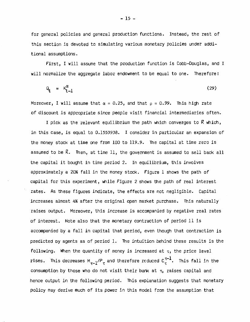
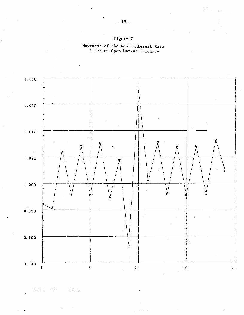
I pick as the relevant equilibrium the path which converges to R which,

in this case, is equal to 0.1553938. I consider in particular an expansion of

the money stock at time one from 100 to 119.9. The capital at time zero is

assumed to be R. Then, at time 11, the government is assumed to sell back all

the capital it bought in time period 2. In equilibrium, this involves

approximately a 20% fall in the money stock. Figure 1 shows the path of

capital for this experiment, while Figure 2 shows the path of real interest

rates. As these figures indicate, the effects are not negligible. Capital

increases almost 4% after the original open market purchase. This naturally

raises output. Moreover, this increase is accompanied by negative real rates

of interest. Note also that the monetary contraction of period 11 is

accompanied by a fall in capital that period, even though that contraction is

predicted oy agents as of period 1. The intuition behind these results is the

following. When the quantity of money is increased at 'r, the price level

rises. This decreases M 1/P and therefore reduced Cr1. This fall in the

consumption by those who do not visit their bank at -r, raises capital and

hence output in the following period. This explanation suggests that monetary

policy may derive much of its power in this model from the assumption that

— 16 —

those people who visited the bank at T—l do not change their pattern of' bank

visits in response to inflation at T. How much people who had not scheduled

a visit to their intermediary at -r would reduce their consumption in

response to inflation at T if' they were free to pick the timing of these

visits optimally, is an open question which deserves further research.

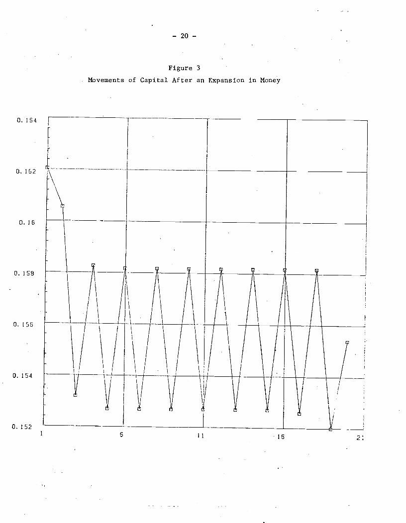
Unfortunately, the figures show that capital converges very slowly to

the steady state and that the negative root has important effects on the

dynamics of' the economy. For purposes of comparison, I also simulate the

effects from a once and for all expansion of money in period one to 119.9 from

100. This monetary expansion is then followed by the lump sum distribution of

the purchased capital. Figure 3 shows the resulting path for capital. What

is striking about this path is that the expansion of capital in the early

periods is almost identical to the expansion in Figure 2. Monetary policy

understood here as financial policy has about the same power as an expansion

in money which is unaccompanied by new government assets.

Before concluding this section, it is worth noting that if' the rate of'

-monetary expansion is changed unexpectedly once and for all at t, the path of'

capital is unaffected. Suppose that before t, M÷1/M was equal to (1+rn).

Then, before the change in rates of' monetary growth, (21) asserts that the

evolution of the capital stock was given by:

K K K KK = Ef( - p2ft( )f'( ){f(—) - K ] (29)-r+3 -r+1

Now, suppose that at t, it is announced that from now on MT+l/MT will be given

by (1+m*). Then the evolution of capital from t+3 on is still given by (29),

and the original values of' Kt+i and Kt+2 are still equilibrium values of'

capital.

— 17 -.

VI. CONCLUSIONS

The model of this paper is a modest step towards the construction of'

tractable and realistic general equilibrium models capable of shedding light

on the effects of nonsteady—state monetary changes. Its major advantage is

that people's motive for holding mpney is explicitly that money is used for

transactions. In particular, in those periods in which households do not

visit their banks, they are faced with an extreme version of' the "Clower

Constraint"; they must pay for their purchases with money carried over from

the previous period. This ensures that monetary policies which expand money

and prices, reduce the real consumption of those households which do not visit

their financial intermediary on the day of' the monetary expansion. This fall

in consumption raises capital and output in future periods.

1\ number of issues are raised by this paper. First, an important

question is to what extent the power of monetary policy would be diluted if

people timed their visits to intermediaries optimally. Associated with this

question is the question of whether people in fact do significantly alter the

interval during which they refrain from visiting their bank as events change.

The framework of this paper can also hopefully be used to study the

effects of various institutional setups on macroeconomic activity. In

particular, it should be capable of' shedding some light on the difference

between commodity standards, fractional reserve standards and the 100%

reserves standard of this paper.

0.17

0. 153

0. 16

0. 155

0. 15

0. 145

0. 14

—18—

Figure 1

Movements of Capital after an Open Market Purchase

I 6 11 16 21

— 19 —

Figure 2

Movement of the Real Interest RateAfter an Open Market Purchase

1. 030

1.060

1. 040

1.020

1.003

980

0. 963

0. 9401 6 ii 16

.

1

0. 154

0. 1(2

0. 16

0. 158

0. 156

0. 154

0. 152

— 20 —

Figure 3

Movements of Capital After an Expansion in Money

6 11 16

— 21 —

FOOTNOTES

1Primes denote first derivatives, while double primes denote second

derivatives.

2The analysis assumes that the holdings of money by household i from

t to t#l are nonnegative. Here this is guaranteed by the fact that nega-.

tive holdings of money would induce negative consumption and hence utility

equal to minus infinity. However, it labor income were paid in the form of

money, the constraint that monetary holdings be nonnegative might become

binding.

3This condition requires that capital be held in positive amounts at

4For simplicity, ignore the transaction costs incurred by the govern-

ment when it engages in an open market operation.

5mis has been noted also by Jovanovic (1982). This effect is likely

to be even more pronounced on consumer expenditure when there are durable

goods, and consumer expenditure can be different from consumption. In this

paper, consumption and consumer expenditure coincide by assufnption.

- 22 —

REFERENCES

Blanchard, Olivier Jean and Charles M. Kahn, "The Solution of Linear Differ-

ence Models under Rational Expectations," Econonietrica, 48, No. 5, July

1980, pp. 1305—12.

Baumol, William J., "The Transactions Demand for Cash: an inventory theoretic

approach," Quarterly Journal of Economics, 66, November 1952, pp. 545—56.

Branson, William, Macroeconomic Theory and Policy, 2nd edition, Harper & Row,

New York, 1979.

thamley, Ohristophe and Heraklis Polemarchakis, "Asset Markets, Returns and

the Neutrality of' Money," Mimeo, September 1981.

Friedman, Milton, The Optimum Quantity of' Money and Other Essays, Chicago,

Aldine, 1969.

Grandcnont, Jean—Michel and Yves Younes, "On the Efficiency of a Monetary

Equilibrium," Review of Economic Studies, 40, April 1973, pp. 149—65.

Hansen, Lars Peter and Kenneth Singleton, "Generalized Instrumental Variables

Estimation of Nonlinear Rational Expectatiàns Models", 1982, forthcoming

in Econometrica.

Helpman, Elhanan, "Optimal Spending and Money Holdings in the Presence of

Liquidity Constraints," Econometrica, 49, No. 6, November 1981, pp.

1559—70.

Jovanovic, Boyan, "Inflation and Welfare in the Steady State," Journal of

Political Economy, 90, No. 3, June 1982, pp. 561-77.

Lucas, Robert E.,, Jr., "Equilibrium in a Pure Currency Economy," 18, No. 2,

April 1980, pp. 203—20.

Mankiw, N. Gregory, "The Permanent Income Hypothesis and the Real Interest

Rate," Economic Letters, 7, 1981, pp. 307—11.

— 23 -

Stockman, Alan C., "Anticipated Inflation and the Capital Stock in a Cash—

in—Advance Economy," Journal or Monetary Economics, 8, November 1981,

pp. 387—93.

Tobin, James, "The Interest Elasticity of the Transactions Demand for Cash,"

Review of' Economics and StatIstics, 38, No. 3, August 1956, pp. 241—7.

Townsend, Robert M., "Asset Market Anomalies: a monetary explanation," MimeO,

1982.

Wallace, Neil, "A Modigliani—Miller Theorem for Open-Market Operations,"

American Economic Review, 7, No. 3, June 1981, pp. 267—74.