6. Pillar Gridding

The generation of the structural model is done in a process called Pillar Gridding. Pillar Gridding is a unique concept in Petrel where the faults in the fault model are used as a basis for generating the 3D grid. Several options are available to customize the 3D grid for either geo-modeling or flow-simulation purposes. Pillar Gridding is the process of making the ‘Skeleton Framework’. The Skeleton is a grid consisting of a Top, a Mid and Base skeleton grid, each attached to the Top, the Mid and the Base points of the Key Pillars. There is a close relationship between the Fault Modeling process and the Pillar Gridding process. The user might need to go back and work on the fault modeling process in order to solve problems appearing in the gridding process. These problems could have been found during the fault modeling but not visible until in the gridding process. The relation between the Fault Modeling process and the Pillar Gridding is an iterative process with which the user should spend some time in order to attain a grid of good quality and high cell orthogonality. The result from the Pillar Gridding is a set of pillars both along the faults but also in between faults. The grid has no layers, only a set of pillars with user given X and Y increments between them (like a pincushion). The layering is introduced when making horizons and zones. Before starting Pillar Gridding, a series of checks need to be performed to ensure that the fault modeling process is complete. There are some things that we recommended you to check before you start with the Pillar Gridding process: 6.1 Before Pillar Gridding

• In a 3D window, display all faults in the fault model, • Ensure that all faults intersecting are connected properly. Laterally connected

faults should have a shared (grey) Key Pillar, • Check and see that a fault is not represented twice in the model, • The transition between all neighboring pillars should be smooth, • Faults represented by Key Pillars should not cross each other. Make sure to

display the faults in the 3D window with the Toggle fill turned on. Check all faults and ensure that the triangulated surface between the different Key Pillars is not crossing.

6.2 Create a New 3D Grid

To create pillar gridding, follow the steps:

• Start the process of creating a new 3D Grid, • Go to Structural Modeling item in the Process Diagram tab, • Double click on Pillar Gridding tab in the Process Diagram, • The Pillar Gridding process dialog box pops up. A 2D window will

automatically open and display the faults model in map view, as shown in Fig. 6.1,

83

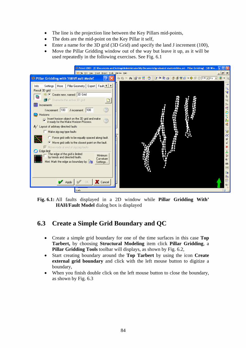
• The line is the projection line between the Key Pillars mid-points, • The dots are the mid-point on the Key Pillar it self, • Enter a name for the 3D grid (3D Grid) and specify the land J increment (100), • Move the Pillar Gridding window out of the way but leave it up, as it will be

used repeatedly in the following exercises. See Fig. 6.1 Fig. 6.1: All faults displayed in a 2D window while Pillar Gridding With’

HAH/Fault Model dialog box is displayed 6.3 Create a Simple Grid Boundary and QC

• Create a simple grid boundary for one of the time surfaces in this case Top

Tarbert, by choosing Structural Modeling item click Pillar Gridding, a Pillar Gridding Tools toolbar will displays, as shown by Fig. 6.2,

• Start creating boundary around the Top Tarbert by using the icon Create external grid boundary and click with the left mouse button to digitize a boundary,

• When you finish double click on the left mouse button to close the boundary, as shown by Fig. 6.3

84

Fig. 6.2: Creating simple grid boundary for Top Tarbert while Pillar Gridding Tools toolbar is displayed

85

Fig. 6.3: Boundary is created in a 2D window

6.4 Create a Segment Grid Boundary To create a segment grid boundary, follow the steps:

• Delete the simple grid boundary you just created by selecting the boundary (under the Fault Model) and hitting delete on your keyboard.

• Display one of the time surfaces in the input tab of Petrel Explorer in the 2D window. This will be used as a guide when digitizing the boundary.

• Start by making faults, on the left side of the area, part of the boundary. Use the Set Select/Pick mode to mark a fault as shown in Fig. 6.4.

• Click on the Set part of grid boundary icon. • Continue the boundary from fault to fault (digitizing points in between) on the

south, east, and north sides of the boundary. • Select the Create Boundary segment icon as shown in Fig. 6.5. • Click on a shape point on a fault to start digitizing the boundary from. • Digitizing the boundary between the two faults so it matches the surface

displayed. You can digitize anyway you like but you can not cross faults. • Click on a shape point on the second fault to close the boundary segment.

Fig. 6.4: Digitizing faults on the left side of Top Tarbert

86

Fig. 6.5: Making selected faults part of a segment boundary

87

6.5 Inserting Directions and Trends

• Look for the overall fault pattern in the 2D window. In this case the major faults are oriented North-South. Give the main fault(s) aligned North-South a red J direction. With the Select/Pick mode icon select the line between the shape points to select the fault and press Set J-direction icon as shown in Fig. 6.6

• Give a perpendicular fault a green I direction, selecting the faults in the same manner as above and pressing Set I-direction icon as shown in Fig. 6.7,

Fig. 6.6: Main Fault NS 1 as J-direction displayed in a 2D window

88

Fig. 6.7: Main Fault NS 1 as I-direction displayed in a 2D window

• Press Apply in the process window and observe the changes in the miskeleton grid. See Fig. 6.8,

• Continue to set directions to all major faults in the project, • Insert a trend in the I direction (green) between two J direction faults (red),

See Fig. 6.9, • Press apply and observe how the cells are aligned along the trend line, • Make sure that the direction and trend alignment are ok by conducting a QC of

the mid-skeleton grid in the 2D window. Add directions on faults and trends to

d

refine the mid-skeleton grid.

89

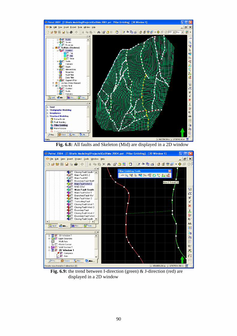
Fig. 6.8: All faults and Skeleton (Mid) are displayed in a 2D window

Fig. 6.9: the trend between I-direction (green) & J-direction (red) are displayed in a 2D window

90

6.6

etry),

the

etry

6.7

• Double click on the intersection folder and toggle on show pillars in the style tab settings window. See Fig. 6.12

Pillar Gridding

After the Boundary has been defined and the 2D cell geometry tuned to the point of acceptability (trends and directions may be applied to help tune the 2D cell geomthe 3D grid can be constructed. The result of this construction is the Skeleton, which is a series of pillars, one for the corner of each cell. Top, middle and base skeleton grids are used to view these pillars easily in the X-Y dimensions. The integrity ofpillars themselves can be viewed in an I or J intersection plane. Under the Pillar Geometry tab in the Pillar Gridding process window, toggle off ‘Curved’ for the ‘Non-Faulted Pillars’. This will create a simpler 3D Grid geomwith less chance for problems as shown in Fig. 6.10.

Fig.6.10: The Pillar Geometry for Pillar Gridding dialog box

Quality Control (QC) of the Skeleton Grid

• Activate the project (make bold) in the Models tab of Petrel Explorer. • Open the Skeleton folder in the newly created 3D grid. • Perform a visual check of the grids individually in the 3D window, look for

spikes and irregularities. The comments below describe what to look for. • Display the Key Pillars from the fault model to locate the problem. • In the 3D window display a J-intersection from the “Intersections” folder.

Click on the name to make it active. See Fig. 6.11

91

Fig. 6.11: QC

for Top Skeleton by Grid J-direction 1 displayed in a 3D window

Fig. 6.12: QC for Top Skeleton by Grid J-direction 1 displayed in a 3D window while Settings for Intersection are shown

92

6.8

6.9

king

n e

other fault or boundary, See Fig. 6.13,

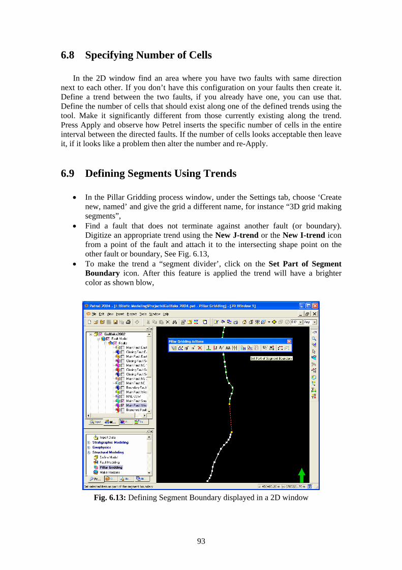
Fig. 6.13: Defining Segment Boundary displayed in a 2D window

Specifying Number of Cells

In the 2D window find an area where you have two faults with same direction next to each other. If you don’t have this configuration on your faults then create it. Define a trend between the two faults, if you already have one, you can use that. Define the number of cells that should exist along one of the defined trends using the tool. Make it significantly different from those currently existing along the trend. Press Apply and observe how Petrel inserts the specific number of cells in the entire interval between the directed faults. If the number of cells looks acceptable then leave it, if it looks like a problem then alter the number and re-Apply.

Defining Segments Using Trends

• In the Pillar Gridding process window, under the Settings tab, choose ‘Create new, named’ and give the grid a different name, for instance “3D grid masegments”,

• Find a fault that does not terminate against another fault (or boundary). Digitize an appropriate trend using the New J-trend or the New I-trend icofrom a point of the fault and attach it to the intersecting shape point on th

• To make the trend a “segment divider’, click on the Set Part of Segment Boundary icon. After this feature is applied the trend will have a brighter color as shown blow,

93

• Display the skeleton grid colored with dsettings for the skeleton folder in the pr

ifferent colors for the segments. Open evious 3D grid, and check show solid

ig. 6

as segments. Do the same for the “3D grid making segments”. See Fig. 6.14

F .14: The skeleton grid colored with different colors for the segments are displayed in a 2D window

94

Setting Undefined Faults 6.10

• Select the fault or part of the fault.

Fig. 6.15: Fault displayed in a 2D window while Pillar Gridding Action tools are shown

• Click on the Set No Fault icon. • The selected part of the fault will become dotted. See Fig. 6.15

95

6.11 Setting a Fault as "Not a Part of Segment Boundary"

• Select the fault or part of the fault. .

ill become grey. If the fault already has a J-ig. 6.16

Fig. 6.16: Fault displayed in a 2D window while Pillar Gridding Action tools are shown

• Click on the Set No Boundary icon• The selected part of the fault w

direction, it will show as a solid line, with a dark red color. See F

96