Embed Size (px)
Citation preview

Piezoelectric Energy Harvesting From
Flutter
By
Soroush Norouzi
B.Sc. (Mechanical Engineering), University of Tehran, 2009
Thesis Submitted in Partial Fulfillment
of the Requirements for the Degree of
Master of Applied Science
in the
School of Engineering Sciences
Faculty of Applied Sciences
Soroush Norouzi 2013
SIMON FRASER UNIVERSITY
Spring 2013
All rights reserved. However, in accordance with the Copyright Act of Canada, this
work may be reproduced, without authorization, under the conditions for “Fair Dealing.” Therefore, limited reproduction of this work for the purposes of private study, research, criticism, review and news reporting is likely to be in accordance with the
law, particularly if cited appropriately.

ii
Approval
Name: Soroush Norouzi
Degree: Master of Applied Science
Title of Thesis: Piezoelectric Energy Harvesting From Flutter
Examining Committee:
Chair: Dr. Erik Kjeang Assistant Professor Mechatronic Systems Engineering
Dr. Siamak Arzanpour Senior Supervisor Assistant Professor Mechatronic Systems Engineering
Dr. Gary Wang Supervisor Professor Mechatronic Systems Engineering
Dr. Mehrdad Moallem Internal Examiner Professor Mechatronic Systems Engineering
Date Defended/Approved:
December 11th , 2012

iii
Partial Copyright License

iv
Abstract
With the increasing need for alternative sources of energy, a great deal of
attention is drawn to harvesting energy from ambient vibration. These
vibrations may be caused by fluid forces acting upon a structure. When a
flexible structure is subject to a fluid flow, it loses stability at a certain flow
velocity and starts to vibrate. This self-induced motion is called flutter where
energy is continuously transferred from the fluid to the structure. In this study
a piezoelectric film sensor is used as a fluttering object, to convert the motion
to electrical energy, and the energy harvesting capacity of the proposed
concept is investigated. An experimental setup, composed of data acquisition
methods, is designed and the findings are validated by original test data. The
results are also compared to similar literature and it is concluded that the
proposed energy harvesting technique meets the requirements of the
intended application.
• Keywords: Flow-Induced Vibrations, Flutter, Piezoelectricity, Energy Harvesting

v
Dedication
To Mom, Dad, Brother

vi
Acknowledgements
First and foremost, I send my deepest gratitude to my family; the absolute
source of love and support, who have always had the most faith in me, even
when I had the least.
I would like to thank my supervisor, Dr. Siamak Arzanpour, for affording me
the opportunity of working in his research group. He has taught me lessons, in
science and life alike, which I hold of utmost value. I am very grateful for all
his guidance and support, for this work could not have been completed
without them. I would also like to thank Dr. Gary Wang for the support and
care he offered me, both professionally and personally. I thank Dr. Mehrdad
Moallem, my examiner, for accepting to read and evaluate this thesis
Special thanks go to my friend and companion, Maryam Hamidirad, who has
been the light in the dark, and the warm in the cold. I express my highest
appreciation for her love and support.
I thank my friends and lab mates. I hold dearest the time we shared, and the
talk.
Finally, I would like to thank me, who kept at it.

vii
Table of Contents
Approval ................................................................................................................ ii Partial Copyright License ..................................................................................... iii Abstract ................................................................................................................ iv Dedication ............................................................................................................. v Acknowledgements .............................................................................................. vi Table of Contents ................................................................................................ vii List of Figures ...................................................................................................... ix
Chapter 1: Introduction ................................................................................... 1 Motivation ............................................................................................................. 1
Literature Review .................................................................................................. 3 Energy Harvesting From Fluid Flow .............................................................. 3
Flutter: a Flow-Induced Vibration .......................................................................... 6 Contribution........................................................................................................... 7 Thesis Outline ....................................................................................................... 9
Chapter 2: Theoretical Approach to Piezoelectric Energy Harvesting From Flutter .............................................................. 10
Linear Modeling of Flutter ................................................................................... 10
Solution Method .................................................................................................. 13 Piezoelectric Energy Harvesting ......................................................................... 17
Backward Coupling ..................................................................................... 21
PVDF Patch System Identification ...................................................................... 23 Assessing the Significance of Backward Coupling ..................................... 26
Validity of the Linear Model ................................................................................. 27 Nonlinear Flutter Analysis ................................................................................... 29
Frequency Analysis .................................................................................... 34
Chapter 3: Experimental Approach to Piezoelectric Energy Harvesting From Flutter .............................................................. 37
Wind Tunnel Experiments ................................................................................... 37 Data Acquisition Method for Measurement of Output Voltage .................... 39
Experimental Results of the Generated Power ........................................... 43 Observations on Actual Flutter Behaviour ........................................................... 49 Electromechanical Conversion of PVDF Patch ................................................... 51
Chapter 4: High-Speed Video Large Deflection Vibrometry ....................... 55 Examining the Deflection Measurement Method................................................. 59
Preliminary Investigation ..................................................................................... 60 Measurement Results for Tip Deflection and Output Voltage ............................. 62
Chapter 5: Conclusion and Future Directions ............................................. 64 Conclusion .......................................................................................................... 64 Future Directions ................................................................................................. 65

viii
Works Cited ...................................................................................................... 66

ix
List of Figures
Figure 1: Schematic of a Fluttering Cantilever ................................................... 11
Figure 2: Typical Beam Deflection ..................................................................... 11
Figure 3: Schematic of the Energy Harvester Patch .......................................... 17
Figure 4: Schematic diagram of the Circuit ........................................................ 19
Figure 5: Schematic Changes in Voltage versus R values ................................ 20
Figure 6: Schematic Changes in Power versus R values .................................. 21
Figure 7: PVDF Mounted on the Shaker Head................................................... 24
Figure 8: Tip Velocity data from the Shaker Experiment .................................... 25
Figure 9: Approximation of the Damping Ratio .................................................. 26
Figure 10: Tip Velocity for Open and Closed Circuit Configurations .................... 27
Figure 11: Calculated Critical Velocity for Different Number of Modes ................ 28
Figure 12: Divergence of the linear model ........................................................... 29
Figure 13: Tip Deflection for Flow Velocities below Critical Velocity .................... 31
Figure 14: Tip Deflection for Large Initial Condition for ........................... 31
Figure 15: Simulation Results for Flutter Vibrations at ..................... 32
Figure 16: Simulation results for the output voltage ............................................. 33
Figure 17: Changes of Output Voltage RMS with Load Resistance..................... 33
Figure 18: Changes of Output Power RMS with Load Resistance ...................... 34
Figure 19: Frequency Content of the Tip Deflection ............................................ 34
Figure 20: Tip deflection for simulation without the first mode ............................. 35
Figure 21: Frequency Content of the Output Voltage .......................................... 36
Figure 22: Theoretical Electromechanical Transfer Function ............................... 36
Figure 23: Experimental Setup for Investigation of PVDF Flutter......................... 38
Figure 24: DAQ Circuit for Voltage Measurement of the PVDF ........................... 39
Figure 25: Time Domain Output Voltage Data ..................................................... 40

x
Figure 26: Time Domain Output Voltage over a Larger Sampling Period ............ 40
Figure 27: RMS of the Measured Voltage Signal ................................................. 41
Figure 28: FFT of the Voltage Signal ................................................................... 41
Figure 29: Total Output Voltage of the PVDF ...................................................... 42
Figure 30: Frequency Verification of the Theoretical Output Voltage ................... 42
Figure 31: Output Voltage vs. Load Resistance for Different Lengths ................. 43
Figure 32: Voltage-Resistance Curve Fitting Results vs. Data ............................ 44
Figure 33: RMS of Generated Power vs. Load Resistance ................................. 45
Figure 34: Energy Harvesting Capacity for Different Lengths .............................. 45
Figure 35: Main Flutter Frequency for Different PVDF film lengths...................... 46
Figure 36: Optimal Resistance at Various PVDF Lengths ................................... 46
Figure 37: Comparison of Driving Power and Harvested Power .......................... 48
Figure 38: Energy Harvesting Ratio ..................................................................... 48
Figure 39: Instance of the Fluttering of the PVDF ................................................ 49
Figure 40: Corrected Theoretical Tip Deflection .................................................. 50
Figure 41: Corrected Theoretical Voltage vs. Experimental Results .................... 51
Figure 42: Transfer functions at Different Load Resistance Values ..................... 52
Figure 43: Transfer Functions Corrected for Test Load Resistance .................... 53
Figure 44: Double Corrected Output Voltage vs. Experimental Result ................ 53
Figure 45: Locating the Approximation Points on the Beam ................................ 56
Figure 46: Parameterization Of the Approximated Beam .................................... 58
Figure 47: Approximated Tip Displacement DFT vs. Actual Tip Displacement FFT .............................................................................. 59
Figure 48: Average DFT for the Variations of All Segments ................................ 61
Figure 49: Convergence of the Calculated Frequencies of the Peaks ................. 61
Figure 50: Calculated Frequency Content of Tip Deflection ................................ 62
Figure 51: Video Vibrometry Output Voltage vs. Experimental Data ................... 63

1
Chapter 1: Introduction
Motivation
In light of the drastic advancements in electronics technology throughout the
past couple of decades, a paradigm change has been happening in various
fields of engineering. A major distinction between the new generation of
measurement systems and their predecessors is the built-in intelligence as a
result of employing a sensor network, controllers and data transmission
apparatus. Thanks to light-weight and low-powered radio transmitters,
sensors can now be placed in remote locations and provide live data on
various mechanical properties of systems such as pressure, temperature, etc.
The wireless nature of these measurement devices is in accordance with the
demand for minimizing the use of material, reducing cost and saving energy.
However to take full advantage of these opportunities a reliable long-lasting
source of electric power must be available to keep these devices operating.
This is challenging because the wireless sensor networks are basically
intended for use in remote locations where the wiring needed for power
distribution is not available. Therefore the concept of localized power sources
is considered as a potential solution.
One possible substitute for central powering in sensor networks and
data transmission units is to use batteries. The disadvantage of this solution,
however, is that batteries have a limited lifespan and it is not always feasible
or even possible to have access for battery replacement or recharging after
they are in place. In gas pipelines, for example, neither central nor battery
power transmission is desirable because cutting the surface of the pipe to
pass wires or provide access for battery replacement will require extra safety

2
considerations to avoid any leakage. On the other hand, such a system will
require frequent maintenance which would be very expensive in the case of
pipelines that extend for hundreds of kilometres. These issues will make
batteries an unfeasible solution for applications that are meant to perform over
extended periods of time.
An alternative approach is to locally generate the needed electricity
relying on the ambient energy. This approach has been adopted in wrist
watches and some other cases for a long time and is called Energy
Harvesting. Since a major application of sensors is measuring mechanical
properties, some form of mechanical energy usually exists in the surroundings
that can be harnessed and converted to electricity by means of an
electromechanical transducer. The generated electrical power may then be
used directly to power the equipment or to help recharge the battery to
prolong its lifespan. For example, when pressure is being measured on a
pipeline, the fluid within the pipe carries a kinetic energy due to its flow. This
motion can be transferred to an electromechanical transducer, where energy
conversion can happen.
There are a number of options for converting mechanical motion into
electricity. Electromagnetic conversion is one of the most common
techniques, where the motion of a coil inside a magnetic field induces an
electric current in the coil. This method is widely used in power plants as well
as low-power energy harvesters [1], but one disadvantage is the design
complexity, of such systems with multiple parts, e.g. coil, magnet, slider, etc.,
required to work in harmony. This will lead to more difficult design which is
also not suitable for small size applications. Another approach is using
piezoelectric materials that generate an electric field in response to an applied
mechanical stress. These materials are widely used in vibration-based energy
harvesters due to their simplicity of use and high power generation capacity
[1]. In general, the choice of a proper transduction method depends mainly on
the mechanics of the problem in terms of the ambient energy and how it can
be transferred to the transducer.

3
In this thesis we aim to find an energy harvesting solution where the source of
ambient energy is a moving fluid. To that end, a review of the relevant
literature is first conducted to understand the characteristic of the situation and
identify different potential approaches for energy conversion and their cost
and benefit. This knowledge will then be used to proceed to designing the
energy harvester.
Literature Review
Energy Harvesting From Fluid Flow
Windmills are well-known clean energy power generators that have been
around for many years to convert wind power to electricity. These devices are
expensive and are only economically recommended where sufficient wind
power is available and preferable not located close to where people live.
Moreover, windmills have significant maintenance costs and as a result they
will be only allowed to operate when the efficiency is above a threshold. In an
attempt to find an alternative for windmills, Adamko and DeLaurier [2] and
McKinney and DeLaurier [3] proposed the idea of an oscillating-wing windmill
(wingmill). This device consists of a series of airfoil-shaped “wings” that are
sequentially attached and placed in a fluid flow. The flapping of these wings
due to the fluid flow is then converted to rotary motion that is transferred to an
electromagnetic generator. Despite the original idea to use this device as a
wind power generator, it can also work with water in rivers where building a
dam is not feasible. Ly and Chasteau [4] demonstrated that the wingmill can
achieve efficiency equal to a vertical axis wind turbine [5].
It is to be noted that the portion of the entire available power that wind
turbines capture is limited to Betz limits [6] of 33% and 59% for vertical and
horizontal axis configurations, respectively [7]. Therefore, for the purpose of
energy harvesting where ample ambient energy is not always available, only
low-powered energy harvesters can be made using the conventional turbine-
generator configuration. For example, Weimar et al. [7] employed an
anemometer to transfer wind power to a small-scale generator and provide an

4
energy source for low-power autonomous sensors. Their design was able to
achieve up to 80% conversion efficiency with output powers limited to 700
microwatts. Although the main goal of the wingmill was to compete with
conventional wind turbines, it was one of the first approaches to use flow-
induced vibrations as a source for electricity generation. Meanwhile, the
majority of energy harvesting research consists of vibration-based devices
that work with an external oscillatory vibration with low amplitude and constant
frequency [8]. Flow-induced vibrations could be used as a source of
mechanical energy in situations where a fluid flow is present
In the past, flow-induced vibrations were considered unwanted and
destructive in design problems such as aircraft wings or long bridges. It is
because the interactions between the structure and its surrounding fluid can
grow to such large amplitude vibrations that over time can lead to serious
damage and failure of the structure. Despite this harmful nature of flow-
induced vibrations, there have been attempts to benefit from the huge energy
content of these vibrations to generate electricity.
The energy-harvesting eel is one the methods, proposed by Allen and
Smits [9] and Taylor et al [10], for fluid-induced vibration energy harvesting.
This device comprises of a flexible piezoelectric polymer film placed in a
wake, generated from an upstream bluff body. The turbulences caused by the
object vibrate the film. Due to the piezoelectric effect, electric charge is
generated in response to the stresses associated with this vibration. This
energy-harvesting concept can provide an electricity source to power remote
sensors. This idea has already been patented by Carrol [11] while researchers
are still trying to improve the device's electrical output and efficiency. Another
interesting design of a flow-induced vibration energy-harvesting device is
“windbelt” which has recently been patented and manufactured by Humdinger
Wind Energy, LLC [12]. A windbelt is a properly tensioned flexible belt placed
in airflow. The main difference between this design and the energy harvesting
eel is the three-dimensional deformation of the flexible belt. A similar device is
also proposed by Vortex Oscillating Technology, Ltd. [13].

5
Another source of vibration which has not been widely considered for energy
harvesting is flutter. Flutter initiates when a fluid flow passes over a flexible
structure (e.g., a cantilever beam) and the fluid pressure force on the structure
causes it to deflect. Then, the elasticity of the structure counters these forces
and creates a dynamic interaction with the fluid. If the stiffness of the structure
suffices to resist substantial deformation, the system can stay in balance. For
higher flow-induced forces, however, the deformations can grow to a point
that the geometry of the flow field is significantly altered, thus complicating the
dynamics of the system. At a certain critical flow velocity, the structure loses
its stability and starts to vibrate. Once the stability is lost, the oscillations will
constantly be fuelled by the energy of the moving fluid. This type of persistent
vibration is referred to as flutter, and can be seen in various scenarios from
the waving motion of flags, to the buzzing reeds in a Clarinet. The self-
induced and continuous nature of flutter creates an opportunity for energy
harvesting in situations where a constant ambient flow is present. A recent
study by Tang et al., [14] investigated the energy transfer between the plate
and the surrounding fluid flow based on which they propose the concept of a
new energy-harvesting device, called “flutter-mill” [15]. In that study, however,
the flutter-mill benefits from an electromagnetic transduction scheme,
therefore sophisticated design and multiple parts are required. A different
design concept was introduced by Bryant and Garcia [16] by placing an airfoil
in a flow and transferring the flutter vibrations to a piezoelectric ceramic (PZT)
by means of linkages. Erturk et al. [17] performed an experimental study
investigating the output power and the effect of energy harvesting on the
flutter dynamics of the airfoil. The first one to use a simplistic design was
Kwon [18] who studied a T-shaped energy harvester that worked in a cross
flow orientation. This device used a PZT mounted on a larger substrate, so
that the fluttering would lead to power generation by the PZT.
Flutter seems to be a promising approach of energy harvesting for the
remote sensor networks that motivated this research study. To better benefit
from flutter in energy harvesting from fluid flow an investigation about the
phenomena and the parameter involved is essential.

6
Flutter: a Flow-Induced Vibration
The earliest literature on flutter is of the experiments conducted by Taneda
[19] who studied the flutter of hanging strips. He used linear models to
investigate the instabilities of strips in air flow. Later on, Datta and Gottenberg
[20] tried to propose a theoretical prediction of the critical velocity (minimum
flow velocity required for flutter to take place) in terms of strip dimensions
based on a similar series of experiments. Neglecting the nonlinearities in the
system, both of these studies combined Euler-Bernoulli and Slender Wing [21]
theories for modeling the structure and the fluid behaviour, respectively. They
found the linear model to be able to predict the stability threshold with
acceptable consistency with test data. In a more recent research, Lemaitre et
al. [22], motivated by their experimental observations, followed the same
theoretical approach to investigate the potential independence of the critical
velocity from strip length for long hanging strips. They found that critical
velocity decreases for longer strips until it reaches a final value. The first
group to study the plates in a vertical/horizontal configuration were Kornecki et
al. [23] who, instead of using slender wind theory, assumed a potential flow
with zero circulation and added a distribution of vorticity on the plate using
Theodorsen's theory [24] to account for the two-dimensional flow. Meanwhile,
Argentina and Mahadevan [25] investigated the flutter mechanism of
cantilevered plates in axial flow by means of a simplified analytical model
based on Theodorsen's theory. To further advance the fluid modeling, Balint
and Lucey [26] employed a Navier-Stokes solver in their attempt to provide a
treatment for human snoring, which is the flutter of the palate. They found a
mechanism of irreversible energy transfer from the fluid to the structure
supporting the self-induced and continuous nature of this phenomenon.
The flutter stability conditions of structures have been theoretically and
experimentally studied in a number of research projects, benefiting from the
accuracy linear models can provide for determining the critical velocity.
Analyzing the three-dimensional stability, Shayo [27] concluded that a flag of
infinite span is more stable than a finite one, which was contrary to what Datta
and Gottenberg [20], Lemaitre [22] and Lighthill [28] had found. This

7
discrepancy was re-examined by Lucey and Carpenter [29] from a theoretical
standpoint, and revealed to have stemmed from the assumptions Shayo had
made to simplify the calculations. Further, Eloy and Souillez [30] performed an
analytical study with no limiting assumptions and showed that the system is in
fact more stable for smaller plate spans; a statement consistent with the
results of Argentina and Mahadevan [25].
Although linear Euler-Bernoulli model is proven accurate for studying
the critical velocity, it is not capable of describing the behaviour of the
structure after flutter happens. This is because the large deflections
associated with flutter render the behaviour highly nonlinear. Hence, Tang et
al. [31] accounted for the nonlinearity by adding a condition of inextensibility to
the beam, and used numerical vortex lattice model [21] to calculate the
aerodynamic forces. Their work was theoretically extended by Attar et al. [32]
to include nonlinearities in the vortex lattice model as well. Further, Tang and
Païdoussis [33] introduced material damping of the Kelvin-Voigt type [34] to
the nonlinear model.
A general understanding on flutter, stability analysis and modeling
approaches is made possible through an early monograph published by
Dowell [35]. Later, Païdoussis [36] summarized the flow-induced vibrations
and instabilities, providing a more in-depth understanding of the various
problems in as well as covering different areas of the subject.
Contribution
The goal of this project is to develop a novel energy harvesting solution,
where the mechanical energy of a fluttering cantilever is converted to
electrical energy by means of a piezoelectric transducer. A low-cost
Polyvinylidene Fluoride (PVDF) film sensor, which is often used as strain
gauges and contact microphones for vibration or impact detection, is used as
the energy harvester. These sensors are constructed of a layer of PVDF film,
sandwiched between two electrodes meant for picking up the electric charge

8
the film produces under mechanical stress. When immersed in a wind flow of
adequate speed, a cantilevered PVDF sensor will flutter and thus generate a
varying charge distribution in the PVDF film. If the electrodes are connected to
an electrical load, the variations in the charge distribution cause an alternating
current in the circuit. The properties of the current depend on various
parameters such as the vibration frequency and amplitude, and the
electromechanical conversion characteristics of the PVDF film.
The first step towards realizing our concept of flutter-based energy
harvester is to understand the physical nature of flutter, as well as
piezoelectric materials. Therefore an extensive literature review is conducted
on fluid-structure interactions and piezoelectric energy harvesting. The
theoretical basis provided by this study resulted in a mathematical model of
the system, capable of determining the critical velocity, fluttering
characteristics of the PVDF patch and the output voltage. A set of
experiments was then designed based on the critical velocity predicted by the
math, to verify the energy harvesting capacity of the proposed design.
The output power of the energy harvester was measured for various
load resistances, using a data acquisition method specific to the needs of our
experiment, and the optimal load resistance and the maximum attainable
harvesting capacity was determined. Although the experiments validated the
critical velocity and the frequency response calculated by the model, the flutter
of the PVDF sensor was drastically stronger than the expected magnitude.
This discrepancy along with the main focus of this project to propose a new
energy harvester concept, called for an alternative approach for assessment
and correction of the theoretical results based on empirical methods. These
techniques were able to reproduce the experimental data.
Finally, inspired by the great potentials of the empirical methods a
novel video vibrometry system was designed for measuring large deflection
vibrations. Using a high-speed video camera, the fluttering PVDF was filmed
and the picture was analyzed by means of an innovative algorithm to measure
the frequency and the magnitude of the vibration. The results were also

9
combined with the empirically identified piezoelectric characteristics of the
PVDF film sensor to estimate the output voltage of the system. These
calculations lead to an improved accuracy in determination of the output
power, while creating an alternative measurement technique for application
where laser vibrometry is not possible.
Thesis Outline
Chapter 2 explains the theory of flutter in flexible structures, and derives the
mathematical model of the energy harvester by considering piezoelectric
properties for the vibrating structure. The first phase of experiments and the
result comparison is covered in Chapter 2 as well. In Chapter 3, the
experimental approach for measurement of the energy harvesting capacity of
the system is presented. The results of this study are compared to the findings
of Chapter 2 in order to verify the theoretical data. Also the errors in
determination of flutter dynamics and electromechanical conversion is
discussed, and corrections are made in order to improve the theoretical
results. Inspired by these empirical corrections, Chapter 4 discusses an
innovative technique as an alternative to laser vibrometry in case of high
deflection vibrations. Finally, the conclusive remarks and the future directions
of this work are covered in the 5th Chapter.

10
Chapter 2: Theoretical Approach to Piezoelectric Energy Harvesting From Flutter
In order to design a flutter-based piezoelectric energy harvester we must first
understand the nature of flutter and the parameters that contribute to it. This
knowledge will be essential for studying the feasibility of flutter power
harvesting, demonstrating the power generation potential and identifying the
key design parameters. In this chapter, we first create a general
understanding of flutter by presenting the linear model. This model is then
used as the basis for the theoretical analysis. The effect of electromechanical
transduction is also discussed by introducing the piezoelectric effect into the
equations. To run the simulations using the linear model, the physical
properties of the PVDF beam are first measured by experimental system
identification. These properties are used in the solution of the linear model
and the results are presented and discussed. Due to the shortcoming of the
linear model, an improvement is sought by means of considering the large
deformations that create a nonlinear vibration. The results of this simulation
method are presented at the end of this chapter.
Linear Modeling of Flutter
Figure 1 illustrates the simplest fluid-structure configuration leading to
occurrence of flutter, where a cantilever beam is subjected to a laminar wind
flow. The schematic in Figure 1 is used to derive a mathematical model of
flutter and discuss the various aspects of this phenomenon.

11
Figure 1: Schematic of a Fluttering Cantilever
Based on the Euler-Bernoulli linear model, the differential equation associated
with the system in Figure 1 is of the form [35]:
(1)
In Equation (1) spatial and temporal differentiation is shown by prime and dot,
respectively. is the transverse deflection of the beam (Figure 2), which is a
function of both location on the beam and time. The other parameters in
Equation (1) are the beam’s density ( cross-sectional area , flexural
rigidity ( ) and the fluid load ( ).
Figure 2: Typical Beam Deflection
Several methods could be used to determine the value of including
Slender Wing Theory [21], Theodorsen's Theory [24], Vortex Lattice Method
[37], etc. Each of these methods provides a degree of accuracy while each
has its own shortcomings in terms of complication and computation intensity.
w
x
12
Our application is energy harvesting from a regular fluid flow that can be found
in the surroundings of typical industrial applications, Therefore the flow can
usually be assumed inviscid, incompressible and laminar. Here, we follow the
approach of Lemaitre et al. [22] which uses the slender-wing theory for its
validity within the conditions of engineering non-aviation problems. According
to Slender Wing Theory, the pressure forcing due to the fluid flow can be
calculated as [20]:
(2)
In Equation (2), and are the flow velocity and the fluid-added mass,
respectively. The fluid added-mass depends on the geometry of the surface of
the plate and for a flexible beam it is [22] with and being
the fluid density and the beam's width, respectively. Each term in Equation (2)
represents a different influence of the flow on the vibrating beam. The first
term is the centrifugal force due to the flow of the fluid over the curved parts of
the beam. The second term is a Coriolis force since each of the beam’s
infinitesimal parts are somewhat rotating relative to the flow which has a linear
velocity. Finally the last term is the inertial term due to the motion of fluid
particles along with the transverse deflection of the cantilever beam.
As inferred by Equation(2), fluid forces are dependent upon the value
of the flow velocity . Below a certain fluid velocity, called the critical velocity,
the forcing terms are not strong enough to overcome the flexural rigidity and
the inertia of the beam to start the vibrations. In fact, these forcing terms help
stabilize the system so that every oscillation induced by an initial condition or
forcing fluctuations will be damped by these forces. As the flow velocity is
increased towards and beyond the critical value , the influence of these
terms becomes significant and the damping of the system becomes negative,
thus resulting in instability of the system.

13
The first step in analyzing flutter is to determine the critical velocity. Once this
property of the system is found, further investigation can be performed on the
post-flutter behaviour of the beam.
Solution Method
Calculating the critical velocity is possible via solving the partial differential
equation of motion for the transverse deflection. The candidate solution of any
second order differential equation is in exponential form of , with a
complex angular frequency . The imaginary and real parts of the solution
determine the oscillation frequency and the damping of the system,
respectively. Hence, the critical velocity is the value of flow velocity at which
the damping of the system becomes negative.
Due to the complexity of the differential equations associated with
flutter, analytical solution would be very complicated and beyond the scope of
this thesis. Moreover, there exist no exact solutions for the case of nonlinear
differential equations. Approximate numerical methods, on the other hand,
take advantage of the highly-developed processing powers of modern
computers, while maintaining acceptable accuracy. The most common
technique is to decompose the transverse deflection of the beam into spatial
and temporal components, as demonstrated in Equation(3). This method is
known as Galerkin’s decomposition method.
(3)
Here, the spatial functions, are the shape functions that must satisfy
the boundary conditions of the physical problem, and the temporal functions
are generalized coordinates determining the participation weight of
each of the shape functions. Galerkin’s method is similar to the well-known
separation of variables technique in solving partial differential equations. The
difference, however, is that the spatial and temporal functions are both solved

14
for in the latter, while in the former, the spatial functions are assumed
beforehand. The decomposition then reduces the partial differential equation
to a set of ordinary differential equations, with the temporal functions
remaining as the unknowns.
Any set of functions that satisfy the boundary conditions of the
differential equation can be chosen as shape functions. Nevertheless, it is
common practice (and quite convenient) to consider the in vacuo mode
shapes of the cantilever beam, since they are easily calculable and meet the
boundary conditions. These mode shapes are the eigenfunctions of the Euler-
Bernoulli beam equation without considering the fluid effects. To solve these
in vacuo differential equations, we can use separation of variables. Without
the pressure term in Equation(1), it can be solved as follows:
Where is a constant because and are functions of and , respectively,
and thus no general equality can exist between functions of and unless
both sides of the equality are constant. Therefore a set of trigonometric
differential equations is derived from the above equality:
These equations represent the temporal and spatial components of the in
vacuo vibration of the beam. Solving the first equation results in the mode
shapes of the beam, each corresponding to a frequency determined by
solution of the second equation. Solving the spatial equation for yields:

15
(4)
In order to determine the coefficients of each of the trigonometric functions in
Equation (4), we need to apply the boundary conditions of the cantilever beam:
• Zero deflection and slope at the clamped end:
• Zero moment and shear force at the free end:
By considering these conditions, Equation (4) can be rewritten as:
(5)
Equation (5) shows the definition of the beam’s in vacuo mode shapes. The
parameters of this equation are also found by applying the boundary
conditions as:
(6)
(7)
These mode shapes are mutually orthogonal meaning that:
(8)
Now that the shape functions of Galerkin's expansion are known, the
transverse deflection of the beam can be written in terms of the mode shapes
and generalized coordinates. Prior to this step, however, we must determine
the number of modes we need for our approximation, since infinite number of
values can be calculated from Equation (6), each yielding a different mode
shape of the vibration. The number of the required modes depends on the

16
problem and the proper level of accuracy. Since more accuracy is attainable
by using a higher number of modes, we can iteratively raise the number of
modes until the solution reaches a plateau with an acceptable variation.
Substituting Galerkin’s expansion in Equation(1) decomposes the
equation into spatial and temporal terms. Moreover, in order to convert the
partial differential equations to a set of ordinary differential equations, we can
take advantage of the orthogonality of the mode shapes. In this procedure the
equation resulting from substitution of Equation(3) into the Euler-Bernoulli
equation is multiplied by and then integrated over the length of the beam.
This leads to a set of ordinary temporal differential equations of the form:
(9)
Where:
Equation (9) can be used to solve for the generalized coordinates of the
system. These equations define an N-mode system and the general solution
of this type of equations is:
(10)
Each mode has a complex frequency of . The occurrence of flutter is
because the real part of one of these frequencies becomes negative. The
other modes have positive damping and do not contribute to steady-state
vibrations. Once the mechanical parameters of the problem such as the

17
density and flexural rigidity of the beam are known, we can proceed to
calculating the critical velocity of flutter.
Piezoelectric Energy Harvesting
The next modeling step is to include the piezoelectricity of the fluttering beam.
Piezoelectric sensors and energy harvesters vary in their forms and
configurations. Figure 3 shows a unimorph PVDF film sensor, where a single
layer of the polymer is mounted on a substrate of flexible material. Another
common type of these transducers is bimorph PZT sensors that consist two
layers of piezoelectric ceramics mounted on a substrate material. The
flexibility required by our application dictates a lightweight and compliant
patch, therefore PVDF film sensors are often designed in unimorph
configurations, including a flexible Mylar substrate (Figure 3).
Figure 3: Schematic of the Energy Harvester Patch
The PVDF converts the mechanical deformations into a voltage difference,
which is collected by a couple of electrodes attached to either faces of the
PVDF film. To evaluate the produced power, we should first consider the
piezoelectric constitutional relations. These relations specify the coupling
between the strain and the electric field. The fundamental equation for
piezoelectric material is [38]:
(11)
18
Where , and are the electric displacement, piezoelectric effect and
the permittivity at constant stress, and and are the axial stress in the
piezoelectric film and the voltage magnitude of electric field, respectively.
Using
, that relates permittivity at constant strain to
permittivity at constant stress based on the Young Modulus of the piezo layer
( ), Equation (11) can be rewritten as:
Considering where is the maximum distance from
the beam’s neutral axis ( ), and:
The equation for the produced current is:
(12)
It is common in the literature to consider PVDF both as a voltage or current
source and interchanging between the two configurations is possible through
Thevenin-Norton equivalencies [1]. The film sensor is connected to a circuit
with the load resistance as shown in Figure 4. Note that in this study, the
internal capacitance of the PVDF ( ) is accounted for in the
equations and thus is considered encapsulated in the PVDF package. the
generated voltage is:
(13)

19
Figure 4: Schematic diagram of the Circuit
Finally, combining Equations (12) and (13), the differential equation for the
produced voltage is derived as:
(14)
Equation (14) is a first-order linear differential equation and can be used to
calculate the output voltage of the energy harvesting system, once the
mechanical deformations of the beam are found. A number of points can be
implied from this equation:
Importance of Vibration Frequency: Since a time derivative of the
transverse deflection of the beam is present in the right-hand side of the
equation, vibrations with small tip deflection but high frequency can
theoretically produce voltages comparable to ones with large displacements
and low frequencies.
Effect of the Load Resistance: By changing the load resistance, the
generated voltage of the system can be changed. If we assume Equation (15)
in a general form with left as the only parameter:
Cp
RL
PVDF
20
(15)
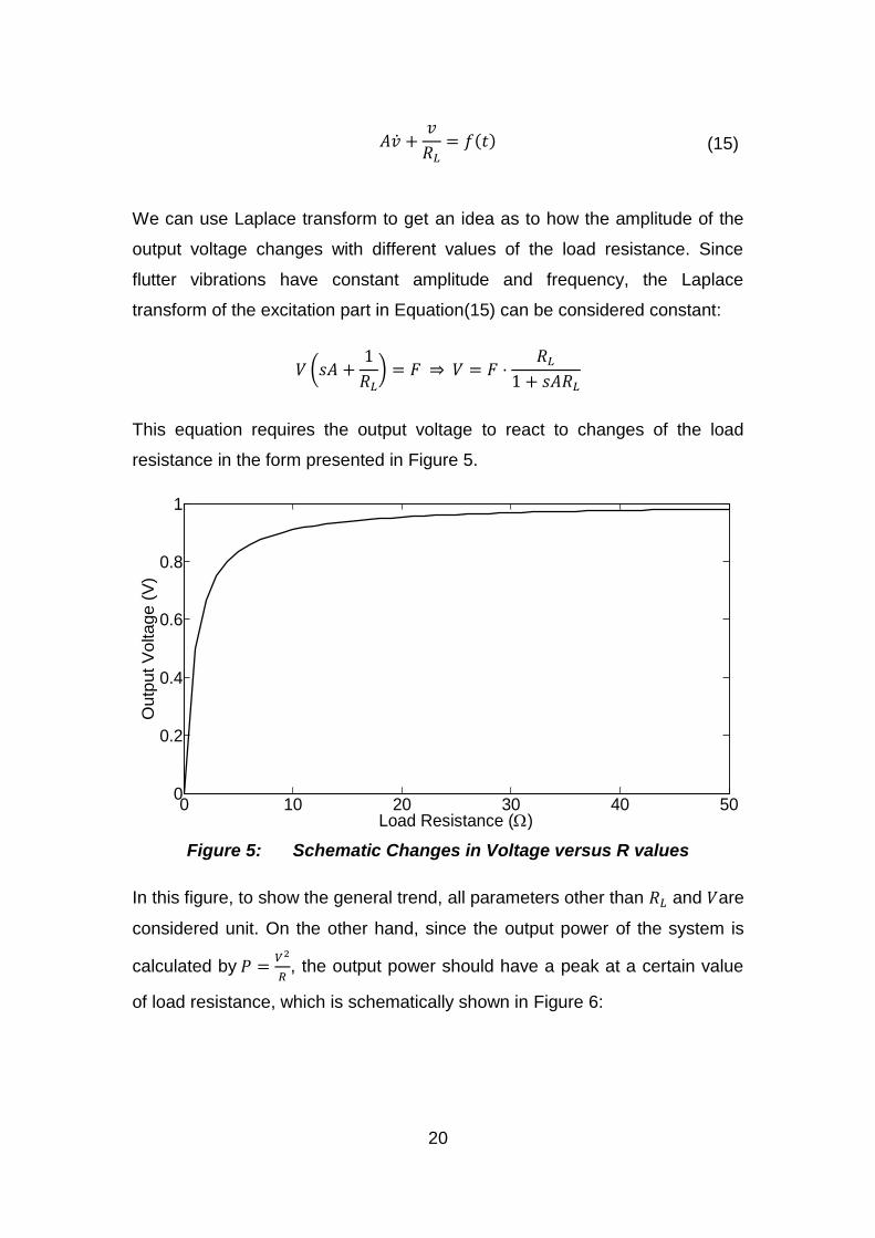
We can use Laplace transform to get an idea as to how the amplitude of the
output voltage changes with different values of the load resistance. Since
flutter vibrations have constant amplitude and frequency, the Laplace
transform of the excitation part in Equation (15) can be considered constant:
This equation requires the output voltage to react to changes of the load
resistance in the form presented in Figure 5.
Figure 5: Schematic Changes in Voltage versus R values
In this figure, to show the general trend, all parameters other than and are
considered unit. On the other hand, since the output power of the system is
calculated by
, the output power should have a peak at a certain value
of load resistance, which is schematically shown in Figure 6:
0 10 20 30 40 500
0.2
0.4
0.6
0.8
1
Load Resistance ()
Outp
ut V
oltage (
V)

21
Figure 6: Schematic Changes in Power versus R values
This peak corresponds to an optimum load where the output power of the
system is maximized. The location of 3the point is determined impedance
matching between the load resistance and the PVDF.
Backward Coupling
The mechanical and electrical behaviours of the piezoelectric transducer are
coupled in a way that the produced voltage introduces a tension,
subsequently, and inflicts a bending moment into the composite strip. This
effect is known as backward coupling. To introduce the piezoelectricity to the
equations, the stiffness term of Equation (1) can be expressed for the bending
moment of the beam as:
Where is the bending moment throughout the composite beam. If the
width of the PVDF is denoted as , this bending moment can be calculated:
0 10 20 30 40 500
0.05
0.1
0.15
0.2
0.25
Load Resistance ()
Outp
ut P
ow
er
(V)

22
In this equation, and are the distances of bottom and top layers of the
piezoelectric film from the neutral axis, respectively. The electric field and
tension are related as [38]:
(16)
Now considering the fact that is relating the electric field to the
voltage ( ) and the thickness of the PVDF layer, since the mechanical strain is
a function of the beam's radius of curvature, the total bending moment within
the piezoelectric layer will be:
This added moment ) is applied on the part of the beam to which the
electrodes are attached. If electrodes are placed between and along the
length of the beam, should be multiplied by the voltage
effect term, where is the Heaviside step function [39]. Here, it is
considered that the electrodes cover the whole beam thus the added moment
becomes:
The first term is bundled within the first term in Equation (1), and the second
term, when twice differentiated with respect to x, adds a forcing term:
Where is the Dirac delta function. The added forcing tem changes the
dynamics of the system based on the output voltage of the PVDF, coupling
the equations of motion and voltage generation.

23
PVDF Patch System Identification
Although electrical and mechanical properties of PVDF are accessible in the
literature, since the patch being used for this study is meant for commercial
rather than research purposes, no information on structural details of the film
sensor is available. However, it is necessary that certain specifications are
determined so the beam can be modeled with acceptable accuracy. Therefore
the mechanical properties of the path, including flexural rigidity, mass per unit
length and structural damping, are evaluated through a system identification
procedure.
Mass per unit length of the PVDF beam is easily measurable by means
of a scale. To this end, a piece of the PVDF patch was cut
and found to weigh. . Therefore the mass per unit length of the
beam is . In order to determine the flexural rigidity,
however, a proper method is needed since the high compliance of the patch
makes it inaccurate to simply observe the tip deflection caused by a certain
tip-mass and calculate the stiffness.
Based on the Galerkin’s decomposition of the in vacuo differential
equation, Equation (17) is derived for calculating the natural frequencies of the
beam based on the flexural rigidity and the mass-per-unit-length of the beam.
Hence, if the frequencies are known, the unknown stiffness can be derived
from this equation.
(17)
The natural frequencies of the cantilever beam can be measured with an
experiment, where the base of the beam is mounted on a shaker head and is
excited by a range of frequencies. Fully clamped boundary condition is
maintained by gluing the PVDF film to a Plexiglas fixture, which is bolted to
the shaker head (Figure 7).

24
Figure 7: PVDF Mounted on the Shaker Head
The response of the beam as the deflection of the tip is measured using a
Polytec PSV-400 Scanning Vibrometer. Equipped by a video camera and a
scanning laser, this measurement device provides a video image of the object
to be analyzed. The point of vibrometry can be located using a computer
mouse. The tip velocity is then graphed versus the excitation frequency which
is input from the shaker controller. When the frequency sweep of the shaker
coincides with the natural frequencies of the beam, a peak in the response
curve is observed due to resonance. Figure 8 shows the experiment result for
excitation frequencies of 5-100 Hz.
The two peaks visible in Figure 8 correspond to the frequencies of the
first two natural vibration modes of the beam. Nonetheless, these frequencies
are the damped natural frequencies of the beam. The system is damped by
both the material damping and the ambient air, which affects the observed
resonance frequency:

25
Figure 8: Tip Velocity data from the Shaker Experiment
is the damped natural frequency. Since the damping coefficient ( ) is
different for each of the vibration modes, the measurements have to be
corrected so that the undamped natural frequency can be calculated. The
empirical method for estimating the damping coefficient is to find the peak
value for each mode and draw a horizontal line so that it intersects with the
curve at two points with velocities equal to the peak velocity divided by
[40]. The frequency difference of these two points is then used to approximate
the damping coefficient by:
In Figure 9 we show this procedure for the frequency response of the tip
velocity. Hence:
0 20 40 60 80 1000
100
200
300
400
500
600
Frequency (Hz)
Tip
Velo
city (
mm
/s)

26
Figure 9: Approximation of the Damping Ratio
Considering the length of the beam to be , the flexural rigidity of the
beam is calculated from Equation (17) to be:
Assessing the Significance of Backward Coupling
Although all transducers exhibit backward coupling due to their piezoelectric
nature, the stress generated by this phenomenon might not be significant
enough to change the movement of the system. In order to investigate
whether or not backward coupling is influential in our setup, we used the
shaker test to see if the vibrations of beam would be different when a load is
connected to the output of the PVDF. Therefore, the same base excitation
experiment is performed for the two cases of open and closed circuits and the
tip deflection plotted for comparison. As it is apparent from Figure 10, the
backward coupling does not change the motion of the beam significantly and
can be neglected in simulations of flutter.
0 20 40 60 80 1000
100
200
300
400
500
600
=0.053102,d=12.7057
=0.049021,d=77.8125
Frequency (Hz)
Tip
Velo
city (
mm
/s)

27
Figure 10: Tip Velocity for Open and Closed Circuit Configurations
Validity of the Linear Model
Now that we have the actual mechanical properties of the experimental setup,
the temporal equations defined by Equation (9) can be used to calculate the
critical velocity. As mentioned earlier, Equation (9) defines a set of
differential equations. Each of these equations results in one of the temporal
functions ( ). In order for flutter to happen, the damping of one of the
vibration modes becomes negative. By substituting in
Equation (10), however, we can detect the onset of flutter by solving for the
roots of the system of differential equations. When the damping of one of
these roots becomes negative, the frequency of that mode grows and
dominates the flutter vibration. By solving these characteristic equations we
can determine the critical velocity that causes the damping to become
negative. The shortcoming of this method is that due to the coupled nature of
the equations, finding the characteristic equation for higher mode numbers
would be a complicated task. On the other hand, we have employed the
differential equation solvers available in MATLAB™. These solvers are based
on state-space representation and provide the user with the tools and controls
needed for approaching any type of differential equation, linear or nonlinear.
0 20 40 60 80 1000
100
200
300
400
500
600
Frequency (Hz)
Tip
Velo
city (
mm
/s)
Closed Circuit
Open Circuit
28
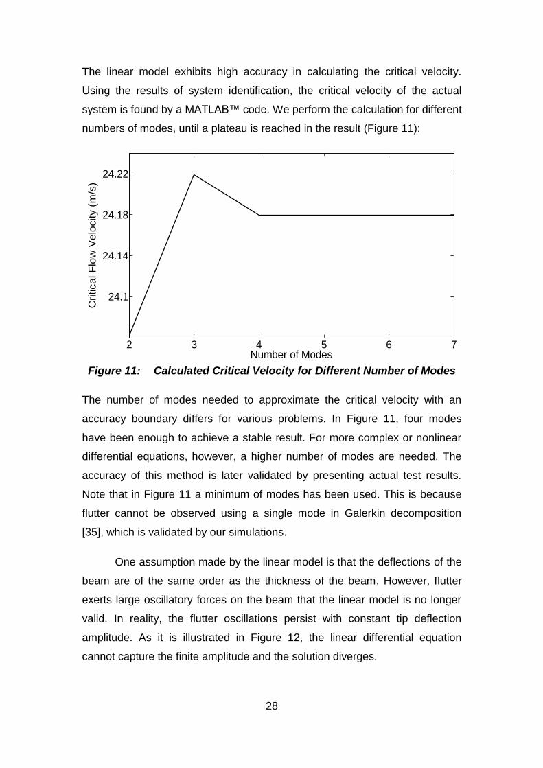
The linear model exhibits high accuracy in calculating the critical velocity.
Using the results of system identification, the critical velocity of the actual
system is found by a MATLAB™ code. We perform the calculation for different
numbers of modes, until a plateau is reached in the result (Figure 11):
Figure 11: Calculated Critical Velocity for Different Number of Modes
The number of modes needed to approximate the critical velocity with an
accuracy boundary differs for various problems. In Figure 11, four modes
have been enough to achieve a stable result. For more complex or nonlinear
differential equations, however, a higher number of modes are needed. The
accuracy of this method is later validated by presenting actual test results.
Note that in Figure 11 a minimum of modes has been used. This is because
flutter cannot be observed using a single mode in Galerkin decomposition
[35], which is validated by our simulations.
One assumption made by the linear model is that the deflections of the
beam are of the same order as the thickness of the beam. However, flutter
exerts large oscillatory forces on the beam that the linear model is no longer
valid. In reality, the flutter oscillations persist with constant tip deflection
amplitude. As it is illustrated in Figure 12, the linear differential equation
cannot capture the finite amplitude and the solution diverges.
2 3 4 5 6 7
24.1
24.14
24.18
24.22
Number of Modes
Critical F
low
Velo
city (
m/s
)

29
Figure 12: Divergence of the linear model
Nonlinear Flutter Analysis
As the flutter vibration amplitude grows, the axial body tensions of the beam
come into play rendering the dynamics of the vibration [35]. Bending creates
axial tension that in return resists bending. The longitudinal stress term is –
where:
and are the length and the thickness of the beam, respectively. Adding the
tension term into the linear beam representation, the nonlinear equation of
motion can be derived as:
For the large deformations to be significant enough to influence the dynamics
of the beam, the tension forces have to be of comparable magnitude as the
excitation and resistance terms. By substituting this condition for the two
terms of stiffness and axial tension, we can find the threshold for the
0 0.1 0.2 0.3 0.4 0.5-30
-20
-10
0
10
20
30
Time (s)
Tip
De
fle
ctio
n (
mm
)

30
deflections to be considered large. If we assume to be of the same order
as , we can compare the orders of magnitude of the stiffness term and the
nonlinear tension term:
This shows that the transverse deflection of the beam has to be of the order of
the beam's thickness to lead to nonlinear flutter behaviour.
By applying Galerkin’s decomposition to the nonlinear equation, the
MATLAB™ solvers can be used to find the temporal functions and calculate
the tip deflection. The finite-amplitude oscillations of flutter are of the limit-
cycle form. This means that there is a second pseudo-stability point where the
amplitude of the vibration remains constant and the beam continues to
vibrate.
Note that in this modeling approach, the transverse deflection of the
beam is assumed to be constant along the width of the beam and therefore no
tension in -direction is considered. Also the tension model used is very
simple, but it is able to capture the post-flutter finite-amplitude oscillations.
More realistic and therefore complicated equations are derived and discussed
in [41], [42]. Since the focus of this study is to investigate the energy
harvesting capacity of the proposed concept, further complexity is avoided.
Experiments will be presented to evaluate the results of this model.
Without an initial condition, these equations do not yield any results. In
reality, the fluctuations in the flow initiate the instability of the system.
Therefore, an initial tip velocity triggers the instability of the system. For flow
velocities less than the critical velocity, the motion due to the initial condition is
damped by the fluid forces and does not lead to flutter. In this simulation, a tip
velocity from the order of excites a rather negligible vibration is the
system (Figure 13).

31
Figure 13: Tip Deflection for Flow Velocities below Critical Velocity
By increasing the magnitude of the initial condition, the system can be pushed
into a temporary flutter-like phase that due to insufficient flow energy, gets
eventually damped (Figure 14).
Figure 14: Tip Deflection for Large Initial Condition for
For fluid velocities higher than the critical velocity, the flutter vibrations of the
beam can be captured by the nonlinear model. In Figure 15 the system is
subjected to a fluid velocity of and the tip deflection is calculated. As it
0 0.1 0.2 0.3 0.4 0.5-0.8
-0.6
-0.4
-0.2
0
0.2
0.4
0.6T
ip D
efle
ctio
n (
mm
)
Time (s)
0 0.1 0.2 0.3 0.4 0.5-1
-0.5
0
0.5
1
1.5
2
2.5
Time (s)
Tip
Deflection (
mm
)

32
can be seen in this figure, the vibration amplitude grows to a maximum and
remains constant at that value. Note that the magnitude of tip deflections is
comparable to the length of the beam and is two orders of magnitude greater
than the thickness. This shows that the system can no longer be assumed
linear.
Figure 15: Simulation Results for Flutter Vibrations at
The equations of the piezoelectric effect are simultaneously solved along with
the equations of motion. The output voltage of the system can therefore be
calculated. Figure 16 shows calculation results of solving the voltage
differential equation for the load resistance of . The output voltage
changes with the load resistance. As previously shown in Figure 5, the output
voltage grows to a final value, therefore creating a peak in the power-
resistance curve (Figure 6). The results of the numerical solution are in
agreement with the trend anticipated by the general analytical solution. The
changes of output voltage with load resistance are demonstrated in Figure 17.
In this figure, the root mean square (RMS) of the output voltage approaches a
final value of . The power output of the system is also calculated
by .
0 0.1 0.2 0.3 0.4 0.5
-0.2
-0.1
0
0.1
0.2
0.3
Time (s)
Tip
Deflection (
mm
)

33
Figure 16: Simulation results for the output voltage
Figure 17: Changes of Output Voltage RMS with Load Resistance
As shown in Figure 18, there is a load resistance where the output power
reaches a maximum of . The optimal resistance, which depends on the
material properties of the piezoelectric transducer [1], has been . The
results show that the system is capable of generating enough power for
remote sensor networks [43].
0 0.1 0.2 0.3 0.4 0.5-2
-1.5
-1
-0.5
0
0.5
1
1.5
Time (s)
Ou
tput V
oltag
e (
V)
0 2 4 6 8 100
1
2
3
4
5
6
7
8
9
Load Resistance (M)
Ou
pu
t V
oltag
e R
MS
(V
)

34
Figure 18: Changes of Output Power RMS with Load Resistance
Frequency Analysis
The frequency content of the tip deflection can be found by applying the Fast
Fourier Transform (FFT) on the results presented in Figure 15.
Figure 19: Frequency Content of the Tip Deflection
Figure 19 shows the frequency content of the tip deflection as calculated by
the theoretical approach. In this figure, two frequencies are observed to be
prominent. The number of modes assumed in Galerkin decomposition affects
the number of the peaks we observe in the FFT. By changing the number of
modes in the solution it was observed that the frequency content is the same
0 2 4 6 8 100
5
10
15
20
25
Load Resistance (M)
Ou
pu
t P
ow
er
RM
S (
W)
0 50 100 150 200 2500
0.05
0.1
0.15
0.2
Frequency (Hz)
Ma
gn
itud
e (
mm
)

35
for three and four modes. For the case of two assumed modes the second
peak disappears from the result, leaving only one peak in the calculated
frequency content. Since there seems to be a missing peak from the
frequency content, we omit the first mode from the 3-mode simulation to see if
same result is obtained.
Figure 20: Tip deflection for simulation without the first mode
As it can be seen in Figure 20, flutter cannot be captured for the case where
the first mode is omitted. This means that although the first mode does not
appear in the frequency content of the tip deflections, it is necessary for flutter
to happen. The second mode corresponds to the first peak of the frequency
response, which is greater by one order of magnitude, and it is the main
component of flutter vibration. That is why the time domain changes of the
deflection are dominated by a single frequency and the third mode has not
been significant.
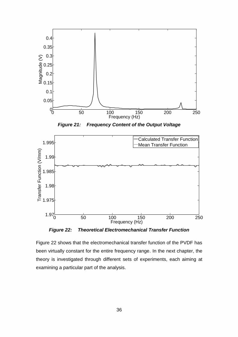
The frequency content of the output voltage is also calculated using
FFT. As is shown in Figure 21, the two peaks observed in the tip deflection’s
frequency content are present in the voltage signal at the same frequency
values. By dividing the output voltage by the tip deflection, we can calculate
the transfer function that converts the tip deflection (Figure 22).
0 0.1 0.2 0.3 0.4 0.5-0.25
-0.2
-0.15
-0.1
-0.05
0
0.05
0.1
0.15
Tip
Deflection (
mm
)
Time (s)
36
Figure 21: Frequency Content of the Output Voltage
Figure 22: Theoretical Electromechanical Transfer Function
Figure 22 shows that the electromechanical transfer function of the PVDF has
been virtually constant for the entire frequency range. In the next chapter, the
theory is investigated through different sets of experiments, each aiming at
examining a particular part of the analysis.
0 50 100 150 200 2500
0.05
0.1
0.15
0.2
0.25
0.3
0.35
0.4
Frequency (Hz)
Magnitude (
V)
0 50 100 150 200 2501.97
1.975
1.98
1.985
1.99
1.995
Frequency (Hz)
Tra
nsfe
r F
unction (
V/m
m)
Calculated Transfer Function
Mean Transfer Function

37
Chapter 3: Experimental Approach to Piezoelectric Energy Harvesting From Flutter
In this chapter, the theoretically calculated output voltage of the piezoelectric
flutter-based energy harvester is examined by experimental analysis. We first
explain the wind tunnel experiment designed to asses different parts of the
theoretical approach. Then the innovative data acquisition algorithm is
discussed, which is created to specifically make repeatable readings of the
output voltage of the wind tunnel test setup. Finally the results are presented
and compared to those obtained from the theoretical approach.
Wind Tunnel Experiments
In order to validate the results of the theoretical study, as well as to determine
the actual energy harvesting capacity of the proposed device, a wind tunnel
experiment was designed. In this experiment, we create an environment
where the output flow of the wind tunnel is used to excite the PVDF patch and
cause it to flutter. Figure 23 shows the experimental setup used in this study.
As it is shown in the figure, the PVDF patch is enclosed within a Plexiglas duct
which is attached to the outlet of a wind tunnel. The dimensions of this duct
are determined based on the calculated critical velocity obtained from the
theoretical study. Also some preliminary tests were done and a qualitative
knowledge on the behaviour of the vibrations was gained. The PVDF is
mounted in flag-like orientation so that it cannot be bent due to its own weight.
The first set of tests is conducted to investigate the role of flow velocity in the
dynamics of the system. In this phase, we observe the motion of the beam for
different values of flow rate in the wind tunnel. The flow rate of the wind tunnel

38
is adjusted by turning a knob that changes the angular frequency of the fan
driving the flow.
Figure 23: Experimental Setup for Investigation of PVDF Flutter
Higher flow velocities correspond to higher pressure difference between two
points in the flow. Therefore, a pressure sensor is employed to measure the
pressure difference between two fixed points on the wind tunnel prior to the
outlet. This value is then used in a proprietary spreadsheet of the wind tunnel
to calculate the flow rate and fluid velocity.
Similar to the predictions of the nonlinear model, for lower velocities,
the beam is steady and any disturbance is damped. As the flow speed is
raised, the disturbances become more influential and lead to temporary
fluttering. At the critical velocity, however, the vibrations can start with a
negligible initial excitation and fluttering will be continuous. In fact, since the
flow cannot be perfectly maintained at linear conditions, the fluctuations of the
flow can internally trigger the instability of the system. The flow velocity of the
experimental setup is in acceptable agreement with the predicted value as
resulted from the linear model. The PVDF beam lost its stability at
. The value calculated in Figure 11 is , which differs from
the actual test data by . The second step in the experimental analysis is to
measure the voltage of the fluttering PVDF to validate the theoretical data. In

39
this regard a data acquisition method is designed to measure the output
signals of the fluttering PVDF.
Data Acquisition Method for Measurement of Output Voltage
The same wind tunnel setup as Figure 23 is used for this part of the
experiments and the output voltage is measured by means of a National
Instruments Data Acquisition (DAQ) card. Since the load resistance
experienced by the PVDF influences its output voltage and power, the internal
resistance of the DAQ card ( ) needs to be isolated to avoid the
dependency of results on measurement device.
Figure 24: DAQ Circuit for Voltage Measurement of the PVDF
Therefore a characteristic resistor of is paralleled to the DAQ card
so the effect of the DAQ’s resistance is reduced to negligible. Figure 24 shows
the circuitry used for the experiments. We use MATLAB™’s Data Acquisition
Toolbox for saving and analysing the time domain voltage measured by the
DAQ card. Figure 25 shows the voltage reading of the DAQ card for a load
resistance of . As it can be seen in this figure, due to the erratic nature
of flutter, as well as the imperfections of the experimental setup to maintain a
laminar wake-free flow, the raw output voltage of the PVDF is not very
suitable for a repeatable reading to be possible (Figure 25). Sudden jumps
and slightly varying amplitude is observed in the alternating output voltage.
For longer sampling times, however, the voltage amplitude seems to have a
mean value subject to temporary changes (Figure 26). Therefore, we
designed a data acquisition program in MATLAB™ to read that data from the
DAQ card and calculate the RMS of the voltage signal every second.
PVDF
RL
DAQ CardRc

40
Figure 25: Time Domain Output Voltage Data
Figure 26: Time Domain Output Voltage over a Larger Sampling Period
Figure 27 shows the changes of the RMS value of the voltage signal in Figure
26 over time. The reading is made when the RMS value of the output voltage
reaches a final value. The software also shows the FFT in real-time so that
the operator knows whether or not other frequencies exist in the vibrations as
noise and other temporary instabilities (Figure 28).
0 200 400 600 800 1000-0.5
0
0.5
Time (ms)
Vo
ltag
e (
V)
0 1 2 3 4 5 6 7 8 9 10-0.5
0
0.5
Time (s)
Ou
tput V
oltag
e (
V)

41
Figure 27: RMS of the Measured Voltage Signal
Figure 28: FFT of the Voltage Signal
Note that the magnitude of the voltage in the FFT graph belongs to the
characteristic resistor of the DAQ circuit (Figure 24) for load resistance
of and is not the total output of the PVDF. The actual output voltage
of the system is calculable by:
0 5 10 15 20 25 30 350.273
0.2735
0.274
0.2745
0.275
0.2755
0.276
0.2765
0.277
Time (s)
RM
S O
utp
ut V
oltage (
V)
0 50 100 150 200 2500
0.05
0.1
0.15
0.2
0.25
0.3
0.35
0.4
Frequency (Hz)
Magnitude (
V)

42
Where and are the actual and characteristic voltages, respectively.
Therefore the total output voltage can be calculated as Figure 29.
Figure 29: Total Output Voltage of the PVDF
Figure 30: Frequency Verification of the Theoretical Output Voltage
It can be seen in Figure 29 that the two peaks observed in the theoretical
investigation are present in the experimental results as well. In fact, as
demonstrated in Figure 30 the theoretically calculated frequencies of the two
peaks, are with less than error average. Note that the y-axis shows the
normalized magnitudes of frequency contents to show the error in calculation
0 50 100 150 200 2500
5
10
15
20
25
30
35
40
45
Frequency (Hz)
Outp
ut V
oltage (
V)
0 50 100 150 200 2500
0.2
0.4
0.6
0.8
1
Frequency (Hz)
No
rma
lize
d M
agn
itud
e
Theoretical
Experimental

43
of the peak frequencies. The magnitude of the theoretical output voltage
results, however, is drastically different from the experimental results.
Therefore further investigation is needed to find the source of this
discrepancy. For the sake of completeness, we first present and discuss the
other results of the wind tunnel experiments in regards to the output power of
the fluttering PVDF and leave the assessment of the theoretical approach for
the next chapter.
Experimental Results of the Generated Power
In order to calculate the generated power of the energy harvester, we use the
RMS readings of the output voltage made available by the data acquisition
program. The experiment is repeated for different load resistances to
determine the optimal resistance of the PVDF film sensor. Also the patch is
cut down to shorter lengths and output power curves are created.
Figure 31 shows the voltage curves at different load resistances and
different lengths of the PVDF film.
Figure 31: Output Voltage vs. Load Resistance for Different Lengths
As this figure shows, the changes of voltage are in agreement with the
predicted trend from the theoretical analysis demonstrated in Figure 5.
0 500 1000 1500 2000 25000
10
20
30
40
50
60
Load Resistance (k)
Syste
m O
utp
ut V
oltag
e (
V)
30 35 43 50 55 63

44
Benefiting from the theoretical trend of Figure 5 between output voltage and
load resistance, we use curve fitting on the data at 10 different loads to derive
continuous variations of output voltage. According to Equation (15), the
voltage-resistance curve has the form of:
We use MATLAB™’s Curve Fitting Toolbox, to find and for each data set.
The results are summarized in Figure 32.
Figure 32: Voltage-Resistance Curve Fitting Results vs. Data
Based on these curves, the output power of the system can be derived using:
Figure 33 shows the output power of the energy harvester. As it can be seen
in Figure 31 and Figure 33, the output voltage and the power generation
increase with decreasing length of the PVDF. This is shown in Figure 34,
where the maximum energy harvesting capacity is graphed with respect to the
corresponding length.
0 500 1000 1500 2000 25000
10
20
30
40
50
60
R (k)
RM
S V
oltag
e (
V)
30 35 43 50 55 63

45
Figure 33: RMS of Generated Power vs. Load Resistance
Figure 34: Energy Harvesting Capacity for Different Lengths
In order to explain the trend observed in Figure 34, we can use the FFT
results of the data acquisition program and study the changes of flutter
frequency with length of the beam. Figure 35 shows the main flutter frequency
for both theoretical and experimental results. The main frequencies, as
illustrated in Figure 35, increase with decreasing the beam length. This
observation is consistent with the mathematical model of the piezoelectric
energy harvester that higher vibration frequency leads to greater output
0 500 1000 1500 2000 25000
0.5
1
1.5
2
2.5
3
3.5
4
R (k)
Outp
ut P
ow
er
(mW
)
30 35 43 50 55 63
25 30 35 40 45 50 55 60 650.5
1
1.5
2
2.5
3
3.5
4
PVDF Length (mm)
Energ
y H
arv
esting C
apacity (
mW
)

46
voltages. Also these results show that the theoretical approach has been able
to calculate the flutter frequency for different lengths within an error margin
of .
Figure 35: Main Flutter Frequency for Different PVDF film lengths
On the other hand, it is shown in Figure 36 that the optimal resistance
increases rather linearly with the length of the PVDF, which along with the
higher voltages produced by the shorter beams, leads to an increase in
energy harvesting capacity with decreasing length.
Figure 36: Optimal Resistance at Various PVDF Lengths
Although a higher power harvesting capacity is observed for shorter lengths of
the PVDF, since the critical velocity is also higher, it means a higher power is
25 30 35 40 45 50 55 60 6560
80
100
120
140
160
180
200
220
240
PVDF Length (mm)
Ma
in F
lutter
Fre
qu
en
cy (
Hz)
Experiment
Theory
25 30 35 40 45 50 55 60 65
300
350
400
450
500
550
600
650
PVDF Length (mm)
Op
tima
l Resi
stan
ce (
k)

47
needed to drive the energy harvester. Therefore, the power needed to create
such a flow should be compared to the output power of the harvester to
investigate the power harvesting efficiency of the system as well. In order to
find the driving power, the flow head loss in the duct is calculated using the
Darcy-Weisbach equation [44], where , , , , and are the head loss,
friction coefficient, length and diameter of the duct, fluid velocity and local
gravitational acceleration, respectively:
Once the head loss and hence the pressure difference is calculated, the
driving power can be found by multiplying the pressure drop ( ) and the flow
rate ( ) as:
Figure 37 shows the comparison between the driving power of the system and
the generated power. As it can be seen in the comparison results, a rather
similar ratio between the driving power of the flutter and the energy harvesting
capacity is observed across all lengths of the PVDF. Note that, the driving
power is here calculated as the total power needed to maintain flow in the
duct of our experiment, where only a small portion of the flow energy is
transferred to the PVDF for conversion. Since it is not possible to exactly find
this portion, the general driving power is used as a measure for comparison.
The ratio of the power harvesting capacity to the driving power is
demonstrated in Figure 38. According to the results, the efficiency of energy
harvesting does not change significantly for the shorter lengths of the PVDF,
while it is lower for longer lengths. These results also indicate a maximum
point for the PVDF, but further research will be needed to find
conclusive results on the possibility of optimum dimensions and
configurations.

48
Figure 37: Comparison of Driving Power and Harvested Power
Figure 38: Energy Harvesting Ratio
The results of the experimental analysis show a radically higher power
harvesting capacity of the proposed energy harvester than theoretically
calculated. This finding shows that flutter-based energy harvesting is definitely
a sufficient source for powering of remote sensor networks. The discrepancies
between the magnitude of the theoretical and experimental output voltages,
however, have to be investigated.
30 35 40 45 50 55 60 650.5
1
1.5
2
2.5
3
3.5
4
4.5
PVDF Length (mm)
Pow
er
Driving Power (W)
Power Harvesting (mW)
30 35 40 45 50 55 60 65
0.55
0.6
0.65
0.7
0.75
0.8
0.85
0.9
PVDF Length (mm)
Harv
este
d/D
rivin
g P
ow
er
Ratio (
1
000)

49
Observations on Actual Flutter Behaviour
Figure 39 shows an instance of the beam’s vibration, photographed from the
top. As it can be seen in the figure, tip displacement is comparable to the
length of the beam. In the theoretical approach, however, the maximum tip
displacement of the beam was calculated to be a few tenths of a millimetre
(Figure 15). Therefore the vibrations exceed assumed limit where the tip
deflection is supposed to be just an order to magnitude larger than the
thickness of the beam. The common theoretical models of flutter in the
literature follow the same assumption. Hence, a specific research project
would be needed to improve the flutter theory in our system. As the focus of
our study is to investigate the energy harvesting potential of a fluttering PVDF,
a complete flutter analysis is beyond the scope of this thesis.
Figure 39: Instance of the Fluttering of the PVDF
Since the frequency content of the theoretically calculated output voltage
matches the experimental results in terms of the frequencies of the peaks, it
would be safe to assume that the frequency content of tip deflection found by
the theoretical approach has also been correct as well. Here we seek to use
the experimental observations to correct the magnitude value and reassess
the results. It was shown in Figure 19 that of the theoretical tip deflection
is dominated by the first peak, leading to a vibration that seems to be
containing a single frequency. This observation was repeated in the
theoretical voltage of Figure 21 and also the experimental voltage readings of
Figure 25 and Figure 28. Therefore by using Figure 39 we can roughly

50
measure the maximum tip deflection of the PVDF and use it to correct the
theoretical tip deflection frequency content by a factor. This rough estimate is
found by taking the known width of the experiment duct (Figure 23) as a
reference length to calculate the scale of the photo. Then the tip deflection is
measured by an ordinary ruler and the scale is applied to find an estimate of
the actual value, which is . By allocating this value to the two peaks
based on their different contributions, we can find Figure 40 for the corrected
value of tip deflection.
Figure 40: Corrected Theoretical Tip Deflection
Now by applying the theoretical transfer function of Figure 22 we can
recalculate the output voltage of the PVDF. The resulting output voltage is
shown in Figure 41 in comparison to the experimental results. This figure
shows tremendous improvement in terms of estimating the actual output
voltage of the energy harvesting system. The value of the second peak
matches the experimental results while the first peak is calculated higher
than the actual value. This discrepancy is addressed further by designing an
experiment to measure the elctromechanical transfer function of the PVDF
and compare the results to the transfer function found through the theoretical
approach (Figure 22).
0 50 100 150 200 2500
5
10
15
20
25
30
35
Frequency (Hz)
Corr
ecte
d T
ip D
efle
ction (
mm
)

51
Figure 41: Corrected Theoretical Voltage vs. Experimental Results
Electromechanical Conversion of PVDF Patch
Due to the lack of scientific data on commercially used piezoelectric film
sensors, providing an exact mathematical model for electromechanical
behaviour is not always possible. The specification sheet of the commercial
film sensors is not very detailed about the inner structure of these items.
However, this knowledge is essential to design of energy harvesters. Hence,
the fact that we assumed the PVDF patch as a unimorph piezoelectric power
harvester can be the source of the difference between the anticipated and
actual output voltage values of the first peak. In order to examine this issue, a
shaker experiment was designed to find the transfer function of the PVDF for
electromechanical conversion. This innovative idea aims at finding a
substitute for situations where an exact modelling of the energy harvester
patch is not possible.
According to the theoretical modeling of the piezoelectricity of the
beam, the output voltage is a function of both deflection and frequency. On
the other hand, knowing the oscillation details of a single point on the
structure is enough for determining the motion of the entire body, based on
the mechanical properties of the beam. Therefore, we can use the output
voltage of the film sensor for different frequencies and tip displacements to
0 50 100 150 200 2500
10
20
30
40
50
Frequency (Hz)
Outp
ut V
oltage (
V)
Corrected Theory
Experiment

52
derive a transfer function. Once this transfer function is found, we can
calculate the electrical output of a vibrating piezoelectric patch, by knowing its
mechanical motion. With reference to the tip velocities of the system
identification test, we calculate the electromechanical transfer function of the
PVDF film by dividing the voltage frequency responses by the measured tip
deflection.
In this set of shaker tests, the excitation frequency of the shaker
(Figure 7) is raised to include three natural frequencies of the beam. The tip
deflection and the output voltage of the beam are measured and the
conversion factor is taken as the voltage divided by the tip deflection.
Figure 42: Transfer functions at Different Load Resistance Values
Figure 42 shows the transfer functions at different values of load resistance.
Note that these low voltage values are the response of the system to shaker
displacements of . It was mentioned earlier that the output voltage of
the system varies for different loads. That is why the transfer function, is
different for various load resistances. Therefore results are corrected
considering this effect and shown in Figure 43, where the resulting curves
overlay with negligible error. This error is due to measurement resolution.
These curves show that the conversion factor changes for different vibration
frequencies. This is contrary to the theoretical finding of Figure 22 with a
constant transfer function. Therefore the assumptions made in modelling the
0 50 100 150 200 2500
0.5
1
1.5
2
2.5
3
Excitation Frequency (Hz)
Convers
ion (
V/m
m)
99
199
297.5
396.5 551
650
750

53
PVDF film have not been entirely correct and only a part of the actual voltage
is truly calculated.
Figure 43: Transfer Functions Corrected for Test Load Resistance
Combining these transfer functions with the corrected tip deflection, we can
determine the output voltage of the beam in frequency domain (Figure 44).
Figure 44: Double Corrected Output Voltage vs. Experimental Result
As illustrated in this figure, the magnitude of the first peak is calculated with
a error margin. The method proposed here to find the transfer function of
the PVDF shows great potential in substituting mathematical modelling in
0 50 100 150 200 2500
0.5
1
1.5
2
2.5
3
3.5
Excitation Frequency (Hz)
Convers
ion (
V/m
m)
99
199
297.5
396.5
551
650
750
0 50 100 150 200 250
0
10
20
30
40
Frequency (Hz)
Outp
ut V
oltage (
V)
Corrected Theory
Experiment

54
situations where the inner structure of a piezoelectric energy harvester is
unknown.

55
Chapter 4: High-Speed Video Large Deflection Vibrometry
Based on the method used in the previous chapter to correct the theoretical
tip deflection values, we here propose an innovative method for measurement
of vibrations that involve large deflections. As shown in Figure 39, the tip
deflection of the fluttering PVDF is several times larger than the deflections
associated with the shaker test used for system identification. As laser
vibrometry is not able to measure displacements over a few millimetres, using
images is one of the few options to capture the dynamics of motion.
Thanks to the recently marketed personal digital cameras, high speed
photography is made available at a feasible expense. This will provide a novel
solution to measuring high deflection vibrations. Image processing technology
has created numerous techniques to analyze the video image of a moving
object. The picture of the structure can be dealt with manually or automatically
to regenerate the motions in the software. In this project, we use a Nikon 1 J1
digital camera that can shoot video up to frames per second. To
increase the picture quality, light projectors are used to enhance the visibility
of the object. Meanwhile, since the PVDF film sensor is of bright color, a black
background is attached to the Plexiglas duct to increase the contrast of the
image (Figure 39). In this measurement technique, we cover the beam in each
frame by points to approximate the shape of the deformed beam. These
points construct an array that corresponds to the instance each picture is
taken. By combining all the instances of the beam, the flutter motion is
reconstructed in the software and the frequency domain data is generated
using a Discrete Fourier Transform (DFT).
The proposed large deflection vibration measurement process is done
by a program designed in MATLAB™. In this program we start with the video

56
image of the flutter, captured by the Nikon camera. This footage is then
analyzed frame by frame and the approximation points are located on the
beam by mouse click (Figure 45).
Figure 45: Locating the Approximation Points on the Beam
An important factor that has to be considered in this phase of the analysis is
the number of the frames we include in the point placement. This number
determines the accuracy and the reliability of the DFT algorithm. Nyquist-
Shannon Sampling Theorem requires the number of sample points to be two
and a half times the maximum desired frequency of measurements [44]. On
the other hand, for any approximation data derived through a numerical
technique, there needs to be a validation phase to show that increasing the
input data population will no longer affect the results. These two controls are
considered in this approximation method. Once a desired number of frames
are acquired, the approximate shape vectors undergo normalization and
parameterization to be ready for DFT analysis.
Normalization: Since placing points on a picture using the computer
mouse is not a precise procedure, corrective action needs to be taken so that
the clamped condition of the beam is satisfied. Therefore, the locations of all
the points in a single frame of the movie are changed to positions relative to
the first point placed on the frame. This will adjust the first point to be
and ensures that all the approximated beam vectors coincide at the clamp.
Another shortcoming of manual point placement is that the length of the
approximated beam varies for different frames of the movie. Although the

57
length of the beam changes due to the large deformation of the structure,
these elongations are negligible compared to the tip displacement of the
beam. To correct the length variation error, the relative positions of the points
on the beam are divided by the calculated length of the vector. As a result, all
the approximated beams will have a unit length. The mean length of all the
approximated beams will later be used to scale the results to actual
measures.
Parameterization: There are some instances of the beam vibration
where a part of the structure is lying on a vertical line. This means that the
points move both vertically and horizontally, thus eliminating the option of
monitoring the vertical changes in position to measure the displacements. An
alternative approach is to use a polar coordination system where the location
of each point is determined by its distance and angle relative to its previous
point. In order to find the frequency domain representation of the flutter
vibration, the measurements have to undergo a Fourier transform, which
requires measurement samples corresponding to a constant parameter.
Meanwhile, different shapes of the beam require a particular point density at
various locations so that no feature of the deformed shape is left out. This
means that the number of the points as well as the local position of i-th point
(location on the length of the beam) will vary for each of the frames. Therefore
we need to employ an interpolation technique to convert the preliminary data
to a set of approximated beams where the motion of a specific point on the
beam can be followed for all the frames. This is done by dividing each of the
shapes into 50 subsections of equal length and mapping the approximated
shape onto these locations.
Figure 46 shows the result of parameterization of the normalized
approximated beam. The approximated beam is divided into 50 segments of
equal length and the angles of the original segments are used to determine
the angles of the generated segments. Since the lengths of the original
segments are not necessarily an integer product of the length of the new
segments, a degree of error exists. However, the maximum length

58
computation error of this method was found to be below 2 percent, which is
acceptable given the approximate nature of the measurement technique
Figure 46: Parameterization Of the Approximated Beam
The parameterization phase results in an array of angle values for each
segment measured for different instances. In order to calculate the frequency
content of the fluttering PVDF, the variations of the angle of each segment are
used as time domain samples. These time samples can be used to generate a
frequency domain representation of the vibrations by means of a Fourier
Transform. Due to the skipped blurry frames, the Fast Fourier Transform
(FFT) available in MATLAB™ cannot be used for frequency analysis. Hence,
a DFT function is coded based on the general form of DFT:
(18)
In Equation (18), is the time corresponding to the sample. This formula
calculates the amplitude of the frequency response ( ) at each frequency ( )
where is the total number of data samples.
0 0.1 0.2 0.3 0.4 0.5 0.6 0.7 0.8-0.35
-0.3
-0.25
-0.2
-0.15
-0.1
-0.05
0
0.05
Length Computation Error= 2.2204e-014 %Number of Points= 50
Normalized Location on the Beam
Norm
aliz
ed D
eflection
Manually Inserted Points
Interpolated Points

59
Examining the Deflection Measurement Method
Before employing the algorithm to measure the actual footage of the fluttering
PVDF, a test run was conducted to see if this method will be able to achieve a
correct frequency domain representation. To that end, a hypothetical beam
was considered to be vibrating with the first two modes, each at a given
frequency. Then the point placement phase was simulated by considering
random errors in locating the points, the number of the points on each frame,
and whether or not a frame will be included. Figure 47, shows the DFT of the
tip displacement resulting from this approximation overlaid with the FFT of the
same variable calculated through the original data for the vibration of the
hypothetical beam.
Figure 47: Approximated Tip Displacement DFT vs. Actual Tip Displacement FFT
The results show agreement with their expected value in finding the frequency
and the magnitude of the peaks. Nonetheless, due to the high randomness
considered for this simulation, error is observed in other frequency ranges.
This error cannot be deemed negligible because its order of magnitude is
comparable to the second peak. However, as the magnitudes of the peaks are
hypothetically determined in this test, it is safe to say that this constant error
will be negligible to the high amplitudes associated with the flutter vibration.
0 50 100 150 200 250 3000
5
10
15
20
Frequency (Hz)
Ma
gn
itud
e (
mm
)
Approximation Result
Tip FFT Result

60
It is to be noted that despite the minimum sample requirements forces by
Nyquist-Shannon Sampling Theorem, the algorithm can approximately
capture the frequency of the peaks at lower number of frames. By raising
number of samples, the approximation becomes more accurate and
eventually reaches a plateau, where reliable measurement can be reported.
Preliminary Investigation
In this section the results of applying the video vibrometry on the video
footage of the fluttering PVDF are presented. The movie is shot at 1200
frames per second, so even a 3 second movie can provide the algorithm with
enough samples to satisfy Nyquist-Shannon Sampling Theorem. As
mentioned earlier, another criterion to determine whether the number of the
frames have been adequate is to monitor the variations in the results due to
increasing number of frames. Once the goal parameter of the measurement
does not exhibit significant change for higher number of frames, the process
can be terminated. The goal parameters of our measurement are the location
of the peaks in the frequency domain data of the tip deflection.
In order to gain a perspective on the frequency content of the fluttering
PVDF, a preliminary analysis is performed by calculating the DFT for all the
50 points of the beam and averaging the results. This is because even though
in Galerkin’s decomposition we assume the response to be a sum of the
natural modes of the beam, flutter is not realistically a modal vibration. As it is
apparent in a waving flag, some parts of the structure might be temporarily
stagnant while the rest of the structure is undergoing drastic deflections; a fact
observed in our experiments as well. Therefore, by averaging the DFT results
for all the points on the beam, we can obtain a general understanding on the
frequency content. As it can be seen in Figure 48, three prominent peaks are
visible in the graph with frequencies of , and . The
second frequency is precisely twice the first one, indicating an aliasing
frequency. Aliasing frequencies are a side product of the DFT procedure,
where increasing the sample count to capture a higher frequency peak leads

61
to the appearance of multiples of the lower-frequency peaks in the frequency
domain.
Figure 48: Average DFT for the Variations of All Segments
Figure 49: Convergence of the Calculated Frequencies of the Peaks
In Figure 49, the number of frames is increased from 20 to 530 and DFT is
performed on the data to calculate the frequency content of the vibration. For
lower frame counts, the peak locations change very drastically but the
changes attenuate beyond a certain point and the frequencies of these peaks
0 50 100 150 200 2500
0.1
0.2
0.3
0.4
0.5
0.6
0.7
0.8
Frequency (Hz)
Magnitude (
Rad)
0 100 200 300 400 500 60060
70
80
First Peak Frequency
Fre
quency (
Hz)
0 100 200 300 400 500 600100
200
300
400Second Peak Frequency
Number of Frames Considered in the Measurement Method
Fre
quency (
Hz)

62
converge to a final value. It can thus be concluded that the minimum number
of frames for a reliable frequency response is 500.
Measurement Results for Tip Deflection and Output Voltage
Based on the results of the previous section, we can now proceed to
calculating the frequency content of the fluttering PVDF’s tip using the video
vibrometry (Figure 50). Two peaks with the same frequencies as the
experimental voltage values in Figure 30 are observed in the experimental
results. Based on the combined magnitude of the peaks of Figure 50 we find
the total tip deflection to be . This shows that the value of
measured using a ruler is correct within error margin.
Figure 50: Calculated Frequency Content of Tip Deflection
We can also use the transfer functions of the PVDF (Figure 43) to compare
the results of the video vibrometry with the experimental output voltage data.
As demonstrated in Figure 51, video vibrometry has been able to calculate
both frequency and the magnitude of the peaks of the voltage frequency
content.
0 50 100 150 200 2500
5
10
15
20
25
30
35
Frequency (Hz)
Ma
gn
itud
e (
mm
)

63
Figure 51: Video. Experimental Data
0 50 100 150 200
0
10
20
30
40
Frequency (Hz)
Ma
gn
itud
e (
V)
Estimated Output Voltage
Actual Output Voltage

64
Chapter 5: Conclusion and Future Directions
Conclusion
In this project an energy harvester concept was proposed for generating
electricity from the powerful vibrations associated with flutter of flexible
structures. Benefiting from the flexibility of the piezoelectric PVDF film
sensors, we designed an energy harvesting device to be able to provide
power to remote sensor networks. The dynamics of this device was
investigated through theoretical modeling and the output power was
calculated. The theoretical approach proved to be capable of finding the onset
of flutter and the frequency content of the output voltage. In order to find the
magnitude of the vibration, empirical measurement techniques were designed
to complement the shortcomings of the conventional models. These
techniques were used to estimate the output capacity of the harvester. The
results were validated by the experiments, to prove the utility of the proposed
techniques. Finally, the energy harvester was shown to be capable of
producing up to , which compared to the needs of industrial sensors
and transmitters, will be adequate for powering the network [43].
Further, inspired by the simplicity and accuracy of the empirical model
in measuring the tip deflection amplitude, a video vibrometry technique was
designed. Benefiting from image processing, the proposed system was found
to be accurate in measuring vibrations with large deflections.

65
Future Directions
A more sophisticated mathematical model, capable of demonstrating
the large deformation of the fluttering PVDF can be used to repeat the
same investigation and examine the trade off between the added
computation and the higher precision attained.
The ratio between the power harvesting capacity and the power
needed to drive such a harvester can be further investigated to find
possible optimum dimensions and parameters for the design.
The image processing method for measurement of high deflection
vibrations can be automated to avoid the time-consuming phase of
approximating the deformed beam by manually added points. This will
also increase the accuracy of the technique and may lead to further
capabilities of this solution.
The findings of this project regarding the dependencies of the power
generation capacity on the parameters of the system can be used to
perfect the design and develop a commercially feasible device.

66
Works Cited
[1] S. Priya and D. J. Inman, Energy Harvesting Technologies, First Edition ed. New York: Springer, 2009.
[2] D. A. Adamko and J. D. DeLaurier, "An Experimental Study of an Oscillating-Wing Windmill," in The Second Canadian Workshop on Wind Engineering, Varennes, Qu bec, Canada, 1978, pp. 64-66.
[3] W. McKinney and J. D. DeLaurier, "The Wingmill: an Oscillating-Wing Windmill," Journal of Energy, pp. 109-115, 1981.
[4] K. H. Ly and V.A. L. Chasteau, "Experiments on an Oscillating-Wing Aerofoil and Application to Wing-Energy Converters," Journal of Energy, pp. 116-121, 1981.
[5] J. F. Manwell, J. G. McGowan, and A. L. Rogers, Wind Energy Explained: Theory, Design and Application. New York: Wiley, 2002.
[6] T. B. Johansson, H. Kelly, A. K. N. Reddy, and R. H. Williams, Renewable Energy: Sources for Fuels and Electricity. Washington, D.C.: Island Press, 1933.
[7] M. A. Weimar, T. S. Paing, and R. A. Zane, "Remote area wind energy harvesting for low-power autonomous sensors," in Power Electronics Specialists Conference, 2006, pp. 1-5.
[8] A. S. Holmes, G. Hong, K. R. Pullen, and K. R. Buffard, "Axial-flow microturbine with electromagnetic generator: design, CFD simulation, and prototype demonstration," in 17th IEEE International Micro Electro Mechanical Systems Conferece (MEMS 04), 2004, pp. 568-571.
[9] J. J. Allen and A. J. Smits, "Energy Harvesting Eel," Journal of Fluids and

67
Structures, pp. 629-640, 2001.
[10] G. W. Taylor, J. R. Burns, S. A. Kammann, W. B. Powers, and T. R. Welsh, "The Energy Harvesting Eel: a Small Subsurface Ocean/River Power Generator," IEEE Journal of Oceanic Engineering, pp. 539-547, 2001.
[11] C. B. Caroll, "Energy Harvesting Eel," 6424079, 2003.
[12] LLC Humdinger Wing Energy. (2008) Technical Brief on Windbelt. [Online]. www.humdinger.com
[13] Ltd. Vortex Oscillation Technology. (2008) Hydrogenerators With Oscillating Wings. [Online]. www.vortexosc.com
[14] L. Tang, M. P. Païdoussis, and J. Jiang, "Cantilever Flexible Plates in Axial Flow: Energy Transfer and the Concept of Flutter-Mill," Journal of Sound and Vibration, pp. 263-276, 2009.
[15] T. Burton, D. Sharpe, N. Jenkins, and E. Bossanyi, Wind Energy: Handbook. New York: Wiley, 2001.
[16] M. Bryant and E. Garcia, "Development of an Aeroelastic Vibration Power Harvester," in Proceedings of SPIE, vol. 7288, 2009, p. 728812.
[17] A. Erturk, W. G. R. Vieira, Jr., C. De Marqui, and D. J. Inman, "On the energy harvesting potential of piezoelectric systems," Applied Physics Letters, vol. 96, p. 184103, 2010.
[18] Soon-Duck Kwon, "A T-shaped piezoelectric cantilever for fluid energy harvesting," Applied Physics Letters, vol. 97, p. 164102, 2010.
[19] S. Taneda, "Waving Motion of Flags," Journal of Physical Society of Japan, vol. 24, pp. 392-401, 1968.
[20] S. K. Datta and W. G. Gottenberg, "Instability of an Elastic Strip Hanging in the Airstream," Journal of Applied Mechanics, vol. 42, pp. 195-

68
198, 1975.
[21] J. Katz and A. Plotkin, Low-Speed Aerodynamics. New York: Cambridge University Press, 2001.
[22] C. Lemaitre, P. Hemon, and E. de Langre, "Instability of a long ribbon hanging in axial flow," Journal of Fluids and Structures, vol. 20, pp. 913-925, 2005.
[23] A. Kornecki, E. H. Dowell, and J. O'Brien, "On the Aeroelastic Instability of Two-Dimensional Panels in Uniform Incompressible Flow," Journal of Sound and Vibration, vol. 47, pp. 163-178, 1976.
[24] R. L. Bisplinghoff, H. Ashley, and R. L. Halfman, Aeroelasticity, First Edition ed. Reading, MA, USA: Addison-Wesley, 1955.
[25] M. Argentina and L. Mahadevan, "Fluid-Flow-Induced Flutter of a Flag," in National Academy of Science of the United States of America, vol. 102, 2005, pp. 1829-1834.
[26] T. Balint and A. D. Lucey, "Instability of a Cantileverd Flexible Plate in Viscous Channel Flow," Journal of Fluids and Structures, vol. 20, pp. 893-902, 2005.
[27] L. W. Shayo, "The Stability of Cantilever Panels in Uniform Incompressible Flow," Journal of Sound and Vibration, vol. 3, no. 68, pp. 341-350, 1980.
[28] M. J. Lighthill, "Note on Swimming of Slender Fish," Journal of Fluid Mechanics, no. 9, pp. 305-317, 1960.
[29] A. D. Lucey and P. W. Carpenter, "The Hydroelastic Stability of Three-Dimensional Disturbance of a Finite Compliant Wall," Journal of Sound and Vibration, pp. 527-552, 1993.
[30] C. Eloy, C. Souillez, and L. Schouveiler, "Flutter of a Rectangular Plate," Journal of Fluids and Structures, pp. 904-919, 2007.

69
[31] D. M. Tang, H. Yamamoto, and E. H. Dowell, "Flutter and Limit Cycle Oscillation of Two-Dimensional Panels in Three-Dimensional Axial Flow," Journal of Fluids and Structures, vol. 17, pp. 225-242, 2003.
[32] P. J. Attar, E. H. Dowell, and D. M. Tang, "Modelling Aerodynamic Nonlinearity for Two Aeroelastic Configurations: Delta Wing and Flapping Flag," in 44th AIAA/ASME/ASCE/AHS Structures, Norfolk, VA, 2003, pp. 1-12.
[33] L. Tang and M. P. Païdoussis, "On the Instability and the Post-Critical Behaviour of Two-Dimensional Cantilevered Flexible Plates in Axial Flow," Journal of Sound and Vibration, pp. 97-115, 2007.
[34] J. C. Snowdon, Vibration and Shock in Damped Mechanical Systems. New York: Wiley, 1968.
[35] E.H. Dowell, Aeroelasticity of Plates and Shells. Leyden, Netherlands: Noordhoff International Publishing, 1975.
[36] M.P. Paidoussis, Fluid-Structure Interactions: Slender Structures and Axial Flow. London: Academic Press, 1998.
[37] L. Tang and M. P. Païdoussis, "A Numerical Investigation on the Dynamics of Two-Dimensional Cantilevered Flexible Plates in Axial Flow," in The Sixth FSI, AE & FIV+N Symposium, ASME PVP 2006/ICPVT-11, Vancouver, 2006.
[38] IEEE Standard on Piezoelectricity, 1987.
[39] A. Erturk and D. J. Inman, "A Distributed Parameter Electromechanical Model for Cantilevered Piezoelectric Energy Harvesters," Journal of Vibration and Acoustics, vol. 130, no. 4, pp. 1-15, 2008.
[40] D. J. Inman, Engineering Vibrations, #rd ed. New Jersey: Prentice Hall, 2003.
[41] M.P. Païdoussis, Fluid-Structure Interactions: Slender Structures and

70
Axial Flow. London: Academic Press, 1998.
[42] C. Semler, G. X. Li, and M. P. Païdoussis, "The Non-Linear Equations of Motion of Pipes Conveying Fluid," Journal of Sound and Vibration, vol. 165, pp. 577-599, 1992.
[43] Sensor Portal. [Online]. http://www.sensorsportal.com
[44] F. M. White, Fluid Mechanics, 7th ed. New York, USA: Mc-Graw Hill, 2011.
[45] K. Ogata, Modern Control Engineering, 1st ed. Upper Saddle River: Pentice Hall, 1997.