Electronic copy available at: http://ssrn.com/abstract=1916109

by

http://ssrn.com/abstract=1916109

Ali Jadbabaie, Pooya Molavi, Alvaro Sandroni

and Alireza Tahbaz-Salehi

“Non-Bayesian Social Learning” Third Version

PIER Working Paper 11-025

Penn Institute for Economic ResearchDepartment of Economics University of Pennsylvania

3718 Locust Walk Philadelphia, PA 19104-6297

pier@econ.upenn.edu http://economics.sas.upenn.edu/pier

Electronic copy available at: http://ssrn.com/abstract=1916109

Non-Bayesian Social Learning∗

Ali Jadbabaie† Pooya Molavi† Alvaro Sandroni‡ Alireza Tahbaz-Salehi§

August 5, 2011

Abstract

We develop a dynamic model of opinion formation in social networks when the infor-mation required for learning a payoff-relevant parameter may not be at the disposal of anysingle agent. Individuals engage in communication with their neighbors in order to learnfrom their experiences. However, instead of incorporating the views of their neighbors ina fully Bayesian manner, agents use a simple updating rule which linearly combines theirpersonal experience and the views of their neighbors (even though the neighbors’ viewsmay be quite inaccurate). This non-Bayesian learning rule is motivated by the formidablecomplexity required to fully implement Bayesian updating in networks. We show that, aslong as individuals take their personal signals into account in a Bayesian way, repeated in-teractions lead them to successfully aggregate information and learn the true underlyingstate of the world. This result holds in spite of the apparent naıvete of agents’ updatingrule, the agents’ need for information from sources the existence of which they may notbe aware of, the possibility that the most persuasive agents in the network are preciselythose least informed and with worst prior views, and the assumption that no agent cantell whether her own views or those of her neighbors are more accurate.

Keywords: Social networks, learning, information aggregation.JEL Classification: D83, L14.

∗We thank the editor and two anonymous referees for very helpful remarks and suggestions. We also thank Ilan Lobeland seminar participants at Cornell, Lund, U.C. Santa Barbara, Penn, Princeton, University of Texas at Austin and Univer-sity of Toronto. Jadbabaie, Molavi and Tahbaz-Salehi gratefully acknowledge financial support from the Air Force Office ofScientific Research (Complex Networks Program) and the Office of Naval Research. Sandroni gratefully acknowledges thefinancial support of the National Science Foundation (awards SES - 0820472 and SES - 0922404).†Department of Electrical and Systems Engineering, University of Pennsylvania.‡Department of Managerial Economics and Decision Sciences, Kellogg School of Management, Northwestern University.§Decisions, Risk, and Operations Division, Columbia Business School, Columbia University.

1

Electronic copy available at: http://ssrn.com/abstract=1916109

1 Introduction

In everyday life, people form opinions over various economic, political, and social issues — such ashow to educate their children or whether to vote for a certain candidate — which do not have anobvious solution. These issues allow for a great variety of opinions because even if a satisfactorysolution exists, it is not easily recognizable. In addition, the relevant information for such problemsis often not concentrated in any source or body of sufficient knowledge. Instead, the data are dis-persed throughout a vast network, where each individual observes only a small fraction, consistingof his/her personal experience. This motivates an individual to engage in communication with othersin order to learn from other people’s experiences. For example, Hagerstrand (1969) and Rogers (1983)document such a phenomenon in the choice of new agricultural techniques by various farmers, whileKotler (1986) shows the importance of learning from others in the purchase of consumer products.

In many scenarios, however, the information available to an individual is not directly observableby others. At most, each individual only knows the opinions of few individuals (such as colleagues,family members, and maybe a few news organizations), will never know the opinions of everyone inthe society, and might not even know the full personal experience of anyone but herself. This limitedobservability, coupled with the complex interactions of opinions arising from dispersed informationover the network, makes it highly impractical for agents to incorporate other people’s views in aBayesian fashion.

The difficulties with Bayesian updating are further intensified if agents do not have complete in-formation about the structure of the social network or the probability distribution of signals observedby other individuals. Such incomplete information means that they would need to form and updateopinions not only on the states of the world, but also on the network topology as well as other individ-uals’ signal structures. This significantly complicates the required calculations for Bayesian updatingof beliefs, well beyond agents’ regular computational capabilities. Nevertheless, the complicationswith Bayesian learning persist even when individuals have complete information about the networkstructure, as they still need to perform deductions about the information of every other individualin the network, while only observing the evolution of opinions of their neighbors.1 The necessaryinformation and the computational burden of these calculations are simply prohibitive for adoptingBayesian learning, even in relatively simple networks.2

In this paper, we study the evolution of opinions in a society where agents, instead of usingBayesian updates, apply a simple learning rule to incorporate the views of individuals in their socialclique. We assume that at every time period, each individual receives a private signal, and observesthe opinions (i.e., the beliefs) held by her neighbors at the previous period. The individual updatesher belief as a convex combination of: (i) the Bayesian posterior belief conditioned on her private

1Gale and Kariv (2003) illustrate the complications that can arise due to repeated Bayesian deductions in a simple net-work. Also, as DeMarzo, Vayanos, and Zwiebel (2003) point out, in order to disentangle old information from new, aBayesian agent needs to recall the information she received from her neighbors in the previous communication rounds, andtherefore, “[w]ith multiple communication rounds, such calculations would become quite laborious, even if the agent knewthe entire social network.”

2An exception, as shown recently by Mossel and Tamuz (2010), is the case in which agents’ signal structures, their priorbeliefs, and the social network are common knowledge and all signals and priors are normally distributed.

2

signal; and (ii) the opinions of her neighbors. The weight an individual assigns to the opinion of aneighbor represents the influence (or persuasion power) of that neighbor on her. At the end of theperiod, agents report their opinions truthfully to their neighbors. The influence that agents exert onone another can be large or small, and may depend on each pair of agents. Moreover, this persuasionpower may be independent of the informativeness of their signals. In particular, more persuasiveagents may not be better informed or hold more accurate views. In such cases, in initial periods,agents’ views may move towards the views of the most persuasive agents and, hence, away from thedata generating process.

We analyze the flow of opinions as new observations accumulate. First, we show that agentseventually make correct forecasts, provided that the social network is strongly connected; that is, thereexists either a direct or an indirect information path between any two agents. Hence, the seeminglynaıve updating rule will eventually transform the existing data into a near perfect guide for the futureeven though the truth is not recognizable, agents do not know if their views are more or less accuratethan the views of their neighbors, and the most persuasive agents may have the least accurate views.By the means of an example we show that the assumption of strong connectivity cannot be disposedof.

We further show that in strongly connected networks, the non-Bayesian learning rule also en-ables agents to successfully aggregate dispersed information. Each agent eventually learns the trutheven though no agent and her neighbors, by themselves, may have enough information to infer theunderlying parameter. Eventually, each agent learns as if she were completely informed of all ob-servations of all agents and updated her beliefs according to Bayes’ rule. This aggregation of infor-mation is achieved while agents avoid the computational complexity involved in Bayesian updating.Thus, with a constant flow of new information, a sufficient condition for social learning in stronglyconnected networks is that individuals simply take their personal signals into account in a Bayesianmanner. If such a condition is satisfied, then repeated interactions over the social network guaranteethat the viewpoints of different individuals will eventually coincide, leading to complete aggregationof information.

Our results also highlight the role of social networks in information propagation and aggregation.An agent can learn from individuals with whom she is not in direct contact, and even from the onesof whose existence she is unaware. In other words, the indirect communication path in the socialnetwork guarantees that she will eventually incorporate the information initially revealed to agentsin distant corners of the network into her beliefs. Thus, agents can learn the true state of the worldeven if they all face an identification problem.3

Our basic learning results hold in a wide spectrum of networks and under conditions that areseemingly not conducive to learning. For example, assume that one agent receives uninformativesignals and have strong persuasive powers over all agents including the only agent in the networkthat has informative signals (but who may not know that her signals are more informative than thesignals of others). The agent with informative signals cannot directly influence the persuasive agents

3It is important that not all agents face the same identification problem. We formalize this statement in the followingsections.

3

and only has a small, direct persuasive power over a few other agents. Even so, all agents’ viewswill eventually be as if they were based on informative signals although most agents will have neverseen these informative signals and will not know where they come from. Thus, the paper also estab-lishes that whenever agents take their own information into account in a Bayesian way, neither thefine details of the network structure (beyond strong connectivity) nor the prior beliefs can preventthem from learning, as the effects of both are eventually “washed away” by the constant flow of newinformation.

The paper is organized as follows. The next section discusses the related literature. Section 3contains our model. Our main results are presented in Section 4 and Section 5 concludes. All proofscan be found in the Appendix.

2 Related Literature

There exists a large body of works on learning over social networks, both boundedly and fully ratio-nal. The Bayesian social learning literature focuses on formulating the problem as a dynamic gamewith incomplete information and characterizing its equilibria. However, since characterizing theequilibria in complex networks is generally intractable, the literature studies relatively simple andstylized environments. More specifically, rather than considering repeated interactions over the net-work, it focuses on models where agents interact sequentially and communicate with their neighborsonly once. Examples include Banerjee (1992), Bikchandani, Hirshleifer, and Welch (1992), Smith andSørensen (2000), Banerjee and Fudenberg (2004), and more recently, Acemoglu, Dahleh, Lobel, andOzdaglar (Forthcoming). In contrast, in our model, there are repeated social interactions and infor-mation exchange among individuals. Moreover, the network is quite flexible and can accommodategeneral structures.

Our work is also related to the social learning literature that focuses on non-Bayesian learningmodels, such as Ellison and Fudenberg (1993, 1995) and Bala and Goyal (1998, 2001), in which agentsuse simple rule-of-thumb methods to update their beliefs. In the same spirit are DeMarzo, Vayanos,and Zwiebel (2003), Golub and Jackson (2010), and Acemoglu, Ozdaglar, and Parandeh-Gheibi (2010),which are based on the opinion formation model of DeGroot (1974). In DeGroot-style models, each in-dividual initially receives one signal about the state of the world and the focus is on conditions underwhich individuals in the connected components of the social network converge to similar opinions.Golub and Jackson further show that if the size of the network grows unboundedly, this asymptoticconsensus opinion converges to the true state of the world, provided that there are not overly influ-ential agents in the society.

A feature that distinguishes our model from the works that are based on DeGroot’s model, such asGolub and Jackson (2010), is the constant arrival of new information over time. Whereas in DeGroot’smodel each agent has only a single observation, the individuals in our model receive information insmall bits over time. This feature of our model can potentially lead to learning in finite networks, afeature absent in DeGroot-style models, where learning can only occur when the number of agentsincreases unboundedly.

4

The crucial difference in results between Golub and Jackson (2010) and Acemoglu, Ozdaglar, andParandeh-Gheibi (2010), on the one hand, and our model, on the other, is the role played by the so-cial network in successful information aggregation. These papers show that presence of “influential”individuals — those who are connected to a large number of people or affect their opinions dispropor-tionally — may lead to disagreements or spread of misinformation. In contrast, in our environment,strong connectivity is the only requirement on the network for successful learning, and neither thenetwork topology nor the influence level of different agents can prevent learning. In fact, social learn-ing is achieved even if the most influential agents (both in terms of their persuasion power and interms of their location in the network) are the ones with the least informative signals.

Finally, our work is also related to Epstein, Noor, and Sandroni (2008), who provide choice-theoretic foundations for non-Bayesian opinion formation dynamics of a single agent. However, thefocus of our analysis is on the process of information aggregation over a network comprising of manyagents.

3 The Model

3.1 Agents and Observations

Let Θ denote a finite set of possible states of the world and let θ∗ ∈ Θ denote the underlying state ofthe world. We consider a setN = 1, 2, . . . , n of agents interacting over a social network. Each agenti starts with a prior belief µi,0 ∈ ∆Θ which is a probability distribution over the set Θ. More generally,we denote the opinion of agent i at time period t ∈ 0, 1, 2 . . . by µi,t ∈ ∆Θ.

Conditional on the state of the world θ, at each time period t ≥ 1, an observation profile ωt =(ω1,t, . . . , ωn,t) ∈ S1 × · · · × Sn ≡ S is generated by the likelihood function `(·|θ). We let ωi,t ∈ Si

denote the signal privately observed by agent i at period t and Si denote agent i’s signal space, whichwe assume to be finite. The privately observed signals are independent over time, but might becorrelated among agents at the same time period. We assume that `(s|θ) > 0 for all (s, θ) ∈ S × Θand use `i(·|θ) to denote the i-th marginal of `(·|θ). We further assume that every agent i knows theconditional likelihood function `i(·|θ), known as her signal structure.

We do not require the observations to be informative about the state. In fact, each agent mayface an identification problem, in the sense that she might not be able to distinguish between twostates. We say two states are observationally equivalent from the point of view of an agent if the conditionaldistributions of her signals under the two states coincide. More specifically, the elements of the setΘi = θ ∈ Θ : `i(si|θ) = `i(si|θ∗) for all si ∈ Si are observationally equivalent to the true state θ∗

from the point of view of agent i.Finally, for a fixed θ ∈ Θ, we define a probability triple (Ω,F ,Pθ), where Ω is the space containing

sequences of realizations of the signals ωt ∈ S over time, and Pθ is the probability measure inducedover sample paths in Ω. In other words, Pθ = ⊗∞t=1`(·|θ). We use Eθ[·] to denote the expectationoperator associated with measure Pθ. Define Fi,t as the σ-field generated by the past history of agenti’s observations up to time period t, and let Ft be the smallest σ-field containing all Fi,t for 1 ≤ i ≤ n.

5

3.2 Social Structure

We assume that when updating their views about the underlying state of the world, agents commu-nicate their beliefs with individuals in their social clique. An advantage of communicating beliefsover signals is that all agents share the same space of beliefs, whereas their signal spaces may differ,making it difficult for them to interpret the signals observed by others. Moreover, in many scenar-ios private signals of an individual are in the form of personal experiences which may not be easilycommunicable to other agents.

We capture the social interaction structure between agents by a directed graph G = (V,E), whereeach vertex in V corresponds to an agent, and an edge connecting vertex i to vertex j, denoted by theordered pair (i, j) ∈ E, captures the fact that agent j has access to the opinion held by agent i. Notethat opinion of agent i might be accessible to agent j, but not the other way around.

For each agent i, define Ni = j ∈ V : (j, i) ∈ E, called the set of neighbors of agent i. Theelements of this set are agents whose opinions are available to agent i at each time period. We assumethat individuals report their opinions truthfully to their neighbors.

A directed path in G = (V,E) from vertex i to vertex j, is a sequence of vertices starting with i

and ending with j such that each vertex is a neighbor of the next vertex in the sequence. We say thesocial network is strongly connected if there exists a directed path from each vertex to any other vertex.

3.3 Belief Updates

Before the beginning of each period, agents observe the opinions of their neighbors. At the beginningof period t, signal profile ωt = (ω1,t, . . . , ωn,t) is realized according to the probability law `(·|θ∗) andsignal ωi,t is privately observed by agent i. Following the realization of the private signals, each agentcomputes her Bayesian posterior belief conditional on the signal observed, and then sets her finalbelief to be a linear combination of the Bayesian posterior and the opinions of her neighbors, observedright before the beginning of the period. At the end of the period, agents report their opinions to theirneighbors. More precisely, if we denote the belief that agent i assigns to state θ ∈ Θ at time period t

by µi,t(θ), thenµi,t+1 = aii BU(µi,t;ωi,t+1) +

∑j∈Ni

aijµj,t, (1)

where aij ∈ R+ captures the weight that agent i assigns to the opinion of agent j in her neighborhood,BU(µi,t;ωi,t+1)(·) is the Bayesian update of µi,t when signal ωi,t+1 is observed, and aii is the weightthat the agent assigns to her Bayesian posterior conditional on her private signal, which we refer to asthe measure of self-reliance of agent i.4 Note that weights aij must satisfy

∑j∈Ni∪i aij = 1, in order

for the period t+ 1 beliefs to form a well-defined probability distribution.Even though agents incorporate their private signals into their beliefs using Bayes’ rule, their

belief updating is non-Bayesian: rather than conditioning their beliefs on all the information available

4One can generalize this belief update model and assume that agent i’s belief update also depends on his own beliefs atthe previous time period, µi,t. Such an assumption is equivalent to adding a prior-bias to the model, as stated in Epstein,Noor, and Sandroni (2010). Since this added generality does not change the results or the economic intuitions, we assumethat agents have no prior bias.

6

to them, agents treat the beliefs generated through linear interactions with their neighbors as Bayesianpriors when incorporating their private signals.

The beliefs of agent i on Θ at any time period induce forecasts about the future events. We de-fine the k-step-ahead forecasts of agent i at a given time period as the probability measure induced byher beliefs over the realizations of her private signals in the next k consecutive time periods. Morespecifically, we denote the period t beliefs of agent i that signals si,1, . . . , si,k ∈ Si will be realized intime periods t + 1 through t + k, respectively, by m(k)

i,t (si,1, . . . , si,k). Thus, the k-step-ahead forecastsof agent i at time t are given by

m(k)i,t (si,1, . . . , si,k) =

∫Θ

[`i(si,1|θ)`i(si,2|θ) . . . `i(si,k|θ)

]dµi,t(θ), (2)

and therefore, the law of motion for the beliefs about the parameters can be written as

µi,t+1(θ) = aiiµi,t(θ)`i(ωi,t+1|θ)mi,t(ωi,t+1)

+∑j∈Ni

aijµj,t(θ), (3)

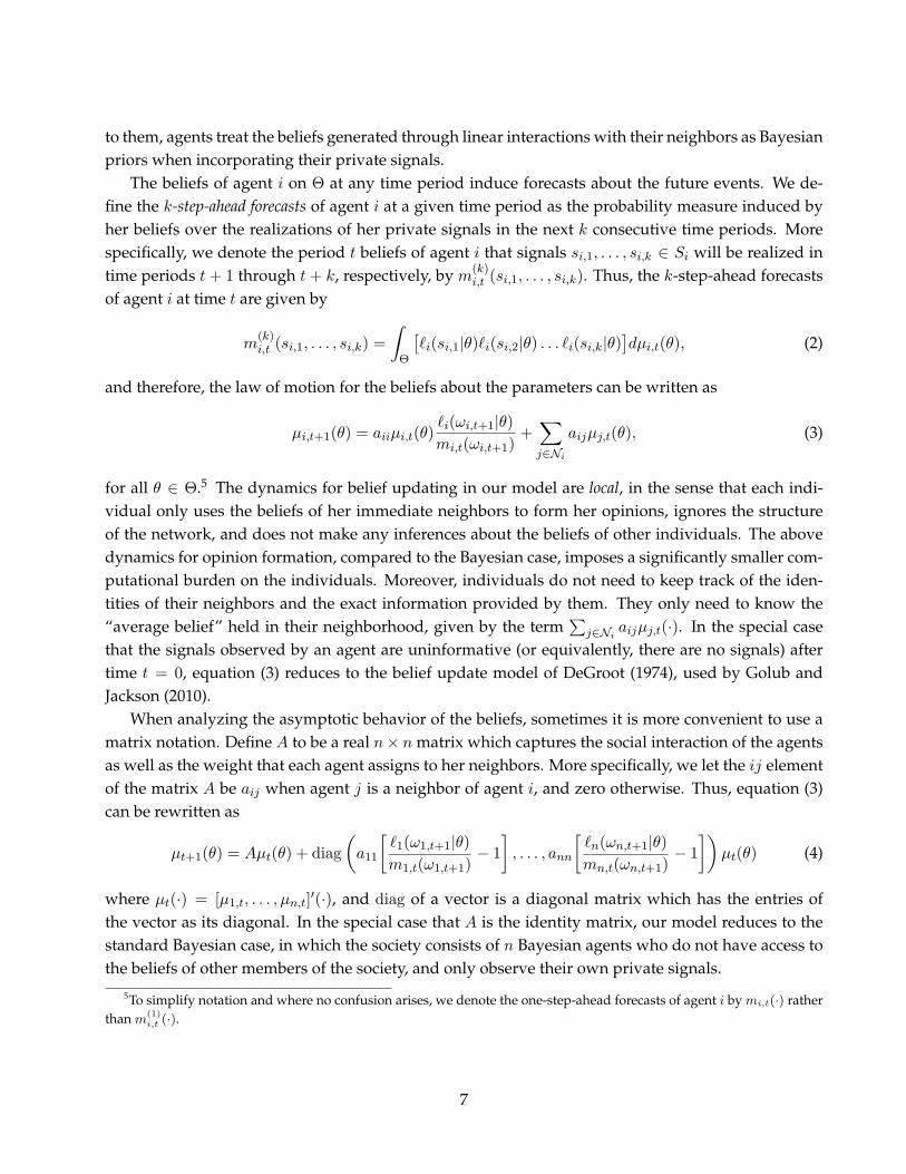
for all θ ∈ Θ.5 The dynamics for belief updating in our model are local, in the sense that each indi-vidual only uses the beliefs of her immediate neighbors to form her opinions, ignores the structureof the network, and does not make any inferences about the beliefs of other individuals. The abovedynamics for opinion formation, compared to the Bayesian case, imposes a significantly smaller com-putational burden on the individuals. Moreover, individuals do not need to keep track of the iden-tities of their neighbors and the exact information provided by them. They only need to know the“average belief” held in their neighborhood, given by the term

∑j∈Ni

aijµj,t(·). In the special casethat the signals observed by an agent are uninformative (or equivalently, there are no signals) aftertime t = 0, equation (3) reduces to the belief update model of DeGroot (1974), used by Golub andJackson (2010).

When analyzing the asymptotic behavior of the beliefs, sometimes it is more convenient to use amatrix notation. Define A to be a real n× n matrix which captures the social interaction of the agentsas well as the weight that each agent assigns to her neighbors. More specifically, we let the ij elementof the matrix A be aij when agent j is a neighbor of agent i, and zero otherwise. Thus, equation (3)can be rewritten as

µt+1(θ) = Aµt(θ) + diag(a11

[`1(ω1,t+1|θ)m1,t(ω1,t+1)

− 1], . . . , ann

[`n(ωn,t+1|θ)mn,t(ωn,t+1)

− 1])

µt(θ) (4)

where µt(·) = [µ1,t, . . . , µn,t]′(·), and diag of a vector is a diagonal matrix which has the entries ofthe vector as its diagonal. In the special case that A is the identity matrix, our model reduces to thestandard Bayesian case, in which the society consists of n Bayesian agents who do not have access tothe beliefs of other members of the society, and only observe their own private signals.

5To simplify notation and where no confusion arises, we denote the one-step-ahead forecasts of agent i by mi,t(·) ratherthan m(1)

i,t (·).

7

4 Social Learning

Given the model described above, we are interested in the evolution of opinions in the network, andwhether this evolution can lead to learning in the long run. Learning may either signify uncoveringthe true parameter or learning to forecast future outcomes. These two notions of learning are distinctand might not occur simultaneously. We start this section by specifying the exact meaning of bothtypes of learning. Recall that θ∗ ∈ Θ is the underlying state of the world and thus, the measureP∗ = ⊗∞t=1`(·|θ∗) is the probability law generating the signals (ω1, ω2, . . . ) ∈ Ω.

Definition 1. The k-step-ahead forecasts of agent i are eventually correct on a path ω = (ω1, ω2, . . . ) if,along that path,

m(k)i,t (si,1, si,2, . . . , si,k) −→ `i(si,1|θ∗)`i(si,2|θ∗) . . . `i(si,k|θ∗) as t→∞

for all (si,1, . . . , si,k) ∈ Ski . Moreover, we say the beliefs of agent i weakly merge to the truth on somepath if, along that path, her k-step-ahead forecasts are eventually correct for all natural numbers k.

This notion of learning, used by Kalai and Lehrer (1994), captures the ability of agents to correctlyforecast events in the near future. It is well-known that, under suitable assumption, repeated appli-cations of Bayes’ rule leads to eventually correct forecasts with probability 1 under the truth. The keycondition is absolute continuity of the true measure with respect to initial beliefs.6 In the presenceof absolute continuity, the mere repetition of Bayes’ rule eventually transforms the historical recordinto a near perfect guide for the future. However, predicting events in near future accurately is notthe same as learning the underlying state of the world. In fact, depending on the signal structure ofeach agent, there might be an “identification problem” which can potentially prevent the agent fromlearning the true parameter θ∗. We define an alternative notion of asymptotic learning where agentsuncover the underlying parameter:

Definition 2. Agent i ∈ N asymptotically learns the true parameter θ∗ on a path ω = (ω1, ω2, . . . ) if,along that path,

µi,t(θ∗) −→ 1 as t→∞.

Asymptotic learning occurs when agent assigns probability one to the true parameter. As men-tioned earlier, making correct forecasts about future events does not necessarily guarantee learningthe true state. In general, the converse is not true either.7 However, it is straightforward to show thatin our model, asymptotically learning θ∗ implies eventually correct forecasts.

4.1 Correct One-Step-Ahead Forecasts

We now turn to the main question of this paper: under what circumstances does learning occur overthe social network?

6Lehrer and Smorodinsky (1996) show that an assumption weaker than absolute continuity, known as accommodation, issufficient for weak merging of the opinion.

7See Lehrer and Smorodinsky (1996), for an example of the case that learning the true parameter does not generallyguarantee weak merging.

8

Our first result shows that under mild assumptions, in spite of local interactions, limited observ-ability, and the non-Bayesian belief update, agents will eventually have correct one-step-ahead fore-casts. The proof is provided in the Appendix.

Proposition 1. Suppose that the social network is strongly connected, all agents have strictly positive self-reliances, and there exists an agent with positive prior belief on the true parameter θ∗. Then, the one-step-aheadforecasts of all agents are eventually correct with P∗-probability one.

This proposition states that, when agents use non-Bayesian updating rule (3) to form and updatetheir opinions, they will eventually make accurate predictions about the realization of their privatesignals in the next period. Note that as long as the social network remains strongly connected, neitherthe topology of the network nor the influence levels of different individuals prevent agents frommaking correct predictions.

One of the features of Proposition 1 is the absence of absolute continuity of the true measure withrespect to the prior beliefs of all agents in the society: as long as some agent assigns a positive priorbelief to the true parameter θ∗ all agents will eventually be able to correctly predict the next periodrealizations of their private signals in the sense of Definition 1. In fact, eventually correct one-step-ahead forecasts arises even if the only agent for whom absolute continuity holds is located at thefringe of the society, has very small persuasive power over her neighbors, and almost everyone in thenetwork is unaware of her existence. The main reason for this phenomenon is that, due to the naıvepart of the updating, there is a “contagion” of beliefs to all agents, which eventually leads to absolutecontinuity of their beliefs with respect to the truth.

Besides the existence of an agent with a positive prior belief on the true state, the above proposi-tion requires the existence of positive self-reliances to guarantee correct forecasts. This requirement isintuitive: it prohibits agents from completely discarding information provided to them through theirobservations. Clearly, if all agents discard their private signals, no new information is incorporatedinto their opinions, and (3) simply turns into a diffusion of prior beliefs.

The final requirement for accurate predictions is strong connectivity of the social network. Thefollowing example illustrates that this assumption cannot be disposed of.

Example 1. Consider a society consisting of two agents, N = 1, 2, and assume that Θ = θ1, θ2with the true state being θ∗ = θ1. Both agents have non-degenerate prior beliefs over Θ. Assumethat signals observed by the agents are conditionally independent, and belong to the set S1 = S2 =H,T. We further assume that Agent 2’s signals are non-informative, while Agent 1’s observationsare perfectly informative about the state; that is, `1(H|θ1) = `1(T |θ2) = 1, and `2(s|θ1) = `2(s|θ2) fors ∈ H,T. As for the social structure, we assume that Agent 1 has access to the opinion of Agent2, while Agent 2 cannot observe the opinion of Agent 1. Clearly, the social network is not stronglyconnected. We let the social interaction matrix be

A =[1− α α

0 1

],

where α ∈ (0, 1) is the weight that Agent 1 assigns to the opinion of Agent 2, when updating herbeliefs using equation (3). Since the private signals observed by the latter are non-informative, her be-

9

liefs, at all times, remain equal to her prior. Clearly, she makes correct forecasts at all times. Agent 1’sforecasts, on the other hand, will always remain incorrect. Notice that since her signals are perfectlyinformative, Agent 1’s one-step-ahead predictions are eventually correct if and only if she eventuallyassigns probability 1 to the true state, θ1. However, the belief she assigns to θ2 follows the law ofmotion

µ1,t+1(θ2) = (1− α)µ1,t(θ2)`1(ω1,t+1|θ2)m1,t(ω1,t+1)

+ αµ2,t(θ2)

which cannot converge to zero, as µ2,t(θ2) = µ2,0(θ2) is strictly positive.The intuition for failure of learning in this example is simple. Given the same observations, the

two agents make different interpretations about the state, even if they have equal prior beliefs. More-over, Agent 1 follows the beliefs of the less informed Agent 2 but is unable to influence her back. Thisone-way persuasion and non-identical interpretations of signals (due to non-identical signal struc-tures) result in incorrect one-step-ahead forecasts on the part of Agent 1. Finally, note that had Agent1 discarded the opinions of Agent 2 and updated her beliefs according to Bayes’ rule, she would havelearned the truth after a single observation.

4.2 Weak Merging to the Truth

The key implication of Proposition 1 is that as long as the social network is strongly connected, theone-step-ahead forecasts of all agents will eventually be correct. Our next result establishes that notonly agents make accurate predictions about their private observations in the next period, but also,under the same set of assumptions, make correct predictions about any finite time horizon in thefuture.

Proposition 2. Suppose that the social network is strongly connected, all agents have strictly positive self-reliances, and there exists an agent with positive prior belief on the true parameter θ∗. Then, the beliefs of allagents weakly merge to the truth with P∗-probability one.

The above proposition states that in strongly connected societies, having eventually correct one-step-ahead forecasts is equivalent to weak merging of agents’ opinions to the truth. This equivalencehas already been established by Kalai and Lehrer (1994) for Bayesian agents. Note that in the purelyBayesian case, an agent’s k-step-ahead forecasts are simply products of her one-step-ahead forecasts,making the equivalence between one-step-ahead correct forecasts and weak merging of opinions im-mediate. However, due to the non-Bayesian updating of the beliefs, the k-step-ahead forecasts ofagents in our model do not have such a multiplicative decomposition, making this implication signif-icantly less straightforward.

4.3 Social Learning

Proposition 2 shows that in strongly connected social networks, the predictions of all individualsabout the realizations of their signals in any finite time horizon will eventually be correct, implyingthat their asymptotic opinions cannot be arbitrary. The following proposition, which is our mainresult, establishes that strong connectivity of the social network not only leads to correct forecasts,

10

but also guarantees successful aggregation of information: all individuals eventually learn the truestate.

Proposition 3. Suppose that:

(a) The social network is strongly connected.

(b) All agents have strictly positive self-reliances.

(c) There exists an agent with positive prior belief on the true parameter θ∗.

(d) There is no state θ 6= θ∗ that is observationally equivalent to θ∗ from the point of view of all agents in thenetwork.

Then, all agents in the social network learn the true state of the world P∗-almost surely; that is, µi,t(θ∗) −→ 1with P∗-probability one for all i ∈ N , as t→∞.

Proposition 3 states that under regularity assumptions on the social network’s topology and theindividuals’ signal structures, all agents will eventually learn the true underlying state of the world.Notice that agents only interact with their neighbors and perform no deductions about the worldbeyond their immediate neighbors. Nonetheless, the non-Bayesian updating rule eventually enablesthem to obtain relevant information from others, without exactly knowing where it comes from. Infact, they can be completely oblivious to important features of the social network — such as thenumber of individuals in the society, the topology of the network, other people’s signal structures,the existence of some agent who considers the truth plausible, or the influence level of any agentin the network — and still learn the true parameter as if they were informed of all observationsand updated their beliefs according to Bayes’ rule. Moreover, all these results are achieved with asignificantly smaller computational burden than what is required for Bayesian learning.

The other significant feature of Proposition 3 is that neither network’s topology, the signal struc-tures, nor the influence levels of different agents prevent learning. For instance, even if the agentswith the least informative signals are the most persuasive ones and are located at the bottlenecks ofthe network, everyone will eventually learn the true state. Social learning is achieved despite the factthat the truth is not recognizable to any individual, and she would not have learned it by herself inisolation.

The intuition behind Proposition 3 is simple. Recall that Proposition 2 implies that the vectorof beliefs of individual i, i.e., µi,t(·), cannot vary arbitrarily forever, and instead, will eventually berestricted to the subspace that guarantees correct forecasts. Asymptotic convergence to such a sub-space requires that she assigns an asymptotic belief of zero to any state θ which is not observationallyequivalent to the truth from her point of view; otherwise, she would not be able to form correct fore-casts about future realizations of her signals. However, due to the non-Bayesian part of the updatecorresponding to the social interactions of agent i with her neighbors, an asymptotic belief of zero ispossible only if all her neighbors also consider θ asymptotically unlikely. This means that the infor-mation available to agent i must be eventually incorporated into every other individuals’ beliefs.

11

The role of assumptions of Proposition 3 can be summarized as follows: the strong connectiv-ity assumption creates the possibility of information flow between any pair of agents in the socialnetwork. The assumption on positive self-reliances guarantees that agents do not discard the infor-mation provided to them through their private observations. The third assumption states that someagent assigns a positive prior belief to the truth. This agent may be at the fringe of the society, mayhave a very small influence on her neighbors, and almost no one may be aware of her existence.Hence, the ultimate source of learning may remain unknown to almost everyone. Clearly, if the priorbeliefs of all agents assigned to the truth is equal to zero, then they will never learn.

The last assumption indicates that the collection of observations of all agents is informative enoughabout the true state; that is, Θ1 ∩ · · · ∩ Θn = θ∗.8 This assumption guarantees that it is possible tolearn the truth if one has access to the observations of all agents. In the absence of this assumption,even highly sophisticated Bayesian agents with access to all relevant information (such as the topol-ogy of the network and the signal structures), would not be able to completely learn the state, due toan identification problem. Finally, note that when agents have identical signal structures (and there-fore, Θi = Θj for all i and j), they do not benefit from the information provided by their neighbors asthey would be able to asymptotically learn just as much through their private observations.

The next examples show the power and limitations of Proposition 3.

Example 2. Consider the collection of agents N = 1, 2, . . . , 7 who are located in a social networkas depicted in Figure 1: at every time period, agent i ≤ 6 can observe the opinion of agent i + 1 andagent 7 has access to the opinion held by agent 1. Clearly, this is a strongly connected social network.

Assume that the set of possible states of the world is given by Θ = θ∗, θ1, θ2, . . . , θ7, where θ∗ isthe true underlying state of the world. We also assume that the signals observed by the agents belong

Figure 1: A strongly connected social network of 7 agents.

8This is a stronger restriction than requiring `(·|θ) 6= `(·|θ∗) for all θ 6= θ∗. See also Example 4.

12

to the set Si = H,T for all i, are conditionally independent, and have conditional distributionsgiven by

`i(H|θ) =

ii+1 if θ = θi

1(i+1)2

otherwise

for all i ∈ N .The signal structures are such that each agent suffers from some identification problem; i.e., the

information in the observations of any agent is not sufficient for learning the true state of the worldin isolation. More precisely, Θi = Θ/θi for all i, which means that from the point of view of agenti, all states except for θi are observationally equivalent to the true state θ∗. Nevertheless, for anygiven state θ 6= θ∗, there exists an agent whose signals are informative enough to distinguish the two;that is, ∩7

i=1Θi = θ∗. Therefore, Proposition 3 implies that as long as one agent assigns a positiveprior belief on the true state θ∗ and all agents have strictly positive self-reliances, then µi,t(θ∗)→ 1, ast → ∞ for all agents i, with P∗-probability one. In other words, all agents will asymptotically learnthe true underlying state of the world. Clearly, if agents discard the information provided to them bytheir neighbors, they have no means of learning the true state.

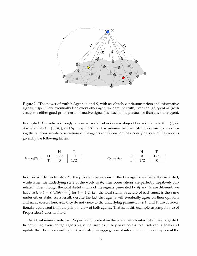
Example 3. Consider a collection of agents who are connected to one another according to the socialnetwork depicted in Figure 2. The values on the edges depict the persuasion power of different agentson each other, where ε > 0 is some arbitrarily small number. As the figure suggests, Agent M is themost influential agent in the network, both in terms of persuasion power and connectivity: she canhighly influence almost everyone in the society, while being only marginally influenced by the publicopinion herself. One can think of M representing a far reaching news media.

Even though highly influential, agent M is not well-informed about the true underlying state ofthe world θ∗ ∈ Θ. More specifically, we assume that her signals are completely non-informative andthat she does not consider θ∗ a possible candidate for the truth, i.e., she assigns a zero prior beliefto that state. In fact, we assume that agent A — who is neither highly persuasive nor can broadcasther opinions beyond her immediate neighbors — is the only agent in the society who assigns somepositive prior belief to θ∗. In addition, we assume that agent S is the only agent in the social networkwith access to informative signals, enabling her to distinguish different states from one another.

Since the social network is strongly connected, Proposition 3 implies that all agents will asymp-totically learn the truth. This is despite the fact that in initial periods, due to the high persuasionpower of agent M and her far reach, the views of all agents (including agents A and S) will move to-wards the initial views of agent M . However, such effects are only transient and will not last forever.As time progresses, due to the possibility of reciprocal persuasion in the network (although highlyasymmetric), the views of agents A and S about the true parameter spread throughout the network.Since such views are consistent with the personal experience of all agents, they are eventually consol-idated all across the social network. Thus, in the tension between high persuasion power and globalreach of M versus the grain of truth of the beliefs and identification ability of the “obscure” agents Aand S, eventually, the latter prevail. These results hold even though at no point in time the truth isrecognizable to any of the agents, including agents A and S themselves.

13

M

A

S

1-

1-

Figure 2: “The power of truth”: Agents A and S, with absolutely continuous priors and informativesignals respectively, eventually lead every other agent to learn the truth, even though agent M (withaccess to neither good priors nor informative signals) is much more persuasive than any other agent.

Example 4. Consider a strongly connected social network consisting of two individuals N = 1, 2.Assume that Θ = θ1, θ2, and S1 = S2 = H,T. Also assume that the distribution function describ-ing the random private observations of the agents conditional on the underlying state of the world isgiven by the following tables:

H T

`(s1s2|θ1) :H 1/2 0T 0 1/2

H T

`(s1s2|θ2) :H 0 1/2T 1/2 0

In other words, under state θ1, the private observations of the two agents are perfectly correlated,while when the underlying state of the world is θ2, their observations are perfectly negatively cor-related. Even though the joint distributions of the signals generated by θ1 and θ2 are different, wehave `i(H|θ1) = `i(H|θ2) = 1

2 for i = 1, 2; i.e., the local signal structure of each agent is the sameunder either state. As a result, despite the fact that agents will eventually agree on their opinionsand make correct forecasts, they do not uncover the underlying parameter, as θ1 and θ2 are observa-tionally equivalent from the point of view of both agents. That is, in this example, assumption (d) ofProposition 3 does not hold.

As a final remark, note that Proposition 3 is silent on the rate at which information is aggregated.In particular, even though agents learn the truth as if they have access to all relevant signals andupdate their beliefs according to Bayes’ rule, this aggregation of information may not happen at the

14

same rate that Bayesian agents would learn. Moreover, the rate of learning may depend on the finedetails of the structure of the social network as well as agents’ signal structures.

5 Conclusions

In this paper, we develop a model of dynamic opinion formation in social networks, bridging the gapbetween the Bayesian and the DeGroot-style non-Bayesian models of social learning. Agents fail toincorporate the views of their neighbors in a fully Bayesian manner, and instead, use a local updatingrule. More specifically, at every time period, the belief of each individual is a convex combinationof her Bayesian posterior belief and her neighbors’ expressed beliefs. Our results show that agentseventually make correct forecasts, as long as the social network is strongly connected. In addition,agents successfully aggregate all information over the entire social network: they eventually learn thetrue underlying state of the world as if they were completely informed of all signals and updated theirbeliefs according to Bayes’ rule.

The main insight suggested by our results is that, with a constant flow of new information, the keycondition for social learning is that individuals take their personal signals into account in a Bayesianway. Repeated interactions over the social network guarantee that the differences of opinions eventu-ally vanish and learning is obtained. The aggregation of information is achieved even if individualsare unaware of important features of the environment. In particular, agents do not need to have anyinformation (or form beliefs) about the structure of the social network nor the views or characteristicsof most agents, as they only update their opinions locally and do not make any deductions about theworld beyond their immediate neighbors. Moreover, the individuals do not need to know the signalstructure of any other agent in the network, besides their own. Thus, individuals eventually achievefull learning through a simple local updating rule and avoid the highly complex computations thatare essential for full Bayesian updating over the network.

Even though our results establish that asymptotic learning is achieved in all strongly connectedsocial networks, the rate at which information is aggregated depends on the topology of the networkas well as agents’ signal structures. Relatedly, the fine details of the social network structure wouldalso affect asymptotic learning if agents’ influences vary over time. In particular, if the influences ofindividuals on their neighbors vanish over time, disagreements may persist even if the social networkis strongly connected. Characterizing the relationship between the structure of the social networkand the rate of learning is an important direction for future research. Another feature of the modelstudied in this paper is the assumption that agents can communicate their beliefs with their neighbors;a potentially unrealistic assumption when the size of the state space is large. This leads to the openquestions of whether there are more efficient modes of communication and whether asymptotic sociallearning can be sustained when agents communicate some sufficient statistics of their beliefs with oneanother. We intend to investigate these questions in future work.

15

Appendix: Proofs

A.1 Two Auxiliary Lemmas

Before presenting the proofs of the results in the paper, we state and prove two lemmas, both of whichare consequences of the martingale convergence theorem.

Lemma 1. Let A denote the matrix of social interactions. The sequence∑n

i=1 viµi,t(θ∗) converges P∗-almost

surely as t→∞, where v is any non-negative left eigenvector of A corresponding to its unit eigenvalue.

Proof: First, note that sinceA is stochastic,9 it always has at least one eigenvalue equal to 1. Moreover,there exists a non-negative left eigenvector corresponding to this eigenvalue.10 We denote such avector by v.

Evaluate equation (4) at the true parameter θ∗ and multiply both sides by v′ from left

v′µt+1(θ∗) = v′Aµt(θ∗) +n∑i=1

viµi,t(θ∗)aii

[`i(ωi,t+1|θ∗)mi,t(ωi,t+1)

− 1].

Thus,

E∗[

n∑i=1

viµi,t+1(θ∗)|Ft

]=

n∑i=1

viµi,t(θ∗) +n∑i=1

viaiiµi,t(θ∗)E∗[`i(ωi,t+1|θ∗)mi,t(ωi,t+1)

− 1|Ft], (5)

where E∗ denotes the expectation operator associated with measure P∗. Since f(x) = 1/x is a convexfunction, Jensen’s inequality implies that

E∗[`i(ωi,t+1|θ∗)mi,t(ωi,t+1)

|Ft]≥(

E∗[mi,t(ωi,t+1)`i(ωi,t+1|θ∗)

|Ft])−1

= 1,

and therefore,

E∗[

n∑i=1

viµi,t+1(θ∗)|Ft

]≥

n∑i=1

viµi,t(θ∗).

The last inequality is due to the fact that v is element-wise non-negative. As a result,∑n

i=1 viµi,t(θ∗)

is a submartingale with respect to the filtration Ft, which is also bounded above by ‖v‖1. Hence, itconverges P∗-almost surely.

Lemma 2. Suppose that there exists an agent i such that µi,0(θ∗) > 0. Also suppose that the social network isstrongly connected. Then, the sequence

∑ni=1 vi logµi,t(θ∗) converges P∗-almost surely as t → ∞, where v is

any non-negative left eigenvector of A corresponding to its unit eigenvalue.

Proof: Similar to the proof of the previous lemma, we show that∑n

i=1 vi logµi,t(θ∗) is a boundedsubmartingale and invoke the martingale convergence theorem to obtain almost sure convergence.

9A matrix is said to be stochastic if it is entry-wise non-negative and all its row sums are equal to one.10This is a consequence of the Perron-Frobenius theorem. For more on the properties of non-negative and stochastic

matrices, see Berman and Plemmons (1979).

16

By evaluating the law of motion at θ∗, taking log from both sides, and using the fact that the rowsums of A are equal to one, we obtain

logµi,t+1(θ∗) ≥ aii logµi,t(θ∗) + aii log(`i(ωi,t+1|θ∗)mi,t(ωi,t+1)

)+∑j∈Ni

aij logµj,t(θ∗),

where we have used the concavity of the logarithm function. Note that since the social network isstrongly connected, the existence of one agent with a positive prior on θ∗ guarantees that after atmost n periods all agents assign a strictly positive probability to the true parameter, which meansthat logµi,t(θ∗) is well-defined for large enough t and all i.

Our next step is to show that E∗[log `i(ωi,t+1|θ∗)

mi,t(ωi,t+1) |Ft]≥ 0. To obtain this,

E∗[log

`i(ωi,t+1|θ∗)mi,t(ωi,t+1)

|Ft]

= −E∗[log

mi,t(ωi,t+1)`i(ωi,t+1|θ∗)

|Ft]

≥ − log(

E∗[mi,t(ωi,t+1)`i(ωi,t+1|θ∗)

|Ft])

= 0.

Thus,E∗ [logµi,t+1(θ∗)|Ft] ≥ aii logµi,t(θ∗) +

∑j∈Ni

aij logµj,t(θ∗),

which can be rewritten in matrix form as E∗ [logµt+1(θ∗)|Ft] ≥ A logµt(θ∗), where by the logarithmof a vector, we mean its entry-wise logarithm. Multiplying both sides by A’s non-negative left eigen-vector v′ leads to

E∗[

n∑i=1

vi logµi,t+1(θ∗)|Ft

]≥

n∑i=1

vi logµi,t(θ∗).

Thus, the non-positive sequence∑n

i=1 vi logµi,t(θ∗) is a submartingale with respect to filtration Ft,and therefore, converges with P∗-probability one.

With these lemmas in hand, we can prove Proposition 1.

A.2 Proof of Proposition 1

First, note that since the social network is strongly connected, the social interaction matrix A is anirreducible stochastic matrix, and therefore its left eigenvector corresponding to the unit eigenvalueis strictly positive.11

According to Lemma 1,∑n

i=1 viµi,t(θ∗) converges with P∗-probability one, where v is the positive

left eigenvector of A corresponding to its unit eigenvalue. Therefore, equation (5) implies that

n∑i=1

viaiiµi,t(θ∗)(

E∗[`i(ωi,t+1|θ∗)mi,t(ωi,t+1)

|Ft]− 1)−→ 0 P∗-a.s.

11An n× n matrix A is said to be reducible, if for some permutation matrix P , the matrix P ′AP is block upper triangular.If a square matrix is not reducible, it is said to be irreducible. For more on this, see e.g., Berman and Plemmons (1979).

17

Since the term viaiiµi,t(θ∗)E∗ [`i(ωi,t+1|θ∗)/mi,t(ωi,t+1)− 1|Ft] is non-negative for all i, each such termconverges to zero with P∗-probability one. Moreover, the assumptions that all diagonal entries of Aare strictly positive and that of its irreducibility (which means that v is entry-wise positive) lead to

µi,t(θ∗)(

E∗[`i(ωi,t+1|θ∗)mi,t(ωi,t+1)

|Ft]− 1)−→ 0 for all i P∗-a.s. (6)

Furthermore, Lemma 2 guarantees that∑n

i=1 vi logµi,t(θ∗) converges almost surely, implying thatµi,t(θ∗) is uniformly bounded away from zero for all i with probability one. Note that, once again

we are using the fact that v is a strictly positive vector. Hence, E∗[`i(ωi,t+1|θ∗)mi,t(ωi,t+1) |Ft

]→ 1 almost surely.

Thus,

E∗[`i(ωi,t+1|θ∗)mi,t(ωi,t+1)

|Ft]− 1 =

∑si∈Si

`i(si|θ∗)(`i(si|θ∗)mi,t(si)

− 1)

=∑si∈Si

(`i(si|θ∗)

`i(si|θ∗)−mi,t(si)mi,t(si)

+mi,t(si)− `i(si|θ∗))

=∑si∈Si

[`i(si|θ∗)−mi,t(si)]2

mi,t(si)−→ 0 P∗-a.s.,

where the second equality is due to the fact that both `i(·|θ∗) and mi,t(·) are probability measures onSi, and therefore,

∑si∈Si

`i(si|θ∗) =∑

si∈Simi,t(si) = 1.

In the last expression, the term in the braces and the denominator are always non-negative andtherefore,

mi,t(si) −→ `i(si|θ∗) P∗-a.s.

for all si ∈ Si and all i ∈ N .

A.3 Proof of Proposition 2

We first present and prove a simple lemma which is later used in the proof of the proposition.

Lemma 3. Suppose that the social network is strongly connected, all agents have strictly positive self-reliances,and there exists an agent i such that µi,t(θ∗) > 0. Then, for all θ ∈ Θ,

E∗ [µt+1(θ)|Ft]−Aµt(θ) −→ 0

with P∗-probability one, as t→∞.

Proof: Taking conditional expectations from both sides of equation (4) implies

E∗ [µt+1(θ)|Ft]−Aµt(θ) = diag(a11E∗

[`1(ω1,t+1|θ)m1,t(ω1,t+1)

− 1|Ft], . . . , annE∗

[`n(ωn,t+1|θ)mn,t(ωn,t+1)

− 1|Ft])

µt(θ).

On the other hand, we have

E∗[`i(ωi,t+1|θ)mi,t(ωi,t+1)

|Ft]

=∑si∈Si

`i(si|θ)`i(si|θ∗)mi,t(si)

−→∑si∈Si

`i(si|θ) P∗-a.s.

18

where the convergence is a consequence of Proposition 1. The fact that `i(·|θ) is a probability measureon Si implies

∑si∈Si

`i(si|θ) = 1, completing the proof.

We now present the proof of Proposition 2.

Proof of Proposition 2:12 We prove this proposition by induction. Note that by definition, agent i’sbeliefs weakly merge to the truth if her k-step-ahead forecasts are eventually correct for all naturalnumbers k. In Proposition 1, we established that the claim is true for k = 1. For the rest of the proof,we assume that the claim is true for k−1 and show thatm(k)

i,t (si,1, . . . , si,k) converges to∏kr=1 `i(si,r|θ∗)

for any arbitrary sequence of signals (si,1, . . . , si,k) ∈ Ski .First, note that Lemma 3 and equation (3) imply that for all θ ∈ Θ,

E∗[µi,t+1(θ)|Ft]− µi,t+1(θ) + aii

[`i(ωi,t+1|θ)mi,t(ωi,t+1)

− 1]µi,t(θ) −→ 0 P∗-a.s.

On the other hand, we have

∑θ∈Θ

(k∏r=2

`i(si,r|θ)

)(E∗[µi,t+1(θ)|Ft]− µi,t+1(θ)

)= E∗

[m

(k−1)i,t+1 (si,2, . . . , si,k)|Ft

]−m(k−1)

i,t+1 (si,2, . . . , si,k)

→ 0 P∗-a.s.

where we have used the induction hypothesis and the dominated convergence theorem for condi-tional expectations.13 Combining the two equations above implies

∑θ∈Θ

(k∏r=2

`i(si,r|θ)

)[`i(ωi,t+1|θ)mi,t(ωi,t+1)

− 1]µi,t(θ) −→ 0 P∗-a.s.

which can be rewritten as

1mi,t(ωi,t+1)

m(k)i,t (ωi,t+1, si,2, . . . , si,k)−m

(k−1)i,t (si,2, . . . , si,k) −→ 0

with P∗-probability one. Thus, by the induction hypothesis,

m(k)i,t (ωi,t+1, si,2, . . . , si,k)−mi,t(ωi,t+1)

k∏r=2

`i(si,r|θ∗) −→ 0

with P∗-probability one. The dominated convergence theorem for conditional expectations impliesthat

E∗[∣∣∣∣m(k)

i,t (ωi,t+1, si,2, . . . , si,k)−mi,t(ωi,t+1)k∏r=2

`i(si,r|θ∗)∣∣∣∣|Ft

]−→ 0 P∗-a.s.

12We would like to thank an anonymous referee for bringing a technical mistake in an earlier draft of the paper to ourattention.

13For the statement and a proof of the theorem, see page 262 of Durrett (2005).

19

which can be rewritten as∑si∈Si

`i(si|θ∗)∣∣∣∣m(k)

i,t (si, si,2, . . . , si,k)−mi,t(si)k∏r=2

`i(si,r|θ∗)∣∣∣∣ −→ 0

P∗-almost surely, and therefore, guaranteeing

m(k)i,t (si,1, si,2, . . . , si,k)−mi,t(si,1)

k∏r=2

`i(si,r|θ∗) −→ 0 P∗-a.s.

Finally, the fact that mi,t(si,1) −→ `i(si,1|θ∗) with P∗-probability one (Proposition 1) completes theproof.

A.4 Proof of Proposition 3

We first show that for any agent i, there exists a finite sequence of private signals that is more likely torealize under the true state θ∗ than any other state θ, unless θ is observationally equivalent to θ∗ fromthe point of view of agent i.

Lemma 4. For any agent i, there exists a positive integer ki, a sequence of signals (si,1, . . . , si,ki) ∈ (Si)ki ,

and constant δi ∈ (0, 1) such that

ki∏r=1

`i(si,r|θ)`i(si,r|θ∗)

≤ δi ∀θ 6∈ Θi (7)

where Θi = θ ∈ Θ : `i(si|θ) = `i(si|θ∗) for all si ∈ Si.

Proof: By definition, for any θ 6∈ Θi, the probability measures `i(·|θ) and `i(·|θ∗) are distinct. There-fore, by the Kullback-Leibler inequality, there exists some constant εi > 0 such that∑

si∈Si

`i(si|θ∗) log[`i(si|θ∗)`i(si|θ)

]> εi,

for all θ 6∈ Θi, which then implies ∏si∈Si

[`i(si|θ)`i(si|θ∗)

]`i(si|θ∗)< δ′i.

for δ′i = exp(−εi). On the other hand, given the fact that rational numbers are dense on the realline, there exist strictly positive rational numbers q(si)si∈Si — with q(si) chosen arbitrarily close to`i(si|θ∗) — satisfying

∑si∈Si

q(si) = 1, such that14

∏si∈Si

[`i(si|θ)`i(si|θ∗)

]q(si)

< δ′i ∀θ 6∈ Θi. (8)

14The fact that the rationals form a dense subset of the reals means that there are rational numbers q′(si)si∈Si arbitrarilyclose to `i(si|θ∗)si∈Si . Setting q(si) = q′(si)/

Psi∈Si

q′(si) guarantees that one can always find strictly positive rationalnumbers q(si)si∈Si adding up to one, while at the same time, (8) is satisfied.

20

Therefore, the above inequality can be rewritten as

∏si∈Si

[`i(si|θ)`i(si|θ∗)

]k(si)

< (δ′i)ki ∀θ 6∈ Θi

for some positive integers k(si) and ki, satisfying ki =∑

si∈Sik(si). Picking the sequence of signals of

length ki, (si,1, . . . , si,ki), such that si appears k(si) many times in the sequence and setting δi = (δ′i)

ki

proves the lemma.

The above lemma shows that the sequence of private signals in which any signal si ∈ Si appearswith a frequency close enough to `i(si|θ∗) is more likely under the truth θ∗ than any other state θwhich is distinguishable from θ∗. We now proceed to the proof of Proposition 3.

Proof of the Proposition 3: First, we prove that agent i assigns an asymptotic belief of zero on statesthat are not observationally equivalent to θ∗ from her point of view.

Recall that according to Proposition 2, the k-step-ahead forecasts of agent i are eventually correctfor all positive integers k, guaranteeing thatm(k)

i,t (si,1, . . . , si,k) −→∏kr=1 `i(si,k|θ∗) with P∗-probability

one for any sequence of signals (si,1, . . . , si,k). In particular, the claim is true for the integer ki and thesequence of signals (si,1, . . . , si,ki

) satisfying (7) in Lemma 4:

∑θ∈Θ

µi,t(θ)ki∏r=1

`i(si,r|θ)`i(si,r|θ∗)

−→ 1 P∗-a.s.

Therefore, ∑θ 6∈Θi

µi,t(θ)ki∏r=1

`i(si,r|θ)`i(si,r|θ∗)

+∑θ∈Θi

µi,t(θ)− 1 −→ 0 P∗-a.s.

leading to ∑θ 6∈Θi

µi,t(θ)

1−ki∏r=1

`i(si,r|θ)`i(si,r|θ∗)

−→ 0

with P∗-probability one. The fact that ki and (si,1, . . . , si,ki) were chosen to satisfy (7) implies that

1−ki∏r=1

`i(si,r|θ)`i(si,r|θ∗)

> 1− δi > 0 ∀θ 6∈ Θi,

and as a consequence, it must be the case that µi,t(θ)→ 0 as t→∞ for any θ 6∈ Θi. Therefore, with P∗-probability one, agent i assigns an asymptotic belief of zero on any state θ that is not observationallyequivalent to θ∗ from her point of view.

Now consider the belief update rule for agent i given by equation (3), evaluated at some stateθ 6∈ Θi:

µi,t+1(θ) = aiiµi,t(θ)`i(ωi,t+1|θ)mi,t(ωi,t+1)

+∑j∈Ni

aijµj,t(θ).

21

We have already shown that µi,t(θ) −→ 0, P∗-almost surely. However, this is not possible unless∑j∈Ni

aijµj,t(θ) converges to zero as well, which implies that µj,t(θ)→ 0 with P∗-probability one forall j ∈ Ni. Note that this happens even if θ is observationally equivalent to θ∗ from the point of viewof agent j; that is, even if θ ∈ Θj . As a result, all neighbors of agent i will assign an asymptotic beliefof zero to parameter θ regardless of their signal structure. We can extend the same argument to theneighbors of neighbors of agent i, and by induction — since the social network is strongly connected— to all agents in the network. Thus, with P∗-probability one,

µi,t(θ) −→ 0 ∀i ∈ N , ∀θ 6∈ Θ1 ∩ · · · ∩ Θn.

implying that all agents assign an asymptotic belief of zero on states that are not observationallyequivalent to θ∗ from the point of view of all individuals in the society. Therefore, statement (d) in theassumptions of Proposition 3 implies that µi,t(θ) → 0 for all θ 6= θ∗, with P∗-probability one, guaran-teeing complete learning by all agents.

22

References

Acemoglu, Daron, Munther Dahleh, Ilan Lobel, and Asuman Ozdaglar (Forthcoming), “Bayesianlearning in social networks.” The Review of Economic Studies.

Acemoglu, Daron, Asuman Ozdaglar, and Ali Parandeh-Gheibi (2010), “Spread of (mis)informationin social networks.” Games and Economic Behavior, 70, 194 – 227.

Bala, Venkatesh and Sanjeev Goyal (1998), “Learning from neighbors.” The Review of Economic Studies,65, 595–621.

Bala, Venkatesh and Sanjeev Goyal (2001), “Conformism and diversity under social learning.” Eco-nomic Theory, 17, 101–120.

Banerjee, Abhijit (1992), “A simple model of herd behavior.” The Quarterly Journal of Economics, 107,797–817.

Banerjee, Abhijit and Drew Fudenberg (2004), “Word-of-mouth learning.” Games and Economic Behav-ior, 46, 1–22.

Berman, Abraham and Robert J. Plemmons (1979), Nonnegative matrices in the mathematical sciences.Academic Press, New York.

Bikchandani, Sushil, David Hirshleifer, and Ivo Welch (1992), “A theory of fads, fashion, custom, andcultural change as information cascades.” Journal of Political Economy, 100, 992–1026.

DeGroot, Morris H. (1974), “Reaching a consensus.” Journal of American Statistical Association, 69, 118–121.

DeMarzo, Peter M., Dimitri Vayanos, and Jeffery Zwiebel (2003), “Persuasion bias, social influence,and unidimensional opinions.” The Quarterly Journal of Economics, 118, 909–968.

Durrett, Rick (2005), Probability: Theory and Examples, third edition. Duxbury Press, Belmont, CA.

Ellison, Glenn and Drew Fudenberg (1993), “Rules of thumb for social learning.” The Journal of PoliticalEconomy, 101, 612–643.

Ellison, Glenn and Drew Fudenberg (1995), “Word-of-mouth communication and social learning.”The Quarterly Journal of Economics, 110, 93–126.

Epstein, Larry G., Jawwad Noor, and Alvaro Sandroni (2008), “Non-Bayesian updating: a theoreticalframework.” Theoretical Economics, 3, 193–229.

Epstein, Larry G., Jawwad Noor, and Alvaro Sandroni (2010), “Non-Bayesian learning.” The B.E.Journal of Theoretical Economics, 10.

Gale, Douglas and Shachar Kariv (2003), “Bayesian learning in social networks.” Games and EconomicBehavior, 45, 329–346.

23

Golub, Benjamin and Mathew O. Jackson (2010), “Naıve learning in social networks and the wisdomof crowds.” American Economic Journal: Microeconomics, 2, 112–149.

Hagerstrand, Torsten (1969), Innovation Diffusion as a Spatial Process. University of Chicago Press,Chicago, IL.

Kalai, Ehud and Ehud Lehrer (1994), “Weak and strong merging of opinions.” Journal of MathematicalEconomics, 23, 73–86.

Kotler, Philip (1986), The Principles of Marketing, Third edition. Prentice-Hall, New York, NY.

Lehrer, Ehud and Rann Smorodinsky (1996), “Merging and learning.” Statistics, Probability and GameTheory, 30, 147–168.

Mossel, Elchanan and Omer Tamuz (2010), “Efficient Bayesian learning in social networks withGaussian estimators.” Arxiv Preprint arXiv:1002.0747.

Rogers, Everett M. (1983), Diffusion of Innovations, Third edition. Free Press, New York.

Smith, Lones and Peter Norman Sørensen (2000), “Pathological outcomes of observational learning.”Econometrica, 68, 371–398.

24