www.dewesoft.com - Copyright © 2000 - 2020 Dewesoft d.o.o., all rights reserved.

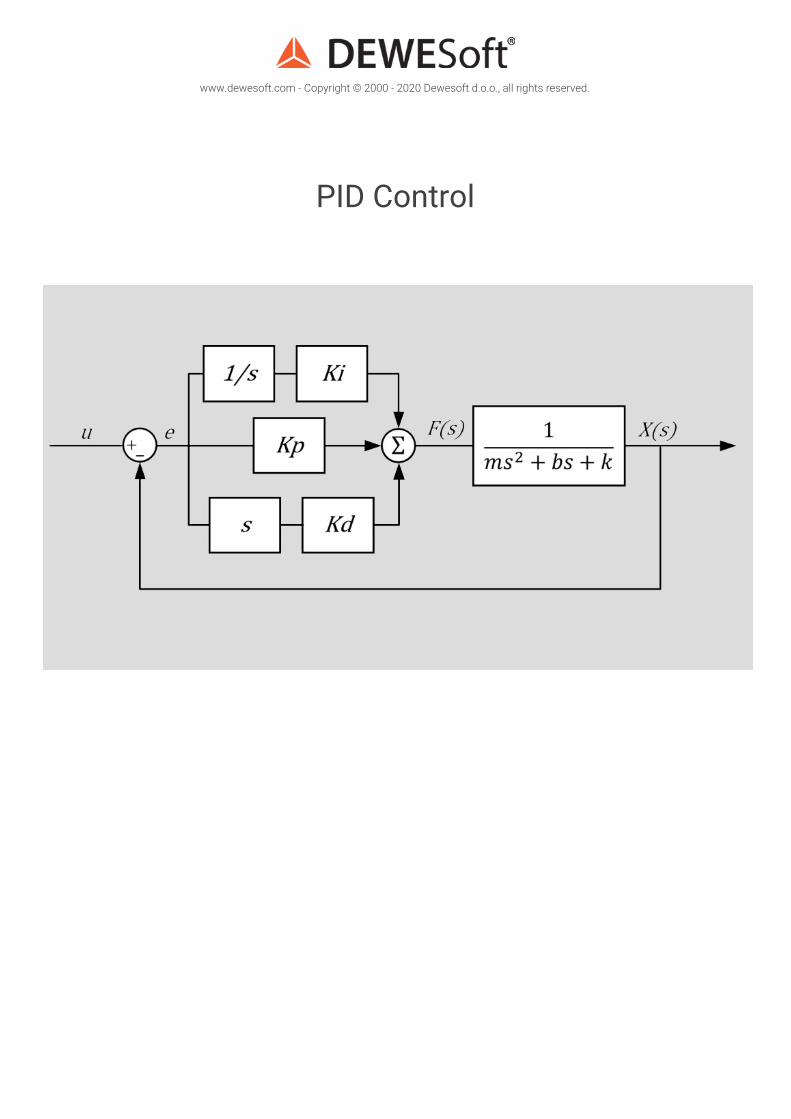
PID Control

Introduction to process controlA controller is a mechanism that controls the output of a system by adjusting its control input. A feedback controllercontinuously measures the output, compares it to the desired output (the set point) and adjusts the input depending on thecalculated error. A PID controller is the most common type of a feedback controller. It adjusts the control variable dependingon the present error (P - proportional control), the accumulated error in the past (I - integral control) and the predicted futureerror (D - derivative control).

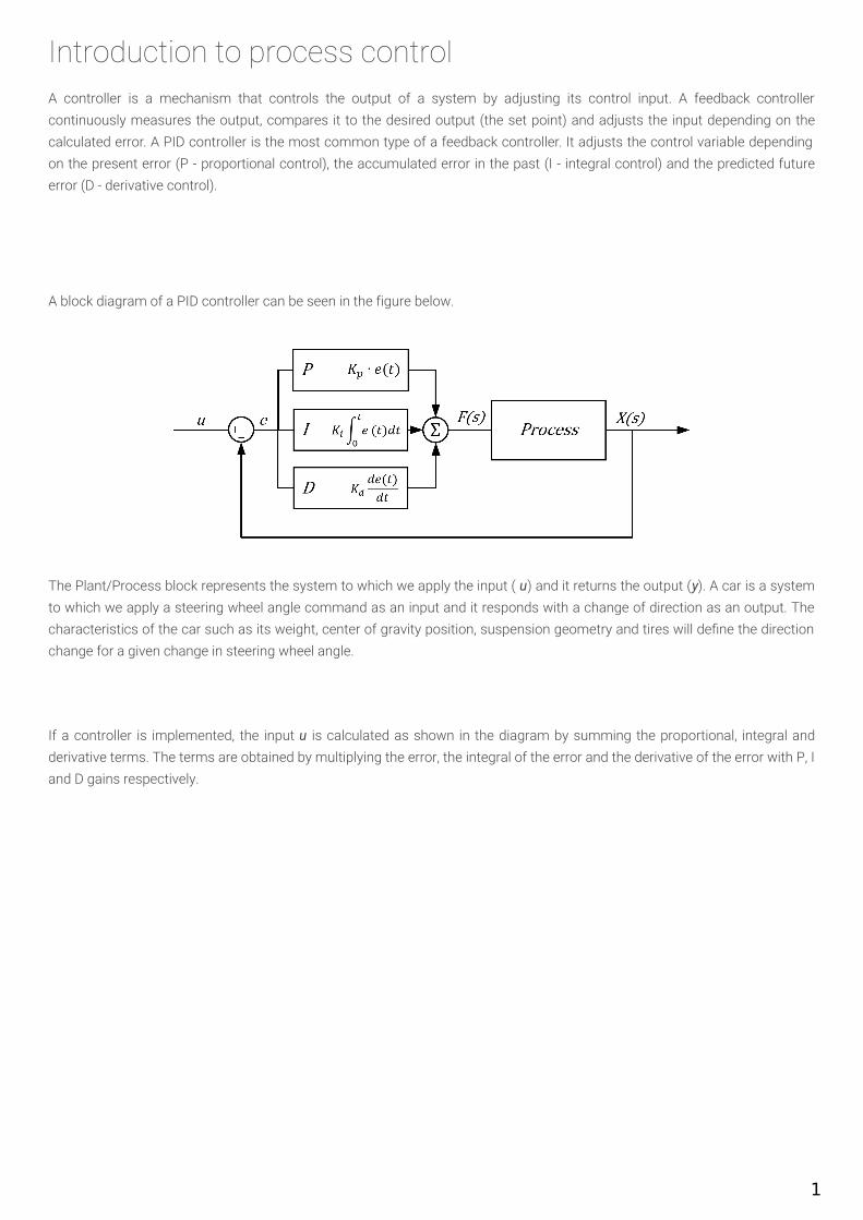
A block diagram of a PID controller can be seen in the figure below.

The Plant/Process block represents the system to which we apply the input ( u) and it returns the output (y). A car is a systemto which we apply a steering wheel angle command as an input and it responds with a change of direction as an output. Thecharacteristics of the car such as its weight, center of gravity position, suspension geometry and tires will de ne the directionchange for a given change in steering wheel angle.

If a controller is implemented, the input u is calculated as shown in the diagram by summing the proportional, integral andderivative terms. The terms are obtained by multiplying the error, the integral of the error and the derivative of the error with P, Iand D gains respectively.

1

The role of the controller gains (Kp, Kd, Ki)Let's look at an example to get a better feeling for the practical implementation of a PID controller. Figure 2 shows a spring-mass-damper system. We will only consider the horizontal motion of the mass. We would like to apply a force f(t) thatdisplaces the mass m to the distance x0 from the initial position in the shortest possible time.

The equation of motion for the system can be written as follows:

$$m\ddot{x}+b\dot{x}+kx=f(t)$$

For further analysis we will assume the following values for the system constants: m = 2 kg, b = 20 N s/m, k = 10 N/m. Theresponse of the system can be calculated by solving the differential equation. To calculate the response to a step input it ismost convenient to apply the Laplace transform, calculate the step response in the frequency domain and then apply theinverse of a Laplace transform to get the response in time domain.

In case of an open loop case there is no feedback. The unit force is applied and the system responds as shown in the gurebelow. The steady state amplitude is only at 10% of the desired value and the response is relatively slow. However, open loopanalysis is very useful for analysing the basic system characteristics that help us design the PID controller as we will see later.

Open loop block diagram:

Open loop transfer function:

$$ \frac{X(s)}{F(s)} = \frac{1}{ms^2 + bs + k} $$

2

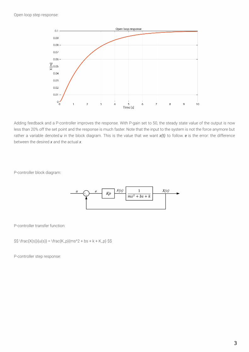
Open loop step response:

Adding feedback and a P-controller improves the response. With P-gain set to 50, the steady state value of the output is nowless than 20% off the set point and the response is much faster. Note that the input to the system is not the force anymore butrather a variable denoted u in the block diagram. This is the value that we want x(t) to follow. e is the error: the differencebetween the desired x and the actual x.

P-controller block diagram:

P-controller transfer function:

$$ \frac{X(s)}{u(s)} = \frac{K_p}{ms^2 + bs + k + K_p} $$

P-controller step response:

3

To get rid of the steady state error we add the I-gain to the controller. In the gure below you can see that the steady stateerror is reduced to zero, but the system first overshoots the set point and then takes longer to settle at the steady state value.

PI-controller block diagram:

PI-controller transfer function:

$$ \frac{X(s)}{u(s)} = \frac{sK_p + K_i}{ms^3 + bs^2 + (k + K_p)s + K_i} $$

PI-controller step response:

4

To get the feeling for what the D-gain does, consider the following case. We would like to shorten the response time of the PIcontroller by increasing the P-gain. The next figure shows the result if the P-gain is increased to 400.

The response is indeed faster but the output oscillates about the set point value. If we increased the P-gain even further, thesystem would become unstable and the output would oscillate with increasing amplitude. The D-gain adds stability to thesystem since it is proportional to the derivative of the error: the faster the error is decreasing, the more negative is thecontribution of the D-term in the equation, decreasing the controller output. By adding the D-gain to our controller and alsotuning the other two gains, the response is fast, with little overshoot and no steady state error.

PID-controller block diagram:

5

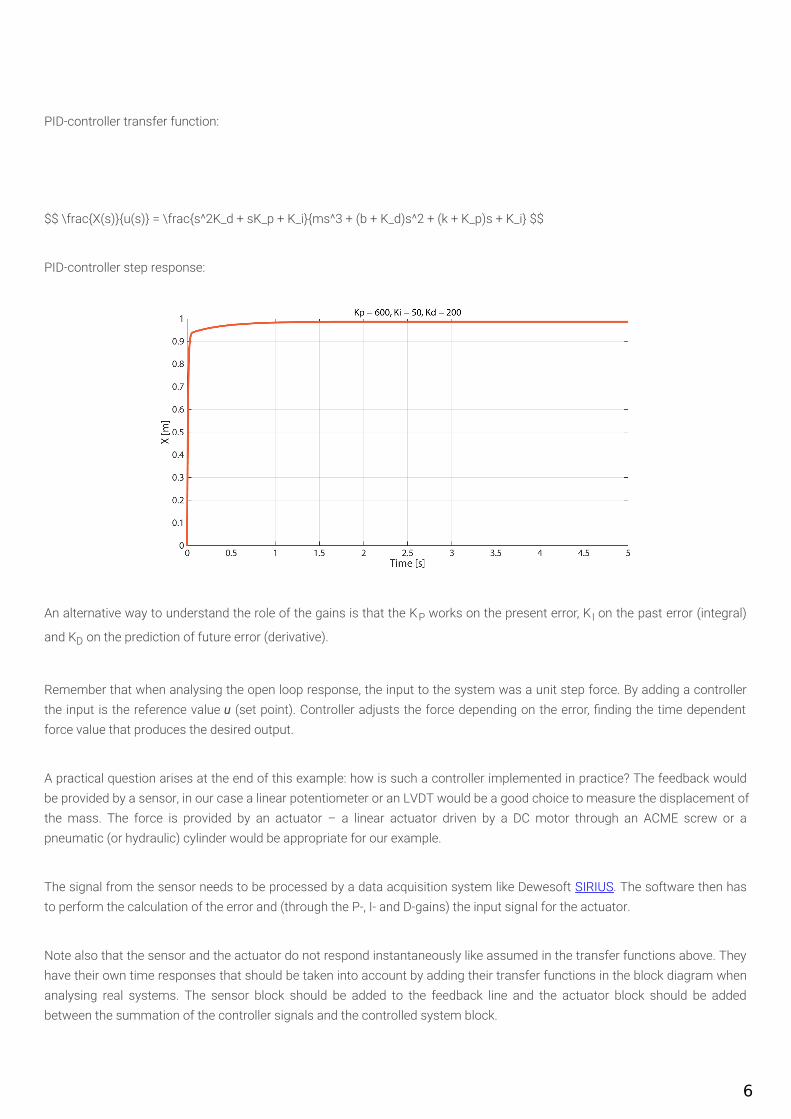
PID-controller transfer function:

$$ \frac{X(s)}{u(s)} = \frac{s^2K_d + sK_p + K_i}{ms^3 + (b + K_d)s^2 + (k + K_p)s + K_i} $$

PID-controller step response:

An alternative way to understand the role of the gains is that the KP works on the present error, K I on the past error (integral)

and KD on the prediction of future error (derivative).

Remember that when analysing the open loop response, the input to the system was a unit step force. By adding a controllerthe input is the reference value u (set point). Controller adjusts the force depending on the error, nding the time dependentforce value that produces the desired output.

A practical question arises at the end of this example: how is such a controller implemented in practice? The feedback wouldbe provided by a sensor, in our case a linear potentiometer or an LVDT would be a good choice to measure the displacement ofthe mass. The force is provided by an actuator – a linear actuator driven by a DC motor through an ACME screw or apneumatic (or hydraulic) cylinder would be appropriate for our example.

The signal from the sensor needs to be processed by a data acquisition system like Dewesoft SIRIUS. The software then hasto perform the calculation of the error and (through the P-, I- and D-gains) the input signal for the actuator.

Note also that the sensor and the actuator do not respond instantaneously like assumed in the transfer functions above. Theyhave their own time responses that should be taken into account by adding their transfer functions in the block diagram whenanalysing real systems. The sensor block should be added to the feedback line and the actuator block should be addedbetween the summation of the controller signals and the controlled system block.

6

The order of the systemBefore designing the PID controller it is useful to identify the order of the system. The system that was analysed in the above

example is a second order system which is evident from its transfer function that has a form of 1/(as 2 + bs + c). We can

recognize a second order system by the s2 in the denominator which is a consequence of a second derivative in the differentialequation.

Another characteristic of the second order system is its open loop step response which can have oscillations about the setpoint. Because of the combination of the m, b and k parameters in the example, the system was overdamped and therefore didnot oscillate. However, if we change the damping parameter b to 2, the step response is underdamped:

A second order system equation can also be rewritten in the following form:

$$ \frac{X(s)}{u(s)} = \frac{K \omega_n^2}{s^2 + 2\xi \omega_n s + \omega_n^2} $$

The constant in the numerator does not change the shape of the response but acts purely as a scaling factor. The values inthe denominator tell us much more about the system. ω n is the natural frequency of the system, which in our example is \(

\sqrt{\frac{k}{m}} \). Parameter ξ is the damping ratio and is equal to \( \frac{b}{2m\omega_n} \) in our example. If we removethe damper from our system (b = 0), the ξ is zero and there is no damping in the system. If ξ = 1 , the system is criticallydamped – this gives the fastest response without oscillations. If ξ > 1, the system is overdamped and if ξ < 1, the system isunderdamped which gives an oscillatory response. Therefore the response of the moving mass in our example can bereasonably tuned by setting the spring and the damper to appropriate values, which is an example of open loop control. Inmany cases the stiffness and damping in the system cannot be tuned directly and closed loop control is needed.

Second order system examplesA displacement response of a spring-mass-damper system to the force input is a typical second order system – the forceon the mass is proportional to the acceleration of the mass, which is the second derivative of the displacement. Anotherexample of a second order system is a voltage response across the capacitor in an RLC circuit to the supply voltage input

7

– voltage across the inductor is proportional to the second derivative of the voltage across the capacitor.

A simpler system is a first order system which has a transfer function of the following form:$$ \frac{X(s)}{u(s)} = \frac{a}{s+a}$$

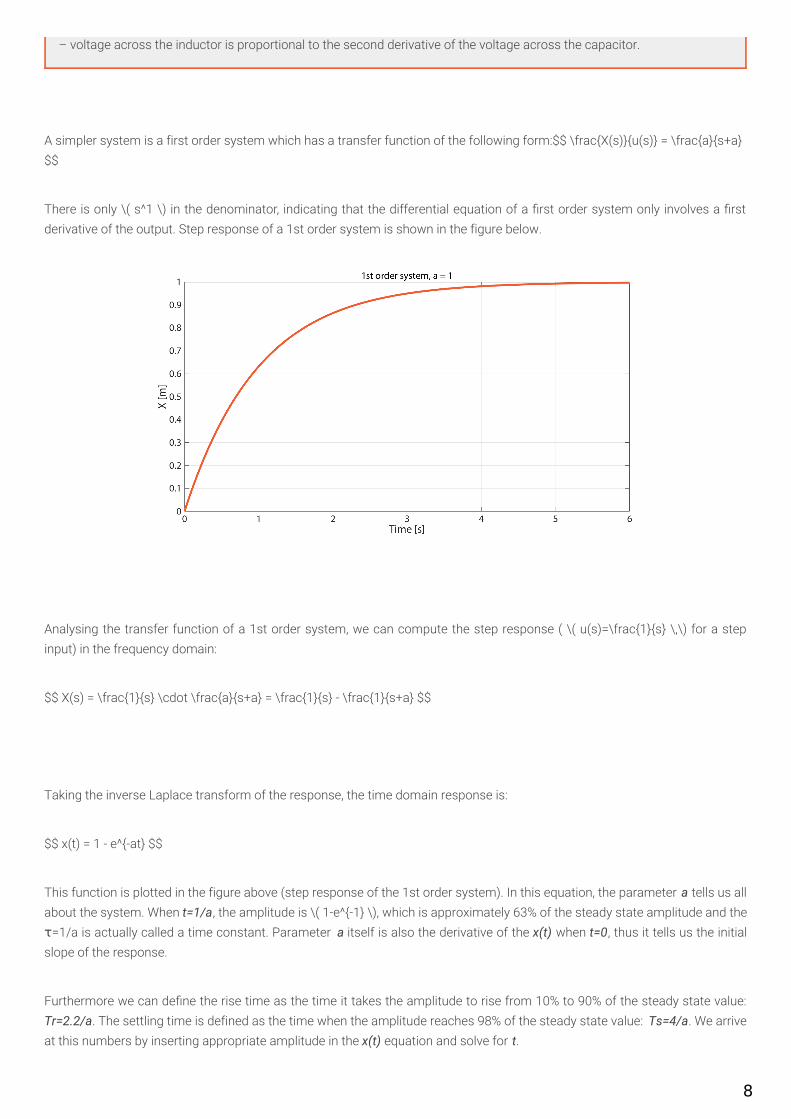
There is only \( s^1 \) in the denominator, indicating that the differential equation of a rst order system only involves a rstderivative of the output. Step response of a 1st order system is shown in the figure below.

Analysing the transfer function of a 1st order system, we can compute the step response ( \( u(s)=\frac{1}{s} \,\) for a stepinput) in the frequency domain:

$$ X(s) = \frac{1}{s} \cdot \frac{a}{s+a} = \frac{1}{s} - \frac{1}{s+a} $$

Taking the inverse Laplace transform of the response, the time domain response is:

$$ x(t) = 1 - e^{-at} $$

This function is plotted in the figure above (step response of the 1st order system). In this equation, the parameter a tells us allabout the system. When t=1/a, the amplitude is \( 1-e^{-1} \), which is approximately 63% of the steady state amplitude and theτ=1/a is actually called a time constant. Parameter a itself is also the derivative of the x(t) when t=0, thus it tells us the initialslope of the response.

Furthermore we can de ne the rise time as the time it takes the amplitude to rise from 10% to 90% of the steady state value:Tr=2.2/a. The settling time is defined as the time when the amplitude reaches 98% of the steady state value: Ts=4/a. We arriveat this numbers by inserting appropriate amplitude in the x(t) equation and solve for t.

8

A more general 1st order system has the transfer function of the following form:

$$ \frac{X(s)}{u(s)} = \frac{k}{s+a} $$

The only difference in the step response is that the amplitude is not 1 but rather k/a, since the time domain response is:

$$ x(t) = \frac{k}{a} \, (1 - e^{-at}) $$

s+a term in the denominator is also called a lag term, because it introduces lag to the system (process variable lags behind thecontrol input).

First order system examplesAn exemplary rst order system is a rotational velocity response of a DC motor to the step voltage input. We metionedthat an RLC circuit has a 2nd order system characteristics. On the other hand, the LR and RC circuits are 1st ordersystems because the supply voltage is related to the voltage or the derivative of the voltage across the respectiveelements in the circuit. Another example is the emptying of the water tank with a valve at the bottom. The pressure at thevalve will decrease exponentially as the water level drops.

9

PID control in Dewesoft XDewesoft X can be used as a PID controller by making use of the PID Control function in the Math section.

WARNING: Dewesoft X software running on Windows is not a real-time system because Windows is not a real-timeoperating system. This means that the delay of the controller is not always the same and can be unpredictable. Forexample Windows could give priority to another application instead of Dewesoft X, which can dramatically increasecontroller delay.

However, a lot of applications do not require real-time control. The controller response time depends on the computerspecifications, but as we will see in the example, the response time can be very short.

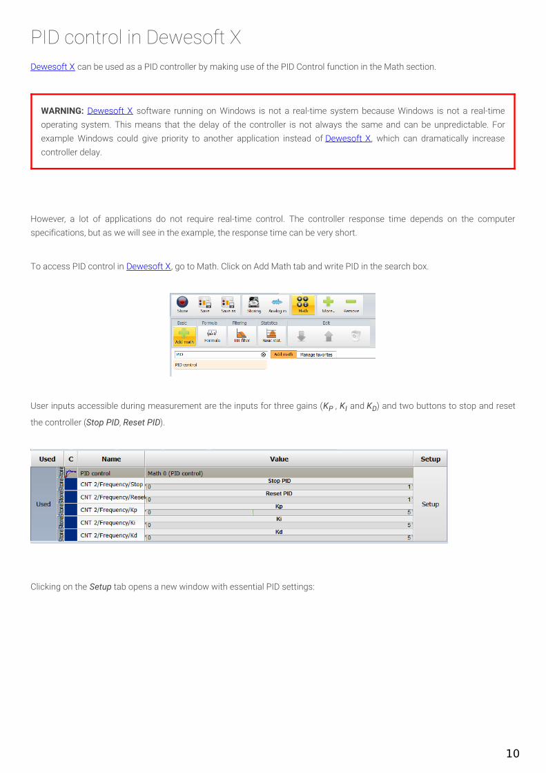
To access PID control in Dewesoft X, go to Math. Click on Add Math tab and write PID in the search box.

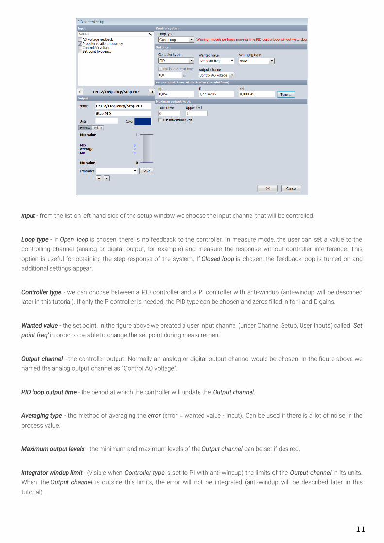
User inputs accessible during measurement are the inputs for three gains (KP , KI and KD) and two buttons to stop and reset

the controller (Stop PID, Reset PID).

Clicking on the Setup tab opens a new window with essential PID settings:

10

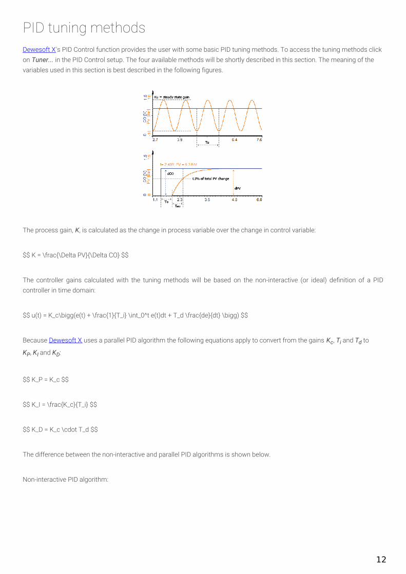
InputInput - from the list on left hand side of the setup window we choose the input channel that will be controlled.

Loop typeLoop type - if Open loop is chosen, there is no feedback to the controller. In measure mode, the user can set a value to thecontrolling channel (analog or digital output, for example) and measure the response without controller interference. Thisoption is useful for obtaining the step response of the system. If Closed loop is chosen, the feedback loop is turned on andadditional settings appear.

Controller typeController type - we can choose between a PID controller and a PI controller with anti-windup (anti-windup will be describedlater in this tutorial). If only the P controller is needed, the PID type can be chosen and zeros filled in for I and D gains.

Wanted valueWanted value - the set point. In the figure above we created a user input channel (under Channel Setup, User Inputs) called 'Setpoint freq' in order to be able to change the set point during measurement.

Output channelOutput channel - the controller output. Normally an analog or digital output channel would be chosen. In the gure above wenamed the analog output channel as "Control AO voltage".

PID loop output timePID loop output time - the period at which the controller will update the Output channel.

Averaging typeAveraging type - the method of averaging the error (error = wanted value - input). Can be used if there is a lot of noise in theprocess value.

Maximum output levelsMaximum output levels - the minimum and maximum levels of the Output channel can be set if desired.

Integrator windup limitIntegrator windup limit - (visible when Controller type is set to PI with anti-windup) the limits of the Output channel in its units.When the Output channel is outside this limits, the error will not be integrated (anti-windup will be described later in thistutorial).

11

PID tuning methodsDewesoft X's PID Control function provides the user with some basic PID tuning methods. To access the tuning methods clickon Tuner... in the PID Control setup. The four available methods will be shortly described in this section. The meaning of thevariables used in this section is best described in the following figures.

The process gain, K, is calculated as the change in process variable over the change in control variable:

$$ K = \frac{\Delta PV}{\Delta CO} $$

The controller gains calculated with the tuning methods will be based on the non-interactive (or ideal) de nition of a PIDcontroller in time domain:

$$ u(t) = K_c\bigg(e(t) + \frac{1}{T_i} \int_0^t e(t)dt + T_d \frac{de}{dt} \bigg) $$

Because Dewesoft X uses a parallel PID algorithm the following equations apply to convert from the gains Kc, Ti and Td to

KP, KI and KD:

$$ K_P = K_c $$

$$ K_I = \frac{K_c}{T_i} $$

$$ K_D = K_c \cdot T_d $$

The difference between the non-interactive and parallel PID algorithms is shown below.

Non-interactive PID algorithm:

12

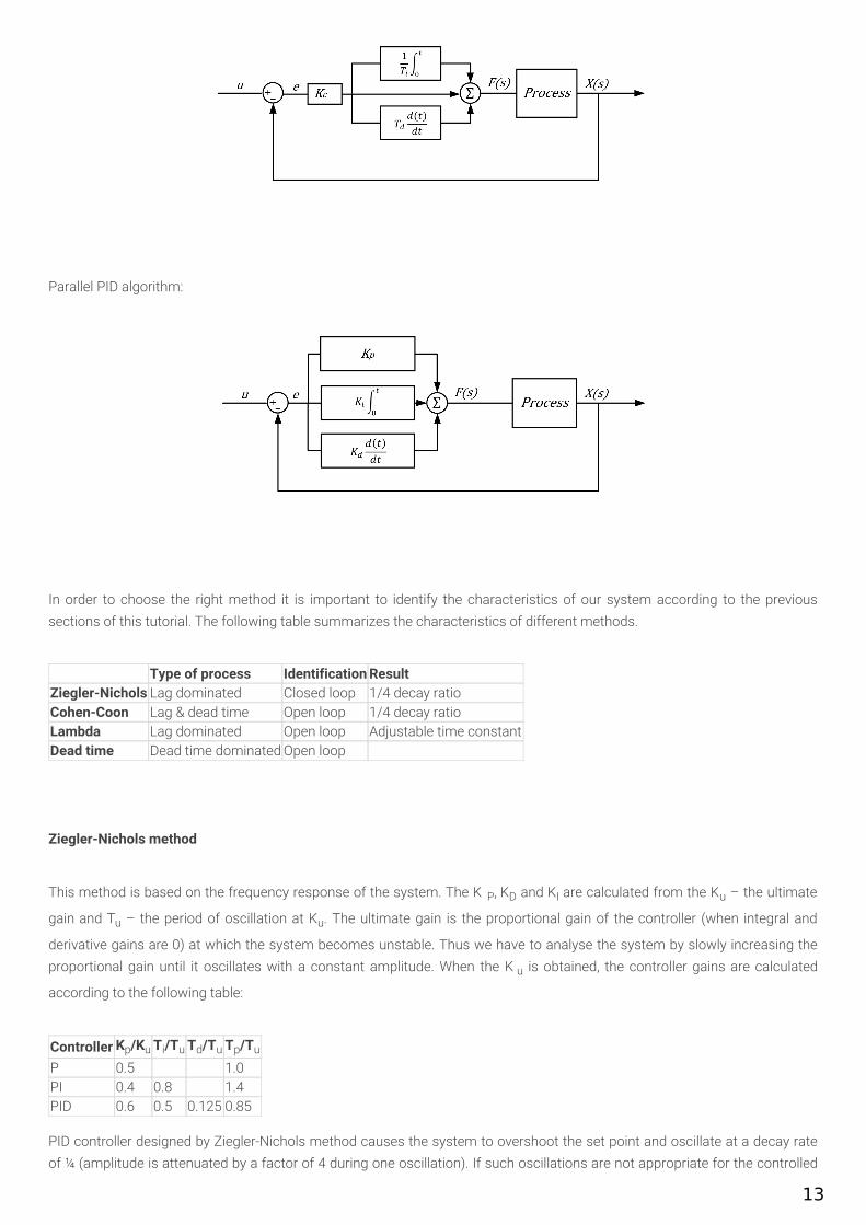
Parallel PID algorithm:

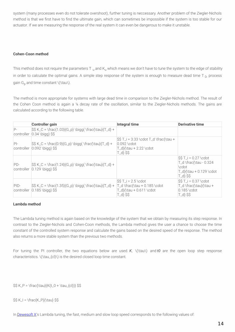
In order to choose the right method it is important to identify the characteristics of our system according to the previoussections of this tutorial. The following table summarizes the characteristics of different methods.

Type of process Identification ResultZiegler-Nichols Lag dominated Closed loop 1/4 decay ratioCohen-Coon Lag & dead time Open loop 1/4 decay ratioLambda Lag dominated Open loop Adjustable time constantDead time Dead time dominated Open loop

Ziegler-Nichols method

This method is based on the frequency response of the system. The K P, KD and KI are calculated from the Ku – the ultimate

gain and Tu – the period of oscillation at Ku. The ultimate gain is the proportional gain of the controller (when integral and

derivative gains are 0) at which the system becomes unstable. Thus we have to analyse the system by slowly increasing theproportional gain until it oscillates with a constant amplitude. When the K u is obtained, the controller gains are calculated

according to the following table:

Controller Kp/Ku Ti/Tu Td/Tu Tp/Tu

P 0.5 1.0PI 0.4 0.8 1.4PID 0.6 0.5 0.125 0.85

PID controller designed by Ziegler-Nichols method causes the system to overshoot the set point and oscillate at a decay rateof ¼ (amplitude is attenuated by a factor of 4 during one oscillation). If such oscillations are not appropriate for the controlled

13

system (many processes even do not tolerate overshoot), further tuning is neccessary. Another problem of the Ziegler-Nicholsmethod is that we rst have to nd the ultimate gain, which can sometimes be impossible if the system is too stable for ouractuator. If we are measuring the response of the real system it can even be dangerous to make it unstable.

Cohen-Coon method

This method does not require the parameters T u and Ku which means we don't have to tune the system to the edge of stability

in order to calculate the optimal gains. A simple step response of the system is enough to measure dead time T 0, process

gain Gp and time constant \(\tau\).

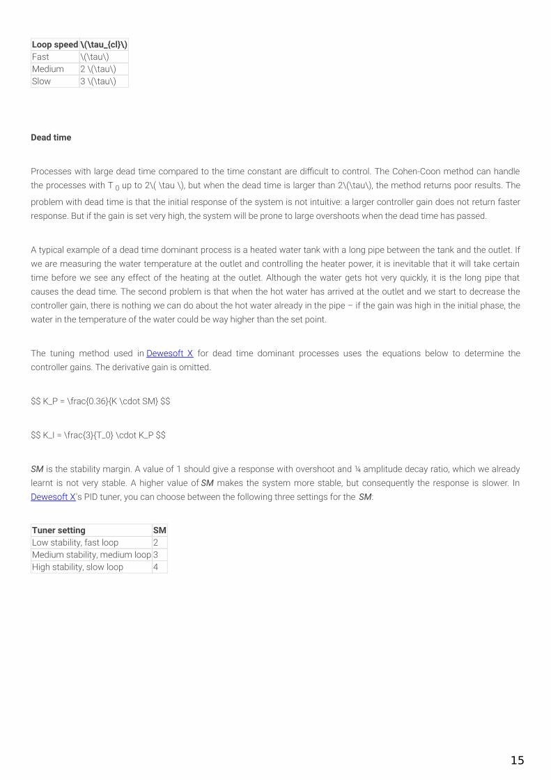
The method is more appropriate for systems with large dead time in comparison to the Ziegler-Nichols method. The result ofthe Cohen Coon method is again a ¼ decay rate of the oscillation, similar to the Ziegler-Nichols methods. The gains arecalculated according to the following table.

Controller gain Integral time Derivative timeP-controller

$$ K_C = \frac{1.03}{G_p} \bigg( \frac{\tau}{T_d} +0.34 \bigg) $$

PI-controller

$$ K_C = \frac{0.9}{G_p} \bigg( \frac{\tau}{T_d} +0.092 \bigg) $$

$$ T_i = 3.33 \cdot T_d \frac{\tau +0.092 \cdotT_d}{\tau + 2.22 \cdotT_d} $$

PD-controller

$$ K_C = \frac{1.24}{G_p} \bigg( \frac{\tau}{T_d} +0.129 \bigg) $$

$$ T_i = 0.27 \cdotT_d \frac{\tau - 0.324\cdotT_d}{\tau + 0.129 \cdotT_d} $$

PID-controller

$$ K_C = \frac{1.35}{G_p} \bigg( \frac{\tau}{T_d} +0.185 \bigg) $$

$$ T_i = 2.5 \cdotT_d \frac{\tau + 0.185 \cdotT_d}{\tau + 0.611 \cdotT_d} $$

$$ T_i = 0.37 \cdotT_d \frac{\tau}{\tau +0.185 \cdotT_d} $$

Lambda method

The Lambda tuning method is again based on the knowledge of the system that we obtain by measuring its step response. Incontrast to the Ziegler-Nichols and Cohen-Coon methods, the Lambda method gives the user a chance to choose the timeconstant of the controlled system response and calculate the gains based on the desired speed of the response. The methodalso returns a more stable system than the previous two methods.

For tuning the PI controller, the two equations below are used. K, \(\tau\) and t0 are the open loop step responsecharacteristics. \(\tau_{cl}\) is the desired closed loop time constant.

$$ K_P = \frac{\tau}{K(t_0 + \tau_{cl})} $$

$$ K_I = \frac{K_P}{\tau} $$

In Dewesoft X's Lambda tuning, the fast, medium and slow loop speed corresponds to the following values of:

14

Loop speed \(\tau_{cl}\)Fast \(\tau\)Medium 2 \(\tau\)Slow 3 \(\tau\)

Dead time

Processes with large dead time compared to the time constant are di cult to control. The Cohen-Coon method can handlethe processes with T 0 up to 2\( \tau \), but when the dead time is larger than 2\(\tau\), the method returns poor results. The

problem with dead time is that the initial response of the system is not intuitive: a larger controller gain does not return fasterresponse. But if the gain is set very high, the system will be prone to large overshoots when the dead time has passed.

A typical example of a dead time dominant process is a heated water tank with a long pipe between the tank and the outlet. Ifwe are measuring the water temperature at the outlet and controlling the heater power, it is inevitable that it will take certaintime before we see any effect of the heating at the outlet. Although the water gets hot very quickly, it is the long pipe thatcauses the dead time. The second problem is that when the hot water has arrived at the outlet and we start to decrease thecontroller gain, there is nothing we can do about the hot water already in the pipe – if the gain was high in the initial phase, thewater in the temperature of the water could be way higher than the set point.

The tuning method used in Dewesoft X for dead time dominant processes uses the equations below to determine thecontroller gains. The derivative gain is omitted.

$$ K_P = \frac{0.36}{K \cdot SM} $$

$$ K_I = \frac{3}{T_0} \cdot K_P $$

SM is the stability margin. A value of 1 should give a response with overshoot and ¼ amplitude decay ratio, which we alreadylearnt is not very stable. A higher value of SM makes the system more stable, but consequently the response is slower. InDewesoft X's PID tuner, you can choose between the following three settings for the SM:

Tuner setting SMLow stability, fast loop 2Medium stability, medium loop 3High stability, slow loop 4

15

Controlling the propeller rotational frequency in DewesoftXA two-blade propeller was mounted to a DC motor. The DC motor was driven by a PWM circuit, which was controlled by theanalog signal out of the analog out channel of the Dewesoft Sirius. Rotational encoder was connected to the back end of themotor shaft and used as a feedback sensor. The sensor was connected to the counter channel of the Dewesoft Sirius. Thefigure below schematically shows the setup.

The PWM generator we used is only capable of generating unipolar voltage, which means we cannot brake the propeller. It isnot ideal, but the propeller has a tendency to decrease its speed quite fast so it is not really problematic. Therefore when thecontrol voltage from the output channel is negative, the voltage at the motor is zero.

We want to control the rotational frequency by applying the right voltage to the motor. The rst step is to measure theresponse of the system to the step voltage input. We will be using the following variables in the process.

Variable Description Dewesoft channel nameProcess variable Rotational frequency of the propeller Propeller rotational frequency [RPM]Controller variable Voltage at the Analog Out channel Control AO voltage [-10 ... 10 V]Controller variable feedback Actual voltage at the Analog Out channel AO voltage feedback [-10 ... 10 V]

Note that we will be measuring the actual control voltage at the analog output connector. This is because there is a delaybetween the software command (Control AO voltage) and the actual output channel response due to the operating system –remember that Windows is not a real-time system. To minimize this delay, set the PID Loop Output Time to 0,01 s (10 ms) inthe PID Control Setup. The software will thus update the Controller variable at this rate. Typical delay of the operating systemwill be between 20 and 30 ms.

Note: in case you are controlling a very slow process like air temperature in a room, you could set the PID loop output time to alarger value to decrease the number of small valve actuations.

16

The first we can do is to model the system on paper. We want to find the voltage to rotational frequency transfer function forour system. The DC motor torque can be modeled by:

$$ T_P = \frac{k_T \cdot U}{R} - \frac{k_i \cdot \omega}{R} $$

kT(motor torque constant), ki (a product of kT and ke, the back-emf constant) and R (motor winding resistance) are motor

constants, but we are now interested in the variables that change with time (voltage U, rotational frequency ω, torque TP). We

will rewrite the motor torque equation with the constants merged:

$$ T_P = C_T \cdot U - C_i \cdot \omega $$

The torque from air drag that is opposing the motor torque can be modeled by:

$$ T_D = C_Q \cdot \omega^2 $$

CQ is a constant depending on propeller parameters like diameter, number of blades, lift and drag coefficient of the propeller

airfoil, twist etc. The equation of motion for the system can be written as follow:

$$ T_P - T_D = \dot{\omega} \cdot J_P $$

JP is the mass moment of inertia of the propeller, again a constant. Combining the equations we arrive at the following

expression:

$$ \dot{\omega} = \frac{1}{J_P} \bigg( C_T U - C_i \omega - C_Q \omega^2 \bigg)$$

The system is not linear since the aerodynamic drag is proportional to the square of the velocity. It is common practice inlinear control theory to linearize the equations about a certain steady state condition. Then the linearized equation is valid forsmall steps about this condition. The optimal gains then depend on the initial condition, but that can be solved with the socalled gain scheduling: a map of gains for many different conditions of operation. For example, the ight control algorithm ofthe F16 ghter aircraft uses gain scheduling to address hundreds of ight conditions with a linear controller. Dewesoft X PIDat the moment does not support gain scheduling directly, but one could try to implement it with the help of the sequencer forsome slow process control.

Coming back to our propeller model, if we linearize the system about the condition of ω = 0 and combine the constants intonew constants, we get:

$$ \dot{\omega} = K_U U - K_{\omega} \omega $$

This equation can be transformed to the frequency domain to arrive at the following transfer function:

$$ \frac{\omega(s)}{U(s)} = \frac{K_U}{s + K_{\omega}} $$

Click for full derivation

17

In order to linearize the equation of motion, we expand it into a Taylor series. We only consider the first two terms of theTaylor series:$$ f(\vec{x}) = f(\vec{x_0}) + f_{\vec{x1}}(\vec{x_0}) \cdot \Delta \vec{x} $$f represents the function we are linearizing (rotational acceleration). x is the vector of all variables in the function which inour case are ω and U. fx1x1 is the first derivative of the function with respect to the variables. The linearized function is

similar to the original function only for small perturbations of vector x about the linearization point x0 (hence Δ x). Thepoint about which we will linearize the function is U = 0, ω = 0. Taking the first derivative of f we get:$$ \dot{\omega}_{lin} = f(\vec{x_0}) + \frac{1}{J_P} C_T \cdot \Delta U - \frac{1}{J_P} \bigg (C_i + C_Q \omega \bigg)_0\Delta \omega $$f(x0x0) is zero at our linearization point. The value in brackets is a constant (the value of the derivative at the linearizationpoint) that we denote Kω. We also denote the product in front of U as a new constant KU. Keeping in mind that the

function represents our system for small perturbations of the variables, we can simplify:$$ \dot{\omega} = K_U \cdot U - K_{\omega} \cdot \omega $$From here we perform the Laplace transform:$$ \omega_{(s)} s = K_U U_{(s)} - K_{\omega} \omega_{(s)} $$Rearranging gives us the transfer function:$$ \frac{\omega_{(s)}}{U_{(s)}} = \frac{K_U}{s + K_{\omega}} $$

We immediately recognize the equation of a rst order system. The two constants depend on the motor windings andpropeller geometry, but we don't have to bother with that since the time constant and process gain of the system are easilyobtained by measuring the step response, which is our next step.

In the PID Control setup, we choose the Open Loop option to disable the feedback loop and the controller.

Our initial condition will be at the control voltage value of 1 V when the propeller rotates at about 670 RPM. This is due to thefact that the encoder we are using is not very accurate at low RPM (it has a resolution of 1024 points per rotation). We willintroduce a 1.5 V step in control voltage (from 1 V to 2.5 V) and measure the open loop response.

The result is a typical rst order system response. As seen on the gure above the time constant of the system is about 415ms. The rst cursor is placed at the step of the controller output voltage (purple line). The second cursor is placed at the pointwhere the frequency reaches 63% of the nal value. Dewesoft X displays the time between the cursors at the bottom rightcorner of the screen.

The dead time of this process is very low, about 0.6 ms, which can also be measured from the step response. Such a low deadtime is negligible for our purpose so we will assume the process has zero dead time. We will arti cially introduce longer dead

18

time later in this tutorial to see its effect on the system.

From this knowledge of the system we select the Ziegler-Nichols and Lambda method for the tuning of the controller. TheCohen Coon method is appropriate for the systems with larger time constant while the Dead Time method is appropriate forthe systems with large dead time – both of which is not true for our system.

19

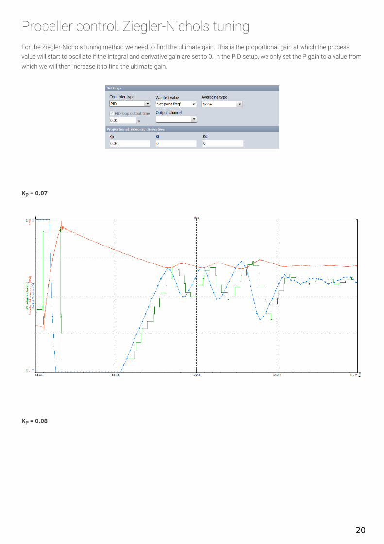
Propeller control: Ziegler-Nichols tuningFor the Ziegler-Nichols tuning method we need to find the ultimate gain. This is the proportional gain at which the processvalue will start to oscillate if the integral and derivative gain are set to 0. In the PID setup, we only set the P gain to a value fromwhich we will then increase it to find the ultimate gain.

KP = 0.07

KP = 0.08

20

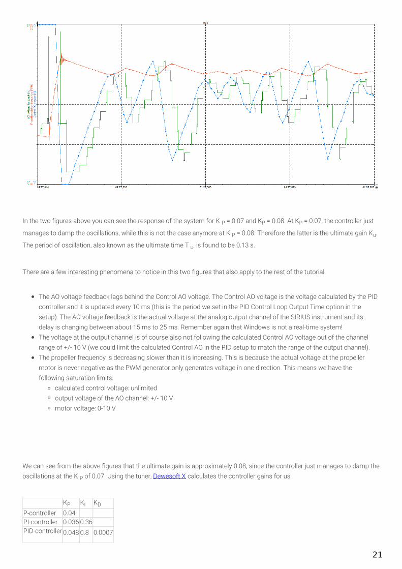
In the two figures above you can see the response of the system for K P = 0.07 and KP = 0.08. At KP = 0.07, the controller just

manages to damp the oscillations, while this is not the case anymore at K P = 0.08. Therefore the latter is the ultimate gain Ku.

The period of oscillation, also known as the ultimate time T u, is found to be 0.13 s.

There are a few interesting phenomena to notice in this two figures that also apply to the rest of the tutorial.

The AO voltage feedback lags behind the Control AO voltage. The Control AO voltage is the voltage calculated by the PIDcontroller and it is updated every 10 ms (this is the period we set in the PID Control Loop Output Time option in thesetup). The AO voltage feedback is the actual voltage at the analog output channel of the SIRIUS instrument and itsdelay is changing between about 15 ms to 25 ms. Remember again that Windows is not a real-time system!The voltage at the output channel is of course also not following the calculated Control AO voltage out of the channelrange of +/- 10 V (we could limit the calculated Control AO in the PID setup to match the range of the output channel).The propeller frequency is decreasing slower than it is increasing. This is because the actual voltage at the propellermotor is never negative as the PWM generator only generates voltage in one direction. This means we have thefollowing saturation limits:

calculated control voltage: unlimitedoutput voltage of the AO channel: +/- 10 Vmotor voltage: 0-10 V

We can see from the above gures that the ultimate gain is approximately 0.08, since the controller just manages to damp theoscillations at the K P of 0.07. Using the tuner, Dewesoft X calculates the controller gains for us:

KP KI KD

P-controller 0.04PI-controller 0.036 0.36PID-controller 0.048 0.8 0.0007

21

The system responses of all controllers are pictured below:

P-controller

PI-controller

PID-controller

22

Before discussing the results we will first tune the controller with the Lambda method.

23

Propeller control: Lambda tuningTo use the Lambda tuning method we need to further analyse the step response of the system to calculate the process gainfrom the values of dCO and dPV. Note from the step response plot that the figures are:

dCO = 1.5 VdPV = 640 RPM

We already calculated the time constant (0.415 s) and dead time (0 s). With this data, the Lambda tuner in Dewesoft Xcalculates the following gains for the PI controller:

P-gain I-gain Option0.0022 0.0052 Fast0.0007 0.017 Slow

The response of the system for both options is plotted in the next two figures.

Fast

Slow

24

Note that the time scale on the plots is different than on the Ziegler-Nichols response plots because the Lambda response ismuch slower. The results are discussed in the following section.

25

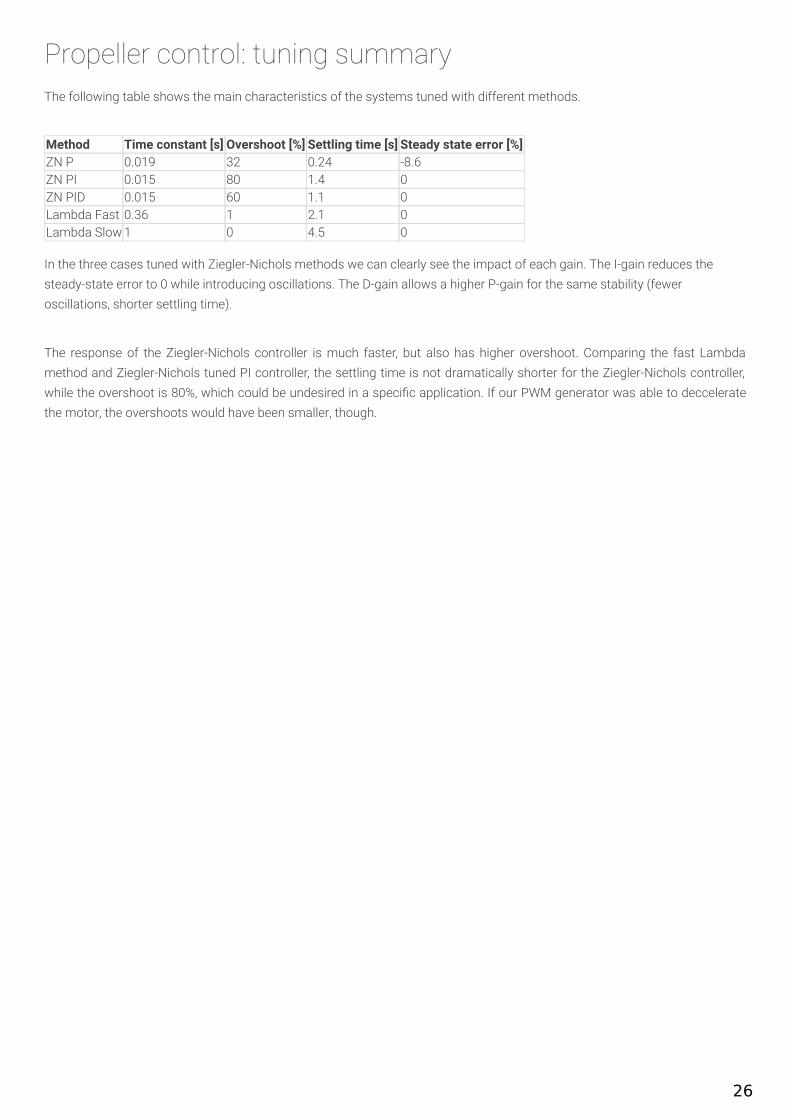
Propeller control: tuning summaryThe following table shows the main characteristics of the systems tuned with different methods.

Method Time constant [s] Overshoot [%] Settling time [s] Steady state error [%]ZN P 0.019 32 0.24 -8.6ZN PI 0.015 80 1.4 0ZN PID 0.015 60 1.1 0Lambda Fast 0.36 1 2.1 0Lambda Slow 1 0 4.5 0

In the three cases tuned with Ziegler-Nichols methods we can clearly see the impact of each gain. The I-gain reduces thesteady-state error to 0 while introducing oscillations. The D-gain allows a higher P-gain for the same stability (feweroscillations, shorter settling time).

The response of the Ziegler-Nichols controller is much faster, but also has higher overshoot. Comparing the fast Lambdamethod and Ziegler-Nichols tuned PI controller, the settling time is not dramatically shorter for the Ziegler-Nichols controller,while the overshoot is 80%, which could be undesired in a speci c application. If our PWM generator was able to decceleratethe motor, the overshoots would have been smaller, though.

26

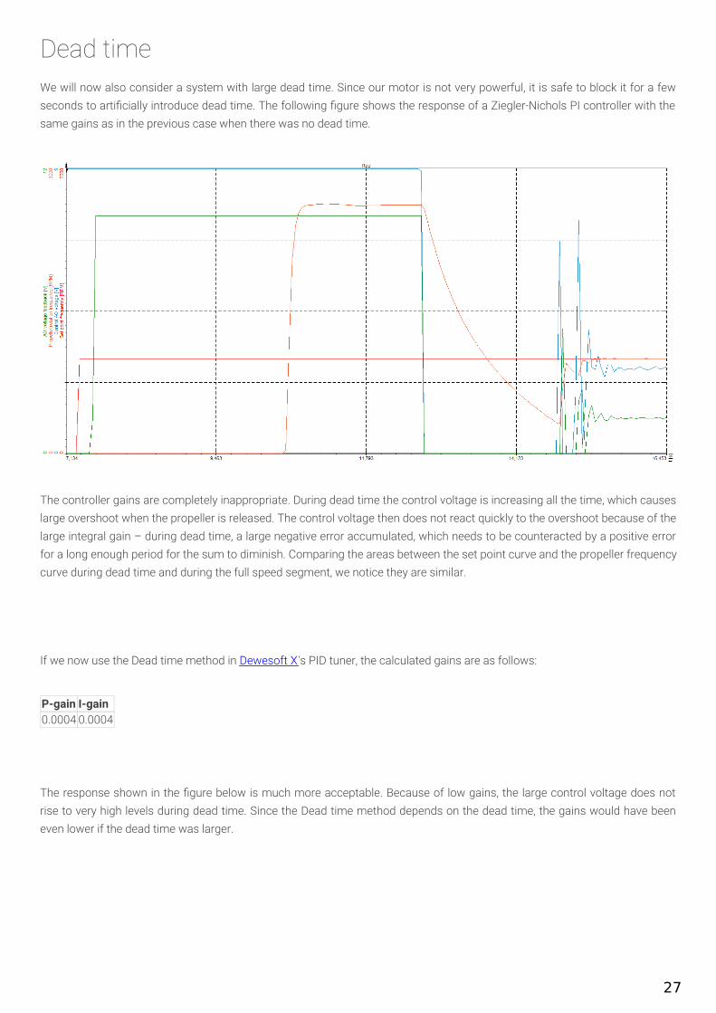
Dead timeWe will now also consider a system with large dead time. Since our motor is not very powerful, it is safe to block it for a fewseconds to arti cially introduce dead time. The following gure shows the response of a Ziegler-Nichols PI controller with thesame gains as in the previous case when there was no dead time.

The controller gains are completely inappropriate. During dead time the control voltage is increasing all the time, which causeslarge overshoot when the propeller is released. The control voltage then does not react quickly to the overshoot because of thelarge integral gain – during dead time, a large negative error accumulated, which needs to be counteracted by a positive errorfor a long enough period for the sum to diminish. Comparing the areas between the set point curve and the propeller frequencycurve during dead time and during the full speed segment, we notice they are similar.

If we now use the Dead time method in Dewesoft X's PID tuner, the calculated gains are as follows:

P-gain I-gain0.0004 0.0004

The response shown in the gure below is much more acceptable. Because of low gains, the large control voltage does notrise to very high levels during dead time. Since the Dead time method depends on the dead time, the gains would have beeneven lower if the dead time was larger.

27

28

Integrator windupThere is another way to conquer large dead time. In the PID setup we can choose the PI (anti-windup) controller type. This willprevent the accumulation of the integration error when the actuator is in saturation, which happens during dead time. If thistype of controller is chosen, the Ziegler-Nichols method provides very good response also in case of a large dead time ( gurebelow). Note that the control voltage stops increasing when the controller notices that there is no response of the processvariable (propeller frequency).

We have to set the windup limits of the output channel in the setup for the anti-windup to function properly. A practical valuewould be just below the actuator saturation level.

29