Volume 35 (2), pp. 161–186

http://orion.journals.ac.za

ORiONISSN 0259–191X (print)ISSN 2224–0004 (online)

c©2019

Picking location metrics for order batching on aunidirectional cyclical picking line

FM Hofmann∗ SE Visagie†

Received: 18 March 2019; Revised: 5 July 2019; Accepted: 25 July 2019

Abstract

In this paper order batching is extended to a picking system with the layout of aunidirectional cyclical picking line. The objective is to minimise the walking distanceof pickers in the picking line. The setup of the picking system under consideration isrelated to unidirectional carousel systems. Three order-to-route closeness metrics areintroduced to approximate walking distance, since the orders will be batched beforethe pickers are routed. All metrics are based on the picking location describing when apicker has to stop at a location to collect the items for an order. These metrics comprisea number of stops, a number of non-identical stops and a stops ratio measurement.Besides exact solution approaches, four greedy heuristics as well as six metaheuristicsare applied to combine similar orders in batches. All metrics are tested using real lifedata of 50 sample picking lines in a distribution centre of a prominent South Africanretailer. The capacity of the picking device is restricted, thus the maximum batchsize of two orders per batch is allowed. The best combination of metric and solutionapproach is identified. A regression analysis supports the idea that the introducedmetrics can be used to approximate walking distance. The combination of stops ratiometric and the greedy random heuristic generate the best results in terms of minimumnumber of total cycles traversed as well as computational time to find the solution.

Key words: Order batching, picking location metrics, unidirectional cyclical picking line, carousel

1 Introduction

The need for greater product variety and shorter response times emphasises a companies’ability to establish efficient logistical operations. This efficiency is, amongst others, de-termined by the operation of its warehouses or distribution centres (DC) that define the

∗Department of Logistics, Stellenbosch University, South Africa, email: 20304269@sun.ac.za†Corresponding author: (Fellow of the Operations Research Society of South Africa) Depart-

ment of Logistics, Stellenbosch University, South Africa, email: svisagie@sun.ac.za

http://dx.doi.org/10.5784/35-2-646

161

162 FM Hofmann & SE Visagie

nodes in the distribution network [48]. In a supply chain connecting production plantswith end customers warehousing cannot be eliminated. The role of warehouse operationsis constantly changing and thus has to remain flexible. A DC focuses on the consolida-tion and accumulation of numerous products from various suppliers to many customers.Products from different suppliers arrive in bulk at the DC. The stock is then turned intocustomer or store orders for delivery to the DC’s customers [18].

Van den Berg & Zijm [54] subdivide DC activities into four categories namely receiving,storage, order picking and shipping. From the total logistics cost of a company, approx-imately 25% can be attributed to the cost of operating a warehouse [23]. Therein, thebasic service of a DC is order picking that makes up for 50% to 65% of the operationalcost accounting for labour, capital and supporting activities [54]. De Koster et al. [12]define the process of order picking as retrieving products from storage or buffer areas andturning them into specific orders in response to a customer request. The design of theorder picking system is crucial to its performance. The number of orders together withthe items per order that are picked in a day, the average size of an order and the layoutof the storage racks are key parameters to set up an efficient order picking system [10].

The order picking system of a prominent South African retailer (referred to as the Retailer)with around 2 000 outlets or stores is considered here. A set of non-uniform orders is theresult of a large number of stores with different sizes and various customer profiles thatneeds to be handled by the DC on a daily basis. A key characteristic of the Retailer’soperations is the central planning of the inventory kept at a store level. Instead of stockrequested by store managers, planners at a central planning department assign stock thatis available at the DC to stores. Thereby, the central planning department allocates stockkeeping units (SKUs) to stores. Planners in the central planning department decide on thenumber of SKUs destined for each store after the arrival of the SKUs at the DC. Plannersissue instructions to the DC about the SKUs and the stores where they should go. TheDC then selects a subset of SKUs to be picked in a single picking wave to satisfy all storerequirements for that set of SKUs. In this study, the term order will thus refer to the setof store requirements for a single store for all SKUs selected to be processed in a wave. Awave is processed on a picking line in the DC. A single SKU is assigned to a single locationon a specific picking line for each wave. The activities of populating the line with SKUs,the actual picking process and removing excess stock from the line comprise a pickingwave [36].

Locations

Locations

Conveyor Belt

m21

m i

Figure 1: A schematic representation of a picking line with m locations.

Picking location metrics for order batching 163

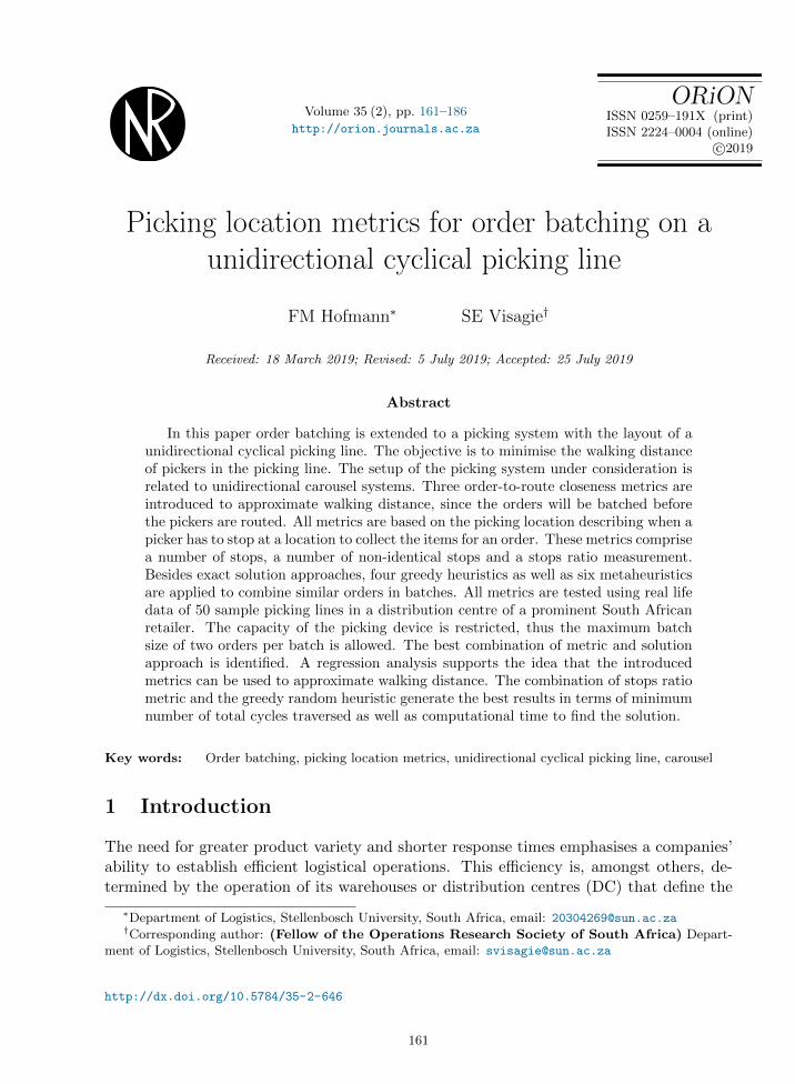
A schematic representation of a picking line with m locations is depicted in Figure 1. Atthe Retailer’s DC a picking line consists of 56 locations with a conveyor belt placed inthe middle that has two access gates. From the storage area, a single SKU is assigned toa single location on the picking line. The number of items of each SKU to be picked forall stores are known prior to the start of a picking wave. Each location has the storagecapacity of five pallets of an identical SKU. Additional stock is kept on the floor spacebetween different picking lines for easy refill avoiding stock-outs. Therefore, stock doesnot have to be replenished from storage racks during a picking wave. Pickers move aroundthe conveyor belt in a clockwise direction picking all orders. A voice recognition system(VRS) guides the pickers through the picking process by sending a picker to the closestrequired SKU. Therefore, the underlying picking strategy can be summarised as pick theclosest SKU in a clockwise direction. The picking system is categorised as a picker-to-partssystem. Before the picking of an order is started, an empty carton is placed on the trolleyand registered through a barcode with the VRS. After picking, full cartons and finishedorders are placed on the conveyor belt for further processing in the dispatch area of theDC [34, 35].

The setup of the picking system at the DC shows many similarities to unidirectionalcarousel systems, if the SKUs are viewed as moving relative to a static picker. A carousel isan automated warehouse system that can be used for picking small and medium products.It is designed as a rotatable circuit of shelving holding multiple SKUs. A picker, whoremains at a fixed location during the picking process, operates the system. In literaturethis picking system is referred to as a parts-to-picker system, since the storage locationtravels to the picker instead of the picker travelling to the storage location. A bidirectionalcarousel can rotate in both directions to bring the required SKU in front of the picker,whereas a unidirectional carousel can only move in one direction [3]. The cyclical setupof the picking line and the assumptions that one picker processes one order as well as theautomation of pick sequencing by the VRS resembles a unidirectional carousel. However,the presence of wave picking is the main difference in the Retailer’s system to the carouselsystems studied in literature. Not all SKUs may be picked and new orders may be added tothe set during the picking operation in typical carousel systems. Therefore, optimisationapproaches make use of expected SKU mixes in orders that are derived from historicaldata [33]. The deterministic nature of the orders (because all orders are known and fixedwhen a wave of picking starts) is unique to the Retailer’s picking system in operationsresearch literature [36].

Planning for order picking includes the order batching problem. Orders that are requestedare subsequently released for fulfilment. This set of orders needs to be picked and accumu-lated for packing and shipping in a picking wave [22]. The combination of customer ordersinto picking orders describes the process of order batching [24]. According to Wascher[55] order batching answers the question of how customer orders should be grouped intopicking orders to minimise the total length of all picking tours necessary to collect all itemswhile no customer order is split, given a set of customer orders consisting of a number ofitems, an assignment of items to storage locations in the order picking system of a ware-house and the capacity of a picking device. Tours that efficiently shorten the picking timecan be generated, since several orders are picked simultaneously leading to a reduction inlabour cost [11].

164 FM Hofmann & SE Visagie

While there has been intensive research on the order batching problem in single-blockwarehouses with parallel aisles, according to Nicolas et al. [42] little research has beenpublished on carousel systems. The literature on carousels can be categorised into eitherdetermining the pick sequence on a carousel or finding the best storage location for aproduct in a carousel. No study on order batching applied to a manual unidirectionalcarousel systems as implemented by the Retailer could be found in literature.

This study aims at answering the question if the order batching problem (OBP) can beapplied to the specific layout of a unidirectional cyclical picking line. The orders will bebatched before the pickers are routed. However, walking distance can not be determineda priori and thus a realistic approximation for distance has to be provided. Differentlocation-based metrics are thus developed to estimate walking distance, since calculatingwalking distance is too time consuming. Different algorithms that correlate with thesemetrics to solve the order batching problem are tested. A suggested combination of metricand algorithm to minimise the total distance travelled by a picker to collect all ordersduring a picking wave concludes the study.

A brief overview on the literature of order-batching in single-block and automated storageand retrieval warehouse setups is given in Section 2. The model will be described inSection 3 including assumptions, measurements and an integer programming formulationof the problem. The location-based order-to-route closeness metrics will be proposed inSection 4. In Section 5 different heuristic approaches comprised of greedy heuristics andmetaheuristics are introduced to solve the OBP in reasonable time. A case study withreal life data from the Retailer is used to test the performance of the combinations ofmetrics and algorithms in Section 6. In Section 7 a summary as well as an outlook onfuture research opportunities is provided.

2 Literature review

The formulation of the standard order batching problem (OBP) was introduced and provedto be NP-hard in the strong sense by Gademann & Velde [19] for a single-block warehousewith parallel aisles. However, if no batch contains more than two orders the problem canbe solved in polynomial time. The branch-and-prize algorithm developed by Gademann& Velde [19] solved test instances of up to 32 orders to optimality. Additionally, Henn &Wascher [25] solved instances of up to 40 orders. Nevertheless, their solution approachrequired a time-consuming preprocessing of all feasible batches. Furthermore, Muter &Oncan [41] solved instances of up to 100 orders with their specially tailored column-generation based algorithm. In practice the number of customer orders is likely to exceedthese test instances, but the exact algorithms proposed so far are not able to consistentlysolve larger instances. Nicolas et al. [42] introduced the OBP to a vertical carousel systemthat is closely related to the layout of the unidirectional cyclical picking line. The OBPis formulated as a mixed integer linear program (MILP). Nevertheless, the MILP has tobe stopped after 30 minutes due to time constraints for test instances over 50 orders. Inthe Retailer’s DC a picking line can service up to 1 500 orders. Larger problem instancesmust be solved using heuristics. Therefore, construction heuristics like seed algorithmsand saving algorithms have been introduced to solve the OBP.

Picking location metrics for order batching 165

A straight-forward heuristic is the first-come-first-served method that groups together thefirst entries of the list of orders as close as possible to the predetermined maximum batchsize. Then the next orders are grouped using a similar logic until all orders form part ofa batch [20].

Seed algorithms start by initiating batches, then allocating orders to batches and terminatethrough a stopping rule when a batch has been completed. The objective is to minimisethe total travel distance for collecting all orders. De Koster et al. [11] evaluated seedalgorithms in a parallel aisle warehouse proposing the seed selection rules of the fartheststorage location. Ho & Tseng [27] investigated several location- and aisles-based seedalgorithms in the standard OBP environment of a single-block parallel aisle warehouse.Ho et al. [26] extended this study with further distance- and area-based selection rules inthis environment. In their comparative study Pan & Liu [45] evaluated four initial seedselection and four order addition rules investigating the OBP in an automated storage andretrieval system that consists of a single storage rack with equally sized storage locationsserviced by a single storage and retrieval machine.

Saving algorithms in the OBP are based on the Clarke and Wright-algorithm (CW) [9] andthus the time saving that can be obtained by comparing the collection of orders in one routeto individual picking [11]. The minimum additional aisles heuristic proposed by Rosenwein[47] starts with calculating a score for each pair of orders in terms of additional aisles topick from in the cases that orders are picked simultaneously or separately. Therefore,their algorithm is capable of generating fewer but shorter picking tours when comparedto Gibson & Sharp [20]. The first OBP version of the algorithm (CW i) described byDe Koster et al. [11] computes savings for each combination of orders. Each time a newcombination of orders to batches has been determined the savings are recalculated in thesecond version of the algorithm (CW ii). Bozer & Kile [6] improved this version of thealgorithm by introducing a normalised time saving value for each pair of orders. Eachtime an order has been assigned the initial savings matrix is modified resulting in a thirdversion (CW iii) proposed by De Koster et al. [11]. Additionally, Elsayed & Unal [17]proposed a small and large algorithm. Therefore, orders are either classified as small orlarge according to a predefined value before they are assigned to batches. In general seedalgorithms are more central processing unit (CPU) time saving than saving algorithms.The order-to-route closeness metric is central to all types of heuristics [22].

Metaheuristics are designed to solve a wide range of hard optimisation problems and canthus also be applied to the OBP. An iterated local search that explores a neighbourhoodto identify a new solution with a smaller objective function value was applied to the OBPby Henn et al. [23]. Albareda-Sambola et al. [2] defined three neighbourhoods to introducethe OBP to a variable neighbourhood search. A tabu search that simulates the humanmemory processes including a tabu list was applied to the OBP by Henn & Wascher[25]. Matusiak et al. [38] introduced a simulated annealing approach that simulates thecooling process of metal to the OBP. Moreover, Oncan [43] introduced a combination ofan iterated local search with a tabu threshold to the OBP. A hybrid of a large adaptiveneighbourhood search and a tabu search was developed by Zulj et al. [56] based on thefindings of Henn & Wascher [25] and Oncan [43].

166 FM Hofmann & SE Visagie

3 Model formulation

The problem environment of this study is a DC of the Retailer. The DC is made up ofseveral unidirectional cyclical picking lines functioning in parallel. Thus one such pickingline will be in the centre of attention. This layout differs significantly from the parallel-aisle or the single-aisle automated storage and retrieval warehouses that are frequentlystudied in academic literature.

The following assumptions are made while modelling the Retailer’s order picking system.

1. The orders that need to be picked during a wave as well as the SKUs and theirlocation in the picking line will be fixed a priori.

2. For movability the picking devices are small. However, SKUs are generally bulky.Therefore, the capacity of the picking devices is currently restricted to accommodatetwo orders at a time restricting the batch size to two.

3. A picker must complete the entire order before starting the next, packing stockdirectly onto the trolley. When an order is completed or the carton is full, it isplaced on the conveyor belt for further processing.

4. It is assumed that a picker walks at a constant speed and that the time taken topick and pack a SKU or switch between orders is constant.

3.1 Measurements

The cycles traversed measurement, that was introduced by Matthews & Visagie [36],counts the number of cycles that have to be traversed to pick all items requested duringa picking wave as a measure of distance travelled to pick all orders. This measurementcounts the total number of cycles required to pick and link all orders.

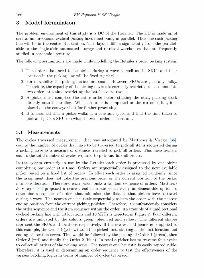
In the system currently in use by the Retailer each order is processed by one pickercompleting one order at a time. Orders are sequentially assigned to the next availablepicker based on a fixed list of orders. In effect each order is assigned randomly, sincethe assignment does not take the previous order or the current position of the pickerinto consideration. Therefore, each picker picks a random sequence of orders. Matthews& Visagie [36] proposed a nearest end heuristic as an easily implementable option todetermine a sequence of orders that minimises the distance that pickers have to travelduring a wave. The nearest end heuristic sequentially selects the order with the nearestending position from the current picking position. Therefore, it simultaneously considersthe order sequence and the item sequence within the order. An example of a unidirectionalcyclical picking line with 10 locations and 10 SKUs is depicted in Figure 2. Four differentorders are indicated by the colours green, blue, red and yellow. The different shapesrepresent the SKUs and locations respectively. If the nearest end heuristic is applied tothis example, the Order 4 (yellow) would be picked first, starting at the first location andending at location seven. This would be followed by the picking of Order 1 (green), thenOrder 3 (red) and finally the Order 2 (blue). In total a picker has to traverse four cyclesto collect all orders of the picking wave. The nearest end heuristic is easily reproducible.Therefore, it is used in determining an order sequence to test the effectiveness of thevarious batching logics in terms of number of cycles traversed.

Picking location metrics for order batching 167

Figure 2: Schemantic representation of a picking line with 10 SKUs and 10 locations.

This study focuses on location-based order-to-route-closeness metrics. Each picking loca-tion defines where a picker has to stop at a location to pick items for an order. Differentpicking location or so-called stop metrics will be developed to identify compatible ordersin terms of number of stops in common. The assumption is that a good overlap in stopsmay lead to a reduction in total walking distance.

3.2 Exact formulation

Minimising the completion time is equivalent to minimising the travel distance to collectall orders in a picking wave. Therefore, the objective is to minimise the incompatibilityin terms of distance between orders that are described by a picking location metric toobtain the smallest number of cycles that have to be traversed. Orders must be combinedin batches of size two. This can be formulated as an integer programming model. Let

n be the number of orders,cij be the cost in terms of incompatible stops to batch order i and order j,

and define the set of variables as

xij =

{1, if order i and order j are in the same batch,

0, otherwise.

The objective is to

minimisen∑i=1

n∑j=i+1

cij xij (1)

168 FM Hofmann & SE Visagie

subject to

i−1∑k=1

xki +

n∑j=i+1

xij = 1 i = 1, . . . , n (2)

xij ∈ {0, 1}

{i = 1, . . . , n

j = i+ 1, . . . , n.(3)

The incompatibility between orders in terms of stops expressed by a picking location metricis minimised by objective function (1). The set of triangular inequality constraints (2) andthe binary condition (3) assign each order to only one other order in the case of a symmetriccost matrix.

The problem formulated in (1) – (3) is in essence an assignment problem. Another optionto solve the assignment problem is the quick match algorithm that was introduced by Orlin& Lee [44]. It is based on the successive shortest path algorithm and combines a forwardDijkstra with a reverse Dijkstra algorithm. Moreover, heuristics are included to speed upits performance. Therefore, this algorithm will also be included for testing purposes.

4 Picking location metrics

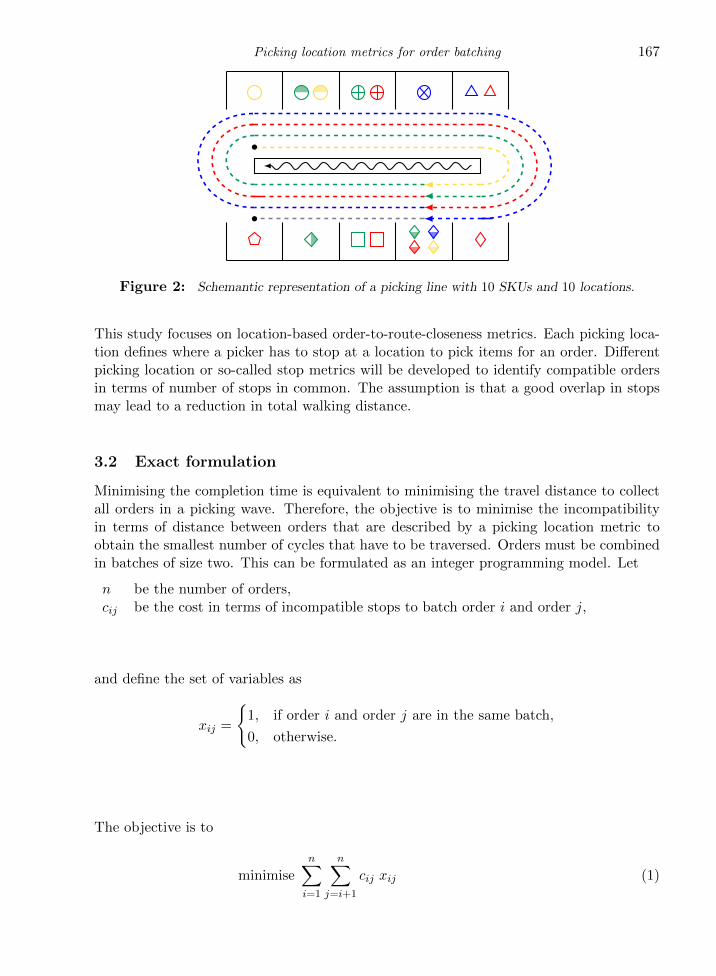
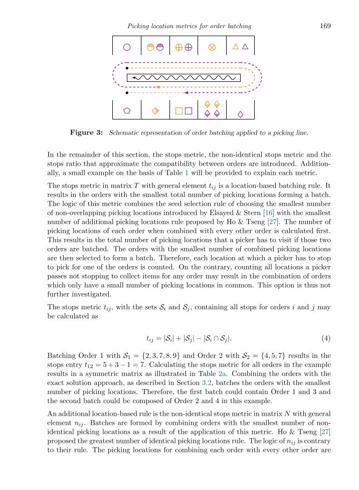
The simplest way of introducing order batching to a unidirectional cyclical picking linewould be to implement a first-in-first-out (FIFO) approach. According to the FIFO rulethe first entries of a list of orders are grouped together until the predetermined maximumbatch size is reached [20]. FIFO is often used in literature as a benchmark to comparedifferent batching methods. It will also be used here to compare the metrics that measurethe incompatibility of orders in terms of stops. An example of the picking locations of fourorders is illustrated in Table 1. Employing the nearest end heuristic as a routing strategy(Section 3.1), a picker has to traverse four cycles to collect all four orders. If FIFO isapplied as the random batching strategy and a batch is only allowed to contain two ordersas illustrated in Figure 3, then the first two orders would form batch one (in orange) andbatch two would be composed of Order 3 and Order 4 (in purple). The circles representthe movement of a picker showing that only two cycles have to be traversed. The numberof circles traversed will indicate the walking distance to compare different metrics.

Picking line location example

Locations: 1 2 3 4 5 6 7 8 9 10

Order 1Order 2Order 3Order 4

Table 1: The picking locations of the four orders.

Picking location metrics for order batching 169

Figure 3: Schematic representation of order batching applied to a picking line.

In the remainder of this section, the stops metric, the non-identical stops metric and thestops ratio that approximate the compatibility between orders are introduced. Addition-ally, a small example on the basis of Table 1 will be provided to explain each metric.

The stops metric in matrix T with general element tij is a location-based batching rule. Itresults in the orders with the smallest total number of picking locations forming a batch.The logic of this metric combines the seed selection rule of choosing the smallest numberof non-overlapping picking locations introduced by Elsayed & Stern [16] with the smallestnumber of additional picking locations rule proposed by Ho & Tseng [27]. The number ofpicking locations of each order when combined with every other order is calculated first.This results in the total number of picking locations that a picker has to visit if those twoorders are batched. The orders with the smallest number of combined picking locationsare then selected to form a batch. Therefore, each location at which a picker has to stopto pick for one of the orders is counted. On the contrary, counting all locations a pickerpasses not stopping to collect items for any order may result in the combination of orderswhich only have a small number of picking locations in common. This option is thus notfurther investigated.

The stops metric tij , with the sets Si and Sj , containing all stops for orders i and j maybe calculated as

tij = |Si|+ |Sj | − |Si ∩ Sj |. (4)

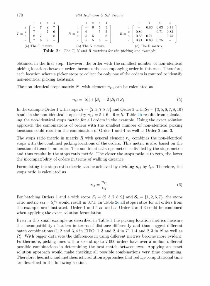
Batching Order 1 with S1 = {2, 3, 7, 8, 9} and Order 2 with S2 = {4, 5, 7} results in thestops entry t12 = 5 + 3− 1 = 7. Calculating the stops metric for all orders in the exampleresults in a symmetric matrix as illustrated in Table 2a. Combining the orders with theexact solution approach, as described in Section 3.2, batches the orders with the smallestnumber of picking locations. Therefore, the first batch could contain Order 1 and 3 andthe second batch could be composed of Order 2 and 4 in this example.

An additional location-based rule is the non-identical stops metric in matrixN with generalelement nij . Batches are formed by combining orders with the smallest number of non-identical picking locations as a result of the application of this metric. Ho & Tseng [27]proposed the greatest number of identical picking locations rule. The logic of nij is contraryto their rule. The picking locations for combining each order with every other order are

170 FM Hofmann & SE Visagie

T =

1 2 3 4

1 − 7 8 72 7 − 7 63 8 7 − 84 7 6 8 −

(a) The T matrix.

N =

1 2 3 4

1 − 6 5 52 6 − 5 53 5 5 − 64 5 5 6 −

(b) The N matrix.

R =

1 2 3 4

1 − 0.86 0.63 0.712 0.86 − 0.71 0.833 0.63 0.71 − 0.754 0.71 0.83 0.75 −

(c) The R matrix.

Table 2: The T, N and R matrices for the picking line example.

obtained in the first step. However, the order with the smallest number of non-identicalpicking locations between orders becomes the accompanying order in this case. Therefore,each location where a picker stops to collect for only one of the orders is counted to identifynon-identical picking locations.

The non-identical stops matrix N , with element nij , can be calculated as

nij = |Si|+ |Sj | − 2 |Si ∩ Sj |. (5)

In the example Order 1 with stops S1 = {2, 3, 7, 8, 9} and Order 3 with S3 = {3, 5, 6, 7, 8, 10}result in the non-identical stops entry n13 = 5 + 6− 6 = 5. Table 2b results from calculat-ing the non-identical stops metric for all orders in the example. Using the exact solutionapproach the combinations of orders with the smallest number of non-identical pickinglocations could result in the combination of Order 1 and 4 as well as Order 2 and 3.

The stops ratio metric in matrix R with general element rij combines the non-identicalstops with the combined picking locations of the orders. This metric is also based on thelocation of items in an order. The non-identical stops metric is divided by the stops metricand thus results in the stops ratio metric. The closer the stops ratio is to zero, the lowerthe incompatibility of orders in terms of walking distance.

Formulating the stops ratio metric can be achieved by dividing nij by tij . Therefore, thestops ratio is calculated as

rij =nijtij. (6)

For batching Orders 1 and 4 with stops S1 = {2, 3, 7, 8, 9} and S4 = {1, 2, 6, 7}, the stopsratio metric r14 = 5/7 would result in 0.71. In Table 2c all stops ratios for all orders fromthe example are illustrated. Order 1 and 4 as well as Order 2 and 3 could be combinedwhen applying the exact solution formulation.

Even in this small example as described in Table 1 the picking location metrics measurethe incompatibility of orders in terms of distance differently and thus suggest differentbatch combinations (1, 2 and 3, 4 in FIFO, 1, 3 and 2, 4 in T , 1, 4 and 2, 3 in N as well asR). With bigger data sets the differences in using different metrics become more evident.Furthermore, picking lines with a size of up to 2 000 orders have over a million differentpossible combinations in determining the best match between two. Applying an exactsolution approach would make checking all possible combinations very time consuming.Therefore, heuristic and metaheuristic solution approaches that reduce computational timeare described in the following section.

Picking location metrics for order batching 171

5 Heuristic solution approaches

After the orders have been measured using one of the proposed picking location metrics,different algorithms to combine the orders in batches of size two for a unidirectional cyclicalpicking line in the Retailer’s DC are described in this section. Four greedy heuristics aswell as six metaheuristics are introduced.

5.1 Greedy heuristics

The four different variations of greedy heuristics include a greedy top-down, a greedybottom-up, a greedy random and a greedy smallest entry approach. All four variationssearch through the symmetric matrices generated by applying the stop metrics for mini-mum entries.

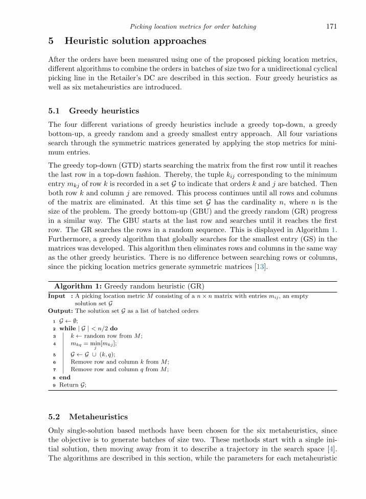
The greedy top-down (GTD) starts searching the matrix from the first row until it reachesthe last row in a top-down fashion. Thereby, the tuple kij corresponding to the minimumentry mkj of row k is recorded in a set G to indicate that orders k and j are batched. Thenboth row k and column j are removed. This process continues until all rows and columnsof the matrix are eliminated. At this time set G has the cardinality n, where n is thesize of the problem. The greedy bottom-up (GBU) and the greedy random (GR) progressin a similar way. The GBU starts at the last row and searches until it reaches the firstrow. The GR searches the rows in a random sequence. This is displayed in Algorithm 1.Furthermore, a greedy algorithm that globally searches for the smallest entry (GS) in thematrices was developed. This algorithm then eliminates rows and columns in the same wayas the other greedy heuristics. There is no difference between searching rows or columns,since the picking location metrics generate symmetric matrices [13].

Algorithm 1: Greedy random heuristic (GR)

Input : A picking location metric M consisting of a n× n matrix with entries mij , an emptysolution set G

Output: The solution set G as a list of batched orders

1 G ← ∅;2 while | G | < n/2 do3 k ← random row from M ;4 mkq = min

j[mkj ];

5 G ← G ∪ (k, q);6 Remove row and column k from M ;7 Remove row and column q from M ;

8 end9 Return G;

5.2 Metaheuristics

Only single-solution based methods have been chosen for the six metaheuristics, sincethe objective is to generate batches of size two. These methods start with a single ini-tial solution, then moving away from it to describe a trajectory in the search space [4].The algorithms are described in this section, while the parameters for each metaheuristic

172 FM Hofmann & SE Visagie

controlling the trade-off between intensification and diversification have been calibratedspecifically for the problem statement of the unidirectional cyclical picking line in the Re-tailer’s DC. For each metaheuristic starting from parameter values found in literature thenumber of configurations used to calibrate differ between algorithms, due to their ability tofind a solution within a limited number of iterations that allows for an overall optimisationof the picking process. Including a range in number of orders as well as SKUs 12 samplepicking lines are used to determine the configuration for each metaheuristic that providesthe lowest number of total cycles traversed.

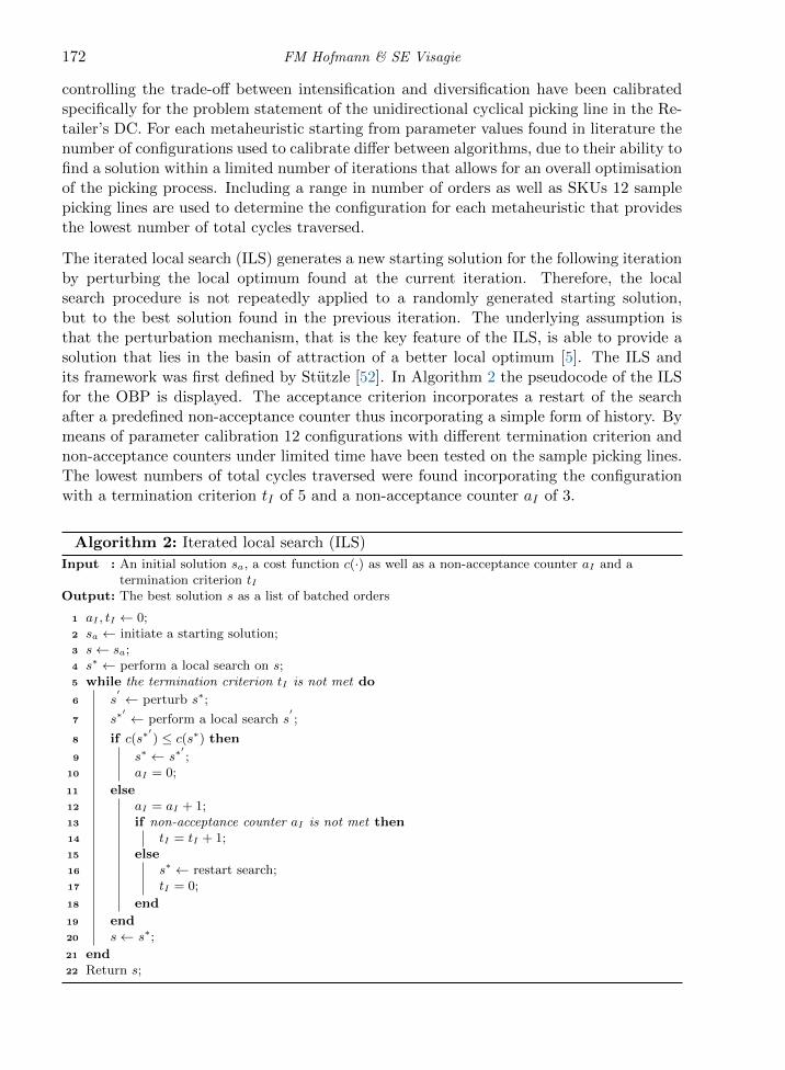
The iterated local search (ILS) generates a new starting solution for the following iterationby perturbing the local optimum found at the current iteration. Therefore, the localsearch procedure is not repeatedly applied to a randomly generated starting solution,but to the best solution found in the previous iteration. The underlying assumption isthat the perturbation mechanism, that is the key feature of the ILS, is able to provide asolution that lies in the basin of attraction of a better local optimum [5]. The ILS andits framework was first defined by Stutzle [52]. In Algorithm 2 the pseudocode of the ILSfor the OBP is displayed. The acceptance criterion incorporates a restart of the searchafter a predefined non-acceptance counter thus incorporating a simple form of history. Bymeans of parameter calibration 12 configurations with different termination criterion andnon-acceptance counters under limited time have been tested on the sample picking lines.The lowest numbers of total cycles traversed were found incorporating the configurationwith a termination criterion tI of 5 and a non-acceptance counter aI of 3.

Algorithm 2: Iterated local search (ILS)

Input : An initial solution sa, a cost function c(·) as well as a non-acceptance counter aI and atermination criterion tI

Output: The best solution s as a list of batched orders

1 aI , tI ← 0;2 sa ← initiate a starting solution;3 s← sa;4 s∗ ← perform a local search on s;5 while the termination criterion tI is not met do

6 s′← perturb s∗;

7 s∗′← perform a local search s

′;

8 if c(s∗′) ≤ c(s∗) then

9 s∗ ← s∗′;

10 aI = 0;

11 else12 aI = aI + 1;13 if non-acceptance counter aI is not met then14 tI = tI + 1;15 else16 s∗ ← restart search;17 tI = 0;

18 end

19 end20 s← s∗;

21 end22 Return s;

Picking location metrics for order batching 173

The variable neighbourhood search (VNS) explores the solution space by dynamicallychanging neighbourhoods around a given solution. After an initial solution is introduced,the main cycle of the VNS consists of the steps shaking, local search and move. In theshaking step a solution s

′is randomly selected in the hth neighbourhood of the current

solution. If the local search produces a better solution s∗′

than s, the solution is updatedand the algorithm stays in the first neighbourhood. Otherwise, the algorithm moves toexplore the next neighbourhood [5]. Mladenovic & Hansen [40] introduced the structureof this algorithm. The pseudocode displayed in Algorithm 3, applies the VNS to theOBP. In this study three neighbourhoods are defined after testing different configurationsin numerical experiments. In the first neighbourhood the order with the highest costaccording to the picking location metric is swapped with the lowest, then the secondhighest and lowest are swapped as well as the third highest and lowest are interchangedrespectively. The termination criterion tV has been set to 5 through parameter calibrationincluding 6 different configurations of termination criterion tested on the sample pickinglines under time restriction.

Algorithm 3: Variable neighbourhood search (VNS)

Input : An initial solution sa, a set of neighbourhood structures H with h = 1, 2, 3, a costfunction c(·) as well as a termination criterion tV

Output: The best solution s as a list of batched orders

1 tV ← 0;2 H ← generate a set of neighbourhood structures with h = 1, 2, 3;3 sa ← initiate a starting solution;4 s← sa;5 while the termination criterion tV is not met do6 h← 1;7 while in one of the defined neighbourhood structures do

8 s′← select a random solution in the hth neighbourhood Hh(s) of s;

9 s∗′← perform a local search on s

′;

10 if c(s∗′) ≤ c(s) then

11 s← s∗′;

12 h = 1;

13 else14 h = h+ 1;15 end

16 end17 tV = tV + 1;

18 end19 Return s;

The variable neighbourhood descent (VND) is a variation of the variable neighbourhoodsearch. The VND is a deterministic version of the VNS excluding the shaking step [53].The search steps of the VND are illustrated in Algorithm 4. The neighbourhood structurestays the same as in the VNS apart from the termination criterion tD that is set to50 through parameter calibration by testing 10 configurations with varying terminationcriterion on the sample picking lines under limited time. The VND is able to find a feasiblesolution faster than the VNS in this study, thus more configurations can be tested.

174 FM Hofmann & SE Visagie

Algorithm 4: Variable neighbourhood descent (VND)

Input : An initial solution sa, a set of neighbourhood structures H with h = 1, 2, 3, a costfunction c(·) as well as a termination criterion tD

Output: The best solution s as a list of batched orders

1 tD ← 0;2 H ← generate a set of neighbourhood structures with h = 1, 2, 3;3 h← 1;4 sa ← initiate a starting solution;5 s← sa;6 while in one of the neighbourhood structures and the termination criterion tD is not met do

7 s′← perform a local search on s in the hth neighbourhood Hh(s);

8 if c(s′) ≤ c(s) then

9 s← s′;

10 h = 1;

11 else12 h = h+ 1;13 end

14 end15 tD = tD + 1;16 Return s;

In a tabu search (TS) the history of the search is used to escape from local optima as wellas to implement an exploitative strategy. A defined number of previously encounteredsolutions is recorded in a tabu list and thus forbidden to be revisited. The list can bedescribed as a short term memory that prevents the algorithm from endless cycling andforces the search to explore different solution spaces. The length of the tabu list thuscontrols the memory of the search process. Glover [21] first introduced the tabu searchalgorithm. The mechanisms of the human memory inspired the main characteristic of thisalgorithm. Its application to the OBP is illustrated in Algorithm 5. The configurationwith its tabu list length l set to 0.8 relative to the size of the problem and its terminationcriterion tT set to 3 provides the lowest number of total cycles traversed when testing 32configurations with different length of tabu lists and termination criterion on the samplepicking lines under time restriction.

Inspiration for the simulated annealing (SA) algorithm comes from the annealing techniqueused by metallurgists. Material is heated up to a high temperature and then lowered downslowly to obtain a well ordered state of minimum energy. Applying this technique, theobjective function of the optimisation problem is minimised similar to the energy of thematerial [5]. The starting solution and the annealing scheme for the temperature decreaseare initiated. At each iteration, a new solution is accepted with a certain probabilitydetermined by the Metropolis criterion [1]. The SA algorithm was introduced by Kirk-patrick et al. [29] and by Cerny [7] independently. In Algorithm 6 the structure of the SAis illustrated. The annealing scheme is crucial to the performance of the algorithm [14].Therefore, three different approaches in determining the annealing scheme have been anal-ysed for this application. A constant lowering of the temperature, dynamically changingthe temperature according to the acceptance of a number of perturbations as well asrestarting to the initial solution after a number of non-acceptances of the new solutionhave been tested. Thereby, re-heating is incorporated in two variations in the second and

Picking location metrics for order batching 175

Algorithm 5: Tabu search (TS)

Input : An initial solution sa, a neighbourhood N (s), a tabu list length l, a cost function c(·) aswell as a termination criterion tT

Output: The best solution s as a list of batched orders

1 tT ← 0;2 TabuList← ∅;3 sa ← initiate a starting solution;4 s← sa;5 while the termination criterion tT is not met do

6 s′← select the best solution in N (s) \ TabuList;

7 if c(s′) ≤ c(s) then

8 s← s′;

9 Update TabuList;10 tT = 0;

11 else12 tT = tT + 1;13 end

14 end15 Return s;

third configuration of the algorithm. Numerical experiments showed that using the accep-tance of a perturbation performs best in the application of this study. Additionally, theparameters initial temperature ta was set to 1.0, the alpha value α to 0.9, the acceptancecounter aS to 12 as well as the termination criterion tS to 3 through fine-tuning initialtemperature, alpha value, acceptance counter and termination criterion in 120 differentconfigurations under limited time.

The great deluge (GD) algorithm is a variation of the SA algorithm. It differs in theacceptance of solutions and is easier to apply, since it only has one parameter that needsto be determined. The metaphor this algorithm uses is that of a hiker that tries to keep herfeet dry while visiting the peaks of an explored area under a slowly rising water level [14].Dueck [15] proposed this algorithm and it is applied to the OBP as illustrated in thepseudocode of Algorithm 7. The parameters have been calibrated to a rain speed r of 0.5as well as a termination criterion tG that is set to 5 with 40 different configurations for rainspeed and termination criterion tested on the sample picking lines under time restriction.

6 Experimental results

The proposed picking location metrics that approximate the distance needed to pick ordersbefore pickers are routed and thus aims at minimising the picking incompatibility betweenorders as well as the algorithms that combine orders in batches on the basis of thesemetrics are tested on 50 sample picking lines. Thereby, the best combinations of metricand algorithm are determined and the best combination to introduce order batching toa unidirectional cyclical picking line is identified. Information about the data set, theexperiment and the statistical analysis of the results are provided in the following sections.

176 FM Hofmann & SE Visagie

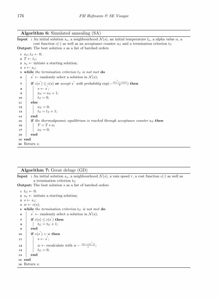
Algorithm 6: Simulated annealing (SA)

Input : An initial solution sa, a neighbourhood N (s), an initial temperature ta, a alpha value α, acost function c(·) as well as an acceptance counter aS and a termination criterion tS

Output: The best solution s as a list of batched orders

1 aS , tS ← 0;2 T ← ta;3 sa ← initiate a starting solution;4 s← sa;5 while the termination criterion tS is not met do

6 s′← randomly select a solution in N (s);

7 if c(s′) ≤ c(s) or accept s

′with probability exp(− c(s

′)−c(s)T

) then

8 s← s′;

9 aS = aS + 1;10 tS = 0;

11 else12 aS = 0;13 tS = tS + 1;

14 end15 if the thermodynamic equilibrium is reached through acceptance counter aS then16 T = T ∗ α;17 aS = 0;

18 end

19 end20 Return s;

Algorithm 7: Great deluge (GD)

Input : An initial solution sa, a neighbourhood N (s), a rain speed r, a cost function c(·) as well asa termination criterion tG

Output: The best solution s as a list of batched orders

1 tG ← 0;2 sa ← initiate a starting solution;3 s← sa;4 w ← c(s);5 while the termination criterion tG is not met do

6 s′← randomly select a solution in N (s);

7 if c(s) ≤ c(s′) then

8 tG = tG + 1;9 end

10 if c(s′) < w then

11 s← s′;

12 w ← recalculate with w − (w−c(s′))

r;

13 tG = 0;

14 end

15 end16 Return s;

Picking location metrics for order batching 177

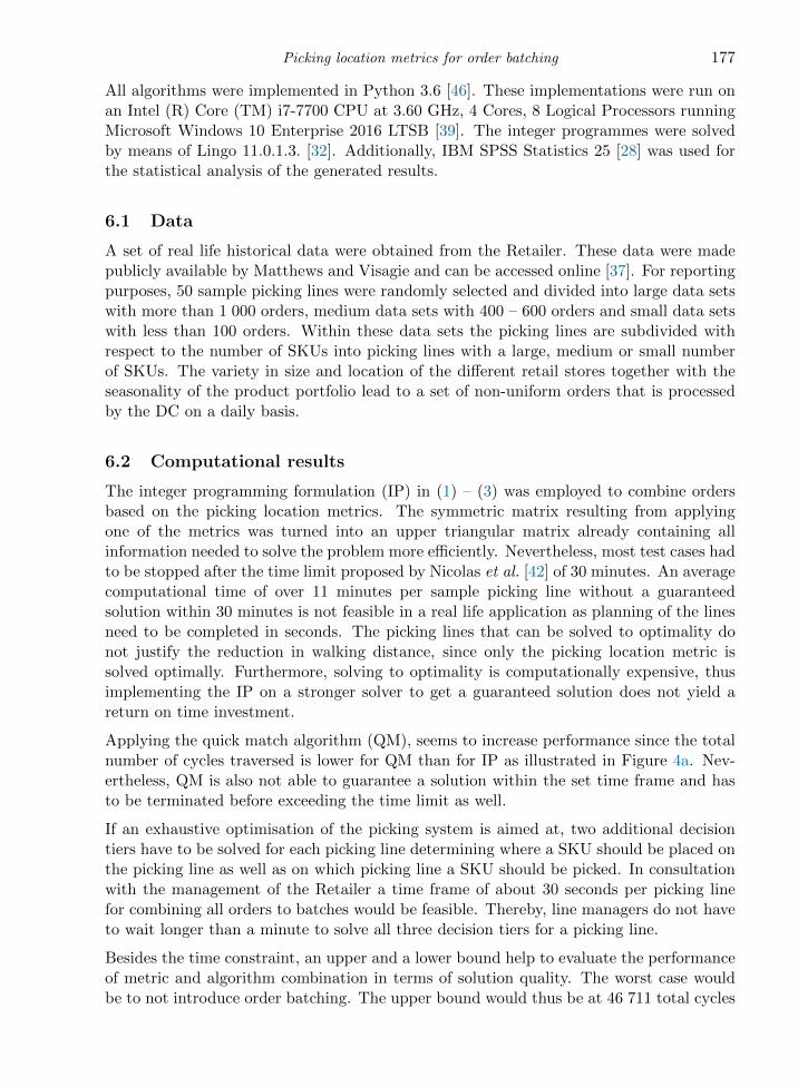
All algorithms were implemented in Python 3.6 [46]. These implementations were run onan Intel (R) Core (TM) i7-7700 CPU at 3.60 GHz, 4 Cores, 8 Logical Processors runningMicrosoft Windows 10 Enterprise 2016 LTSB [39]. The integer programmes were solvedby means of Lingo 11.0.1.3. [32]. Additionally, IBM SPSS Statistics 25 [28] was used forthe statistical analysis of the generated results.

6.1 Data

A set of real life historical data were obtained from the Retailer. These data were madepublicly available by Matthews and Visagie and can be accessed online [37]. For reportingpurposes, 50 sample picking lines were randomly selected and divided into large data setswith more than 1 000 orders, medium data sets with 400 – 600 orders and small data setswith less than 100 orders. Within these data sets the picking lines are subdivided withrespect to the number of SKUs into picking lines with a large, medium or small numberof SKUs. The variety in size and location of the different retail stores together with theseasonality of the product portfolio lead to a set of non-uniform orders that is processedby the DC on a daily basis.

6.2 Computational results

The integer programming formulation (IP) in (1) – (3) was employed to combine ordersbased on the picking location metrics. The symmetric matrix resulting from applyingone of the metrics was turned into an upper triangular matrix already containing allinformation needed to solve the problem more efficiently. Nevertheless, most test cases hadto be stopped after the time limit proposed by Nicolas et al. [42] of 30 minutes. An averagecomputational time of over 11 minutes per sample picking line without a guaranteedsolution within 30 minutes is not feasible in a real life application as planning of the linesneed to be completed in seconds. The picking lines that can be solved to optimality donot justify the reduction in walking distance, since only the picking location metric issolved optimally. Furthermore, solving to optimality is computationally expensive, thusimplementing the IP on a stronger solver to get a guaranteed solution does not yield areturn on time investment.

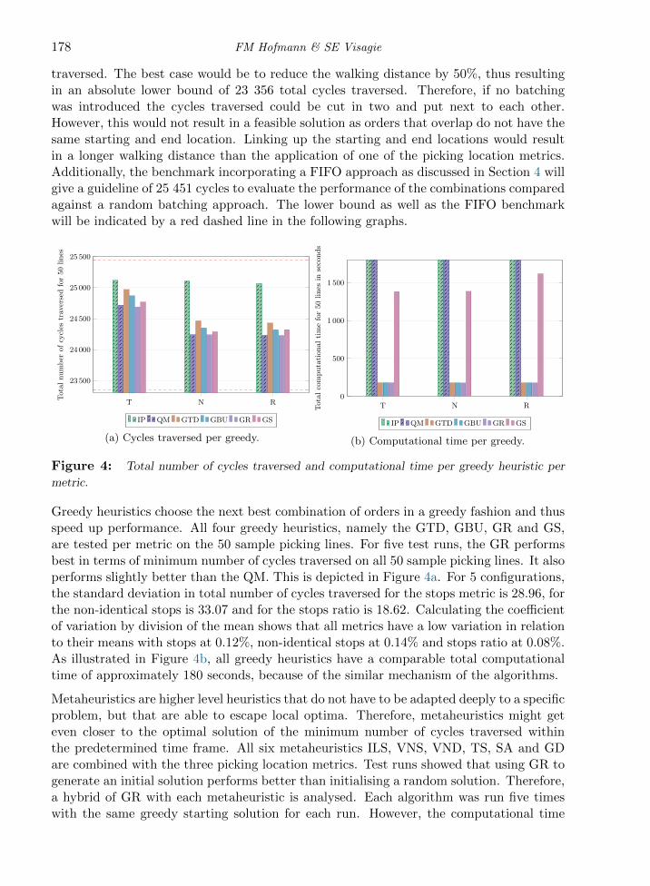
Applying the quick match algorithm (QM), seems to increase performance since the totalnumber of cycles traversed is lower for QM than for IP as illustrated in Figure 4a. Nev-ertheless, QM is also not able to guarantee a solution within the set time frame and hasto be terminated before exceeding the time limit as well.

If an exhaustive optimisation of the picking system is aimed at, two additional decisiontiers have to be solved for each picking line determining where a SKU should be placed onthe picking line as well as on which picking line a SKU should be picked. In consultationwith the management of the Retailer a time frame of about 30 seconds per picking linefor combining all orders to batches would be feasible. Thereby, line managers do not haveto wait longer than a minute to solve all three decision tiers for a picking line.

Besides the time constraint, an upper and a lower bound help to evaluate the performanceof metric and algorithm combination in terms of solution quality. The worst case wouldbe to not introduce order batching. The upper bound would thus be at 46 711 total cycles

178 FM Hofmann & SE Visagie

traversed. The best case would be to reduce the walking distance by 50%, thus resultingin an absolute lower bound of 23 356 total cycles traversed. Therefore, if no batchingwas introduced the cycles traversed could be cut in two and put next to each other.However, this would not result in a feasible solution as orders that overlap do not have thesame starting and end location. Linking up the starting and end locations would resultin a longer walking distance than the application of one of the picking location metrics.Additionally, the benchmark incorporating a FIFO approach as discussed in Section 4 willgive a guideline of 25 451 cycles to evaluate the performance of the combinations comparedagainst a random batching approach. The lower bound as well as the FIFO benchmarkwill be indicated by a red dashed line in the following graphs.

T N R

23 500

24 000

24 500

25 000

25 500

Tota

lnum

ber

of

cycl

estr

aver

sed

for

50

lines

IP QM GTD GBU GR GS

(a) Cycles traversed per greedy.

T N R0

500

1 000

1 500

Tota

lco

mputa

tional

tim

efo

r50

lines

inse

conds

IP QM GTD GBU GR GS

(b) Computational time per greedy.

Figure 4: Total number of cycles traversed and computational time per greedy heuristic per

metric.

Greedy heuristics choose the next best combination of orders in a greedy fashion and thusspeed up performance. All four greedy heuristics, namely the GTD, GBU, GR and GS,are tested per metric on the 50 sample picking lines. For five test runs, the GR performsbest in terms of minimum number of cycles traversed on all 50 sample picking lines. It alsoperforms slightly better than the QM. This is depicted in Figure 4a. For 5 configurations,the standard deviation in total number of cycles traversed for the stops metric is 28.96, forthe non-identical stops is 33.07 and for the stops ratio is 18.62. Calculating the coefficientof variation by division of the mean shows that all metrics have a low variation in relationto their means with stops at 0.12%, non-identical stops at 0.14% and stops ratio at 0.08%.As illustrated in Figure 4b, all greedy heuristics have a comparable total computationaltime of approximately 180 seconds, because of the similar mechanism of the algorithms.

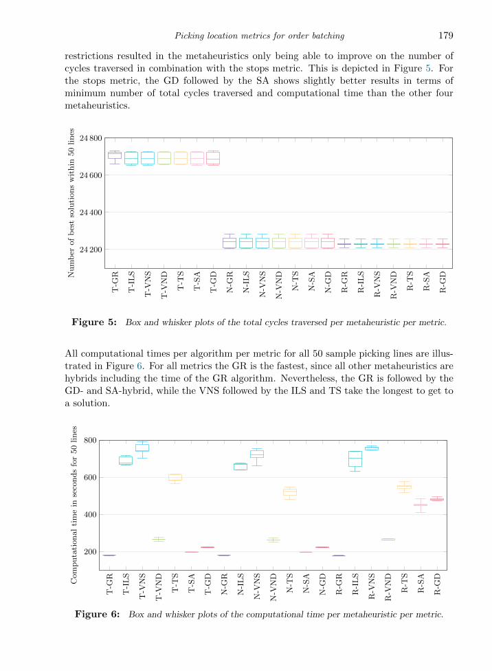
Metaheuristics are higher level heuristics that do not have to be adapted deeply to a specificproblem, but that are able to escape local optima. Therefore, metaheuristics might geteven closer to the optimal solution of the minimum number of cycles traversed withinthe predetermined time frame. All six metaheuristics ILS, VNS, VND, TS, SA and GDare combined with the three picking location metrics. Test runs showed that using GR togenerate an initial solution performs better than initialising a random solution. Therefore,a hybrid of GR with each metaheuristic is analysed. Each algorithm was run five timeswith the same greedy starting solution for each run. However, the computational time

Picking location metrics for order batching 179

restrictions resulted in the metaheuristics only being able to improve on the number ofcycles traversed in combination with the stops metric. This is depicted in Figure 5. Forthe stops metric, the GD followed by the SA shows slightly better results in terms ofminimum number of total cycles traversed and computational time than the other fourmetaheuristics.

T-G

R

T-I

LS

T-V

NS

T-V

ND

T-T

S

T-S

A

T-G

D

N-G

R

N-I

LS

N-V

NS

N-V

ND

N-T

S

N-S

A

N-G

D

R-G

R

R-I

LS

R-V

NS

R-V

ND

R-T

S

R-S

A

R-G

D

24 200

24 400

24 600

24 800

Num

ber

of

bes

tso

luti

ons

wit

hin

50

lines

Figure 5: Box and whisker plots of the total cycles traversed per metaheuristic per metric.

All computational times per algorithm per metric for all 50 sample picking lines are illus-trated in Figure 6. For all metrics the GR is the fastest, since all other metaheuristics arehybrids including the time of the GR algorithm. Nevertheless, the GR is followed by theGD- and SA-hybrid, while the VNS followed by the ILS and TS take the longest to get toa solution.

T-G

R

T-I

LS

T-V

NS

T-V

ND

T-T

S

T-S

A

T-G

D

N-G

R

N-I

LS

N-V

NS

N-V

ND

N-T

S

N-S

A

N-G

D

R-G

R

R-I

LS

R-V

NS

R-V

ND

R-T

S

R-S

A

R-G

D

200

400

600

800

Com

puta

tional

tim

ein

seco

nds

for

50

lines

Figure 6: Box and whisker plots of the computational time per metaheuristic per metric.

180 FM Hofmann & SE Visagie

The hybridisation between metaheuristics may also lead to a better solution quality andan improvement in computational time. Therefore, the combination of metaheuristics hasbeen tested for example picking lines, but has shown no constant improvement under thetime restriction.

Metaheuristics could not improve the solution quality under the time restriction for twoout of three picking location metrics. This raises the question whether the solution foundby GR is close to optimal (and thus few improvements exist) or the metaheuristics areincapable of finding improvements on a poor solution found by the GR. To evaluate thisquestion a sample picking line in which the IP was able to find the optimal solution withinthe time frame is analysed. For the stops metric possible combinations on a sample pickingline with 1 336 orders and 55 SKUs is investigated. The IP is able to generate the bestsolution of 620 cycles that have to be traversed to pick all orders in 137.73 seconds. Whilethe GR algorithms is able to get to 631 cycles in approximately 5 seconds, the GD- aswell as the SA-hybrid are able to reach 629 cycles in almost the same time. The solutionare within 98.55% very close to the best solution. These results indicate that the morecomputational time a metaheuristics is allowed to use, the closer it can get to the bestsolution. However, if the walking distance could be reduced by 50% the lowest boundwould be at 594 cycles. A sample picking line with 1 356 orders and 51 SKUs is analysedfor the non-identical stops metric. It takes 169.72 seconds for the IP to generate thebest solution of 599 cycles that have to be traversed to collect all orders. None of themetaheuristics is able to improve on the GR solution within the given time restrictions.Nevertheless, the GR solution is within 99.50% the best solution for this metric, while thelower bound for this example would be at 573 cycles. For the stops ratio metric a samplepicking line with 1 354 orders and 56 SKUs is investigated. The IP generates the optimalsolution of 583 cycles in 118.91 seconds that have to be traversed. No metaheuristic isable to improve on the GR solution within the predetermined time restriction. However,the solution is within 99.49% also very close to the best solution and the lower bound forthis example is at 555 cycles.

Figure 5 suggests the combination of the stops metric with GR-GD-hybrid, the non-identical stops metric with GR as well as the stops ratio metric with GR, because ofthe minimum number of total cycles traversed generated by these combinations. This issupported by the lowest total computational times for these algorithms as illustrated inFigure 6.

6.3 Statistical analysis

A regression analysis per location metric supports the application of location-based metricsas approximations for walking distance before picker routing. The correlation between theobjective value per metric and the number of cycles traversed is evaluated. This results inR2 = 0.783 for stops, R2 = 0.784 for non-identical stops and R2 = 0.776 for stops ratio.This shows a strong correlation between all metrics and final walking distance. While theapproximation purpose of each metric is validated, the regression analysis does not providea basis for comparison of metrics, since the objective values of all metrics are expressed indifferent units.

Picking location metrics for order batching 181

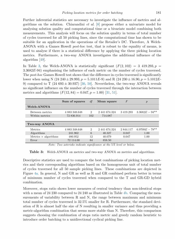
Further inferential statistics are necessary to investigate the influence of metrics and al-gorithms on the solution. Chiarandini et al. [8] propose either a univariate model foranalysing solution quality and computational time or a bivariate model combining bothmeasurements. This analysis will focus on the solution quality in terms of total numberof cycles traversed for all 50 picking lines, since the computational time has shown to besuitable for an application in the operations of the Retailer’s DC. Therefore, A Welch-ANOVA with a Games Howell post-hoc test, that is robust to the equality of means, isused to analyse if there is a statistical difference by applying the three picking locationmetrics. Furthermore, a two-way ANOVA investigates the additional influence of thealgorithm [49].

In Table 3, the Welch-ANOVA is statistically significant (F (2, 102) = 3 419.293, p =3.3682E-94) emphasising the influence of each metric on the number of cycles traversed.The post-hoc Games Howell test shows that the difference in cycles traversed is significantlylower when using N (24 240± 29.993, p = 5.1011E-9) and R (24 230± 16.90, p = 5.1012E-9) compared to T (24 693 ± 30.937) [30, 50]. Nevertheless, the two-way ANOVA revealsno significant influence on the number of cycles traversed through the interaction betweenmetrics and algorithms (F (12, 84) = 0.047, p = 1.00) [31, 51].

Sum of squares df Mean square F p

Welch-ANOVA

Between metrics 4 883 348.648 2 2 441 674.324 3 419.293 3.3682E − 94**Within metrics 72 836.914 102 714.087

Two-way ANOVA

Metrics 4 883 348.648 2 2 441 674.324 2 844.117 6.9709E − 78**Algorithms 241.962 6 40.327 0.047 1.00Metrics × algorithms 480.952 12 40.079 0.047 1.00Error 72 114.00 84 858.50

Note: Two asterisks indicate significance at the 5% level or below.

Table 3: Welch-ANOVA on metrics and two-way ANOVA on metrics and algorithms.

Descriptive statistics are used to compare the best combinations of picking location met-rics and their corresponding algorithms based on the homogeneous unit of total numberof cycles traversed for all 50 sample picking lines. These combinations are depicted inFigure 4a. In general, N and GR as well as R and GR combined perform better in termsof minimum number of cycles traversed when compared to the T and GR-GD hybridcombination.

Moreover, stops ratio shows lower measures of central tendency than non-identical stopswith a mean of 24 230 compared to 24 240 as illustrated in Table 4b. Comparing the mea-surements of variability between R and N, the range between maximum and minimumtotal number of cycles traversed is 32.5% smaller for R. Furthermore, the standard devi-ation of R is almost half the size of N resulting in smaller variance and thus providing ametric-algorithm combination that seems more stable than N. Therefore, this comparisonsuggests choosing the combination of stops ratio metric and greedy random heuristic tointroduce order batching to a unidirectional cyclical picking line.

182 FM Hofmann & SE Visagie

T+GR-GD N+GR R+GR

24 200

24 400

24 600

Num

ber

of

bes

tso

luti

ons

wit

hin

50

lines

(a) Box-whisker plot for each combination.

T+GR-GD N+GR R+GR

Mean 24 693 24 240 24 230Median 24 687 24 243 24 229Range 76 77 52Std.Dev. 30.937 29.993 16.900Variance 957.104 899.558 285.600

(b) Descriptive statistics.

Table 4: Comparison between best combinations of metric and algorithm.

7 Conclusion

In this paper order batching has been introduced to a unidirectional cyclical picking lineas deployed in the layout of a South African retailer’s DC. Three location-based order-to-route closeness metrics have been proposed to approximate the walking distance beforepicker routing and thus identify compatible orders. The picking location metrics includestops counting all locations a picker has to stop and pick for an order, non-identical stopscounting the locations a picker has to stop to pick for only one order and stops ratio de-scribing the ratio between non-identical and combined stops. The assignment problem ofgrouping orders in batches of size two has been solved with exact, greedy and metaheuris-tic solution approaches. The exact solution approaches take too much computational timeto allow for an integrated optimisation approach. Therefore, four greedy heuristics in-cluding a top-down, bottom-up, random and smallest entry search approach as well as sixmetaheuristics namely an iterated local search, a variable neighbourhood search, a variableneighbourhood descent, a tabu search, a simulated annealing and a great deluge algorithmhave been applied to 50 sample picking lines. The picking lines have been recorded fromreal life data and vary in size by number of orders and SKUs. The algorithms terminateafter a reasonable computational time restriction to allow for a real life application. Allmetrics and algorithms have been tested in different combinations to identify the bestcombinations reducing the total number of cycles traversed. This results in the best com-binations of stops and greedy random-great deluge, non-identical stops and greedy randomas well as stops ratio and greedy random.

These best combinations are then compared in terms of minimum number of cycles tra-versed for all 50 picking lines. The stops ratio and greedy combination shows the lowestaverage of 24 230 cycles within the five test runs. Therefore, this combination is recom-mended to be applied if order batching is introduced to a unidirectional cyclical pickingline. Compared to the FIFO benchmark of 25 451 cycles through applying random batch-ing, this is 4.80% less walking distance. If batching is not introduced to the unidirectionalcyclical picking line using this combination, pickers have to walk approximately 48.13%further. Additionally, this combination is only 3.74% higher than the absolute lower bound

Picking location metrics for order batching 183

of reducing 50% of the walking distance. The reduction in walking distance through thecombination of stops ratio and greedy random heuristic can be translated into time savingsleading to a direct decrease of picking cost.

The analysis of the generated results indicate two findings. Firstly, the metric appliedplays a more important role than the algorithm used to group the orders into batches.Secondly, the more information about the location of the items of an order is available,the better the results in terms of minimum number of cycles traversed. Therefore, futurework should incorporate more information in the metric about the specific layout of aunidirectional cyclical picking. This could help to find an even better approximation ofwalking distance and thus get even closer to the lower bound of saving 50% of walkingdistance by picking two orders at a time.

References

[1] Aarts E & Korst J, 1988, Simulated annealing and Boltzmann machines, John Wiley and SonsInc., New York.

[2] Albareda-Sambola M, Alonso-Ayuso A, Molina E & De Blas CS, 2009, Variable neighborhoodsearch for order batching in a warehouse, Asia-Pacific Journal of Operational Research, 26(05),pp. 655–683.

[3] Bartholdi JJ & Hackman ST, 2016, Warehouse & Distribution Science: Release 0.97, SupplyChain and Logistics Institute, Available from https://www.warehouse-science.com/book/index.

html.

[4] Blum C & Roli A, 2003, Metaheuristics in combinatorial optimization: Overview and conceptualcomparison, ACM computing surveys (CSUR), 35(3), pp. 268–308.

[5] BoussaıD I, Lepagnot J & Siarry P, 2013, A survey on optimization metaheuristics, InformationSciences, 237, pp. 82–117.

[6] Bozer YA & Kile JW, 2008, Order batching in walk-and-pick order picking systems, InternationalJournal of Production Research, 46(7), pp. 1887–1909.

[7] Cerny V, 1985, Thermodynamical approach to the traveling salesman problem: An efficient simula-tion algorithm, Journal of optimization theory and applications, 45(1), pp. 41–51.

[8] Chiarandini M, Paquete L, Preuss M & Ridge E, 2007, Experiments on metaheuristics:Methodological overview and open issues, Technical Report DMF-2007-03-003, Available from https:

//pdfs.semanticscholar.org/9fcd/f48d4ae1770a6c653e33caee25aeb109b44d.pdf.

[9] Clarke G & Wright JW, 1964, Scheduling of vehicles from a central depot to a number of deliverypoints, Operations research, 12(4), pp. 568–581.

[10] Dallari F, Marchet G & Melacini M, 2009, Design of order picking system, The InternationalJournal of Advanced Manufacturing Technology, 42(1), pp. 1–12.

[11] De Koster M, Van der Poort ES & Wolters M, 1999, Efficient orderbatching methods inwarehouses, International Journal of Production Research, 37(7), pp. 1479–1504.

[12] De Koster R, Le-Duc T & Roodbergen KJ, 2007, Design and control of warehouse order picking:A literature review, European Journal of Operational Research, 182(2), pp. 481–501.

[13] De Villiers AP, 2012, Minimising the total travel distance to pick orders on a unidirectional pickingline.

184 FM Hofmann & SE Visagie

[14] Dreo J, Petrowski A, Siarry P & Taillard E, 2006, Metaheuristics for hard optimization:methods and case studies, Springer Science & Business Media, Berlin.

[15] Dueck G, 1993, New optimization heuristics, Journal of Computational physics, 104(1), pp. 86–92.

[16] Elsayed EA & Stern RG, 1983, Computerized algorithms for order processing in automated ware-housing systems, The International Journal of Production Research, 21(4), pp. 579–586.

[17] Elsayed EA & Unal O, 1989, Order batching algorithms and travel-time estimation for automatedstorage/retrieval systems, The International Journal of Production Research, 27(7), pp. 1097–1114.

[18] Frazelle E, 2002, World-class warehousing and material handling, volume 1, McGraw-Hill NewYork.

[19] Gademann N & Velde S, 2005, Order batching to minimize total travel time in a parallel-aislewarehouse, Institute of Industrial Engineers Transactions, 37(1), pp. 63–75.

[20] Gibson DR & Sharp GP, 1992, Order batching procedures, European Journal of Operational Re-search, 58(1), pp. 57–67.

[21] Glover F, 1986, Future paths for integer programming and links to artificial intelligence, Computers& operations research, 13(5), pp. 533–549.

[22] Gu J, Goetschalckx M & McGinnis LF, 2007, Research on warehouse operation: A comprehensivereview, European Journal of Operational Research, 177(1), pp. 1–21.

[23] Henn S, Koch S, Doerner KF, Strauss C & Wascher G, 2010, Metaheuristics for the orderbatching problem in manual order picking systems, Business Research, 3(1), pp. 82–105.

[24] Henn S, Koch S & Wascher G, 2012, Order batching in order picking warehouses: a survey ofsolution approaches, pp. 105–137 in Warehousing in the Global Supply Chain, pp. 105–137. Springer,London.

[25] Henn S & Wascher G, 2012, Tabu search heuristics for the order batching problem in manual orderpicking systems, European Journal of Operational Research, 222(3), pp. 484–494.

[26] Ho YC, Su TS & Shi ZB, 2008, Order-batching methods for an order-picking warehouse with twocross aisles, Computers & Industrial Engineering, 55(2), pp. 321–347.

[27] Ho YC & Tseng YY, 2006, A study on order-batching methods of order-picking in a distributioncentre with two cross-aisles, International Journal of Production Research, 44(17), pp. 3391–3417.

[28] IBM, 2018, Spss version 25, [Online], [Cited October 8th, 2018], Available from https://www.ibm.

com/analytics/spss-statistics-software.

[29] Kirkpatrick S, Gelatt CD & Vecchi MP, 1983, Optimization by simulated annealing, science,220(4598), pp. 671–680.

[30] Laerd Statistics, 2018, One-way anova in spss statistics (cont), [Online], [CitedOctober 5th, 2018], Available from https://statistics.laerd.com/spss-tutorials/

one-way-anova-using-spss-statistics-2.php.

[31] Laerd Statistics, 2018, Two-way anova in spss statistics (cont), [Online], [CitedOctober 5th, 2018], Available from https://statistics.laerd.com/spss-tutorials/

two-way-anova-using-spss-statistics-2.php.

[32] Lindo Systems, 2018, Lingo 11, [Online], [Cited October 8th, 2018], Available from https://www.

lindo.com/.

[33] Litvak N & Vlasiou M, 2010, A survey on performance analysis of warehouse carousel systems,Statistica Neerlandica, 64(4), pp. 401–447.

Picking location metrics for order batching 185

[34] Matthews J, 2012, Order sequencing and SKU arrangement on a unidirectional picking line.

[35] Matthews J, 2015, Sku assignment in a multiple picking line order picking system., Doctoral Dis-sertation, Stellenbosch: Stellenbosch University.

[36] Matthews J & Visagie SE, 2013, Order sequencing on a unidirectional cyclical picking line, Euro-pean Journal of Operational Research, 231(1), pp. 79–87.

[37] Matthews J & Visagie SE, 2014, Picking line data set a, [Online], [Cited October 5th, 2018],Available from http://hdl.handle.net/10019.1/86143.

[38] Matusiak M, de Koster R, Kroon L & Saarinen J, 2014, A fast simulated annealing method forbatching precedence-constrained customer orders in a warehouse, European Journal of OperationalResearch, 236(3), pp. 968–977.

[39] Microsoft, 2018, [Cited October 8th, 2018], Available from https://www.microsoft.com/.

[40] Mladenovic N & Hansen P, 1997, Variable neighborhood search, Computers & operations research,24(11), pp. 1097–1100.

[41] Muter I & Oncan T, 2015, An exact solution approach for the order batching problem, IIE Trans-actions, 47(7), pp. 728–738.

[42] Nicolas L, Yannick F & Ramzi H, 2017, Optimization of order batching in a picking system withcarousels, IFAC-PapersOnLine, 50(1), pp. 1106–1113.

[43] Oncan T, 2015, Milp formulations and an iterated local search algorithm with tabu thresholding forthe order batching problem, European Journal of Operational Research, 243(1), pp. 142–155.

[44] Orlin JB & Lee Y, 1993, Quickmatch–a very fast algorithm for the assignment problem, Alfred P.Sloan School of Management.

[45] Pan CH & Liu S, 1995, A comparative study of order batching algorithms, Omega, 23(6), pp. 691–700.

[46] Python Software Foundation, 2018, Python 3.6, [Online], [Cited October 8th, 2018], Availablefrom https://www.python.org/.

[47] Rosenwein M, 1996, A comparison of heuristics for the problem of batching orders for warehouseselection, International Journal of Production Research, 34(3), pp. 657–664.

[48] Rouwenhorst B, Reuter B, Stockrahm V, van Houtum GJ, Mantel R & Zijm W, 2000,Warehouse design and control: Framework and literature review, European Journal of OperationalResearch, 122(3), pp. 515–533.

[49] Sheskin DJ, 2000, Handbook of parametric and nonparametric statistical procedures, CRC Press,Florida, United States.

[50] SPSS Tutorials, 2018, Spss one-way anova tutorial, [Online], [Cited October 5th, 2018], Availablefrom https://www.spss-tutorials.com/spss-one-way-anova/.

[51] SPSS Tutorials, 2018, Spss two way anova – basics tutorial, [Online], [Cited October 5th, 2018],Available from https://www.spss-tutorials.com/spss-two-way-anova-basics-tutorial/.

[52] Stutzle T, 1998, Local search algorithms for combinatorial problems, Doctoral Dissertation, Darm-stadt University of Technology.

[53] Talbi EG, 2009, Metaheuristics: from design to implementation, John Wiley & Sons, New Jersey,United States.

186 FM Hofmann & SE Visagie

[54] Van den Berg JP & Zijm WH, 1999, Models for warehouse management: Classification and ex-amples, International Journal of Production Economics, 59(1-3), pp. 519–528.

[55] Wascher G, 2004, Order picking: a survey of planning problems and methods, pp. 323–347 in Supplychain management and reverse logistics, pp. 323–347. Springer, Heidelberg.

[56] Zulj I, Kramer S & Schneider M, 2018, A hybrid of adaptive large neighborhood search and tabusearch for the order-batching problem, European Journal of Operational Research, 264(2), pp. 653–664.