Embed Size (px)
Citation preview
PHZ 7427 SOLID STATE II:
Electron-electron interaction and the Fermi-liquid theory
D. L. Maslov
Department of Physics, University of Florida
(Dated: February 21, 2014)
1
CONTENTS
I.Notations 2
II.Electrostatic screening 2
A.Thomas-Fermi model 2
B.Effective strength of the electron-electron interaction. Parameter rs. 2
C.Full solution (Lindhard function) 3
D.Lindhard function 5
1.A discourse: properties of Fourier transforms 6
2.End of discourse 7
E.Friedel oscillations 7
1.Enhancement of the backscattering probability due to Friedel oscillations 8
F.Hamiltonian of the jellium model 9
G.Effective mass near the Fermi level 13
1.Effective mass in the Hartree-Fock approximation 15
2.Beyond the Hartree-Fock approximation 15
III.Stoner model of ferromagnetism in itinerant systems 16
IV.Wigner crystal 20
V.Fermi-liquid theory 22
A.General concepts 22
1.Motivation 23
B.Scattering rate in an interacting Fermi system 24
C.Quasi-particles 27
1.Interaction of quasi-particles 29
D.General strategy of the Fermi-liquid theory 31
E.Effective mass 31
F.Spin susceptibility 33
1.Free electrons 33
2.Fermi liquid 34
G.Zero sound 35
2
VI.Non- Fermi-liquid behaviors 37
A.Dirty Fermi liquids 38
1.Scattering rate 38
2.T-dependence of the resistivity 40
A.Born approximation for the Landau function 43
References 44
I. NOTATIONS
• kB = 1 (replace T by kBT in the final results)
• ~ = 1 (momenta and wave numbers have the same units, so do frequency and energy)
• ν(ε) ≡ density of states
II. ELECTROSTATIC SCREENING
A. Thomas-Fermi model
For Thomas-Fermi model, see AM, Ch. 17.
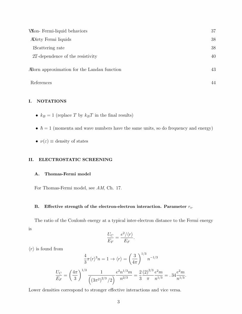
B. Effective strength of the electron-electron interaction. Parameter rs.
The ratio of the Coulomb energy at a typical inter-electron distance to the Fermi energy
isUCEF
=e2/〈r〉EF
.
〈r〉 is found from
4
3π〈r〉3n = 1→ 〈r〉 =
(3
4π
)1/3
n−1/3
UCEF
=
(4π
3
)1/31(
(3π2)2/3 /2) e2n1/3m
n2/3=
2
3
(2)2/3
π
e2m
n1/3= . 34
e2m
n1/3.
Lower densities correspond to stronger effective interactions and vice versa.
3
Parameter rs is introduced as the average distance between electrons measured in units
of the Bohr radius
〈r〉 = rsaB = rs/me2.
Expressing rs in terms of n and relating density to kF , we find
rs =
(3
4π
)1/31
n1/3aB=
(9π
4
)1/3me2
kF.
In terms of rs,
UC =e2
rsaB
and
EF =1
2
(9π
4
)2/31
ma2B
1
r2s
.
UCEF
= 2
(4
9π
)2/3
rs ≈ . 54rs.
C. Full solution (Lindhard function)
In the Thomas-Fermi model, one makes two assumptions: a) the effective potential acting
on electrons is weak and b) the effective potential (and corresponding density) varies slowly
on the scale of the electron’s wavelength. Assumption a) allows one to use the perturbation
theory whereas assumption b) casts this theory into a quasi-classical form. In a full theory,
one discards assumption b) but still keeps assumption a). So now we want to do a complete
quantum-mechanical (no quasi-classical assumptions) form.
Let the total electrostatic potential acting on an electron be
φ = φext + φind,
where φext is the potential of external charges and φind is that of induced charges. Corre-
spondingly, the potential energy
v = −eφ = −eφext − eφind.
Because we are doing the linear-response theory, the form of the external perturbation does
not matter. Let’s choose it as a plane-wave
v (~r, t) =1
2vqe
i(~q·~r−ωt) + c.c. (1)
4
Before the perturbation was applied, the wavefunction was
Ψ0 =1
L3/2e(ik·~r−εkt).
The wavefunction in the presence of the perturbation is given by standard expression from
the first-order perturbation theory
Ψ = Ψ0
[1 +
vq2
ei(~q·~r−ωt)
εk − εk+~q + ω+vq2
e−i(~q·~r−ωt)
εk − εk−~q − ω
],
where the last term is a response to a c.c. term in Eq.(1). The Fourier component of the
wavefunction
Ψk = Ψ0k
[1 +
1
2
vqεk − εk+~q + ω
+1
2
vqεk − εk−~q − ω
].
The induced charge density is related to the wavefunction is
ρind = −2e∑k
fk(|Ψk|2 − |Ψ0k|2
), (2)
where fk is the Fermi function, factor of 2 is from the spin summation and the homogeneous
(unperturbed) charge density was subtracted off. Keeping only the first-order terms in vq,
Eq.(2) gives
ρind = −2e1
L3
∑k
fkvq
[1
εk − εk+~q + ω+
1
εk − εk−~q − ω
](3)
= −2evq
∫d3k
(2π)3
fk − fk+~q
εk − εk+~q + ω, (4)
where we shifted the variables as k− ~q → k and k→ k + q in the last term.
The charge susceptibility, χ, is defined as
ρind = eq2
4πχvq = −e2 q
2
4πχφq, (5)
where φq is the Fourier component of the net electrostatic potential. Comparing Eqs. (4)
and (5), we see that
χ =4π
q2(−2)
∫d3k
(2π)3
fk − fk+~q
εk − εk+~q + ω.
The meaning of χ becomes more clear, if we write down the Poisson equation (in a Fourier-
transformed form)
q2φq = 4π (ρext + ρind) .
5
External charges and potentials satisfy a Poisson equation on their own
q2φext = 4πρext.
Now,
q2φq = q2φext + 4πρind = q2φext − 4πe2 q2
4πχφq →
φq =φext
1 + χe2.
Using a definition of the dielectric function
φq =φext
ε (q, ω), (6)
we see that
ε (q, ω) = 1 + χe2 = 1 +4πe2
q2(−2)
∫d3k
(2π)3
fk − fk+~q
εk − εk+~q + ω. (7)
This is the Lindhard’s expression for the dielectric function.
a. Check Let’s make sure that the general form of ε (q, ω) [Eq.(7)] does reduce to the
Thomas-Fermi one in the limit ω = 0 and q kF .
ε (q, 0) = 1 +4πe2
q2(−2)
∫d3k
(2π)3
fk − fk+~q
εk − εk+~q
For small q,
fk+~q = f (εk+~q) = f (εk+~q − εk + εk)
= f (εk) +∂f
∂εk(εk+~q − εk) + . . .
and
ε (q, 0) = 1 +4πe2
q22
∫d3k
(2π)3
(− ∂f∂εk
).
At T = 0, − ∂f∂εk
= δ (εk − EF ) . The density of states at the Fermi energy
νF = 2
∫d3k
(2π)3 δ (εk − EF ) .
Now,
ε (q, 0) = 1 +4πe2
q2νF = 1 +
κ2
q2,
where κ2 ≡ 4πe2νF , which is just the Thomas-Fermi form.
6
D. Lindhard function
As shown in AM, the static form of the Lindhard’s dielectric function is given by
ε (q, 0) = 1 +4πe2
q2
[1
2+
1− x2
4xln
1 + x
|1− x|
],
where x ≡ q/2kF .
Notice that the derivative of ε (q, 0) is singular for q = 2kF , i.e., x = 1. This singularity
gives rise to a very interesting phenomenon–Friedel oscillations in the induced charge density
(and corresponding potentials). Mathematically, it arises because of the property of the
Fourier transform. To find the net electrostatic potential in the real space we need to
Fourier transform back to real space Eq.(6). Let’s say that the external perturbation is a
single point charge Q. Then (in the q− space) , φext = 4πQ/q2 and
φ (r) =
∫d3q
(2π)3 e−i~q·~r 4πQ
q2ε (q, 0) .(8)
1. A discourse: properties of Fourier transforms
Fourier transforms have the following property. Suppose we want to find the large t limit
of
F (t) =
∫dω
2πe−iωtF (ω) . (9)
If function F (ω) is analytic, the integral in Eq.(6) can be done by closing the contour
in the complex plane. F (t) for t → ∞ will be then given by an exponentially decaying
function exp(−ω′′mint) , where ω′′min is the imaginary part of that pole of F (ω) which is
closest to the real axis. For example, if F (ω) = (ω2 + a2)−1, F (t) ∝ exp (−at) . Thus, the
large-t asymptotes of analytic functions decay exponentially in time. On the other hand,
if F (ω) is non-analytic, F (t) decays much slower–only as a power-law. For example, for
F (ω) = exp (−a |ω|) , we have
F (t) =
∫dω
2πe−iωt exp (−a |ω|) =
∫ ∞0
dω
2π
(e−iωt + eiωt
)e−aω
= 2Re
∫ ∞0
dω
2πe−iωte−aω = 2Re
1
2π
1
a+ it=
1
π
a
a2 + t2∝ 1
t2for t→∞.
In addition, if F (ω) has a divergent derivative of order n at finite ω, e.g., for ω = ω0, that
F (t) oscillates in t. This can be seen by doing the partial integration in Eq.(6) n+ 1 times
2πF (t) =
∫dωe−iωtF (ω) =
∫ ω0
−∞dωe−iωtF (ω) +
∫ ∞ω0
dωe−iωtF (ω) =
7
=1
−iωe−iωtF (ω) |ω0
−∞ +1
−iωe−iωtF (ω) |∞ω0
−(
1
−iω
)∫dωe−iωt
d
dωF (ω) + . . . ,
i.e., until the boundary terms gives the divergent expression dn
dωnF (ω0) e−iω0t which oscillates
as e−iω0t.
2. End of discourse
Coming back to Eq.(9), we can now understand why the induced density around the
point charge oscillates as cos 2kF r and falls off only as a power law of the distance
ρind ∝cos 2kF r
r3.
Both of these effects are the consequences of the singularity of ε (q, 0) at q = 2kF .
E. Friedel oscillations
The physics of Friedel oscillations is very simple: they arise due to standing waves formed
as a result of interference between incoming and backscattered electron waves. For the sake
of simplicity, let’s analyze a 1D case. Suppose that at x = 0, we have an infinitely high
barrier (wall). For each k, the wavefunction is a superposition of the incoming plane wave
L−1/2eikx and a reflected wave L−1/2e−ikx :
Ψ = L−1/2eikx − L−1/2e−ikx =2i
L1/2sin kx
The probability density |Ψ|2 = (4/L) sin2 kx oscillates in space. If the probability that the
state with momentum k is occupied is a smooth function of k (as it is the case for the
Maxwell-Boltzmann or Bose-Einstein statistics), then summation over k would smear out
the oscillations. However, for the Fermi statistics, fk has a sharp (at T = 0) boundary
between the occupied and empty states. As a result, oscillations survive even after the
summation of k. The profile of the density is described by
n (x) = 2∑k
dk
2πfk |Ψ|2 = 8
∫ kF
0
dk
2πsin2 kx = 4
∫ kF
0
dk
2π(1− cos 2kx)
= n0 −sin 2kFx
πx,
where n0 = 2kF/π is the density of the homogeneous electron gas. Away from the barrier,
oscillations die off as x−1. At the barrier, n (0) = 0.
8
A 3D case, is different in that the x−1 decay changes to a r−3 one. (In general D-
dimensional case, the Friedel oscillations fall off as r−D.) Friedel oscillations were observed
in STM experiment (see attached figures).
1. Enhancement of the backscattering probability due to Friedel oscillations
As it was discussed in the previous Section, Friedel oscillations arise already in the single-
particle picture. However, they influence scattering of interacting electrons at impurities and
other imperfections. Once a Friedel oscillation is formed, the effective potential barrier seen
by other electrons is the sum of the bare potential plus the potential produced by the Friedel
oscillation. Consider a simple example when 1D electrons interact via a contact potential
U (x) = uδ (x) . The potential produced by the Friedel oscillation is
VF (x) =
∫dx′ (n (x′)− n0)V (x− x′)
= u (n (x)− n0) = −usin 2kFx
πx.
Backscattering at an oscillatory potential is enhanced due to resonance. In the Born ap-
proximation, the backscattering amplitude for an electron with momentum k is
A =
∫dx(e−ikx
)∗VF (x) eikx = −u
π
∫ ∞0
dx
xsin 2kFxe
i2kx
= −uπ
∫ ∞0
dx
x
(e2i(k+kF )x + e2i(k−kF )x
).
The first term gives a convergent integral (we remind that our k > 0), so forget about it.
(It’s only role is to guarantee the convergence at x→ 0, but we will take this into account by
cutting the integral at x ' k−1F. .)The second term becomes log-divergent at large distances
if k = kF . To estimate the integral, notice that it diverges for k = kF and converges for
k 6= kF . Thus
A = −uπ
∫ |k−kF |−1
k−1F
dx
x= −u
πln
kF|k − kF |
.
Precisely at the Fermi surface (k = kF ), the backscattering amplitude (and thus the prob-
ability) blows up which means that impurity becomes impenetrable. This effect in 1D is
usually described as arising due to the non-Fermi-liquid nature of the ground state? . How-
ever, as we just saw that this effect can be simply understood in terms of backscattering
from the Friedel oscillations1. Higher orders in the e-e interaction can be summed up (see
9
Ref.1). It turns out that each next order in u brings in an additional log of |k − kF | . The
transmission amplitude of the barrier becomes
t = t0
(1− g ln
kF|k − kF |
+1
2g2 ln2 kF
|k − kF |− 1
6g3 ln3 kF
|k − kF |+ . . .
)= t0 exp
(−g ln
kF|k − kF |
)= t0
(|k − kF |kF
)g,
where g = u/πvF is the dimensionless coupling constant and t0 is the transmission amplitude
in the absence of e−e interaction. At k = kF , the transmission amplitude vanishes. Suppose
one measures a tunneling conductance of the barrier inserted into a 1D system. Then
typical |k − kF | ' max T/vF , eV/vF, where V is the applied voltage. With the help of the
Landauer formula G = (2e2/h) |t0|2 we conclude that the tunneling conductance exhibits a
power-law scaling in the voltage or temperature
G ∝ (max T, eV )2g .
Such a power-law scaling was indeed observed in carbon nanotubes (which are essentially
quantum wires with two channels)
F. Hamiltonian of the jellium model
The model system we study are electrons in the presence of a positively charged ions. The
ionic charge is assumed to be spread uniformly over the system volume (“jellium model”).
The net electron charge is equal in magnitude and opposite in sign to the that of ions
so that overall the system is electro-neutral. This part of the model is common for all
tractable models of e-e interactions in solids, including but not limited to the Hartree-Fock
approximation. The classical energy of the system electrons + ions is
Eint =1
2
∫d3r1
∫d3r2n (~r1)Vee (~r1 − ~r2)n (~r2) +
∫d3r1
∫d3r2n (~r1)Vei (~r1 − ~r2)ni(10)
+1
2
∫d3r1
∫d3r2niVii (~r1 − ~r2)ni,
where n (~r) is the (non-uniform) electron density, ni is the (uniform) density of ions, Vee,ei,ii
are the potentials of electron-electron, electron-ion, and ion-ion interactions. In the Hartree-
Fock approximation,
Vee (~r1 − ~r2) =e2
|~r1 − ~r2|= −Vei (~r1 − ~r2) = Vii (~r1 − ~r2) . (11)
10
Using (11), Eq.(12) can be re-arranged as
Eint =1
2
∫d3r1
∫d3r2 [n (~r1)− ni]Vee (~r1 − ~r2) [n (~r2)− ni] .
In this form, the energy has a very simple meaning. At point ~r1 the electron density deviates
from the ionic density, so that the net charge density is n (~r1)−ni. Similarly, at point ~r2 the
net charge density is n (~r2)−ni. These local fluctuations in density interact via the Coulomb
potential. In the absence of any external perturbations, boundaries, and impurities, the
average electron density is uniform and equal to the density of ions: 〈n (~r1)〉 = ni. However,
the ground state energy involves the product of densities at different points 〈n (~r1)n (~r2)〉
(a correlation function) which is not uniform. In classical systems, local fluctuations in the
charge density are due to thermal motion of electrons. In a quantum-mechanical system at
T = 0 they are due to the zero-point motion of electrons (in a Fermi system, the kinetic
energy is finite at T = 0). To treat the QM system, we need to pass from the classical energy
to a Hamiltonian
Eint → Hint =1
2
∫d3r1
∫d3r2 [n (~r1)− ni]Vee (~r1 − ~r2) [n (~r2)− ni] , (12)
where now n (~r) is a number-density operator. Densities of ions do not fluctuate so we can
leave them as classical variables (c-numbers). Also, the potential is the same as in the
classical system. It is convenient to re-write Eq. (12) in a Fourier-transformed form
Hint =1
2
1
L3
∑~q
[n− ni]~q Vee (q) [n− ni]−~q ,
where
n (~r)− ni =1
L3
∑~q
[n (~r)− ni]~q e−i~q·~r
Vee (~r) =1
L3
∑~q
Vee (q) e−i~q·~r,
with Vee (q) = 4πe2/q2 and where we took into account that Vee (q) depends only on the
magnitude of q. The Fourier transform of a uniform density of ions is niL3δ~q,0 so
Hint =1
2
1
L3
∑~q
[n~q − niL3δ~q,0
]Vee (q)
[n−~q − niL3δ~q,0
]=
1
2
1
L3
∑~q
[n~q −Nδ~q,0]Vee (q) [n−~q −Nδ~q,0] ,
11
where N is the total number of ions (equal to that of electrons). On the other hand,
n~q=0 =
∫d3rn (~r) = N ,
where N is an operator of the total number of particles. Because the total number of particles
is fixed this operator is simply equal to its expectation value–N. Thus the ~q = 0 term gives
no contribution to the sum. Physically, it means that the fluctuation of infinite size in real
space (corresponding to ~q = 0) do not interact as they are compensated by uniform charge
of ions. With that, we re-write Hint as
Hint =1
2
1
L3
∑~q 6=0
n~qVee (q) n−~q. (13)
At T = 0, the ground-state energy is simply an expectation value of Hint :
Eint = 〈0∣∣∣Hint
∣∣∣ 0〉 =1
2
1
L3
∑~q 6=0
Vee (q) 〈0 |n~qn−~q| 0〉.
As we simply do the perturbation theory with respect to Vee, the expectation value is cal-
culated using the wave-functions of the free system (vacuum average).
Now we need the second quantized from of n~q. To this end, we recall that in real space
n (~r) =∑α
Ψ†α (~r) Ψα (~r) .
Operator Ψ†α (~r) (Ψα (~r)) creates (annihilates) a particle with spin projection α at point ~r.
Using the plane waves as our basis set,
Ψα (~r) =1
L3/2
∑p
cpαe−ip·~r
Ψ†α (~r) =1
L3/2
∑p
c†pαeip·~r.
n~q =
∫d3rei~q·~rn (~r) =
∫d3rei~q·~r
∑α
Ψ†α (~r) Ψα (~r)
=1
L3
∫d3rei~q·~r
∑α
∑p,p′
c†p′αeip′·~rcpαe
−ip·~r
=∑α
∑p
c†p−~q,αc~pα.
12
Substituting this last result into Eq.(13), we obtain
Hint =1
2
1
L3
∑~q 6=0
∑p,k
∑α,β
Vee (q) c†p−~q,αcpαc†k+~q,βckβ.
It is convenient to re-write the second-quantized Hamiltonians in the normal-ordered form,
when all creation operators are positioned to the right of the annihilation ones. Interchanging
the positions of two fermionic operators twice (no sign change!) and discarding the terms
which result from the δ-function part of the anti-commutation relations (those will give only
a shift of the chemical potential), we arrive at
Hint =1
2
1
L3
∑~q 6=0
∑p,k
∑α,β
Vee (q) c†p−~q,αc†k+~q,βckβcpα.
Thus,
Eint = 〈0∣∣∣Hint
∣∣∣ 0〉 =1
2
1
L3
∑~q 6=0
∑p,k
∑α,β
Vee (q) 〈0∣∣∣c†p−~q,αc†k+~q,βckβcpα
∣∣∣ 0〉.The expectation value of the product of c− operators can be calculated directly. However,
it is much more convenient to use the result known as the Wick’s theorem2,3. The Wick
theorem states that an expectation value of a product of any number of c− operators splits
into products of expectation values of pairwise averages (called contractions):
〈0∣∣ΠM1
i=1c†pi,αi
ΠM2j=1cpj ,αj
∣∣ 0〉 =∑P
ΠM1†i=1pi,αi
ΠM2=M1j=1 Fij〈0
∣∣c†pi,αicpj ,αj ∣∣ 0〉for M1 = M2 and is equal to zero otherwise. The sum goes over permutations. The factor
Fij is equal to one if it takes an even number of permutations to bring c†pi,αicpj ,αj together
(no permutation is an even permutation of order zero) and it is equal to minus one if takes an
odd number of permutations. The The pairwise averages are nothing more then occupation
numbers
〈0∣∣c†pi,αicpj ,αj ∣∣ 0〉 = δαiαjδpi,pjfpi .
where we suppress the spin index of fpi assuming that the ground state is paramagnetic.
For our case, we can pair operators in two ways
〈0∣∣∣c†p−~q,αc†k+~q,βckβcpα
∣∣∣ 0〉 = 〈0|c†p−~q,αcpα|0〉〈0|c†k+~q,βckβ0〉
−〈0|c†p−~q,αckβ|0〉〈0|c†k+~q,βcpα|0〉
= δ~q,0fpfk − δαβδ~q,p−kfpfk.
13
The first term drops out from the sum, whereas the second one gives
Eint = −1
2
1
L3
∑p 6=k
∑α
Vee (|p− k|) fpfk.
The effective single-particle energy can be found as a variational derivative of the ground
state energy
εp =δ
δfp(E0 + Eint) =
p2
2m− 1
L3
∑k
V (|k− k|)fk =p2
2m−∫
d3k
(2π)3V (|k− k|)fk
≡ p2
2m+ δεp. (14)
Calculate the integral over k at T = 0
δεp (p) = − 1
πe2
∫ kF
0
dkk2
∫ 1
−1
d cos θ1
p2 + k2 − 2pk cos θ(15)
= − 1
π
e2
p
∫ kF
0
dkk lnp+ k
|p− k|
= −e2kFπ
(1 +
1− y2
2yln
∣∣∣∣1 + y
1− y
∣∣∣∣) ,where y ≡ p/kF .
Near the bottom of the band when p kF , i.e., y 1, we have
Σ (p) = −e2kFπ
(2− 2
3y2
)= −2e2kF
π+
2e2p2
3πkF.
Adding this up with the free spectrum, we obtain
ε∗p = −2e2kFπ
+p2
2m+
2e2p2
3πkF= −2e2kF
π+
p2
2m∗.
A constant term means that the chemical potential is shifted by the interaction. The effect
we are after is the change of the coefficient in front of p2 :
1
m∗=
1
m
(1 +
4e2m
3πkF
)or
m∗ =m
1 + e2m3πkF
=m
1 + 0.22rs.
Near the bottom of the band, the effective mass of electrons is smaller than the band mass.
However, this is not the part of the spectrum we are interested in thermodynamic and
transport phenomena. In this phenomena, the vicinity of kF plays the major role. Away
from the bottom of the band the self-energy is not a quadratic function of p, so the resulting
spectrum is not parabolic (see Fig. ??). We need to understand what is the meaning of the
effective mass in this situation.
14
G. Effective mass near the Fermi level
In a Fermi gas, the Fermi momentum is obtained by requiring that the number of states
within the Fermi sphere is equal to the number of electrons:
243πk3
F
(2π)3 = n.
This condition does not change in the presence of the interaction. Therefore, kF of the
interacting system is the same as in a free one. (This statement can be proven rigorously
and is known as the Luttinger theorem3.) The energy of a topmost state is the chemical
potential. In a Fermi gas,
µ = εpF =p2F
2m.
When the spectrum is renormalized by the interaction,
µ = ε∗pF .
The energy of a quasi-particle is defined as
ε∗p = ε∗p − µ.
From the definition of the self-energy,
ε∗p = ε∗p − µ = εp + Σ (p)− µ.
At the Fermi surface, this equality reduces to
0 =p2F
2m+ Σ (pF )− µ→
µ =p2F
2m+ Σ (pF ) .
The chemical potential is changed due to the interaction. Near the Fermi surface, i.e., for
|p− pF | pF ,
ε∗p =p2
2m+ Σ (p− pF + pF )− p2
F
2m− Σ (pF ) .
Near the Fermi surface, the spectrum can always be linearized
p2
2m− p2
F
2m=
(p− pF ) (p+ pF )
2m≈ vF (p− pF ) .
15
Expand the self-energy in Taylor series
Σ (p− pF + pF )− Σ (pF ) ≈ Σ′ (p− pF ) ,
where Σ′ ≡ ∂Σ/∂p|p=pF . The renormalized spectrum can be also linearized near the Fermi
surface
ε∗p ≈ v∗F (p− pF ) ,
where v∗F is the renormalized Fermi velocity. Now we have
v∗F (p− pF ) = vF (p− pF ) + Σ′ (p− pF )→
v∗F = vF + Σ′
The effective mass near the Fermi surface is defined as
1
m∗≡ v∗FpF
so that1
m∗=
1
m+
1
pFΣ′
or
m∗ = m1
1 + Σ′/vF. (16)
m∗ is determined by the derivative of the self-energy at the Fermi surface.
1. Effective mass in the Hartree-Fock approximation
Calculating the derivative of the self-energy in the Hartree-Fock approximation [Eq.(15)],
we arrive at an unpleasant surprise: Σ′ =∞. According to Eq.(16), this means that m∗ = 0.
This unphysical result is the penalty we pay for using an oversimplified model in which
electrons interact via the unscreened Coulom potential.
2. Beyond the Hartree-Fock approximation
The deficiency of the Hartree-Fock approximation is cured by using the screened Coulomb
potential. Because electrons exchange energies, the polarization clouds of induced charges
around them are dynamic, i.e., the two-body potential depends not only on the distance but
16
also on time. In the Fourier space, it means the interaction is a function not only of q but
also of frequency ω
Vee (q, ω) =4πe2
q2ε (q, ω),
where ε (q, ω) is the full Lindhard function. A calculation of the self-energy in this case is a
rather arduous task, so I will give here only the result for the effective mass near the Fermi
level3
m∗
m= 1− e2
πvFln
2pFeκ
,
where e = 2.718... where κ is the screening wavevector
κ2 = 4πe2νF .
In terms of rs.
m∗
m= 1− 1
2π
(4
9π
)1/3
rs ln
(π
(2.718)2
(4
9π
)1/31
rs
)= 1− .0 8rs ln
0.22
rs.
This expression is valid for a weak interaction, i.e., rs 1. For very small rs, m∗ decreases
with rs. At rmins ≈ 0.08, m∗ has a minimum and it becomes equal to m at rs ≈ 0.22.
III. STONER MODEL OF FERROMAGNETISM IN ITINERANT SYSTEMS
Consider a model of fermions interacting via a delta-function potential V (~r1 − ~r2) =
gδ (~r1 − ~r2) (a good model for He3 atoms). The interaction part of Hamiltonian reads (in
real space)
Hint =1
2
∫d3r1
∫d3r2V (~r1 − ~r2) Ψ†α (~r1) Ψ†β (~r2) Ψβ (~r2) Ψα (~r1) .
For a delta-function interaction, we need to take into account that Ψα (~r) Ψβ (~r) 6= 0 only if
α 6= β. Hint then reduces to
Hint = g
∫d3rΨ†↑ (~r) Ψ†↓ (~r) Ψ↓ (~r) Ψ↑ (~r)
An expectation value of the interaction energy per unit volume is given by
Eint = L−3〈0 |Hint| 0〉 = L−3g
∫d3r〈0
∣∣∣Ψ†↑ (~r) Ψ†↓ (~r) Ψ↓ (~r) Ψ↑ (~r)∣∣∣ 0〉(17)
(using Wick’s theorem) = L−3g
∫d3r〈0
∣∣∣Ψ†↑ (~r) Ψ↑ (~r) |0〉〈0|Ψ†↓ (~r) Ψ↓ (~r)∣∣∣ 0〉 (18)
= L−3g
∫d3rn↑n↓ = gn↑n↓ (19)
17
where n↑,↓ is the (expectation value of) number density of spin-up (down) fermions, which
is position independent. In a paramagnetic state, n↑ = n↓ = n/2, where n is the total
number density. Let’s analyze the possibility of a transition into a state with a finite spin
polarization (ferromagnetic state), in which n↑ 6= n↓.
The kinetic energy of a partially spin-polarized system is:
E0 =
∫0<k<k↑F
d3k
(2π)3 εk +
∫0<k<k↓F
d3k
(2π)3 εk,
where k↑,↓F are the Fermi momenta of the spin-up (down) fermions related to n↑,↓ via
43π (k↑,↓F )
3
(2π)3 = n↑,↓
→ k↑,↓F =(6π2)1/3
n1/3↑,↓∫
0<k<kαF
d3k
(2π)3 εk =4π
(2π)3
∫ k↑,↓F
0
dkk2 k2
2m=
(k↑,↓F )5
20π2m
E0 =(6π2)
5/3
20π2m
[n
5/3↑ + n
5/3↓
]Introducing the full density n = n↑+n↓ and the difference in densities δn = n↑−n↓, so that
n↑,↓ = (1/2) (n± δn) , the equation for E0 takes the form
E0 =(6π2)
5/3
20π225/3m
[(n+ δn)5/3 + (n− δn)5/3
].
Obviously, E0 has a minimum at δn = 0, i.e., in a paramagnetic state. The interaction
term changes the balance:
Eint = gn↑n↓ = (g/4)(n2 − (δn)2) .
For a repulsive interaction (g > 0), the interaction part of the energy is lowered by spin
polarization. The total energy is the sum of two contributions
E = E0 + Eint =(6π2)
5/3
20π225/3m
[(n+ δn)5/3 + (n− δn)5/3
]+ (g/4)
(n2 − (δn)2) .
Introducing dimensionless quantity
ζ = δn/n
18
and using the relation between the Fermi energy and the density, the expression for energy
is simplified to
E =3
10nEF
[(1 + ζ)5/3 + (1− ζ)5/3
]+(n2g/4
) (1− ζ2
).
Suppose that ζ is small, then the first term can be expanded to the second order (the first
order contribution vanishes), using (1 + ζ)5/3 + (1− ζ)5/3 = 2 + 109ζ2 + 10
243ζ4 +O (x5) :
E (ζ) =3
5nEF +
1
3nEF ζ
2 +(n2g/4
) (1− ζ2
)+
1
81gnEF ζ
4 + . . .
= E (0) + aζ2 +1
81gnEF ζ
4 + . . . ,
where E (0) = 35nEF + n2g/4 and
a =1
3nEF
(1− 3g
4EFn
)=
1
3nEF
(1− gν(1)
F
),
with ν(1)F = 3g/4EF being the density of states per one spin orientation. If a > 0, the
ferromagnetic state is energetically unfavorable. When it is negative, the the ferromagnetic
state is energetically unfavorable. The transition occurs when the coefficient vanishes. Thus
the critical value of the coupling constant is
gc = 1/ν(1)F .
For g > gc, polarization is stabilized by the quartic term. An equilibrium value of polariza-
tion is determined from the condition
∂E
∂ζ= 0→
2
3nEF
(1− g
gc
)ζ +
4
81gcnEF ζ
3 = 0→
ζ =√
27/2
(g − gcgc
)1/2
.
Notice that we replace g by gc in the quartic term, which is justified near the critical point.
Unfortunately, the critical value for g is outside the weak coupling regime and, therefore, the
Stoner model cannot be considered as a quantitative theory of ferromagnetism. However, it
does provide with a hint as to how ferromagnetism occurs in real system. The Stoner model
is also probably the first example of zero-temperature (or quantum) phase transitions, i.e.,
phase changes in the ground state of the system driven by varying some control parameter
19
(in this case, the effective interaction strength). Incidentally, it is also a second-order or
continuous phase transition: the energy of the system is continuous through the critical
point. The equilibrium value of the order parameter ( ζ) is zero for g < gc and becomes finite
but still small for g > gc. A square-root dependence of ζ on the devitation of the control
parameter from its critical value is a characteristic feature of the mean-field theories.
The Stoner model also predicts that the spin susceptibility of the paramagnetic state is
enhanced by the repulsive interaction. To this end we need to introduce magnetization (the
magnetic moment per unit volume)
M = gLµBδn = gLµBnζ,
where gL is the Lande g−factor (not to be confused with the coupling constant!) and µB is
the Bohr magneton, and switch from the ground state energy to the free energy (at T = 0)
F = E −MH.
Retaining only quadratic in M terms, we have
F = E (0) +a
(gµBn)2M2 −MH.
An equlibrium magnetization is obtained from the condition
∂F
∂M= 0→
M =(gµBn)2
2aH.
Recalling that the spin susceptibility is defined by the following relation, we read off the
susceptibility as
χ =(gLµBn)2
2a=
(gLµBn)2
(2/3)nEF
(1− gν(1)
F
)=
(gLµB)2 νF
1− gν(1)F
≡ χ0
1− gν(1)F
= Sχ0.
where νF is the density of states per two spin orientations, χ0 is the spin susceptibility of a
free electron gas at T = 0 (Pauli susceptibility), and
S ≡ 1
1− gν(1)F
20
is called the Stoner enhancement factor. For g > 0, χ > χ0. Also, χ diverges at the critical
point. A divergent susceptibility is another characteristic feature of both finite- and zero-
temperature phase transitions.
What is the magnetic response of the system at the critical point, where the (linear)
susceptibility χ =∞? To answer this, we need to restore the quartic term in the free energy
F = E (0) +a
(gLµBn)2M2 −MH +
1
81
gEF(gLµB)2n
M4.
At the critical point, g = gc and a = 0. The equation of state then reads
∂F
∂M= −H +
4
81
gEF(gLµB)2n
M3 = 0.
Therefore, at the critical point M scales as H1/3. Note that a magnetic field smears the
phase transition because now there is a finite magnetization even above the critical point.
The order parameter now changes continuously through the transition which is defined as a
critical value of g, where the linear susceptibility diverges.
IV. WIGNER CRYSTAL
As we now understand the properties of a weakly interacting electron gas, let’s turn to
the opposite limit, when the interaction energy is much larger than the kinetic one. At
T = 0, the kinetic energy is the Fermi energy so the condition for the strong interaction
is rs 1. What happens in this limit? The answer was given by Wigner back in 1934.
Because the Coulomb energy is very high, electrons would try to be as further away from
each other as possible. Ideally, they would all move to the sample boundaries. However,
this would create an enormous uncompensated positive charge of ions. The next best thing
is to arrange into an electron lattice (Wigner crystal) of spacing comparable to the average
inter-electron distance in the liquid phase.
Let’s estimate when the formation of the Wigner crystal is possible. In a liquid, come to
each other at arbitrarily small distances, where the Coulomb energy is large. In a crystal,
electrons are separated by the lattice spacing, a. The gain in the potential energy
PL − PC 'e2
a
(for the sake of simplicity I assume that the dielectric constants of ions is unity). On the
other hand, kinetic energy in a liquid is KL ' 1/ma2 whereas that in a crystal KC ' 1/mr20,
21
where r0 a is the rms displacement of an electron about its equilibrium position due to
the zero-point motion. For the crystal to be stable, one must require that r0 a. Thus
KC KL and
KC −KL ≈ 1/mr20.
Crystallization is energetically favorable when the gain in the potential energy exceeds the
loss in the kinetic one, i.e.,
PL − PC KC −KL
ore2
a 1/mr2
0. (20)
Now I want to show that the condition above is nothing is equivalent to rs 1.
To estimate r0, consider an oscillatory motion of an electron in a 1D lattice interacting
with its nearest neighbors via Coulomb forces. The potential energy of the central electron
when it is moved by distance x from its equilibrium position (x = 0) is
U (x) =e2
a− x+
e2
a+ x.
Expanding the expression above for x a, we obtain
U (x) =2e2
a+
1
2
e2
a3x2.
The harmonic part of the potential is reduced to the canonical form by equating
1
2
e2
a3x2 ≡ 1
2mω2
0x2 →
ω20 =
e2
ma3.
Notice that because a−3 ' n, ω0 is of order of the plasma frequency 4πne2/m which is quite
a natural result. Thus the “Debye frequency” of a Wigner crystal is the plasma frequency.
The quantum amplitude is related to the frequency via
1
mr20
' ω0
or (1
mr20
)2
' ω20 '
e2
ma3. (21)
22
Squaring Eq.(40) and using Eq.(21), we find
(e2
a
)2
(1/mr2
0
)2=
e2
ma3
e2ma2 1
or
rs 1.
Thus crystallization is energetically favorable for rs 1. Quantum Monte Carlo simulations
show that the critical value of rs, at which the liquid crystallizes, is 150 in 3D and 37 in 2D.
Why so huge numbers? This one can understand by recalling that crystals melt when the
amplitude of the oscillations is still smaller than the lattice spacing. The critical ratio of the
amplitude to spacing is called the Lindemann parameter Λ. For all lattices, Λ is appreciably
smaller than unity (this helps to understand why the melting temperatures are significantly
smaller than cohesive energies). Typically, Λ ' 0.1 − 0.3. (Strictly speaking, one has to
distinguish between classical and quantum Lindemann parameters–since entropy plays role
for the former but not for the latter–but we will ignore this subtlety). With the help of
Eq.(21), we find that
r0/a =1
r1/4s
.
Wigner crystal melts when
r0/a = Λ→
rcs =1
Λ4
1.
Wigner crystals were observed in layers of electrons adsorbed on a surface of liquid helium
(that makes the smoothest substrate one can think of). The search for Wigner crystallization
in semiconductor heterostructures is a very active field which so far has not provided a direct
evidence for this effect although a circumstantial evidence does exist. The main problem
here is that effects of disorder in solid-state structures becomes very pronounced at lower
densities so there is no hope to observe Wigner crystallization in its pure form. What one
can hope for is to get a distorted crystal (Coulomb glass).
23
V. FERMI-LIQUID THEORY
A. General concepts
A detailed theory of the Fermi liquid (FL), and its microscopic justification in particular,
goes far beyond the scope of this course. Standard references3,4,5 provide an exhaustive if
not elementary treatment of the FL theory. In what follows, I will do a simplified version
of the theory (“FL-lite”) and illustrate main concepts on various examples.
1. Motivation
All Fermi systems (metals, degenerate semiconductors, normal He3, neutron stars, etc.)
belong to the categories of either moderately or strongly interacting systems. For example,
in metals rs in the range from 2 to 5. (There are only few exceptions of this rule; for example,
bismuth, in which the large value of the background dielectric constant brings the value of
rs to 0.3 and GaAs heterostructures in which the small value of the effective mass –0.07 of
the bare mass–leads to the higher value of the Fermi energy and thus to rs < 1 in a certain
density range). On the other hand, as we learned from the section on Wigner crystallization,
the critical rs for Wigner crystallization is very high –150 in 3D and 37 in 2D. Thus almost
all Fermi systems occuring in Nature are too strongly interacting to be described by the
weak-coupling theory (Hartree-Fock and its improved versions) but too weakly interacting
to solidify. In short, since they are neither gases nor solids the only choice left is that they
are liquids. A liquid is a system of interacting particles which preserves all symmetries of
the gas. Following this analogy, Landau put forward a hypothesis that an interacting Fermi
system is qualitatively similar to the Fermi gas6 . Although original Landau’s formulation
refers to a translationally invariant system of particles interacting via short-range forces,
e.g., normal He3, later on his arguments were extended to metals (which have only discrete
symmetries) and to charged particles.
Experiment gives a strong justification to this hypothesis. The specific heat of almost all
fermionic systems (in solids, one need to subtract off the lattice contribution to get the one
from electrons) scales linearly with temperature:C (T ) = γ∗T. (Some systems demonstrate
the deviation from this law and these systems are subject of an active studies for the last
10 years; see more in Non-fermi-liquid behavior). In a free Fermi gas, γ∗ = γ = (π2/3) νF =
24
(1/3)mkF . In a band model, when non-interacting electrons move in the presence of a
periodic potential), one should use the appropriate value of the density of states at the
Fermi level for a given lattice structure. In reality, the coefficient γ∗ can differ significantly
from the band value but the linearity of C(T ) in T is well-preserved. In those cases, when
one can change continously the interaction (for example, by applying pressure to normal
He3), γ∗ is found to vary. One is then tempted to assume that the interacting Fermi liquid
is composed of some effective particles (quasi-particles) that behave as free fermions albeit
their masses are different from the non-interacting values.
B. Scattering rate in an interacting Fermi system
The Pauli principle leads to a slow-down of mutual scattering of fermions in a degenerate
Fermi system. A qualitative argument is that two fermions can interact effectively if their
energies happen to be within the T intervals around the Fermi energy. The probability
that one the energies is within this interval is of order T/EF and, since the particles are
independent, the scattering probability is proportional to (T/EF )2 which is much smaller
than unity for T EF .
A precise definition of the scattering rate depends on the quantity measured. In general,
different quantities, such as charge and thermal conductivities, contain scattering rates that
differ at least by numerical factors. To avoid this complication, we adopt one of the possible
definitions of the scattering rate. Consider a scattering process in which an electron with
momentum k collides with an electron with momentum k such that the momenta of the final
states are k − q and k + q, correspondingly. The interaction is assumed to be a screened
Coulomb potential
U(q, ω) =4πe2
q2ε(q, ω), (22)
where ε(q, ω) is the dielectric function of the electron gas. The Fermi golden rule for the
number of transitions from a given state k is
1
τ= 2π
∫d3p
(2π)3
∫d3q
(2π)3|U(q, εk − εk−q)|2 δ(εk+εk−εk−q−εk+q)f0k(1−f0k−q)(1−f0k+q),
(23)
where f0k ≡ f0(εk) is the Fermi function. The combination of the Fermi functions in the
equation above ensures that the initial state k of the scattering process is occupied while
25
the final ones are empty. It is convenient to introduce the energy transfer ω = εk − εk−q =
εk+q − εk and re-write the δ-function as an integral over ω: δ(εk + εk − εk−q − εk+q) =∫∞∞ dωδ(εk − εk−q − ω)δ(εk+q − εk − ω). Then
1
τ= 2π
∫d3p
(2π)3
∫d3q
(2π)3
∫ ∞−∞
dω |U(q, ω)|2 δ(εk − εk−q − ω)δ(εk+q − εk − ω)
×f0(εk)(1− f0(εk − ω))(1− f0(εk + ω)), (24)
We assume now (and justify later) that ε(q, ω) can be taken in the static limit (ω = 0) and
that typical q kF , such that we can use the Thomas-Fermi result for ε(q kF , 0) =
1 + κ2/q2 with κ2 = 4πe2ν(EF ):
U(q, ω)→ U(q, 0) =4πe2
q2 + κ2. (25)
We will see that once the interaction potential is assumed to be static, the T 2 form of 1/τ
is obtained under very broad assumptions on the potential.
We choose k to be close to kF and assume that p is near kF as well. The arguments of
the δ functions in q can be rewritten as
δ(εk − εk−q − ω) = δ
(k2
2m− (k− q)2
2m− ω
)= δ
(kq
mcos θkq −
q2
2m− ω
)δ(εk+q − εk − ω) = δ
((k + q)2
2m− k2
2m− ω
)= δ
(pq
mcos θpq +
q2
2m− ω
), (26)
where θkq = ∠k,q and θkq = ∠k,q. The energy transfers will be shown to be small:
of order T . Therefore, we can neglect ω in the arguments of the δ functions (but keep
it in the arguments of the Fermi functions because there ω is divided by T ). The angu-
lar integrations can now be readily performed. Write the angular parts of the integral as∫d(cos θkq)
∫d(cos θpq) and integrate in this particular order (that is, first integrate over
the direction of k at fixed q and then integrate over the direction of q at fixed k). With
ω = 0 in the δ-functions, the values of the cosines are cos θkq = q/2k ≈ q/2kF 1 (since by
assumption q kF and − cos θpq = q/2p ≈ q/2kF 1, which is well within the integration
interval −1 < cos θkq, cos θpq < 1. Performing angular integration, we obtain
1
τ=
1
32π3v2F
∫ ∞0
dpp2
∫dq
∫ ∞−∞
dω |U(q, 0)|2
×f0(εk)(1− f0(εk − ω))(1− f0(εk + ω)), (27)
Now, taking into account that p is near kF , we approximate∫∞
0dpp2 as
∫d(p − kF )k2
F =k2FvF
∫∞−∞ dξp where ξp = vF (p − kF ) is the energy of excitation measured from the Fermi
26
energy. Since the Fermi functions contain only the differences εk − EF ≈ ξk, etc., we can
replace εk by ξk and εk by ξp in there:
1
τ=
k2F
32π3v3F
∫ ∞0
dq |U(q, 0)|2∫ ∞−∞
dξp
∫ ∞−∞
dωf0(ξp)(1− (1− f0(ξp + ω)). (28)
We now see that the energy and momentum integrals are completely decoupled. First we
integrate over ξp using∫ ∞−∞
dξpf0(ξp)(1− f0(ξp + ω)) =ω
1− exp(−ω/T )(29)
Rescaling ω = yT , the remaining integral is reduced to
1
τ=
T 2m2
32π3vF
∫ ∞0
dq |U(q, 0)|2 F (ξk/T ), (30)
where
F (x) =
∫ ∞−∞
dyy
(exp(y − x) + 1)(1− exp(−y)). (31)
For a particle right on the Fermi surface (ξk = 0), we obtain
F (0) =
∫ ∞0
dyy
sinh y=π2
4(32)
and1
τ=
T 2m2
128πvF
∫dq |U(q, 0)|2 . (33)
As we had announced, the T 2 law is independent of a particular form of U(q, 0). For a
screened Coulomb potential, we obtain∫ ∞0
dq |U(q, 0)|2 = (4πe2)2
∫ ∞0
dq1
(q2 + κ2)2=
(4πe2)2
κ3
π
4=
πκ
4ν2(EF ). (34)
Recalling that ν(EF ) = k2F/π
2vF , the final result can be written as
1
τ=
π4
1024
κ
kF
T 2
EF(35)
or, on restoring kB and ~,1
τ=
π4
1024
κ
kF
(kBT )2
~EF. (36)
Now, we need to verify assumptions made en route to the final result. We assumed that ω
can be set to zero in the dielectric function and that typical q kF . From the last integral
over q, we see that typical q ∼ κ kF by assumption of weak e-e interaction, hence the
second assumption is satisfied. On the other hand, typical values of y in (32) are ∼ 1, hence
27
typical ω ∼ T . The dielectric function depends on the combination ω/vF q. hence the static
limit is justified if ω vF q ∼ vFκ. Notice that v2Fκ
2 ∼ v2F e
2k2F/vF ∼ e2n/m ∼ ω2
p, where
ωp EF is the plasma frequency. Therefore, the T 2 law in an electron system is valid for
T ωp.
The integral in Eq. (31) can be calculated exactly with the result
F (x) =1
2(x2 + π2)
1
1 + e−x. (37)
Then we get instead of Eq. (35) at finite ξk
1
τ=
π2
512
κ
kF
ξ2k + π2T 2
EF
1
1 + exp(−ξk/T )(38)
C. Quasi-particles
The concept of quasi-particles central to the Landau’s theory of Fermi liquids. The
ground state of a Fermi gas is a completely filled Fermi sphere. The spectrum of excited
states can be classified in terms of how many fermions were promoted from states below
the Fermi surface to the ones above. For example, the first excited state is the one with
an electron above the Fermi sphere and the hole below. The energy of this state, measured
from the ground state, is ε = p2/2m−EF . The net momentum of the system is p. The next
state correspond to two fermions above the Fermi sphere, etc. If the net momentum of the
system is p, then p1 + p2, where p1 and p2 are the momenta of individual electrons. We
see that in a free system, any excited macrosopic state is a superposition of single-particle
states.
This is not so in an interacting system. Even if we promote only one particle to a state
above the Fermi surface, the energy of this state would not be equal to p2/2m−EF because
the interaction will change the energy of all other fermions. However, Landau assumed
that excited states with energies near the Fermi level, that is, weakly excited states, can
be described as a superposition of elementary excitations which behave as free particles,
although the original system may as well be a strongly interacting one. An example of
such a behavior are familiar phonons in a solid. Suppose that we have a gas of sodium
atoms (which are fermions) which essentially don’t interact because of low density. The
elementary excitations in an ideal gas simply coincide with real atoms. Now we condense
gas into metals. Individual atoms are not free to move on their own. Instead, they can only
28
participate in a collective oscillatory motion which is a sound wave. For small frequencies,
the sound wave can be thought of consisting of elementary quanta of free particles–phonons.
The spectrum of each phonon branch is ωi (q) = siq , where si is the speed of sound and the
oscillatory energy is
E =∑i
∫d3q
(2π)3ωini,
where ni is the number of excited phonons at given temperature. If the number of phonons
is varied, so is the total energy
δE =∑i
∫d3q
(2π)3ωiδni.
Quite similarly, Landau assumed that the variation of the total energy of a single-component
Fermi liquid (or single band metal) can be written as
δE =
∫d3p
(2π)3 ε (p) δn (p) . (39)
(For the sake of simplicity, I also assume that the system is isotropic, i.e., the energy and
n depend only on the magnitude but not the direction of the momentum but the argument
extends easily to anisotropic systems as well). In this formula, n (p) is the distribution
function of quasi-particles which are elementary excitations of the interacting system. In
analogy with bosons, these quasi-particles are free. One more –and crucial assumption–is
that the quasi-particles of an interacting Fermi system are fermions which is not at all
obvious. For example, regardless of the statistics of individual atoms which can be either
fermions or bosons, phonons are always bosons. Landau’s argument was that if quasi-
particles were bosons they could accumulate without a restriction in every quantum state.
That means that an excited state of a quantum system has a classical analog. Indeed, an
excited state of many coupled oscillators is a classical sound wave. Fermions don’t have
macrosopic states so quasi-particles of a Fermi systems must be fermions (to be precize they
should not be bosons; proposal for particles of a statistics intermediate between bosons and
fermions–anyons–have been made recently). Thus,
n =1
exp(ε−µT
)+ 1
,
On quite general grounds, one can show that quasi-particles must have spin 1/2 regardless
of (half-integer) spin of original particles3,4. (Thus, quasi-particles of a system composed
29
of fermions with spin S = 3/2 still have spin 1/2.) Generally speaking, the quasiparticle
energy is an operator in the spin space: ε→ ε and, correspondingly,
n→ n =1
exp(ε−µT
)+ 1
, (40)
where ε and n are 2×2 matrices. If the system is not in the presence of the magnetic field
and not ferromagnetic,
εαβ = εδαβ, nαβ = nδαβ.
In a general case, instead of (39) we have
δE =
∫d3p
(2π)3 Trε (p) δn (p) ,
which, for a spin-isotropic liquid, reduces to
δE = 2
∫d3p
(2π)3 Trε (p) δn (p) .
The occupation number is normalized by the condition
δN =
∫d3p
(2π)3 Trδn (p) = 2
∫d3p
(2π)3 δn (p) = 0,
where N is the total number of real particles.
For T=0, the chemical potential coincides with energy of the topmost state
µ = ε (pF ) ≡ EF .
Another important property (known as Luttinger theorem) is that the volume of the Fermi
surface is not affected by the interaction. For an isotropic system, this means the Fermi
momenta of free and interacting systems are the same. A simple argument is that the
counting of states is not affected by the interaction, i.e., the relation
N = 24πp3
F/3
(2π)3
holds in both cases. A general proof of this statement is given in Ref. [3].
1. Interaction of quasi-particles
Phonons in a solid do not interact only in the first (harmonic) approximation. Anhar-
monism results in the phonon-phonon interaction. However, the interaction is weak at low
30
energies not really because the coupling constant is weak but rather because the scattering
rate of phonons on each other is proportional to a high power of their frequency: τ−1ph-ph ∝ ω5.
As a result, at small ω phonons are almost free quasi-particles. Something similar happens
with the fermions. The nominal interaction may as well be strong. However, because of
the Pauli principle, the scattering rate is proportional to (ε− EF )2 and weakly excited
states interact inly weakly. In the Landau theory, the interaction between quasi-particles
is introduced via a phenomenological interaction function defined by the proportionality
coefficient (more precisely, a kernel) between the variation of the occupation number and
the corresponding variation in the quasi-particle spectrum
δεαβ =
∫d3p′
(2π)3fαγ,βδ (p,p′) δnγδ (p′) .
(summation over the repeated indices is implied). Function fαγ,βδ (p,p′) describes the inter-
action between the quasi-particles of momenta p and p′ (notice that these are both initial
states of the of the scattering process). Spin indices α and β correspond to the state of
momentum p whereas indices γ and δ correspond to momentum p′. In a matrix form,
δε = Tr′∫
d3p′
(2π)3 f (p,p′) δn (p′) , (41)
where Tr′ denotes trace over spin indices γ and δ. For a spin-isotropic FL, when δε = δαβδε
and δn = δαβδn external spin indices (α and β) can also be traced out and Eq.(41) reduces
to
δε =
∫d3p′
(2π)3f (p,p′) δn (p′) ,
where
f (p,p′) ≡ 1
2TrTr′f (p,p′) .
For small deviations from the equilibrium, δn (p′) is peaked near the Fermi surface. Function
f (p,p′) can be then estimated directly on the Fermi surface, i.e., for |p| = |p′| = pF . Then
f depends only on the angle between p and p′. The spin dependence of f can be established
on quite general grounds. In a spin-isotropic FL, f can depend only on the scalar product of
spin operators but on the products of the individual spin operators with some other vectors.
Thus the most general form of f for a spin-isotropic system is
ν∗f (p,p′) = F s (θ) I I ′ + F a(θ)σ · σ′,
31
where I is the unity matrix, σ is the vector of three Pauli matrices, θ is the angle between
p and ~p′, and the density of states was introduced just to make functions F s(θ) and F a(θ)
dimensionless. (Star in ν∗ means that we have used a renormalized value of the effective
mass so that ν∗ = m∗kF/π2, but this is again just a matter of convenience.) Explicitly,
ν∗fαγ,βδ (p,p′) = F s(θ)δαβδγδ + F a(θ)σαβ · σγδ. (42)
In general, the interaction function is not known. However, if the interaction is weak,
one can relate f to the pair interaction potential. In a microscopic theory, it can be shown
(see Appendix A) that if particles interact via a weak pair-wise potential U (q) such that
U (0) is finite (which excludes, e.g., a bare Coulomb potential), then to the first order in
this potential
fαγ,βδ (p,p′) = δαβδγδ
[U (0)− 1
2U (|p− p′|)
]− 1
2σαβ · σγδU (|p− p′|) .
On the Fermi surface, |p− p′| = 2pF sin θ/2. Comparing this expression with Eq.(42), we
find that
F s(θ) = ν
[U (0)− 1
2U (2pF sin(θ/2))
](43)
F a(θ) = −ν 1
2U (2pF sin(θ/2)) .
Notice that repulsive interaction (U > 0) corresponds to the attraction in the spin-exchange
channel (F a < 0).
D. General strategy of the Fermi-liquid theory
One may wonder what one can achieve introducing unknown phenomenological quantities,
such as the interaction function or its charge and spin components. FL theory allows one
to express general thermodynamic characteristic of a liquid (effective mass, compressibility,
spin susceptibility, etc.) via the angular averages of Landau functions–F s (θ) and F a(θ).
Some quantities depend on the same averages and thus one express such quantities via each
other. The relationship between such quantities can be checked by comparison with the
experiment.
32
E. Effective mass
As a first application of the Landau theory, let’s consider the effective mass. In a Galilean-
invariant system, the flux of particles does not depend on the interaction, so one can calculate
the same flux in terms of either original particles with velocity v = p/m or in terms with
quasiparticles with velocity ∂ε/∂p
Tr
∫d3p
(2π)3
p
mn = Tr
∫d3p
(2π)3
∂ε
∂pn,
where m is the bare mass. Taking the variation of both sides of this equation, we obtain
Tr
∫d3p
(2π)3
p
mδn = Tr
∫d3p
(2π)3
[∂δε
∂pn+
∂ε
∂pδn
]. (44)
Now,∂δε
∂p= Tr′
∫d3p′
(2π)3
∂f (p,p′)
∂pδn (p′) .
For a spin-isotropic liquid, reduces to∫d3p
(2π)3
p
mδn =
∫d3p
(2π)3
∂ε
∂pδn+
∫d3p
(2π)3
[∫d3p′
(2π)3
∂f (p,p′)
∂pδn (p′)
]n (p) .
In the second term re-label the variables p → p′,p′ → p, use the fact that f (p,p′) =
f (p′,p) and integrate by parts∫d3p
(2π)3
p
mδn =
∫d3p
(2π)3
∂ε
∂pδn−
∫d3p
(2π)3
∫d3p′
(2π)3f (p,p′)∂n (p′)
∂p′δn (p) .
Because this equation should be satisfied for an arbitrary variation δn (p) ,
p
m=∂ε
∂p−∫
d3p′
(2π)3f (p,p′)∂n (p′)
∂p′.
Near the Fermi surface, the quasi-particle energy can be always written as
ε (p) = v∗F (p− pF )
so that∂ε
∂p= v∗F p =
pFm∗
p,
where p is the unit vector in the direction of p, and thus
p
m=pF p
m∗−∫
d3p′
(2π)3f (p,p′)∂n (p′)
∂p′
33
Now, n(p) = θ(pF − p) near the Fermi surface so that
∂n (p′)
∂p′= −δ(p− pF )p
and
p
m=pF p
m∗+
p2F
2π2
∫dΩ′
4πf(p,p′)p′.
Setting |p| = pF and multiplying dotting the equation above into p, we obtain
1
m=
1
m∗+
1
2
pFπ2
∫dΩ
4πf (θ) cos θ
or
m∗
m= m− m∗pF
2π2
∫dΩ
4πf (θ) cos θ. (45)
This is the Landau’s formula for the effective mass. Noticing that f (θ) = (1/2)TrTr′f (θ) =
(2/ν∗F )F s(θ) = (2π2/m∗pF )F s(θ) the last equation can be re-written in term of the dimen-
sionless Landau function as
m∗
m= 1 +
∫dΩ
4πF s(θ) cos θ ≡ 1 + F s
1 .
Although we do not know the explicit form of f (θ) , some useful conclusions can be made
already from the most general form [Eq.(45)]. If 〈f (θ) cos θ〉 is negative, 1/m∗ > 1/m →
m∗ < m; conversely, if 〈f (θ) cos θ〉 is positive, m∗ > m. For the weak short-range interaction,
we know that m∗ > m, whereas for a weak long-range (Coulomb) interaction m∗ < m. Now
we see that both of these cases are described by the Landau’s formula. Recalling the weak-
coupling form of F s(θ) [Eq.(43)], we find
F s1 =
∫dΩ
4πF s(θ) cos θ = ν
∫dΩ
4π
[U (0)− 1
2U
(2pF sin
θ
2
)]cos θ
= −ν∫dΩ
4π
1
2U
(2pF sin
θ
2
)cos θ.
If U is repulsive and picked at small θ where cos θ is positive, F1 < 0 and m∗ < m. This
case corresponds to a screened Coulomb potential. If U is repulsive and depends on θ only
weakly (short-range interaction), the angular integral is dominated by values of θ close to
π, where cos θ < 0. Then m∗ > m. In general, forward scattering reduces the effective mass,
whereas large-angle scattering enhances it.
34
F. Spin susceptibility
1. Free electrons
We start with free electrons. An electron with spin s has a magnetic moment µ = 2µBs,
where µB = e~/2mc is the Bohr magneton. Zeeman splitting of energy levels is ∆E =
E↑ − E↓ = µBH − (−µBH) = 2µBH. The number of spin-up and -down electrons is found
as an integral over the density of states
n↑,↓ =1
2
∫ EF±µBH
0
dεν (ε) .
The Fermi energy now also depends on the magnetic field but the dependence is only
quadratic (why?), whereas the Zeeman terms are linear in H. For weak fields, one can ne-
glect the field-dependence of EF . Total magnetic moment per unit volume–magnetization–is
found by expanding in H
M = µB (n↑ − n↓) =µB2
[∫ EF+µBH
0
dεν (ε)−∫ EF−µBH
0
dεν (ε)
]=µB2
[∫ EF
0
dεν (ε) + µBHνF −∫ EF
0
dεν (ε) + µBHνF
]= µ2
BHνF .
Spin susceptibility
χ =∂M
∂H= µ2
BνF (46)
is finite and positive, which means that spins are oriented along the external magnetic field.
Notice that if, for some reason the g- factor of electrons were not equal to 2, then Eq.(46)
would change to
χ = gµ2BνF (47)
2. Fermi liquid
In a Fermi liquid, the energy of a quasi-particle in a magnetic field is changed not only
due to the Zeeman splitting (as in the Fermi gas) but also because the occupation number
is changed. This effect brings in an additional term in the energy as the energy is related
to the occupation number. This is expressed by following equation
δε = −µBH · ~σ + Tr′∫
d3p′
(2π)3 f (p,p′) δn (p′) .
35
The first term is just the Zeeman splitting, the second one comes from the interaction. Now,
δn =∂n
∂εδε,
and we have an equation for δε
δε = −µBH · ~σ + Tr′∫
d3p′
(2π)3 f (p,p′)∂n
∂ε′δε (p′) .
Replacing ∂n∂ε′
by the delta-function and setting |p| = pF
δε (pF p) = −µBH · ~σ − Tr′ν∗F
∫dΩ′
4πf (pF p, pF p
′) δε (pF p′) . (48)
Try a solution of the following form
δε = −µB2gH · ~σ, (49)
where g has the meaning of an effective g− factor. For free electrons, g = 2. Recalling that
ν∗F f = F s(θ)I + F a(θ)σ · σ′ and substituting (49) into (49), we obtain
−µB2gH · ~σ =− µBH · ~σ − Tr′
∫dΩ′
4π
[F s(θ)I + F a(θ)~σ · ~σ′
] (−µB
2gH · ~σ′
).
The term containing F s in the integral vanishes because Pauli matrices are traceless: Trσ =
0. The term containing F a is re-arranged using the identity Tr(σ · σ′) σ′ = 2σ upon which
we getg
2= 1− g
2F a
0 ,
where
F a0 =
∫dΩ
4πF a(θ).
Therefore,
g =2
1 + F a0
.
Substituting this result into Eq.(47) and replacing νF by its renormalized value ν∗F , we obtain
the spin susceptibility of a Fermi liquid
χ∗ =µ2Bν∗F
1 + F a0
= χ1 + F s
1
1 + F a0
,
where χ is the susceptibility of free fermions. Notice that χ∗ differs from χ both because
the effective mass is renormalized and because the g-factor differs from 2. When F a0 = −1,
36
the g-factor and susceptibility diverge signaling a ferromagnetic instability. However, even if
F a0 = 0, χ∗ is still renormalized in proportion to the effective mass. Recall that [see Eq.(43)]
in the weak-coupling limit F a(θ) = −12U (2pF sin θ/2) . Thus, for repulsive interactions g > 2
which signals a ferromagnetic tendency. This is another manifestation of general principle
that repulsively interacting fermions tend to have spin aligned to minimize the energy of
repulsion. For normal He3, F a0 ≈ −2/3 over a wide range of temperatures.
G. Zero sound
All gases and liquids support sound waves. Even ideal gases have finite compressibilities
and therefor finite sound velocities
s =
öP
∂ρ.
For example, in an ideal Boltzmann gas P = nT = ρT/m and
s =
√T
m=
1√3vT ,
where vT =√
3T/m is the rms thermal velocity. In an ideal Fermi gas, P = (2/3)E where
E = (2/5)nEF is the ground state energy and
s =1√3vF .
It seems that interactions are not essential for sound propagation. This conclusion is not
true. In a sound wave, all thermodynamic characteristics–density n (r, t) , pressure P (r, t) ,
temperature T (r, t) (if the experiment is performed under adiabatic conditions), etc.–vary
in space and time in sync with the sound wave. Thus we are dealing with a non-equilibrium
situation. To describe a non-equilibrium situation by a set of local and time-dependent
quantities, one needs to maintain local and temporal equilibrium. When the sound wave
arrives to an initially unperturbed region, this region is driven away from its equilibrium
state. Collisions between molecules (or fermions in a Fermi gas) has to be frequent enough
to establish a new equilibrium state before the sound wave leaves the region. For sound
propagation, the characteristic spatial scale is the wavelength λ and characteristic time is
the period 2π/ω. If the mean free path and time are l and τ , respectively, the conditions of
establishing local and temporal equilibrium are
λ l
37
2π/ω τ.
Therefore, collisions (interactions) are essential to ensure that the sound propagation occurs
under quasi-equilibrium conditions. For classical gases and liquids these conditions are
satisfied for all not extremely high frequencies. For example, the mean free path of molecules
in air at P = 1 atm and T = 300 K is about l ' 10−5 cm and s ' 300 m/s=3×104 cm/s.
Condition λ l takes the form
ω s
l=
3× 104cm/s
10−5cm= 3× 10⁹ s−1.
In a liquid, l is of order of the inter-molecule separation 'few 10−7 cm. As long as λ 10−7
cm, equilibrium is maintained.
In a Fermi liquid, the situation is different because l and τ increase as temperature goes
down. Local equilibrium is maintained as long as τ (T )ω 1. Now, τ (T ) = 1/AT 2 so
at fixed temperature sound of frequency ω τ−1 (T ) = AT 2 cannot proceed in a quasi-
equilibrium manner.
What happens when we start at small frequency and then increase it? As long as
τ (T )ω 1, a Fermi liquid supports normal sound (in the FL theory it is called first
sound). The velocity of this sound is linked to the sound velocity in the ideal Fermi gas but
differs from because of renormalization
s1 =vF√
3(1 + F s
0 )1/2 (1 + F s1 )1/2 ,
The first sound corresponds to the oscillations of fermion number density in sync with the
wave. Because the number density fixes the radius of the Fermi sphere, pF oscillates in time
and space. As the product ωτ increases, sound absorption does so too, at when ωτ becomes
impossible. However, as ωτ increases further and becomes 1, another type of sound wave
emerges. These waves are called zero sound. These waves can propagate even at T = 0,
when τ =∞ as they do not require local equilibrium. Another difference between zero- and
first sound is that in the first sound-wave the shape of the Fermi surface remains spherical
whereas its radius changes. Instead, in the zero-sound wave the shape of the Fermi surface
is distorted. In a simplest zero-sound wave4, the occupation number is
δn = δ (ε− EF ) ν(k)ei(k·~r−ωt)
ν(k)
= Ccos θ
s0/vF − cos θ
38
where s0 > vF is the zero-sound velocity. The Fermi surface is an egg-shaped spheroid, with
the narrow end pointing in the direction of the wave propagation. The condition s0 > vF ,
always satisfied for zero sound, means absence of Landau damping.
As well as s1, the zero-sound velocity s0 depends on Landau parameters F s0 and F s
1 ,
although the functional dependence is more complicated. At the same time, F s1 can be
extracted from the effective mass (measured from the specific heat) and F s0 can be extracted
from the compressibility. Having two experimentally determined parameters F s0 and F s
1 ,
one can substitute them into theoretical expressions for s1 and s0 and compare them with
measured sound velocities. The agreement is quite satisfactory. This comparison provides
a quantitative check for the Fermi-liquid theory.
VI. NON- FERMI-LIQUID BEHAVIORS
Majority of simple metals confirm to the Fermi-liquid behavior. He3 is a classical Fermi-
liquid system. However, there is quite a few of situation when the expected Fermi-liquid
behavior is not expected. Sometimes it’s because the system is disordered and the Fermi-
liquid theory is constructed for a translationally invariant system. Even more interestingly,
there is quite a few of systems, most notably HTC superconductors in their normal phase
and heavy fermion materials, where effects of disorder can be ruled out yet the Fermi-liquid
behavior is not observed. In what follows, I will give a brief overview of deviations from the
Fermi-liquid behavior.
A. Dirty Fermi liquids
1. Scattering rate
According the Fermi-liquid theory, the scattering rate of quasi-particles behaves as T 2.
Since these are inelastic collisions, they break quantum-mechanical phase and one might have
expected that the phase-breaking rate, observed in the experiments on weak-localization goes
also as T 2 at low enough temperatures, when phonons are already frozen out. In fact, a T 2
is never observed at low temperature. Instead, the phase-breaking rate in thin films goes as
T and in thin wires as T 2/3. What went wrong? Well, we forgot to take into account that
in a disordered metal electrons move along diffusive trajectoris rather than along straight
39
lines. This is going to change T 2− law. One can understand very easily why diffusive motion
enhances the scattering rate of electron-electron interaction. Diffusing electrons move slowly
and thus spend more time lingering around each other hence the interaction is effectively
enhanced.
In what follows, I will give a simple argument (due to Altshuler and Aronov) to why and
how the scattering rate is changed in the presence of disorder. In a clean system, electrons
exchange energies of order ∆ε ' T in the course of interaction. By the uncertainty principle,
the duration of the collision event (not to be confused with the mean free time!) is given by
∆t ' 1
∆ε' 1
T.
If
∆t τi → Tτi 1
where τi is the impurity mean free time, electrons don’t have time to scatter at impurities
during a single act of interaction and interaction between them proceeds as if there is no
disorder. In this case, we are back to the FL result τ−1 ∝ T 2. In the opposite limit, when
∆t τi → Tτi 1,
electrons experience many collisions with impurities while interacting with each other. To
see how this is going to affect the scattering rate, let’s come back to the calculation of τ−1
in a clean system at T = 0 (Notes I). There, we showed that
1
τ'∫ ε
0
dω
∫ 0
−ωdε1
∫dqq2w (q)
∫ +1
−1
d (cos θ) δ (ω − qvF cos θ)
∫ +1
−1
d (cos θ′) δ (ω − qvF cos θ′) .
Angular integral of each of the delta-function gives a factor 1/qvF . Re-writing this factor as
q−1
vF
we see that it has units of time. The meaning of this time is the duration of the interaction
act in which electrons change their momenta by q. Thus ∆t = q−1
vF. In a clean system, the
q integral is convergent at the lower limit and simply gives a constant prefactor in front
of the ε2− dependence, which comes from the double energy integral. In a dirty system,
momentum trasfer will take much longer. Time and space are related via the diffusion law
q−1 =√D∆t→
∆t =1
Dq2.
40
Now instead of the factor q−2 from the delta-functions, we have ∆t2 = 1/D2q4. The matrix
element is finite at q → 0. However, the integral now diverges at the lower limit∫dqq2 1
q4=
∫dq
q2=
1
q. (50)
To regularize the divergence we have to recalling that the uncertainty in the transferred
energy has to be smaller than the transferred energy itself
∆t−1 < ω →
Dq2 > ω →
q >√ω/D
Thus the lower limit in Eq.(50) is√ω/D and∫√ω/D
dq
q2∝ 1√
ω.
The energy integral now becomes
1
τ= A′
∫ ε
0
dω
∫ 0
−ωdε1
1√ω' A′ε3/2
instead of the FL- form ε2. Repeating the same steps in 2D, we find for the q− integral∫√ω/D
dqq
q4∝ 1
ω
and thus1
τ= A′ε.
Upon thermal averaging, this gives us a linear-in-T dependence of the dephasing rate.?
Does a change from the T 2 to the T− dependences means a breakdown of the FL? Not
really. Restoring all dimensional prefactors and for the dimensionless coupling constant
κ/kF ' 1, the scattering rate in a dirty FL can be written as
1
τ' 1
Tτi
T 2
EF
(recall that Tτi 1 an thus τ−1 T 2/EF ) or
1
τ=
T
EF τi
. (51)
A quasi-particle is a well-defined excitation as long as the width of energy level Γ = 1/2τ
is much smaller than the energy itself. For thermal quasi-particles, typical energy (counted
41
from the Fermi level) 〈ε〉 ' T. Using Eq.(51), we see that the condition Γ 〈ε〉 is satisfied
as long as EF τi 1 which coincides with the general validity of the approach to disordered
systems. Therefore, quasi-particles are well-defined even in a disordered metal provided that
it is still a good metal in a sense that EF τi 1.
2. T-dependence of the resistivity
One can often see or hear the statement that the resistivity of a Fermi liquid goes as
T 2. As such, this statement is incorrect. A FL is by construction a translationally invariant
system. Electron-electron collisions in such a system conserve the total momentum and thus
the current, which is proportional to the momentum, cannot be relaxed by these collisions.?
Hence, the resistivity of FL per se is infinite. When the FL is coupled to an external system
(lattice, impurities), the resulting resistivity is going to be determined by what the FL is
coupled to. We know, for example, that the resistivity of Fermi gas interacting with lattice
vibrations goes as T and T 5 in the regime of high and low temperatures, respectively. A FL
would show the same dependence. Electron-electron collisions can lead to a finite resistivity
only if Umklapp processes are involved. If the Fermi surface lies within the Brillouin zone and
is separated from the BZ boundaries by a finite momentim qmin, then at lower temperatures
the probability of an Umklapp scattering is exponentially small ∝ exp (−vF qmin/T ) beacause
it’s proportional to the number of electrons with momentum qmin above the Fermi surface.
Consequently, ρ ∝ exp (−vF qmin/T ) which is quite different from the expected T 2. Such a
behavior is indeed observed in ultra-pure alkaline metals, whose (almost spherical) Fermi
surfaces lie within the Brillouin zone. On the other hand, if the Fermi surface intersects
the boundaries of the Brillouin zone, Umklapp processes are allowed at all temperatures
and go at the rate comparable to that of normal processes. In this case, indeed ρ ∝ T 2.
Although most of the conventional metals belong to the second category, cases of unambigous
determinations of the T 2− dependence as coming from the e-e interactions are quite rare? .
The problem is that the prefactor in the phonon (T 5) is numerically very large (explain
why!) and this dependens extends to quite low temperatures where saturation of the T-
dependence occurs. Also, other processes can mimic the T 2 law. For example, when the FS
is strongly anisotropic, e.g., an ellipsoid with vastly different semi-major axises k||F k⊥F , the
linear-in-T dependence is observed for T sk||F whereas the T 5 law sets in for T sk⊥F .
42
In the intermediate range, sk⊥F T sk||F , the resistivity is quadratic in T ? . Also,
interference between electron-impurity and electron-phonon scattering results in a T 2 term
in the resistivity2. So far, the most well-established observations of the T 2 -law and its
identification with the e-e mechanism are limited to a very special class of compounds–
heavy-fermion materials, which are alloys of rare-earth metals (UPt3, etc.) [see the two
comprehensive reviews by Greg Stewart on this subject? ]. Conduction electrons in these
material come from very narrow f− bands and the effective masses are enormously high
–100-200 of the bare electron masses, whereas the densities are at the normal metal scale.
Consequently, the e-e scattering rate
1
τ' T 2
EF' m∗T 2
n2/3,
which is proportional to the mass is also very high and dominate the resistivity. The Fermi
surfaces of these materials tend to be very complicated which means that there is no problem
with Umklapp scattering.
What happens at even low temperatures when the dominant scattering mechanism is
the impurity scattering. A scattering rate of a Fermi gas electron at an impurity is T−
independent and thus the resistivity saturates at the residual value. Is this also true in a FL?
The answer is NO. First of all, as we learned when studying weak-localization, the resistivity
of films and wires does not really saturate at T → 0 but continues to increase. Suppose that
we applied a relatively weak magnetic field–just enough to kill the weak-localization effect
without causing any more changes–so this effect is suppressed. Is that’s all? No, because
now we have to consider scattering of interacting quasi-particles at impurities. Back in
1979, Altshuler and Aronov7 predicted that the conductivity of such a system acquires
an additional temperature dependence of the type similar to the one coming from weak
localization
δσ = −e2
~C ln
1
Tτi
, (52)
which is valid for Tτi 1 when log is positive. In contrast to weak localization, prefactor
C is, generally speaking, not universal but depends on the strength of the electron-electron
interaction. Eq.(52) is known as “interaction correction” or “Altshuler-Aronov correction”.
In the model of weakly interacting electron gas, C is a universal positive number and thus
sign of the correction coincides with the weak-localization one. However, if spin-exchange
processes are strong, so that the metal is close to the ferromagnetic instability, C < 0, and
43
thus the interaction increases the conductivity. Up until recently, only positive (localizing)
signs of C were observed. Altshuler-Aronov theory was developed for the case of low tem-
peratures, in a sense that Tτi 1, i.e., when electrons move diffusively during a single act
of interaction. Although this theory was verified in a number of independent derivations and
countless number of experiments, it was only recentlt realized that the condition Tτi 1 is
a sufficient but not necessary for the occurrence of the effect. In the opposite limit, Tτi 1,
electrons interact with one impurity at a time, thus the problem can be formulated as a
scattering theory for interacting electrons. We have already seen an application of such a
scattering theory to the 1D case (see Section “Friedel oscillations”). There, we found that
a resonant scattering at a Friedel oscillation surrounding a potential barrier leads to a non-
analytic (log) dependence of the transmission coefficient on ε − EF . In 2D (and 3D), it
is more appropriate to speak of a scattering amplitude f (θ) (not to be confused with the
Landau interaction function!). A modification of the reasoning for the 2D case8, leads to
the result that f acquires a non-analytic dependence√ε− EF '
√T in a narrow angular
interval around π |θ − π| '√ε− EF '
√T . Thus the correction to the cross-section and
hence to conductivity goes as T
δσ = −e2
~C ′Tτi.
The sign and magnitude of C ′ depends on the interaction strength; for strong interactions,
the correction is of the metallic, i.e., anti-localizing sign. Thus a metal with interactions is a
better metal than without! This effect is a prime suspect for the recently observed metallic
T-dependences in semiconductor heterostructures which are associated with the phenomena
of “metal-insulator transition in 2D”9,10 occurring at odds with the single-parameter scaling
theory of localization.
Appendix A: Born approximation for the Landau function
If fermions interact via a static potential, the Landau function coincides with the scatter-
ing amplitude. The direct and exchange diagrams for the first-order scattering amplitude are
shown in Fig. ??. The wavy line represents the interaction potential, U(q). Algebraically,
fα,γ;β,δ(p,p′) = δαγδβδU(0)− δαδδβγU(p− p′). (A1)
44
Now, we introduce the Pauli matrices σi (i = 1 . . . 3) which form a complete basis. The
completeness relation can be expressed as
~σαγ · ~σβδ = 2δαδδβγ − δαγδβδ (A2)
which means that
δαδδβγ =1
2δαγδβδ +
1
2~σαγ · ~σβδ.
Substituting this result into Eq. (A1), we obtain
fα,γ;β,δ(p,p′) = δαγδβδ
[U(0)− 1
2U(p− p′)
]− 1
2~σαγ · ~σβδU(p− p′). (A3)
To prove the completeness relation, notice that any 2×2 matrix can be decomposed over
the Pauli matrices as
M = aI +∑i=1...3
biσi.
Since Trσi=0 and Trσiσj = 2δij, we see that
a =1
2TrM
and
bi =1
2TrMσi
or
2M = Tr(M)I +∑i
σiTr(Mσi)
Picking αγ component of M , we obtain
2Mαγ =∑β
Mββδαγ +∑i
σiαγ∑βδ
Mδβσiβδ
or
2∑βδ
δαδδβγMδβ = δαγ∑βδ
Mδβδβδ +∑i
σiαγ∑βδ
Mδβσiβδ
Since the relation above must be valid for any M , the completeness relation, Eq. (A2), is
evident.
1 D. Yue, L. I. Glazman and K. A. Matveev, Phys. Rev. B 49, 1966 (1994).
45
2 Mahan, Many-body physics
3 A. A. Abrikosov, L. P. Gorkov, and I. E. Dzyaloshinski, Methods of quantum field theory in
statistical physics, (Dover Publications, New York, 1963).
4 E.M. Lifshitz and L.P. Pitaevskii, Statistical Physics II, (Course of Theoretical Physics, v. IX),
Pergamon Press, Oxford, 1980.
5 D. Pines and P. Nozieres, The Theory of Quantum Liquids, Benjamin, New York, 1969.
6 L. D. Landau, Zh. Eksp. Teor. Fiz. 30, 1058 (1956)–[Sov. Phys. JETP 3, 920 (1957)]. Reprinted
in: D. Pines, The Many-Body Problem, Benjamin, Reading, MA.
7 B. L. Altshuler and A. G. Aronov, in Electron-electron interactions in disordered conductors,
edited by A. L. Efros and M. Pollak (Elsevier, 1985), p. 1.
8 G. Zala, B. N. Narozhny, and I. L. Aleiner, Phys. Rev. B 64, 214204 (2001).
9 E. Abrahams, S. V. Kravchenko, and M. P. Sarachik, Rev. Mod. Phys. 73, 251 (2001).
10 B. L. Altshuler, D. L. Maslov, and V. M. Pudalov, Physica E 9, 209 (2001).
46