Embed Size (px)
Citation preview

Physiological constraints on geographic
distributions of species
By
Narayani Barve
Submitted to the graduate degree program in Ecology and Evolutionary Biology and the
Graduate Faculty of the University of Kansas in partial fulfillment of the requirements for the
degree of Doctor of Philosophy.
________________________________
Chairperson A. Townsend Peterson
________________________________
Jorge Soberón
________________________________
Craig Martin
________________________________
Robert G. Moyle
________________________________
Nathaniel Brunsell
Date Defended: May 5, 2015

ii
The Dissertation Committee for Narayani Barve
certifies that this is the approved version of the following dissertation:
Physiological constraints on geographic
distributions of species
________________________________
Chairperson A. Townsend Peterson
Date approved: May 5, 2015

iii
Abstract
Understanding species’ geographic distributions constitutes a major priority in biodiversity
science, biogeography, conservation biology, and evolutionary biology. Species’ geographic
distribution are shaped by abiotic (climate) factors, biotic (e.g., resources for survival,
competitors) factors, and dispersal factors. In this dissertation, I have used physiological
parameters measured in the laboratory under controlled conditions to understand constraints on
species’ distributions.
In my first chapter, I explored how parameters documented in detailed physiological studies
could be used to understand the constraints on the geographic distribution of Spansh moss
(Tillandsia usneoides). I used four physiological parameters of Spanish moss that circumscribe
optimal conditions for the species for survival and growth. Using high-temporal-resolution
climate data, optimal and non-optimal areas in the species’ geographic distribution could be
identified. My results indicated that Spanish moss survives under suboptimal conditions for few
days in many parts of its geographic distribution, although numbers of days differed for various
physiological parameters. This chapter was published in Global Ecology and Biogeography.
Continuing from the first chapter’s results, I investigated whether optimal physiological
parameters are available for Spanish moss populations specifically during the flowering/fruiting
season. Flowering/fruiting season is an important life stage for plant species, as it is during this
period that the plant produces new recruits for maintaining populations. Results in this chapter
indicated that flowering/fruiting period of Spanish moss frequently is under suboptimal

iv
conditions, but that the flowering period tends to be tuned such that Spanish moss populations
receive at least one optimal physiological parameter, and generally the parameter emphasized is
that of minimum temperature. This chapter has been reviewed for publication at AOB Plants, has
been revised to meet the reviewers’ expectations, and is now again under consideration by the
journal editors.
In the third and final chapter, I analyzed 33 anuran species for the critical maximum temperature
parameter (CTmax). CTmax plays a crucial role in larval stages of anuran species. I evaluated
whether any part of the species’ distribution experiences CTmax, and whether this CTmax is being
experienced more often in recent years as a consequence of warming climates. My analysis
supported the idea that 70% of the anuran species experienced CTmax at some point over a 22-
year time period. However, only a single species saw CTmax being experienced across its
distribution more often through time. This manuscript is in preparation for submission for
publication.

v
Acknowledgements
I would not have enrolled as PhD student in the University of Kansas, if Mohammad Irfan-Ullah had not
introduced me A. Townsend Peterson in 2007 during a workshop in India. I would like to first appreciate
Ifran’s effort to convince me of the importance of having a doctorate degree, and later convincing me that
I can pursue PhD. I am indebted to Town, who accepted me as a student even though I had no background
in biology and always treated me as a colleague. Town always allowed me to explore almost all the
possibilities to decide upon the research topic and given me enough freedom to figure out the solutions to
problems at hand, but held my hand whenever required. Special appreciation goes to Jorge Soberón for
his unconditional support and friendship. I learned a lot from Town and Jorge on how to think about
science.
I am grateful to Craig Martin, without his support my dissertation would not be complete. He helped me
learn a lot about plant physiology. His special seminar class was a lot of fun with discussion on science as
well as on black metal music. wish to thank Nathaniel Brunsell and Robert Moyle for being in my
committee and helping me move forward in my research.
I would like to thank the KU niche modeling group, a vibrant and enthusiastic group, which improved my
understanding about various modeling techniques. I would also like to thank the people in the
Ornithology division in the Biodiversity Institute. I would like to thank Mark Robbins, who allowed us to
use his office space during our last few days in our stay here at KU. A number of people have supported
me during my PhD career in KU. I would like to thank specially, Alberto Jimenez Valvarde, Monica
Papes, Arpad Nyari, Andres Lira, Yoshinori Nakazava, Lynnette Donark, and Lindsay Campbell.
I am very happy to have met and spent wonderful time with Rosa Salazar de Peterson and Geeta Tiwari.

vi
I wish to thank my family here in the United States and back home. Last but not the least, I wish to thank
my husband Vijay and my daughter Toshita, who are constant source of love, inspiration, and they have
always supported me in all of my endeavors.
Thanks to the persons who have helped me along the way. My sincere gratitude goes to all of you who
have not named here.

vii
Table of Contents
ABSTRACT III
ACKNOWLEDGEMENTS V
INTRODUCTION 1
THE ROLE OF PHYSIOLOGICAL OPTIMA IN SHAPING THE GEOGRAPHIC
DISTRIBUTION OF SPANISH MOSS1 5
Abstract 6
Introduction 7
Methods 9
Study Organism 9
Data 11
Data Analysis 13
Results 16
Discussion 19
Acknowledgements 26
References 26
CLIMATIC NICHES AND FLOWERING AND FRUITING PHENOLOGY OF SPANISH MOSS
(TILLANDSIA USNEOIDES) 41
Abstract 42
Introduction 43
Methods 44
Study Organism 44
Input Data 46
Data Analysis 48
Results 50
Discussion 52
viii
Conclusions 54
Acknowledgements 55
References 55
PHYSIOLOGICAL THERMAL MAXIMA AND IMPACT OF WARMING CLIMATES ACROSS
THE GEOGRAPHIC DISTRIBUTIONS OF 33 ANURAN SPECIES 65
Abstract 66
Introduction 67
Methods 68
Species Data 68
Climate Data 70
Results 72
Discussion 73
Acknowledgements 76
References 76
1
Introduction
Understanding geographic distributions of species represents a major priority in biodiversity
science, biogeography, conservation biology, and evolutionary biology. Ecological niche
modeling (ENM) and the related ideas termed “species distribution modeling” are techniques
that have become popular in recent years, in light of their characterization of distributions and
simplicity of implementation, as well as given broad availability of necessary data on species’
occurrences and environmental landscapes (Peterson et al., 2011). With these correlative
approaches, known occurrences of species are related to suites of environmental variables to
estimate species’ ecological niches and identify corresponding potential geographic distributions.
As these methods estimate niches based solely on environmental associations of known
occurrences of species, however, they make no use of information that may be available
regarding physiological tolerances of species.
A distinct set of approaches to understanding distributions of species makes explicit
consideration of morphology, behavior, and physiological limits as they relate to distributional
ecology. In these “biophysical” or “mechanistic” models, energy budgets and energy balance
equations are developed as functions of characteristics of organisms under different conditions
(Porter et al. 1973). These models are then related to maps of climate and other environmental
features to identify areas as habitable or non-habitable under the assumptions of the models. For
example, Niche Mapper™ (Porter & Mitchell 2006) incorporates aspects of behavior,
morphology, and physiology, in relation to macro- and micro-scale environmental dimensions.

2
Heat-energy-balance equations are developed based on morphological, behavioral, and
physiological traits of the species in question; through evaporation terms, water balance can be
incorporated as well. Once these equations are established, available energy is calculated from
microclimate models, and the potential distribution of the species can be estimated across the
landscape (Porter et al. 1973; Porter et al. 2002; Kearney & Porter 2004; Porter & Mitchell
2006).
Both biophysical and correlative modeling approaches, however, have significant and
substantive weaknesses. Biophysical models have been developed for relatively few species, are
information-intensive, are highly parameterized owing to consideration of energy requirements,
and require many assumptions, but represent a clear path to characterization of fundamental
ecological niches of species (Peterson et al., 2011). Correlative models, on the other hand, are
simple, and may ignore biologically relevant facts, but are informative if placed within an
improving conceptual framework (Peterson et al., 2011). Model implementation in ENM is
dependent on understanding configurations of relevant abiotic, biotic, and dispersal factors:
using the conceptual framework referred as BAM (Soberón & Peterson, 2005; Soberón, 2007),
model calibration is robust when the species’ distribution is limited by abiotic factors and not by
dispersal ability (Saupe et al., 2012). Hence, neither of the two dominant approaches is entirely
satisfactory, which demands exploration of additional approaches and ideas that can enrich and
educate research efforts.
3
This dissertation is in effect a broad overview and series of case studies of the role of
physiological constraints in delimiting species’ geographic distributions. The work centers on
using detailed measurements of physiological parameters from other studies in tandem with
high-temporal-resolution climate data. The result is an exploration of how physiological
tolerances scale across many orders of magnitude to translate into limitations on geographic
distributions of species.
In the first two chapters, I investigated distributional constraints on Spanish moss (Tillandsia
usneoides) using detailed physiological measurements performed in the laboratory by Craig
Martin, and 6 hourly weather/climate data covering the period 1989-2010. I explored the
geographic distribution of Spanish moss using traditional correlative niche modeling approaches,
and then compared the outputs to results of temporal scaling of optimal physiological conditions
in the climate data. In the second chapter, I examined the timing of flowering and fruiting by
Spanish moss populations across the species’ broad geographic range, in relation to availability
of optimal physiological conditions. I used herbarium specimen records of flowering and fruiting
Spanish moss to identify population-specific flowering and fruiting periods, and tested detailed
environmental data for associations with minimum temperature, maximum temperature, relative
humidity, and rainless days requirements on a univariate basis.
Finally, in my third chapter, I analyzed 33 anuran species in relation to their critical maximum
temperature (CTmax) values during the breeding period across each species’ geographic range.

4
For anuran species, critical maximum temperature (CTmax) in larval stages represents an
important constraint on life cycles. An individual experiencing conditions approaching CTmax has
higher chances of death or abnormal larval development, which in turn is reflected in declining
recruitment to reproductive populations. Little research has been done in regard to how often
species experience CTmax temperatures in real life, or whether the frequency of exposure to
CTmax is increasing over time as a consequence of climate change. Hence, this contribution, I
used high-temporal-resolution climatic data to understand what parts of species’ distributions
experience conditions approaching CTmax and whether species have been experiencing CTmax
increasingly frequently over the past two decades.

5
Chapter 1
The role of physiological optima in shaping
the geographic distribution of Spanish moss1
--------------------------------------------------------------------------
1 Barve, N., Martin, C., Brunsell, N. A., & Peterson, A. T. (2014). The role of physiological
optima in shaping the geographic distribution of Spanish moss. Global Ecology and
Biogeography, 23(6), 633–645. http://doi.org/10.1111/geb.12150

6
Abstract
To understand species’ geographic distributions, ecological niche modeling is seeing broad
application, in spite of challenges regarding estimation of fundamental niches that limit model
transferability over time and space. Mechanistic models are an alternative, but can be difficult to
implement, owing to the detailed knowledge that they require about the organism for full
parameterization. In this paper, we explore the geographic projection of physiological
measurements of optimal temperature, precipitation, and relative humidity requirements, as
measured under controlled conditions, using high temporal resolution climate dataset as a case
study for Spanish moss (Tillandsia usneoides), and compare scaling effects with correlative
niche models calibrated in Maxent. We used high-temporal-resolution climate data to understand
how often and where Spanish moss populations occur under optimal and sub-optimal conditions
with respect to different environmental variables across their geographic range. We used higher-
spatial-resolution weather station data for the United States to provide a finer-grained view. We
also developed ecological niche model, to show how averaged climate data can present
inaccurate views of physiological thresholds of the species. Few populations of Spanish moss are
located at sites presenting sub-optimal conditions for more than two environmental parameters.
The northern distributional limit of Spanish moss is set by minimum temperature requirements,
whereas maximum temperatures are less limiting. However, when the same occurrences are
analyzed with respect to averaged climate data, 95% of populations appear to fall within the
optimal physiological intervals. Our analyses revealed that most Spanish moss populations do
not experience optimal ecophysiological conditions for all environmental variables, even over
long time scales. Physiological data may be of limited utility in delimiting suitable areas for
populations of species, but offer unique perspectives on causes of range limitation.
7
Introduction
Understanding geographic distributions of species represents a major priority in biodiversity
science, biogeography, conservation biology, and evolutionary biology. Ecological niche
modeling (ENM) and the related species distribution modeling are techniques that have become
quite popular in recent years, in light of their characterization of distributions and simplicity of
implementation, as well as given broad availability of necessary data on species’ occurrences and
environmental landscapes (Peterson et al., 2011). With these correlative approaches, known
occurrences of species are related to suites of environmental variables to estimate species’
ecological niches and identify corresponding potential geographic distributions. As these
methods estimate niches based solely on environmental associations of known occurrences of
species, however, they make no use of information that may be available regarding physiological
tolerances of species.
A distinct set of approaches to understanding distributions of species makes explicit
consideration of morphology, behavior, and physiological limits as they relate to distributional
ecology. In these biophysical or mechanistic models, energy budgets and energy balance
equations are developed as functions of characteristics of organisms under different conditions
(Porter et al. 1973). These models are then related to maps of climate and other environmental
features to identify areas as habitable or non-habitable under the assumptions of the models. For
example, Niche Mapper™ (Porter & Mitchell 2006) incorporates aspects of behavior,
morphology, and physiology, in relation to macro- and micro-scale environmental dimensions.
Heat-energy-balance equations are developed based on morphological, behavioral, and

8
physiological traits of the species in question; through evaporation terms, water balance can be
incorporated as well. Once these equations are established, available energy is calculated from
microclimate models, and the potential distribution of the species can be estimated across the
landscape (Porter et al. 1973; Porter et al. 2002; Kearney & Porter 2004; Porter & Mitchell
2006).
Both biophysical and correlative models, however, have weaknesses. Biophysical models have
been developed only for a relatively few species, are information-intensive, are highly
parameterized due to consideration of energy requirements, and require many assumptions, but
represent a clear path to characterization of fundamental ecological niches of species (Peterson et
al., 2011). Correlative models, on the other hand, are simple, and may ignore biologically
relevant facts, but are informative if placed within an improving conceptual framework. Model
implementation in ENM is dependent on understanding configurations of relevant abiotic, biotic,
and dispersal factors: using the conceptual framework referred as BAM (Soberón & Peterson,
2005; Soberón, 2007), model calibration is robust when the species’ distribution is limited by
abiotic factors and not by dispersal ability (Saupe et al., 2012).
In this paper, we examine the geographic distribution of Spanish moss (Tillandsia usneoides)
using traditional correlative niche modeling approaches and then compare scaling effects with
results from temporal scaling of optimal physiological conditions in the climate data. These
physiological measurements were carried out under controlled environmental conditions;
9
implications of these measurements are explored over the species’ entire geographic distribution.
Our goal was to extend micro-scale, individual-plant-based physiological measurements to
continent-wide resolutions and extents. Specific questions were (1) what periods of time outside
optimal threshold values of temperature and precipitation must be withstood for persistence, and
(2) can physiological measurements taken at a single site near a distributional extreme be
relevant to illuminate distributional constraints across a species’ entire geographic range. The
result is a picture of what might be termed ‘expected physiological distribution’: a view of
distributional constraints across multiple scales of time and space. Comparing results with
ecological niche models developed using Maxent illustrates important scaling issues in climate
data.
Methods
Study Organism
Spanish moss (Tillandsia usneoides) is an epiphytic flowering plant of the family Bromeliaceae,
is distributed between approximately 38°N and 38°S latitude. It typically grows in warm and
humid climates on trees or other supporting structures, such as telephone or power cables
(Billings, 1904; Garth, 1964; Callaway et al., 2002). Spanish moss occurs over a broad
elevational range (about 100 to 3300 m), and associations with atmospheric moisture content and
temperature vary significantly according to elevation (Gentry & Dodson, 1987; Kreft et al.,
2004). The species does not occur at very high elevations, which are apparently too cold for its
persistence. No specific biotic interactions have been observed to affect Spanish moss
distribution, except a possible association with a spider Metaphidippus tillandsiae in the
10
Mississippi Delta region (Young & Lockley, 1989). The general natural history of Spanish moss
suggests that its distribution will prove to be highly constrained by climatic factors (Garth,
1964), more or less in line with the “Hutchinson’s dream” scenario of Saupe et al., (2012).
Temperature, humidity, and drought conditions are known to affect growth and persistence of
Spanish moss (Garth, 1964; Martin & Siedow, 1981; Martin et al., 1981; Martin & Schmitt,
1989). A year-long field experiment (May 1978 to May 1979) was performed by Martin et al.
(1981) near Elizabethtown, North Carolina (78.594ºW, 34.682ºN), and found that Spanish moss
growth is concentrated in summer months, whereas winter growth is almost negligible. Martin et
al. (1981) showed that CO2 uptake is maximal when daytime temperature is 5–35ºC; CO2 uptake
was eliminated at or below 0ºC and at or above 40ºC. Kluge et al. (1973) also performed
experiments on Spanish moss in the laboratory, with similar results regarding CO2 uptake;
however, they used greenhouse-grown Spanish moss, and their experiment was done in the
laboratory under constant temperature and humidity. Martin et al. (1985, 1986) assessed North
Carolina Spanish moss populations with respect to irradiance effects on morphology and
physiology, finding that Spanish moss responds to irradiance by adjusting physiology more than
morphology. Studying Spanish moss populations from Newton, Georgia, Garth (1964) showed
that, without periodic rain, Spanish moss cannot survive, even when water is supplied externally;
he found that Spanish moss has optimal performance only with ≤15 consecutive rainless days,
and Martin et al. (1981) corroborated this result with additional information that CO2 uptake is
minimal when Spanish moss is wet by rain, suggesting that Spanish moss does not prefer
locations where it rains every day, but rather needs some dry periods. Overall, then, results from
11
these experiments suggest four parameters that could be analyzed at continental extents:
minimum temperature ≥5ºC (Martin et al., 1981), maximum temperature ≤35ºC (Martin &
Siedow, 1981), nighttime humidity ≥50% (Martin et al., 1981), and rainless days ≤15 (Garth,
1964).
Data
We examined how these thresholds are met (or not) for Spanish moss across the Americas over a
22 year period (Jan 1989 – Dec 2010). We used the ERA interim reanalysis climate data
developed and supplied by the European Center for Medium-Range Weather Forecasts. These
data are based on a combination of models and observations, with 3-hourly temporal resolution;
every second datum is a forecast, whereas the other is a model result. We used only the model
result data, thus reducing the 3-hourly dataset to a 6-hourly dataset. The dataset has a somewhat
coarse native spatial resolution of 1.5° x 1.5°, or approximately 165 x 165 km at the Equator
ERA interim data were processed to generate optimal and sub-optimal areas with respect to each
variable through time. Data were downloaded from http://data-
portal.ecmwf.int/data/d/interim_daily/ for the following parameters: minimum temperature at 2
m, maximum temperature at 2 m, mean temperature at 2 m, dew point temperature at 2 m, and
precipitation. The ERA interim data are stored in NetCDF format
(http://www.unidata.ucar.edu/packages/netcdf/index.html; Rew & Davis 1990); these data were
processed via the “ncdf” package in R (R Core Development Team 2008; Pierce 2011).

12
In the relatively coarse global climatic model data, details are averaged over broad areas and may
be lost. For a finer-resolution view, we used data from the United States Historical Climate
Network (USHCN, http://cdiac.ornl.gov/epubs/ndp/ushcn/ushcn.html), which are a subset of the
Global Historical Climatology Network (GHCN) network. In total, weather station data were
available from 1218 stations across the United States; these stations are also part of the
Cooperative Observer (COOP) Network, which records precipitation details for the country. We
buffered the United States portion of the Spanish moss range by 700 km, and data from the 608
weather stations within that area were downloaded for analysis. We extracted daily data from 1
Jan 1989 to 31 Dec 2010 for minimum temperature, maximum temperature, and precipitation.
To develop daily surfaces for temperature and precipitation using USHCN weather station data,
we used elevation as a covariate in simple kriging model. Elevational data were downloaded
from (http://topotools.cr.usgs.gov/GMTED_viewer/) at a spatial resolution of 30” (i.e., about 1
km at the equator), which were resampled to 5’ resolution (about 10 km) to match distances
approximately among weather stations in the original data. Surfaces were fitted using variograms
with R packages ncdf, raster, and geoR (Ribeiro & Diggle, 2001; Diggle et al., 2003; Diggle &
Ribeiro Jr., 2007; Bivand et al., 2008; Hijmans & van Etten, 2012). These krigged surfaces for
minimum temperature, maximum temperature, and precipitation were stored in NetCDF format
(Pierce, 2011) for the entire time period. Root mean square (RMS) error was checked for
interpolated data; RMS error measures error between observed values and values predicted by
the model: 0 indicates perfect fit, while large values are considered bad model predictions. RMS

13
errors were all ≤3, indicating robust predictions (Hyndman & Koehler, 2006).
For the development of ecological niche models, we used ERA interim climate data for
generation of ‘bioclimatic’ variables using the “dismo” package in R (Hijmans et al., 2012). To
make niche models comparable with the physiological distribution model, we used only those
variables used to analyze the physiological limits. We generated average relative humidity using
dew point temperature and the mean temperature (Stull, 1988); we also generated maximum
numbers of rainless days for each grid cell as a count from the data. Other bioclimatic variables
used were annual mean temperature, maximum temperature of warmest month, minimum
temperature of coldest month, mean temperature of warmest quarter, mean temperature of
coldest quarter and annual precipitation. We employed Maxent (Phillips et al., 2006) to develop
niche models with default settings, except that we used 50% random subsetting with 100
bootstraps, and 2500 iterations for model calibration. The average of bootstrap models was
thresholded by reclassifying the suitability of pixels to 0 below the highest suitability value that
included 95% of occurrence points used in model calibration (Peterson et al., 2011).
Data Analysis
An R script was developed using the raster, ncdf, and sp packages (Bivand et al., 2008; Pierce,
2011; Hijmans & van Etten, 2012) to identify suitable and unsuitable areas for Spanish moss in
terms of its physiological thresholds. For the ERA interim data, for minimum and maximum
temperatures, the script checks the value of each variable across four daily observations; a grid
square was marked as unsuitable for a day whenever two consecutive observations were outside

14
the limit. For precipitation, whenever all four daily observations were 0 (i.e., no precipitation), it
was considered as a day with no precipitation, and all consecutive sets of 15 days were checked;
when any 15-day period had no precipitation, the grid square was considered as not suitable. For
relative humidity, dew point temperature and mean air temperature at 2 m were used, and
relative humidity was calculated as Rh = es(Td)/es(Ta), or the ratio of saturation vapor pressure, es,
at dew point (Td) to that at air temperature (Ta), where es for any temperature T is given by es(T)
= 6.112*e(17.502*T / (240.97 +T))
(Stull, 1988). We identified grid cells as unsuitable whenever two
consecutive observations fell below the humidity limit.
For the USHCN data set, only single observations were available per day, and data were
available only for minimum temperature, maximum temperature, and precipitation, so relative
humidity data were not considered with this dataset. A grid cell was considered as non-suitable
whenever a single temperature observation fell outside the limit in the given time period. For
precipitation, any period of 15 consecutive days of no precipitation was considered as non-
suitable.
Next, because optimal physiological measurements do not focus on population persistence, but
rather on optimal individual performance, we explored relaxing temporal spans over which
thresholds were applied. For example, initially, a grid cell was considered unsuitable for
minimum temperature when two consecutive observations of the four daily observations fell
below thresholds in ERA, or when a single daily observation fell below the threshold in USHCN.

15
We explored effects of increasing these time spans by 5-day intervals, and assessed at what point
the key population in North Carolina fell in the suitable category: in both data sets, a grid cell
was marked as unsuitable for minimum temperature over periods of 1, 5, 10, 15, 20, 25, and 30
days; for maximum temperature, time spans explored were 1, 5, 10, 15, 20, 25, 30, up to 135
days; for precipitation, time spans were 15, 20, 25, and 30 days; and for relative humidity, time
spans were 1, 5, 10, 15,20,25,30, up to 70 days.
To compare the actual distribution of Spanish moss with the suitability maps developed,
occurrence data were downloaded from GBIF (http://www.gbif.org) and speciesLink
(http://splink.cria.org.br/): 1632 records from GBIF and 580 from speciesLink. Records were
curated for inconsistencies like (a) wrong place names, where the place name and geographic
coordinates did not match; (b) wrong geographic locations wherein geographic coordinates fell
in the ocean or on a different continent; and (c) duplicate records; these data were either
corrected or deleted (Chapman, 2005). After curation, the data set had 776 records remaining
from GBIF and 381 from speciesLink, totaling 1157 records, of which 295 fell within United
States, with highest spatial density. These occurrences were overlaid on the suitability maps for
each variable to understand how occurrences relate to optimal parameter values for Spanish
moss. We used cumulative binomial probability tests to evaluate whether coincidence between
occurrences and mapped suitable areas was better than would be expected at random (Peterson et
al., 2011). Finally, we averaged temperature data over the 22 years for each occurrence site and
for all pixels in the study area to understand effects of averaging climate data.
16
Results
Our results indicate that Spanish moss northern distributional limits are shaped by ability to
tolerate low temperatures for long periods of time. In the south, however, relative humidity and
rainless days appear more important in shaping the distribution (Figures 1, 2, 3). Central and
northern South American populations always experience minimum temperatures of ≥5ºC, such
that minimum temperatures do not constrain those populations. However, allowing a single day
below minimum temperatures failed to identify known distributional areas at higher latitudes as
suitable. Indeed, to include the location in North Carolina where plant was collected for the
physiological measurements, it was necessary to allow up to ~30 days of sub-optimal minimum
temperature. This calibrated temporal criterion (i.e., 30 days of minimum temperature) yielded a
map that included almost all known populations of the species. Of the few occurrences that were
omitted, the great majority fell along the edges of the coarse-resolution global ERA dataset.
Similar approaches to the finer-resolution USHCN data suggested an appropriate temporal span
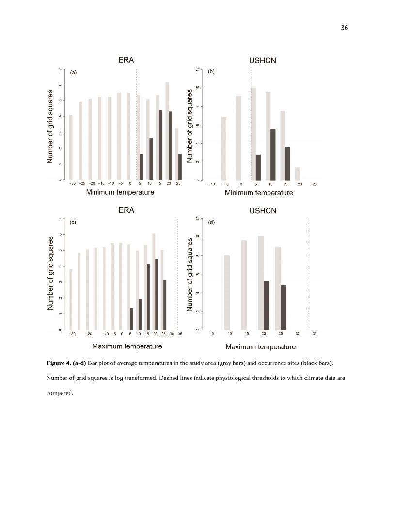
for minimum temperature of ~45 days. However, averaging climate data over the 22-year period,
temperatures at occurrence sites always fell within the optimal minimum temperature range
(Figure 4a).
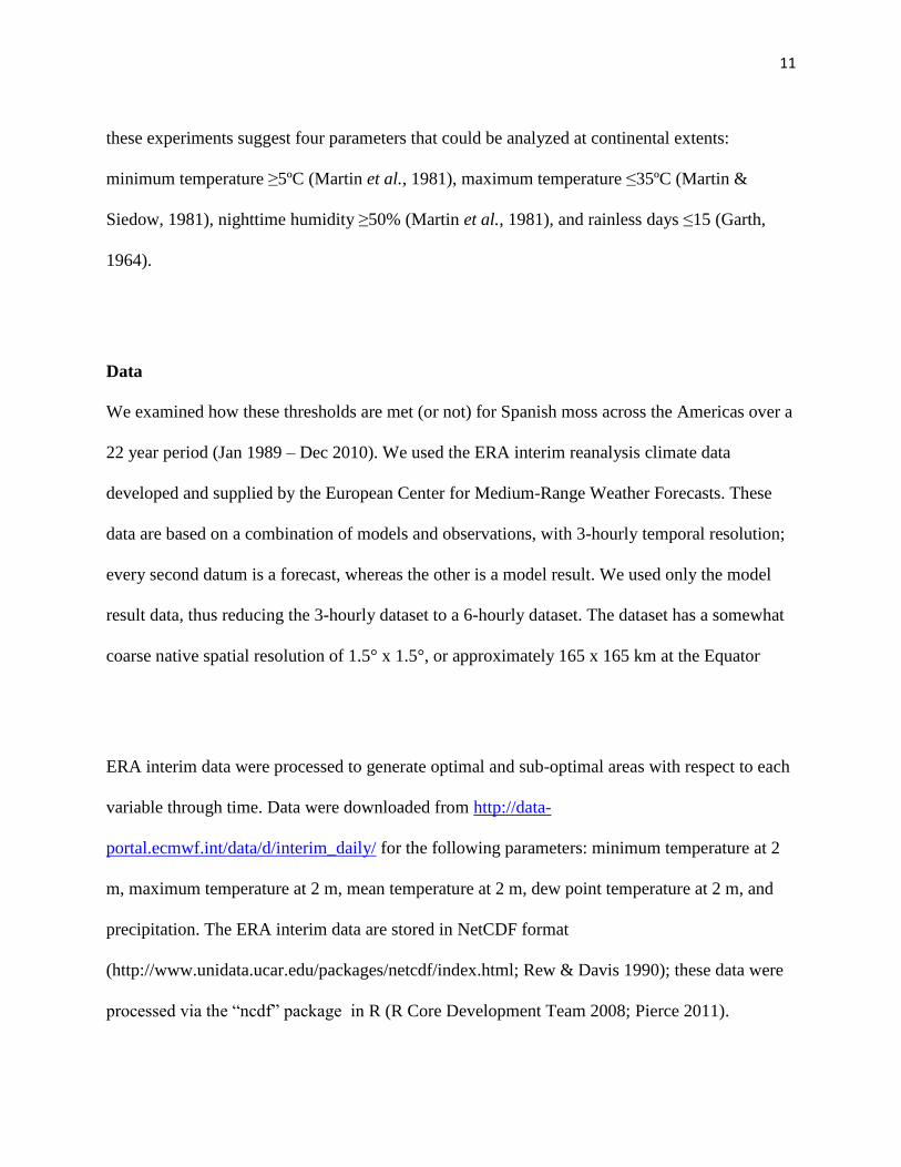
Maximum temperature depicts (Figure 5) an intriguing constraint: areas presenting optimal
maximum temperatures under single-day criteria were very small, with optimal maximum
temperatures available continuously only in western South America. High-latitude areas were not
affected by sub-optimal maximum temperatures, but tropical and sub-tropical areas were
severely constrained in this dimension. Indeed, increasing the number of days outside of the

17
optimal range up to 135 days still did not include all occurrences (see, e.g., occurrences in
Yucatan Peninsula and northern Brazil). The USHCN data similarly indicated that suitability for
maximum temperature must “alleviate” sub-optimal conditions for longer periods (i.e., >30 days)
to include most of the known occurrences of the species. However, 22-year average maximum
temperatures almost always were below 35°C (Figure 4c, 4d, 6d).
For precipitation, again, strict temporal limits (15 days) had to be relaxed, such that occurrences
are seen where rain occurs only at least every 30 days (Figure 2). Although the ERA data showed
the western edge of the distribution in the United States and Mexico as unsuitable even when the
temporal criterion was relaxed to 30 days, the finer-resolution USHCN data suggested that a
criterion of ~30 days suffices to include all occurrences. A period of ~20 days was required to
include the site where physiological measurements were taken.
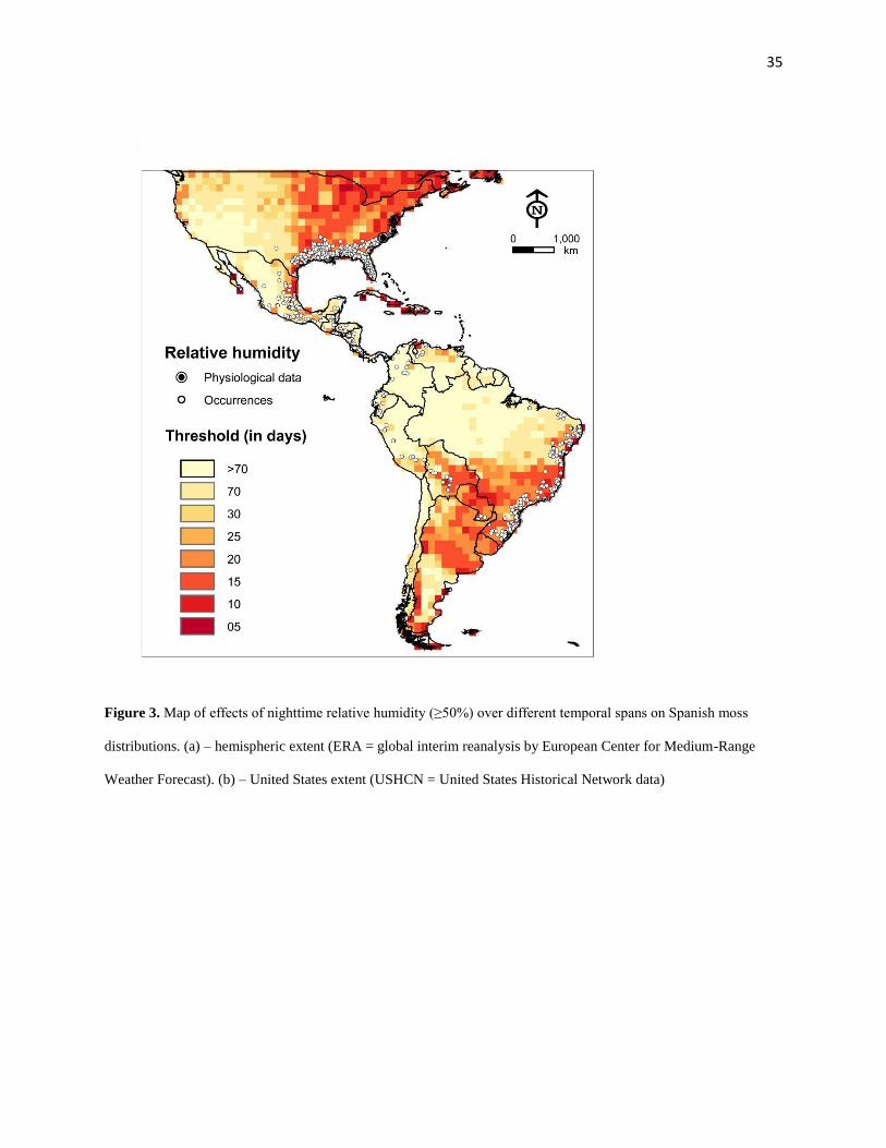
For relative humidity (Figure 3), the initial 5-day temporal criterion identified few grid squares
as suitable. The location where the physiological measurements were taken was within suitable
conditions at 15 days. However, to cover almost all of the known occurrences, ~70 days were
needed; even with a 70-day of temporal span, a few occurrences in Colombia, Peru, and Ecuador
were not covered under suitable areas. This result suggests that the ERA data are at such a coarse
resolution that the plants may encounter appropriate humidity microclimates.

18
To assess the result statistically, cumulative binomial probability tests assessing coincidence
between single-variable climate suitability maps and known occurrences of the species were
calculated in geographic space (Table 1). These probability values were significant for minimum
temperature at all temporal scales in the ERA data, but only over broader temporal scales for the
USHCN data. Probability values for rainless days were significant over all temporal scales for
both climate datasets. For maximum temperature, probability values were significant only at
single-day time scales in ERA, but also for longer scales in USHCN. Relative humidity showed
significance only for temporal scales of 1 and 5 days.
Our results also indicate that when temperatures are averaged, over long periods, populations
appear to experience optimal physiological thresholds, and the resultant picture appears much
more acceptable than when optimal conditions are assessed without averaging. Bar plots of
averaged data suggest that occurrence sites always experienced minimum temperature above 5ºC
and maximum temperatures below 35ºC (Figure 4) even when the raw data make clear that such
is frequently not the case.
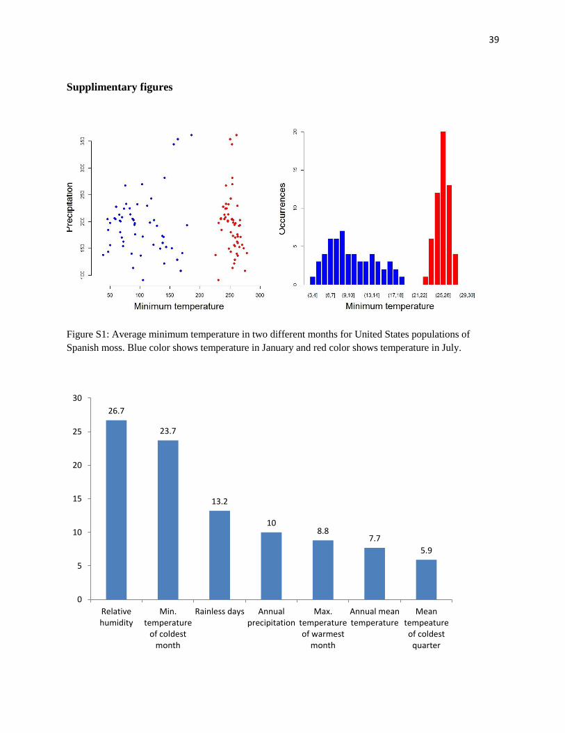
Among seven variables which are used in niche model calibration, relative humidity was
weighted most heavily in model calibration (See Figure S2 in supporting information). Viewing
our niche models as responses to environments, we see that more than 95% of Spanish moss
populations are always within optimal thresholds of temperature and relative humidity (Figure
6a-d, Figure S3). However, in the case of rainless days, many populations are not within optimal

19
thresholds. This figure effectively shows the effect of averaged climate data used in niche
models. Figure 4 (f) shows the potential distribution of Spanish moss populations throughout
Americas, based on niche model results.
Discussion
In our simple univariate testing scheme, climate data were processed in various environmental
dimensions to investigate temporal limits on Spanish moss occurrences. Physiological data are
measured on very fine scales of time and space (e.g., 10-3
-10-2
m), whereas climatic data are by
nature averaged broadly (~105 m) and can be difficult to develop at such fine scales for
hemispheric extents, owing to limited data availability and computational power (Potter et al.,
2013). Applying the physiological data across a hemisphere (as in this study) requires scaling at
two levels: scaling physiological thresholds from individuals to populations to global
distributions, and scaling from microclimates to macroclimates. Effects of physiological limits
on individuals could include reproductive failure, loss of mobility or shortened life spans.
Ribeiro et al. (2012) showed that effects of critical thermal limits on the recovery process in leaf-
cutting ants (Atta sexdens rubropilosa) depended on the time over which critical temperatures
were experienced, and how long and/or often those temperatures were experienced by the ants.
At the scale of populations, one can see that extreme conditions outside physiological limits may
affect population sizes, even causing local extirpation. At the species level, different
environments manifested across geographic distribution of species may create distinct selective
environments, under some circumstances leading to local physiological adaptation (Brady et al.,

20
2005). Hence scaling individual physiological tolerances to species entire distributional areas via
simple assumptions is likely to introduce error (Addo-Bediako et al., 2000).
Scaling from microclimate to macroclimate requires another set of assumptions, because
processes affecting microclimates are different from those affecting macroclimates. For example,
turbulence flux plays a role at fine scales that can be ignored at broader scales. Also, in
development of equations for scaling, parameters at fine scales may be well defined and
parameter relationships linear, but at broad scales relationships may be non-linear, owing to
influx of heat, moisture, and momentum over heterogeneous areas. Interactions between land and
atmosphere vary according to the scale of analysis, such that choosing the “right” scale is
impossible. If data are gathered from different localities, finding a proper method for data
aggregation is also a challenge (Brunsell & Gillies, 2003). Further, processes at different scales
receive feedback from each other, which influences processes and in turn this complicates the
system. Hence, while studies across diverse scales are essentials, integrating across these scales
poses significant challenges (Wu & Li, 2009).
As mentioned earlier, although microclimatic conditions affect individual organisms on quite
fine scales, many issues surround translation from microclimate and individual performance to
macroclimate and population persistence. In biophysical models, which are based on first
principles of growth and reproduction, physiological measurements are scaled to match available
climatic data (Kearney et al., 2008; Kearney & Porter, 2009). These approaches thus assume to

21
some degree that local landscapes are homogeneous. In reality, however, local landscapes are
highly heterogeneous, demanding approximations of parameters or broad assumptions regarding
parameter values (Lhomme, 1992), such that spatial resolution subsumes a major set of
assumptions of first-principles approaches to these issues. For Spanish moss, being an epiphyte
in tree canopies, heterogeneity of the landscape is particularly difficult to parameterize. The
effect of scaling is seen by contrasting our coarse (~165 km) ERA results with our fine-
resolution (10 km) USHCN results (Figures 1-3,5): imagine if climate data were available at
still-finer resolutions, such that we could capture these phenomena at biologically relevant
resolutions. Generating fine resolution climate data is a challenge, requiring active collaboration
among disciplines (Potter et al., 2013).
In correlative niche model applications, environmental data are frequently averaged by month or
year, and our results with such data indicated that modeled niches always tended to fall within
measured physiological limits (Figure 6). That is, species did not encounter their physiological
limits in correlative models owing to massive averaging of extremes in the climate data. On the
other hand, with fine-temporal-resolution data, most populations encounter suboptimal
conditions in at least one dimension. What is more, with these finer data, one can view the
species’ response against a broader range of conditions; in the averaged data, however, many of
the extremes are never manifested (see Figure 6, Figure S3), such that the existing fundamental
niche (i.e., the set of conditions manifested on geography) is notably smaller than the true
fundamental niche (i.e., that determined by the species’ physiology). Also, in many mechanistic
models, climate data are used as monthly averages, thus ignoring temporal scale and allowing

22
considerable information loss regarding temporal sequences, and thereby not taking fullest
advantage of the mechanistic approach (Buckley et al., 2010). The need for high temporal
resolution in environmental data used in mechanistic models has been acknowledged previously
(Kearney et al., 2012).
Hence, in this analysis, we are making use of high temporal-resolution climate data, and we are
not scaling physiological measurements in terms of particular environmental values, as any such
values would be guesses at best. Rather, we scale them in temporal terms, to understand how
long populations can persist under sub-optimal average conditions, at least in absence of local
adaptation (Martin et al., 1985), and then overlay available occurrence data from GBIF and
speciesLink to understand whether most populations are within suitable limits or not. Available
occurrence data suffice to outline major features of the species’ distribution, even though not all
populations are represented.
Martin et al. (1986) evaluated a few individuals of Spanish moss from sunny and shady locations
in South Carolina with different irradiance levels. Their research showed that these plants
respond physiologically to various irradiance levels, suggesting that Spanish moss adjusts
physiologically to the microclimates it inhabits, posing still more difficulty in generalizing
physiological responses from a few populations to entire distributions. In this paper, we
emphasize that, even when climate data are scaled temporally, not all populations appear to exist
under optimal conditions. Our result suggests (1) that optimal thresholds may be different in
23
different places, (2) that tolerance limit may be quite broad, (3) that suitable microhabitats are
not captured in the climate data, or (4) that temporal intervals of optimal conditions may need to
be relaxed still further. Use of physiological parameters from a single population has caveats due
to local adaptation or natural selection. To reduce the effect of local adaptation it is advisable to
collect physiological data from populations from widely-scattered geographic locations that
present distinct environmental conditions.
For example, for minimum temperature (Figure 1b), populations in North Carolina are within the
area presenting suitable conditions, but some populations in the southern Peruvian Andes fall
outside the limit. The degree to which local adaptation is involved in this model “failure” cannot
be assessed without direct experimentation, and to develop a robust model, physiological data
from populations in the unsuitable category would be very informative. Buckley et al. (2008)
compared performance of biophysical and correlative approaches in anticipating range shifts
under climate change scenarios, and concluded that projected range shifts were more pronounced
in mechanistic models as compared to correlational models. However, to parameterize
mechanistic models, many assumptions were required, such that comparisons of these two
approaches are perhaps best considered as speculative. In applying measured physiological
thresholds from one or a few locations to broad distributional areas in this study, we see that
ecophysiological approaches have significant limitations as well. Because physiological
measurements are taken at one or a few sites only, any local adaptation will not be taken into
account in estimates of distributions, and projections of parameters may frequently fail to include
all populations.
24
Our results also suggest an interesting contrast: Spanish moss populations can persist outside of
optimal minimum temperature ranges for a few days, but can withstand sub-optimal thresholds
for maximum temperatures for longer periods. Clearly, sub-optimal conditions in the growing or
flowering season might have different implications than at other times. For example, the specific
importance of conditions during particular life stages of insect populations has long been
appreciated (Wellington, 1956). Clearly, if the species cannot reproduce in a place, it is not going
to occupy that region, so, non-optimal conditions in the growing season may constitute a more
specific constraint on the distribution of Spanish moss (See Figure S1 in Supporting
Information). When the occurrence data are plotted against the average climate data (Figure 6),
about 95% of the populations come within optimal physiological ranges. Our approach thus
stresses the importance of using temporally fine-scale climate data for analysis, particularly
when integrating physiology of species in the model.
The approach used here is not considering interaction of variables for a simple reason: as
physiological limits data are usually assessed for different variables independently, these
experiments assume other variables at constant value, although a few studies have attempted to
assess physiological responses to multiple variables (Johnson et al., 1997). The difficulty in
capturing multi-variable responses lies in time investment required for experiments. Also, many
times, particular combinations of variable values may not exist in the real world, yet interaction
of variables may play important roles in limiting distributions of species. Smith (2013) examined
the role of interactions of temperature and precipitation in constraining ranges of 67 mammalian

25
species; their results indicated that interactions between the two climate dimensions play
important roles in shaping the distributions of 85% of the species.
Ecophysiologists measure either optimal thresholds or tolerance limits for environmental
parameters (Martin & Siedow, 1981; Martin et al., 1981; Huey & Hertz, 1984; Angilletta et al.,
2010), which must be pondered if their results are to be used in these geographic views. Such
studies cover only a few variables, and each variable is generally assessed independently of
others, so using this information directly in biophysical models can be complex, because only a
subset of key parameters is measured. Several studies have begun using biophysical data for
estimating niches and distributions, yet physiological data are available from a relatively few
species only. For example, Kearney et al. (2008), explored potential distributions of an invasive
toad species in Australia based on biophysical parameters, but measurements were available only
for adults, and only for invasive populations: characterizing these additional measurements
would involve considerable time and resources. Hence, notwithstanding that biophysical
measurements may be (in theory, at least) excellent ways to characterize fundamental niches,
their application in practice is not straightforward.
Although this approach can be used to understand the physiological constraints on the
populations, but cannot be used so readily to predict the distributions of species per se, the
approach used here provides valuable insights into, and leads to new questions about, the biology
and ecophysiology of the species under investigation. For example, when populations of the
26
species occur well outside the physiologically optimal environmental conditions (e.g., Spanish
moss populations in Brazil, Baja California, and central Mexico; Figures 4 and 5), are
individuals in these populations under severe stress and growing poorly, or do these individuals
possess unique ecophysiological features that prove adaptive in these putatively sub-optimal
environments? Answers to such questions may well provide novel views of the physiology and
natural history that may otherwise be impossible to obtain.
Acknowledgements
We are thankful to three anonymous reviewers for helpful comments. We are grateful to Jorge
Soberón for insightful discussions. ATP and NB was supported by a grant from Microsoft
Research.
References
Addo-Bediako, A., Chown, S.L. & Gaston, K.J. (2000) Thermal tolerance, climatic variability
and latitude. Proceeding of the Royal Society, 267, 739–745.
Angilletta, M.J., Huey, R.B. & Frazier, M.R. (2010) Thermodynamic effects on organismal
performance: is hotter better? Physiological and Biochemical Zoology, 83, 197–206.
Billings, F.H. (1904) A study of Tillandsia usneoides. Botanical Gazette, 38, 99–121.
Bivand, R.S., Pebesma, E.J. & Gómez-Rubio, V. (2008) Applied spatial data analysis with R,
Springer, New York.

27
Brady, K.U., Kruckeberg, A.R. & Bradshaw Jr., H.D. (2005) Evolutionary ecology of plant
adaptation to serpentine soils. Annual Review of Ecology, Evolution, and Systematics, 36,
243–266.
Brunsell, N.A. & Gillies, R.R. (2003) Scale issues in land–atmosphere interactions: implications
for remote sensing of the surface energy balance. Agricultural and Forest Meteorology,
117, 203–221.
Buckley, L.B. (2008) Linking traits to energetics and population dynamics to predict lizard
ranges in changing environments. American Naturalist, 171, E1–E19.
Buckley, L.B., Urban, M.C., Angilletta, M.J., Crozier, L.G., Rissler, L.J. & Sears, M.W. (2010)
Can mechanism inform species’ distribution models? Ecology Letters, 13, 1041–1054.
Callaway, R.M., Reinhart, K.O., Moore, G.W., Moore, D.J. & Pennings, S.C. (2002) Epiphyte
host preferences and host traits: mechanisms for species-specific interactions. Oecologia,
132, 221–230.
Chapman, A.D. (2005) Principles and methods of data cleaning—primary species and species-
occurrence data, Global Biodiversity Information Facility, Copenhagen.
Diggle, P.J., Ribeiro Jr, P.J. & Christensen, O.F. (2003) An introduction to model-based
geostatistics. Spatial statistics and computational methods (ed. by J. Møller), p. 224.
Springer-Verlag, New York.
Diggle, P.J. & Ribeiro Jr., P.J. (2007) Model-based geostatistics, Springer-Verlag, New York.
Garth, R.E. (1964) The ecology of Spanish moss (Tillandsia usneoides): its growth and
distribution. Ecology, 45, 470–481.
Gentry, A.H. & Dodson, C.H. (1987) Diversity and biogeography of Neotropical vascular
epiphytes. Annals of the Missouri Botanical Garden, 74, 205–233.

28
Hijmans, R.J. & van Etten, J. (2012) raster: Geographic analysis and modeling with raster data.
http://CRAN.R-project.org/package=raster
Hijmans, R.J., Phillips, S., Leathwik, J. & Elith, J. (2012) dismo: species distribution modeling.
http://CRAN.R-project.org/package=dismo
Huey, R.B. & Hertz, P.E. (1984) Is a jack-of-all-temperatures a master of none? Evolution, 38,
441–444.
Hyndman, R.J. & Koehler, A.B. (2006) Another look at measures of forecast accuracy.
International Journal of Forecasting, 22, 679–688.
Johnson, J.D., Tognetti, R., Michelozzi, M., Pinzauti, S., Minotta, G. & Borghetti, M. (1997)
Ecophysiological responses of Fagus sylvatica seedlings to changing light conditions. II.
The interaction of light environment and soil fertility on seedling physiology. Physiologia
Plantarum, 101, 124–134.
Kearney, M.R., Phillips, B.L., Tracy, C.R., Christian, K.A., Betts, G. & Porter, W.P. (2008)
Modelling species distributions without using species distributions: the cane toad in
Australia under current and future climates. Ecography, 31, 423–434.
Kearney, M.R. & Porter, W.P. (2004) Mapping the fundamental niche: physiology, climate, and
the distribution of a nocturnal lizard. Ecology, 85, 3119–3131.
Kearney, M.R., Matzelle, A. & Helmuth, B. (2012) Biomechanics meets the ecological niche:
the importance of temporal data resolution. The Journal of Experimental Biology, 215, 922–
933.
Kearney, M.R. & Porter, W.P. (2009) Mechanistic niche modelling: combining physiological
and spatial data to predict species’ ranges. Ecology Letters, 12, 334–350.

29
Kluge, M., Lange, O.L., Eichman, M.. & Schmid, R. (1973) Diurnaler säurerhythmus bei
Tillandisa usneoides: Untersuchungen über Weg des Kohlenstoffs sowie die Abhängigkeit
des CO2 - Gaswechsels von Lichtintensitat, temperature und Wessergehalt der Pflanze.
Planta, 112, 357–372.
Kreft, H., Köster, N., Küper, W., Nieder, J. & Barthlott, W. (2004) Diversity and biogeography
of vascular epiphytes in western Amazonia, Yasunı, Ecuador. Journal of Biogeography, 31,
1463–1476.
Lhomme, J. (1992) Energy balance of heterogeneous terrain: averaging the controlling
parameters. Agricultural and Forest Meteorology, 61, 11–21.
Martin, C.E., Christensen, N.L. & Strain, B.R. (1981) Seasonal patterns of growth, tissue acid
fluctuations, and 14
CO2 uptake in the Crassulacean Acid Metabolism epiphyte Tillandsia
usneoides L. (Spanish moss). Oecologia, 49, 322–328.
Martin, C.E., Eades, C.A. & Pitner, R.A. (1986) Effects of irradiance on Crassulacean Acid
Metabolism in the epiphyte Tillandsia usneoides L. (Bromeliaceae). Plant Physiology, 80,
23–26.
Martin, C.E., McLeod, K.W., Eades, C.A. & Pitzer, A.F. (1985) Morphological and
physiological responses to irradiance in the CAM epiphyte Tillandsia usneoides L.
(Bromeliaceae). Botanical Gazette, 146, 489–494.
Martin, C.E. & Schmitt, A.K. (1989) Unusual water relations in the CAM atmospheric epiphyte
Tillandsia usneoides L. (Bromeliaceae). Botanical Gazette, 150, 1–8.
Martin, C.E. & Siedow, J.N. (1981) Crassulacean Acid Metabolism in the epiphyte Tillandsia
usneoides L. (Spanish moss): Responses of CO2 exchange to controlled environmental
conditions. Plant Physiology, 68, 335–339.
30
Peterson, A.T., Soberón, J., Pearson, R.G., Anderson, R.P., Martinez-Meyer, E., Nakamura, M.
& Araújo, M.B. (2011) Ecological niches and geographic distributions, Princeton
University Press, Princeton, New Jersey.
Phillips, S.J., Anderson, R.P. & Schapire, R.E. (2006) Maximum entropy modeling of species
geographic distributions. Ecological Modelling, 190, 231–259.
Pierce, D. (2011) ncdf: Interface to Unidata netCDF data files. http://CRAN.R-
project.org/package=ncdf
Porter, W.P. & Mitchell, J.W. (2006) Method and system for calculating the spatial-temporal
effects of climate and other environmental conditions on animals. US patent no 7,155,377
Porter W.P., Mitchell, J.W., Beckman, W.A. & Dewitt, C.B. (1973) Behavioral implications of
mechanistic ecology. Thermal and behavioral modeling of desert ectotherms and their
microenvironment. Oecologia, 13, 1–54.
Porter, W.P., Sabo, J.L., Tracy, C.R., Reichman, O.J. & Ramankutty, N. (2002) Physiology on a
landscape scale: plant-animal interactions. Integrative and Comparative Biology, 42, 431–
453.
Potter, K.A., Woods, H.A. & Pincebourde, S. (2013) Microclimatic challenges in global change
biology. Global Change Biology, 2932–2939.
Rew, R. & Davis, G. (1990) NetCDF: An interface for scientific data access. IEEE Computer
Graphics and Applications, 10, 76–82.
Ribeiro, P.L., Camacho, A. & Navas, C.A. (2012) Considerations for assessing maximum critical
temperatures in small ectothermic animals: insights from leaf-cutting ants. PLoS ONE, 7,
e32083.
31
Ribeiro, R.J. & Diggle, P.J. (2001) geoR: A package for geostatistical analysis. R News, 1, 15–
18.
Saupe, E.E., Barve, V., Myers, C.E., Soberón, J., Barve, N., Hensz, C.M., Peterson, A.T.,
Owens, H.L. & Lira-Noriega, A. (2012) Variation in niche and distribution model
performance: the need for a priori assessment of key causal factors. Ecological Modelling,
237-238, 11–22.
Smith, A.B. (2013) The relative influence of temperature, moisture and their interaction on range
limits of mammals over the past century. Global Ecology and Biogeography, 22, 334–343.
Soberón, J. (2007) Grinnellian and Eltonian niches and geographic distributions of species.
Ecology Letters, 10, 1115–1123.
Soberón, J. & Peterson, A.T. (2005) Interpretation of models of fundamental ecological niches
and species distributional areas. Biodiversity Informatics, 2, 1–10.
Stull, R.B. (1988) An introduction to boundary layer meterology, Springer-Verlag, New York.
The R Core Development Team (2012) R: A language and environment for statistical computing.
Wellington, W.G. (1956) The synoptic approach to studies of insects and climate. Annual Review
of Entomology, 2, 143–162.
Wu, H. & Li, Z.-L. (2009) Scale issues in remote sensing: a review on analysis, processing and
modeling. Sensors, 9, 1768–1793.
Young, O.P. & Lockley, T.C. (1989) Spiders of Spanish moss in the delta of Mississippi. Journal
of Arachnology, 17, 143–148.

32
Table 1: p-values of cumulative binomial probability tests used to assess coincidence between
occurrences and suitable areas as per minimum temperature, maximum temperature, rainless
days and relative humidity thresholds. – indicates no data availability, ERA = global interim
reanalysis by European Center for Medium-Range Weather Forecast, USHCN = United States
Historical Climate Network.
Days
Minimum
temperature (5°C)
Maximum
temperature (35°C)
Rainless days Relative
humidity (50%)
ERA USHCN ERA USHCN ERA USHCN ERA
1 0.001 0.001 0.001 0.001 - - 0.001
5 0.001 0.15 1.00 1.00 - - 0.067
10 0.001 0.23 1.00 1.00 - - 1.00
15 0.001 0.001 1.00 0.99 0.001 0.001 1.00
20 0.001 0.001 1.00 0.69 0.001 0.001 1.00
25 0.001 0.001 1.00 0.002 0.001 0.001 1.00
30 0.001 0.001 1.00 0.011 0.001 0.001 1.00
45 - 0.001 - - - - -
70 - - - - - - 1.00
135 - - 1.00 - - - -

33
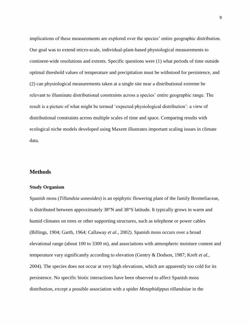
Figure 1. Map of effects of minimum temperature thresholds (≥5°C) over different temporal spans on
Spanish moss distributions. (a) – hemispheric extent (ERA = global interim reanalysis by European
Center for Medium-Range Weather Forecast). (b) – United States extent (USHCN = United State
Historical Climate Network data)

34
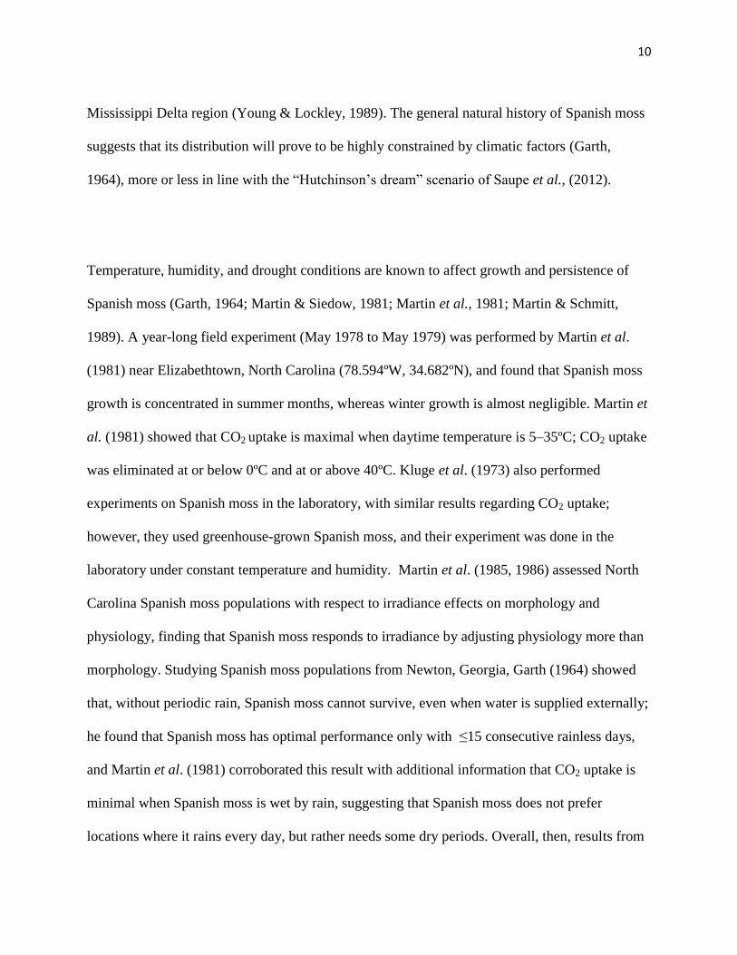
Figure 2. Map of effects of rainless days (≤15 days) over different temporal spans on Spanish moss distributions. (a)
– hemispheric extent (ERA = global interim reanalysis by European Center for Medium-Range Weather Forecast).
(b) – United States extent (USHCN = United States Historical Climate Network data).
35
Figure 3. Map of effects of nighttime relative humidity (≥50%) over different temporal spans on Spanish moss
distributions. (a) – hemispheric extent (ERA = global interim reanalysis by European Center for Medium-Range
Weather Forecast). (b) – United States extent (USHCN = United States Historical Network data)
36
Figure 4. (a-d) Bar plot of average temperatures in the study area (gray bars) and occurrence sites (black bars).
Number of grid squares is log transformed. Dashed lines indicate physiological thresholds to which climate data are
compared.

37
Figure 5. Map of effects of maximum temperature thresholds (≤35°C) over different temporal spans on Spanish
moss distributions. (a) – hemispheric extent (ERA = global interim reanalysis by European Center for Medium-
Range Weather Forecast). (b) – United States extent (USHCN = United States Historical Climate Network data)

38
Figure 6. (a-e) Scatter plot of suitability and variables used in the correlative Maxent model. Gray dots show
environments represented across the study area. Black dots show occurrences. The dotted lines show the location of
95% of occurrences. The gray box outlines optimal physiological limits. Panel (f) shows the potential suitability of
Spanish moss using Maxent.
39
Supplimentary figures
Figure S1: Average minimum temperature in two different months for United States populations of
Spanish moss. Blue color shows temperature in January and red color shows temperature in July.
26.7
23.7
13.2
10 8.8
7.7
5.9
0
5
10
15
20
25
30
Relativehumidity
Min.temperature
of coldestmonth
Rainless days Annualprecipitation
Max.temperatureof warmest
month
Annual meantemperature
Meantempeatureof coldest
quarter
40
Figure S2 : Bar plot of variable contributions in the Maxent model.
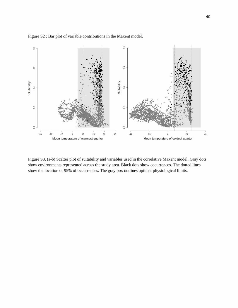
Figure S3. (a-b) Scatter plot of suitability and variables used in the correlative Maxent model. Gray dots
show environments represented across the study area. Black dots show occurrences. The dotted lines
show the location of 95% of occurrences. The gray box outlines optimal physiological limits.
41
Chapter 2
Climatic Niches and Flowering and Fruiting
Phenology of Spanish moss (Tillandsia
usneoides)

42
Abstract
Species have geographic distributions constrained by combinations of abiotic factors, biotic
factors, and dispersal-related factors. Abiotic requirements vary across the life stages for a
species; for plant species, a particularly important life stage is when the plant flowers and
develops seeds. A previous year-long experiment showed that ambient temperature of 5-35°C,
relative humidity of >50% and <15 consecutive rainless days are crucial abiotic conditions for
Spanish moss (Tillandsia usneoides). Here, we explore whether these optimal physiological
intervals relate to the timing of the flowering and fruiting period of Spanish moss across its
range. As Spanish moss has a broad geographic range, we examined herbarium specimens to
detect and characterize flowering/fruiting periods for the species across the Americas; we used
high-temporal-resolution climatic data to assess the availability of optimal conditions for Spanish
moss populations during each population’s flowering period. We explored how long populations
experience sub-optimal conditions, and found that most populations experience sub-optimal
conditions in at least one environmental dimension. Flowering and fruiting periods of Spanish
moss populations are either being optimized for one or a few parameters, or may be adjusted
such that all parameters are sub-optimal. Spanish moss populations appear to be constrained
most closely by minimum temperature during this period.

43
Introduction
Restricted geographic distributions of species are often a consequence of some set of
constraints in terms of abiotic requirements, needs in terms of biotic interactions, and limitations
to dispersal ability (Soberón, 2007). All species have a life cycle (be it simple or complex), and
each stage in that cycle may have different requirements in terms of climate, soils, topography,
other abiotic factors, and biotic requirements like food, competitors, or mutualisms. Grubb
(1977) defined 4 components of ecological niches of plants: the habitat niche, life-form niche,
phenological niche, and regeneration niche; much research has examined how regeneration
niches may differ in different community assembly processes, and how these various niches act
in different life stages (Fowler, 1988; Lavorel & Chesson, 1995; Miller-Rushing & Primack,
2008; Tilman, 2014). Although several studies have used the regeneration niche concept to
explore competition and understand rarity of species at local scales (Engelhardt & Anderson,
2011; Ranieri et al., 2012), few studies have used the regeneration niche idea to understand
species’ distributions in terms of their abiotic requirements at geographic scales (Pederson et al.,
2004; Sweeney et al., 2006; Wellenreuther & Arson, 2012).
Phenological stages in plant life cycles comprise critical life stages, in which plants
flower, produce seeds, grow, or remain dormant (Bond & Midgley, 2001; Silvertown, 2004).
Plants have presumably evolved to flower in seasons and at intervals that ensure maximal
reproductive success (Amasino, 2010). Considerable research has shown that plants sense and
respond in complex ways to environmental cues (Garner, 1933; Lang, 1952; Bernier et al., 1993;
Dennis et al., 1996). However, these factors have been investigated chiefly at local scales; at
biogeographic scales, the question of whether phenology is optimized or not with respect to
44
physiological responses to abiotic factors like temperature and precipitation remains little
investigated (Engelhardt & Anderson, 2011; Ranieri et al., 2012).
Here, we examine the timing of flowering and fruiting by Spanish moss (Tillandsia
usneoides) populations across the species’ broad geographic range in relation to availability of
optimal physiological conditions (Barve et al., 2014). Physiological measurements have been
made in yearlong field experiments (Martin & Siedow, 1981; Martin et al., 1981) to estimate
ideal intervals of climate-related parameters. We used herbarium specimen records of flowering
and fruiting Spanish moss to identify population-specific flowering and fruiting periods, and
tested detailed environmental data for associations with minimum temperature, maximum
temperature, relative humidity, and rainless days requirements on a univariate basis, building on
our earlier analyses of physiological limits in relation to climate across the range of this species
(Barve et al., 2014). We use these analyses to test whether (1) all four parameters are at optimal
physiological values as measured in previous studies during flowering periods, and (2) which
physiological parameter(s) is (are) optimized during the flowering periods, if not all are
optimized.
Methods
Study Organism
Spanish moss (Tillandsia usneoides) is an epiphytic flowering plant of the family
Bromeliaceae, distributed approximately between 38°N and 38°S latitude. It typically grows in
warm and humid climates on trees or other supporting structures, such as power cables (Billings,

45
1904; Garth, 1964; Callaway et al., 2002). Spanish moss occurs over a broad elevational range
(0–3300 m), and associations with atmospheric moisture content and temperature vary
significantly according with elevation (Gentry & Dodson, 1987; Kreft et al., 2004). The species
does not occur at high elevations, which are apparently too cold for its persistence; indeed, its
general natural history suggests that its distribution will prove to be highly constrained by
climatic factors (Garth, 1964), more or less in line with the “Hutchinson’s dream” scenario of
Saupe et al. (2012).
Temperature, humidity, and drought are known to affect growth and persistence of
Spanish moss (Garth, 1964; Martin & Siedow, 1981; Martin et al., 1981; Martin & Schmitt,
1989). A year-long field experiment (May 1978 to May 1979) was performed by Martin et al.
(1981) near Elizabethtown, North Carolina (78.594°W, 34.682°N); it found that Spanish moss
growth is concentrated in summer months, with winter growth almost negligible. Martin et al.
(1981) showed that CO2 uptake was maximal when daytime temperature is 5–35ºC; CO2 uptake
was eliminated at or below 0ºC and at or above 40ºC. Kluge et al. (1973) also experimented on
Spanish moss, with similar results regarding CO2 uptake; however, they used greenhouse-grown
Spanish moss, and their experiment was carried out in the laboratory under constant temperature
and humidity. Martin et al. (1985, 1986) assessed North Carolina Spanish moss populations with
respect to irradiance effects on morphology and physiology, finding that Spanish moss responds
to irradiance by adjusting physiology more than morphology. Garth (1964) showed that Spanish
moss cannot survive in Georgia without periodic rainfall, even when water is supplied externally;
he found that Spanish moss achieves optimal performance in terms of growth only with ≤15
consecutive rainless days. Martin et al. (1981) corroborated this latter result, with the additional
information that CO2 uptake is minimal when Spanish moss is wet by rain, suggesting that

46
Spanish moss requires some dry periods for persistence. Overall, then, these experiments
identified four parameters that can be analyzed at continental extents: minimum temperature
≥5ºC (Martin et al., 1981), maximum temperature ≤35ºC (Martin & Siedow, 1981), nighttime
humidity ≥50% (Martin et al., 1981), and ≤15 rainless days (Garth, 1964).
Input Data
We collected information on flowering and fruiting periods of Spanish moss populations
by examining herbarium specimens. We photographed 430 specimens in the collections of the
Missouri Botanical Garden and 504 specimens from the New York Botanical Garden collections
using a 16 megapixel Nikon P510 camera. We took 3–4 photographs per specimen to capture
various details: one of the label to permit capture of associated data, one of the whole specimen,
and 2–3 zoomed photographs of flowers or fruits. In addition, we reviewed published floras for
flowering dates, although most floras either did not offer sufficient detail about flowering period,
or do not provide precise locality information. Finally, we downloaded images from various
herbaria listed on the Index Herbariorum site
(http://sciweb.nybg.org/science2/IndexHerbariorum.asp) and others
(http://herbarium.bio.fsu.edu, http://apps.kew.org/herbcat/navigator.do). Flowering and fruiting
periods were assumed to be unimodal, so we filled temporal gaps for analyses of optimal
physiological conditions. The temporal resolution of flowering and fruiting times was kept at
months, so that imprecise date information (e.g., “April 1914”) could be incorporated, and
quantity of relevant data maximized.

47
Information from specimen labels was digitized and stored in a Microsoft Access
database. Some labels had geolocations in terms of latitude-longitude coordinates, whereas
others had only textual locality information at various administrative levels. In the latter case,
geolocations were attached to each record via queries in Google Earth. Overall, we were able to
obtain information for 361 sites where both flowering date and geolocations information was
available, which we used to profile flowering/fruiting periods at sites across the range of the
species.
We examined how physiological thresholds are met (or not) for Spanish moss across the
Americas within empirically documented flowering intervals over a 22-year period (January
1989 – December 2010) following Barve et al. (2014). We used the ERA interim reanalysis
climate data developed and supplied by the European Center for Medium-Range Weather
Forecasts, which are based on a combination of models and observations, with 3-hourly temporal
resolution: every second datum is a forecast, whereas the other is a model result. We used only
the model result data, thus coarsening the data from 3-hourly to 6-hourly resolution, but retaining
an impressively fine temporal resolution. The dataset has a somewhat coarse native spatial
resolution of 1.5° x 1.5° or approximately 165 x 165 km grid square resolution at the Equator.
ERA Data were downloaded from http://apps.ecmwf.int/datasets/data/interim_full_daily/
for the following parameters: minimum temperature at 2 m, maximum temperature at 2 m, mean
temperature at 2 m, dew point temperature at 2 m, and precipitation. The data are stored in
NetCDF format (http://www.unidata.ucar.edu/packages/netcdf/index.html; Rew & Davis 1990);
these data were manipulated and processed via the “ncdf” package in R (Pierce, 2011; R Core
Development Team, 2012). ERA interim data were processed to identify optimal and sub-
48
optimal areas and temporal duration of sub-optimal conditions with respect to each physiological
variable through time.
Overall, 136 1.5° grid squares held at least one Spanish moss record with flowering and
fruiting information. As numbers of flowering records were not numerous with respect to so
many grid squares, to improve data density, we coarsened the 1.5° grid to 3° grids only to
characterize flowering periods, but climate data were kept at the original 1.5° resolution. We
generated flowering and fruiting month ranges for each 3° grid square; we assumed single
flowering/fruiting months in grid squares in which only single specimens were available, which
may be a restrictive assumption in our analyses. We also generated non-flowering month datasets
for each grid square for comparison; for example, for a grid square with a flowering/fruiting
range of March-May, we generated the remaining 11 possible three-month sequences for
comparison. We identified the average flowering/fruiting month, flowering/fruiting season start,
and flowering/fruiting season end for each grid square. Average flowering/fruiting month was
calculated as a weighted average based on number of flowering or fruiting specimens in each
month.
Data Analysis
An R script was developed using the raster, ncdf, and sp packages (Bivand et al., 2008;
Pierce, 2011; Hijmans & van Etten, 2012) to calculate the percentage of time over the 22-year
span of the data set that Spanish moss populations experienced optimal conditions with respect to
the physiological thresholds described above. For minimum and maximum temperatures, the
script checks the value of each variable across four daily observations; a grid square was marked

49
as unsuitable for a day whenever two consecutive observations were outside the limit. For
precipitation, whenever all four daily observations were 0 (i.e., no precipitation), it was
considered as a day with no precipitation, and all consecutive sets of 15 days were checked;
when any 15-day period had no precipitation, the grid square was considered as not suitable. For
relative humidity, dew point temperature (Td) and mean air temperature at 2 m (Ta) were used,
and relative humidity was calculated as Rh = es(Td)/es(Ta), or the ratio of saturation vapor
pressure at dew point to that at air temperature, where es for any temperature T is given by es(T) =
6.112*e(17.502*T / (240.97 +T))
(Stull, 1988). We identified grid cells as unsuitable whenever two
consecutive observations fell below the humidity threshold. Likewise, we calculated the
percentage of time that the grid square spent outside its optimal physiological thresholds within
the flowering period for that grid square across the 22-year time span; for comparison, we also
generated these percentages for all possible non-flowering periods of similar duration.
We ranked each grid square based on the percentage of time spent outside optimal values
in flowering and fruiting periods and each other possible non-flowering period of similar
duration. We calculated the rank of each of the observed flowering periods with respect to all
other possible periods of the same duration as the number of time periods of non-flowering
months that are more suitable. We used Kolmogorov-Smirnov test to compare distributions of
the four variable ranks.
Based on ranks of each grid square for each of the variables, we compared the actual
flowering period with the optimum flowering and fruiting period with respect to those variables.
This distance was calculated as a Euclidian distance from an optimal rank of 1 for each of the
variables, such that small distances indicate optimal flowering and fruiting periods for a

50
population, whereas large distances suggest that the population flowers during suboptimal
periods. We averaged this distance across all 4 physiological parameters, and mapped these
deviations from optimum. We tested for effects of number of herbarium specimen records in
each grid square to these optimum distances.
Results
We were able to assemble 361 flowering or fruiting records for Spanish moss across the
species’ range. Although records concentrated in the US portion of the species’ range (159
records, or 44%), the remaining 202 (56%) records came from Latin America. Although
densities of Latin American points were low at finer spatial resolutions (i.e., most grid squares
had single or no flowering-period records), 3° spatial resolution was sufficient to create 83 grid
squares, within which we had 1–28 flowering/fruiting records.
Average flowering and fruiting month of Spanish moss populations across the species’
range is shown in Figure 1. The flowering and fruiting period in eastern Brazil was November to
April, while the flowering and fruiting period in western South America was June to September,
with a few exceptions extending to October-November. The flowering period in the US and
Mexico was May to September, with a few exceptions in November-December. Because our
identification of flowering and fruiting month(s) was in some sense dependent on numbers of
specimens available, we suspect that insufficient data density may be driving the exceptions.
Flowering periods invariably fell in time periods in which least one physiological
parameter was optimal in a grid square. The “optimal” parameter was generally minimum
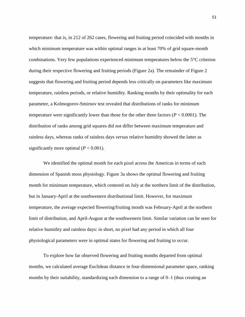
51
temperature: that is, in 212 of 262 cases, flowering and fruiting period coincided with months in
which minimum temperature was within optimal ranges in at least 70% of grid square-month
combinations. Very few populations experienced minimum temperatures below the 5°C criterion
during their respective flowering and fruiting periods (Figure 2a). The remainder of Figure 2
suggests that flowering and fruiting period depends less critically on parameters like maximum
temperature, rainless periods, or relative humidity. Ranking months by their optimality for each
parameter, a Kolmogorov-Smirnov test revealed that distributions of ranks for minimum
temperature were significantly lower than those for the other three factors (P < 0.0001). The
distribution of ranks among grid squares did not differ between maximum temperature and
rainless days, whereas ranks of rainless days versus relative humidity showed the latter as
significantly more optimal (P < 0.001).
We identified the optimal month for each pixel across the Americas in terms of each
dimension of Spanish moss physiology. Figure 3a shows the optimal flowering and fruiting
month for minimum temperature, which centered on July at the northern limit of the distribution,
but in January-April at the southwestern distributional limit. However, for maximum
temperature, the average expected flowering/fruiting month was February-April at the northern
limit of distribution, and April-August at the southwestern limit. Similar variation can be seen for
relative humidity and rainless days: in short, no pixel had any period in which all four
physiological parameters were in optimal states for flowering and fruiting to occur.
To explore how far observed flowering and fruiting months departed from optimal
months, we calculated average Euclidean distance in four-dimensional parameter space, ranking
months by their suitability, standardizing each dimension to a range of 0–1 (thus creating an

52
index of distance that has rather unclear units but that is useful for visualization), and counting
ranks as greater distance from optimal conditions (Figure 4). Most populations (46%) showed
flowering and fruiting periods with Euclidean distances of <0.5. Only a few pixels were under
extremely bad conditions and these higher-distance populations were arrayed at the extremes of
the distribution (Figure 4). We tested whether number of available flowering/fruiting specimens
affected these latter results (see scatterplot inset in Figure 4), but found no effect of sample size
on distance to optimal month.
Discussion
In overview, we found that Spanish moss populations appear to ‘tune’ their phenological
niches such that they experience optimum minimum temperatures for most of their respective
flowering and fruiting periods. Among populations analyzed, flowering and fruiting periods of
about 76% of Spanish moss populations experienced optimal minimum temperatures when
compared with other time periods through the year. Conversely, Spanish moss populations
appear to flower and fruit without much consideration of optimality of maximum temperature or
relative humidity optimality, though rainless days do have some importance.
Numerous recent studies have documented shifts in flowering and fruiting season as a
consequence of climate change (Telemeco et al., 2013; Molau et al., 2005; Miller-Rushing &
Primack, 2008). Veriankaite et al. (2010) explored optimum temperatures for flowering and
fruiting by comparing air temperatures in climate models with long-term flowering data.
However, for this study, we took advantage of known optimum physiological parameters (Martin

53
et al., 1981; Martin & Siedow, 1981; Martin & Schmitt, 1989), so we could explore the degree to
which Spanish moss flowering and fruiting periods coincide with months presenting optimal
physiological conditions for growth.
Phenological differences are well documented as functions of elevation and latitude
(Ruml et al., 2011; CaraDonna et al., 2014). However, we generated our phenological
information from herbarium specimens: few had elevation information, so effects of elevation on
flowering phenology cannot be examined particularly in light of the coarse spatial resolution of
our weather data. Clearly, as the climate data are coarsened and averaged over broader extents,
such details average out in the climate and become invisible to our analyses, as was noted in our
previous analyses (Barve et al., 2014). Our analyses may also be compromised by our rather
coarse characterization of flowering and fruiting periods (i.e., to month), and by our filling of
temporal gaps in flowering periods under the assumption of a single, continuous flowering and
fruiting period for each population.
Hadley et al., (1984) observed that elevated maximum temperatures can delay flowering,
in effect slowing down the reproduction in soybeans (Glycine max). However, for Spanish moss,
we observed that flowering phenology does not generally depend much on maximum
temperature. Rather, minimum temperature appears to play a major role (Figure 2). Comparisons
with every other period of similar length in the year for each location suggested that Spanish
moss flowering and fruiting periods are molded such that flowering populations experience
optimal minimum temperatures. Hence, an interesting challenge for long-term studies would be
to test whether Spanish moss flowering and fruiting advances temporally in relation to rising
minimum temperatures, rather than other climate characteristics of warming climates.

54
In our trade-off maps (Figure 2, 4), we see that most Spanish moss populations show
trade-off distances of 0.5 or less; nonetheless, some populations showed more substantial trade-
off distances. Spanish moss populations under such sub-optimal conditions likely face challenges
to long-term persistence, suggesting that optimality of conditions in flowering period represents
a constraint on Spanish moss geographic distributions. Although it is hard to say whether or to
what degree climate change will change the geographic distributional potential of Spanish moss,
Spanish moss may not flower and produce seeds successfully if climate change takes populations
too far from optimal conditions. Even under present-day conditions, our approach can be used to
locate where populations of the species will be under particular physiological stress.
Conclusions
We analyzed high-temporal-resolution (6-hour resolution) climate data over a 22 year
span to assess the availability of optimal conditions during flowering and fruiting periods of
Spanish moss populations. Our results indicate that Spanish moss populations appear to flower
and produce fruit seasonally such that populations experience optimum minimum temperatures.
Our finding also shows that the least optimal conditions are experienced by populations along the
fringes of the species’ distribution. This research is novel in that we used herbarium specimens to
assign flowering period to populations, that actual physiological measurements were used to
assess optimality of conditions, and that high-temporal-resolution weather data were used to
provide a near-real-time view of the environmental conditions experienced by the species.
55
Acknowledgements
We thank the Curators of Missouri Botanical Garden and New York Botanical Garden for
allowing us to access herbarium specimens under their care. We also thank Vijay Barve for
assisting in photographing the herbarium specimens. We thank Jorge Soberón and Nathaniel
Brunsell for insightful discussion.
References
Amasino, R. M. (2010) Seasonal and developmental timing of flowering. Plant Journal, 61,
1001–1013.
Barve, N., Martin, C., Brunsell, N.A. & Peterson, A.T. (2014) The role of physiological optima
in shaping the geographic distribution of Spanish moss. Global Ecology and Biogeography,
23, 633–645.
Bernier, G., Havelange, A., Houssa, C., Petitjean, A. & Lejeune, P. (1993) Physiological signals
that induce flowering. The Plant Cell, 5, 1147–1155.
Billings, F.H. (1904) A study of Tillandsia usneoides. Botanical Gazette, 38, 99–121.
Bivand, R.S., Pebesma, E.J. & Gómez-Rubio, V. (2008) Applied spatial data analysis with R.
New York: Springer.
Bond, W.J. & Midgley, J.J. (2001) Ecology of sprouting in woody plants: the persistence niche.
Trends in Ecology & Evolution, 16, 45–51.

56
Callaway, R.M., Reinhart, K.O., Moore, G.W., Moore, D.J. & Pennings, S.C. (2002) Epiphyte
host preferences and host traits: mechanisms for species-specific interactions. Oecologia,
132, 221–230.
CaraDonna, P.J., Iler, A.M. & Inouye, D.W. (2014) Shifts in flowering phenology reshape a
subalpine plant community. Proceedings of the National Academy of Sciences USA, 111,
4916–4921.
Dennis, E.S., Finnegan, E.J., Bilodeau, P., Chaudhury, A., Genger, R., Helliwell, C.A., Sheldon,
C.C., Bagnall, D.J. & Peacock, W.J. (1996) Vernalization and the initiation of flowering.
Cell and Development Biology, 7, 441–448.
Engelhardt, M.J. & Anderson, R.C. (2011) Phenological niche separation from native species
increases reproductive success of an invasive species: Alliaria petiolata (Brassicaceae) –
garlic mustard. Journal of the Torrey Botanical Society, 138, 418–433.
Fowler, N.L. (1988) What is a safe site? Neighbor, litter, germination date, and patch effects.
Ecology, 69, 947–961.
Garner, W.W. (1933) Comparative responses of long-day and short-day plants to relative length
of day and night. Plant Physiology, 8, 347–356.
Garth, R.E. (1964) The ecology of Spanish moss (Tillandsia usneoides): its growth and
distribution. Ecology, 45, 470–481.
Gentry, A.H. & Dodson, C.H. (1987) Diversity and biogeography of Neotropical vascular
epiphytes. Annals of the Missouri Botanical Garden, 74, 205–233.
Grubb, P.J. (1977) The maintenance of species-richness in plant communities: the importance of
the regeneration niche. Biological Reviews, 52, 107–145.

57
Hadley, P., Roberts, E.H., Summerfield, R.J. & Minchin, R. (1984) Effects of temperature and
photoperiod on flowering in soyabean [Glycine max (L.), Merrill]: a quantitative model.
Annals of Botany, 53, 669–681.
Hijmans, R.J. & van Etten, J. (2012) raster: geographic analysis and modeling with raster data.
Available at: http://CRAN.R-project.org/package=raster (accessed 10 January 2014)
Kluge, M., Lange, O.L., Eichman, M.. & Schmid, R. (1973) Diurnaler säurerhythmus bei
Tillandsia usneoides: untersuchungen über Weg des Kohlenstoffs sowie die Abhängigkeit
des CO2 - Gaswechsels von Lichtintensitat, temperature und Wessergehalt der Pflanze.
Planta, 112, 357–372.
Kreft, H., Köster, N., Küper, W., Nieder, J. & Barthlott, W. (2004) Diversity and biogeography
of vascular epiphytes in western Amazonia, Yasuni, Ecuador. Journal of Biogeography, 31,
1463–1476.
Lang, A. (1952) Physiology of flowering. Annual Review of Plant Physiology, 3, 265–306.
Lavorel, S. & Chesson, P. (1995) How species with different regeneration niches coexist in
patchy habitats with local disturbances. Oikos, 74, 103–114.
Martin, C.E., Christensen, N.L. & Strain, B.R. (1981) Seasonal patterns of growth, tissue acid
fluctuations, and 14
CO2 uptake in the Crassulacean Acid Metabolism epiphyte Tillandsia
usneoides L. (Spanish moss). Oecologia, 49, 322–328.
Martin, C.E. & Siedow, J.N. (1981) Crassulacean Acid Metabolism in the epiphyte Tillandsia
usneoides L. (Spanish moss): responses of CO2 exchange to controlled environmental
conditions. Plant Physiology, 68, 335–339.

58
Martin, C.E., McLeod, K.W., Eades, C.A. & Pitzer, A.F. (1985) Morphological and
physiological responses to irradiance in the CAM epiphyte Tillandsia usneoides L.
(Bromeliaceae). Botanical Gazette, 146, 489–494.
Martin, C.E., Eades, C.A. & Pitner, R.A. (1986) Effects of irradiance on Crassulacean Acid
Metabolism in the epiphyte Tillandsia usneoides L. (Bromeliaceae). Plant Physiology, 80,
23–26.
Martin, C.E. & Schmitt, A.K. (1989) Unusual water relations in the CAM atmospheric epiphyte
Tillandsia usneoides L. (Bromeliaceae). Botanical Gazette, 150, 1–8.
Miller-Rushing, A.J. & Primack, R.B. (2008) Global warming and flowering times in Thoreau’s
Concord: a community perspective. Ecology, 89, 332–341.
Molau, U., Nordenhall, U. & Eriksen, B. (2005) Onset of flowering and climate variability in an
alpine landscape: a 10-year study from Swedish Lapland. American Journal of Botany, 92,
422–431.
Pederson, N., Cook, E.R., Jacoby, G.C., Peteet, D.M. & Griffin, K.L. (2004) The influence of
winter temperatures on the annual radial growth of six northern range margin tree species.
Dendrochronologia, 22, 7–29.
Pierce, D. (2011) ncdf: Interface to Unidata netCDF data files. Available at: http://CRAN.R-
project.org/package=ncdf (accessed 10 January 2014).
R Core Development Team (2012) R: a language and environment for statistical computing. R
Foundation for Statistical Computing, Vienna.
Ranieri, B.D., Pezzini, F.F., Garcia, Q.S., Chautems, A. & França, M.G.C. (2012) Testing the
regeneration niche hypothesis with Gesneriaceae (tribe Sinningiae) in Brazil: implications
for the conservation of rare species. Austral Ecology, 37, 125–133.

59
Ruml, M., Vulić, T. & Đorđević, B. (2011) The effect of altitude and latitude on the phenology
of the plum cv Požegača in Serbia. 46th Coratian and 6th International Symposium on
Agriculture, pp. 1052–1055.
Saupe, E.E., Barve, V., Myers, C.E., Soberón, J., Barve, N., Hensz, C.M., Peterson, A.T.,
Owens, H.L. & Lira-Noriega, A. (2012) Variation in niche and distribution model
performance: the need for a priori assessment of key causal factors. Ecological Modelling,
237-238, 11–22.
Silvertown, J. (2004) Plant coexistence and the niche. Trends in Ecology & Evolution, 19, 605–
611.
Soberón, J. (2007) Grinnellian and Eltonian niches and geographic distributions of species.
Ecology Letters, 10, 1115–1123.
Stull, R.B. (1988) An introduction to boundary layer meterology. New York: Springer-Verlag.
Sweeney, A.W., Beebe, N.W., Cooper, R.D., Bauer, J.T. & Peterson, A.T. (2006) Environmental
factors associated with distribution and range limits of malaria vector Anopheles farauti in
Australia. Journal of Medical Entomology, 43, 1068–1075.
Telemeco, R.S., Abbott, K.C. & Janzen, F.J. (2013) Modeling the effects of climate change-
induced shifts in reproductive phenology on temperature-dependent traits. The American
Naturalist, 181, 637–648.
Tilman, D. (2014) Constraints and tradeoffs: toward a predictive theory of competition and
sucession. Oikos, 58, 3–15.
Veriankaitė, L., Šaulienė, I. & Bukantis, A. (2010) The modelling of climate change influence on
plant flowering shift in Lithuania. Zemdirbyste-Agriculture, 97, 41–48.

60
Wellenreuther, M.A.W. & Arson, K.E.W.L. (2012) Climatic niche divergence or conservatism?
Environmental niches and range limits in ecologically similar damselflies. Ecology, 93,
1353–1366
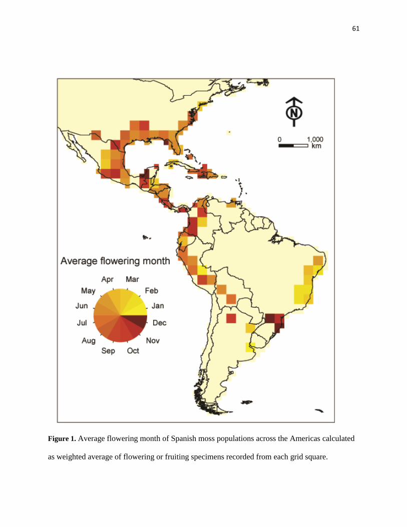
61
Figure 1. Average flowering month of Spanish moss populations across the Americas calculated
as weighted average of flowering or fruiting specimens recorded from each grid square.
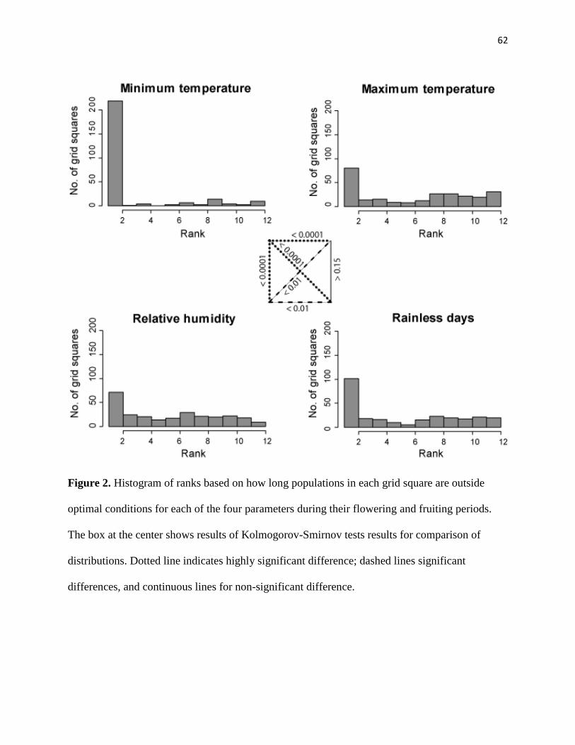
62
Figure 2. Histogram of ranks based on how long populations in each grid square are outside
optimal conditions for each of the four parameters during their flowering and fruiting periods.
The box at the center shows results of Kolmogorov-Smirnov tests results for comparison of
distributions. Dotted line indicates highly significant difference; dashed lines significant
differences, and continuous lines for non-significant difference.

63
Figure 3. Optimal flowering and fruiting month for Spanish moss populations based on each
physiological parameter in isolation.

64
Figure 4. Map of Euclidean distances from observed conditions for Spanish moss populations to
the best available across the species’ distribution. Inset shows a frequency histogram of distances
in grid squares (top) and relationship to numbers of specimens on which distance calculations
were based (bottom).

65
Chapter 3
Physiological thermal maxima and impact of
warming climates across the geographic
distributions of 33 anuran species

66
Abstract
Species populations are affected by diverse aspects of weather and climate when variation takes
conditions out of normal tolerance ranges; particularly of concern may be increases in
temperature. Projected mean temperature increases may induce increases in extreme values
which can be detrimental for many populations, as it will often not be possible to adapt to these
changes. Amphibians are particularly affected by climate change owing to their small body size
and ectothermic physiology: critical maximum temperature CTmax is an important element at the
larval stage. We use experimentally measured CTmax values for 33 anuran species and 6-hourly
resolution ERA weather data from 1989-2010 to understand in which populations of each species
may experience CTmax and be under physiological stress. We also explored how frequently
CTmax has been reached, and whether that frequency is increasing. Our results indicate that about
70% of the species have experienced CTmax at least for a single day during the last 22-year period
somewhere in their ranges, but only one species experienced CTmax often during the 22-year time
period.

67
Introduction
Global warming and climate change more generally are causing significant changes in species’
geographic distributions. Many studies have demonstrated that species’ ranges are shifting
polewards owing to effects of warming temperatures (Root et al. 2003; Burrows et al. 2011;
Chen et al. 2011). The temperature increase of 0.6°C to date has not only already affected
species’ distributions, but has also affected parameters of ecosystem function and timing of
biological processes (Visser & Both 2005; Garrett et al. 2006). The projected change of
temperature increase of 2.5°C over the next 100 years is anticipated to manifest significant
changes in frequency of extreme climatic events, which will further affect species, and also may
even cause extinctions (Wake & Vredenburg 2008; Moritz & Agudo 2013). Numerous research
efforts have attempted to anticipate changes in distributions under future climatic scenarios using
correlative, niche-based approaches (Pearson & Dawson 2003; Zurell et al. 2009; Poulos et al.
2012). In the few studies to date, correlative and mechanistic approaches have yielded similar
predictions for species’ distributions under future climatic conditions (Buckley 2008; Kearney et
al. 2009, 2010). In this regard, it is essential to link geographic patterns of species’ distributions
to known physiological tolerances of species to evaluate the impacts of the rapidly changing
climate.
Even though most species are experiencing climate change amphibians are particularly affected
as a whole, and are experiencing a large-scale declines, which are at least partly climate-driven
(Stuart et al. 2003; Wake 2006). An estimated 43% of amphibian species are declining (Stuart et
al. 2003); indeed, 32% of the species are threatened with extinction, and this period could be
considered a mass extinction event (Wake & Vredenburg 2008). Four major factors affecting

68
amphibian populations include climate change, environmental pollutants, habitat modification,
and invasive species and pathogens (Hayes et al. 2010). Considering climate warming,
amphibian populations may frequently be exposed to conditions close to critical maximum
temperatures tolerance limits, and their ability to adapt to temperature increases may be limited
(Huey & Berrigan 2001; Hayes et al. 2010; Burrows et al. 2011). In this regard, identifying
species and populations living at sites manifesting conditions close to critical maximum
temperatures and potentially causing physiological stress becomes crucial.
For anuran species, critical maximum temperature (CTmax) in larval stages represents an
important constraint in life cycles. An individual experiencing conditions approaching CTmax has
higher chances of death or abnormal larval development, which in turn is reflected in declining
recruitment to reproductive populations (Benard 2015). Little research has been done in regard to
how often species experience CTmax temperatures in real life, or whether the frequency of
exposure to CTmax is increasing over time as a consequence of climate change. Hence, this
contribution, we use high-temporal-resolution climatic data to understand what parts of species’
distributions experience conditions approaching CTmax and whether species have been
experiencing CTmax increasingly frequently over the past two decades.
Methods
Species Data
Durate et al. (2012) studied 47 amphibian species at 3 locations presenting varied environmental
conditions; we focus on the 41 anuran species included in that study. Study sites included (1) the
Gran Chaco region of northern Argentina (23.8°–27.5°S), which has a warm subtropical climate;

69
(2) the Atlantic Forest biome of Misiones Province in northeastern Argentina (27.5°–27.1°S),
with cooler subtropical environmental conditions; and (c) the Iberian Peninsula of Europe
(36.9°–60.5°N), with cool temperate conditions. Duarte et al. (2012) derived critical maximum
temperatures for each species following Hutchinson’s dynamic method. In this method, the
endpoint is determined by onset of muscular spasms after heating the individual at a constant
heating rate of 1°C min-1
(Hutchison 1961). (Details of parameters and procedures are in (Duarte
et al. 2012).
Of the initial 41 species, we discarded those species with areas of <10 1.5° grid squares, (about
1650 x 1650 km2), leaving 33 species for analysis (Table 1), for each of which the original study
had measured CTmax. We collected breeding season information for each species from the
literature and from AmphibiaWeb (2015 (www.amphibiaweb.org; Table 1). In two cases, lacking
breeding season information, we used the collection periods given in Duarte et al. (2012) as
breeding period, in absence of more detailed information.
We downloaded crude summaries of geographic distributions of each species from the Global
Amphibian Assessment (http://www.iucnredlist.org/initiatives/amphibians; IUCN, (2009) This
dataset was developed by herpetologists from their expert knowledge and provides a rough
distributional summary for each species. We buffered the IUCN distributional polygon by 80
km, to identify the set of grid squares that cover the entire distributional area for each species.
We also downloaded occurrence data for each species from GBIF (www.gbif.org) and HerpNET
(www.herpnet.org). Records of each species were assessed for inconsistencies such as (1) place
name and geographic coordinates do not match; (2) geographic coordinates fall in the ocean or

70
on a different continent; and (3) duplicate records. These data were corrected where possible, and
otherwise deleted from analysis (Chapman 2005).
Climate Data
We examined how the maximum thermal temperature (CTmax) was or was not met for each
species across its geographic distribution during the breeding season over a 22-year period
(January 1989 – December 2010). To this end, we used the ERA Interim Reanalysis Climate
Data developed and supplied by the European Center for Medium-Range Weather Forecasts.
These data are based on a combination of models and observations, with 3-hourly temporal
resolution: every second datum is a forecast, whereas the other is a model result. We used only
the model result data, thus coarsening the data from 3-hourly to 6-hourly temporal resolution.
The dataset has a somewhat coarse native spatial resolution of 1.5° x 1.5°, or approximately 165
x 165 km grid square resolution at the Equator.
ERA data were downloaded from http://apps.ecmwf.int/datasets/data/interim_full_daily/ for
maximum temperature at 2 m above the ground. The ERA data are stored in NetCDF format
(http://www.unidata.ucar.edu/packages/netcdf/index.html; Rew & Davis 1990); these data were
manipulated and processed via the “ncdf” package in R (Pierce 2011; R Core Development
Team, 2012
Data Analysis
An R script was developed using the raster, ncdf, and sp packages (Bivand et al. 2008; Pierce
2011; Hijmans & van Etten 2012) to calculate the number of days above CTmax in each breeding

71
season for each species over the 22-year span of the climate data set. The script checked the
value of maximum temperature across four daily observations; a grid square was marked as
“unsuitable” for a day whenever two consecutive observations were at or above the temperature
limit. It also calculated maximum number of days in sequence outside physiological tolerance
limits for each grid square in the distribution of each species. Maximum number of days outside
the physiological niche for each grid square was stored for every breeding season.
Using this information, we developed maps in which each grid square across the distribution is
marked as unsuitable whenever a grid square is outside the physiological tolerance limit on at
least one day, during any breeding season over the 22-year period. We calculated the proportion
of the distributional area of each species outside the physiological niche. We overlaid the curated
occurrence data (see above) on distributional maps and calculated proportions of occurrence
points falling outside species’ distribution areas (i.e data problem), and proportion of
occurrences falling outside the physiological niche but within the distributional area.
We calculated, for each species in each year, the maximum temperature within the distribution
area, maximum number of days in the distributional area above CTmax, and maximum number of
grid squares above CTmax. For each species, we developed a linear regression model assessing
the number of days outside the physiological niche, and the number of grid squares outside the
physiological niche as a function of time.

72
Results
Our analysis indicates that CTmax conditions have been experienced in at least one grid square
during the breeding season by 23 (70%) of the 33 anuran species. For nine species, the number
of grid squares going out of the physiological niche increased during the 22 years of this study.
Among the 33 species analyzed, species’ ranges covered 16–800 grid squares (Figure 1a). Figure
1(b) shows a summary of relationships between extent of distributional area and the proportion
of the distribution experiencing CTmax for each of 33 anuran species during the 22 years. The
maximum proportion of distribution area outside the physiological niche is for the species
Ceratophrys cranwelli, which does not have particularly large distribution. The species with the
largest distribution was Bufo bufo; 90% of the distributional area of this species was within the
physiological niche limits for the entire study period. For ten species, none of the distributional
area manifested temperatures was outside the physiological niche during the study period.
Distributional areas within and outside the physiological niche are shown for four example
species in Figure 2 (see also Supplementary Figure 2). For example, Bufo bufo (Figure 2c) has a
broad distribution, and only a few peripheral grid squares were outside of the physiological
niche. For Alytes cisternasii, no part of the distribution experienced critical maximum
temperature on any day during the 22-year study period. In contrast, major parts of the
distribution of Ceratophrys cranwelli experienced CTmax on at least one day in the 22-year
period. Distributional summaries were coarse in nature, but in many cases the actual occurrence
data fell outside tolerance limits. Occurrence data at sites manifesting conditions outside the
physiological niche limits ranged 1-42% (Figure 3). For Rhinella ornata, no data were available
on GBIF or HerpNet, as this species is vulnerable; none of the species had all occurrence data

73
falling within the IUCN distribution outline. For Phyllomedusa sauvagii, most of the occurrences
fell under low–suitability physiological conditions. However, for Leptodactylus bufonius and
Lepidobatrachus llanensis, even though the distributional area contained grid squares with low
physiological suitability, known occurrences did not fell in those areas.
Temporal trends in frequency of experiencing CTmax from year to year are summarized in Figure
4. For Bufo bufo, the number of grid squares experiencing CTmax increased significantly over the
study period (R2 = 0.26, P < 0.02). For Scinax fuscovarius, the number of consecutive days
above CTmax and number of grid squares experiencing CTmax increased within the distribution
(Figure 4b, Supplementary Figure 1). Overall, however, of the 33 anuran species analyzed, only
Bufo bufo showed significant (P <0.05) temporal trends (Table 2).
Discussion
Physiological tolerance limits can be informative in understanding geographic distributions and
range limits of species, and may be particularly relevant in climate change scenarios (Porter et al.
2000; Pörtner & Farrell 2008). To understand how species may shift their geographic
distributions, the frequency of exceptions to physiological tolerances can be projected on to
geography. This approach is potentially important but has been implemented only for few
ectothermic species (Kleidon & Harold 2000; Kearney & Porter 2004; Kearney et al. 2008;
Buckley 2008; Helmuth 2009; Buckley et al. 2010). The correlational analog technique is to
infer physiological limits from the occupied geographic distribution (Peterson 2001; Soberón &
Peterson 2005; Elith & Leathwick 2009; La Sorte & Jetz 2010; Poulos et al. 2012; Bentlage et
74
al. 2013); this latter technique has become much more popular owing to ease of operation and
convenient data availability.
Physiological parameters are not available for most species, owing to time and cost constraints
involved with obtaining estimates of key parameter values. However, when such data are
available, they can be highly informative about how climate change may affect species’
distributions. We used CTmax estimates for 33 anuran species to understand which species will
prove more vulnerable in light of warming climates, and how much of each species’ distribution
is under unsuitable conditions in terms of maximum temperature. In overview, about 70% of the
species experienced CTmax conditions during 22 years in at least part of their geographic
distributions (Figures 1, 4). For only one species, the number of days with CTmax and proportion
of the distribution experiencing CTmax increased dramatically and significantly over the study
period.
Duarte et al (2012) explored differences between the CTmax and maximum pond temperatures
(Tmax) at three different localities with different environmental conditions. Their result suggests
that the difference between CTmax and Tmax is less in subtropical warm locations, such that
species in subtropical warm locations may have more narrow tolerances. Our results also
supported this idea: species in subtropical locations appeared to experience CTmax more
frequently than species in temperate regions. For some temperate species, the peripheral parts of
the distribution were frequently outside of the physiological niche, such that populations in those
regions may be more physiologically stressed.
75
We observed that these phenomenon of distributional areas outside of the physiological niche
was particularly frequent at lower latitudes are from lower latitudes (Figure 2, Supplementary
Figure 2) which may have particularly serious implications for these species’ geographic ranges.
Besides anurans, many marine invertebrates and lizards are believed threatened by increases in
temperatures, as they appear to live close to their thermal tolerance limits (Sinervo et al. 2010;
Somero 2010). A few case studies suggest that species cannot adapt fast enough to keep up with
warming climate (Hoffmann & Sgrò 2011), a few recent studies (Logan et al. 2014; Ferri-Yáñez
& Araújo 2015) have demonstrated temperature adaptation in species of lizards with strong
natural selection favoring individuals who could run faster in warmer environments. Whether
similar process is happening or could happen in anuran species, or how targets of selection may
differ, is not yet known.
One concern about this study’s design is that the distributional areas used in this study (IUCN
2009) are rather crude, such that our estimates or physiological stress across distribution areas
may be rather noisy. For almost all (95%) of the species, we found that many populations occur
outside the IUCN distribution region (and we checked taxanomic concepts carefully to avoid
artifacts). It is important to validate these occurrences or update the distributional summaries, to
make estimates of threat under climate change scenario more accurate. For example, for species
Pseudis platensis more than 50% of available occurrences fell outside the IUCN distributional
border. We could not validate the IUCN distributional area for species Rhinella ornata as no
occurrences are available; as this species is considered vulnerable, geo-locations have not been
made public.

76
Overall, our analysis revealed that, among 33 species of anurans, some part of the distributional
areas for 23 of the species experienced CTmax during a 22-year time period. However, our
analysis of temporal trends during the 22-year time span showed only a single significant result.
Only Bufo bufo showed that number of days experiencing CTmax , and number of pixels
experiencing CTmax had increased. Using our approach, we could not conclude that climate
change has already been affecting these species’ distributional areas significantly.
Acknowledgements
We thank Dr. Varad Giri, Dr. Krushnamegh Kunte and Vijay Barve for insightful discussion. Dr.
Nathaniel Brunsell for help with ERA data.
References
Almeida CP de, Uetanabaro M, Lopes FS, Journal S, Mar N (2015) Reproductive strategies of
Leptodactylus chaquensis and L. podicipinus in the Pantanal, Brazil. Journal of
Herpetology, 34, 135–139.
AmphibiaWeb: Information on amphibian biology and conservation. (Web application). (2015)
Berkeley, California: AmphibiaWeb. Available: http://amphibiaweb.org/. (accessed:Apr 16,
2015)
Benard MF (2015) Warmer winters reduce frog fecundity and shift breeding phenology, which
consequently alters larval development and metamorphic timing. Global Change Biology,
21, 1058–1065.
77
Bentlage B, Peterson AT, Barve N, Cartwright P (2013) Plumbing the depths: extending
ecological niche modelling and species distribution modelling in three dimensions. Global
Ecology and Biogeography, 22, 952–961.
Bivand RS, Pebesma EJ, Gómez-Rubio V (2008) Applied spatial data analysis with R. New
York, Springer.
Both C, Kaefer ÍL, Santos TG, Cechin STZ (2008) An austral anuran assemblage in the
Neotropics: seasonal occurrence correlated with photoperiod. Journal of Natural History,
42, 205–222.
Buckley LB (2008) Linking traits to energetics and population dynamics to predict lizard ranges
in changing environments. American Naturalist, 171, E1–E19.
Buckley LB, Urban MC, Angilletta MJ, Crozier LG, Rissler LJ, Sears MW (2010) Can
mechanism inform species’ distribution models? Ecology Letters, 13, 1041–1054.
Burrows MT, Schoeman DS, Buckley LB, et al. (2011) The pace of shifting climate in marine
and terrestrial ecosystems. Science, 334, 652–655.
Cei JM (1968) Notes on the tadpoles and breeding ecology of Lepidobatrachus (Amphibia:
Ceratophryidae). Herpetologica, 24, 141–146.
Chapman AD (2005) Principles and methods of data cleaning—primary species and species-
occurrence data. Global Biodiversity Information Facility, Copenhagen.
Chen I, Hill JK, Ohlemüller R, Roy DB, Thomas CD (2011) Rapid range shifts of species
associated with high levels of climate warming. Science, 333, 1024–1027.
Dias TM, Maragno FP, Madalozzo B, Prado CPA, Cechin SZ (2013) Breeding sites of the leaf
frog Phyllomendusa tetraploidea (Hylidae, Phyllomedusinae) in a forest remnant in
southern Brazil. North-western Journal of Zoology, 9, 422–424.

78
Diaz-Paniagua C (1988) Temporal segregation in larval amphibian communities in temporary
ponds at a locality in SW Spain. Amphibia-Reptilia, 9, 15–26.
Duarte H, Tejedo M, Katzenberger M, et al. (2012) Can amphibians take the heat? Vulnerability
to climate warming in subtropical and temperate larval amphibian communities. Global
Change Biology, 18, 412–421.
Elith J, Leathwick JR (2009) Species distribution models: ecological explanation and prediction
across space and time. Annual Review of Ecology, Evolution, and Systematics, 40, 677–697.
Ferri-Yáñez F, Araújo MB (2015) Lizards could be warming faster than climate. Ecography, 38,
1–3.
Friedl TWP, Klump GM (1997) Some aspects of population biology in the European Treefrog.
Hyla arborea. Herpetologica, 53, 321–330.
Froglife National wildlife conservation charity. (Web application). (2015) Peterborough,
London: Available: http://www.froglife.org/. (accessed:Apr 16, 2015)
Garrett KA, Dendy SP, Frank EE, Rouse MN, Travers SE (2006) Climate change effects on
plant disease: genomes to ecosystems. Annual Review of Phytopathology, 44, 489–509.
Gómez-Rodríguez C, Díaz-Paniagua C, Serrano L, Florencio M, Portheault A (2009)
Mediterranean temporary ponds as amphibian breeding habitats: the importance of
preserving pond networks. Aquatic Ecology, 43, 1179–1191.
Haddad C, Uetanabaro M, Prado CP de A (2005) Breeding activity patterns, reproductive modes,
and habitat use by anurans (Amphibia) in a seasonal environment in the Pantanal, Brazil.
Amphibia-Reptilia, 26, 211–221.

79
Hayes TB, Falso P, Gallipeau S, Stice M (2010) The cause of global amphibian declines: a
developmental endocrinologist’s perspective. Journal of Experimental Biology, 213, 921–
933.
Helmuth B (2009) From cells to coastlines: how can we use physiology to forecast the impacts of
climate change? Journal of Experimental Biology, 212, 753–760.
Heyer RW, Bellin MS (1973) Ecological notes on five sympatric Leptodactylus (Amphibia,
Leptodactylidae) from Ecuador. Herpetologica, 29, 66–72.
Hijmans RJ, van Etten J (2012) raster: Geographic analysis and modeling with raster data.
Hoffmann AA, Sgrò CM (2011) Climate change and evolutionary adaptation. Nature, 470, 479–
485.
Huey RB, Berrigan D (2001) Temperature, demography, and ectotherm fitness. American
Naturalist, 158, 204–210.
Hutchison VH (1961) Critical thermal maxima in salamanders. Physiological Zoology, 34, 92–
125.
IUCN (2009) Global amphibian assessment. Conservation International, Washington, DC,.
Journal S (2003) Testes size in leptodactylid frogs and occurrence of multimale spawning in the
genus Leptodactylus in Brazil. Journal of Herpetology, 37, 354–362.
Kearney M, Phillips BL, Tracy CR, Christian KA, Betts G, Porter WP (2008) Modelling species
distributions without using species distributions: the cane toad in Australia under current
and future climates. Ecography, 31, 423–434.
Kearney M, Porter WP (2004) Mapping the fundamental niche: physiology, climate, and the
distribution of a nocturnal lizard. Ecology, 85, 3119–3131.
80
Kearney M, Porter WP, Williams C, Ritchie S, Hoffmann AA (2009) Integrating biophysical
models and evolutionary theory to predict climatic impacts on species’ ranges: the dengue
mosquito Aedes aegypti in Australia. Functional Ecology, 23, 528–538.
Kearney MR, Wintle BA, Porter WP (2010) Correlative and mechanistic models of species
distribution provide congruent forecasts under climate change. Conservation Letters, 3,
203–213.
Kleidon A, Harold M (2000) A global distribution of biodiversity inferred from climatic
constraints: results from a process-based modelling study. Global Change Biology, 6, 507–
523.
Logan ML, Cox RM, Calsbeek R (2014) Natural selection on thermal performance in a novel
thermal environment. Proceedings of the National Academy of Sciences, 111, 14165–14169.
Moritz C, Agudo R (2013) The future of species under climate change: resilience or decline?
Science, 341, 504–509.
Pearson RG, Dawson TP (2003) Predicting the impacts of climate change on the distribution of
species: are bioclimate envelope models useful? Global Ecology and Biogeography, 12,
361–371.
Peltzer PM, Lajmanovich RC, Sánchez-Hernandez JC, Cabagna MC, Attademo AM, Bassó A
(2008) Effects of agricultural pond eutrophication on survival and health status of Scinax
nasicus tadpoles. Ecotoxicology and Environmental Safety, 70, 185–197.
Peterson AT (2001) Predicting species’ geographic distributions based on ecological niche
modeing. Condor, 103, 599–605.
Pierce D (2011) ncdf: interface to Unidata netCDF data files. Available at: http://CRAN.R-
project.org/package=ncdf (accessed 10 January 2014)

81
Porter WP, Srinivas; B, E. SW, Navin R (2000) Calculating climate effects on birds and
mammals: impacts on biodiversity, conservation, population parameters, and global
community structure. American Zoologist, 40, 597–630.
Pörtner HO, Farrell AP (2008) Physiology and climate change. Science, 322, 690–692.
Poulos HM, Chernoff B, Fuller PL, Butman D (2012) Mapping the potential distribution of the
invasive red shiner, Cyprinella lutrensis (Teleostei: Cyprinidae) across waterways of the
conterminous United States. Aquatic Invasions, 7, 377–385.
R Core Development Team (2012) R: A language and environment for statistical computing. R
Foundation for Statistical Computing, Vienna.
Rew R, Davis G (1990) NetCDF: An interface for scientific data access. IEEE Computer
Graphics and Applications, 10, 76–82.
Rodrigues DDJ, Lopes FS, Uetanabaro M (2003) Reproductive pattern of Elachistocleis bicolor
(Anura, Microhylidae) at Serra da Bodoquena, Mato Grosso do Sul, Brazil. Iheringia, Série
Zoologia, 93, 365–371.
Rodrigues D de J, Uetanabaro M, Lopes FS (2004) Reproductive strategies of Physalaemus
nattereri (Steindachner, 1863 ) and P . albonotatus (Steindachner, 1864 ) at Serra da
Bodoquena, State of Mato Grosso do Sul, Brazil. Revista Espanola de Herpetologia, 18,
63–73.
Root TL, Price JT, Hall KR, Schneider SH, Rosenzweig C, Pounds JA (2003) Fingerprints of
global warming on wild animals and plants. Nature, 421, 57–60.
Sinervo B, Mendez de la Cruz F, Miles DB, et al. (2010) Erosion of lizard diversity by climate
change and altered thermal niches. Science, 238, 894–899.

82
Soberón J, Peterson AT (2005) Interpretation of models of fundamental ecological niches and
species distributional areas. Biodiversity Informatics, 2, 1–10.
Somero GN (2010) The physiology of climate change: how potentials for acclimatization and
genetic adaptation will determine “winners” and “losers.” Journal of Experimental Biology,
213, 912–920.
La Sorte FA, Jetz W (2010) Avian distributions under climate change: towards improved
projections. Journal of Experimental Biology, 213, 862–869.
South S, Journal A (2011) Spatio-temporal distribution of calling male frogs in Morro do Diabo
State Park (southeastern Brazil): implication for conservation and management in a
seasonally dry tropical forest. South American Journal of Herpetology, 6, 107–118.
Stuart SN, Chanson JS, Cox NA, Young BE, Rodrigues ASL, Fischman DL, Waller RW (2003)
Status and trends of amphibian declines and extinctions worldwide. Science, 306, 1783–
1786.
Tejedo M (1993) Size-dependent vulnuerability and behavioral responses of tadpoles of two
anuran species to beetle larvae predators. Herpetologists’ League, 49, 287–294.
Toledo LF, Garey M V., Costa TRN, Lourenço de Moraes R, Hartmann MT, Haddad CFB
(2012) Alternative reproductive modes of Atlantic forest frogs. Journal of Ethology, 30,
331–336.
Visser ME, Both C (2005) Shifts in phenology due to global climate change: the need for a
yardstick. Proceedings of Royal Society B, 272, 2561–2569.
Wake DB (2006) Problems with species: patterns and processes of species formation in
salamanders. Annals of the Missouri Botanical Garden, 93, 8–23.

83
Wake DB, Vredenburg VT (2008) Are we in the midst of the sixth mass extinction? A view from
the world of amphibians. Proceedings of the National Academy of Sciences, 105, 11466–
11473.
Wogel H, Abrunhosa PA, Pombal Jr JP (2005) Breeding behaviour and mating success of
Phyllomedusa rohdei (Anura, Hylidae) in southeastern Brazil. Journal of Natural History,
39, 2035–2045.
Zurell D, Jeltsch F, Dormann CF, Schröder B (2009) Static species distribution models in
dynamically changing systems: how good can predictions really be? Ecography, 32, 733–
744.
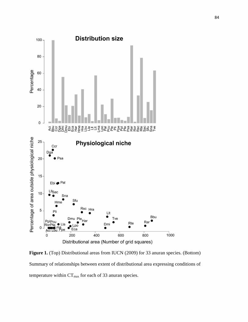
84
Figure 1. (Top) Distributional areas from IUCN (2009) for 33 anuran species. (Bottom)
Summary of relationships between extent of distributional area expressing conditions of
temperature within CTmax for each of 33 anuran species.
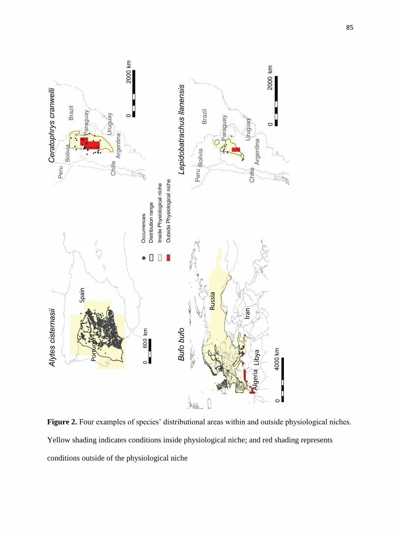
85
Figure 2. Four examples of species’ distributional areas within and outside physiological niches.
Yellow shading indicates conditions inside physiological niche; and red shading represents
conditions outside of the physiological niche
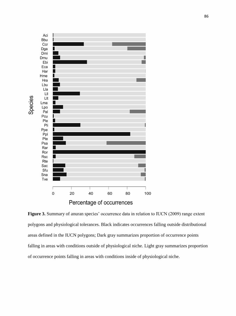
86
Figure 3. Summary of anuran species’ occurrence data in relation to IUCN (2009) range extent
polygons and physiological tolerances. Black indicates occurrences falling outside distributional
areas defined in the IUCN polygons; Dark gray summarizes proportion of occurrence points
falling in areas with conditions outside of physiological niche. Light gray summarizes proportion
of occurrence points falling in areas with conditions inside of physiological niche.

87
Figure 4. Summary of temporal trends for two example species. (Left): Number of days outside
physiological niche (dark gray), number of grid squares outside physiological niche (light gray)
(Middle): Relationship of number of days outside physiological niche and breeding year. (Right):
Relationship of number of grid squares outside physiological niche in distributional areas and
breeding year.

88
Table 1: List of anuran species with its respective CTmax and breeding seasons
Name Code CTmax in
(C)
Community Breeding season
Alytes cisternasii Aci 38.2 ± 0.2 Temperate September – March
(AmphibiaWeb, 2015)
Bufo bufo Bbu 38.3 ± 0.1 Temperate March – June (AmphibiaWeb,
2015)
Ceratophrys cranwelli Ccr 42.0 ± 0.1 Subtropical
warm
November – February (Duarte
et al. 2012)
Discoglossus galganoi Dga 38.4 ± 0.1 Temperate October – July
(AmphibiaWeb, 2015)
Dendropsophus minutus Dmi 40.6 ± 0.1 Subtropical
cool
September – February
(AmphibiaWeb, 2015)
Dermatonotus muelleri Dmu 43.6 ± 0.3 Subtropical
warm
September – February
(AmphibiaWeb, 2015)
Elachistocleis bicolor Ebi 41.7 ± 0.2 Subtropical
warm
September – March
(Rodrigues et al. 2003)
Epidalea calamita Eca 39.7 ± 0.1 Temperate September – May (“Froglife”)
Hyla arborea Har 40.0 ± 0.1 Temperate April – July (Friedl & Klump
1997)
Hyla meridionalis Hme 39.8 ± 0.1 Temperate March –June (Diaz-Paniagua
1988)
Hypsiboas raniceps Hra 41.2 ± 0.2 Subtropical
warm
September – March (Haddad
et al. 2005)
Leptodactylus bufonius Lbu 43.3 ± 0.1 Subtropical
warm
December (Heyer & Bellin
1973)
Leptodactylus latinasus Lla 44.7 ± 0.2 Subtropical
warm
September – May (Diaz-
Paniagua 1988)
Lepidobatrachus
llanensis
Lll 44.7 ± 0.2 Subtropical
warm
October – February (Cei
1968)
Leptodactylus latrans Llt 41.4 ± 0.2 Subtropical
warm
September – February
(AmphibiaWeb, 2015)
Limnomedusa
macroglossa
Lma 39.9 ± 0.2 Subtropical
cool
November – January (Both et
al. 2008)
Leptodactylus
podicipinus
Lpo 43.3 ± 0.3 Subtropical
cool
November – March (Almeida
et al. 2015)
Physalaemus albonotatus Pal 41.1 ± 0.2 Subtropical
warm
September –
March(Rodrigues et al. 2004)
Pelobates cultripes Pcu 39.4 ± 0.1 Temperate October – May (Tejedo 1993)
Pelophylax lessonae Ple 38.6 ± 0.2 Temperate May – July (AmphibiaWeb,
2015)
Pseudis limellum Pli 41.9 ± 0.1 Subtropical
warm
August – March
Pelophylax perezi Ppe 39.6 ± 0.2 Temperate February – June(Gómez-
Rodríguez et al. 2009)

89
Pseudis platensis Ppl 42.3 ± 0.1 Subtropical
warm
November – April (South &
Journal 2011)
Phyllomedusa sauvagii Psa 42.1 ± 0.3 Subtropical
warm
October – February (Wogel et
al. 2005)
Phyllomedusa
tetraploidea
Pte 41.6 ± 0.2 Subtropical
cool
October – December (Dias et
al. 2013)
Rana arvalis Rar 35.8 ± 0.1 Temperate March – June (AmphibiaWeb,
2015)
Rhinella ornata Ror 40.7 ± 0.1 subtropical August – February (Toledo et
al. 2012)
Rhinella schneideri Rsc 42.5 ± 0.1 Subtropical
warm
October – April
(AmphibiaWeb, 2015)
Rana temporaria Rte 37.2 ± 0.1 Temperate March – June (AmphibiaWeb,
2015)
Scinax acuminatus Sac 43.0 ± 0.2 Subtropical
warm
October – March (Journal
2003)
Scinax fuscovarius Sfu 41.0 ± 0.3 Subtropical October – February
(AmphibiaWeb, 2015))
Scinax nasicus Sna 42.6 ± 0.2 Subtropical
warm
November – February (Peltzer
et al. 2008)
Trachycephalus
venulosus
Tve 41.9 ± 0.1 Subtropical
warm
November – February
(AmphibiaWeb, 2015))

90
Table 2: Summary of linear regression models assessing trends in maximum temperature as a
function of time across species’ distributions
Species
P
Number
of
days
Number of
grid squares
Alytes cisternasii - -
Bufo bufo 0.0195 0.0104
Ceratophrys cranwelli 0.1802 0.3531
Discoglossus galganoi 0.2274 0.2436
Dendropsophus minutus - -
Dermatonotus muelleri 0.0979 0.0979
Elachistocleis bicolor 0.1675 0.4123
Epidalea calamita - -
Hyla arborea 0.2185 0.2721
Hyla meridionalis 0.1047 0.2056
Hypsiboas raniceps 0.1875 0.4053
Leptodactylus bufonius - -
Leptodactylus latinasus 0.3517 0.7616
Lepidobatrachus
llanensis 0.0979 0.0979
Leptodactylus latrans 0.1777 0.3183
Limnomedusa
macroglossa - -
Leptodactylus
podicipinus 0.0979 0.0979
Physalaemus albonotatus 0.1384 0.2548
Pelobates cultripes - -
Pelophylax lessonae 0.2272 0.2272
Pseudis limellum 0.0979 0.0979
Pelophylax perezi - -
Pseudis platensis - -
Phyllomedusa sauvagii 0.1542 0.2107
Phyllomedusa
tetraploidea - -
Rana arvalis 0.9277 0.8067
Rhinella ornata - -
Rhinella schneideri 0.1513 0.1889
Rana temporaria 0.2272 0.2272
Scinax acuminatus 0.2091 0.2222
Scinax fuscovarius 0.1608 0.3505
Scinax nasicus 0.1731 0.212
Trachycephalus 0.1923 0.4625

91
venulosus
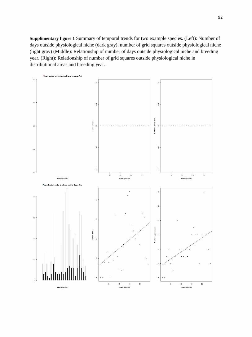
92
Supplimentary figure 1 Summary of temporal trends for two example species. (Left): Number of
days outside physiological niche (dark gray), number of grid squares outside physiological niche
(light gray) (Middle): Relationship of number of days outside physiological niche and breeding
year. (Right): Relationship of number of grid squares outside physiological niche in
distributional areas and breeding year.

93

94
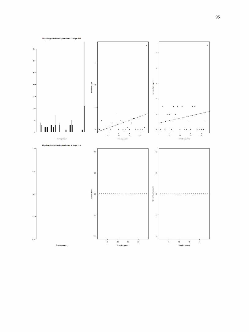
95

96

97
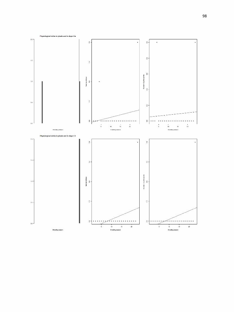
98

99

100

101
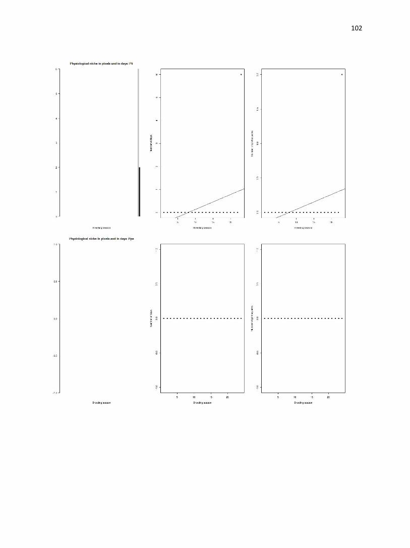
102
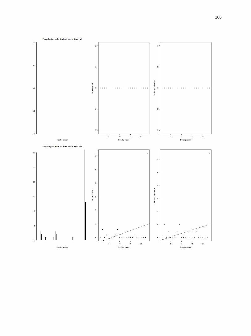
103

104

105
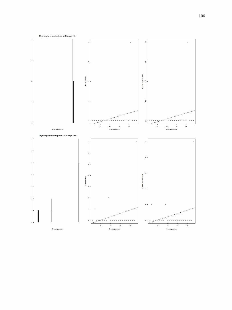
106
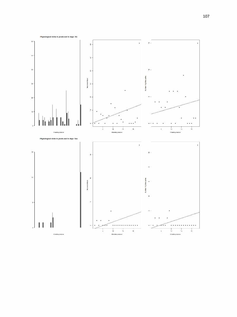
107

108

109
Supplimentary figure 2 Species’ distributional areas within and outside physiological niches.
Yellow shading indicates conditions inside physiological niche; and red shading represents
conditions outside of the physiological niche
Alytes cisternasii
Bufo bufo

110

111
Ceratophrys cranwelli
Discoglossus galganoi

112
Dendropsophus minutus
Dermatonotus muelleri
Elachistocleis bicolor

113
Epidalea calamita
Hyla arborea

114
Hyla meridionalis
Hypsiboas raniceps
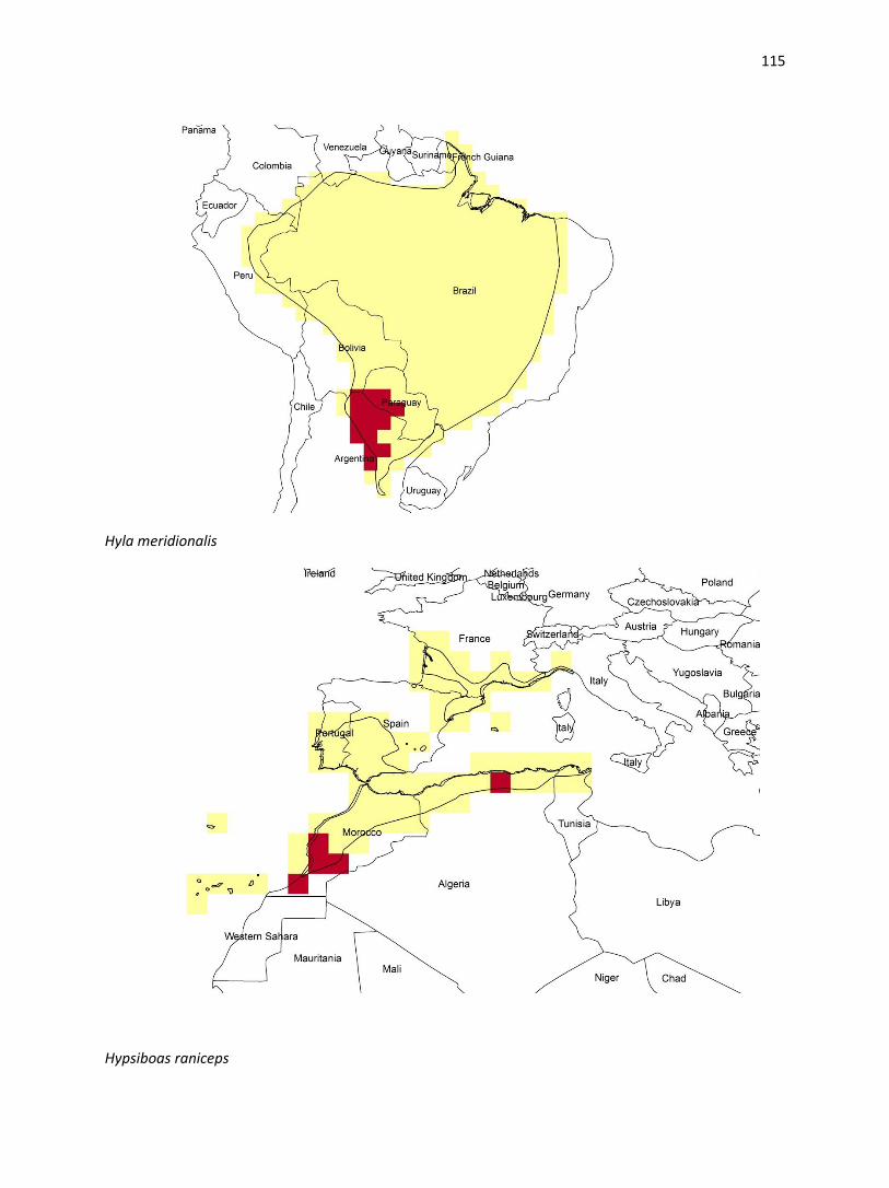
115
Hyla meridionalis
Hypsiboas raniceps

116
Leptodactylus bufonius
Leptodactylus latinasus
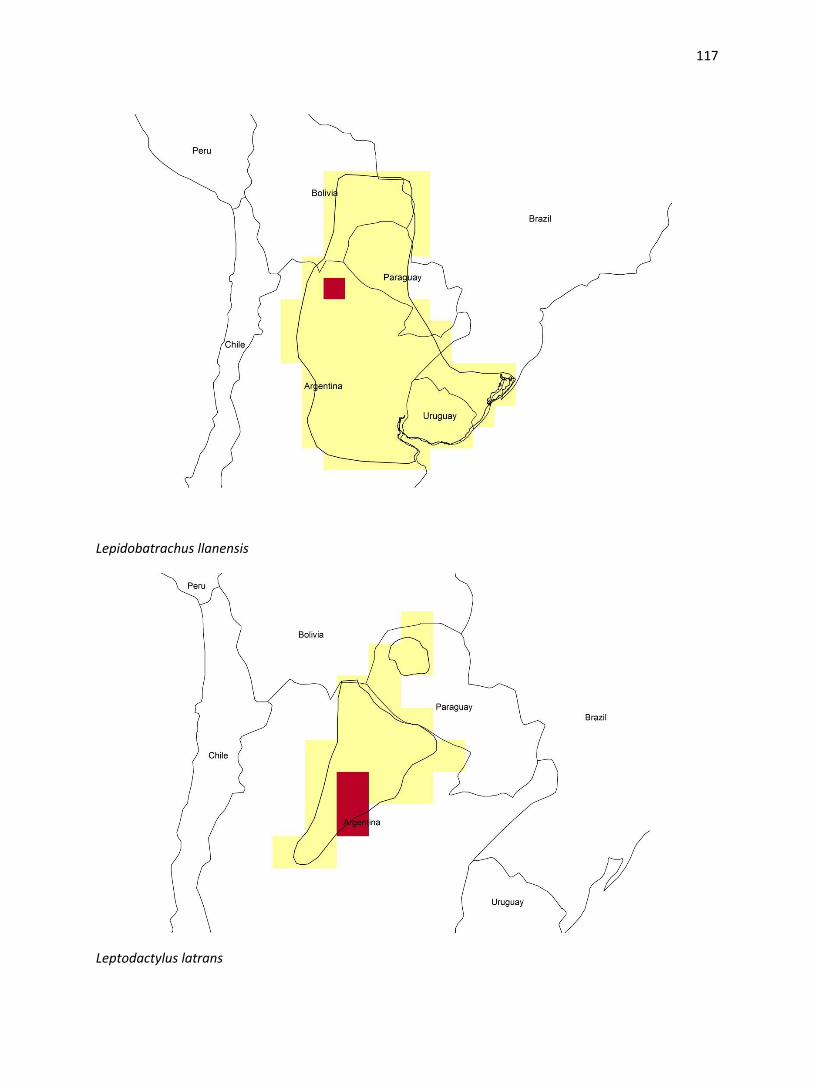
117
Lepidobatrachus llanensis
Leptodactylus latrans

118
Limnomedusa macroglossa
Leptodactylus podicipinus

119
Physalaemus albonotatus
Pelobates cultripes

120
Pelophylax lessonae
Pseudis limellum

121
Pelophylax perezi
Pseudis platensis

122
Phyllomedusa sauvagii
Phyllomedusa tetraploidea

123
Rana arvalis
Rhinella ornata

124
Rhinella schneideri
Rana temporaria
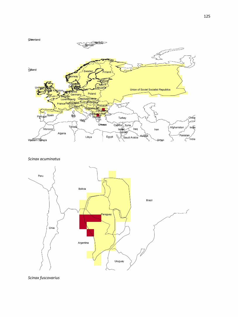
125
Scinax acuminatus
Scinax fuscovarius
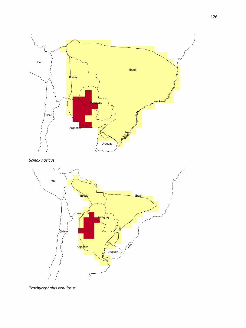
126
Scinax nasicus
Trachycephalus venulosus
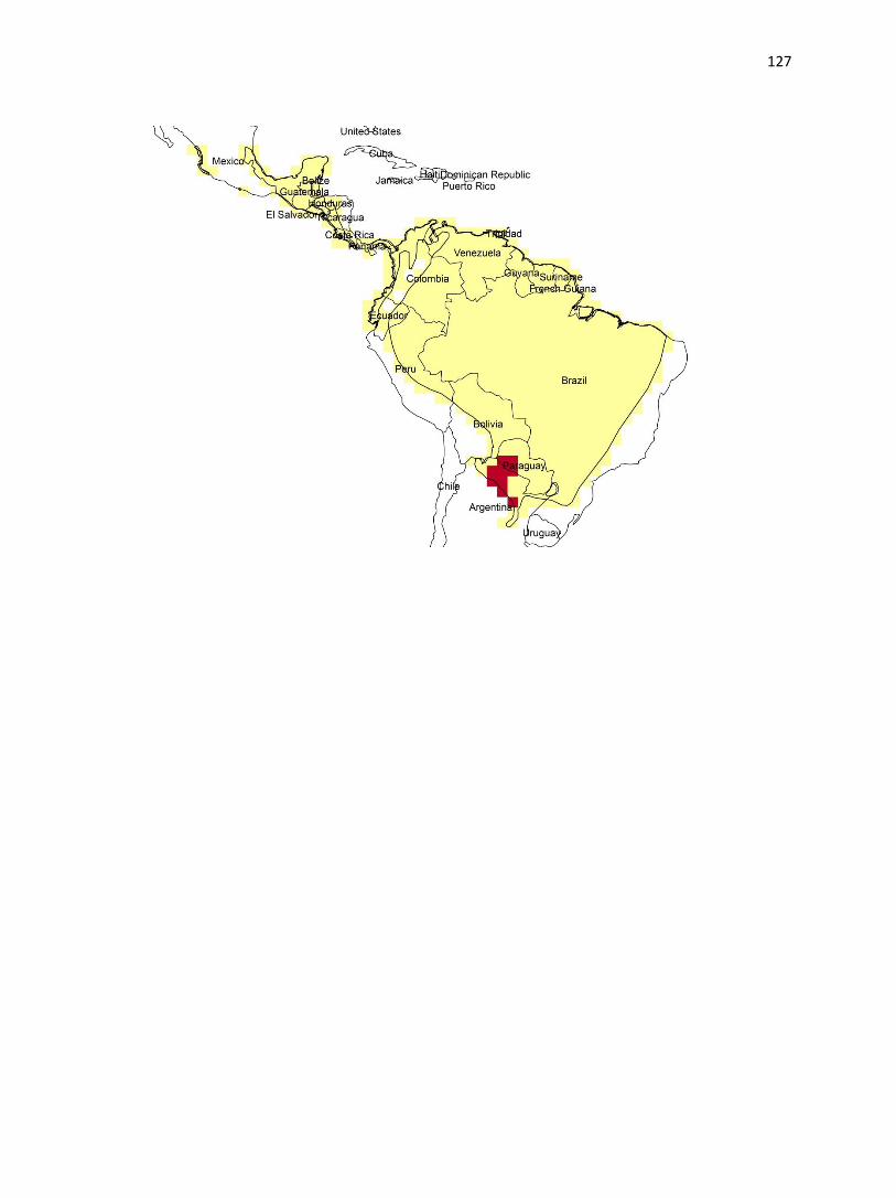
127