Physics of Fluids - · PDF filePhysics of Fluids J.Pearson May 26, 2009 Abstract These are a set of notes I have made, based on lectures given by T.Mullin at the Uni-versity of Manchester

Physics of Fluids

J.Pearson

May 26, 2009

Abstract

These are a set of notes I have made, based on lectures given by T.Mullin at the Uni-versity of Manchester Jan-May ’09. Please e-mail me with any comments/corrections:[email protected]. These notes may be found at www.jpoffline.com.

ii

CONTENTS iii

Contents

1 Introduction 1

1.1 Fluid as a Continuum . . . . . . . . . . . . . . . . . . . . . . . . . . . . . . . 1

1.1.1 Microscopic Level & The Continuum . . . . . . . . . . . . . . . . . . 2

2 Developing the Equations of Motion 5

2.1 Streamlines . . . . . . . . . . . . . . . . . . . . . . . . . . . . . . . . . . . . 5

2.1.1 Visualising & Measuring Flows . . . . . . . . . . . . . . . . . . . . . 5

2.2 The Navier-Stokes Equations . . . . . . . . . . . . . . . . . . . . . . . . . . . 6

2.2.1 The Material Derivative . . . . . . . . . . . . . . . . . . . . . . . . . 7

2.2.2 Developing the Navier-Stokes Equations . . . . . . . . . . . . . . . . 8

2.3 Scaling Navier-Stokes & Reynolds Number . . . . . . . . . . . . . . . . . . . 11

3 Exact Solutions 13

3.1 Unidirectional Flow Between Infinite Plates . . . . . . . . . . . . . . . . . . 13

3.2 Hagen-Poiseuille Flow . . . . . . . . . . . . . . . . . . . . . . . . . . . . . . 15

3.3 Flow Down Inclined Plane . . . . . . . . . . . . . . . . . . . . . . . . . . . . 17

3.4 Unsteady Flow . . . . . . . . . . . . . . . . . . . . . . . . . . . . . . . . . . 19

3.5 Steady Driven Flow With Inflow . . . . . . . . . . . . . . . . . . . . . . . . . 21

3.6 Low Reynolds Number Flow: Stokes Flow . . . . . . . . . . . . . . . . . . . 24

3.7 Stream Functions . . . . . . . . . . . . . . . . . . . . . . . . . . . . . . . . . 24

3.7.1 Stokes Flow Past a Sphere . . . . . . . . . . . . . . . . . . . . . . . . 26

3.8 Steady Inviscid Flows . . . . . . . . . . . . . . . . . . . . . . . . . . . . . . . 29

3.8.1 D’Alembert’s Paradox . . . . . . . . . . . . . . . . . . . . . . . . . . 30

3.8.2 Applications of Bernoulli’s Theorem . . . . . . . . . . . . . . . . . . . 31

4 Vorticity 35

4.1 Examples . . . . . . . . . . . . . . . . . . . . . . . . . . . . . . . . . . . . . 36

4.1.1 Irrotational Flow . . . . . . . . . . . . . . . . . . . . . . . . . . . . . 36

4.1.2 Solid Body Rotation . . . . . . . . . . . . . . . . . . . . . . . . . . . 36

iv CONTENTS

4.1.3 Hele-Shaw Flow . . . . . . . . . . . . . . . . . . . . . . . . . . . . . . 37

4.2 Irrotational Flow & The Complex Potential . . . . . . . . . . . . . . . . . . 38

4.2.1 Examples of w-flows . . . . . . . . . . . . . . . . . . . . . . . . . . . 39

5 Lubrication Theory 43

5.1 The Lubrication Equations . . . . . . . . . . . . . . . . . . . . . . . . . . . . 44

5.2 Slider Bearing . . . . . . . . . . . . . . . . . . . . . . . . . . . . . . . . . . . 45

5.2.1 Cavitation . . . . . . . . . . . . . . . . . . . . . . . . . . . . . . . . . 48

5.2.2 Adhesion . . . . . . . . . . . . . . . . . . . . . . . . . . . . . . . . . . 49

6 Aerofoil Theory 51

6.1 Circulation . . . . . . . . . . . . . . . . . . . . . . . . . . . . . . . . . . . . 52

6.2 The Magnus Effect . . . . . . . . . . . . . . . . . . . . . . . . . . . . . . . . 54

7 Boundary Layers 55

7.1 2D Boundary Layers . . . . . . . . . . . . . . . . . . . . . . . . . . . . . . . 56

8 Hydrodynamic Instability & Transition to Turbulence 61

8.1 Linear Stability . . . . . . . . . . . . . . . . . . . . . . . . . . . . . . . . . . 62

8.1.1 Hopf Bifurcation . . . . . . . . . . . . . . . . . . . . . . . . . . . . . 65

8.2 Landau Theory for Onset of Turbulence . . . . . . . . . . . . . . . . . . . . 66

8.3 Turbulence . . . . . . . . . . . . . . . . . . . . . . . . . . . . . . . . . . . . . 69

8.3.1 Energy Cascade . . . . . . . . . . . . . . . . . . . . . . . . . . . . . . 69

8.4 The Kolmogorov Spectrum . . . . . . . . . . . . . . . . . . . . . . . . . . . . 70

8.5 Reynolds Stresses . . . . . . . . . . . . . . . . . . . . . . . . . . . . . . . . . 71

1

1 Introduction

The aim of this is to discuss classical fluid dynamics, with some emphasis upon examples& applications. We shall vaguely derive most equations – but these derivations will not berigorous!

We seek some universality – typical behaviour from non-linear systems. In particular,how the onset of turbulence occurs in a system. Consider a system, whereby a smoothinput is taken by a system, which has non-linear deterministic equations of motion, andchaos is outputted. This chaotic output is still deterministic, and if the initial conditionsare known precisely (i.e. with no error at all), then this chaotic output will be entirelypredictable. However, that initial conditions are only known to a given accuracy, the outputwill always (practically) be unpredictable: chaos. A very simple example of such a system isthe undamped pendulum. Its full equation of motion is of the form

θ + sin θ = 0.

Now, this is a highly non-linear problem. The usual route for solving is to make the smallangle approximation (sin θ → θ), to give the easily soluble linear equation

θ + θ = 0.

So, for large initial amplitude (i.e. where the small angle approximation breaks down), theequations of motion are non-linear.

Another example is the Lorenz system, whereby the governing differential equations are

x = σ(x− y),

y = rx− y − xz,z = −bz + xy;

where σ, r are parameters. Such differential equations produce the so-called “Lorenz attrac-tor”, and the ideas behind them are able to model a variety of systems; such as weathermodeling.

Now, it is usually easy to write down the equations of motion of a non-linear system, butit is virtually impossible to solve them, even with modern supercomputers.

1.1 Fluid as a Continuum

We shall define that a fluid is some substance that moves under the action of a deformingforce, with true fluids having no rigidity (so that they are unable to support shear stressanywhere – shear stress vanishes everywhere).

2 1 INTRODUCTION

Not all materials which fall into the first category are fluids. For example, thixotropic andviscoelastic solids are not fluids (with examples being paint, jellies, toothpaste and putty,respectively). However, others are – examples being liquid glass and pitch/tar.

Flowing sand is “fluid-like”, but it can support shear stress in some circumstances. Considera grain silo, with a small open tube at the bottom, as in Figure (1.1). The pressure in the silois independent of depth (note that this is in contrast to water, whose pressure is dependentupon depth below the surface); and the rate of flow of the grain, through the tube is entirelydetermined by frictional effects at the tube (again, the rate of flow of water through such atube is dependent upon the amount of water above the tube). We will consider both liquids

Grain silo

of depthPressure independent

Figure 1.1: A grain silo: the pressure within the silo is independent of depth below the surface; thisis in complete contrast with a tub filled with water.

& gasses, as the dynamics of both is determined by the same set of equations.

1.1.1 Microscopic Level & The Continuum

Liquid molecules are in intimate contact with one another. Thus, if we shear such an object,molecules will realign in a very complicated manner. Gases, on the other hand, are composedof well separated molecules, whose mean free path is large.

Basically, fluids are very difficult (if not impossible) to treat at a microscopic level. So, toget around this, we introduce the hypothesis of a continuum.

We introduce “fluid elements” as being large enough to enclose many molecules, but smallenough to cope with large gradients. Hence, fluid dynamics is concerned with macroscopicflow phenomena.

The first of the requirements implies that average quantities are well defined – such astemperature, pressure, velocity, density.

1.1 Fluid as a Continuum 3

If we were to plot the dependance of the average density ρ within a cube of side a, we findthat at very small scales (≈ 10−10m), the average density is ill defined, with many “randomfluctuations (this is due to molecular fluctuations). On scales ≈ 10−7 → 10−4m, we see thatρ is approximately constant, and above 10−1m, either raise or drop. Now, the reasons behindraising or lowering is that the density changes due to large scale effects, such as temperaturechanges. The intermediate, roughly constant value of ρ is the local value, and is taken to bethe density.

Thus, the size of a (i.e. the size of the “fluid element”) should be ≈ 10−5m, in order thatthere is little variation in physical and dynamical properties within the element. Hence, aninstrument sensitive to (10−5m)

3= 10−15m−3 will measure a local value. For example, in

such a volume will be ≈ 1010 molecules of air.

Molecules can be exchanged between “fluid particles” by the diffusion process – via viscosity(in which case momentum will be transferred) or thermal conductivity (temperature). So,the size of the fluid particles must be greater than the mean free path of the molecules; thatis, molecules must suffer many collisions. The mean free path, of air molecules at STP is≈ 10−7m.

From hereon, the concept of a “point” in a fluid, and “fluid particle” are taken to be thesame.

We shall only consider incompressible Newtonian flows. Now, compressible effects are onlyimportant when the speed of the fluid exceeds the speed of sound in the fluid;

cairs ≈ 340ms−1, cwater

s ≈ 1400ms−1.

Hence, only for things like underwater explosions, or air passing over a jets wings, will wehave to consider compressible effects (which we shall not do here). Newtonian fluids arefluids for whom stress is proportional to strain, with the constant of proportionality beingthe molecular viscosity;

Newtonain fluid ⇒ stress = µ× strain.

For example, if a fluid element is subject to a strain of ∂u∂y

(i.e. moves along one edge), then

τ = µ∂u

∂y.

Most fluids are Newtonian, but a few examples that are non-Newtonian include polymersolutions (such as shower gel, shampoo etc) and liquid crystals (as found in laptop displayscreens).

4 1 INTRODUCTION

5

2 Developing the Equations of Motion

Here we shall present a rather heuristic derivation of the Navier-Stokes equations, and intro-duce some other useful concepts.

We use the notation that the position vector x = (x, y, z) and velocity vector u = (u, v, w),where u = u(x, y, z) etc.

2.1 Streamlines

A streamline in a fluid is the line whose tangent is everywhere parallel to u instantaneously,and is also called a line of flow. The family of streamlines are solutions, at some instant, of

dx

u=dy

v=dz

w. (2.1)

Streamlines cannot intersect, except at positions of zero velocity (otherwise there will be amultiply defined direction of velocity). In steady flow, streamlines have the same form for alltimes.

A streamtube is the surface formed instantaneously by all streamlines that pass througha give closed curve. If qi is the speed of the fluid, which has density ρ that goes through asurface of area Si, then conservation of mass flux determines that

ρq1S1 = ρq2S2. (2.2)

Hence, this easily gives usq2q1

=S1

S2

⇒ q ∝ 1

S.

That is, speed is inversely proportional to surface area. Hence, closely spaced streamlinesmark positions of fast moving flow (and vice versa). Also, divergence of streamlines meanthat the flow is accelerating; convergence that the flow is decelerating.

A pathline of a material element coincides with a streamline in a steady flow. A streaklineformed from releasing dye (for example) in a fluid, coincides with a pathline in a steady flow.Such a visualisation tool is useful in 2D flow, but is near impossible in 3D flow.

2.1.1 Visualising & Measuring Flows

We can visualise a flow using smoke, dyes or anisotropic particles, to name but a few. Doing sogives a general insight into the structure of the flow fields, which gives qualitative informationon the flow.

We can make qualitative measurements on the flow (such as the flows pressure, speeds,velocity, velocity distribution) using Laser Doppler Velocimetry (LDV) or Particle ImageVelocimetry (PIV).

6 2 DEVELOPING THE EQUATIONS OF MOTION

particles

detector

scattered light

laser beamlaser beam

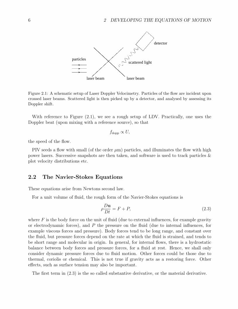
Figure 2.1: A schematic setup of Laser Doppler Velocimetry. Particles of the flow are incident uponcrossed laser beams. Scattered light is then picked up by a detector, and analysed by assessing itsDoppler shift.

With reference to Figure (2.1), we see a rough setup of LDV. Practically, one uses theDoppler beat (upon mixing with a reference source), so that

fdopp ∝ U,

the speed of the flow.

PIV seeds a flow with small (of the order µm) particles, and illuminates the flow with highpower lasers. Successive snapshots are then taken, and software is used to track particles &plot velocity distributions etc.

2.2 The Navier-Stokes Equations

These equations arise from Newtons second law.

For a unit volume of fluid, the rough form of the Navier-Stokes equations is

ρDu

Dt= F + P, (2.3)

where F is the body force on the unit of fluid (due to external influences, for example gravityor electrodynamic forces), and P the pressure on the fluid (due to internal influences, forexample viscous forces and pressure). Body forces tend to be long range, and constant overthe fluid, but pressure forces depend on the rate at which the fluid is strained, and tends tobe short range and molecular in origin. In general, for internal flows, there is a hydrostaticbalance between body forces and pressure forces, for a fluid at rest. Hence, we shall onlyconsider dynamic pressure forces due to fluid motion. Other forces could be those due tothermal, coriolis or chemical. This is not true if gravity acts as a restoring force. Othereffects, such as surface tension may also be important.

The first term in (2.3) is the so called substantive derivative, or the material derivative.

2.2 The Navier-Stokes Equations 7

2.2.1 The Material Derivative

We define an operator

D

Dt≡ ∂

∂t+ u · ∇ (2.4)

to be the material derivative. So, for example,

Du

Dt=∂u

∂t+ u · ∇u, (2.5)

which has the three components

Du

Dt= x

(∂u

∂t+ u

∂u

∂x+ v

∂u

∂y+ w

∂u

∂z

)+y

(∂v

∂t+ u

∂v

∂x+ v

∂v

∂y+ w

∂v

∂z

)+z

(∂w

∂t+ u

∂w

∂x+ v

∂u

∂y+ w

∂w

∂z

).

In index notation, (2.5) readsDuiDt

=∂ui∂t

+ uj∂ui∂xj

.

To understand the material derivative a bit better, or to get an intuition as to its meaning,one could consider a flow with

u = (u, v, w) = Ω(−y, x, 0),

which corresponds to a uniform rotation. Then,

u · ∇u = x(−Ω2x) + y(−Ω2y) = −Ω2(x, y),

which is a centrifugal acceleration Ω2r towards the centre of a circle.

The material derivative reflects the fact that fluid particles move from one location toanother in the flow, and can be accelerated/decellerated by both movement to a place ofhigher velocity as well as a temporal change in the global flow field. That is, fluid can beaccelerated in a steady flow.

One can think of the ∂∂t

term as a global derivative, and u · ∇ as a convective derivative.

For example, one could consider an aerofoil in uniform flow. The fluid flows faster over thetop than the bottom, which causes a change in pressure between the top and bottom, whichcauses lift.


2.2.2 Developing the Navier-Stokes Equations

We shall consider incompressible, viscous fluids, with pressure forces and the continuityequation.

Viscous Forces Consider a “box of fluid” ABCD, which is in a flow. Suppose that theheight of the box is δy. Then, the viscous forces acting in the top section of the box, in thex-direction, per unit area, is

µ

(∂u

∂y

)y+δy

δxδz.

Hence, the net viscous forces on a box is[µ

(∂u

∂y

)y+δy

−(∂u

∂y

)y

]δxδz.

If we let δy → 0, then this goes to a partial derivative, and so

∂

∂y

(µ∂u

∂y

)δxδyδz.

Hence, the net viscous forces, per unit volume, on a fluid element in the x-direction, is

µ∂2u

∂y2.

In a similar way, one can find the total viscous forces, in the x-direction, to be

µ

(∂2u

∂x2+∂2u

∂y2+∂2u

∂z2

)= µ∇2u. (2.6)

Hence, the viscous forces are given by

µ∇2u, (2.7)

which is linear in u. This is a diffusion term, where momentum is diffused into heat by theaction of viscosity – a kinematic force.

Pressure Forces The net pressure acting on an element in the downstream direction, isgiven by

(px − px+δx) δxδz.But,

px+δxδyδz =

(px +

∂p

∂x

)δyδz.

2.2 The Navier-Stokes Equations 9

Thus, the net pressure is

−∂p∂xδxδyδz,

or

−∂p∂x

per unit volume. Thus, in total, the net pressure forces, per unit volume, are given by

−∇p. (2.8)

Thus, notice that pressure acts in opposition to viscous forces.

Hence, the equations of motion are

∂u

∂t+ u · ∇u = −1

ρ∇p+ ν∇2u, (2.9)

where the molecular viscosity µ is related to the density ρ via the kinematic viscosity ν as

ν ≡ µ

ρ. (2.10)

Notice that using the material derivative and index notation, (2.9) reads

ρDuiDt

= − ∂p

∂xi+ µ

∂2ui∂x2

j

.

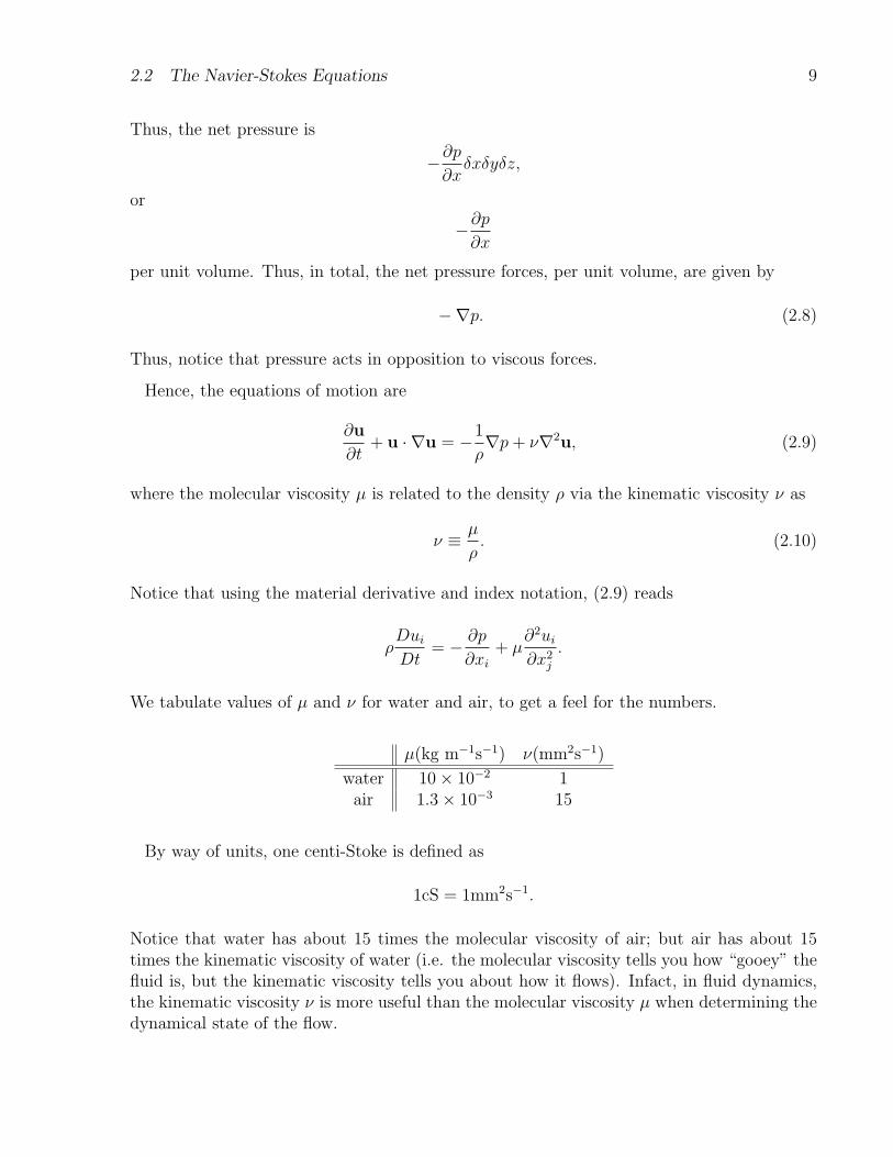
We tabulate values of µ and ν for water and air, to get a feel for the numbers.

µ(kg m−1s−1) ν(mm2s−1)

water 10× 10−2 1air 1.3× 10−3 15

By way of units, one centi-Stoke is defined as

1cS = 1mm2s−1.

Notice that water has about 15 times the molecular viscosity of air; but air has about 15times the kinematic viscosity of water (i.e. the molecular viscosity tells you how “gooey” thefluid is, but the kinematic viscosity tells you about how it flows). Infact, in fluid dynamics,the kinematic viscosity ν is more useful than the molecular viscosity µ when determining thedynamical state of the flow.


The Continuity Equation We have three equations (one for each component of (2.9))for four unknowns (the three velocity components, and density). Hence, we need a fourthequation. We appeal to a continuity equation.

Consider the rate of change of total mass outflux through some elemental surface,∫∂ρ

∂tdV = −

∫ρu · ndA.

Then, using the divergence theorem, this easily becomes∫ [∂ρ

∂t+∇ · (ρu)

]dV = 0.

Hence, as this is true for any volume, and indeed zero volume, the integrand must be zero.Therefore,

∂ρ

∂t+∇ · (ρu) = 0. (2.11)

If we expand out the divergence, we get

∂ρ

∂t+ ρ∇ · u + u · ∇ρ = 0,

where we note the material derivative of the density ρ is present in the first and third terms.Hence,

Dρ

Dt+ ρ∇ · u = 0. (2.12)

This is the continuity equation. For an incompressible fluid,

Dρ

Dt= 0 ⇒ ∇ · u = 0.

Navier-Stokes Equations Hence, we can write the Navier-Stokes equations, after ourrather wooly derivation. They are composed of the material derivative and continuity equa-tion. Thus:

∂u

∂t+ u · ∇u = −1

ρ∇p+ ν∇2u, (2.13)

∇ · u = 0. (2.14)

These are non-linear differential equations. The non-linearity comes from the second termfrom the left, on the first equation. There are three equations in the first, and a fourth in

2.3 Scaling Navier-Stokes & Reynolds Number 11

the second; hence, in full, the Navier-Stokes equations (in Cartesian coordinates) are

∂u

∂t+ u

∂u

∂x+ v

∂u

∂y+ w

∂u

∂z= −1

ρ

∂p

∂x+ ν

(∂2u

∂x2+∂2u

∂y2+∂2u

∂z2

),

∂v

∂t+ u

∂v

∂x+ v

∂v

∂y+ w

∂v

∂z= −1

ρ

∂p

∂y+ ν

(∂2v

∂x2+∂2v

∂y2+∂2v

∂z2

),

∂w

∂t+ u

∂w

∂x+ v

∂w

∂y+ w

∂w

∂z= −1

ρ

∂p

∂z+ ν

(∂2w

∂x2+∂2w

∂y2+∂2w

∂z2

),

∂u

∂x+∂v

∂y+∂w

∂z= 0.

We will mainly be concerned in deducing which terms go to zero, so that we can produce a“simple” analytic solution for a given situation. Non-linearity also enters in the boundaryconditions. The common boundary conditions are:

• Free stream far from boundaries:u = U0.

• Free stream at solid boundary:u · n = 0.

• No-slip:u× n = 0.

The last boundary condition, the no-slip condition, cannot be justified on a molecular level,but is very well supported by numerical and physical experiments. However, problems doarise in gas dynamics, where one has so-called “Knudsen layers of slip”.

2.3 Scaling Navier-Stokes & Reynolds Number

Consider a steady flow. Then, (2.13) reads

ρu · ∇u = −∇p+ µ∇2u. (2.15)

Now, we can introduce “new scales” for length and speed, so that

x∗ = x/L, y∗ = y/L, z∗ = z/L, u∗ = u/U0, ∆p∗ = ∆p/ρU20 .

The last quantity, ∆p is the difference between actual pressure, and some reference. Hence,all “starred” quantities are dimensionless. Hence, using these in (2.15) gives

U20

L(u∗ · ∇∗u∗) = −U

20

L∇∗ (∆p∗) +

νU0

L2(∇∗)2u∗,


or,

(u∗ · ∇∗u∗) = −∇∗ (∆p∗) +1

R∇∗2u∗,

where

R ≡ LU0

ν(2.16)

is the Reynolds number. This has the interpretation of telling you how big the inertia forcesare, relative to the viscous forces;

R =inertia

viscous.

Thus, if R > 1, the inertia forces dominate over viscous forces; and if R < 1, then viscousforces dominates inertia. Notice that it is the inertia term which has the non-linearity in theNS equations. Hence, one can see that if R 1, the NS equations become more linear,

−→ ∇p = µ∇2u.

If R→∞, then the equations become non-linear due to the inertia term u · ∇u:

−→ Du

Dt=

1

ρ∇p.

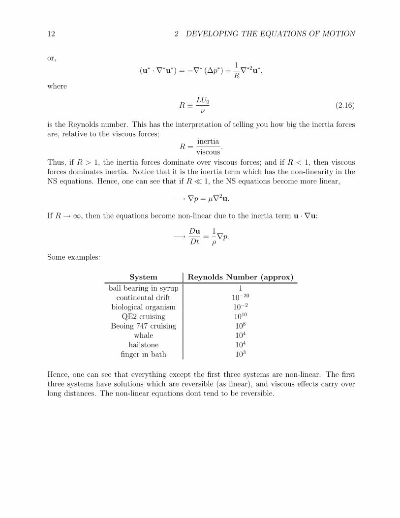
Some examples:

System Reynolds Number (approx)

ball bearing in syrup 1continental drift 10−20

biological organism 10−2

QE2 cruising 1010

Beoing 747 cruising 108

whale 104

hailstone 104

finger in bath 103

Hence, one can see that everything except the first three systems are non-linear. The firstthree systems have solutions which are reversible (as linear), and viscous effects carry overlong distances. The non-linear equations dont tend to be reversible.

13

3 Exact Solutions

Here we shall consider a few cases, and solve the Navier-Stokes equations exactly.

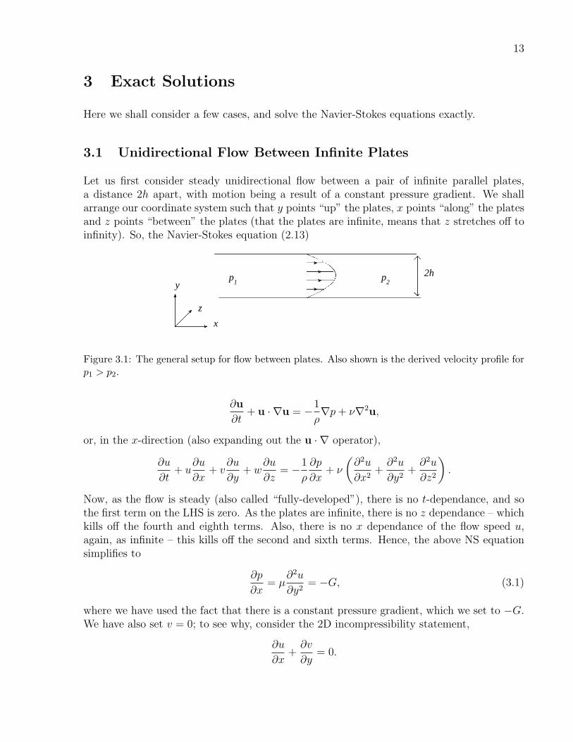
3.1 Unidirectional Flow Between Infinite Plates

Let us first consider steady unidirectional flow between a pair of infinite parallel plates,a distance 2h apart, with motion being a result of a constant pressure gradient. We shallarrange our coordinate system such that y points “up” the plates, x points “along” the platesand z points “between” the plates (that the plates are infinite, means that z stretches off toinfinity). So, the Navier-Stokes equation (2.13)

2h

x

z

yp

1p

2

Figure 3.1: The general setup for flow between plates. Also shown is the derived velocity profile forp1 > p2.

∂u

∂t+ u · ∇u = −1

ρ∇p+ ν∇2u,

or, in the x-direction (also expanding out the u · ∇ operator),

∂u

∂t+ u

∂u

∂x+ v

∂u

∂y+ w

∂u

∂z= −1

ρ

∂p

∂x+ ν

(∂2u

∂x2+∂2u

∂y2+∂2u

∂z2

).

Now, as the flow is steady (also called “fully-developed”), there is no t-dependance, and sothe first term on the LHS is zero. As the plates are infinite, there is no z dependance – whichkills off the fourth and eighth terms. Also, there is no x dependance of the flow speed u,again, as infinite – this kills off the second and sixth terms. Hence, the above NS equationsimplifies to

∂p

∂x= µ

∂2u

∂y2= −G, (3.1)

where we have used the fact that there is a constant pressure gradient, which we set to −G.We have also set v = 0; to see why, consider the 2D incompressibility statement,

∂u

∂x+∂v

∂y= 0.

14 3 EXACT SOLUTIONS

Now, suppose we introduce scales,

u ∼ U, v ∼ V, x ∼ L, y ∼ h.

Then, the “scaled” incompressibility equation reads

U

L+V

h= 0 ⇒ V ∼ Uh

L.

The last expression follows as we require both terms in the first expression to balance inorders. Now, as L h in our setup (infact, basically in everything we do), we have thatV ∼ 0. Therefore, we say that by dimensional scaling arguments, we set v = 0.

We can integrate (3.1), to see that

u(y) = A+By − Gy2

2µ, (3.2)

where A and B are constants of integration. Now, to go further, we need boundary conditions,so that we can determine A and B. Let us impose that the flow is stationary at the boundaries(i.e. the no-slip boundary condition). This corresponds to

u = 0 at y = ±h.So,

u(h) = A+Bh− Gh2

2µ= 0 ⇒ A = −Bh+

Gh2

2µ,

u(−h) = A−Bh− Gh2

2µ= 0 ⇒ A = Bh+

Gh2

2µ,

which is only satisfied byB = 0,

in which case

A =Gh2

2µ.

Hence, using these constants in the solution (3.2), we see that

u(y) =G

2µ

(h2 − y2

).

Thus, the velocity profile is parabolic, as in Figure (3.1). One can easily show that

umax =Gh2

2µ,

which is the speed in the middle of the plates. Now, this solution becomes unstable atR = 5772; that is, below this Reynolds number, experiment confirms this prediction verywell, but, above, non-linearity sets in and turbulence is observed.

3.2 Hagen-Poiseuille Flow 15

3.2 Hagen-Poiseuille Flow

Now consider fully developed steady flow in a long circular pipe, with a constant pressuregradient along the pipe.

We setup the cylindrical polar coordinate system; so that r is the distance from the centre,z the distance down, and θ an angle around the pipe.

We assume that the flow is of the form

u = (0, 0, uz(r)) ,

only. Also, by the definition of the problem,

∂p

∂r=∂p

∂θ= 0.

Recall the expressions for the grad, divergence and Laplacian, in cylindrical polar coordinates,

∇ =

(∂

∂r,1

r

∂

∂θ,∂

∂z

),

∇ · a =1

r

∂

∂r(rar) +

1

r

∂aθ∂θ

+∂az∂z

=arr

+∂ar∂r

+1

r

∂aθ∂θ

+∂az∂z

,

∇2a =1

r

∂

∂r

(r∂a

∂r

)+

1

r2

∂2a

∂θ2+∂2a

∂z2

=∂2a

∂r2+

1

r

∂a

∂r+

1

r2

∂2a

∂θ2+∂2a

∂z2.

Now, as we only have a uz component, the Navier-Stokes equation (for z) becomes

ρ

(∂uz∂t

+ ur∂uz∂r

+uθr

∂uz∂θ

+ uz∂uz∂z

)= −∂p

∂z+ µ

(∂2uz∂r2

+1

r

∂uz∂r

+1

r2

∂2uz∂θ2

+∂2uz∂z2

).

We can now simplify this, by noting that there is no time dependance, and u = (0, 0, uz(r))only, so that

0 = −∂p∂z

+ µ

(∂2uz∂r2

+1

r

∂uz∂r

),

also noting the constant pressure gradient

∂p

∂z= −G,

hence, the NS equation becomes

−Grµ

=d

dr

(rduzdr

).


We can now integrate this once,

−Gr2

2µ= r

duzdr

+ A,

but, if we divide through by r, then we see that

A

r− Gr

2µ=duzdr

.

Now, at r = 0, we have a singularity. Therefore, to get around this problem, we set A = 0.Hence,

−Gr2µ

=duzdr

,

which is integrated to give

uz(r) = −Gr2

4µ+B.

We then impose the boundary condition that uz(r = a) = 0 (where a is the radius of thepipe), so that

B =Ga2

4µ,

and hence the solution

uz =G

4µ(a2 − r2).

This is a parabolic velocity profile again.

Now, volume flow rate is computed via

Q =

∫ a

0

uz2πr dr =πGa4

8µ. (3.3)

If we take the pressure gradient to be

G =p0 − p1

l,

where l is the length of some pipe, and pi are the pressures at either end, then we see thatvolume flow rate is

Q ∝ p0 − p1

l, Q ∝ a4. (3.4)

These dependancies define Poiseuille’s law. Such an expression as (3.3) allows computationof the viscosity µ of a fluid, as flow rate Q and radius a are relatively simple to measure.

Now, Poiseuille’s law is only accurate for R < 30 (for all pipes). For greater Reynoldsnumber R, the pipe must be “long enough” to establish an x-independent solution, otherwisethe entrance of the fluid into the pipe effects the results. The general rule is

x

d=R

30, (3.5)

3.3 Flow Down Inclined Plane 17

so that for a flow with Reynolds number R, through a pipe of diameter d, then the lengthof the pipe needs to be x in order that Poiseuille’s law holds. For example, if R = 1800, oneneeds 60 diameters length of a pipe such that Poiseuille’s law can be applied.

Notice that as the Poiseuille effect has been experimentally verified, then the no-slip bound-ary condition is valid, as it was used in the derivation.

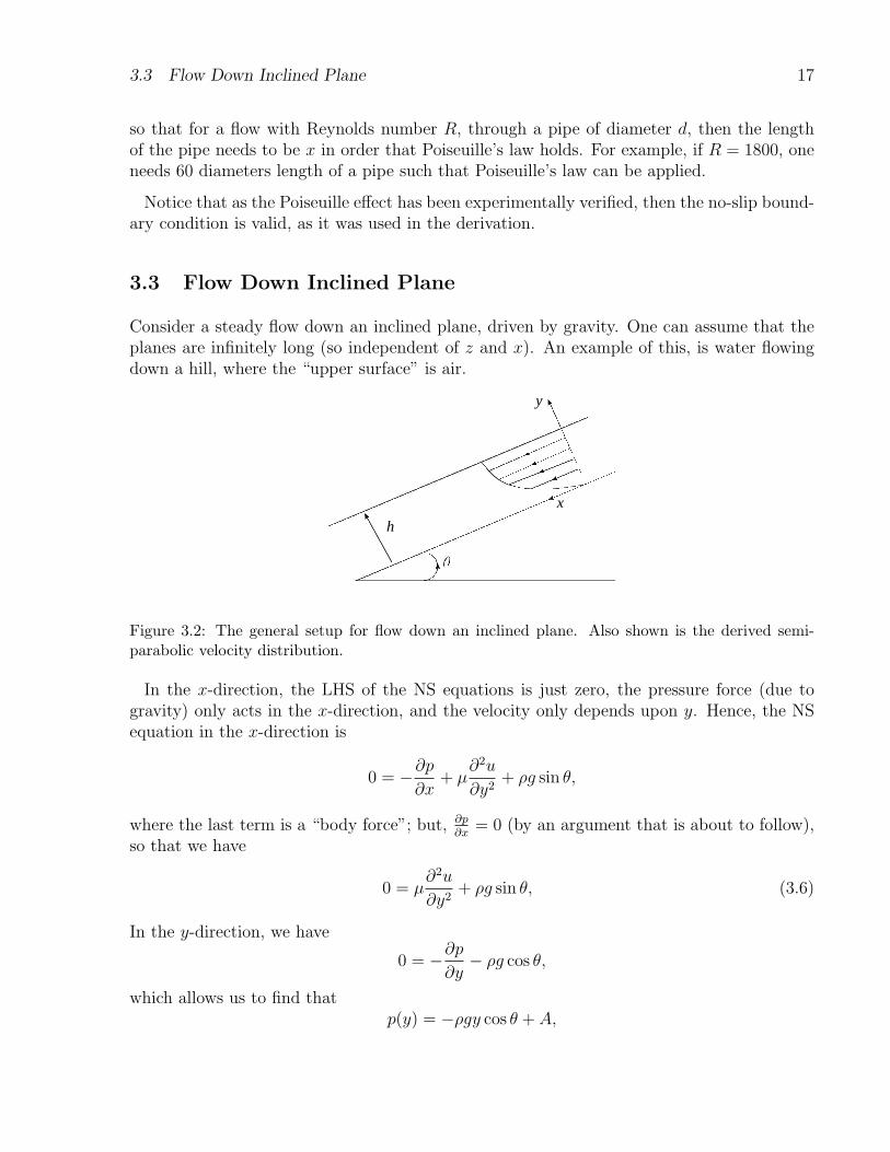
3.3 Flow Down Inclined Plane

Consider a steady flow down an inclined plane, driven by gravity. One can assume that theplanes are infinitely long (so independent of z and x). An example of this, is water flowingdown a hill, where the “upper surface” is air.

h

y

x

Figure 3.2: The general setup for flow down an inclined plane. Also shown is the derived semi-parabolic velocity distribution.

In the x-direction, the LHS of the NS equations is just zero, the pressure force (due togravity) only acts in the x-direction, and the velocity only depends upon y. Hence, the NSequation in the x-direction is

0 = −∂p∂x

+ µ∂2u

∂y2+ ρg sin θ,

where the last term is a “body force”; but, ∂p∂x

= 0 (by an argument that is about to follow),so that we have

0 = µ∂2u

∂y2+ ρg sin θ, (3.6)

In the y-direction, we have

0 = −∂p∂y− ρg cos θ,

which allows us to find thatp(y) = −ρgy cos θ + A,


but, at y = h, p = p0, the atmospheric pressure. Hence

p− p0 = ρg(h− y) cos θ,

which is the reason we said that ∂p∂x

= 0. The boundary conditions we use are no slip on thesurface. Thus, u = 0 at y = 0. Also, there is to be no shear stress, in which case

τxy = µ

(∂u

∂y− ∂v

∂y

)= 0,

but the first term is zero, so∂u

∂y= 0

at y = h. From (3.6),

µ∂2u

∂y2= −ρg sin θ,

and so integrating gives

µ∂u

∂y= −ρgy sin θ + A,

but, by the free surface boundary condition, the LHS is zero at y = h, so that

A = ρgh sin θ.

Hence,∂u

∂y=g sin θ

ν(h− y),

integrating again,

u(y) =g sin θ

ν

(hy − 1

2y2

)+B,

but, using u(y = 0) = 0, one sees that B = 0. Hence, the velocity profile is

u(y) =g sin θ

ν

(hy − 1

2y2

).

This profile is a semi-parabola, as in Figure (3.2).

Now, the average velocity flow over the layer is

u =1

h

∫ h

0

u dy =1

3

g sin θ

νh2.

Notice that the surface speed, u(y = h) is

usurface = u(h) =1

2

g sin θ

νh2,

3.4 Unsteady Flow 19

and hence that

u(h) =3

2u.

Again, all of the above is for R < 20. Otherwise, non-linear effects come into play – suchas “roll waves” on the surface. Considering rain flowing down a road. A typical speed isu = 10cms−1, with depth d = 2mm and kinematic viscosity ν = 1cS. This gives R = 200,and so one would expect (and indeed sees) to see roll waves.

3.4 Unsteady Flow

Let us consider a time dependent flow. Let a viscous fluid fill the half plane above a boundary,and let the boundary move in a tangential direction, periodically; as in Figure (3.3).

u=u0

x

y

Figure 3.3: The general setup for an unsteady flow. A fluid fills the plane above some boundary,where the boundary moves periodically such that u = u0 cosωt.

We shall assume that everything is uniform, in the x-direction, and no z-dependance (sov = w = 0). Hence, the NS equation, in the x-direction, is just

∂u

∂t= ν

∂2u

∂x2, (3.7)

We use the boundary condition that as y → ∞, u → 0. Also, we have that at y = 0,u(y = 0) = u0 cosωt = <(u0e

iωt). Hence, we shall seek a solution of the form

u(y, t) = f(y)eiωt.

So, using this, (3.7) becomes

iω

νf =

d2f

dy2. (3.8)


If we denote

α2 ≡ iω

ν,

then the solution to (3.8) isf(y) = Aeαy +Be−αy.

Now, our requirement is that the velocity should not diverge as y → ∞; hence, we requirethat A = 0. Also, at y = 0, we require f(y = 0) = u0 by the boundary condition. Hence,

f(y) = u0e( iων )

1/2y,

and therefore,

u(y, t) = u0e( iων )

1/2yeiωt. (3.9)

Now, if we use the identity that √i =

1 + i√2,

and the definition that

k ≡√

ω

2ν,

then we see that (3.9) can be written as

u(y, t) = u0e−(1+i)kyeiωt = u0e

−kyei(ωt−ky),

which is a damped travelling wave, propagating in the y-direction. Recall that we must takethe real part of this expression, so that

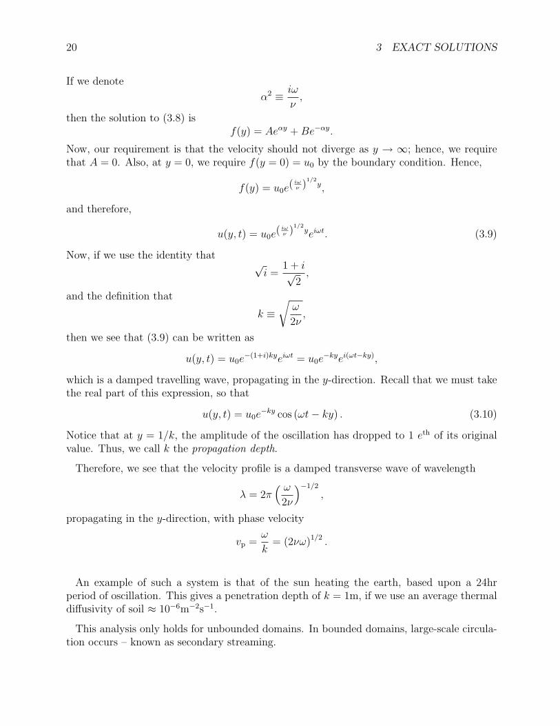
u(y, t) = u0e−ky cos (ωt− ky) . (3.10)

Notice that at y = 1/k, the amplitude of the oscillation has dropped to 1 eth of its originalvalue. Thus, we call k the propagation depth.

Therefore, we see that the velocity profile is a damped transverse wave of wavelength

λ = 2π( ω

2ν

)−1/2

,

propagating in the y-direction, with phase velocity

vp =ω

k= (2νω)1/2 .

An example of such a system is that of the sun heating the earth, based upon a 24hrperiod of oscillation. This gives a penetration depth of k = 1m, if we use an average thermaldiffusivity of soil ≈ 10−6m−2s−1.

This analysis only holds for unbounded domains. In bounded domains, large-scale circula-tion occurs – known as secondary streaming.

3.5 Steady Driven Flow With Inflow 21

Figure 3.4: The derived solution (3.10) for unsteady flow. The boundary is on the LHS, with wavepropagating from left to right.

3.5 Steady Driven Flow With Inflow

Consider viscous flow between rigid planes at y = 0, h, where the lower plane moves atconstant speed u0 in the x-direction, and the walls (i.e. the planes) are porous, allowing (andindeed, we enforce) a constant vertical flow v0. See Figure (3.5).

y = 0

y = h

u(y)

u0v

0

v0

x

y

Figure 3.5: The general setup for flow between two porous planes.

We make the plates infinite in extent into the z-direction, so that

u = (u(y), v(y), 0)

only. Notice that we do not have any x-dependance upon the velocity; this is because we areconsidering fully developed flow.


Notice that we can write the incompressibility law,

∇ · u =∂u

∂x+∂v

∂y=∂v

∂y= 0,

where the second equality follows as u is not a function of x, and only of y. Hence, integrating,we see that v = const, and we set v = −v0 (with a minus sign as the direction of flow is“down”, opposite to the direction of +y).

The steady Navier-Stokes equations are

u · ∇u = −1

ρ∇p+ ν∇2u,

so that writing out its two components, we have

u∂u

∂x+ v

∂u

∂y= −1

ρ

∂p

∂x+ ν

∂2u

∂x2+ ν

∂2u

∂y2, (3.11)

u∂v

∂x+ v

∂v

∂y= −1

ρ

∂p

∂y+ ν

∂2v

∂x2+ ν

∂2v

∂y2. (3.12)

The first and fourth terms of the first expression are zero (as no x-dependance of u). Also,the first, second, fourth and fifth terms of the second expression are zero (as no x-dependanceof v and v is a constant). So, (3.11) becomes

− v0∂u

∂y= −1

ρ

∂p

∂x+ ν

∂2u

∂y2. (3.13)

And we see that (3.12) becomes

0 = −1

ρ

∂p

∂y⇒ p = p(x).

If we impose that p = p0 at x = ±∞, then we also have that p = const, so that motion isdriven purely by the fluid flow, and not by a pressure gradient. Hence, (3.13) becomes

ν∂2u

∂y2+ v0

∂u

∂y= 0.

This has the easily verifiable solution,

u(y) = A+Be−v0yν .

If we now impose boundary conditions, we can find the values of the constants A,B. Wehave the no-slip boundary condition that u = 0 on y = h, which gives us

A = −Be− v0hν ⇒ u(y) = B(e−

v0yν − e− v0hν

).

3.5 Steady Driven Flow With Inflow 23

We also have that u = u0 on y = 0. Hence,

u0 = B(

1− e− v0hν)⇒ B =

u0

1− e− v0hν,

and therefore, the velocity profile is given by

u(y) = u0e−

v0yν − e− v0hν

1− e− v0hν. (3.14)

See Figure (3.6) for plots of the solution, in the cases of v0 small and large – (a) and (b),respectively.

0.0 0.2 0.4 0.6 0.8 1.0uHyL0.0

0.2

0.4

0.6

0.8

1.0y

(a) v0 small.

0.0 0.2 0.4 0.6 0.8 1.0uHyL0.0

0.2

0.4

0.6

0.8

1.0y

(b) v0 large.

Figure 3.6: Two limiting cases of the solution (3.14) to the steady driven flow with porous bound-aries; in these plots, the moving boundary is along the x-axis. We see in (a) that the velocity profileapproaches linear, when the speed of the inflow is very small. In (b) we see that the profile shiftsmost of the motion towards the moving wall, an example of a boundary layer.

Consider taking v0h/ν 1 in (3.14), expanding the exponentials,

u(y) ≈ u0

1− v0yν− (1− v0h

ν

)1− (1− v0h

ν

) = u0

(1− y

h

),

which is a linear profile, as in Figure (3.6)a. This is a linear shear flow, also called Couretteflow. The other limit we can take, in (3.14) is v0 large, in which case

u(y) ≈ u0e− v0y

ν ,

which effectively confines the flow to the lower (moving) wall. That is, u is very small, exceptat the moving boundary. This is an example of a boundary layer. This boundary layer is nota typical one (more on this later), but one can see that its thickness is ≈ ν.


3.6 Low Reynolds Number Flow: Stokes Flow

Recall that the Navier-Stokes equations for steady flow of an incompressible fluid are

∇ · u = 0, u · ∇u = −1

ρ∇p+ ν∇2u.

Now, the ratio of the viscous and inertia terms are such that

1

R=

viscous

inertia.

Therefore, if R 1, the viscous terms dominate, and we can ignore the inertia terms. Suchflow is called creeping flow, and one has the Stokes equations,

∇ · u = 0, ∇p = µ∇2u. (3.15)

Recall that the ∇2u-term is a viscous term, and so the second equation of the above is abalance between dynamical pressure and viscous forces.

We could also use another argument of scale out inertia terms; for example, in thin-filmflows, where viscosity acts over small length scales, such as in lubrication layers. Hence, withthe usual scalings, u ·∇u ∼ u2/d and ν∇2u ∼ νu/h2, the creeping flow requirement becomes

R 1 ⇒ u2

d νu

h2.

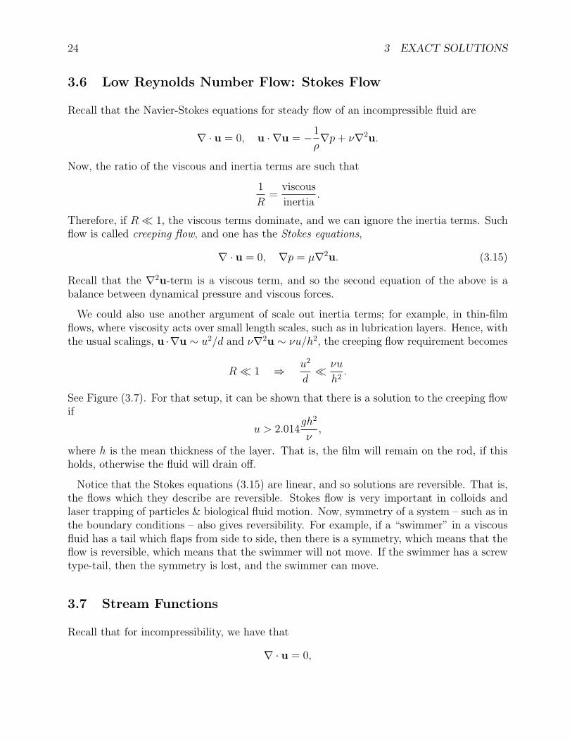
See Figure (3.7). For that setup, it can be shown that there is a solution to the creeping flowif

u > 2.014gh2

ν,

where h is the mean thickness of the layer. That is, the film will remain on the rod, if thisholds, otherwise the fluid will drain off.

Notice that the Stokes equations (3.15) are linear, and so solutions are reversible. That is,the flows which they describe are reversible. Stokes flow is very important in colloids andlaser trapping of particles & biological fluid motion. Now, symmetry of a system – such as inthe boundary conditions – also gives reversibility. For example, if a “swimmer” in a viscousfluid has a tail which flaps from side to side, then there is a symmetry, which means that theflow is reversible, which means that the swimmer will not move. If the swimmer has a screwtype-tail, then the symmetry is lost, and the swimmer can move.

3.7 Stream Functions

Recall that for incompressibility, we have that

∇ · u = 0,

3.7 Stream Functions 25

d u

h

g

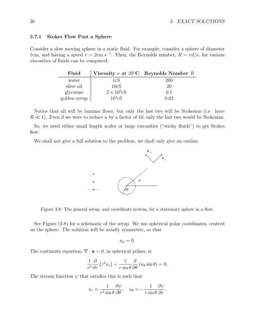
Figure 3.7: An example of a thin viscous layer between two surfaces; it can be shown that there isa solution to the creeping equations of motion.

or, for a 2D flow,∂u

∂x+∂v

∂y= 0.

Suppose we introduce some function ψ, such that

u =∂ψ

∂y, v = −∂ψ

∂x,

then we see that the divergence of u is still zero. Thus, we have replaced two functions, u, vby a single stream function ψ.

Notice that

dψ =∂ψ

∂xdx+

∂ψ

∂ydy

= −vdx+ udy. (3.16)

Now, on a streamline,dx

u=dy

v⇒ v = u

dy

dx,

hence, using this in (3.16), we see that

dψ = −udy + udy = 0.

That is, dψ is zero on a streamline. This is equivalent to saying

ψ = const on a streamline.

Also, one could say that streamlines are lines of constant ψ. Streamlines cannot cross, exceptat stagnation points.


3.7.1 Stokes Flow Past a Sphere

Consider a slow moving sphere in a static fluid. For example, consider a sphere of diameter1cm, and having a speed v = 2cm s−1. Then, the Reynolds number, R = vd/ν, for variousviscosities of fluids can be computed:

Fluid Viscosity ν at 20C Reynolds Number R

water 1cS 200olive oil 10cS 20glycerine 2× 103cS 0.1

golden syrup 104cS 0.02

Notice that all will be laminar flows, but only the last two will be Stokesian (i.e. haveR 1). Even if we were to reduce u by a factor of 10, only the last two would be Stokesian.

So, we need either small length scales or large viscosities (“sticky fluids”) to get Stokesflow.

We shall not give a full solution to the problem, we shall only give an outline.

ur

u

a

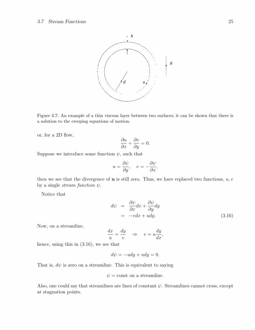
Figure 3.8: The general setup, and coordinate system, for a stationary sphere in a flow.

See Figure (3.8) for a schematic of the setup. We use spherical polar coordinates, centredon the sphere. The solution will be axially symmetric, so that

uφ = 0.

The continuity equation, ∇ · u = 0, in spherical polars, is

1

r2

∂

∂r

(r2ur

)+

1

r sin θ

∂

∂θ(uθ sin θ) = 0.

The stream function ψ that satisfies this is such that

ur =1

r2 sin θ

∂ψ

∂θ, uθ = − 1

r sin θ

∂ψ

∂r.

3.7 Stream Functions 27

In Stokes’ equations, we have a term ∇2u. We will use the vector identity

∇2u = ∇(∇ · u)−∇×∇× u = −∇×∇× u,

to clean the expression up. The second equality follows due to the incompressibility of thefluid. Hence, in spherical polars, the Stokes equations read

∂p

∂r=

µ

r2 sin θ

∂

∂θ

[∂2ψ

∂r2+

sin θ

r2

∂

∂θ

(1

sin θ

∂ψ

∂θ

)],

1

r

∂p

∂θ= − µ

r sin θ

∂

∂r

[∂2ψ

∂r2+

sin θ

r2

∂

∂θ

(1

sin θ

∂ψ

∂θ

)].

We can eliminate p to find [∂2

∂r2+

sin θ

r2

∂

∂θ

(1

sin θ

∂

∂θ

)]2

ψ = 0.

This homogeneous differential equation can be solved via standard techniques, such as apower series solution, subject to appropriate boundary conditions. The boundary conditionswe use are

ur(r →∞) = u0 cos θ, uθ(r →∞) = −u0 sin θ,

ur(r = a) = 0, uθ(r = a) = 0.

The first line of conditions impose a free streaming flow from infinity, with free-streamingspeed u0, and the second set impose no-slip (that is, no flow across material surface). Thesolution to the differential equation is then given by

ur = u0 cos θ

(1− 3a

2r+

a3

2r3

),

uθ = −u0 sin θ

(1− 3a

4r2− a3

2r3

),

p− p0 = −3µu0a

2r2cos θ;

where p0 is the hydrostatic pressure. We can use these solutions to compute the streamfunc-tion,

ψ =u0r

2

sin2 θ

(3a

4r− a3

4r3

).

Notice that the “lead term” is 1/r, rather than 1/r2, which means that the influence of theflow can travel very far, meaning that boundaries can have a large effect in experiment.

So, we have computed the solution to a low Reynolds number flow past a sphere.

Notice that the solution is symmetric – this is a reflection of the linearity of the problem.


A B

Figure 3.9: The streamlines in a Stokes flow past a sphere.

Let us then consider the point force at the surface of the sphere. The shear force is

σ = −µ(∂uθ∂r

)r=a

sin θ − (p− p0)r=a cos θ

=3µu0

2a.

Notice that this is independent of θ. Hence, the total force D, is just σ multiplied by thesurface area of the sphere,

D = 4πa2σ = 6πµau0.

Now, consider the balance between this total force, and a bouyancy force,

6πµau0 =4

3πa3 (ρ− ρ) g,

where ρ is the density of the fluid, and ρ the density of the sphere – this is only true forR 1. Then, one can easily use this to write the Reynolds number,

R =2au

ν=

4a3g

9ν2

(ρ

ρ− 1

) 1.

Consider a sand grain falling in water. Then, ρ/ρ ∼ 2 and ν = 1cS (at T = 20C), hence,the Reynolds number must be smaller than R = 4.4 × 104a3. That is, for a Stokesianflow, a < 0.03mm. Further consider a (solid) raindrop, with ρ/ρ ∼ 780, ν = 15cS, thena < 0.04mm. Finally consider a steel ball in syrup: ρ/ρ ∼ 7, ν = 1.2 × 104cS givinga < 1.65mm.

We define the viscous drag coefficient

CD =2D

ρu2a2=

6π

R. (3.17)

The symbol CD is used as a general viscous drag coefficient, but here we have written anexpression only for Stokesian flows; either way, CD is unimportant for R > 1.

Now consider the case of a non-rigid sphere – an inviscid drop in an immiscible viscousfluid. For example, a water-oil interface. The normal components of the velocity are equal,and there is no relative motion of the fluids at the interface; tangential stress is continuous

3.8 Steady Inviscid Flows 29

across the interface – equal and opposite across the interface. All other conditions are as inthe solid sphere case. The solution is

u =a2g

3ν

(ρ

ρ− 1

)µ+ µ

µ+ 32µ.

We have that µ/µ = 0 corresponds to a solid, which gives the Stokes result; and µ/µ = 0for a viscous liquid. This result can be used in experiment to test the purity of a liquid. Ifa liquid has impurities – dirt – then, the impurities accumulate at the interface, giving anessentially solid shell, thus changing the speed.

3.8 Steady Inviscid Flows

Let us now consider flows which have ν → 0, so that R→∞. This also works for flows withlarge u0.

The steady Navier-Stokes equations are

u · ∇u = −1

ρ∇p+ ν∇2u, ∇ · u = 0;

or, if we appropriately scale them, we have

u∗ · ∇∗u∗ = −1

ρ∇∗p∗ +

1

R(∇∗)2u∗.

Then, letting R→∞, we see that this just becomes (leaving off the stars),

u · ∇u = −1

ρ∇p. (3.18)

This is known as Euler’s equation. This is now a first order differential equation, which meansthat we require less boundary conditions. We tend to retain the impermeability boundarycondition, but reject the no-slip condition. This gives something of a paradoxical situation;as the Reynolds number R increases, the Euler solutions are found to become better andbetter approximations, however, in practice, viscosity is still effective at boundaries, so thatno-slip holds, but we can choose to ignore no-slip in solving Euler’s equations. The resolutionof this comes when we make a better choice of length scales, giving boundary layers.

Let us consider a streamline in an inviscid flow, governed by Euler’s equation. Suppose wedenote the distance along the streamline by `. At any point on the streamline, the componentof Euler’s equation along the streamline is just

ρq∂q

∂`= −∂p

∂`,

where q is some speed. Integrating this easily gives us that

1

2ρq2 + p = const on a streamline. (3.19)


This is Bernoulli’s equation. One can think of the first term as a “kinetic energy”. Hence, ifwe have high pressure, then we must have low speed; and vice-versa.

We could extend Bernoulli’s equation, by considering the vector identity

u · ∇u =1

2∇u2 − u×∇× u

in the LHS of (3.18). Using the definition of vorticity,

ω ≡ ∇× u,

but imposing irrotational flow (more on this later), then we see that

u · ∇u =1

2∇q2.

Therefore, using this in Euler’s equation (3.18), we see that

∇(

1

2ρq2 + p

)= 0,

which only holds for irrotational flow.

Therefore, we have seen that 12ρq2 + p is a constant throughout the flow, using Bernoulli,

where the constant is the same per streamline.

Figure 3.10: Circular streamlines in a uniform flow. The constant of Bernoulli is the same along agiven streamline.

3.8.1 D’Alembert’s Paradox

A consequence of the inviscid flow model, is the lack of drag for a symmetric object placedin a flow.

Consider a cylinder placed in a flow, as in Figure (3.9). Consider the streamline that hitsthe middle of the cylinder (such as at point A), and that it travels around and leaves thecylinder at B. Then, by Bernoulli,

pA = pB =1

2ρu2

0 + p0.


That is, the pressure difference is the same along the streamline, which means that there isno net pressure difference, which means that there is no drag. Therefore, upon placing sucha cylinder in such a flow, one would not see the cylinder get carried along by the flow. Thispressure distribution is the same as for the undisturbed flow (i.e. flow with no cylinder).

Infact, it can be shown that there will be zero drag for non-symmetric obstacles.

3.8.2 Applications of Bernoulli’s Theorem

hA

hB

hC

SB

SA

Figure 3.11: The Venturi tube for measuring flow rates. The cross-sectional areas are denoted SA

and SB.

The Venturi Tube Consider the setup in Figure (3.11). We have a flow of density ρcoming in from the right, through a tube of cross-sectional area SA, the flow is forced intoa smaller tube of cross-section SB, and comes out again the other side. At each tube is amanometer tube, which allows the height of the fluid to be read off.

Notice that streamlines are closer together in the middle tube, than in the LHS tube – thismeans that the flow is faster in the middle than the LHS tube. The cross-sectional area ofthe RHS tube is the same as the LHS tube, so, one would naively assume that hA = hC –this is not true, as vortices tend to be created when the fluid leaves the smaller tube, thusleaving hC < hA. The Venturi tube is used to measure fluid flow rates, as one can computethe flow rate given hA and hB, as we shall now show.

Consider applying Bernoulli’s equation (3.19) to the central streamline. Then,

1

2u2

A +pA

ρ=

1

2u2

B +pB

ρ,

⇒ u2A − u2

B =2

ρ(pB − pA) .

Now, the pressure difference is just

pA − pB = ρg (hA − hB) ,


and hence

u2A − u2

B = −2g (hA − hB) . (3.20)

Now, the equation of continuity, for an incompressible fluid,

uASA = uBSB,

allows us to see that

uB =uASA

SB

,

and hence upon substitution into (3.20),

uA =

2g(hA − hB)S2

A

S2B− 1

1/2

.

Therefore, we have a way of measuring the input flow speed for a fluid entering a Venturitube.

hA

hB

A

B

Figure 3.12: Flow from a hole in a tank. The fluid height is hA, and the hole is at a height hB, andthe fluid leaves the hole with velocity u.

Flow from a Hole in a Tank Consider a setup as in Figure (3.12). Let us assume thatthe top level of the fluid drops slowly, so that we can neglect the velocity of the free surface.Hence, uA = 0. Thus, applying Bernoulli’s equation to the streamline shown in the diagram,

pA

ρ=pB

ρ+

1

2u2. (3.21)

The pressure difference is just

pA − pB = ρg (hA − hB) = ρgh,


where h ≡ hA − hB is the distance between the hole and the top of the fluid. Hence, usingthis in (3.21), we see that

1

2u2 = gh,

and hence the speed of the fluid when it leaves the hole

u =√

2gh.


35

4 Vorticity

Recall that we defined the curl of the velocity field to be vorticity,

ω ≡ ∇× u. (4.1)

Now, consider a 2D flow,u = (u(x, y, t), v(x, y, t), 0) ,

hence, one can easily see that vorticity has only one component,

ω = (0, 0, ω) , ω ≡ ∂v

∂x− ∂u

∂y.

Vorticity gives a local measure of spin of a fluid element – it does not tell you that the globalvelocity field is rotating.

Consider that

v(x+ δx, y, t)− v(x, y, t) =∂v

∂xδx, u(x, y + δy, t)− u(x, y, t) =

∂u

∂yδy;

which follows from the definition of partial derivatives. Hence, taking their difference, wehave

1

2ω =

1

2

(∂v

∂x− ∂u

∂y

).

Thus, vorticity is the average angular velocity of two short fluid elements.

Consider the vector identity,

∇× (u · ∇u) = u · ∇(∇× u)− (∇× u) · ∇u + (∇ · u)(∇× u).

The last term is zero by incompressibility, ∇ · u = 0, and we write the other terms in termsof ω, so that

∇× (u · ∇u) = u · ∇ω − ω · ∇u. (4.2)

Let us write the Navier-Stokes equation

∂u

∂t+ u · ∇u = −1

ρ∇p+ ν∇2u + F,

where F is some body force; take its curl,

∂ω

∂t+∇× u · ∇u = ν∇2ω +∇× F.

Now, as we can write F as the grad of a scalar, and the curl grad is zero, then the curl of Fis zero. Also, we write the second term on the LHS using (4.2),

∂ω

∂t+ u · ∇ω − ω · ∇u = ν∇2ω,

36 4 VORTICITY

we can then write the first two terms on the LHS in terms of the material derivative, so that

Dω

Dt− ω · ∇u = ν∇2ω. (4.3)

This is known as the vorticity equation.

We commonly will consider steady flows, so that

∂ω

∂t= 0.

What this means, is that if there is no initial vorticity, then there is never vorticity.

A flow is called irrotational if ω = 0.

4.1 Examples

Let us consider some examples.

4.1.1 Irrotational Flow

Consider a flow with

uθ =Ωa2

r, ur = uz = 0.

Then, vorticity is given by

ω = ∇θ × Ωa2

r=

1

r

∂

∂r

(r

Ωa2

r

)= 0.

Now, this is only defined for r 6= 0; so that we can only say that the flow is irrotationaloff-axis. To see this, consider Stokes’ theorem,∮

u · d` =

∫∇× u · dS =

∫ω · dS.

So, integrating at fixed r gives 2πΩa2. However, we showed that the flow was irrotational.Therefore, everywhere, except at r = 0, the flow is irrotational; and all vorticity is concen-trated at r = 0. See Figure (4.1)a.

4.1.2 Solid Body Rotation

Consider a fluid element as in Figure (4.1)b, where u = Ω× r, so that vorticity is given by

ω = ∇×Ω× r =

∣∣∣∣∣∣i j k∂∂x

∂∂y

∂∂z

−Ωy Ωx 0

∣∣∣∣∣∣ = 2Ωk.

4.1 Examples 37

(a) Irrotationalflow.

(b) Solid body ro-tation.

Figure 4.1: Irrotational flow – as the fluid moves round, it retains its alignment. Also shown is solidbody rotation.

Hence, we see that a change in the orientation of a fluid element gives rise to vorticity;where vorticity is twice the rotational velocity of the fluid element.

4.1.3 Hele-Shaw Flow

Consider the setup as in Figure (4.2). We are considering thin film flow, where two glassplates have a very narrow uniform gap h (of the order mm).

0

h

x

y

z

Figure 4.2: Hele-Shaw flow between two glass plates which are very close together.

We impose the no-slip boundary condition at z = 0, h. In the z-direction, viscosity domi-nates, so that the Navier-Stokes equations become

u = − 1

2µ

∂p

∂xz(h− z), v = − 1

2µ

∂p

∂yz(h− z).

Notice that this is quadratic in z. Also notice that each flow component u, v depend uponz, but, their ratio does not. Hence, the pressure p is a function of x, y only. If we cross-differentiate, and subtract, we arrive at the interesting result

∂v

∂x− ∂u

∂y= 0.

This is the expression for vorticity, and hence Hele-Shaw flow is equivalent to an irrotationalflow. Applications of such flow include flow through porous media – such as soils and oilbearing rock – which can be considered statistically uniform.

38 4 VORTICITY

4.2 Irrotational Flow & The Complex Potential

Irrotational flow is important in many practical situations, including flow far from boundariesand atmospheric flows.

Let us consider only 2D irrotational flows, so that

∇× u = 0 ⇒ ωz =∂v

∂x− ∂u

∂y= 0.

Now, we can replace the velocity vector by a velocity potential φ, so that

u = −∇φ.

Hence,

u = −∂φ∂x, v = −∂φ

∂y.

The incompressibility statement ∇ · u = 0 allows us to also write

u = −∂ψ∂y, v =

∂ψ

∂x;

where ψ is the streamfunction, as already discussed. Hence, equating these expressions, wehave

∂φ

∂x=∂ψ

∂y,

∂φ

∂y= −∂ψ

∂x. (4.4)

These equations are known as the Cauchy-Riemann equations, and are familiar from complexanalysis. Notice that both the streamfunction ψ and velocity potential φ are harmonicfunctions;

∇2φ = ∇2ψ = 0.

Also notice that

∇φ · ∇ψ =∂φ

∂x

∂ψ

∂x+∂φ

∂y

∂ψ

∂y= 0,

so that we can see that equipotential lines are orthogonal to streamlines – except at stagnationpoints, where velocity is zero.

If the partial derivative are zero, we can define the complex potential w,

w = φ+ iψ. (4.5)

Thus, we see that the complex potential is a function of a complex variable z = x + iy.Expressing flows in terms of the complex potential w makes analysis of flows much simpler.Let us consider some examples.

4.2 Irrotational Flow & The Complex Potential 39

4.2.1 Examples of w-flows

Consider a flow withw = z2.

Then,z2 = (x+ iy)(x+ iy) = x2 − y2 + 2ixy.

Therefore, as φ is the real part of w, and ψ the complex part,

φ = x2 − y2, ψ = 2xy.

x

y

C

BA

D

Figure 4.3: Flow round a corner, given by w = z2. Solid lines are streamlines, dashed lines are linesof equipotential.

See Figure (4.3) for a visualisation of the flow. Notice that the box ABCD retains its area,but as it moves from right to left, AB,DC are compressed, and AD,BC are stretched. Thebox changes shape, but keeps its sides parallel to the axes – hence, the flow is irrotational.

A second case we consider is a generalisation of w = z2;

w = Ua(za

)π/α, (4.6)

so that flow motion takes place contained by two boundaries with internal angle α, a is alength scale and U the speed of the flow.

With reference to Figure (4.4), we see various flow diagrams for various angles α.

Also, consider a flow with complex potential

w =Uz2

a. (4.7)

Hence, streamlines are given by ψ = 2Uaxy

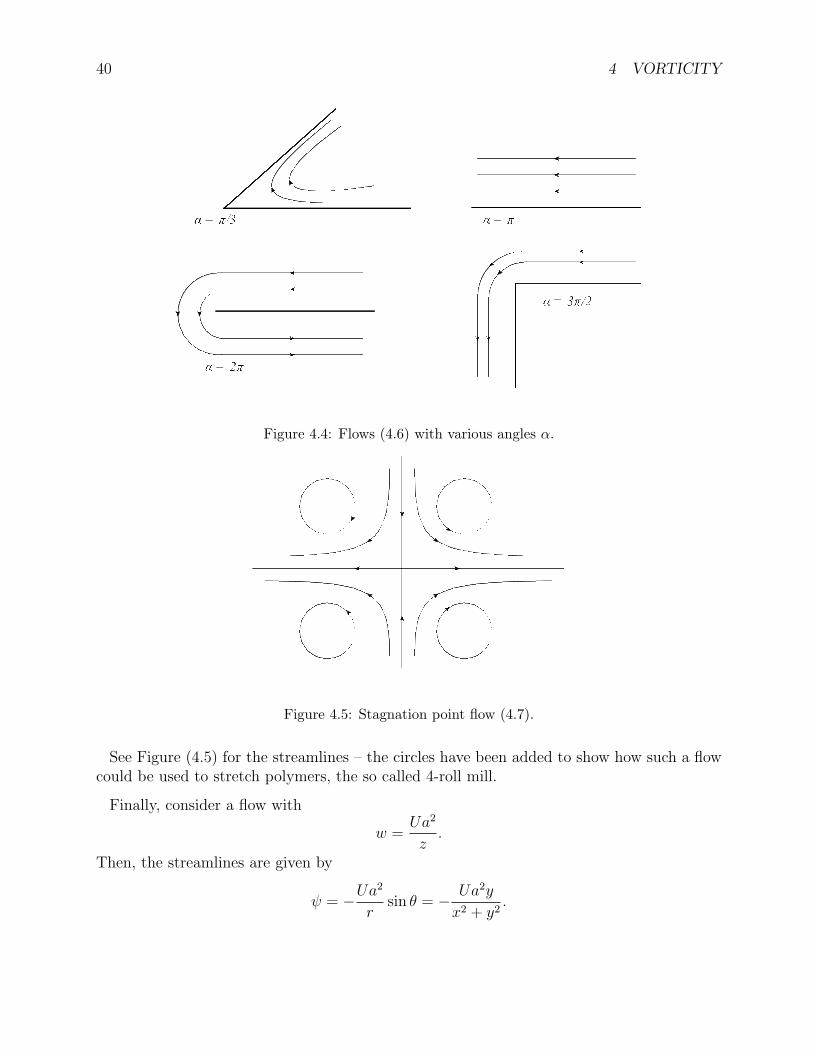
40 4 VORTICITY

Figure 4.4: Flows (4.6) with various angles α.

Figure 4.5: Stagnation point flow (4.7).

See Figure (4.5) for the streamlines – the circles have been added to show how such a flowcould be used to stretch polymers, the so called 4-roll mill.

Finally, consider a flow with

w =Ua2

z.

Then, the streamlines are given by

ψ = −Ua2

rsin θ = − Ua2y

x2 + y2.

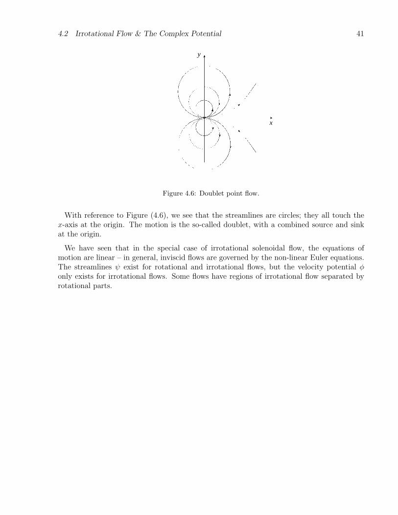
4.2 Irrotational Flow & The Complex Potential 41

x

y

Figure 4.6: Doublet point flow.

With reference to Figure (4.6), we see that the streamlines are circles; they all touch thex-axis at the origin. The motion is the so-called doublet, with a combined source and sinkat the origin.

We have seen that in the special case of irrotational solenoidal flow, the equations ofmotion are linear – in general, inviscid flows are governed by the non-linear Euler equations.The streamlines ψ exist for rotational and irrotational flows, but the velocity potential φonly exists for irrotational flows. Some flows have regions of irrotational flow separated byrotational parts.

42 4 VORTICITY

43

5 Lubrication Theory

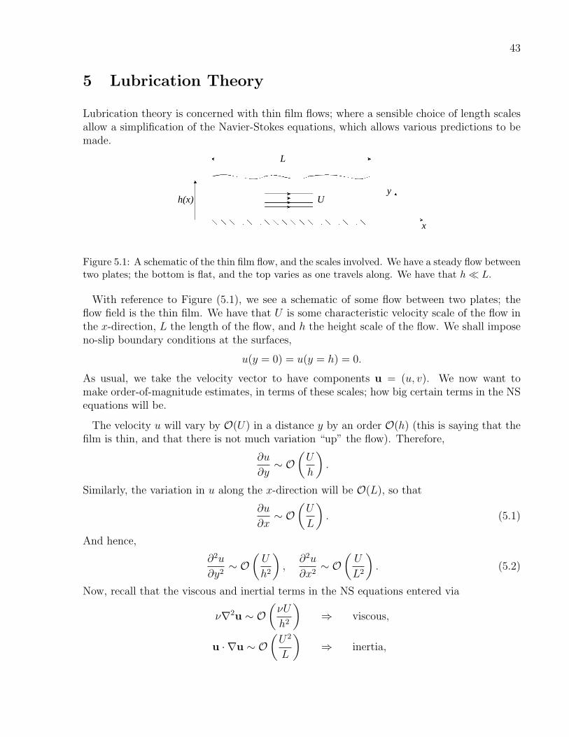
Lubrication theory is concerned with thin film flows; where a sensible choice of length scalesallow a simplification of the Navier-Stokes equations, which allows various predictions to bemade.

h(x) U

x

y

L

Figure 5.1: A schematic of the thin film flow, and the scales involved. We have a steady flow betweentwo plates; the bottom is flat, and the top varies as one travels along. We have that h L.

With reference to Figure (5.1), we see a schematic of some flow between two plates; theflow field is the thin film. We have that U is some characteristic velocity scale of the flow inthe x-direction, L the length of the flow, and h the height scale of the flow. We shall imposeno-slip boundary conditions at the surfaces,

u(y = 0) = u(y = h) = 0.

As usual, we take the velocity vector to have components u = (u, v). We now want tomake order-of-magnitude estimates, in terms of these scales; how big certain terms in the NSequations will be.

The velocity u will vary by O(U) in a distance y by an order O(h) (this is saying that thefilm is thin, and that there is not much variation “up” the flow). Therefore,

∂u

∂y∼ O

(U

h

).

Similarly, the variation in u along the x-direction will be O(L), so that

∂u

∂x∼ O

(U

L

). (5.1)

And hence,

∂2u

∂y2∼ O

(U

h2

),

∂2u

∂x2∼ O

(U

L2

). (5.2)

Now, recall that the viscous and inertial terms in the NS equations entered via

ν∇2u ∼ O(νU

h2

)⇒ viscous,

u · ∇u ∼ O(U2

L

)⇒ inertia,

44 5 LUBRICATION THEORY

after using (5.1) and (5.2); and hence in a comparison of inertia to viscous forces,

inertia

viscous∼ UL

ν

(h

L

)2

.

We can now notice that the first factor is the Reynolds number R, so that

inertia

viscous∼ R

(h

L

)2

. (5.3)

Recall that we could linearise the NS equations into the Stokes equations, in the limit thatR 1. This amounted to requiring viscous terms dominating over the inertia terms; andwe neglected the inertia terms. We now see that we can neglect the inertia terms in favourof the viscous terms, even if R is large, if h is very small (relative to L).

A common example of such a situation is when a sheet of paper slides over a surface. Takingthe speed scale to be U = 100mm s−1, the length of the sheet of paper L = 300mm, theheight of the paper above the surface over which it it sliding, h = 0.5mm and the viscosityof air ν = 15mm2s−1. Therefore, using these numbers,

R =UL

ν= 2000, R

(h

L

)2

= 0.05 1.

Therefore, we say that such a system is in the lubrication limit.

5.1 The Lubrication Equations

We shall now derive the lubrication equations, by considering the length scales in the NSequations, and noting which terms are negligible relative to others.

We shall now introduce some length and velocity scales,

x = Lx, y = hy, u = Uu, v = V v,

where all tilde-quantitities have the same scale, and actual scales are set by quantities suchas U,L. Upon substitution of the scale into the incompressibility condition,

∂u

∂x+∂v

∂y= 0,

we easily find thatU

L

∂u

∂x+V

h

∂v

∂y= 0.

The non-trivial solution of this only occurs if the pre-factors are of the same order,

U

L∼ V

h⇒ V ∼ hU

L.

5.2 Slider Bearing 45

Now let us scale the x-component of the NS equation,

u∂u

∂x+ v

∂u

∂y= −1

ρ

∂p

∂x+ ν

(∂2u

∂x2+∂2u

∂y2

).

Hence, putting in our scales,

U2u

L

∂u

∂x+hU2v

Lh

∂u

∂y= − P

ρL

∂p

∂x+νU

h2

(h2

L2

∂2u

∂x2+∂2u

∂y2

),

where we have introduced the pressure scale p = P p. Now, if h L, then h2/L2 1, sothat the second term on the RHS is negligible. Therefore, also dividing by the factor νU/h2,

1νUh2

U2

L

(u∂u

∂x+ v

∂u

∂y

)= − P

ρL

1νUh2

∂p

∂x+∂2u

∂y2,

rearranging slightly, easily gives(hU

ν

)h

Lu · ∇u = − Ph2

ρνLU

∂p

∂x+∂2u

∂y2.

Now, in the lubrication limit, the prefactor on the LHS is negligible (also, we stated previouslythat we want to neglect the inertia terms, which we have been able to show that we are allowedto do); also, the prefactor to the far RHS term is O(1). Therefore, to balance, we require

Ph2

ρνLU∼ O(1)

to balance this equation. This gives us a pressure scale P .

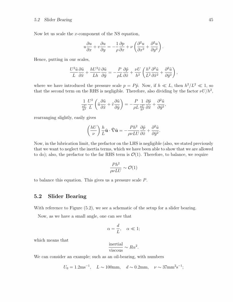
5.2 Slider Bearing

With reference to Figure (5.2), we see a schematic of the setup for a slider bearing.

Now, as we have a small angle, one can see that

α =d

L, α 1;

which means thatinertial

viscous∼ Rα2.

We can consider an example; such as an oil-bearing, with numbers

U0 = 1.2ms−1, L ∼ 100mm, d ∼ 0.2mm, ν ∼ 37mm2s−1;


d2

d1

d

U0

x = 0 x = L

B

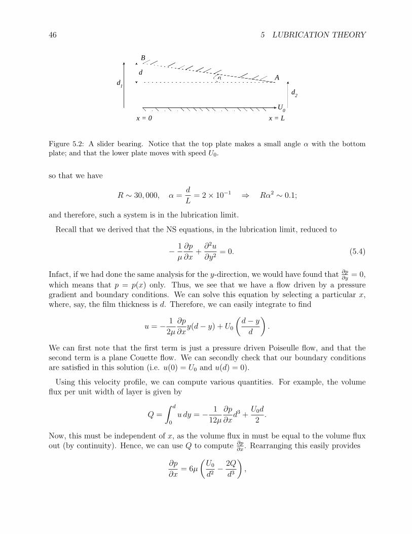
A

Figure 5.2: A slider bearing. Notice that the top plate makes a small angle α with the bottomplate; and that the lower plate moves with speed U0.

so that we have

R ∼ 30, 000, α =d

L= 2× 10−1 ⇒ Rα2 ∼ 0.1;

and therefore, such a system is in the lubrication limit.

Recall that we derived that the NS equations, in the lubrication limit, reduced to

− 1

µ

∂p

∂x+∂2u

∂y2= 0. (5.4)

Infact, if we had done the same analysis for the y-direction, we would have found that ∂p∂y

= 0,

which means that p = p(x) only. Thus, we see that we have a flow driven by a pressuregradient and boundary conditions. We can solve this equation by selecting a particular x,where, say, the film thickness is d. Therefore, we can easily integrate to find

u = − 1

2µ

∂p

∂xy(d− y) + U0

(d− yd

).

We can first note that the first term is just a pressure driven Poiseulle flow, and that thesecond term is a plane Couette flow. We can secondly check that our boundary conditionsare satisfied in this solution (i.e. u(0) = U0 and u(d) = 0).

Using this velocity profile, we can compute various quantities. For example, the volumeflux per unit width of layer is given by

Q =

∫ d

0

u dy = − 1

12µ

∂p

∂xd3 +

U0d

2.

Now, this must be independent of x, as the volume flux in must be equal to the volume fluxout (by continuity). Hence, we can use Q to compute ∂p

∂x. Rearranging this easily provides

∂p

∂x= 6µ

(U0

d2− 2Q

d3

),


noting that d ≡ d(x). So, we can integrate this, using the chain rule,

∂p

∂x=∂p

∂d

∂d

∂x,

where d(x) = d1 − αx, so that

∂p

∂d= −6µ

α

(U0

d2− 2Q

d3

).

Hence, integrating

p(d) =6µ

α

(U0

d− Q

d2

)+ C,

where C is a constant of integration. We can find C by imposing that at x = 0, we have apressure p = p0, and hence

p− p0 =6µ

α

[U0

(1

d− 1

d1

)−Q

(1

d2− 1

d21

)].

We could consider the case where the block is completely immersed in the fluid (for example,the paper is completely immersed in air). Then, the pressures at either end are the same, sothat p(d = d2) = p0. Hence,

Q = U0d1d2

d1 + d2

, (5.5)

p− p0 =6µU0

α

((d1 − d)(d− d2)

d2(d1 + d2)

). (5.6)

Although we shall not go through the details, one can compute further quantities;

• Total normal force (i.e. pressure generated by the flow):∫ L

0

p− p0 dx =6µU0

α2

[lnd1

d2

− 2

(d1 − d2

d1 + d2

)].

• Total tangential force exerted by the fluid on the lower plane:∫ L

0

µ∂u

∂y

∣∣∣∣y=0

dx =2µU0

α

[3

(d1 − d2

d1 + d2

)− 2 ln

d1

d2

].

• Total tangential force exerted by the fluid on the upper plane:

−∫ L

0

µ∂u

∂y

∣∣∣∣y=d

dx =2µU0

α

[3

(d1 − d2

d1 + d2

)− ln

d1

d2

].

The coefficient of friction is given by

coeff of friction =tangential force on block

normal force on block= αf

(d1

d2

),

where f(x) is some function. Now, if d1−d2d1∼ 1, then the coefficient of friction is ∼ d1/L,

which is very small. Therefore, the bearing has very low friction.


5.2.1 Cavitation

Consider that the pressure in an accelerated fluid is given by

p = p0 + ρ(g − β)h.

Now, notice that p < p0 occurs when β > g. That is, a negative pressure can occur if theacceleration is greater than that of gravity.

x/2

p − p0

p

Figure 5.3: The pressure profile under a thin film flow. Notice that there is a period of negativepressure; this corresponds to where the fluid vaporises and cavitation occurs.

With reference to Figure (5.3), we see the pressure profile under a thin film flow. Basically,what this negative pressure means, is that if the pressure difference drops below the vapourpressure of the fluid, then the fluid becomes a vapour. If this occurs in systems, then thewear-and-tear on such systems can be a very large effect.

Figure 5.4: A setup of how to generate cavitation in a fluid. Consider reducing the pressure abovethe fluid, to something quite close to the fluids vapour pressure. Then, if the tube is accelerateddownwards with acceleration β > g, the fluid will vaporise. When the tube is stopped, the vapourbubble collapses, making a loud noise and grinds away at the (reinforced) base.


With reference to Figure (5.4), we see a setup of how to generate cavitation. The pressuredifference p − p0 needed to allow water to cavitate, is 105Nm−2. Thus, taking h = 0.42mbelow the surface, an acceleration of β = 1.4g is needed.

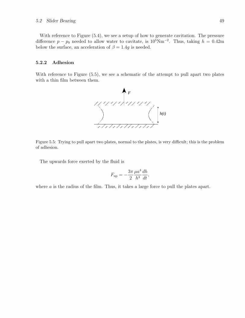
5.2.2 Adhesion

With reference to Figure (5.5), we see a schematic of the attempt to pull apart two plateswith a thin film between them.

F

h(t)

Figure 5.5: Trying to pull apart two plates, normal to the plates, is very difficult; this is the problemof adhesion.

The upwards force exerted by the fluid is

Fup = −3π

2

µa4

h3

dh

dt,

where a is the radius of the film. Thus, it takes a large force to pull the plates apart.


51

6 Aerofoil Theory

Consider a 2D aerofoil, as in Figure (6.1).

c

U0

pT , U

T

pB , U

B

Figure 6.1: An aerofoil in a flow.

We have an aerofoil with chord length c, in a flow of speed U0 and density ρ. The topof the wing has pressure and speed pT, UT, respectively. Similarly, the bottom of the winghas pB, UB. Notice that there is no drag on the wing, as the aerofoil is in a steady uniformirrotational flow.

The upward force per unit length on the elemental section is just

f = (pB − pT) dx.

Now, by Bernoulli, we have that

pB − pT =1

2ρ(U2

T − U2B

).

We can then write the RHS of this as an expansion,(U2

T − U2B

)= (UT − UB) (UT + UB) ,

and hence,

pB − pT =1

2ρ (UT − UB) (UT + UB) .

We now assume that the aerofoil is thin, so that

UT + UB ≈ 2U0,

and hence,pB − pT = ρU0 (UT − UB) .

Hence, the total lift per unit span is

L =

∫ c

0

f dx = ρU0

∫ c

0

UT − UB dx. (6.1)

52 6 AEROFOIL THEORY

high pressure

low pressure

Figure 6.2: An aerofoil in a flow, and the streamlines.

With reference to Figure (6.2), we see an exaggerated schematic of the streamlines aroundan aerofoil. Notice that above the wing, streamlines are close together, which means highspeed and low pressure. Equivalently, below the wing, streamlines are further apart, whichmeans low speed and high pressure. Therefore, there is a lift force perpendicular to thedirection of the flow.

6.1 Circulation

Consider defining

Γ =

∮C

u · dx, (6.2)

where C is some closed path in a fluid. Then, Γ is called the circulation. We can show thatan irrotational flow has zero circulation, by considering Stokes’ theorem,∮

C

u · dx =

∫S

(∇× u) · dS,

but ∇×u = 0 for an irrotational flow. And hence, the circulation Γ = 0 for irrotational flow.

Consider a closed path around the wing, so that

Γ =

∫ c

0

UBdx+

∫ 0

c

UTdx = −∫ c

0

(UT − UB) dx,

which is non-zero. Hence, upon comparison with our expression for lift, (6.1), we see that

L = −ρU0Γ. (6.3)

Therefore, we see that if we have lift, then we also therefore have circulation.

6.1 Circulation 53

(a) Flow with Γ = 0, resembles flow around a corner, atthe edge of the wing.

(b) Flow with Γ 6= 0, where there is a sharp separa-tion of the flow lines from the wing.

Figure 6.3: An aerofoil in a flow, and the streamlines.

The Joukowsi theorem states that any 2D object in an inviscid flow links lift and circulationin this way.

See Figure (6.3)a for a flow around an aerofoil for Γ = 0, which resembles a flow arounda corner, and requires a singular flow at the trailing edge. Figure (6.3)b is a flow withΓ = −L/ρU0, as we computed above. Viscosity helps in this case.

An interesting consequence of this, is Kelvin’s circulation theorm which states that for anyfluid governed by Euler’s equations, the circulation about a material loop is conserved;

D

Dt

∮u · d` = 0. (6.4)

Therefore, we have seen that lift implies a finite circulation, and that circulation is con-served. Hence, in order that circulation is conserved, an eddy of opposite circulation mustbe created when lift is initiated (and when lift is stopped) – this is a starting vortex. Thisvortex is created as a consequence of the fluid being primarily an inviscid flow field – i.e.persists for a very long time.

54 6 AEROFOIL THEORY

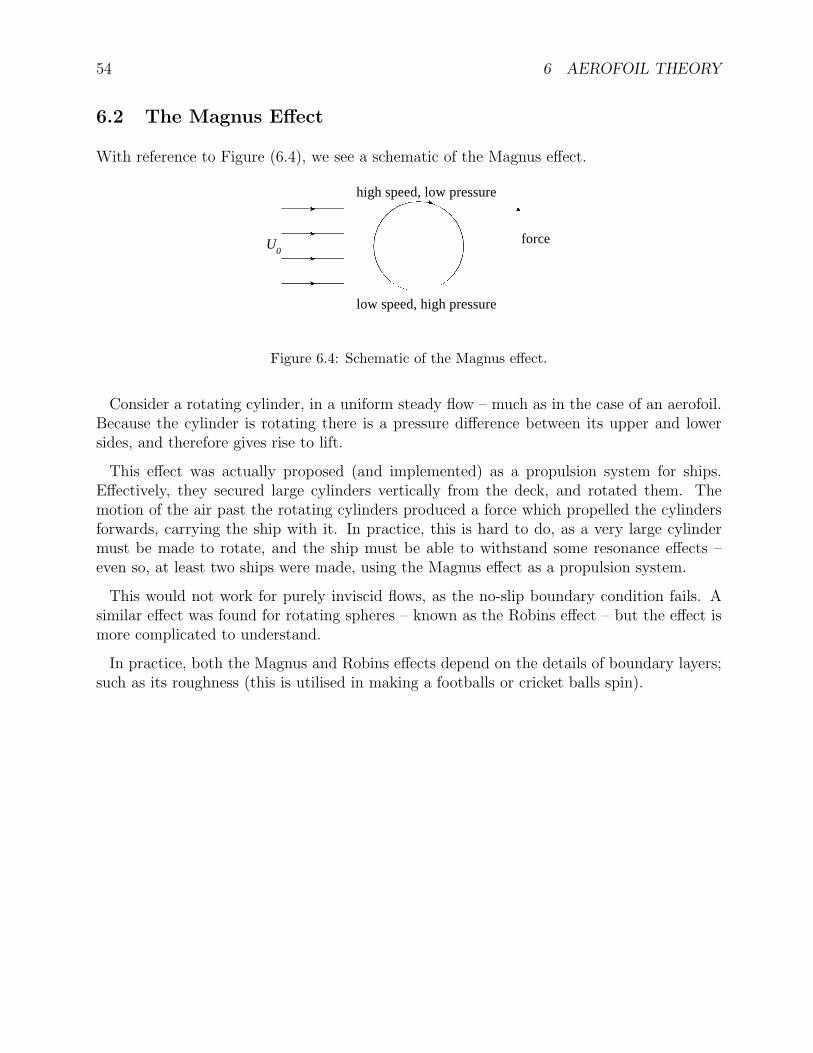
6.2 The Magnus Effect

With reference to Figure (6.4), we see a schematic of the Magnus effect.

force

high speed, low pressure

low speed, high pressure

U0

Figure 6.4: Schematic of the Magnus effect.

Consider a rotating cylinder, in a uniform steady flow – much as in the case of an aerofoil.Because the cylinder is rotating there is a pressure difference between its upper and lowersides, and therefore gives rise to lift.

This effect was actually proposed (and implemented) as a propulsion system for ships.Effectively, they secured large cylinders vertically from the deck, and rotated them. Themotion of the air past the rotating cylinders produced a force which propelled the cylindersforwards, carrying the ship with it. In practice, this is hard to do, as a very large cylindermust be made to rotate, and the ship must be able to withstand some resonance effects –even so, at least two ships were made, using the Magnus effect as a propulsion system.

This would not work for purely inviscid flows, as the no-slip boundary condition fails. Asimilar effect was found for rotating spheres – known as the Robins effect – but the effect ismore complicated to understand.

In practice, both the Magnus and Robins effects depend on the details of boundary layers;such as its roughness (this is utilised in making a footballs or cricket balls spin).

55

7 Boundary Layers

Eulers equations are a good approximation far from boundaries, as the Reynolds number Rgets very large. We rejected the no-slip boundary condition completely – with no gradualreduction as R increases. Now, experiment shows that no-slip is always important at bound-aries. The resolution of this required a new approach – the idea of a viscous boundary layer.Exactly as in the thin-film approach, we must carefully choose length scales.

A boundary layer is a region of concentrated vorticity which is long and thin. Vorticity isdiffused outwards slowly via the ν∇2ω-term, whilst being convected along by the u·∇ω-term,in the vorticity equation,

∂ω

∂t+ u · ∇ω = ω · ∇u + ν∇2ω. (7.1)

Boundaries are generators of vorticity, being regions of strong gradients of vorticity.

So, let us see where the consideration of scales gets us. Let L be the length scale of a body(such as the diameter of a cylinder, or length of a plate), and let δ be the viscous length scale– the boundary layer thickness. Hence, in the NS equations, we see that we can write thescales of the convective (i.e. inertia) and viscous terms;

u · ∇u ∼ O(U2

L

), ν∇2u ∼ O

(νU

δ2

).

Thus, the inertia and viscous terms will be of comparable order when

U2

L∼ νU

δ2,

which easily rearranges into

δ

L∼(UL

ν

)−1/2

=1√R.

Hence, the ratio of the boundary layer thickness to the length scale of the body is related tothe Reynolds number of the flow,

δ

L∼ 1√

R. (7.2)

For example, considering a 20mm diameter cylinder in a flow with R = 10, 000, there will bea boundary layer of thickness δ ∼ 0.2mm.

The outer flow – i.e. far from the boundary – either has a weak variation in vorticity, oris even irrotational. A solid body generates vorticity as it moves through the fluid (at highReynolds number), and carries the vorticity along with it.

The important difference with this and the Euler equations, is the addition of the viscosityterm ν ∂

2u∂y2

, which is due to a strong gradient of u in the direction normal to the body, andclose to it. For boundary layers this term can be very large.

56 7 BOUNDARY LAYERS

It is worth noting that boundary layer theory cannot be rigorously derived, merely hypoth-esised.

In practice, the edge of the boundary layer is often to be the position where the flow speedis very close to the outer flow speed, so y = δ where u = 0.99U0. The general idea is thatthe flow external to the boundary layer is given by a solution to Eulers equation, and thisprovides the outer boundary conditions for the layer.

(a) Ideal flow.

(b) Flow with boundary layer.

Figure 7.1: The velocity profiles past a thin plate. (a) shows the ideal flow, where the profile iscompletely unaffected by the plate; (b) shows a more realistic flow, where the passage of the flowpast a plate induces a boundary layer, and the velocity profile is disturbed. In case (b) we have awake forming because of the disturbance of the flow.

With reference to Figure (7.1), we see the difference in velocity profiles for ideal flow anda flow allowing a boundary layer, past a thin plate. With reference to Figure (7.2), we seethe velocity profiles for two types of flow past a sphere. The high R flow separates, forminga boundary layer, thickness δ.

7.1 2D Boundary Layers

Consider a 2D steady flow, as in Figure (7.3). We have length scales δ, L for the boundarylayer and length of body, respectively; and velocity scales U, V for the horizontal and verticaldirections, respectively.

Let us consider the appropriate scales in the NS equations.

7.1 2D Boundary Layers 57

U0

Figure 7.2: The difference in velocity profiles for inviscid (dotted line) and high R (dashed line)flows across a sphere. As the flow gets to the “edge” of the sphere, the flow will either continue ina straight line (i.e. the inviscid flow case) or will separate with some boundary layer δ.

x

y

L

UV

Figure 7.3: A 2D boundary layer, thickness δ, above a surface (at y = 0).

Recall (7.2), whereδ

L∼ 1√

R.

Now, the continuity equation∂u

∂x+∂v

∂y= 0,

has its terms having the scales

∼ U

L∼ V

δ,

and therefore we have

V ∼ Uδ

L. (7.3)

This is because the terms of the continuity equation must be of the same order, so that theyadd and cancel; since fluid entering the boundary layer must exit, even though the boundarylayer thickness is not constant. Therefore, (7.3) tells us that the flow speed “up”, V , is smallcompared to the flow speed “across”, U , when the boundary layer is thin (i.e. when δ is


small). We can use this to scale the NS equations. So, the x-component of the Navier-Stokesequations reads

u∂u

∂x+ v

∂u

∂y= −1

ρ

∂p

∂x+ ν

(∂2u

∂x2+∂2u

∂y2

),

after assuming steady flow. The first term is ∼ U2/L, the second term is ∼ V U/δ, fourthterm is ∼ νU/L2 and the fifth term ∼ νU/δ2. Using (7.3), we see that the order of the secondterm can be written ∼ V U/δ ∼ U2/L, which is the same order as the first term. Therefore,we see that the inertia terms balance. Now, V < U , but ∂u

∂y> ∂u

∂x. Therefore, we neglect the

fourth term relative to the fifth term (Notice that this can be seen due to L δ).

Now, outside of the boundary layer, we have our standard flow with

U0∂U0

∂x= −1

ρ

∂p0

∂x.

Therefore, the NS equations reduce to the boundary layer equations,

u∂u

∂x+ v

∂u

∂y= U0

dU0

dx+ ν

∂2u

∂y2, (7.4)

∂u

∂x+∂v

∂y= 0. (7.5)

Hence, we have two equations in two unknowns u, v. The equations can be solved if theouter-flow speed U0 is specified, so that the boundary conditions for the layer are found (i.e.solving Eulers equation for the free streaming outer-flow).

The solution to the boundary layer equations tends to be found by introducing a stream-function, and seeking similarity solution (that is, solutions with the same form for all x, butscales with y). This then gives a single non-linear equation, which is solved numerically.

There are three useful classifications for the boundary layer equations; three useful situa-tions.

Negative Pressure Gradient: Accelerating Flow Here we have a negative pressuregradient, and accelerating flow (i.e. the outer flow field has a reduction in pressure as you go“across”);

dU0

dx> 0,

dp0

dx< 0

This is called a favourable pressure gradient. See Figure (7.4) for an example. The reductionin pressure gradient above the layer means that the layer accelerates, and becomes thinner;the thickness is reduced downstream. Therefore, such a boundary layer flow is stable.

7.1 2D Boundary Layers 59

boundary layer

Figure 7.4: A 2D boundary layer, thickness δ; the flow in the boundary layer accelerates as thepressure gradient above the layer drops.

Zero Pressure Gradient This corresponds to a uniform outer-flow field, and hence auniform boundary layer – for example, flow over a flat plate, the so-called Blasius flow. Theboundary layer looks like Figure (7.3). The boundary conditions are u = v = 0 at y = 0 andu→ U0 as y/δ →∞. Now, recall that δ ∼ √ν. Hence, u→ U0 as y/ν1/2 →∞.

Positive Pressure Gradient Here consider

dU0

dx< 0,

dp0

dx> 0;

so that we have an adverse pressure gradient, and decelerated outer flow field. What happenshere, is that the boundary layer separates from the surface, and produces eddies. Theboundary layers thickness downstream thickens, meaning that the boundary layer is unstable.The boundary layer flow then modifies the Euler outer flow.


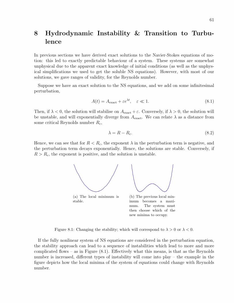
61

8 Hydrodynamic Instability & Transition to Turbu-

lence

In previous sections we have derived exact solutions to the Navier-Stokes equations of mo-tion: this led to exactly predictable behaviour of a system. These systems are somewhatunphysical due to the apparent exact knowledge of initial conditions (as well as the unphys-ical simplifications we used to get the soluble NS equations). However, with most of oursolutions, we gave ranges of validity, for the Reynolds number.

Suppose we have an exact solution to the NS equations, and we add on some infinitesimalperturbation,

A(t) = Aexact + εeλt, ε 1. (8.1)

Then, if λ < 0, the solution will stabilise on Aexact + ε. Conversely, if λ > 0, the solution willbe unstable, and will exponentially diverge from Aexact. We can relate λ as a distance fromsome critical Reynolds number Rc,

λ = R−Rc. (8.2)

Hence, we can see that for R < Rc, the exponent λ in the perturbation term is negative, andthe perturbation term decays exponentially. Hence, the solutions are stable. Conversely, ifR > Rc, the exponent is positive, and the solution is unstable.

(a) The local minimum isstable.

(b) The previous local min-imum becomes a maxi-mum. The system mustthen choose which of thenew minima to occupy.

Figure 8.1: Changing the stability; which will correspond to λ > 0 or λ < 0.

If the fully nonlinear system of NS equations are considered in the perturbation equation,the stability approach can lead to a sequence of instabilities which lead to more and morecomplicated flows – as in Figure (8.1). Effectively what this means, is that as the Reynoldsnumber is increased, different types of instability will come into play – the example in thefigure depicts how the local minima of the system of equations could change with Reynoldsnumber.

62 8 HYDRODYNAMIC INSTABILITY & TRANSITION TO TURBULENCE

Some approaches only consider linearised equations; in this case, only first order instabilityis strictly valid.

An example is flow past a cylinder. For R < 1, we get linear Stokes flow, where the flowlines are symmetric. As the Reynolds number is increased, 1 < R < 30, an asymmetric wakeforms. The general idea is this: as the Reynolds number is increased, past certain limits,new types of instabilities come into play. These instabilities effectively add new elements ofunpredictability. This loss of predictability is not due to a breakdown of the deterministic NSequations; for example, the non-linear oscillator problem is non-linear, and unpredictable,but the equations of motion are exact. The problem comes in the level of accuracy that theinitial conditions are known.

The long term unpredictability is chaos: an instability that becomes “amplified”.

We gain insight into turbulent flows by studying its origins using known exact solutions.This method does not always produce instabilities: circular Couette flow does, but planardoes not. Similarly, plane Poiseuille flow has an instability, but circular does not.

8.1 Linear Stability

We can analyse a simple model, devised by Landau and Stuart and Wilson. Their equationis

A = λA− A3, (8.3)

where A is the amplitude of the solution, which may be complex, and λ = R − Rc. So, letus consider steady solutions, with A = 0, and look at their stability. So, the above equationjust becomes

A(λ− A2) = 0.

This has two solutions: A = 0 or A = ±√λ. We now restrict ourselves to real amplitudes,A ∈ R. So, for A = 0, we have no restriction on λ. However, if A = ±√λ, we must havethat λ > 0.

We can plot these steady solutions on a bifurcation diagram, as in Figure (8.2). Withreference to the figure, we denote the solution A = 0 as the trivial solution, and we note thatnew non-trivial stable solutions exist for λ > 0. We have marked it on, but the solution withA = 0, λ > 0 is unstable.

In practice, one of the states will be preferred over the other, as in Figure (8.3). This couldbe the case if there is some imperfection in equipment, meaning that a ball will tend to rollone way rather than the other. This could be modeled by simply adding a constant to (8.3),so that A = λA− A3 + δ.

To test the stability of the trivial state, we add a perturbation to the static solution,

A(t) = 0 + ε(t),

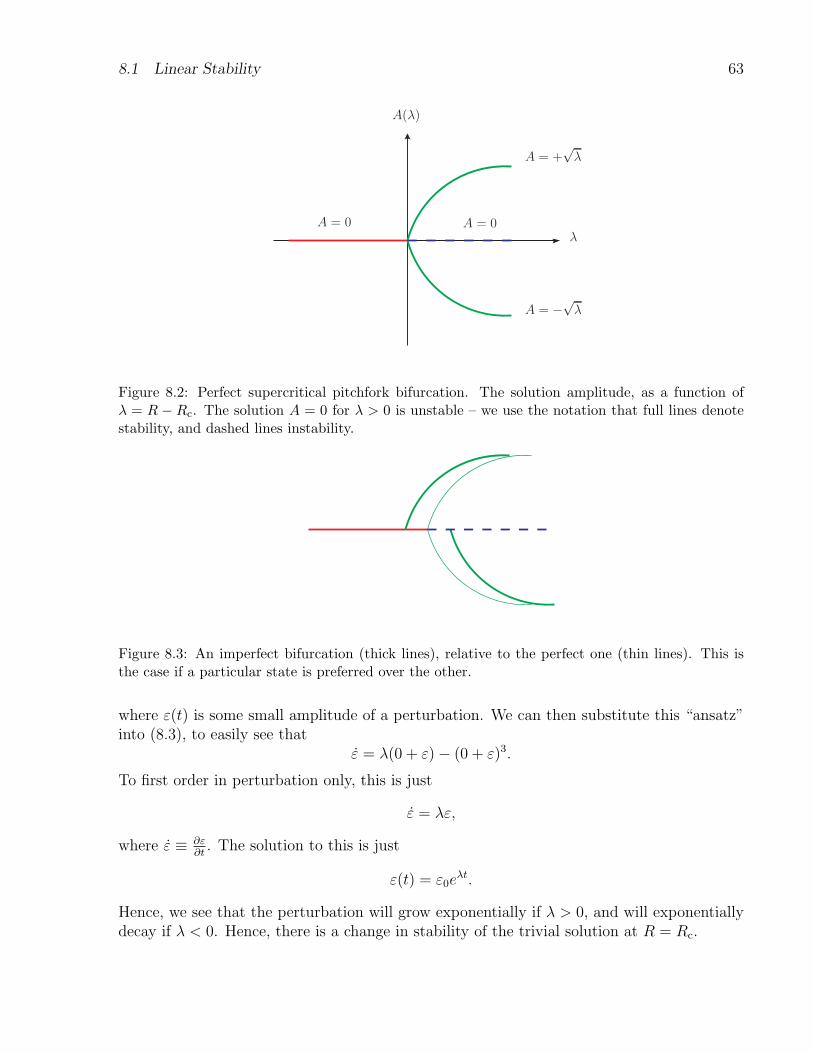
8.1 Linear Stability 63

A = +!

!

A = "!!

!

A(!)

A = 0 A = 0

Figure 8.2: Perfect supercritical pitchfork bifurcation. The solution amplitude, as a function ofλ = R − Rc. The solution A = 0 for λ > 0 is unstable – we use the notation that full lines denotestability, and dashed lines instability.

Figure 8.3: An imperfect bifurcation (thick lines), relative to the perfect one (thin lines). This isthe case if a particular state is preferred over the other.

where ε(t) is some small amplitude of a perturbation. We can then substitute this “ansatz”into (8.3), to easily see that

ε = λ(0 + ε)− (0 + ε)3.

To first order in perturbation only, this is just

ε = λε,

where ε ≡ ∂ε∂t

. The solution to this is just

ε(t) = ε0eλt.

Hence, we see that the perturbation will grow exponentially if λ > 0, and will exponentiallydecay if λ < 0. Hence, there is a change in stability of the trivial solution at R = Rc.


Let us test the stability of the A = +√λ solution. So, substituting into (8.3), we have

ε = λ(√

λ+ ε)−(√

λ+ ε)3

= λ3/2 + λε− λ3/2 − 3λε+O(ε2)

= −2λε.

Hence, the solution to this is just

ε(t) = ε0e−2λt, λ > 0.

This is an exponentially decaying solution. Therefore, the non-trivial√λ solution is linearly

stable (as can be similarly shown for the −√λ solution).

Therefore, our analysis of (8.3) has shown that there is an exchange of stability betweenthe trivial state and a pair of non-trivial states at R = Rc.

Let us consider a second model,

A = λA+ A3. (8.4)

Then, static solutions have amplitudes being the roots of

A(λ+ A2) = 0.

Hence, we easily see that we have the trivial state A = 0, and two non-trivial states A =±√−λ. Thus, for real amplitudes, we require λ < 0. So, let us have solution A(t) = A0+ε(t),where A0 is one of the three static solutions, and ε(t) is the amplitude of some time dependentperturbation from the solution. First consider the trivial solution, A0 = 0, so that uponsubstitution into (8.4), we have that

ε = ελ ⇒ ε(t) = ε0eλt.

Now, this describes a solution that is stable for λ < 0, and unstable for λ > 0. If we nowtake A0 = +

√−λ = i√λ, the equation (8.4) becomes (to first order in perturbation only),

ε = −2ελ ⇒ ε(t) = ε0e−2λt.

Now, these solutions only existed for λ < 0, and are hence always unstable.

See Figure (8.4) for the bifurcation diagram corresponding to this system.

Now, the bifurcation diagram for (8.4) shows that there are no stable solutions for A 6= 0.We can modify the equation into

A = λA+ A3 − A5, (8.5)

which, with reference to its diagram, Figure (8.5), we see that there exists stable solutionsfor A 6= 0. In this case, we see that for a given λ there can be 3 stable solutions.

8.1 Linear Stability 65

Figure 8.4: Subcritical pitchfork bifurcation describing the stability of solutions to (8.4).

Figure 8.5: Pitchfork bifurcation describing the stability of solutions to (8.5).

8.1.1 Hopf Bifurcation

In contrast to the pitchfork bifurcations, which gave rise to two stable solutions from asingle solution, the Hopf bifurcation gives rise to periodic oscillatory solutions from a steadysolution. This essentially corresponds to a periodic transition between the two states of thebifurcation.

Such a system of equations that has such a behaviour is

r = r(λ− r2), θ = ω. (8.6)

With reference to Figure (8.6), we see the Hopf bifurcation diagram; which is a singleperiodic orbit with frequency ω. Such a bifurcation can be realised by increasing the Reynoldsnumber R of a flow about a cylinder. At low R, the flow will be steady, but as R is increasedpast some Rc, the flow becomes oscillatory. Plane Poiseulle flow is an example of a subcriticalHopf bifurcation.


r

!

!""

""

Figure 8.6: The supercritical Hopf bifurcation diagram describing the system (8.6). Notice theperiodic oscillation between the two states.

8.2 Landau Theory for Onset of Turbulence

We have seen from our simple linear analysis that in passing some critical Reynolds number,a steady flow can become oscillatory. So we could consider the onset of turbulence – which isthe essentially random unpredictable motion of a fluid – as a result of passing many of thesetypes of critical values.

Let us propose that there is a critical Reynolds number Rc, such that at R = Rc, periodicinstability comes into affect, and grows as

|A|max ∝√R−Rc.

That is, the instability becomes greater in amplitude with Reynolds number. The corre-sponding velocity field is

u = f(x, y, z)e−i(ω1t+β1),

where ω1 is the first oscillatory frequency, and β1 is the initial phase. The Landau theory isthat as R is increased, there is a further instability with ω2, β2, and subsequent instabilitiesωi, βi; with each new frequency arising from a smaller increment in R, so that at some finiteR an infinite number of modes are excited with random phase. This infinite mode excitementis equivalent to turbulence.

See Figure (8.7) for a schematic view of the amplitude of instabilities in the Landau theory.Such a velocity distribution will then have

u(x, y, z) =∑n

An(x, y, z)e−iPnj=1(ωjt+βj). (8.7)

Hence, turbulence is an infinite sum over all possible modes, with a random phase. This isconsistent with the statistical description of turbulence.

We must ask however, is this viewpoint correct? Do all instances of the onset of turbulencein a fluid occur after an infinite sequence of instabilities (i.e. as in the Landau theory), or

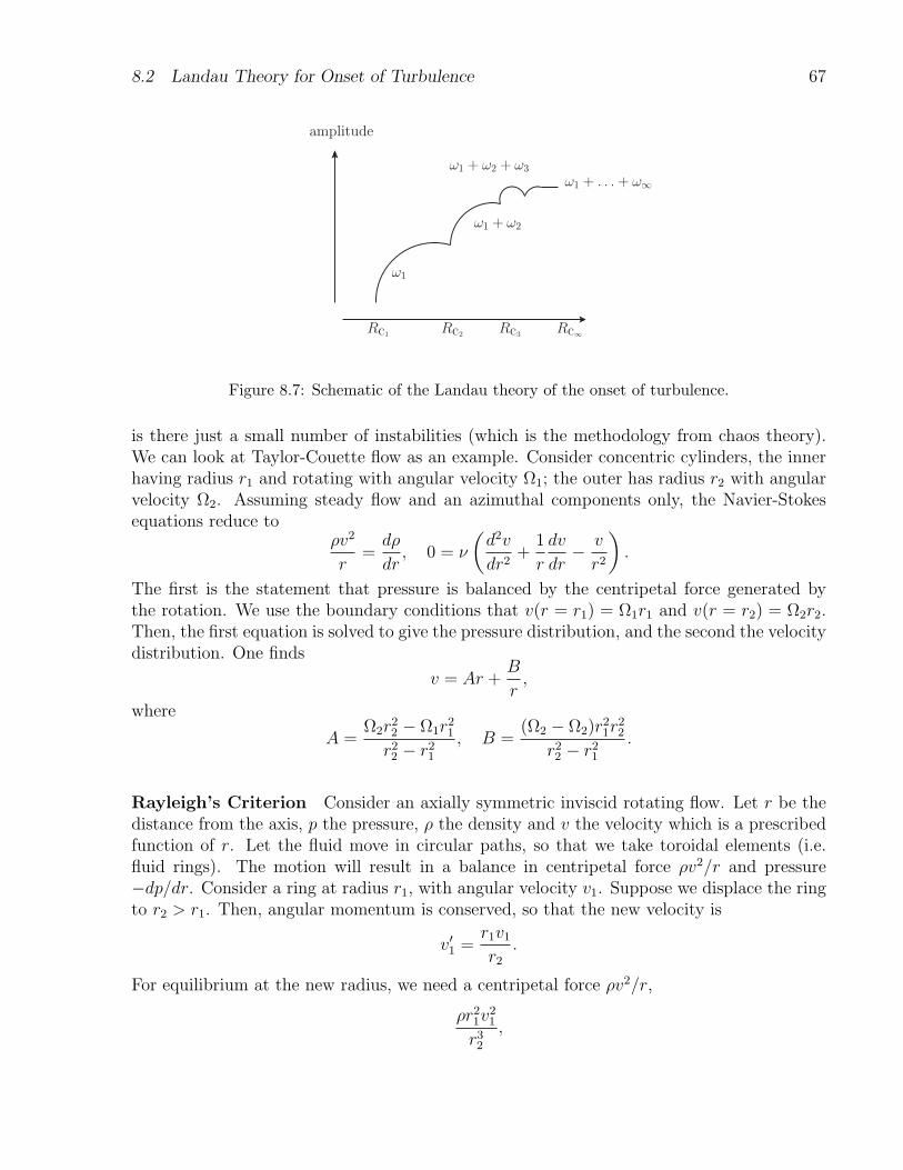
8.2 Landau Theory for Onset of Turbulence 67

Rc1Rc2

Rc3Rc!

!1

!1 + !2

!1 + !2 + !3!1 + . . . + !!

amplitude

Figure 8.7: Schematic of the Landau theory of the onset of turbulence.

is there just a small number of instabilities (which is the methodology from chaos theory).We can look at Taylor-Couette flow as an example. Consider concentric cylinders, the innerhaving radius r1 and rotating with angular velocity Ω1; the outer has radius r2 with angularvelocity Ω2. Assuming steady flow and an azimuthal components only, the Navier-Stokesequations reduce to

ρv2

r=dρ

dr, 0 = ν

(d2v

dr2+

1

r

dv

dr− v

r2

).

The first is the statement that pressure is balanced by the centripetal force generated bythe rotation. We use the boundary conditions that v(r = r1) = Ω1r1 and v(r = r2) = Ω2r2.Then, the first equation is solved to give the pressure distribution, and the second the velocitydistribution. One finds

v = Ar +B

r,

where

A =Ω2r

22 − Ω1r

21

r22 − r2

1

, B =(Ω2 − Ω2)r

21r

22

r22 − r2

1

.

Rayleigh’s Criterion Consider an axially symmetric inviscid rotating flow. Let r be thedistance from the axis, p the pressure, ρ the density and v the velocity which is a prescribedfunction of r. Let the fluid move in circular paths, so that we take toroidal elements (i.e.fluid rings). The motion will result in a balance in centripetal force ρv2/r and pressure−dp/dr. Consider a ring at radius r1, with angular velocity v1. Suppose we displace the ringto r2 > r1. Then, angular momentum is conserved, so that the new velocity is

v′1 =r1v1

r2.

For equilibrium at the new radius, we need a centripetal force ρv2/r,

ρr21v

21

r32

,


but, a pressure gradient at r2 supplies an inward force

ρv22

r2.

This, in general, is not equal to the centrifugal force required to balance the newly formedfluid ring. Thus, if

ρv22

r2>ρr2

1v21

r32

, (8.8)

the fluid ring will be forced back to where it came from. However, if

ρv22

r2<ρr2

1v21

r32

, (8.9)

the fluid ring will continue to move outwards.

Therefore, the flow is stable if (8.8) holds,

(r2v2)2 > (r1v1)

2, (8.10)

and unstable if (8.9) holds,

(r2v2)2 < (r1v1)

2. (8.11)

Notice that rv is infact the circulation of the flow. Therefore, we can now state Rayleigh’sCriterion:

A flow is stable if the square of the circulation increases outwards, and unstable if itdecreases outwards.

We can apply this to the rotating Couette flow. Let Ω1 and Ω2 denote the angular velocitiesof the inner and out cylinders, of radii r1, r2 respectively. If the cylinders rotate in the samedirection, the flow is unstable if (Ω1r1)

2 > (Ω2r2)2. For example, if the inner cylinder rotates

and the outer cylinder is stationary, the flow is always unstable. If the outer cylinder isstationary, and the gap between the cylinders is small, there is a linear shear problem. Theaction of viscosity is to stabilise the flow until the critical speed is reached.

Suppose we now make the cylinders rotate in opposite directions. Circulation now onlydecreases in part of the flow – this modifies the stability criterion into

d

dr|Ωr2| < 0 ⇐⇒ instability.

This can be seen in a system with translational invariance (such as infinite cylinders), wherethere will be multiple bifurcations; initially cells form, then Hopf bifurcations produce waveswithin the cells.

8.3 Turbulence 69

8.3 Turbulence

Chaos is a situation where a finite number of bifurcations are required for disorder – thisgives temporal disorder, and is not turbulence. The Landau theory stated that a infinitesequence of bifurcations leads to turbulence. Now, the idea of a sequence of instabilities doesnot always work – for rotary Taylor-Couette flow it does work, but for pipe flow or planeCouette flow, the idea does not work; both being linearly stable, but able to form disorderedflow.

The problem of turbulence is often called the last great unsolved problem of classicalphysics, and is of fundamental importance as most flows are turbulent – as a simple example,flow from a tap. The nature of the problem forces a descriptive description. If the flow rateis small, the laminar flow is smooth, and is a derivable exact solution of the NS equations.However, if the flow rate is increased, there is a sudden transition to turbulent (rough) flow– so rough, an empirical description is required. We could ask however, if the Reynoldsnumber is increased far enough, does the flow become completely random – the answer,fairly obviously, is no.

The probability distribution of the is non-Gaussian, but the flow is not completely random,as it contains structures (such as eddies). Thus, statistical properties are useful, such as themean velocity distribution.

Ideas can be explored using the special case of grid generated turbulence, whereby a regulargrid is moved through a fluid. Suppose we have a grid with spacing m. Then, initial eddiesof size m cascade down to smaller eddies as they flow. Consider in Fourier space – the energyis initially at large scales, but changes to smaller scales – an inertial range of scales.

8.3.1 Energy Cascade

The general idea for how big eddies supply energy to smaller eddies is this. Energy istransfered down from large to small eddies, until the action of viscosity on the smallest scales– kd. Large eddies interact with mean flow; for example, in a pipe of radius r, driven bymean flow, dissipating eddies are of order 0.01r. The transfer of energy takes place via vortexstretching, which is a 3D process. Viscosity is relatively unimportant in turbulent flows. Thephysical mechanisms of energy transfer in turbulence is:

• Cascade of instabilities: energy large to smaller scales, giving rise to greater complexity.

• Small scales extract energy from mean flow.

• Vortex lines stretch, increasing vorticity, and tangle; hence, a loss of predictability.


We can consider the flow field as u + uf , where the first term is a mean velocity and thesecond the fluctuations. This gives rise to an extra self-interaction term in the NS equation,

uf∂uf∂x

.

8.4 The Kolmogorov Spectrum

An hypothesis for dealing with the energy cascade comes from a fairly simple dimensionalanalysis.

Consider a energy spectrum E(k) as a function of wavenumber k in the inertial range(i.e. on small scales). Then, E(k)dk is the average turbulent energy per unit mass betweenk → k + dk. To get a feel for E(k), suppose we define the kinetic energy per unit volume,

Φ ≡ 1

2ρq2,

where the average velocity is

q2 = u2 + v2 + w2.

Hence,Φ

ρ=

1

2q2 =

∫ ∞0

E(k) dk.

The dimensions of E(k) can be computed quite simply,

[E] =[q2]

[k]=L2T−2

L−1= L3T−2.

Now, suppose we define the energy dissipation E , which is the energy flow per unit mass perunit time (i.e. down the scales in inertial range, until reach k−1

d , the size of fluid elementsthemselves). Thus, by dimensions, we have

[E ] = ML2T−2T−1M−1 = L2T−3.

We now assume that the dependence of E(k) upon E and k is

E(E , k) = CEαkβ,

where we can deduce α and β via dimensional arguments,

[E] = [E ]α[k]β.

Hence,

L3T−2 = (L2T−3)α(L−1)β,

8.5 Reynolds Stresses 71

so by equating the exponents of L and T , we can easily see that

α =2

3, β = −5

3.

Therefore,

E(E , k) = CE2/3k−5/3, (8.12)

where C is a dimensionless constant. This has been confirmed by experiment, and atmo-spheric flow experiments have found that C = 1.5. The agreement is not perfect at high k(i.e. very small scales), where there is no real consensus as to a reason.

There is a subtlety with this. Dissipation is not isotropic at small scales, as we assumedabove.

8.5 Reynolds Stresses

Our aim is to show that small fluctuations lead to large flow resistance in turbulent flows viaReynolds stresses.

Consider an infinitesimal block of fluid, dxdydz. Then, the rate at which the x-componentof momentum passes through dydz is the mass flux times the velocity,

= ρUdydzU.

Now, in turbulent flow, we represent the motion as an averge plus some fluctuation whichdoes not have an average,

U = u+ uf ,

where uf = 0. Hence, the above expression for momentum rate becomes

ρUdydzU = ρU2dydz

= ρ(u+ uf )2dydz

= ρ(u2 + 2uuf + u2f )dydz,

but taking the average of this quantity removes the middle term from the brackets,

ρ(u2 + u2f )dydz.

Therefore, we see that the rate of momentum has an additional term due to the fluctuationswith zero mean. The point of this extra term is that the non-linear term in the NS equationsgets modified, to give extra stresses the so-called Reynolds stresses: ∼ ρU2.

In pipe flow, experiment tells us that turbulent fluctuations are ≈ ±10% about the mean.Hence, the Reynolds stresses are ≈ 0.001ρU2. Velocity gradients in a pipe are ∼ U/r, so thatviscous stresses are ∼ µU/r. Hence, the ratio is

Reynolds stresses

viscous stresses= 0.001

Ur

ν= 0.001R.


Thus, for a flow with R = 106, the Reynolds stresses are about 1000 times the viscousstresses.

Documents

Physics of Fluids - · PDF filePhysics of Fluids J.Pearson May 26, 2009 Abstract These are a set of notes I have made, based on lectures given by T.Mullin at the Uni-versity of Manchester