Physics Laboratory

Introduction and Support Materials

PHYC 20080 Fields, Waves and Light

Autumn 2021

2

Contents

Introduction 3

About Laboratory Schedule 4

Grading Process and Lab Rules 4

UCD plagiarism statement 5

Summary on Uncertainties 6

Graphing 8

Example Report Springs 10

Lab Scripts Lab scripts are supplied in print at the start of each lab. These are also made available online on the school of physics pages. In advance of each lab, read through the respective lab script and have a go at its warmup exercises. Consider this introduction and its appendices to be part of each lab script. So bring this to each lab.

3

Introduction Physics is an experimental science. The theory that is presented in lectures has its origins in, and is validated by, experiment.

Laboratories are staged through the semester in parallel to the lectures. They serve the following purposes:

• an opportunity to independently test theories by genuine observation;

• a means to enrich understanding of physical concepts presented in lectures;

• an opportunity to develop experimental techniques, skills of data analysis, the understanding of experimental uncertainty, and the development of graphical visualisation of data.

Based on these skills, you are expected to present experimental results in a logical fashion (graphically and in calculations), to use units correctly and consistently, and to plot graphs with appropriate axis labels and scales. You will have to draw clear conclusions (as briefly as possible) from the experimental investigations, on what are the major findings of each experiment and whetever or not they are consistent with your predictions. You should also demonstrate an appreciation of the concept of experimental uncertainty and estimate its impact on the final result.

Some of the experiments in the manual may appear similar to those at school, but the emphasis and expectations are likely to be different. Do not treat this manual as a ‘cooking recipe’ where you follow a prescription. Instead, understand what it is you are doing, why you are asked to plot certain quantities, and how experimental uncertainties affect your results. It is more important to understand and show your understanding in the write-ups than it is to rush through each experiment ticking the boxes. This manual includes blanks for entering most of your observations. Additional space is included at the end of each experiment for other relevant information. All data, observations and conclusions should be entered in this manual. Graphs may be produced by hand or electronically (details of a simple computer package are provided) and should be secured to this manual.

4

Laboratory Schedule

Students will be assigned to one of a number of groups and must attend at a specified time on Tuesday or Thursday afternoons. A detailed schedule is available online for you to find out which group you are in. In total you will perform six experiments during the semester. Students seeking guidance on the format expected for practical reports for PHYC20080 are referred to the back of this manual where an example report for an experiment on springs, designed to introduce students to Hooke’s law and graphing experimental data, is included. Reports can be typed or handwritten.

Lab Rules

1. No eating or drinking.

2. Bags and belongings are placed on the shelves provided in the labs.

3. It is the student’s responsibility to attend all SISWeb (UCD calendar) scheduled labs.

Zero grade is assigned by default for not attending a scheduled lab. Should you miss

a scheduled lab, raise this to your coordinator as soon as you are able.

4. Students work individually and reports are prepared individually. You must comply

with UCD plagiarism policy (see next page).

5. Covid-related. All labs require your physical attendance. Bring a face mask to all

labs. We adhere to safety measures put in place by UCD with regards to Covid.

5

UCD Plagiarism Statement

(taken from http://www.ucd.ie/registry/academicsecretariat/docs/plagiarism_po.pdf)

The creation of knowledge and wider understanding in all academic disciplines depends on building from existing sources of knowledge. The University upholds the principle of academic integrity, whereby appropriate acknowledgement is given to the contributions of others in any work, through appropriate internal citations and references. Students should be aware that good referencing is integral to the study of any subject and part of good academic practice.

The University understands plagiarism to be the inclusion of another person’s writings or ideas or works, in any formally presented work (including essays, theses, projects, laboratory reports, examinations, oral, poster or slide presentations) which form part of the assessment requirements for a module or programme of study, without due acknowledgement either wholly or in part of the original source of the material through appropriate citation. Plagiarism is a form of academic dishonesty, where ideas are presented falsely, either implicitly or explicitly, as being the original thought of the author’s. The presentation of work, which contains the ideas, or work of others without appropriate attribution and citation, (other than information that can be generally accepted to be common knowledge which is generally known and does not require to be formally cited in a written piece of work) is an act of plagiarism. It can include the following:

1. Presenting work authored by a third party, including other students, friends, family, or work purchased through internet services;

2. Presenting work copied extensively with only minor textual changes from the internet, books, journals or any other source;

3. Improper paraphrasing, where a passage or idea is summarised without due acknowledgement of the original source;

4. Failing to include citation of all original sources; 5. Representing collaborative work as one’s own;

Plagiarism is a serious academic offence. While plagiarism may be easy to commit unintentionally, it is defined by the act not the intention. All students are responsible for being familiar with the University’s policy statement on plagiarism and are encouraged, if in doubt, to seek guidance from an academic member of staff. The University advocates a developmental approach to plagiarism and encourages students to adopt good academic practice by maintaining academic integrity in the presentation of all academic work.

6

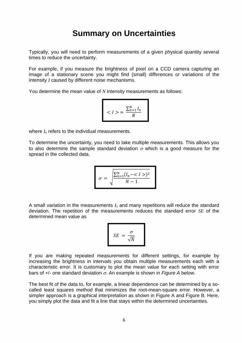
Summary on Uncertainties Typically, you will need to perform measurements of a given physical quantity several times to reduce the uncertainty. For example, if you measure the brightness of pixel on a CCD camera capturing an image of a stationary scene you might find (small) differences or variations of the intensity I caused by different noise mechanisms. You determine the mean value of N intensity measurements as follows:

< 𝐼 > = ∑ 𝐼𝑛

𝑁𝑛=1

𝑁

where In refers to the individual measurements. To determine the uncertainty, you need to take multiple measurements. This allows you

to also determine the sample standard deviation which is a good measure for the spread in the collected data.

= √∑ (𝐼𝑛−< 𝐼 >)2𝑁

𝑛=1

𝑁 − 1

A small variation in the measurements In and many repetitions will reduce the standard deviation. The repetition of the measurements reduces the standard error SE of the determined mean value as

𝑆𝐸 =

√𝑁

If you are making repeated measurements for different settings, for example by increasing the brightness in intervals you obtain multiple measurements each with a characteristic error. It is customary to plot the mean value for each setting with error

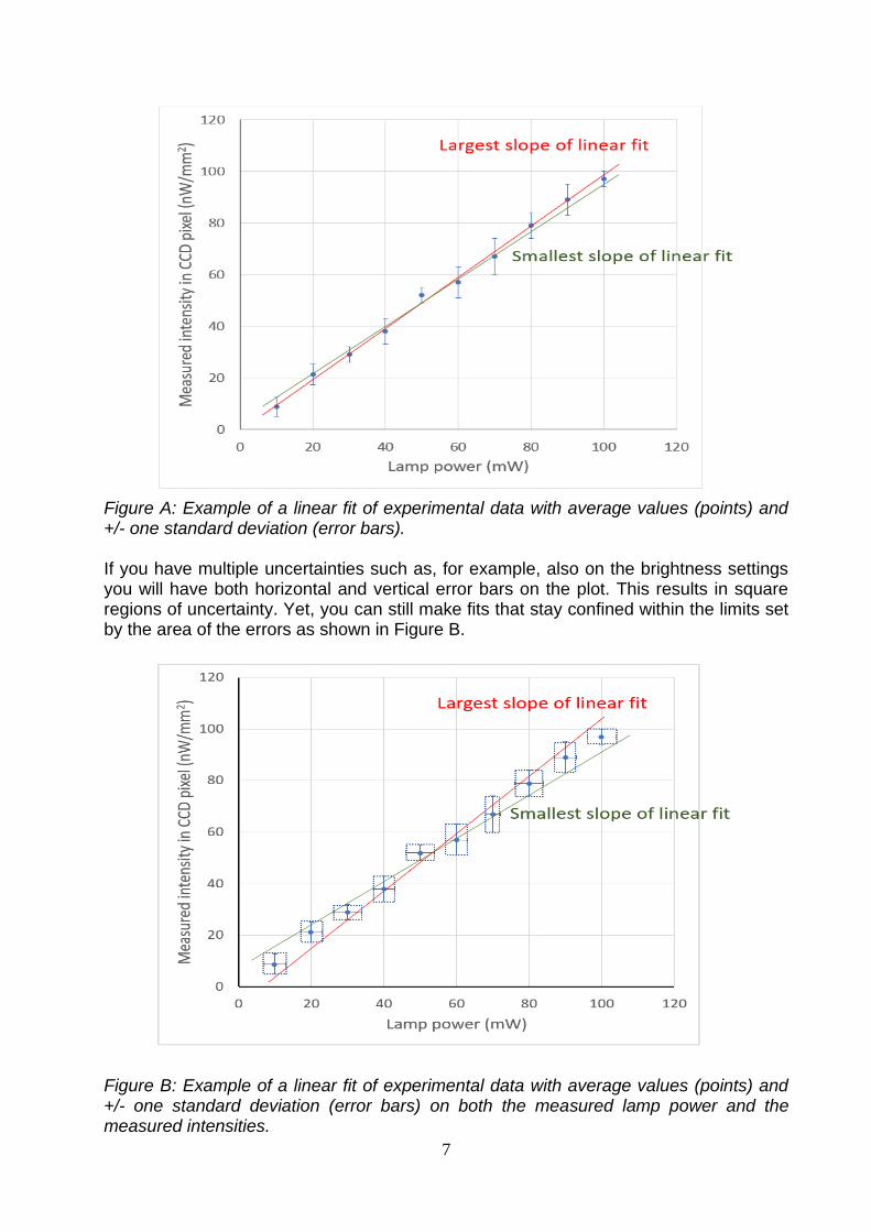
bars of +/- one standard deviation . An example is shown in Figure A below. The best fit of the data to, for example, a linear dependence can be determined by a so-called least squares method that minimizes the root-mean-square error. However, a simpler approach is a graphical interpretation as shown in Figure A and Figure B. Here, you simply plot the data and fit a line that stays within the determined uncertainties.

7

Figure A: Example of a linear fit of experimental data with average values (points) and +/- one standard deviation (error bars). If you have multiple uncertainties such as, for example, also on the brightness settings you will have both horizontal and vertical error bars on the plot. This results in square regions of uncertainty. Yet, you can still make fits that stay confined within the limits set by the area of the errors as shown in Figure B.

Figure B: Example of a linear fit of experimental data with average values (points) and +/- one standard deviation (error bars) on both the measured lamp power and the measured intensities.

8

Graphing Many of the experiments in this laboratory involve the plotting of a graph. Graphs are very important in Physics as they provide a simple display of the results obtained in an experiment and of the relationship between two variables. More accurate and reliable information can be obtained from a graph than from the analysis of any particular set of results. Plotting graphs by hand: (1) Scale: It is important to choose the scales so as to make full use of the squared

page. The scale divisions should be chosen for convenience; that is, one unit is either 1, 2 or 5 times a power of ten e.g. 0.5, 5, 100 etc., but never 3, 7, 9 etc.

(2) Marking the points: Readings should be indicated on the graph by a ringed dot and drawn with pencil, so that it is possible to erase and correct any unsatisfactory data.

(3) Joining the points: In the case of a straight line which indicates a direct proportion

between the variables, the ruler is positioned so that the line drawn will pass through as many points as possible. Those points which do not lie on the line should be equally distributed on both sides of the line. A point which lies away from this line can be regarded as ‘doubtful’ and a recheck made on the readings. In the case of a curve, the individual experimental points are not joined with straight lines but a smooth curve is drawn through them so that as many as possible lie on the curve.

(4) Units: The graph is drawn on squared page. Each graph should carry title at the

top e.g. Time squared vs. Length. The axes should be labelled with the name and units of the quantities involved.

(5) In the case of a straight-line graph, the equation of the line representing the

relationship between the quantities x and y may be expressed in the form y = mx + c where m is the slope of the line and c the intercept on the y-axis. The slope may

be positive or negative. Many experiments require an accurate reading of the slope of a line.

9

Using JagFit

In the examples above we have somewhat causally referred to the ‘best fit’ through the data. What we mean by this, is the theoretical curve which comes closest to the data points having due regard for the experimental uncertainties. This is more or less what you tried to do by eye, but how could you tell that you indeed did have the best fit and what method did you use to work out statistical uncertainties on the slope and intercept? The theoretical curve which comes closest to the data points having due regard for the experimental uncertainties can be defined more rigorously1 and the mathematical definition in the footnote allows you to calculate explicitly what the best fit would be for a given data set and theoretical model. However, the mathematics is tricky and tedious, as is drawing plots by hand and for that reason.... We can use a computer to speed up the plotting of experimental data and to improve the precision of parameter estimation.

In the laboratories a plotting programme called Jagfit is installed on the computers. Jagfit is freely available for download from this address: http://www.southalabama.edu/physics/software/software.htm

Double-click on the JagFit icon to start the program. The working of JagFit is fairly intuitive. Enter your data in the columns on the left.

• Under Graph, select the columns to graph, and the name for the axes.

• Under Error Method, you can include uncertainties on the points.

• Under Tools, you can fit the data using a function as defined under Fitting_Function. Normally you will just perform a linear fit.

1 If you want to know more about this equation, why it works, or how to solve it, ask your

demonstrator or read about ‘least square fitting’ in a text book on data analysis or statistics.

10

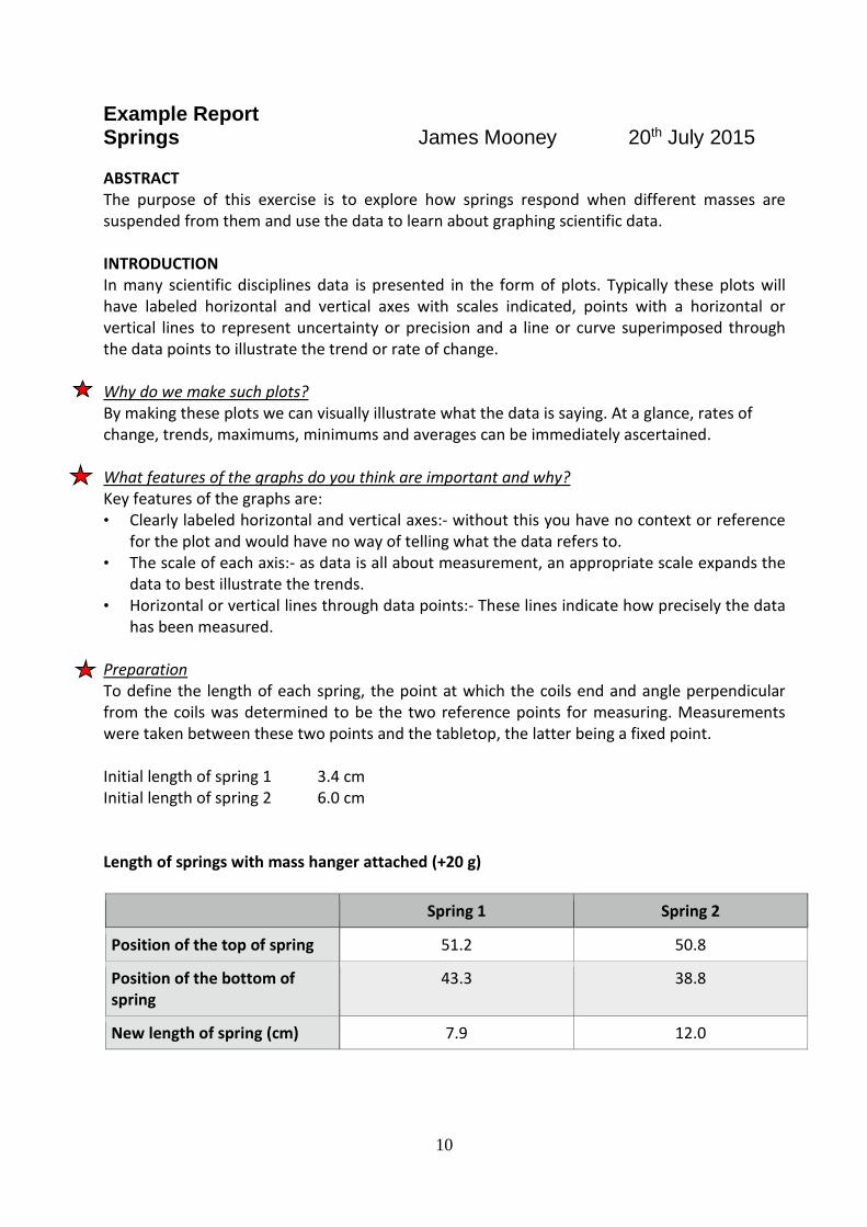
Example Report Springs James Mooney 20th July 2015

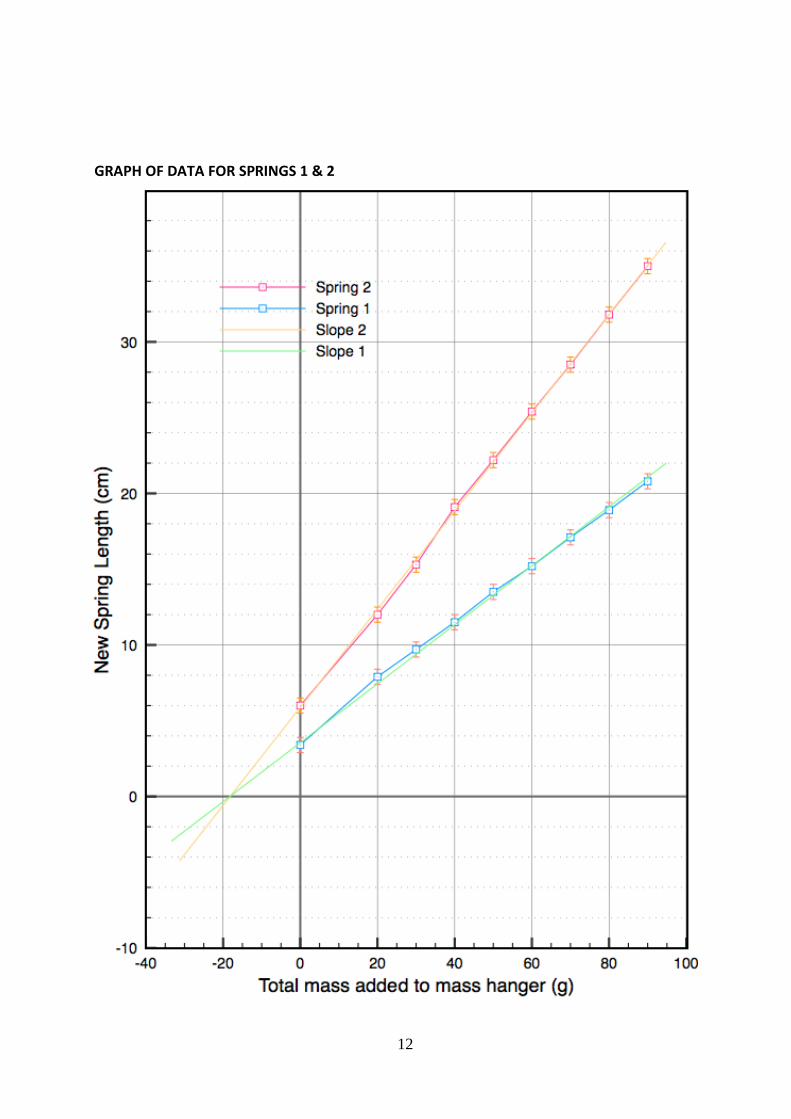
ABSTRACT The purpose of this exercise is to explore how springs respond when different masses are suspended from them and use the data to learn about graphing scientific data. INTRODUCTION In many scientific disciplines data is presented in the form of plots. Typically these plots will have labeled horizontal and vertical axes with scales indicated, points with a horizontal or vertical lines to represent uncertainty or precision and a line or curve superimposed through the data points to illustrate the trend or rate of change. Why do we make such plots? By making these plots we can visually illustrate what the data is saying. At a glance, rates of change, trends, maximums, minimums and averages can be immediately ascertained. What features of the graphs do you think are important and why? Key features of the graphs are: • Clearly labeled horizontal and vertical axes:- without this you have no context or reference

for the plot and would have no way of telling what the data refers to. • The scale of each axis:- as data is all about measurement, an appropriate scale expands the

data to best illustrate the trends. • Horizontal or vertical lines through data points:- These lines indicate how precisely the data

has been measured. Preparation To define the length of each spring, the point at which the coils end and angle perpendicular from the coils was determined to be the two reference points for measuring. Measurements were taken between these two points and the tabletop, the latter being a fixed point. Initial length of spring 1 3.4 cm Initial length of spring 2 6.0 cm Length of springs with mass hanger attached (+20 g)

Spring 1 Spring 2

Position of the top of spring 51.2 50.8

Position of the bottom of spring

43.3 38.8

New length of spring (cm) 7.9 12.0

11

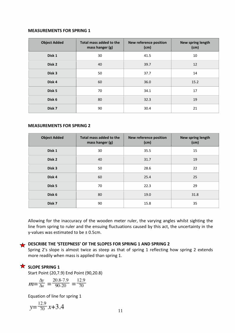
MEASUREMENTS FOR SPRING 1

Object Added Total mass added to the mass hanger (g)

New reference position (cm)

New spring length (cm)

Disk 1 30 41.5 10

Disk 2 40 39.7 12

Disk 3 50 37.7 14

Disk 4 60 36.0 15.2

Disk 5 70 34.1 17

Disk 6 80 32.3 19

Disk 7 90 30.4 21

MEASUREMENTS FOR SPRING 2

Object Added Total mass added to the mass hanger (g)

New reference position (cm)

New spring length (cm)

Disk 1 30 35.5 15

Disk 2 40 31.7 19

Disk 3 50 28.6 22

Disk 4 60 25.4 25

Disk 5 70 22.3 29

Disk 6 80 19.0 31.8

Disk 7 90 15.8 35

Allowing for the inaccuracy of the wooden meter ruler, the varying angles whilst sighting the line from spring to ruler and the ensuing fluctuations caused by this act, the uncertainty in the y-values was estimated to be ± 0.5cm. DESCRIBE THE ‘STEEPNESS’ OF THE SLOPES FOR SPRING 1 AND SPRING 2 Spring 2’s slope is almost twice as steep as that of spring 1 reflecting how spring 2 extends more readily when mass is applied than spring 1. SLOPE SPRING 1 Start Point (20,7.9) End Point (90,20.8)

Equation of line for spring 1

12

GRAPH OF DATA FOR SPRINGS 1 & 2

13

SLOPE SPRING 2 Start Point (20,12) End Point (90,35)

Equation of line for spring 2

WHAT ARE THE TWO INTERCEPTS? Spring 1: when x=0, y is 3.4. Spring 2: when x=0, y is 6. These are the lengths of the springs measured before adding any weights. HOW CAN YOU USE THE SLOPES OF THE TWO LINES TO COMPARE THE STIFFNESS OF THE SPRINGS? The slopes illustrate that spring 1 is almost twice as stiff as spring 2 CONCLUSION The linear behaviour of springs is clearly illustrated by the graph of the data depicting the correlation between the length of each spring and the mass added. This demonstrates Hooke’s law, which states that the extension produced is proportional to the force applied. In this case the force on the spring is proportional to the mass added. Within the experimental uncertainties the graphs for the two springs are consistent with this law. The graph shows that spring 1 is stiffer than spring 2.