Embed Size (px)
Citation preview

International Journal of Computer Vision, 2009DOI: 10.1007/s11263-009-0274-5
Physics-Based Person Tracking Using TheAnthropomorphic Walker
Marcus A. Brubaker · David J. Fleet · Aaron Hertzmann
Received: March 2008 / Accepted: July 2009
Abstract We introduce a physics-based model for 3Dperson tracking. Based on a biomechanical characteri-
zation of lower-body dynamics, the model captures im-
portant physical properties of bipedal locomotion such
as balance and ground contact. The model generalizesnaturally to variations in style due to changes in speed,
step-length, and mass, and avoids common problems
(such as footskate) that arise with existing trackers. The
dynamics comprise a two degree-of-freedom represen-
tation of human locomotion with inelastic ground con-tact. A stochastic controller generates impulsive forces
during the toe-off stage of walking, and spring-like forces
between the legs. A higher-dimensional kinematic body
model is conditioned on the underlying dynamics. The
This work was financially supported in part by NSERC Canada,the Canadian Institute for Advanced Research (CIFAR), theCanada Foundation for Innovation (CFI), the Alfred P. SloanFoundation, Microsoft Research and the Ontario Ministry of Re-search and Innovation. A preliminary version of this work ap-
peared in [5].
Marcus A. BrubakerDepartment of Computer ScienceUniversity of TorontoTel.: 416 946 8485Fax: 416 978 1455E-mail: [email protected]
David J. FleetDepartment of Computer ScienceUniversity of TorontoTel.: 416 946 8485Fax: 416 978 1455E-mail: [email protected]
Aaron HertzmannDepartment of Computer ScienceUniversity of TorontoTel.: 416 946 8497Fax: 416 978 1455E-mail: [email protected]
combined model is used to track walking people in video,including examples with turning, occlusion, and vary-
ing gait. We also report quantitative monocular and
binocular tracking results with the HumanEva dataset.
Keywords Tracking People · Physics · Passive-BasedWalking
1 Introduction
Most current methods for recovering human motion
from monocular video rely on kinematic models learned
from motion capture (mocap) data. Generative approaches
rely on density estimation to learn a prior distribution
over plausible human poses and motions, whereas dis-criminative models typically learn a mapping from im-
age measurements to 3D pose. While the use of learned
kinematic models clearly reduces ambiguities in pose
estimation and tracking, the 3D motions estimated bythese methods are often physically implausible. The
most common artifacts include jerky motions, feet that
slide when in contact with the ground (or float above
it), and out-of-plane rotations that violate balance.
The problem is, in part, due to the relatively smallamount of available training data, and, in part, due to
the limited ability of such models to generalize well be-
yond the training data. For example, a model trained on
walking with a short stride may have difficulty tracking
and reconstructing the motion of someone walking witha long stride or at a very different speed. Indeed, hu-
man motion depends significantly on a wide variety of
factors including speed, step length, ground slope, ter-
rain variability, ground friction, and variations in bodymass distributions. The task of gathering enough mo-
tion capture data to span all these conditions, and gen-
eralize sufficiently well, is prohibitive.
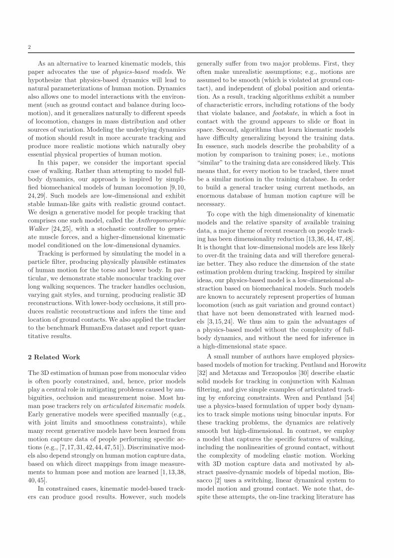
2
As an alternative to learned kinematic models, this
paper advocates the use of physics-based models. We
hypothesize that physics-based dynamics will lead to
natural parameterizations of human motion. Dynamics
also allows one to model interactions with the environ-ment (such as ground contact and balance during loco-
motion), and it generalizes naturally to different speeds
of locomotion, changes in mass distribution and other
sources of variation. Modeling the underlying dynamicsof motion should result in more accurate tracking and
produce more realistic motions which naturally obey
essential physical properties of human motion.
In this paper, we consider the important special
case of walking. Rather than attempting to model full-body dynamics, our approach is inspired by simpli-
fied biomechanical models of human locomotion [9,10,
24,29]. Such models are low-dimensional and exhibit
stable human-like gaits with realistic ground contact.We design a generative model for people tracking that
comprises one such model, called the Anthropomorphic
Walker [24,25], with a stochastic controller to gener-
ate muscle forces, and a higher-dimensional kinematic
model conditioned on the low-dimensional dynamics.Tracking is performed by simulating the model in a
particle filter, producing physically plausible estimates
of human motion for the torso and lower body. In par-
ticular, we demonstrate stable monocular tracking overlong walking sequences. The tracker handles occlusion,
varying gait styles, and turning, producing realistic 3D
reconstructions. With lower-body occlusions, it still pro-
duces realistic reconstructions and infers the time and
location of ground contacts. We also applied the trackerto the benchmark HumanEva dataset and report quan-
titative results.
2 Related Work
The 3D estimation of human pose from monocular video
is often poorly constrained, and, hence, prior models
play a central role in mitigating problems caused by am-
biguities, occlusion and measurement noise. Most hu-man pose trackers rely on articulated kinematic models.
Early generative models were specified manually (e.g.,
with joint limits and smoothness constraints), while
many recent generative models have been learned from
motion capture data of people performing specific ac-tions (e.g., [7,17,31,42,44,47,51]). Discriminative mod-
els also depend strongly on human motion capture data,
based on which direct mappings from image measure-
ments to human pose and motion are learned [1,13,38,40,45].
In constrained cases, kinematic model-based track-
ers can produce good results. However, such models
generally suffer from two major problems. First, they
often make unrealistic assumptions; e.g., motions are
assumed to be smooth (which is violated at ground con-
tact), and independent of global position and orienta-
tion. As a result, tracking algorithms exhibit a numberof characteristic errors, including rotations of the body
that violate balance, and footskate, in which a foot in
contact with the ground appears to slide or float in
space. Second, algorithms that learn kinematic modelshave difficulty generalizing beyond the training data.
In essence, such models describe the probability of a
motion by comparison to training poses; i.e., motions
“similar” to the training data are considered likely. This
means that, for every motion to be tracked, there mustbe a similar motion in the training database. In order
to build a general tracker using current methods, an
enormous database of human motion capture will be
necessary.
To cope with the high dimensionality of kinematic
models and the relative sparsity of available training
data, a major theme of recent research on people track-
ing has been dimensionality reduction [13,36,44,47,48].
It is thought that low-dimensional models are less likelyto over-fit the training data and will therefore general-
ize better. They also reduce the dimension of the state
estimation problem during tracking. Inspired by similar
ideas, our physics-based model is a low-dimensional ab-straction based on biomechanical models. Such models
are known to accurately represent properties of human
locomotion (such as gait variation and ground contact)
that have not been demonstrated with learned mod-
els [3,15,24]. We thus aim to gain the advantages ofa physics-based model without the complexity of full-
body dynamics, and without the need for inference in
a high-dimensional state space.
A small number of authors have employed physics-
based models of motion for tracking. Pentland and Horowitz[32] and Metaxas and Terzopoulos [30] describe elastic
solid models for tracking in conjunction with Kalman
filtering, and give simple examples of articulated track-
ing by enforcing constraints. Wren and Pentland [54]use a physics-based formulation of upper body dynam-
ics to track simple motions using binocular inputs. For
these tracking problems, the dynamics are relatively
smooth but high-dimensional. In contrast, we employ
a model that captures the specific features of walking,including the nonlinearities of ground contact, without
the complexity of modeling elastic motion. Working
with 3D motion capture data and motivated by ab-
stract passive-dynamic models of bipedal motion, Bis-sacco [2] uses a switching, linear dynamical system to
model motion and ground contact. We note that, de-
spite these attempts, the on-line tracking literature has
3
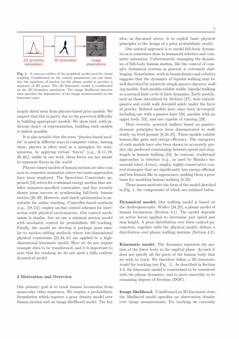
2D dynamics(simulation)
3D kinematics imageobservations
Fig. 1 A cartoon outline of the graphical model used for visualtracking. Conditioned on the control parameters one can simu-late the equations of motion for the planar model to produce asequence of 2D poses. The 3D kinematic model is conditionedon the 2D dynamics simulation. The image likelihood functionthen specifies the dependence of the image measurements on thekinematic pose.
largely shied away from physics-based prior models. We
suspect that this is partly due to the perceived difficulty
in building appropriate models. We show that, with ju-dicious choice of representation, building such models
is indeed possible.
It is also notable that the term “physics-based mod-
els” is used in different ways in computer vision. Amongthese, physics is often used as a metaphor for mini-
mization, by applying virtual “forces” (e.g., [6,11,19,
20,46]); unlike in our work, these forces are not meant
to represent forces in the world.
Physics-based models of human motion are also com-mon in computer animation where two main approaches
have been employed. The Spacetime Constraints ap-
proach [53] solves for a minimal-energy motion that sat-
isfies animator-specified constraints, and has recently
shown some success at synthesizing full-body humanmotion [26,39]. However, such batch optimization is un-
suitable for online tracking. Controller-based methods
(e.g., [18,55]) employ on-line control schemes for inter-
action with physical environments. Our control mech-anism is similar, but we use a minimal motion model
with stochastic control for probabilistic 3D tracking.
Finally, the model we develop is perhaps most simi-
lar to motion editing methods where low-dimensional
physical constraints [23,34,41] are applied to a high-dimensional kinematic model. Here we do not require
example data to be transformed, and it is important to
note that for tracking we do not need a fully-realistic
dynamical model.
3 Motivation and Overview
Our primary goal is to track human locomotion frommonocular video sequences. We employ a probabilistic
formulation which requires a prior density model over
human motion and an image likelihood model. The key
idea, as discussed above, is to exploit basic physical
principles in the design of a prior probabilistic model.
One natural approach is to model full-body dynam-ics as is sometimes done in humanoid robotics and com-
puter animation. Unfortunately, managing the dynam-
ics of full-body human motion, like the control of com-
plex dynamical systems in general, is extremely chal-
lenging. Nonetheless, work in biomechanics and roboticssuggests that the dynamics of bipedal walking may be
well described by relatively simple passive-dynamic walk-
ing models. Such models exhibit stable, bipedal walking
as a natural limit cycle of their dynamics. Early models,such as those introduced by McGeer [27], were entirely
passive and could walk downhill solely under the force
of gravity. Related models have since been developed,
including one with a passive knee [28], another with an
upper body [52], and one capable of running [29].
More recently, powered walkers based on passive-
dynamic principles have been demonstrated to walk
stably on level-ground [8,24,25]. These models exhibithuman-like gaits and energy-efficiency. The energetics
of such models have also been shown to accurately pre-
dict the preferred relationship between speed and step-
length in human walking [24]. In contrast, traditionalapproaches in robotics (e.g., as used by Honda’s hu-
manoid robot Asimo), employ highly-conservative con-
trol strategies that are significantly less energy-efficient
and less human-like in appearance, making them a poor
basis for modeling human walking [8,35].
These issues motivate the form of the model sketched
in Fig. 1, the components of which are outlined below.
Dynamical model. Our walking model is based on
the Anthropomorphic Walker [24,25], a planar model of
human locomotion (Section 4.1). The model depends
on active forces applied to determine gait speed andstep length. A prior distribution over these control pa-
rameters, together with the physical model, defines a
distribution over planar walking motions (Section 4.2).
Kinematic model. The dynamics represent the mo-
tion of the lower body in the sagittal plane. As such it
does not specify all the parts of the human body that
we wish to track. We therefore define a 3D kinematic
model for tracking (see Fig. 1). As described in Section4.3, the kinematic model is constrained to be consistent
with the planar dynamics, and to move smoothly in its
remaining degrees of freedom (DOF).
Image likelihood. Conditioned on 3D kinematic state,
the likelihood model specifies an observation density
over image measurements. For tracking we currently
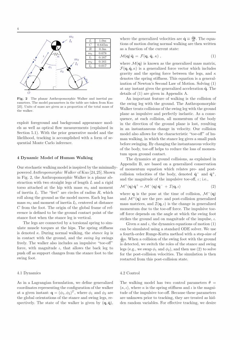
4
L 1.0m
C 0.645m
R 0.3m
mt 0.678
It 0.167
mℓ 0.161
Iℓ 0.017
Fig. 2 The planar Anthropomorphic Walker and inertial pa-rameters. The model parameters in the table are taken from Kuo[25]. Units of mass are given as a proportion of the total mass ofthe walker.
exploit foreground and background appearance mod-
els as well as optical flow measurements (explained inSection 5.1). With the prior generative model and the
likelihood, tracking is accomplished with a form of se-
quential Monte Carlo inference.
4 Dynamic Model of Human Walking
Our stochastic walking model is inspired by the minimally-
powered Anthropomorphic Walker of Kuo [24,25]. Shown
in Fig. 2, the Anthropomorphic Walker is a planar ab-
straction with two straight legs of length L and a rigid
torso attached at the hip with mass mt and momentof inertia It. The “feet” are circles of radius R, which
roll along the ground as the model moves. Each leg has
mass mℓ and moment of inertia Iℓ, centered at distance
C from the foot. The origin of the global frame of ref-erence is defined to be the ground contact point of the
stance foot when the stance leg is vertical.
The legs are connected by a torsional spring to sim-
ulate muscle torques at the hips. The spring stiffness
is denoted κ. During normal walking, the stance leg isin contact with the ground, and the swing leg swings
freely. The walker also includes an impulsive “toe-off”
force, with magnitude ι, that allows the back leg to
push off as support changes from the stance foot to theswing foot.
4.1 Dynamics
As in a Lagrangian formulation, we define generalized
coordinates representing the configuration of the walkerat a given instant: q = (φ1, φ2)
T , where φ1 and φ2 are
the global orientations of the stance and swing legs, re-
spectively. The state of the walker is given by (q, q),
where the generalized velocities are q ≡ dq
dt. The equa-
tions of motion during normal walking are then written
as a function of the current state:
M(q) q = F(q, q, κ) , (1)
where M(q) is known as the generalized mass matrix,
F(q, q, κ) is a generalized force vector which includesgravity and the spring force between the legs, and κ
denotes the spring stiffness. This equation is a general-
ization of Newton’s Second Law of Motion. Solving (1)
at any instant gives the generalized acceleration q. Thedetails of (1) are given in Appendix A.
An important feature of walking is the collision of
the swing leg with the ground. The Anthropomorphic
Walker treats collisions of the swing leg with the ground
plane as impulsive and perfectly inelastic. As a conse-quence, at each collision, all momentum of the body
in the direction of the ground plane is lost, resulting
in an instantaneous change in velocity. Our collision
model also allows for the characteristic “toe-off” of hu-man walking, in which the stance leg gives a small push
before swinging. By changing the instantaneous velocity
of the body, toe-off helps to reduce the loss of momen-
tum upon ground contact.
The dynamics at ground collisions, as explained inAppendix B, are based on a generalized conservation
of momentum equation which relates pre- and post-
collision velocities of the body, denoted q− and q+,
and the magnitude of the impulsive toe-off, ι ; i.e.,
M+(q) q+ = M−(q) q− + I(q, ι) (2)
where q is the pose at the time of collision, M−(q)and M+(q) are the pre- and post-collision generalized
mass matrices, and I(q, ι) is the change in generalized
momentum due to the toe-off force. The impulsive toe-
off force depends on the angle at which the swing footstrikes the ground and on magnitude of the impulse, ι.
Given κ and ι, the dynamics equations of motion (1)
can be simulated using a standard ODE solver. We use
a fourth-order Runge-Kutta method with a step-size of130 s. When a collision of the swing foot with the groundis detected, we switch the roles of the stance and swing
legs (e.g., we swap φ1 and φ2), and then use (2) to solve
for the post-collision velocities. The simulation is then
restarted from this post-collision state.
4.2 Control
The walking model has two control parameters θ =
(κ, ι), where κ is the spring stiffness and ι is the magni-tude of the impulsive toe-off. Because these parameters
are unknown prior to tracking, they are treated as hid-
den random variables. For effective tracking, we desire

5
0
0.5
1
0.811
1.22
0
5
10
0.811
1.22
Step length(m)
Step length(m)
Speed(m/s)
Speed(m/s)
Impulsemagnitude
Springstiffness
Fig. 3 Optimal stiffness κ (left) and impulse magnitude ι (right)as functions of speed and step length are shown. These plots il-lustrate the flexibility and expressiveness of the model’s controlparameters. Parameters were found by searching for cyclic mo-tions with the desired speed and step length.
a prior distribution over θ which, together with the dy-namical model, defines a distribution over motions. A
gait may then be generated by sampling θ and simulat-
ing the dynamics.
One might learn a prior over θ by fitting the An-thropomorphic Walker to human mocap data of people
walking with different styles, speeds, step-lengths, etc.
This is challenging, however, as it requires a significant
amount of mocap data, and the mapping from 3D kine-
matic description used for the mocap to the abstract 2Dplanar model is not obvious. Rather, we take a simpler
approach motivated by the principle that walking mo-
tions are characterized by stable, cyclic gaits. Our prior
over θ then assumes that likely control parameters liein the vicinity of those that produce cyclic gaits.
Determining cyclic gaits. The first step in the de-
sign of the prior is to determine the space of control
parameters that generate cyclic gaits spanning the nat-
ural range of human walking speeds and step-lengths.
This is readily formulated as an optimization problem.For a given speed and step-length, we seek initial condi-
tions (q0, q0) and parameters θ such that the simulated
motion ends in the starting state. The initial pose q0
can be directly specified since both feet must be onthe ground at the desired step-length. The simulation
duration T can determined by the desired speed and
step-length. We then use Newton’s method to solve
D(q0, q0, θ, T ) − (q0, q0) = 0 , (3)
for q0 and θ where D is a function that simulates the
dynamics for duration T given an initial state (q0, q0)and parameters θ. The necessary derivatives are com-
puted using finite differences. In practice, the solver was
able to obtain control parameters satisfying (3) up to
numerical precision for the tested range of speeds andstep-lengths.
Solving (3) for a discrete set of speeds and step-
lengths produces the control parameters shown in Fig-
0.40.6
-3
-2
-10
0.5
1
Swing leg pre-collisionangular velocity
(rad/s)
_Á¡¡
2
Impulse magnitude
_Á¡¡
1
Stance leg pre-collisionangular velocity
(rad/s)
Fig. 4 Impulse magnitude ι of the optimal cyclic gaits plottedversus pre-collision velocities q− = (φ−1 , φ
−
2 ). During tracking,a bilinear fit to the data shown here is used to determine theconditional mean for a Gamma density over ι at the beginning ofeach stride.
ure 3. These plots show optimal control parameters for
the full range of human walking speeds, ranging from 2
to 7 km/h, and for a wide range of step-lengths, roughly
0.5-1.2m. In particular, note that the optimal stiffness
and impulse magnitudes depend smoothly on the speedand step-length of the motion. This is important as it
indicates that the Anthropomorphic Walker is reason-
ably stable. To facilitate the duplication of our results,
we have published Matlab code which simulates themodel, along with solutions to (3), at http://www.cs.
toronto.edu/~mbrubake/permanent/awalker.
Stochastic control. To design a prior distribution over
walking motions for the Anthropomorphic Walker, weassume noisy control parameters that are expected to
lie in the vicinity of those that produce cyclic gaits.
We further assume that speed and step-length change
slowly from stride to stride. Walking motions are ob-
tained by sampling from the prior over the control pa-rameters and then performing deterministic simulation
using the equations of motion.
We assume that the magnitude of the impulsive toe-
off force, ι > 0, follows a Gamma distribution. For theoptimal cyclic gaits, the impulse magnitude was very
well fit by a bilinear function µι(q−) of the two pre-
collision velocities q− (see Fig. 4). This fit was per-
formed using least-squares regression with the solutions
to (3). The parameters of the Gamma distribution areset such that the mean is µι(q
−) and the variance is
0.052.
The unknown spring stiffness at time t, κt, is as-
sumed to be nearly constant throughout each stride,and to change slowly from one stride to the next. Ac-
cordingly, within a stride we define κt to be Gaussian
with constant mean κ and variance σ2κ:
κt ∼ N (κ, σ2κ) (4)
where N (µ, σ2) is a Gaussian distribution with mean
µ and variance σ2. Given the mean stiffness for the ith

6
Fig. 5 The 3D kinematic model is conditioned on the 2D planardynamics of the Anthropomorphic Walker.
stride, the mean stiffness for the next stride κ(i+1) is
given by
κ(i+1) ∼ N (βµκ + (1 − β)κ(i), σ2κ) (5)
where µκ is a global mean spring stiffness and β deter-mines how close κ(i) remains to µκ over time. We use
β = 0.85, σ2κ = 1.0, µκ = 0.7 and σ2
κ = 0.5.
During tracking, κ does not need to be explicitly
sampled. Instead, using a form of Rao-Blackwellization
[12,21], κ can be analytically marginalized out. Then,only the sufficient statistics of the resulting Gaussian
distribution over κ needs to be maintained for each par-
ticle.
Because the walking model is very stable, the model
is relatively robust to the choice of stochastic control.Other controllers may work just as well or better.
4.3 Conditional Kinematics
The model above is low-dimensional, easy to control,
and produces human-like gaits. Nevertheless, it is aplanar model, and hence it does not specify pose pa-
rameters in 3D. Nor does it specify all parameters of
interest, such as the torso, knees and feet. We therefore
add a higher-dimensional 3D kinematic model, condi-tioned on the underlying dynamics. The coupling of a
simple physics-based model with a detailed kinematic
model is similar to Popovic and Witkin’s physics-based
motion editing system [34].
The kinematic model, depicted in Fig. 5, has legs,
knees, feet and a torso. It has ball-and-socket joints atthe hips, a hinge joint for the knees and 2 DoF joints for
the ankles. Although the upper body is not used in the
physics model, it provides useful features for tracking.
The upper body in the kinematic model comprises asingle rigid body attached to the legs.
The kinematic model is constrained to match the
dynamics at every instant. In effect, the conditional
distribution of these kinematic parameters, given the
Joint Axis α* k ψ σ (ψmin, ψmax)
TorsoSide 0.9 5 0 25 (−∞,∞)Front 0.9 5 0 25 (−∞,∞)
Up 0.75 0 0 300 (−∞,∞)
HipFront 0.5 5 0 50 (−π
8, π
8)
Up 0.5 5 0 50 (−π8, π
8)
Stance Knee Side 0.75 20 0 50 (0, π)Swing Knee Side 0.9 15 ** 300 (0, π)
AnkleSide 0.9 50 0 50 (−π
8, π
8)
Front 0.9 50 0 50 (−π8, π
8)
Table 1 The parameters of the conditional kinematic modelused in tracking. The degrees of freedom not listed (Hip X) areconstrained to be equal to that of the Anthropomorphic Walker.(*) Values of α shown here are for ∆t = 1
30s. For ∆t = 1
60s, the
square roots of these values are used. (**) ψswing knee is handled
specially, see text for more details.
state of the dynamics, is a delta function. Specifically,
the upper-leg orientations of the kinematic model in
the sagittal plane are constrained to be equal to the
leg orientations in the dynamics. The ground contact
of stance foot in the kinematics and rounded “foot” ofthe dynamics are also forced to be consistent. In par-
ticular, the foot of the stance leg is constrained to be in
contact with the ground. The location of this contact
point on the foot rolls along the foot proportional to thearc-length with which the dynamics foot rolls forward
during the stride.
When the simulation of the Anthropomorphic Walkerpredicts a collision, the stance leg, and thus the contact
constraint, switches to the other foot. If the correspond-
ing foot of the kinematic model is far from the ground,
applying this constraint could cause a “jump” in the
pose of the kinematic model. However, such jumps aregenerally inconsistent with image data and are thus
not a significant concern. In general, this discontinuity
would be largest when the knee is very bent, which does
not happen in most normal walking. Because the An-thropomorphic Walker lacks knees, it is unable to han-
dle motions which rely on significant knee bend during
contact, such as running and walking on steep slopes.
We anticipate that using a physical model with moredegrees-of-freedom should address this issue.
Each remaining kinematic DOF ψj,t is modeled as
a smooth, 2nd-order Markov process:
ψj,t = ψj,t−1+∆tαjψj,t−1+∆t2(kj(ψj−ψj,t−1))+ηj)(6)
where ∆t is the size of the timestep, ψj,t−1 = (ψj,t−1 −ψj,t−2)/∆t is the joint angle velocity, and ηj is IID
Gaussian noise with mean zero and variance σ2j . This
model is analogous to a damped spring model withnoisy accelerations where kj is the spring constant, ψj is
the rest position, αj is related to the damping constant
and ηj is noisy acceleration. Joint limits which require
7
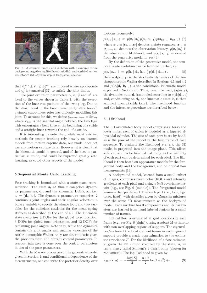
Fig. 6 A cropped image (left) is shown with a example of thebackground negative log likelihood (middle), and a grid of motiontrajectories (blue/yellow depict large/small speeds).
that ψminj ≤ ψj ≤ ψmax
j are imposed where appropriate
and ηj is truncated [37] to satisfy the joint limits.
The joint evolution parameters α, k, ψ and σ2 are
fixed to the values shown in Table 1, with the excep-
tion of the knee rest position of the swing leg. Due to
the sharp bend in the knee immediately after toe-off,a simple smoothness prior has difficulty modelling this
joint. To account for this, we define ψswing knee = 5ψhip
where ψhip is the sagittal angle between the two legs.
This encourages a bent knee at the beginning of a strideand a straight knee towards the end of a stride.
It is interesting to note that, while most existing
methods for people tracking rely heavily on learnedmodels from motion capture data, our model does not
use any motion capture data. However, it is clear that
the kinematic model in general, and of the knee in par-
ticular, is crude, and could be improved greatly with
learning, as could other aspects of the model.
5 Sequential Monte Carlo Tracking
Pose tracking is formulated with a state-space repre-
sentation. The state st at time t comprises dynam-
ics parameters, dt, and the kinematic DOFs, kt; i.e.,
st = (dt, kt). The dynamics parameters comprises 2continuous joint angles and their angular velocities, a
binary variable to specify the stance foot, and two vari-
ables for the sufficient statistics for the mean spring
stiffness as described at the end of 4.2. The kinematic
state comprises 3 DOFs for the global torso position,3 DOFs for global torso orientation, and 12 DOFs for
remaining joint angles. Note that, while the dynamics
contain the joint angles and angular velocities of the
Anthropomorphic Walker, they are deterministic giventhe previous state and current control parameters. In
essence, inference is done over the control parameters
in lieu of the pose parameters.
With the Markov properties of the generative model
given in Section 4, and conditional independence of the
measurements, one can write the posterior density over
motions recursively;
p(s1:t | z1:t) ∝ p(zt | st) p(st | st−1) p(s1:t−1 | z1:t−1) (7)
where s1:t ≡ [s1, ..., st] denotes a state sequence, z1:t ≡[z1, ..., zt] denotes the observation history, p(zt | st) is
the observation likelihood, and p(st | st−1) is derivedfrom the generative model in Sec. 4.
By the definition of the generative model, the tem-
poral state evolution can be factored further; i.e.,
p(st | st−1) = p(kt |dt, kt−1) p(dt |dt−1) . (8)
Here p(dt|dt−1) is the stochastic dynamics of the An-
thropomorphic Walker described in Sections 4.1 and 4.2
and p(kt|dt,kt−1) is the conditional kinematic model
explained in Section 4.3. Thus, to sample from p(st|st−1),
the dynamics state dt is sampled according to p(dt|dt−1)and, conditioning on dt, the kinematic state kt is then
sampled from p(kt|dt,kt−1). The likelihood function
and the inference procedure are described below.
5.1 Likelihood
The 3D articulated body model comprises a torso and
lower limbs, each of which is modeled as a tapered el-
lipsoidal cylinder. The size of each part is set by hand,
as is the pose of the model in the first frame of each
sequence. To evaluate the likelihood p(zt|st), the 3Dmodel is projected into the image plane. This allows
self-occlusion to be handled naturally as the visibility
of each part can be determined for each pixel. The like-
lihood is then based on appearance models for the fore-ground body and the background, and on optical flow
measurements [14].
A background model, learned from a small subset
of images, comprises mean color (RGB) and intensity
gradients at each pixel and a single 5×5 covariance ma-trix (e.g., see Fig. 6 (middle)). The foreground model
assumes that pixels are IID in each part (i.e., foot, legs,
torso, head), with densities given by Gaussian mixtures
over the same 5D measurements as the backgroundmodel. Each mixture has 3 components and its param-
eters are learned from hand labeled regions in a small
number of frames.
Optical flow is estimated at grid locations in each
frame (e.g., see Fig. 6 (right)), using a robust M-estimatorwith non-overlapping regions of support. The eigenval-
ues/vectors of the local gradient tensor in each region of
support provide a crude approximation to the estima-
tor covariance Σ. For the likelihood of a flow estimate,v, given the 2D motion specified by the state, u, we
use a heavy-tailed Student’s t distribution (chosen for
robustness). The log-likelihood is given by
log p(v|u) = −log |Σ|
2−n+2
2log(1+e2) + c (9)

8
where e2 = 12 (v − u)TΣ−1(v − u) and n = 2 is the
degrees of freedom, and c is a constant. Because the
camera is not moving in our image sequences, we de-
fine the log-likelihood of a flow measurement on the
background as given by (9) with u = 0.
The visibility of each part defines a partition of
the observations, such that zt(i) are the measurementswhich belong to part i. The background is simply treated
as another part. Then the log-likelihood contribution of
part i is
log p(zt(i)|st) =∑
m∈zt(i)
log p(m|st) (10)
where the sum is over the measurements belonging topart i. To cope with large correlations between mea-
surement errors, we define the appearance and flow log-
likelihood to be the weighted sum of log-likelihoods over
all visible measurements for each part
log p(zt|st) =∑
i
wi log p(zt(i)|st) (11)
where the weights are set inversely proportional to theexpected size of each part in the image.1 If multiple
cameras are available, they are assumed to be condi-
tionally independent given the state st. This yields a
combined log-likelihood of
log p(z1t , z
2t , · · · | st) =
∑
i
log p(zit | st) (12)
where zit is the observation from camera i.
5.2 Inference
Using a particle filter, we approximate the posterior
(7) by a weighted set of N samples St ={s(j)1:t , w
(j)t }N
j=1.Given the recursive form of (7), the posterior St, given
St−1, can be computed in two steps; i.e.,
1. Draw samples s(j)t ∼ p(st | s
(j)t−1) using (8) to form
the new state sequences s(j)1:t = [s
(j)1:t−1, s
(j)t ]; and
2. Update the weights w(j)t = cw
(j)t−1 p(zt | s
(j)t ) , where
c is used to normalize the weights so they sum to 1.
This approach, without re-sampling, often works welluntil particle depletion becomes a problem, i.e., where
only a small number of weights are significantly non-
zero. One common solution to this is to re-sample the
states in St according to their weights. This is well-known to be suboptimal since it does not exploit the
current observation in determining which states should
1 To avoid computing the log-likelihood over the entire image,we equivalently compute log-likelihood ratios of foreground ver-sus background over regions of the image to which the 3D bodygeometry projects.
be re-sampled (i.e., survive). Instead, inspired by the
auxiliary particle filter [33], we use future data to pre-
dict how well current samples are likely to fare in the
future. This is of particular importance with a physics-
based model, where the quality of a sample is not al-ways immediately evident based on current and past
likelihoods. For instance, the consequences of forces ap-
plied at the current time may not manifest until several
frames into the future.In more detail, we maintain an approximation St:t+τ =
{s(j)t:t+τ , w
(j)t:t+τ}
Nj=1 to the marginal posterior distribu-
tion over state sequences in a small temporal windowof τ + 1 frames, p(st:t+τ | z1:t+τ ). The sample set is ob-
tained by simulating the model for τ + 1 time steps,
given St−1, evaluating the likelihood of each trajectory
and setting
w(j)t:t+τ = cw
(j)t−1
t+τ∏
ℓ=t
p(zℓ|s(j)ℓ ) (13)
where c is set such that the weights sum to one.
Following [12,22], when the effective number of sam-
ples,
Neff =
∑
j
(w(j)t:t+τ )2
−1
, (14)
becomes too small we re-sample St−1 using importancesampling; i.e.,
1. Draw samples s(k)t−1 from the weights {w
(j)t−1}
Nj=1 where
w(j)t−1 = (1 − γ)w
(j)t−1 + γw
(j)t:t+τ and γ represents our
trust in our approximation St:t+τ ;
2. Set the new weights to be w(k)t−1/w
(k)t−1, and then nor-
malize the weights so they sum to 1.
The importance re-weighting (step 2) is needed to main-tain a properly weighted approximation to the posterior
(7). Below we use τ =3 and γ=0.9. With this form of
importance sampling, resampling occurs once every 4
or 5 frames on average for the experiments below.
6 Results
Here we present the results of four experiments with
our model. The first three experiments use the same
set of parameters for the kinematic evolution and the
same prior over the control parameters for the dynam-ics. The parameters for the fourth experiment were set
to similar values, but adjusted to account for a differ-
ence in frame rate (30 frames per second for experi-
ments one through three and 60 frames per second forexperiment four). These parameters were empirically
determined. Finally, for each image sequence, we deter-
mine the camera intrinsics and extrinsics with respect

9
Fig. 7 Composite images show the subject at several frames, depicting the motion over the 130 frame sequence: (left) the original im-ages; (middle) the inferred poses of the MAP kinematics overlayed on the images, with the corresponding state of the AnthropomorphicWalker depicted along the bottom (the stance leg in red); (right) a 3D rendering of MAP poses from a different viewpoint.
Fig. 9 Two rows of cropped images showing every second frame of the MAP trajectory in Experiment 1 for two strides during changeof speed: (top) the kinematic skeleton is overlayed on the subject; (middle) the corresponding state of the Anthropomorphic Walkeris shown with the stance printed in red; (bottom) a 3D rendering of the kinematic state.
to a world coordinate frame on the ground plane based
on 10-12 correspondences between image locations and
ground truth 3D locations in each scene. The direction
of gravity is assumed to be normal to the ground plane.
All experiments used 5000 particles, with resam-
pling when Neff < 500. Experimentally we have found
that, while as few as 1000 particles can result in suc-
cessful tracking of some sequences (e.g., experiment 1),
5000 particles was necessary to consistently track well
across all experiments. Excluding likelihood computa-
tions, the tracker runs at around 30 frames per sec-ond. The body geometry was set by hand and the mean
initial state was coarsely hand-determined. Initial par-
ticles were sampled with a large variance about that

10
Fig. 10 Composite images show the input data (left), background model (middle) and MAP trajectory (right) at several frames forExperiment 2. Only the outline of the occluder is shown for illustration.
Fig. 11 Cropped images showing every 4th frame of the MAP trajectory (top), the corresponding state of the Anthropomorphicwalker (middle) and the posterior distribution (bottom) in Experiment 2. In the posterior points on the head (blue), left and rightfeet (white and yellow), left and right knees (green and red) and hip (blue) are plotted for each particle with intensity proportional totheir log weight.
0 20 40 60 80 100 120 1402
3
4
5
6
7
Vel
ocity
(km
/h)
0 20 40 60 80 100 120 1400
0.5
1
P(St
ance
Leg
= L
eft)
Fig. 8 Inferred speed as a function of time for the MAPtrajectory in Experiment 1 (blue). The dashed green line isp(stance leg = left|z1:t), the probability of the left leg being thestance leg given the data up to that frame.
mean state. The inference procedure results in a set
of particles that approximate the posterior distribution
p(s1:t | z1:t) for a given time t. Our demonstration of the
results will focus mainly on the maximum a-posteriori
(MAP) trajectory of states over all T frames,
sMAP1:T = arg max
s1:Tp(s1:T | z1:T ) . (15)
This is crudely approximated by choosing the state se-
quence associated with the particle at time T with thelargest weight. We present the MAP trajectory because
it ensures that the sequence of poses is consistent with
the underlying motion model.
Experiment 1: Changes in Speed. Figure 7 (left)
shows a composite image of a walking sequence in which
the subject’s speed decreases from almost 7 to 3 km/h.
Figure 8 shows the recovered velocity of the subjectover time in the solid blue curve. Also shown with the
dashed green curve is the posterior probability of which
leg is the stance leg. Such speed changes are handled
naturally by the physics-based model. Fig. 7 (middle)shows the recovered MAP trajectory from the original
camera position while Fig. 7 (right) shows that the re-
covered motion looks good in 3D from other views.

11
Fig. 12 3D rendering of the MAP trajectory in Experiment 2.
Figure 9 shows cropped versions of tracking resultsfor a short subsequence, demonstrating the consistency
of the tracker. Weakness in the conditional kinematic
model at high speeds leads to subtle anomolies, espe-
cially around the knees, which can be seen in the early
frames of this subsequence.
Experiment 2: Occlusion. We simulate occlusion by
blacking out an image region as shown in Figure 10. Thesilhouette of the lower body is therefore lost, and we
discard all flow measurements that encroach upon the
occluder. Nevertheless, the subtle motion of the torso
is enough to track the person, infer foot positions, andrecover 3D pose.
It is particularly interesting to examine the poste-
rior distribution p(st|z1:t) which can be seen in the bot-
tom row of Figure 11. These images show colour coded
points for the head, hip, knees and feet for each particle
in the posterior. The brightness of each point is propor-tional to its log weight. While there is increased poste-
rior uncertainty during the occlusion, it does not diffuse
monotonically. Rather, motion of the upper body allows
the tracker to infer the stance leg and contact location.Notice that, soon after ground contacts, the marginal
posterior over the stance foot position tends to shrink.
Finally, during occlusion, leg-switching can occur
but is unlikely. This is visible in the posterior distribu-
tion as an overlap between yellow (right foot) and white
(left foot) points. However, the ambiguity is quickly re-solved after the occlusion.
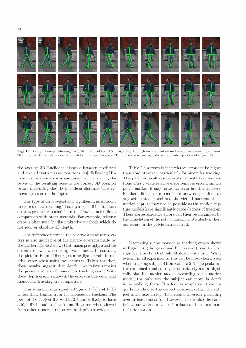
Experiment 3: Turning. While the Anthropomor-phic Walker is a planar model we are still able to suc-
cessfully track 3D walking motions because of the con-
ditional kinematics. As can been seen in Figure 14, the
model successfully tracks the person through a sharpturn in a sequence of more than 400 frames. Despite
the limitations of the physical model, it is able to accu-
rately represent the dynamics of the motion in 2D while
200 250 300 350
2
3
4
5
6
Vel
oci
ty (
km
/h)
200 250 300 3500
0.5
1
P(S
tan
ce L
eg =
Lef
t)
Fig. 13 MAP trajectory velocity (blue) and stance leg posteriorp(stance leg = left|z1:t) (dashed green) for the times shown inFigure 14. The highlighted region, corresponding to the middlerow of Figure 14, exhibits significant uncertainty about which legis the stance leg.
the conditional kinematic model represents the turning
motion.
Figure 13 shows the speed of the subject and the
posterior probability of which leg is the stance leg. Be-
tween frames 250 and 300 there is significant uncer-tainty in which leg is in contact with the ground. This
is partly because, in these frames which correspond to
the middle row in Figure 14, there are few visual cues
to disambiguate when a foot has hit the ground.
Experiment 4: HumanEva. To quantitatively assess
the quality of tracking, we also report results on the Hu-
manEva benchmark dataset [43]. This dataset contains
multicamera video, synchronized with motion capture
data that can be used as ground truth. Error is mea-sured as the average Euclidean distance over a set of
defined marker positions. Because our method does not
actively track the head and arms, we report results us-
ing only the markers on the torso and legs.
As above, tracking was hand initialized and segmentlengths were set based on the static motion capture
available for each subject. The camera calibration pro-
vided with the dataset was used and it was assumed
that the ground plane was located at Z = 0. We reportmonocular and binocular results on subjects 2 and 4
from HumanEva II. Error is measured from the poses
in the MAP trajectory of states over all T frames. The
results are summarized in Table 2 and errors over time
are plotted in Figures 15 and 16.It is important to note that the same model (dynam-
ics and kinematics) is used to track the two HumanEva
subjects as well as the subject in the preceeding exper-
iments. Only the body size parameters were different.
This helps to demonstrate that the model can general-ize to different subjects.
In this paper, both relative and absolute 3D error
measures are reported. Absolute error is computed as
12
Fig. 14 Cropped images showing every 5th frame of the MAP trajectory through an acceleration and sharp turn, starting at frame200. The skeleton of the kinematic model is overlayed in green. The middle row corresponds to the shaded portion of Figure 13.
the average 3D Euclidean distance between predicted
and ground truth marker positions [43]. Following Hu-
manEva, relative error is computed by translating the
pelvis of the resulting pose to the correct 3D position
before measuring the 3D Euclidean distance. This re-moves gross errors in depth.
The type of error reported is significant, as different
measures make meaningful comparisons difficult. Both
error types are reported here to allow a more direct
comparison with other methods. For example, relativeerror is often used by discriminative methods which do
not recover absolute 3D depth.
The difference between the relative and absolute er-
rors is also indicative of the nature of errors made by
the tracker. Table 2 shows that, unsurprisingly, absoluteerrors are lower when using two cameras. In contrast,
the plots in Figure 16 suggest a negligable gain in rel-
ative error when using two cameras. Taken together,
these results suggest that depth uncertainty remainsthe primary source of monocular tracking error. With
these depth errors removed, the errors in binocular and
monocular tracking are comparable.
This is further illustrated in Figures 17(a) and 17(b)
which show frames from the monocular trackers. Thepose of the subject fits well in 2D and is likely to have
a high likelihood at that frame. However, when viewed
from other cameras, the errors in depth are evident.
Table 2 also reveals that relative error can be higher
than absolute error, particularly for binocular tracking.
This peculiar result can be explained with two observa-
tions. First, while relative error removes error from the
pelvic marker, it may introduce error in other markers.Further, direct correspondences between positions on
any articulated model and the virtual markers of the
motion capture may not be possible as the motion cap-
ture models have significantly more degrees of freedom.These correspondence errors can then be magnified by
the translation of the pelvic marker, particularly if there
are errors in the pelvic marker itself.
Interestingly, the monocular tracking errors shown
in Figure 15 (the green and blue curves) tend to havesignificant peaks which fall off slowly with time. While
evident in all experiments, this can be most clearly seen
when tracking subject 4 from camera 2. These peaks are
the combined result of depth uncertainty and a physi-
cally plausible motion model. According to the motionmodel, the only way the subject can move in depth
is by walking there. If a foot is misplaced it cannot
gradually slide to the correct position, rather the sub-
ject must take a step. This results in errors persistingover at least one stride. However, this is also the same
behaviour which prevents footskate and ensures more
realistic motions.

13
Sequence Error TypeMonocular (Camera 2) Monocular (Camera 3) Binocular (Cameras 2 and 3)Median Mean Median Mean Median Mean
Subject 2, Combo 1, Frames 25-350Absolute 82mm 88mm ± 38 67mm 82mm ± 34 52mm 53mm ± 9
Relative 67mm 70mm ± 13 67mm 67mm ± 11 64mm 66mm ± 9
Subject 4, Combo 4, Frames 15-350*Absolute 98mm 127mm ± 70 77mm 96mm ± 42 52mm 54mm ± 10Relative 74mm 76mm ± 17 71mm 70mm ± 10 65mm 66mm ± 10
Table 2 Quantitative results on sequences from HumanEva II. (*) As noted on the HumanEva II website, frames 298-335 are excludedfrom the calculation due to errors in the ground truth motion capture data.
0 50 100 150 200 250 300 3500
50
100
150
200
250
300
350
Frame Number
Abs
olut
e M
arke
r E
rror
(m
m)
0 50 100 150 200 250 300 3500
50
100
150
200
250
300
350
Frame Number
Abs
olut
e M
arke
r E
rror
(m
m)
Fig. 15 Average absolute marker error over time for Subject 2, Combo 1 (left) and Subject 4, Combo 4 (right). Plots are shownfor monocular tracking with camera 2 (solid blue) and camera 3 (dashed green) as well as binocular tracking with cameras 2 and 3(dot-dashed red).
0 50 100 150 200 250 300 3500
50
100
150
200
250
300
350
Frame Number
Rel
ativ
e M
arke
r E
rror
(m
m)
0 50 100 150 200 250 300 3500
50
100
150
200
250
300
350
Frame Number
Rel
ativ
e M
arke
r E
rror
(m
m)
Fig. 16 Average relative marker error over time for Subject 2, Combo 1 (left) and Subject 4, Combo 4 (right). Plots are shownfor monocular tracking with camera 2 (solid blue) and camera 3 (dashed green) as well as binocular tracking with cameras 2 and 3(dot-dashed red).
(a) Subject 2, Combo 1, Camera 3. The pose at frame 225 ofthe MAP trajectory is shown from camera 3 on the left. Onthe right are the views from cameras 2 and 4 respectively.
(b) Subject 4, Combo 4, Camera 2. The pose at frame 125 ofthe MAP trajectory is shown from camera 2 on the left. Onthe right are the views from cameras 3 and 4 respectively.
Fig. 17 Monocular tracking errors due to depth ambiguities. In both examples, the model appears to fit well in the view from whichtracking is done. However, when viewed from other cameras the errors in depth become evident.

14
7 Discussion and Future Work
In this paper we showed that physics-based models of-
fer significant benefits in terms of accuracy, stability,
and generality for person tracking. Results on three dif-ferent subjects in a variety of conditions, including in
the presence of severe occlusion, are presented which
demonstrate the ability of the tracker to generalize.
Quantitative results for monocular and binocular 3Dtracking on the HumanEva dataset [43] allows for di-
rect comparison with other methods.
Here we used a simple powered walking model, but
we are currently exploring more sophisticated physical
models [4] which may yield even more general trackers
for other types of motion. There will, generally, be a
trade-off between model generality and the difficulty ofdesigning a controller [50]. We note that, while control
of humanoid dynamical models is a challenging prob-
lem, there is a substantial literature in robotics and
animation from which to draw inspiration.
Although our approach employs online Bayesian in-
ference, it should also be possible to incorporate phys-ical laws within other tracking frameworks such as dis-
criminative methods. Models similar to this may also
be used for modelling and tracking other animals [15].
Acknowledgements Thanks to Zoran Popovic and Allan Jep-son for valuable discussions. Thanks to Jack Wang for some initialsoftware.
References
1. A. Agarwal and B. Triggs. Recoving 3D Human Pose fromMonocular Images. IEEE PAMI, 28(1):44–58, 2006.
2. A. Bissacco. Modeling and Learning Contact Dynamics inHuman Motion. In Proceedings of IEEE CVPR, volume 1,pages 421–428, 2005.
3. R. Blickhan and R. J. Full. Similarity in multilegged loco-motion: Bouncing like a monopode. Journal of Comparative
Physiology A: Neuroethology, Sensory, Neural, and Behav-
ioral Physiology, 173(5):509–517, Nov. 1993.4. M. A. Brubaker and D. J. Fleet. The Kneed Walker for
human pose tracking. In Proceedings of IEEE CVPR, 2008.5. M. A. Brubaker, D. J. Fleet, and A. Hertzmann. Physics-
based person tracking using simplified lower-body dynamics.In Proceedings of IEEE CVPR, 2007.
6. M. Chan, D. Metaxas, and S. Dickinson. Physics-BasedTracking of 3D Objects in 2D Image Sequences. In Pro-
ceedings of ICPR, pages 432–436, 1994.7. K. Choo and D. J. Fleet. People tracking using hybrid Monte
Carlo filtering. In Proceedings of IEEE ICCV, volume II,pages 321–328, 2001.
8. S. Collins, A. Ruina, R. Tedrake, and M. Wisse. EfficientBipedal Robots Based on Passive-Dynamic Walkers. Science,307(5712):1082–1085, 2005.
9. S. H. Collins and A. Ruina. A Bipedal Walking Robot withEfficient and Human-Like Gait. In Proceedings of IEEE Con-
ference on Robotics and Automation, 2005.
10. S. H. Collins, M. Wisse, and A. Ruina. A Three-DimensionalPassive-Dynamic Walking Robot with Two Legs and Knees.International Jounral of Robotics Research, 20(7):607–615,
2001.11. Q. Delamarre and O. Faugeras. 3D articulated models and
multiview tracking with physical forces. CVIU, 81(3):328–357, 2001.
12. A. Doucet, S. Godsill, and C. Andrieu. On sequential MonteCarlo sampling methods for Bayesian filtering. Statistics and
Computing, 10(3):197–208, 2000.13. A. Elgammal and C.-S. Lee. Inferring 3D body pose from
silhouettes using activity manifold learning. In Proceedings
of IEEE CVPR, volume 2, pages 681–688, 2004.14. D. Fleet and Y. Weiss. Optical flow estimation. In Math-
ematical Models of Computer Vision: The Handbook, pages239–258. Springer, 2005.
15. R. J. Full and D. E. Koditschek. Templates and An-chors: Neuromechanical Hypotheses of Legged Locomotionon Land. Journal of Experimental Biology, 202:3325–3332,1999.
16. H. Goldstein, C. P. Poole, and J. L. Safko. Classical Me-
chanics. Addison Wesley, 3rd edition, 2001.17. L. Herda, R. Urtasun, and P. Fua. Hierarchical implicit sur-
face joint limits for human body tracking. CVIU, 99(2):189–209, 2005.
18. J. K. Hodgins, W. L. Wooten, D. C. Brogan, and J. F.O’Brien. Animating human athletics. In Proceedings of SIG-
GRAPH, pages 71–78, 1995.19. L. Kakadiaris and D. Metaxas. Model-based estimation of
3D human motion. IEEE PAMI, 22(12):1453–1459, 2000.20. M. Kass, A. Witkin, and D. Terzopoulos. Snakes: Active
contour models. IJCV, 1(4):321–331, 1987.21. Z. Khan, T. Balch, and F. Dellaert. A rao-blackwellized par-
ticle filter for eigentracking. In Proceedings of IEEE CVPR,volume 2, pages 980–986, 2004.
22. A. Kong, J. S. Liu, and W. H. Wong. Sequential imputa-tions and bayesian missing data problems. Journal of the
American Statistical Association, 89(425):278–288, 1994.23. L. Kovar, J. Schreiner, and M. Gleicher. Footskate Cleanup
for Motion Capture Editing. In Proceedings of Symposium
on Computer Animation, 2002.24. A. D. Kuo. A Simple Model of Bipedal Walking Predicts
the Preferred Speed–Step Length Relationship. Journal of
Biomechanical Engineering, 123(3):264–269, 2001.25. A. D. Kuo. Energetics of Actively Powered Locomotion Us-
ing the Simplest Walking Model. Journal of Biomechanical
Engineering, 124(1):113–120, 2002.26. C. K. Liu, A. Hertzmann, and Z. Popovic. Learning physics-
based motion style with nonlinear inverse optimization. ACM
Transactions on Graphics, 24(3):1071–1081, 2005.27. T. McGeer. Passive Dynamic Walking. International Journal
of Robotics Research, 9(2):62–82, 1990.28. T. McGeer. Passive Walking with Knees. In Proceedings
of International Conference on Robotics and Automation,volume 3, pages 1640–1645, 1990.
29. T. McGeer. Principles of Walking and Running. In Advances
in Comparative and Environmental Physiology, volume 11,chapter 4, pages 113–139. Springer-Verlag, 1992.
30. D. Metaxas and D. Terzopoulos. Shape and nonrigid motionestimation through physics-based synthesis. IEEE PAMI,15(6):580–591, 1993.
31. V. Pavlovic, J. Rehg, T.-J. Cham, and K. Murphy. A dy-
namic Bayesian network approach to figure tracking usinglearned dynamic models. In Proceedings of IEEE ICCV,pages 94–101, 1999.
32. A. Pentland and B. Horowitz. Recovery of Nonrigid Motionand Structure. IEEE PAMI, 13(7):730–742, 1991.
33. M. K. Pitt and N. Shepard. Filtering via simulation: Auxilaryparticle filters. Journal of the American Statistical Associa-
tion, 94:590–599, 1999.

15
34. Z. Popovic and A. Witkin. Physically based motion transfor-mation. In Proceedings of SIGGRAPH, pages 11–20, 1999.
35. G. A. Pratt. Legged robots at MIT: what’s new since Raib-ert? IEEE Robotics & Automation, 7(3):15–19, 2000.
36. A. Rahimi, B. Recht, and T. Darrell. Learning AppearanceManifolds from Video. In Proceedings of IEEE CVPR, pages868–875, 2005.
37. C. P. Robert. Simulation of truncated normal variables.Statistics and Computing, 5(2):121–125, 1995.
38. R. Rosales, V. Athitsos, L. Sigal, and S. Sclaroff. 3D handpose reconstruction using specialized mappings. In Proceed-
ings of IEEE ICCV, volume 1, pages 378–385, 2001.39. A. Safonova, J. K. Hodgins, and N. S. Pollard. Synthesiz-
ing physically realistic human motion in low-dimensional,behavior-specific spaces. ACM Transactions on Graphics,23(3):514–521, 2004.
40. G. Shakhnarovich, P. Viola, and T. Darrell. Fast pose esti-mation with parameter-sensitive hashing. In Proceedings of
IEEE ICCV, pages 750–757, 2003.41. H. J. Shin, L. Kovar, and M. Gleicher. Physical Touchup of
Human Motions. In Proceedings of Pacific Graphics, pages194–203, 2003.
42. H. Sidenbladh, M. J. Black, and D. J. Fleet. StochasticTracking of 3D Human Figures Using 2D Image Motion. InProceedings of IEEE ECCV, volume 2, pages 702–718, 2000.
43. L. Sigal and M. Black. HumanEva: Synchronized videoand motion capture dataset for evaluation of articulated hu-man motion. Technical Report CS-06-08, Computer Science,Brown University, 2006.
44. C. Sminchisescu and A. Jepson. Generative modeling forcontinuous non-linearly embedded visual inference. In Pro-
ceedings of ICML, pages 96–103, 2004.45. C. Sminchisescu, A. Kanaujia, and D. Metaxas. BME3: Dis-
criminative density propagation for visual tracking. IEEE
PAMI, 29(11):2030–2044, 2007.46. D. Terzopoulos and D. Metaxas. Dynamic 3D models with
local and global deformations: deformable superquadrics. InProceedings of IEEE ICCV, pages 606–615, 1990.
47. R. Urtasun, D. J. Fleet, and P. Fua. 3D People Trackingwith Gaussian Process Dynamical Models. In Proceedings of
IEEE CVPR, volume 1, pages 238–245, 2006.48. R. Urtasun, D. J. Fleet, A. Hertzmann, and P. Fua. Priors
for People Tracking from Small Training Sets. In Proceedings
of IEEE ICCV, volume 1, pages 403–410, 2005.49. R. Q. van der Linde and A. L. Schwab. Lecture Notes Multi-
body Dynamics B, wb1413, course 1997/1998. Lab. for En-gineering Mechanics, Delft Univ. of Technology, 2002.
50. M. Vondrak, L. Sigal, and O. C. Jenkins. Physical simulation
for probabilistic motion tracking. In Proceedings of IEEE
CVPR, 2008.51. S. Wachter and H. H. Nagel. Tracking Persons in Monocular
Image Sequences. CVIU, 74(3):174–192, June 1999.52. M. Wisse, D. G. E. Hobbelen, and A. L. Schwab. Adding an
upper body to passive dynamic walking robots by means ofa bisecting hip mechanism. IEEE Transactions on Robotics,23(1):112–123, 2007.
53. A. Witkin and M. Kass. Spacetime Constraints. In Proceed-
ings of SIGGRAPH, volume 22, pages 159–168, 1988.54. C. R. Wren and A. Pentland. Dynamics models of human mo-
tion. In Proceecings of Automatic Face and Gesture Recog-
nition, 1998.55. K. Yin, K. Loken, and M. van de Panne. SIMBICON: Simple
biped locomotion control. ACM Transactions on Graphics,26(3), 2007.
A Equations of motion
Here we describe the equations of motion for the Anthropomor-
phic Walker, shown in Fig. 2. While general-purpose physics en-
gines may be used to implement the physical model and theimpulsive collisions with the ground, most do not support ex-act ground constraints, but instead effectively require the use
of springs to model static contact. In our experience it is notpossible to make the springs stiff enough to accurately model thedata without resulting in slow or unstable simulations. Hence, wederive equations of motion which exactly enforce static contactconstraints. These equations produces stable simulations whichallow (3) to be solved efficiently.
In order to derive the equations of motion for the walkingmodel, we employ the TMT method [49], a convenient recipefor constrained dynamics. The TMT formulation is equivalent toLagrange’s equations of motion and can be derived in a similarway, using d’Alembert’s Principle of virtual work [16]. However,we find the derivation of equations of motion using the TMTmethod simpler and more intuitive for articulated bodies.
We begin by defining the kinematic transformation, whichmaps from the generalized coordinates q = (φ1, φ2) to a 6 × 1vector that contains the linear and angular coordinates of eachrigid body which specify state for the Newton-Euler equationsof motion. The torso is treated as being rigidly connected to thestance leg and hence we have only two rigid parts in the An-thropomorphic Walker. The kinematic transformation can thenbe written as
k(q) =
−Rφ1 − (C1 − R) sinφ1
R+ (C1 −R) cosφ1
φ1
−Rφ1 − (L− R) sinφ1 + (L− C) sinφ2
R+ (L−R) cosφ1 − (L− C) cosφ2
φ2
(16)
where C1 =(Cmℓ+Lmt)
mℓ+mtis the location along the stance leg of
the combined center rigid body. Dependence of angles on timeis omitted for brevity. The origin, O, of the coordinate system ison the ground as shown in Fig. 2. The origin is positioned suchthat, when the stance leg is vertical, the bottom of the stanceleg and the origin are coincident. Assuming infinite friction, thecontact point between the rounded foot and the ground moves asthe stance leg rotates.
The equations of motion are summarized as
TT MTq = f + TT M (a − g) (17)
where the matrix T is the 6×2 Jacobian of k, i.e., T = ∂k/∂q.The reduced mass matrix is
M = diag(m1,m1, I1,mℓ,mℓ, Iℓ) , (18)
where m1 = mℓ +mt is the combined mass of the stance leg. Thecombined moment of inertia of the stance leg is given by
I1 = Iℓ + It + (C1 − C)2mℓ + (L− C1)2mt (19)
The convective acceleration is
g =∂
∂q
(
∂k
)
q (20)
and a = g[0,−1, 0, 0,−1, 0]T is the generalized acceleration vectordue to gravity (g = 9.8m/s2). The generalized spring force isf = κ[φ2 − φ1, φ1 − φ2]T . By substitution of variables, it can beseen that (17) is equivalent to (1), with M(q) = TT MT andF(q, q, κ) = f + TT M (a − g).
B Collision and support transfer
Since the end of the swing leg is even with the ground whenφ1 = −φ2, collisions are found by detecting zero-crossings of

16
C(φ1, φ2) = φ1 + φ2. However, our model also allows the swingfoot to move below the ground2, and thus a zero-crossing canoccur when the foot passes above the ground. Hence, we detect
collisions by detecting zero-crossings of C when φ1 < 0 and C < 0.The dynamical consequence of collision is determined by a
system of equations relating the instantaneous velocities imme-diately before and after the collision. By assuming ground colli-sions to be impulsive and inelastic the result can be determinedby solving a set of equations for the post-collision velocity. Tomodel toe-off before such a collision, an impulse along the stanceleg is added. In particular, the post-collision velocities q+ can besolved for using
T+T MT+q+ = T+T (v + MTq−) (21)
where q− are the pre-collision velocities, T is the pre-collisionkinematic transfer matrix specified above,
k+(q−) =
−Rφ2 −(L−R) sinφ2 + (L−C) sinφ1
R + (L−R) cosφ2 − (L−C) cosφ1
φ1
−Rφ2 − (C1−R) sinφ2
R+ (C1−R) cos φ2
φ2
(22)
is the post-collision kinematic transformation function, T+ =∂k+/∂q, is the post-collision kinematic transfer matrix, M isthe mass matrix as above and
v = ι[− sinφ1, cosφ1, 0, 0, 0, 0]T (23)
is the impulse vector with magnitude ι. Defining
M+(q) = T+TMT+T (24)
M−(q) = T+TMT (25)
I(q, ι) = T+Tv (26)
and substituting into (21) gives (2).At collision, the origin of the coordinate system shifts forward
by 2(Rφ2 +(L−R) sinφ2). The swing and stance leg switch roles;i.e., φ1 and φ2 and their velocities are swapped. Simulation thencontinues as before.
2 Because the Anthropomorphic Walker does not have knees,it can walk only by passing a foot through the ground.