Physics 361Principles of Modern Physics

Lecture 11

Bound States using the Schrödinger Equation

This lecture• More of solving problems with the Schrödinger

equation• Boundary conditions• Normalization and bound states

Next lectures• Particle in an infinite box potential• Solving more problems with the Schrödinger equation

Exponential solutions

When the total energy is less than the potential we have exponential solutions

If we have the potential starting at position x=0we would need an exponentially decreasing solutionsince we cannot have an infinite probabilityfor having a particle located in that region.Such effects can cause bound states to occur.

o

V

E

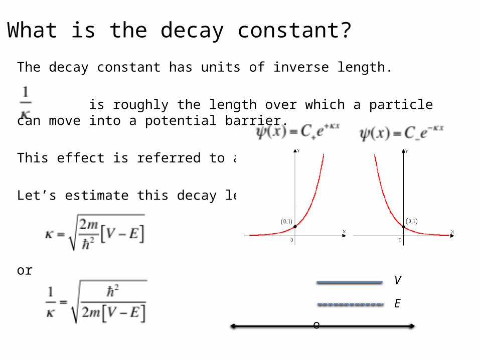
What is the decay constant?

The decay constant has units of inverse length.

is roughly the length over which a particle can move into a potential barrier.

This effect is referred to as tunneling.

Let’s estimate this decay length

or

o

V

E

What is the decay constant for an electron?

We need a relevant energy scale – ie, the potential barrier.Remember when we used looked into photoelectric effect, we knocked electrons out of matter with a couple eV photons. So let’s take the energy barrier to be an eV=1.6x10-19J. We have

which gives

Notice that this is a very short distance!For larger masses, it is even smaller, so larger masses seem to classically bounceoff barriers. o

V

E

Energy eigenstates

We have now found two classes of solutions to the Schrödinger equation, exponential and periodic (or sinusoidal).

We will generally be interested in energy-conserving solutions of the Schrödinger Eq. So we will solve thetime-independent form.

To do this, we will generally have anarbitrary potential, so we will need to solvefor for a specific . We have introduced the subscript E to it is a constant energy solutions – aka an “energy eigenstate”.

Boundary conditions

To have bound states requires some sort of bounds. To determine the effects of the boundaries, we need to know some boundary conditions (constraints).

V

E

Boundary conditions according to Schrödinger Eq.

Let’s first consider a single general boundary

We can integrate from any two points to obtain the first derivative of the wave function

V

E

Boundary conditions according to Schrödinger Eq. -2

As we integrate across the boundary, we add up the area under the curve between bounds.

We can integrate from any two points to obtain the first derivative of the wave function

V

E

Boundary conditions according to Schrödinger Eq. -3

How can change as we go across some abrupt potential change?

For a finite jump in potential the area to the right of the jump must approach zero as .Thus, the first derivative of the wave function is continuous for finite abrupt changes in potential. We can only have a finite discontinuity in the first derivative of the wave function for an infinite potential jump.

V

E

Boundary conditions according to Schrödinger Eq. -4

We can employ the same arguments again to determine that is continuous regardless of the potential jump.

Two boundary conditions for finite potential jumps.Continuity of both and

Two boundary conditions for infinite potential jumps.Continuity of , but a finite discontinuity of

V

E

Normalization of bound statesAs discussed earlier, magnitude squared of the wave function is proportional to the probability per unit length of observing a particle in a certain region. This can be represented mathematically as

For a free plane-wave solution we have an arbitrary constant which we can multiply to our wave.

For such unbound states, we are only interested in ratios of these coefficients. That is, a finite value for A gives an infinite probability over all space.

Normalization of bound states -2For bound states, if we integrate over all space, we generally use a conventional normalization constant.