Physics 16 Laboratory Manual - Amherst College · PDF filePhysics 16 Laboratory Manual ... 1.1.3 Curve Fitting and Extraction of Fit Parameters . . . . . . . . . . . . . . . .5

Physics 16 Laboratory Manual

Introductory Physics I: Mechanics and Wave Motion

Amherst College

Fall 2010

i

Contents

1 Experimental Background: Measurements and Uncertainties 11.1 Introduction . . . . . . . . . . . . . . . . . . . . . . . . . . . . . . . . . . . . . . . . 1

1.1.1 Estimating Uncertainties . . . . . . . . . . . . . . . . . . . . . . . . . . . . . 11.1.2 Propagation of Uncertainties . . . . . . . . . . . . . . . . . . . . . . . . . . . 41.1.3 Curve Fitting and Extraction of Fit Parameters . . . . . . . . . . . . . . . . 5

1.2 Experiment 1: Measurements of a Block . . . . . . . . . . . . . . . . . . . . . . . . 51.3 Experiment 2: The Period of a Pendulum . . . . . . . . . . . . . . . . . . . . . . . 71.4 Experiment 3: 1D Motion of a Rolling Ball . . . . . . . . . . . . . . . . . . . . . . . 7

2 Kinematics: The Bouncing Ball (Formal Report) 82.1 Introduction . . . . . . . . . . . . . . . . . . . . . . . . . . . . . . . . . . . . . . . . 82.2 Experiment 1: Qualitative Analysis of the Bouncing Ball . . . . . . . . . . . . . . . 82.3 Experiment 2: Quantitative Analysis of the Bouncing Ball . . . . . . . . . . . . . . 9

2.3.1 Data Aquisition and Analysis using Data Studio . . . . . . . . . . . . . . . . 92.3.2 Data Analysis using a Spreadsheet Program like Excel . . . . . . . . . . . . 9

2.4 Formal Lab Report . . . . . . . . . . . . . . . . . . . . . . . . . . . . . . . . . . . . 11

3 Force: Acceleration on an Inclined Plane 123.1 Introduction . . . . . . . . . . . . . . . . . . . . . . . . . . . . . . . . . . . . . . . . 123.2 Experiment 1: Measuring g using a Stop Watch . . . . . . . . . . . . . . . . . . . . 133.3 Experiment 2: Measuring g using a Motion Sensor . . . . . . . . . . . . . . . . . . . 14

4 Momentum: Elastic and Inelastic Collisions 164.1 Introduction . . . . . . . . . . . . . . . . . . . . . . . . . . . . . . . . . . . . . . . . 164.2 Experiment: Elastic and Inelastic Collisions . . . . . . . . . . . . . . . . . . . . . . 164.3 Analysis . . . . . . . . . . . . . . . . . . . . . . . . . . . . . . . . . . . . . . . . . . 18

5 Conservation Laws: The Ballistic Pendulum (Formal Lab Report) 195.1 Introduction . . . . . . . . . . . . . . . . . . . . . . . . . . . . . . . . . . . . . . . . 195.2 Experiment: The Ballistic Pendulum . . . . . . . . . . . . . . . . . . . . . . . . . . 205.3 Formal Report . . . . . . . . . . . . . . . . . . . . . . . . . . . . . . . . . . . . . . . 21

6 Rotation: The “Outward Force” Apparatus 226.1 Introduction . . . . . . . . . . . . . . . . . . . . . . . . . . . . . . . . . . . . . . . . 22

6.1.1 Background on Rotational Motion . . . . . . . . . . . . . . . . . . . . . . . . 226.1.2 Description of the “Outward Force” Apparatus . . . . . . . . . . . . . . . . 23

6.2 Experiment: Measuring the Mysterious Centrifugal Force of “Murky” Origins . . . . 256.3 Analysis . . . . . . . . . . . . . . . . . . . . . . . . . . . . . . . . . . . . . . . . . . 27

i

7 Static Equilibrium: The Force Table and the Moment of Force Apparatus 287.1 Introduction . . . . . . . . . . . . . . . . . . . . . . . . . . . . . . . . . . . . . . . . 287.2 Experiment 1: The Force Table . . . . . . . . . . . . . . . . . . . . . . . . . . . . . 29

7.2.1 Procedure . . . . . . . . . . . . . . . . . . . . . . . . . . . . . . . . . . . . . 297.2.2 Results . . . . . . . . . . . . . . . . . . . . . . . . . . . . . . . . . . . . . . . 30

7.3 Experiment 2: The Moment of Force Apparatus . . . . . . . . . . . . . . . . . . . . 317.3.1 Procedure . . . . . . . . . . . . . . . . . . . . . . . . . . . . . . . . . . . . . 317.3.2 Results . . . . . . . . . . . . . . . . . . . . . . . . . . . . . . . . . . . . . . . 32

8 Fluids: Venturi Meter and Artificial Heart 338.1 Introduction . . . . . . . . . . . . . . . . . . . . . . . . . . . . . . . . . . . . . . . . 338.2 Experiment 1: Venturi Meter . . . . . . . . . . . . . . . . . . . . . . . . . . . . . . 338.3 Experiment 2: Artificial Heart . . . . . . . . . . . . . . . . . . . . . . . . . . . . . . 35

9 Waves and Oscillations: Simple Harmonic Motion and Standing Waves (FormalReport) 379.1 Introduction . . . . . . . . . . . . . . . . . . . . . . . . . . . . . . . . . . . . . . . . 37

9.1.1 Simple Harmonic Motion . . . . . . . . . . . . . . . . . . . . . . . . . . . . . 379.1.2 Standing Waves . . . . . . . . . . . . . . . . . . . . . . . . . . . . . . . . . . 38

9.2 Experiment 1: Mass on a Spring . . . . . . . . . . . . . . . . . . . . . . . . . . . . . 409.3 Experiment 2: Simple Pendulum . . . . . . . . . . . . . . . . . . . . . . . . . . . . 419.4 Experiment 3: Standing Waves . . . . . . . . . . . . . . . . . . . . . . . . . . . . . 429.5 Formal Lab Report . . . . . . . . . . . . . . . . . . . . . . . . . . . . . . . . . . . . 43

A Using the PASCO Motion Sensor and DataStudio 44A.1 Setting up the Motion Sensor and DataStudio . . . . . . . . . . . . . . . . . . . . . 44A.2 Configuring the Motion Sensor . . . . . . . . . . . . . . . . . . . . . . . . . . . . . . 44A.3 Taking a Data Sample . . . . . . . . . . . . . . . . . . . . . . . . . . . . . . . . . . 44A.4 Exporting Data . . . . . . . . . . . . . . . . . . . . . . . . . . . . . . . . . . . . . . 44A.5 Opening Data in Excel . . . . . . . . . . . . . . . . . . . . . . . . . . . . . . . . . . 45

B Keeping a lab notebook 46B.1 Title, Date, Equipment . . . . . . . . . . . . . . . . . . . . . . . . . . . . . . . . . . 46B.2 Sketch of the Setup . . . . . . . . . . . . . . . . . . . . . . . . . . . . . . . . . . . . 47B.3 Procedure . . . . . . . . . . . . . . . . . . . . . . . . . . . . . . . . . . . . . . . . . 47B.4 Numerical Data . . . . . . . . . . . . . . . . . . . . . . . . . . . . . . . . . . . . . . 47B.5 Sequences of Measurements . . . . . . . . . . . . . . . . . . . . . . . . . . . . . . . 47B.6 Comment on Results . . . . . . . . . . . . . . . . . . . . . . . . . . . . . . . . . . . 48B.7 Guidelines to Keeping a Good Notebook . . . . . . . . . . . . . . . . . . . . . . . . 48

ii

C Graphical Presentation of Data 49C.1 Introduction . . . . . . . . . . . . . . . . . . . . . . . . . . . . . . . . . . . . . . . . 49C.2 Analyzing your Graph . . . . . . . . . . . . . . . . . . . . . . . . . . . . . . . . . . 49C.3 Uncertainty Bars . . . . . . . . . . . . . . . . . . . . . . . . . . . . . . . . . . . . . 51C.4 Graphical Presentation Guidelines . . . . . . . . . . . . . . . . . . . . . . . . . . . . 51

C.4.1 Graphing Checklist . . . . . . . . . . . . . . . . . . . . . . . . . . . . . . . . 52

D Guidelines for Formal Laboratory Reports 54D.1 Format . . . . . . . . . . . . . . . . . . . . . . . . . . . . . . . . . . . . . . . . . . . 54D.2 Composition . . . . . . . . . . . . . . . . . . . . . . . . . . . . . . . . . . . . . . . . 56D.3 Content . . . . . . . . . . . . . . . . . . . . . . . . . . . . . . . . . . . . . . . . . . 57D.4 Questions and Exercises . . . . . . . . . . . . . . . . . . . . . . . . . . . . . . . . . 57D.5 Some general writing guidelines . . . . . . . . . . . . . . . . . . . . . . . . . . . . . 58

E Experimental Uncertainty Analysis 59E.1 Expressing Experimental Uncertainties . . . . . . . . . . . . . . . . . . . . . . . . . 59

E.1.1 Absolute Uncertainty . . . . . . . . . . . . . . . . . . . . . . . . . . . . . . . 59E.1.2 Relative (or Percent) Uncertainty . . . . . . . . . . . . . . . . . . . . . . . . 60E.1.3 Graphical Presentation: Uncertainty Bars . . . . . . . . . . . . . . . . . . . 60E.1.4 Rules for Significant Figures . . . . . . . . . . . . . . . . . . . . . . . . . . . 61

E.2 Systematic Errors, Precision and Random Effects . . . . . . . . . . . . . . . . . . . 61E.2.1 Systematic Errors . . . . . . . . . . . . . . . . . . . . . . . . . . . . . . . . . 61E.2.2 Limited Precision . . . . . . . . . . . . . . . . . . . . . . . . . . . . . . . . . 62E.2.3 Random Effects . . . . . . . . . . . . . . . . . . . . . . . . . . . . . . . . . . 63

E.3 Determining experimental uncertainties . . . . . . . . . . . . . . . . . . . . . . . . . 63E.3.1 Estimate Technique . . . . . . . . . . . . . . . . . . . . . . . . . . . . . . . . 63E.3.2 Sensitivity Estimate . . . . . . . . . . . . . . . . . . . . . . . . . . . . . . . 63E.3.3 Repeated Measurement (Statistical) Technique . . . . . . . . . . . . . . . . . 64E.3.4 Interpretation of the Uncertainty . . . . . . . . . . . . . . . . . . . . . . . . 65E.3.5 Assessing Uncertainties and Deviations from Expected Results . . . . . . . . 66

E.4 Propagating Uncertainties . . . . . . . . . . . . . . . . . . . . . . . . . . . . . . . . 67E.4.1 “High-low Method” . . . . . . . . . . . . . . . . . . . . . . . . . . . . . . . . 67E.4.2 General Method . . . . . . . . . . . . . . . . . . . . . . . . . . . . . . . . . . 68E.4.3 Connection to the Traditional Simple Rules for Uncertainties . . . . . . . . . 70

E.5 Simplified Uncertainty Rules . . . . . . . . . . . . . . . . . . . . . . . . . . . . . . . 71E.5.1 Sum . . . . . . . . . . . . . . . . . . . . . . . . . . . . . . . . . . . . . . . . 71E.5.2 Difference . . . . . . . . . . . . . . . . . . . . . . . . . . . . . . . . . . . . . 71E.5.3 Product . . . . . . . . . . . . . . . . . . . . . . . . . . . . . . . . . . . . . . 71E.5.4 Ratio . . . . . . . . . . . . . . . . . . . . . . . . . . . . . . . . . . . . . . . . 71E.5.5 Multiplication by a Constant . . . . . . . . . . . . . . . . . . . . . . . . . . 71E.5.6 Square Root . . . . . . . . . . . . . . . . . . . . . . . . . . . . . . . . . . . . 71E.5.7 Powers . . . . . . . . . . . . . . . . . . . . . . . . . . . . . . . . . . . . . . . 71

iii

E.5.8 Functions . . . . . . . . . . . . . . . . . . . . . . . . . . . . . . . . . . . . . 71

iv

Physics 16 · General Instructions · Fall 2010 v

General Instructions

Laboratory work is an integral part of the learning process in the physical sciences. Readingtextbooks and doing problem sets are great, but there’s nothing like hands-on experience to trulyunderstand physics! The laboratory sessions complement your class work. If you mentally dissociatethe two and view the labs as something to be ticked off a list, you are doing yourself a greatdisservice, missing out on an excellent opportunity to learn more deeply.

In addition to course specific objectives, lab work is meant to develop analytic skills. Variousfactors may influence the outcome of an experiment, resulting in data differing noticeably from thetheoretical predictions. A large part of experimental science is learning to control (when possible)and understand these outside influences. The key to any new advance based on experiment is tobe able to draw meaningful conclusions from data that do not conform to the idealized predictions.

Introduction

These laboratory sessions are designed to help you become more familiar with basic physical con-cepts by carrying out quantitative measurements of physical phenomena. The labs attempt todevelop several basic skills and several “higher-level” skills. The basic skills include:

1. Developing and using operational definitions to relate abstract concepts to observable quanti-ties. For example, you’ll learn to determine the acceleration of an object from easily measuredquantities. One important facet of this skill is the ability to estimate and measure importantphysical quantities at various levels of precision.

2. Knowing and applying some generally useful measurement techniques for improving the re-liability and precision of measurements, such as use of repeated measurements and applyingcomparison methods.

3. Being able to estimate the experimental uncertainties in quantities obtained from measure-ments.

The higher-level skills include the following:

1. Planning and preparing for measurements.

2. Executing and checking measurements intelligently.

3. Analyzing the results of measurements both numerically and, where applicable, graphically.This skill includes assessing experimental uncertainties and deviations from expected resultsto decide whether an experiment is in fact consistent with what the theory predicts.

4. Being able to describe, talk about, and write about physical measurements.

The laboratory work can be divided into three parts: 1) preparation, 2) execution, and 3) writtenreports. The preparation, of course, must be done before you come to you laboratory session. Theexecution and written reports (for the most part) will be done during the three-hour laboratorysessions.

Physics 16 · General Instructions · Fall 2010 vi

Preparation for the Lab

You must do the following before coming to lab:

1. Read the laboratory instructions carefully. Make sure that you understand what the ultimategoal of the experiment is.

2. Review relevant concepts in the text and in the lecture notes.

3. Outline the measurements to be made.

4. Derive and understand the calculations for how one goes from the measured quantities to thedesired results.

5. Take the pre-laboratory quiz.

6. Bring this laboratory manual and a pen to class with you.

Execution of the Lab

At the beginning of the first lab a permanently bound quadrille notebook will be given to youas your lab notebook for the semester. The cost of the notebook will be billed to your AmherstCollege account. The notebook is for recording your laboratory data, your analysis, and yourconclusions. The notebook is an informal record of your work, but it must be sufficiently neat andwell organized so that both you and an outsider can understand exactly what you have done. It isalso advantageous for your own professional development that you form the habit of keeping noteson your experimental work—notes sufficiently clear and complete that you can understand themmuch later. Developing a good lab-taking technique requires consistent effort and discipline, skillsthat will be of great value in any professional career. If you become a research scientist, you willoften (while writing reports or planning a new experiment) find yourself referring back to workyou have done months or even years before; it is essential that your notes be sufficiently completeand unambiguous that you can understand exactly what you did then1. In keeping a laboratorynotebook, it is better to err on the side of verbosity and redundancy than to leave out possiblyimportant details. Appendix B in this lab manual gives instructions on how to keep a good labnotebook. You will be expected to adhere to these guidelines throughout the semester.

During the lab you will first get a brief introduction before breaking out into pairs to completethe experiment. You and your partner should follow the procedure outlined for the lab. Feel freeto ask questions and discuss the lab with your partner, other student pairs, or the instructors.However, as you complete each of the steps remember to record your own notes and calculationssince you will be graded individually. Things to keep in mind while completing the lab:

1There have been instances in which a researcher’s notebooks have been subpoenaed or used as the basis forpriority claims for patents.

Physics 16 · General Instructions · Fall 2010 vii

Do Not Erase

Never erase data or calculations from your notebook. You should always use a pen NOT a pencilto curb this habit. If you have a good reason to suspect some data is not correct (for example,you forgot to turn on a power supply in the system) or a calculation is wrong (for example, youentered the wrong numbers into your calculator), then simply draw ONE line through the data orcalculation, do not erase it. Also, you must write a statement as to the reason the data is beingignored in the margin. It is surprising how often “wrong” data turns out to be useful after all.

List All Uncertainties

The stated result of any measurement is incomplete unless accompanied by the uncertainty in themeasured quantity. By the uncertainty, we mean simply: How much greater, or smaller, thanthe stated value could the measured quantity have been before you could tell the difference withyour measuring instruments? If, for instance, you measure the distance between two marks as 2.85cm, and judge that you can estimate halves of mm (the finest gradations on your meter stick), youshould report your results as 2.85 ± 0.05 cm. More details on uncertainties are listed in Appendix E.

List All Experimental Errors

An important (if not the most important) part of the analysis of an experiment is an assessmentof the agreement between the actual results of the experiment and the expected results of theexperiment. The expected results might be based on theoretical calculations or the results obtainedby other experiments. If you have correctly determined the experimental uncertainty for yourresults, you should expect your results to agree with the theoretical or previously determinedresults within the combined uncertainties. If your results do not agree with the expected results,you must determine why. Several common possibilities are the following:

1. You underestimated the experimental uncertainties.

2. There is an undetected “systematic error” in your measurement.

3. The theoretical calculation is in error.

4. The previous measurements are in error.

5. Some combination of the above.

Sometimes these deviations are “real” and indicate that something interesting has been discovered.In most cases (unfortunately), the explanation of the deviation is rather mundane (but neverthelessimportant). Remember that small deviations from expected results have led to several Nobel prizes.So, if your results do not agree then do not ”fudge” the data. Either retake the data to try to obtaina better result or list the experimental error that limited your measurement from being accurate.When you list the error, specifically state what it was, which measurements it affected, and howthese incorrect measurements lead to an incorrect result.

Physics 16 · General Instructions · Fall 2010 viii

Written Reports

You will prepare a report for each of the laboratory sessions. We will have two types: (1) shortinformal reports with an exit interview conducted by one of the laboratory instructors and (2)longer written formal reports.

Informal reports will, in general, focus on your in-class record of the experiment during lab timealong with your answers to the questions posed in the write-up for each lab. The first part of theinformal report will be an oral exit interview that you will give one of the instructors before youleave the lab. If you pass then, the instructor will initial you lab and you will be free to go! Ifhowever, the instructor feels that you have missed a key point of the lab then you will need tore-assess your data until the instructor gives you a pass and initials your notebook. Make sure toget your lab notebook initialized by one of the instructors before you leave each lab session. Thesecond part of the informal reports will be a grade given to your lab notebooks. Every three or solabs the instructor will evaluate your lab notebooks to make sure you are following the guidelinesoutlined in the Appendix B.

Formal reports will be required for three of the labs (see schedule). For formal reports, you areto prepare a somewhat longer, written account of your experimental work. These reports shouldinclude a complete description of the experiment and its results. They should be typed (use aword processor) on separate sheets of paper (not in your lab notebook) and are to be turned inone week later. You should pay special attention to the clarity and conciseness of your writing.Presentation is important! If your report is not clear we will ask you to submit a revised version ofthe report before a grade is assigned. Guidelines for preparation of formal lab reports are includedin Appendix D. While you will work in groups when you collect and analyze data in the lab, eachlab partner will write his/her own, independent lab report.

Grading

You must complete all of the labs to pass this class. We set the labs up only for the week theyare to be performed, so if you have to miss a lab because of illness, family difficulties, or otherlegitimate reasons, please alert your instructor (when possible). All make-up labs for pre-arrangedabsences should be arranged before the end of the second week.

Your lab grade will be worth 24% of your total class grade or 240 points out of 1000 points.The nine pre-laboratory quizzes will be worth 10 points each for a total of 90 points. The nineinformal reports that you will write in your lab notebook as you complete the lab will also be worth10 points each for a total of 90 points. Remember, to get credit for the informal reports you mustpass the exit interview and have each lab initialized. Finally, each of the three formal lab reportswill be worth 20 points for a total of 60 points.

Intellectual Responsibility

Discussion and cooperation between lab partners is strongly encouraged and, indeed, essentialduring the lab sessions. However, each student must keep a separate record of the data,

Physics 16 · General Instructions · Fall 2010 ix

must do all calculations independently and must write an independent lab report. Itis strongly advised that students do not communicate with each other, in person or electronically,once the writing process has begun. Specific questions concerning the writing of reports should bedirected to the instructor or teaching fellow. In addition, laboratory partners are expected to shareequally in the collection of data. The sharing of drafts of reports, use of any data or calculationsother than one’s own, or the modeling of discussion or analysis after that found in another student’sreport, is considered a violation of the statement of Intellectual Responsibility.

We wish to emphasize that intellectual responsibility in lab work extends beyond simply notcopying someone else’s work to include the notion of scientific integrity, i.e. “respect for the data.”By this we mean you should not alter, “fudge,” or make up data just to have your results agreewith some predetermined notions. Analysis of the data may occasionally cause you to question thevalidity of those data. It is always best to admit that your results do not turn out the way youhad anticipated and to try to understand what went wrong. You should never erase data whichappear to be wrong. It is perfectly legitimate to state that you are going to ignore some data inyour final analysis if you have a justifiable reason to suspect a particular observation or calculation.

Physics 16 · Lab 1 · Fall 2010 1

1 Experimental Background: Measurements and Uncer-

tainties

1.1 Introduction

The heart of any experiment is making measurements. All measurements are subject to uncertainty;no matter how precise the instrument that is used or how careful the experiment is done. Thereforeit is important to evaluate in some way the size of the uncertainty in a measurement, and ifpossible, minimize that uncertainty. Often you will hear the word “error” used interchangeablywith uncertainty. However, in the context of science, error or uncertainty does not mean “mistake”,it simply is a number that defines the reliability of a measurement. More details on defining andcalculating uncertainties can be found in Appendix E. Also, an excellent book on error is John R.Taylor’s An Introduction to Error Analysis, 2nd ed.

In this lab we will explore the different techniques used to evaluate the uncertainty or errorin a measurement, and how that error effects the outcome of an experiment. We will also talkabout various statistical methods to average data and to calculate statistical significance. Whilethis might seem straight forward, this is probably the most important lab you will do this semester!The reason is that because any field that involves data will also have to involve error and statistics.So if you would like to enter medicine, pharmaceuticals, geology, education, politics, engineering,chemistry, etc., you will need to know this. Even as an ordinary citizen listening to the news oradvertisements you will be amazed at how much data will be tossed around at you, with gasp, noerrors, no definitions of averages, and no insight into the sample size or makeup. A great exampleof bad statistics is from How to Lie with Statistics by Darrell Huff (published in 1954). In it Huffremarks on the label on the side of a tooth paste: “Users report 23% fewer cavities with Doakes’tooth paste the big type says. You could do with twenty-three percent fewer aches so you readon. These results, you find, come from a reassuringly ‘independent’ laboratory, and the account iscertified by a certified public accountant. What more do you want?” As Huff later describes thetooth paste company didn’t lie about the statistic, it’s just that they only had 12 people in the test.With a low sample size, like 12, you can get large deviations from expected behavior. The samething happens if you flip a quarter 12 times, you are supposed to get 50% heads, but sometimes youmight get 80% heads. Does that prove that quarters always come up 80% heads? No, definitelynot. The moral is that error and statistics are important, so let’s learn how to do them correctly.

1.1.1 Estimating Uncertainties

The Uncertainty in an Analog Scale The simplest measurement one can make is comparingan object to a scale like a ruler. Here we will look at analog scales, or scales where the values aren’tdisplayed digitally. Look at Fig. 1 below. If we assume the edge of the arrow is aligned with theedge of the ruler, and the edge of the ruler represents the zero of the ruler’s scale, then what is thelength of the arrow? Since the tip of the arrow lies between the markings on the ruler, we have tointerpolate the position of the arrow tip. A reasonable value for the length of the arrow may be5.5 cm. How do we choose a reasonable estimate of the uncertainty? I stress the word estimate


because uncertainties are just that, estimated values. One way to estimate the uncertainty is byconsidering what is not a reasonable value of the length of the arrow. Most people would agreethat the length of the arrow is less than 5.9 cm and greater than 5.1 cm. Can we make a betterestimate of the length of the arrow? Perhaps less than 5.8 cm and great than 5.2 cm. We continuethis process until we reach a point where we are uncertain what the length is. Our first estimatedwas 5.5 cm, but someone else may see 5.6 cm or 5.4 cm. The result is there is an uncertainty in theactual value of the length of the arrow. The range of values that represent a reasonable estimateof the length is the uncertainty in the length. In this particular case ±0.1 cm is our estimate.

Figure 1: Ruler measuring length of arrow

The Uncertainty in a Digital Scale Throughout the semester we will use digital scales tomeasure quantities, the most common case is a digital balance to measure mass. What is theuncertainty in a digital measurement? Unlike an analog scale, there is no way to interpolate thevalue from a digital display. What you see is what you get. The rule of thumb for digital displaysis that an uncertainty of ±1 unit in the last digit is a good estimate. So if a digital balance reads1.923 kg, then the uncertainty is ±1 gram.

Absolute vs. Relative Uncertainties How is the uncertainty of a measurement reported?There are conventionally two ways to express the uncertainty of a measurement: absolute andrelative uncertainty. The absolute uncertainty is expressed in this form:

xmeasured = xbest ±∆x (1)

The absolute uncertainty ∆x has the same dimensions as the quantity x itself. Note the measuredvalue of x is not just the best value of x. The measured value is the range of values defined by±∆x.

The second form of expressing an uncertainty is the relative uncertainty (fx):

fx =∆x

|xbest|(2)

Note the relative uncertainty is dimensionless. Although, it is convenient to express the relativeuncertainty as a percent uncertainty. So if fx = 0.02, the percent uncertainty would be 2%. Therelative uncertainty is useful when addressing the size of the uncertainty. If |xbest| > ∆x, then therelative uncertainty is a number less than 1 or less than 100%. From the example of the length ofthe arrow we can express our measurement as:


larrow = 5.5cm± 2% (3)

The Uncertainty in Repeated Measurements An important test of a measurement’s reli-ability is how well a measurement can be repeated with the same result. The word “same” doesnot mean “identical” in the context of measurements and uncertainties. Even if a person were tomake the same measurement, using the same equipment and the same procedure, the results of themeasurements from one trial to another may differ. A good example of repeated measurements istrying to measure the height of students in a class. When you start measuring each student’s heightyou notice that some are taller than others. Yet, you still want a single number that representsheight for the students in the class.

So how do you get one measurement and one uncertainty from a series of repeated measure-ments? For a series of repeated measurements, you can use statistics to describe your data. Yoursingle measurement then is the mean of all of the trials, T , and your uncertainty is the standarderror ∆T . To calculate the mean use the following:

T =1

N

N∑i=1

Ti (4)

Here each trial data point is Ti, where i is the ith trial, and N is the number of trials. For example,the value for trial 1 would be T1. Also, the “average” described here is the mean. Other usefulaverages include the median (the middle number in an ordered list of values) and the mode (thevalue that occurs most often). In this class we will use the mean. However, be careful to alwaysask when someone says average if they are talking about the mean, median, or mode. These valuescan be very different. To determine the uncertainty for a set of repeated measurements, we firstcalculate the standard deviation, σT :

σT =

√∑Ni=1 (Ti − T )2

N − 1(5)

The standard deviation is the root mean square deviation of the Ti’s from the average value. Next,we can find the uncertainty in the average value, ∆T , by using the following equation:

∆T =σT√N

(6)

This is also called the standard error. Fortunately the average and standard error are very commonstatistical operations. Many programs already have these operations built in to their code. Tocalculate the average and standard deviation in Excel, enter your measurements in a column. Thebuilt in function to average the values is AVERAGE and the standard deviation is STDEV. To find thestandard error just divide the standard deviation by the square root of the number of values.

Here I would also like to bring up the concept of the p-value. A p-value is an important statisticthat tells scientists whether or not a set of repeated measurements is related to another set of


repeated measurements. There are whole books on how to calculate p-values correctly. Here wewill just focus on one type of p-value calculation that is suited for our purposes in this lab. We willassume: i) that the two sets of repeated measurements are independent, ii) that the two sets eachpossibly contain a different number of trials or different standard deviations, iii) that we are testingto see if the two sets are the same (that the null hypothesis is true), iv) that the two data sets haverandom errors such that one data set isn’t thought to have a higher mean than another, and v)that the number of values in each data set is not large (<100). For our purposes, we will assumethat if the p-value is less than 0.05 then the two data sets are statistically significant, meaning thatthe null hypothesis is rejected and the two data sets are different. Any p-value above 0.05 and wewill assume that we cannot reject the null hypothesis or we cannot reject the fact that the two datasets may be the same. Remember a p-value above 0.05 does not prove the null hypothesis or thatthe two data sets are the same. To calculate a p-value use the Excel function TTEST. Enter yourtwo data sets as columns in Excel, these columns will be the first two inputs to the function. Thethird input is a 2 for a two-tailed t-test, since one data set isn’t thought to have a higher meanthan the other. The fourth input is a 3 because the data sets have variable amounts of data andstandard deviations.

1.1.2 Propagation of Uncertainties

Often the physical quantity of interest is not one that can be measured directly but is calculatedfrom other measured quantities. Since all measured quantities have associated uncertainties, howdo those uncertainties affect the calculated quantity? Luckily, there are rules for propagatingthe measured uncertainties into the calculated uncertainties. The most general rule is that forany function g, where g is a function with independent variables (A,B,C, ...) and uncertainties(∆A,∆B,∆C, ...), then the uncertainty of g, ∆g, is:

∆g2 = | ∂g∂A|2

∆A2 + | ∂g∂B|2

∆B2 + | ∂g∂C|2

∆C2 + ... (7)

For example, let’s say d is a function of the independent variables l and w, such that d = l−w.Then the uncertainty in d, ∆d is:

∆d2 = |∂d∂l|2

∆l2 + | ∂g∂w|2

∆w2

= |1|2∆l2 + | − 1|2∆w2

= ∆l2 + ∆w2

∆d =√

∆l2 + ∆w2 (8)

Note that uncertainties of l and w are added together. The reason is the measurements of l andw are independent of each other. If they were not independent then we could cleverly choose theuncertainties of l and w that would cancel each other so that d would be an exact value. But sincethere is no exact value based on a measurement we have to add the uncertainties.


Let’s do one more example where we use division. Let’s say R is a function of the independentvariables V and I, such that R = V/I. Then the uncertainty in R, ∆R, is:

∆R2 = |∂R∂V|2

∆V 2 + |∂R∂I|2

∆I2

= |1I|2∆V 2 + |V

I2|2∆I2

=V 2

I2(

1

V 2∆V 2 +

1

I2∆I2)

∆R = |R|√

(∆V

V)2 + (

∆I

I)2 (9)

1.1.3 Curve Fitting and Extraction of Fit Parameters

Throughout the semester you will be studying various physical systems and comparing relationshipsbetween measured quantities to theoretical predictions. Usually the way to compare experimentaldata to theory is by fitting a curve. Once you have a theoretical curve fit to the data you can thenextract the fit parameters that best describe your data. Probably the simplest relationship to fitto a series of data points, (x, y), is a straight line. It takes two fit parameters (the slope, m, andthe y-intercept, y0) to define a straight line:

y = y0 +mx (10)

Once you have fit the line you can then extract the fit parameters, the slope and the y-intercept,which should match your theoretical predictions. Other common fits include polynomials, expo-nentials, inverse-squares, and sine waves.

1.2 Experiment 1: Measurements of a Block

Now let us apply these techniques for measuring and calculating uncertainties to an actual object.First, using the paper ruler provided, measure the dimensions of a small aluminum block. Forconsistency we will define the the dimensions of the block length (l), width (w) and thickness (t)as illustrated in Fig. 2. Note that l > w > t. Each lab partner should make his or her own mea-surement and for now keep your measurements to yourself. Do not share your measurements withyour partner! Record your measurements in your lab notebook and make sure to list your absoluteuncertainties for each dimension. In addition, record your measurements of the block’s dimensionswith the relative uncertainties as well. Now, record your partner’s values.

Q: Do you and your partners answers agree? That is, are your measurements the same to withinthe uncertainties listed? Why or why not?

Second, let’s calculate the perimeter around the face of the aluminum block. Both the lengthand width of the block have uncertainties. So in order to find the uncertainty in the perimeter (a


Figure 2: Dimensions of aluminum block

quantity that depends on both values) we need to propagate the uncertainty using the equationsfrom the Introduction. When calculating the values below be sure to use your measured values andnot your partner’s.

Q: What is the perimeter (p) of the block? Give both the equation and value.Q: What is the uncertainty in the perimeter (∆p)? Give both the equation and value.

Now, let’s calculate another quantity, the surface area (A) of the block.

Q: What is the surface area (A) of the block? Give both the equation and value.Q: What is the uncertainty in the surface area (∆A)? Give both the equation and value.

At this point lets make an approximation. If the relative uncertainties ∆ll

and ∆ww

are small (closeto 0, like 0.01), then the product of the relative uncertainties ∆l

l∆ww

is even smaller and can beneglected.

Q: What is the new uncertainty in the surface area (∆A)? Give both the equation and value.

Finally, let’s use the rules for making digital measurements and propagating uncertainties todetermine the density ρ = m/V of the block. First, we need to measure the mass, m, of the block.List this in your lab notebook along with the associated uncertainty. Next, calculate the volume,V = lwt, of the block.

Q: What is the relative and absolute uncertainty of the volume? Use the uncertainty of V and mto find the relative and absolute uncertainty of ρ.Q: How do you improve the uncertainty associated with measuring a quantity with either an analogor digital scale?


1.3 Experiment 2: The Period of a Pendulum

In this experiment we will use the measurement and uncertainty techniques for repeated mea-surements to determine the period of a pendulum. Use a stopwatch to measure the period of apendulum. Decide when to start and stop the stopwatch. Each partner should make a series ofhis/her own measurements; about 5 each. There is a good chance that some of the measurementsare different. This is because each time you start and stop the watch you may judge the perioda little too long or a little too short from the true period. To determine the best value of theperiod, calculate the average of your 5 trials. To determine the uncertainty of the period, calculatethe standard deviation. Write down both your average and standard deviation and your partner’saverage and standard deviation.

Q: Do your measurements and your partner’s measurements agree to within the uncertainty listed?Calculate the p-value for the data to support your answer.Q: How can you reduce the uncertainty for a series of repeated measurements?

1.4 Experiment 3: 1D Motion of a Rolling Ball

In this experiment we want to demonstrate how to fit a theoretical curve and extract the variousparameters. The example here will be a ball rolling on a smooth level surface. If we assume thatthere are no net forces acting on the ball, then we can predict that the position of the ball will belinearly proportional to time:

x(t) = x0 + vt (11)

where x0 is the initial position (intercept) of the ball at t = 0 and v is the velocity (slope) of theball. To prove that the motion of a rolling ball is linear we want to measure the motion of a rollingball and fit various curves to our data to see the best fit. First, let’s measure the position of arolling ball using a motion sensor. Follow the instructions in Appendix A to set up the motionsensor. Take a short run of data (∼ 3 sec) of the ball rolling away from the sensor. Plot the data inExcel using a scatter plot. Right click on the data and “Add Trendline”. This will pull up a menuwhere you can fit different curves to your data. Fit both an exponential and a line, making sure toplot the equation on the graph along with the R2 value. List the initial position, velocity, and R2

values here and paste the corresponding graph into your notebook. You should also use the ExcelData Analysis > Regression function to fit the data to a line as well. The fit will be the same,but this method will show you the standard errors associated with each parameter. If you do nothave a Data Analysis box under the Data tab then you will have to install the Analysis ToolkitAdd-in to perform this function.


2 Kinematics: The Bouncing Ball (Formal Report)

2.1 Introduction

The experiment for this week could not be simpler, at least conceptually. You’ll have a superballand will be expected to analyze a part of its motion after it is dropped from a height of about80 cm. Because the experiment itself is so modest, we’ve decided to use it to give you a taste ofautomated data acquisition and also an opportunity to use a computer for data analysis. In theactual experiment, you’ll use a motion sensor, connected to a laptop computer. Once triggered, thesensor sends out a specified number of pulses (e.g. 100) of high frequency sound with a specifiedtime interval between pulses (e.g. 0.05 seconds). (For the examples given, the pulses are emittedover a time period of 5 seconds). See Fig. 3 for a graph of the emitted signal.

2-1

Lab #2 Bouncing Ball

(Informal) I. Introduction: Everyone knows that when a ball is thrown straight upward, its velocity is zero at the top of its trajectory. Most people also “know” (or think that they know) that the acceleration of the ball at the top of the trajectory is also zero. “It’s not moving, therefore it can’t be accelerating.” In this experiment, you will record the motion of a bouncing superball and find out what its acceleration is at the top of its trajectory. Although the experiment itself may appear modest, it is designed to give you a taste of data acquisition with some fairly sophisticated equipment, and also a second opportunity to use a computer for data analysis. In the actual experiment, you’ll use a so-called “sonic motion detector” (also called a “sonic ranger”), connected to a graphing calculator. The equipment allows you to measure the position of the bouncing ball as a function of time. How does it do that? The detector is set so that, once triggered, it will send out 100 pulses of high frequency sound over a 5-second time period so that the time interval between pulses is about 0.05 sec (see Fig. 1). These pulses of sound travel at a speed of about 330 m/sec and, in a carefully designed experiment, will be reflected back to the motion detector by an object along the path of the pulses. If the object is not too far away, and is not moving too rapidly, a given pulse reflected by the object will arrive back at the detector well before the next pulse is sent out. The detector (in conjunction with the calculator) measures the time interval between the sending and receiving of a given pulse and its reflection. From this time difference, and the known velocity of sound, the system calculates the position of the moving object. The detector-calculator assembly can also

Figure 3: Pulses from the motion sensor

The pulses of sound travel at a speed of about 330 m/s and, in a carefully executed experiment,will be reflected back to the motion sensor by an object along the path of the pulses. If the objectis not too far away, and is not moving too rapidly, a given pulse reflected by the object will arriveback at the sensor well before the next pulse is sent out. The motion sensor (in conjunction withthe computer) measures the time interval between the emission of a given pulse and the receptionof its reflection. From this time difference and the known speed of sound, it calculates the positionof the moving object. The sensor-computer assembly can also calculate the time at which a givenpulse was reflected from the moving object. The values of time and object position (relative to thesensor) are stored on the computer. They can be displayed on the computer and also transmittedbetween software applications. The motion sensors work most reliably between about 0.5 m and1.5 m.

2.2 Experiment 1: Qualitative Analysis of the Bouncing Ball

Without using the motion sensor, drop the ball from a height of about 80 cm above the floor andobserve its subsequent motion. Try to keep the motion more or less one dimensional for severalbounces. Make a qualitative position-time graph of the motion in your lab book, assuming themotion to be one dimensional. Be sure to indicate whether you have chosen up or down as thepositive position direction. Label all axes with variables and units. Also title the graph. Make sureto take some time with this step and carefully observe the ball’s motion.


Q: Which points on the graph correspond to the ball’s collision with the floor?Q: Which points correspond to the top of a bounce?

2.3 Experiment 2: Quantitative Analysis of the Bouncing Ball

2.3.1 Data Aquisition and Analysis using Data Studio

1. Practice your technique before recording data

Follow the instructions in Appendix A to set up the motion sensor. Remember that themotion sensor works best when the object is between 0.5-1.5 meters away. Center the balldirectly under the motion sensor at a height of about 0.8 m above the floor and at least 0.2m below the motion sensor (ideally 0.5 m below). Lightly hold the ball and then release itfrom rest. Practice this several times until the ball initially hits a point near the center ofthe floor tile directly beneath the sensor and then bounces at least 2 or 3 times within thearea of the tile. After releasing the ball you should quickly move your hands away.

2. Acquire data

Once you have a technique for releasing the ball, you are ready to acquire data. Using themotion sensor and Data Studio, record the position of the ball every 0.05 seconds (20 Hzsample rate) over an interval of 5 seconds. This should incorporate a few bounces of the ball.See Appendix A for instructions on the use of the motion sensor and Data Studio.

3. Check your data

Examine a graph of the position vs. time data on the computer. If the ball has not hadseveral bounces within the bounds of the tile, then the display will be very noisy. In thatcase, repeat your experiment until you get clean data. Once you have recorded satisfactorydata, export the position vs. time data to a txt file (see Appendix A for details). Now useData Studio to take a velocity vs. time trace. Print the graphs out of Data Studio and putthem into your lab notebook.

4. Think about your data

Answer the questions below for the part of your graph that contains two or more “good”bounces.

Q: How does the display compare with your sketch of the results from the preliminary exper-iment? Comment on any differences.

2.3.2 Data Analysis using a Spreadsheet Program like Excel

1. Open the data of time (t) and position (y) in a blank spreadsheet in Excel (see Appendix Afor details). Be sure to label your columns and indicate in the column headings the units.


2. Make a graph of position vs. time. Note the approximate times corresponding to one goodbounce (one parabola).

3. Next, we want to make a velocity vs. time graph. To do this we will have to perform somecalculations on our position and time data. In an empty column next to the data, calculatethe mean time between two consecutive data points. Do this for each of the times recorded,using the time point and the one below it. The last data point will not have a “mean timebetween points” data point. To quickly obtain the mean time for the whole column you canuse a formula. For example two consecutive times may be stored in cells A3 and A4. Then theformula for the mean time would be =(A4+A3)/2. Copy and paste this formula to the rest ofthe column. Now, in the next empty column calculate the mean velocity between consecutivedata points, using the data point and the one below it. Again the last data point will nothave a value. Remember that the mean velocity between two points, say point 1 and point0, is (x1 − x0)/(t1 − t0). Thus, if your two consecutive times are stored in cells A3 and A4

and two consecutive positions are in cells B3 and B4 then the formula for the mean velocitybetween points would be =(B4-B3)/(A4-A3). Fill the other relevant cells in the column withthis formula, as well. Now that you have calculated the data you should be able to make agraph of mean velocity between consecutive data points vs. mean time between consecutivedata points.

Q: Why must we plot the mean velocity between consecutive points against the mean timebetween consecutive points, as opposed to just the time trace?Q: Do you think it is reasonable to regard this graph as a graph of instantaneous velocityversus time? Explain your answer briefly.Q: How does your velocity vs. time graph that you made in Excel compare to the one inData Studio? If there are any discrepancies explain them.Q: What can you say about the acceleration of your bouncing ball? Calculate the meanacceleration between consecutive points using the point and the one below it to support youranswer.

4. Locate the first and last points on the best-looking bounce; that is to say, isolate the bestbounce from the top of the arc of the bounce to the point where the ball meets the floor.This is usually easier to judge from the velocity vs. time graph than from the position vs.time graph. Generate a new graph of mean velocity between consecutive points vs. meantime between consecutive points from a subset of points that represent this one bounce. UseExcel Data Analysis > Regression to obtain the slope and intercept of the best-fit straightline that can be passed through the subset of data points. Obtain this slope and interceptfor the best fit straight line passing through the graph you have produced. If you are havingtrouble obtaining the slope and intercept refer to the directions from the last lab.

Q: What value for the slope do you get, and what is its statistical uncertainty? What isthe physical significance of the slope?


5. Label the columns of your spreadsheet (including units), and the axes of your x vs t and vvs t graphs, if you’ve not already done so. Print out the graphs.

6. Write a summary of your results in your lab notebook. Make certain you have answered allthe questions. Include your printouts (staple, tape or glue).

2.4 Formal Lab Report

The report for this lab is to be a formal report giving a complete description of your lab work.You should assume that the reader has a physics background equivalent to this course, but knowsnothing about what you did in the lab. Your report should be sufficiently complete so that thereader will know exactly what you did and can understand the significance of your results. Theformat for a formal lab report is detailed in Appendix D.


3 Force: Acceleration on an Inclined Plane

It is very important to have a thorough knowledge of this procedure before beginningthe lab. You will run this experiment twice, for two inclination angles. Also, reviewAppendix E (Experimental Uncertainty Analysis).

One of Galileo’s great contributions to experimental science was his use of the inclined plane asa means of “diluting” gravity; that is, as a way to slow down free fall so that precise measurementsof the motion could be made. A modern refinement of Galileo’s rolling-ball inclined plane is the airtrack. On the air track, gliders are supported by a thin layer of air and move nearly frictionlesslyalong the track.

Your job is to repeat Galileo’s inclined plane experiment of measuring g = 9.80 m/s2 to anaccuracy of ±1%. [You may not be able to achieve this accuracy, but this is what you will tryfor. A very rough rule of thumb in physics is that a 10% measurement of something is fairly easy;a 1% measurement requires considerable thought and care, and a 0.1% measurement is apt to beextremely difficult.]

3.1 Introduction

For this lab we will assume the following:

1. Here we will assume that frictional effects are completely negligible, so a cart should movedown a tilted airtrack with constant acceleration, a. [Frictional effects include not onlypossible friction between the glider and the track, but also drag due to air resistance.]

2. Also, if we assume that there is no friction, then the numerical value of a would be given by

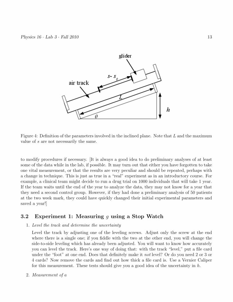
a = g sin θ = gh

L, (12)

where g = 9.80 m s−2, and L and h are simply geometrical quantities in a right triangledescribing the tilt of the track as shown in Fig. 4. The point here is that if we measure a, h,and L; then we can then compute g from Eq. 12.

3. We will assume that the kinematic relations for the case of constant acceleration are applicableto the motion of the cart on the airtrack. In particular, the coordinate position s of the cartas a function of time, t, on the track is described by

s = s0 + v0t+1

2at2. (13)

where s0 is the position at t = 0 and v0 is the velocity at t = 0.

Important Note: It is essential that you be prepared to calculate quickly the experimental val-ues of g from your observations, so that you can see how the results are coming out and be ready


Figure 4: Definition of the parameters involved in the inclined plane. Note that L and the maximumvalue of s are not necessarily the same.

to modify procedures if necessary. [It is always a good idea to do preliminary analyses of at leastsome of the data while in the lab, if possible. It may turn out that either you have forgotten to takeone vital measurement, or that the results are very peculiar and should be repeated, perhaps witha change in technique. This is just as true in a “real” experiment as in an introductory course. Forexample, a clinical team might decide to run a drug trial on 1000 individuals that will take 1 year.If the team waits until the end of the year to analyze the data, they may not know for a year thatthey need a second control group. However, if they had done a preliminary analysis of 50 patientsat the two week mark, they could have quickly changed their initial experimental parameters andsaved a year!]

3.2 Experiment 1: Measuring g using a Stop Watch

1. Level the track and determine the uncertainty

Level the track by adjusting one of the leveling screws. Adjust only the screw at the endwhere there is a single one; if you fiddle with the two at the other end, you will change theside-to-side leveling which has already been adjusted. You will want to know how accuratelyyou can level the track. Here’s one way of doing that: with the track “level,” put a file cardunder the “foot” at one end. Does that definitely make it not level? Or do you need 2 or 3 or4 cards? Now remove the cards and find out how thick a file card is. Use a Vernier Caliperfor this measurement. These tests should give you a good idea of the uncertainty in h.

2. Measurement of a


Put an aluminum riser block of your choice under the foot of the air track. Release the gliderfrom rest and time (using a stopwatch) how long it takes to travel a chosen distance s− s0.Use Eq. 13 to calculate a. Repeat 4 more times. Find the mean of the your five trials to getthe best value of a. The uncertainty on this value is given by the standard error. (For how tocalculate these values and other uncertainties refer to Appendix E.) Make sure each partnertakes their own data.

3. Best estimate of g

Now using your best values of h, L, a and Eq. 12, calculate the value for g. This is your bestestimate. Use the uncertainties of h, L, a and error propagation to determine the uncertaintyof g. The agreement with the standard value for g ought to be reasonably good. If youare off by 5% or more, you probably made a mistake somewhere in your measurements orcalculations. Check them over.

Q: What is the precision of your estimate? What is the accuracy of your estimate? (For thisquestion you will need to know the definitions of precision vs. accuracy before you come tothe lab.)

4. Correcting g

There are two main reasons why your preliminary measurement of g may be inaccurate:timing accuracy and air drag. The first reason is that your timing accuracy may be poor.It is clearly vital that the stopwatch be started and stopped “correctly.” If the watch is to bestarted upon release of the cart, and stopped when it hits the bottom of the track, these twoevents are qualitatively quite different: the start is rather slow, while the stop is quite fast.Thus, “reaction time” errors may not cancel out. The second reason is that air drag may besignificant and we assumed that frictional effects would be small. For a cart going downhill,air drag would tend to slow the cart down and to make the apparent value of g smaller thanexpected. To correct for this, start with the cart traveling uphill, and analyze a complete tripup and back down the track. Calculate your new g value; is it the same, larger, or smallerthan expected? Why?

Q: How could you limit the impact of these two errors on your measurement?

3.3 Experiment 2: Measuring g using a Motion Sensor

1. For your new experiment, initially use a 1′′ riser block.

2. Automate the timing technique

Use the motion sensor instead of a stopwatch. The motion sensor should be set to take 100readings at 0.2 sec intervals and situated ∼ 160 cm along the airtrack, with its height set sothat its center is ∼ 71

2cm above the track.

CAUTION: make certain that the cart on the airtrack never collideswith the motion sensor!


3. Release the glider and record data

Decide from where your glider will start and during which part of its motion you will recorddata. Then record the data using Data Studio. Have each partner record data.

4. Check your data quality

If you get a good quality position vs. time graph, you’re ready to analyze the data. If yourposition-time graph is “noisy”, try again. If you can’t eliminate the noise, see one of theinstructors. See Appendix A for data transfer instructions.

5. Analyze your data using a spreadsheet

Once you have a good graph, analyze part of your data as you did in the Bouncing Ball lab.That is select a good section of position vs. time data. Then create a velocity vs. time graphby calculating the mean velocity between consecutive points and the mean time betweenconsecutive points. Fit a line to the velocity vs. time data and extract the slope, this is g.Also, obtain a value for the statistical uncertainty in g by performing a linear regression andlooking at the statistics.

6. Calculate the experimental uncertainty

Consider all sources of uncertainty in each of the measured quantities that go into the deter-mination of g (see Appendix E in this lab manual) to estimate an experimental uncertaintyin g that is due to the apparatus and measurement technique.

7. Repeat with a different track angle

Repeat your experiment with the motion sensor using a different riser block, again acquiringone data set for each partner. You may need to change the motion detector time interval forthis set of measurements. Does your result for g improve? Why or why not?


4 Momentum: Elastic and Inelastic Collisions

Read the instructions completely and carefully before coming to lab. Also, work outhow to calculate the uncertainty in the momentum ratios (

pfpi

). You will need to workefficiently in this lab otherwise you may end up staying quite late.

4.1 Introduction

In this experiment we will use the conservation of linear momentum to study two types of collisions:perfectly inelastic collisions where the two colliding bodies adhere to each other upon contact andmove off as a unit after the collision, and perfectly elastic collisions, where the two collidingbodies bounce off one another upon contact and move as two separate entities after the collision.Linear momentum p for an object is equal to mv, where m is the mass of the object and v is theobject’s velocity. This means that a heavier or faster object will have more momentum than alighter or slower object. Since linear momentum is conserved, if objects collide, they can changetheir momenta, but the overall sums of the momenta have to be equivalent. This is given by theequation:

N∑i=1

pi,initial =N∑i=1

pi,final (14)

For two objects colliding in a perfectly elastic collision the equation becomes:

m1v1,initial +m2v2,initial = m1v1,final +m2v2,final (15)

and for two objects colliding in a perfectly inelastic collision the equation becomes:

m1v1,initial +m2v2,initial = (m1 +m2)vfinal (16)

4.2 Experiment: Elastic and Inelastic Collisions

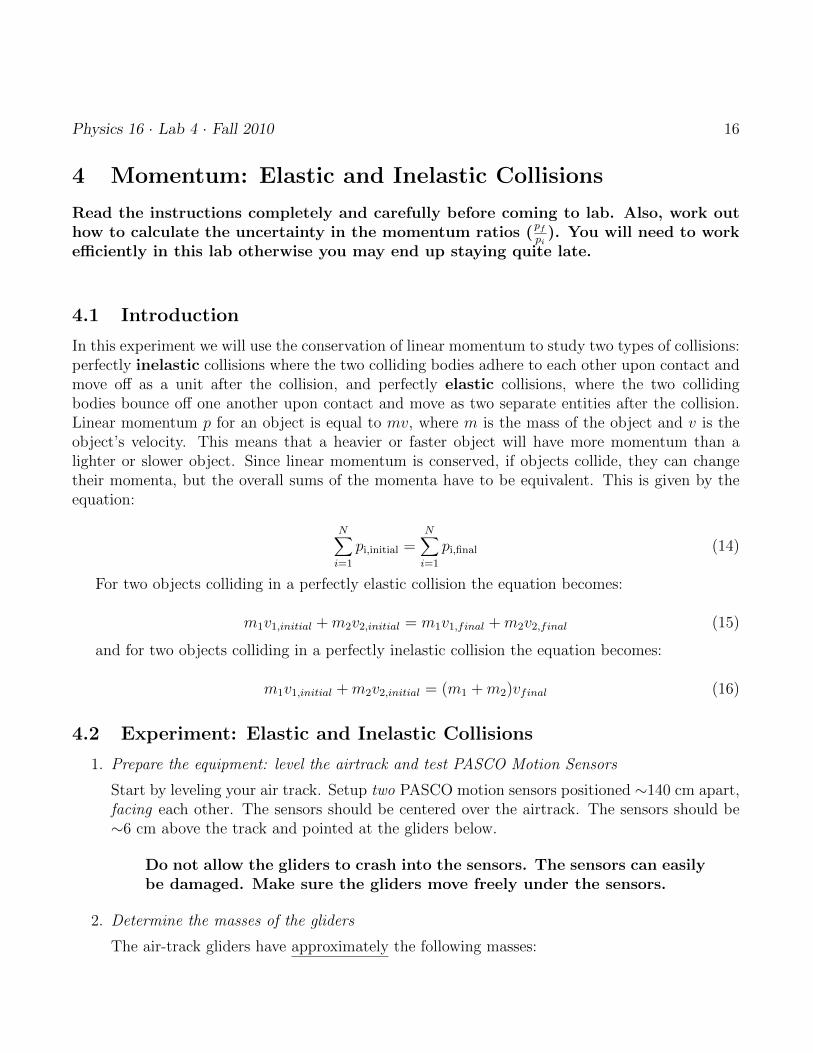
1. Prepare the equipment: level the airtrack and test PASCO Motion Sensors

Start by leveling your air track. Setup two PASCO motion sensors positioned ∼140 cm apart,facing each other. The sensors should be centered over the airtrack. The sensors should be∼6 cm above the track and pointed at the gliders below.

Do not allow the gliders to crash into the sensors. The sensors can easilybe damaged. Make sure the gliders move freely under the sensors.

2. Determine the masses of the gliders

The air-track gliders have approximately the following masses:


small glider 200 gramslarge glider 400 grams

You should check the masses of the carts you use on the electronic balance. List their massesand uncertainties here.

3. Test the motion sensors with a single glider

Push one glider along the length of the airtrack and record its position using both motionsensors. Remember, the sensors measure distances relative to themselves. Look at the graphof position vs. time. Based on your qualitative inspection of the graph, what can you sayabout the velocity of the single glider? The two plots from the two sensors will look verydifferent because one sensor will measure the cart as it comes closer to the sensor and the otherwill measure the cart as it gets farther away from the two sensors. How do you reconcile thetwo plots from the two sensors? Print out your plots and paste them into your lab notebook.

4. Measure the momentum transfer during a two body collision

Here we are going to measure the positions of two gliders colliding with each other and verifythat momentum is conserved. Place the small elastic glider at rest, between the sensors. Pushthe second small elastic glider into the first. Look at the graph of position vs. time for thetwo gliders.

Q: Can you identify the moment of collision?

Now use Data Studio to look at the velocity vs. time graph for the collision of the two gliders.Keep in mind that one of the sensors is looking backwards.

Q: How does this affect the velocity it measures? How will you correct the velocity?

Extract the initial and final velocities for each glider. List the velocities along with theiruncertainties in your lab notebook. Also, print out your plots and paste them into your labnotebook.

To verify that momentum is conserved, first calculate the total initial momentum of the twogliders before impact, pi. From the equations above this should be

∑Ni=1 pi,initial or in the

case of an elastic collision m1v1,initial + m2v2,initial. Second, calculate the final momentumof the gliders after impact, pf . Now calculate the momentum ratio,

pfpi

. Finally, use errorpropagation to calculate the uncertainty in the momentum ratio.

5. Repeat the two body collision measurement for 3 cases of collisions

For both elastic and inelastic collisions, you will investigate at least three cases (not necessarilyin the order given below). The minimum three cases are:

(a) small or large cart into another stationary cart of equal mass

(b) small cart into large cart at rest

(c) small or large cart into moving cart (equal or unequal mass)


This will give you a total of 6 data sets. You have already completed the data set for anelastic small cart bumping into an elastic small cart at rest. This leaves 5 data sets left todo. For each data set record the position vs. time data for the collision. Print the graphsand paste them into your lab notebook.

4.3 Analysis

For the 3 cases and 2 kinds of collisions (elastic and inelastic) you will have a total of 6 data sets.For each case, you should also extract the initial and final velocities and their uncertainties for eachcart. You can do this is one of two ways:

• Position vs. Time: for each data set there are 4 distinct line segments which represent the4 velocities of the gliders (2 before collision velocities and 2 after collision velocities). If theline segments are in fact lines, what can you say about the velocities? Use regression analysisto find the velocities of the gliders before and after the collision and the uncertainty.

• Velocity vs. Time: use the position vs. time data to calculate the velocity vs. time data asin the Bouncing Ball lab. Make graphs of velocity vs. time and identify the velocities of thetwo gliders before and after the collision. Make sure to calculate an average velocity for eachof the 4 velocity segments, the standard error will be the uncertainty.

Finally, calculate the final linear momentum (magnitude)/initial linear momentum (magnitude)(pf/pi) and its uncertainty for each case. Remember that the final momentum equation will bedepend on the type of collision: elastic or inelastic. Also, you must work efficiently if you don’twant to be here too late! Make sure to compile in your lab notebook a table of the ratios that youcalculate, along with their uncertainties.

Q: What is the expected ratio if momentum is conserved? Do your ratios agree with thisexpected ratio? Why or why not?


5 Conservation Laws: The Ballistic Pendulum (Formal Lab

Report)

Make sure to read and understand this handout in its entirety before coming to andbeginning the lab. Work out the derivations needed to complete the calculations in§5.2.

5.1 Introduction

The ballistic pendulum (see Fig. 5 below) was, once upon a time (before the era of high-speedelectronics), used to measure the speeds of bullets. The method used to determine the speed of thebullet depends on the clever use of fundamental conservation laws in physics.

Figure 5: Ballistic Pendulum

A bullet, with mass m and initial speed v, collides with and becomes lodged in a mass M .(See Fig. 6.) The larger mass M is supported as a pendulum. The collision itself takes place sorapidly that m and M together can be considered as a closed system during the collision, i.e. astwo particles which interact only with each other.

Immediately after the collision, the new composite object (m+M) has a velocity to the right,v′. Then (m+M) acts as a pendulum and swings upward, trading kinetic energy for gravitationalpotential energy. The amount of potential energy gained is given by (m + M)gh, where h is theheight through which the center of mass of (m+M) rises. In this lab you will calculate the muzzlevelocity v (or, more properly, the muzzle speed) of the bullet using a set of measurements of h.Using this information, you will then predict the range of the bullet (if it were not intercepted bythe ballistic pendulum) and you will dramatically test your prediction. Before class, you should

• derive an expression for v′, the speed of the composite object just after the collision, in termsof h and the masses. This can be done by considering the conservation laws which apply afterthe collision.


• relate v′ to the bullet’s muzzle velocity v by considering the conservation laws which applyduring the collision. Together with the previous expression, this gives an equation for v interms of h.

• predict how far the bullet would travel if it didn’t hit the pendulum and actually continuedunimpeded until it struck the floor a distance H below.

M M

Just before the collision

Immediately after collision

Pendulum atmaximum height

m

Centerof massv

m

h Mm

v’

Figure 6: Ballistic Pendulum before and after collision

5.2 Experiment: The Ballistic Pendulum

Predict the horizontal distance, H, the bullet will travel before striking the floor. Start by doingthe derivation outlined below using only variables (before coming to lab), then measure values forthe various parameters. Once you have a predicted range and its uncertainty, test your prediction.

1. Measure h and its uncertainty

Be careful to measure h properly. For a point mass, the change in the gravitational potentialenergy is ∆U = mgh. For an extended object, this same expression holds if h is the changein vertical position of the center of mass.

There is a set of notches to catch the pendulum at approximately its highest point. Thenotches are numbered but the numbers are simply labels. You must measure the appropriatevalue of h directly with a caliper.

You will want to make a series of measurements of h (at least 7) in order to determine itsuncertainty.

2. Weigh the projectile (m) and the pendulum bob + hanger (M)

The bullet can be weighed. Make sure you keep track of your bullet as its mass (m) isimportant and the bullets don’t all have the same mass.


The larger mass M can also be removed from the pendulum for weighing.

3. Calculate the horizontal range, H, of your projectile

Don’t forget to calculate the uncertainty!

4. Mark your prediction

Tape paper and carbon paper to the floor so that the bullet makes a distinct mark. Markthe expected impact point and the uncertainty range.

5. Test your prediction

Be careful! The bullets move at fairly high speeds.

Summon one or more of the instructors and let us see how good your prediction is. Whentesting your prediction, do not be confused by bounces!

Carry out a series of trials (at least 5) of the horizontal range of the bullet as a projectile.Record the actual distance the bullet travels for each trial, and compare with prediction.

5.3 Formal Report

Your write up should focus on how you measured each of the relevant quantities and how youdetermined the uncertainty for each of them.

• Explain carefully how you used the observed value of h to calculate v and how you used thisvalue to predict the horizontal range.

• Describe how well you did at predicting the horizontal range. (Uncertainties for the ex-pected and measured values of the horizontal range should be included.) Do you notice anytrends in your data, anything systematic? If so, comment on this.

• Discuss the conservation or non-conservation of kinetic energy in this collision. Was thekinetic energy of (m+M) just after the collision equal to the kinetic energy of the bullet justbefore the collision? If not, what percentage of the bullet’s initial kinetic energy waslost?

Read Appendix D for important instructions concerning formal lab reports.


6 Rotation: The “Outward Force” Apparatus

Make sure to read and understand this handout in its entirety before coming to andbeginning the lab. You will conduct this experiment twice, for two different angularvelocities.

6.1 Introduction

6.1.1 Background on Rotational Motion

Consider a body in uniform circular motion as shown in Fig. 7. The body might be, for example,a ball on the end of a string. We know from kinematics that a body in uniform circular motionis accelerated: although the speed remains constant, the velocity vector is continually changing indirection. We also know that the acceleration is a vector directed toward the center of the circlewith a magnitude of

ac =v2

r=

4π2r

T 2, (17)

where r is the radius of the circle, and T is the period of the circular motion.

5-1

Lab #5 The “Outward Force” due to Rotation

(Informal) NOTE: Make sure to read and understand this handout in its entirety before coming to and beginning the lab. You will conduct this experiment twice, for two rotation speed settings. Consider a body in uniform circular motion as shown in Fig. 1. The body might be, for example, a ball on the end of a string. We know from kinematics that a body in uniform circular motion is accelerated: although the speed remains constant, the velocity vector is continually changing in direction. We also know that the acceleration is a vector directed toward the center of the circle with a magnitude of 2 2 2= / 4 /ca r r Tυ π= , where r is the radius of the circle, and T is the period of the circular motion.

From our study of dynamics we know that the acceleration a body experiences can be predicted from a knowledge of the forces acting on it. What are the forces acting on the ball? The string is surely pulling on it; so, there is an inward force of magnitude Fin as shown in Fig. 2. Childhood experience also leads us to suppose there is an outwardly directed force, whose magnitude is labeled X in the diagram. But how large is X? In this lab, we will suppose that there is indeed an outward force experienced by a body undergoing uniform circular motion. We will do this as a means of reconciling some perhaps preconceived notions about “centrifugal force” with the existence of actual forces in such a system. Presuming the existence of X, the net inward force would be Fnet = Fin - X, and we can use Newton’s Second Law to write

Fnet = Fin – X = mac or

2

24 in

rX F mTπ

= − . (1)

In this experiment, instead of using a ball on the end of a string, we will use a cylindrical

Figure 7: Body in circular motion and its force diagram

From our study of dynamics we know that the acceleration a body experiences can be predictedfrom a knowledge of the forces acting on it. What are the forces acting on the ball? The string issurely pulling on it; so, there is an inward force of magnitude Fin as shown in Fig. 7. Childhoodexperience also leads us to suppose there is an outwardly directed force, whose magnitude is labelledX in the diagram. But how large is X? In this lab, we will suppose that there is indeed an outwardforce experienced by a body undergoing uniform circular motion. We will do this as a meansof reconciling some perhaps preconceived notions about “centrifugal force” with the existence ofactual forces in such a system. Presuming the existence of X, the magnitude of the net inwardforce would be Fnet = Fin −X, and we can use Newton’s Second Law to write

Fnet = Fin −X = mac (18)


and therefore

X = Fin −m4π2r

T 2. (19)

In this experiment, instead of using a ball on the end of a string, we will use a cylindrical massattached to a spring. The only property of the spring we need to know is that, by Hooke’s law, theforce exerted by the spring (that is, Fin in Fig. 7) depends only on how much the spring is stretched.Thus Fin can be measured (using the apparatus described below) by a separate experiment in whichthe spring is stretched by the same amount as under rotating conditions. Since Fin, m, r, and Tcan all be measured, Eq. 19 can be used to determine the experimental value of X. The key toachieving sensible results will be in thoughtfully determining uncertainties in all measured values,as described later in these notes. Make sure to pay special attention to this aspect of the experimentas you go along.

6.1.2 Description of the “Outward Force” Apparatus

Figure 8: View of entire apparatus

The outward force apparatus (Figure 8) is an experiment that allows you to calculate both theforce acting on a rotating mass and the acceleration of the rotating mass independently. This isimportant because we want to compare Fin and mac so we need independent measurements of forceand acceleration.


Figure 9: Cross-section view of the carriage attached to the rotation device

The apparatus consists of a carriage, as shown in Figure 9, that holds a mass connected to aspring. The mass is attached to the spring, but is otherwise free to slide back-and-forth in thehorizontal direction within the carriage cylinder. The carriage has a small vertical rod that isattached to its base and fits into the cylindrical holder at the bottom of the picture in Figure 9.This cylindrical holder is the rotator shaft. The thumbscrew on the rotator shaft screws in totighten the vertical rod and secures the carriage to the rotator shaft. The rotator shaft is attachedto a rotator device, as shown in Figure 8, that spins the entire carriage at various constant speeds.From the angle of this picture the device would rotate the carriage in and out of the page. Thisrotation causes the mass to slide outward increasing the distance from the center of rotation andalso activating the spring. In the picture, the mass is fully extended to the outermost position. InFigure 10, the mass is in it’s innermost position and is still stretched. The rest position of the masscorresponds to the center of the carriage, which also happens to be where the axis of rotation is.

Figure 10: Cross-section view of the carriage


The way the apparatus allows for independent measures of force and acceleration is by measuringacceleration using uniform circular motion described in Eq. 17, and by measuring force using theextension of a spring. First, let’s describe how we measure acceleration using the apparatus. Forany particular (constant) speed, the period of rotation (T ) is constant, and the mass (m) rotatesat a constant distance (r) from the center, corresponding to uniform circular motion. You willmeasure the period of rotation by using a stop watch and a counter that counts the number ofrotations. The distance, r, you will measure with a vernier caliper. Using these two values you cancalculate the acceleration, ac, from Eq. 17. Second, to find the force you measure the extension ofthe spring during rotation, which happens to be r, as well. Then you take the carriage off of therotation device and attach a weight to the spring to extend it the same distance r. The force dueto the weight is then your force, Fin. Finally you can compare mac and Fin to see if they are thesame, or if there is a mysterious centrifugal force, X.

6.2 Experiment: Measuring the Mysterious Centrifugal Force of “Murky”Origins

1. Make a hypothesis about X

First, draw a free body diagram of the mass in the carriage. Pay particular attention to thedirection of Fin. What is the direction of ac? From this free body diagram do you expect anonzero X force?

2. Assemble the apparatus

There is a thumbscrew at the far right in Fig. 9 that is attached to the spring in the carriage.Tightening or loosening this spring thumbscrew will change the spring tension. Begin withthe spring thumbscrew screwed in as far as possible. Extending from the carriage is an 8 mmdiameter cylindrical vertical rod, as described above, with one flat face. Mount the carriageon the rotator device by inserting this rod into the rotator shaft and tightening a lockingthumbscrew (this is a different thumbscrew from the spring thumbscrew in the carriage). Besure that the locking thumbscrew presses against the flat face of the rod.

3. Adjusting the rotation rate and measuring the period (T ) and mass distance (r)

The rotation rate can be controlled by the experimenter by an adjustment thumbscrew, whichis at the bottom left corner in Figure 8. As you move the thumbscrew the position of a crankshaft on a rotating wheel changes. The velocity is greatest at the edge of the wheel so movingthe adjustment thumbscrew such that the crankshaft moves down, toward the edge of thewheel increases the rotation rate. The period T can be measured with a stopwatch and acounter by counting the number of revolutions occurring during a set time period. (Use afairly large total time in order to minimize the effect of error due to your reaction time instarting and stopping the stopwatch.) The counter is located just below the rotator shaft andthe locking thumbscrew. To avoid the problem of trying to determine r while the apparatusis in motion, a pointer device is built into the apparatus. You can adjust the rotation so that


the mass assumes the value of r needed to just activate the pointer. The pointer is locatedin the carriage, on the left side, just below the spring and mass. The point of the pointer isin the center of the carriage, right next to a small cylinder. If the pointer is not activatedthe pointer points to the bottom of the carriage and cylinder. If the pointer is just activatedit points to the top of the cylinder as in Figure 9. If the pointer is overly activated then itpoints to the top of the carriage above the cylinder.

You will make three measurements of T at three different rotation rates:

i. Measure the “best” rotation rate, at which the mass barely activates the pointer.

ii. To get an upper bound, find the lowest rotation rate at which the pointer is consistentlyin the “up” position. Note that rotation rates higher than this will also give a consistent“up” position because the mass becomes pinned against the end of the carriage. Theidea is to place your upper bound as close to your “best” value as possible.

iii. Place a lower bound by finding the highest rotation rate at which the pointer is consis-tently in the “down” position.

4. Measure r

To measure the r where the pointer is just activated, you need to use a fun little screw gadget.With this gold colored screw gadget you can hook your spring to the gadget and by screwingin a screw pull the mass so that the pointer is just activated. Then you can use calipers tomeasure the distance from the axis of rotation (center of the carriage) to the center of mass.Since this mass is not a point mass, the manufacturer has obligingly marked a line on it toindicate its center.

5. Calculate ac and mac

From the measurements described above, compute the magnitude of the centripetal accelera-tion, 4π2r

T 2 , and compare it to the familiar acceleration due to gravity, g, to get a feel for howlarge ac is in this particular rotating system.

6. Determine Fin

To determine the magnitude of the force Fin exerted by the spring when m is in the criticalposition that actuates the pointer, you can suspend the carriage vertically and attach hangingweights until m is pulled down the appropriate distance. Be sure to determine an uncertaintyfor this quantity as well.

7. Repeat the experiment twice

Repeat the experiment with the spring thumbscrew at its maximum point away from thecarriage side, and again with the screw halfway between maximum and minimum positions.


6.3 Analysis

Make a plot of Fin vs. mac. Be sure to include error bars that account for the combined uncertaintiesof all variables used to calculate Fin and mac. Is your data consistent with the equation Fin = mac,or do you find evidence for a nonzero X force? If there is no outward centrifugal force, X, thenwhy does the mass extend outward when you rotate the carriage?


7 Static Equilibrium: The Force Table and the Moment of

Force Apparatus

7.1 Introduction

Static equilibrium is governed by two equations. The first is that the sum of the forces (F ) actingon a static object must equal 0, or

∑Ni=1 F = 0. This means that a static object does not translate.

The second is that the sum of the torques (τ) acting on a static object must equal 0, or∑Ni=1 τ = 0.

This means that a static object can’t rotate. In this lab we will use both of these principles andvector algebra to measure, calculate, and experiment with objects at rest.

The force table apparatus (Fig. 11) provides a simple means for testing that the sum of theforces on a static object must be zero. The face of the table is a heavy metal disk calibrated aroundthe edge in degrees (360◦ total). A brass ring, held near the center of the table by a vertical pin,carries three attached strings, each of which can be directed over a pulley fixed to the table edgeand terminated with a hanging weight pan. The addition of weights to these pans creates a tensionin each string. Each string is thus said to pull on the brass ring and create a force. By using vectoralgebra we should be able to create positions where the three forces cancel one another and thebrass ring remains in the middle of the table.

Figure 11: Force Table

The moment of force apparatus (Fig. 12) allows us to test the second governing equation thatthe sum of the torques on a static object must be zero. The torque, τ , or moment of force asengineers call it, is caused by a force, F , acting at a distance from the axis of rotation, x, and isgiven by:

τ = Fx sin(θ) (20)

where θ is the angle between the force and the distance vector. See Fig. 13. In the moment of forceapparatus a torque is created by hanging a weight from a ruler that is balanced on a knife-edgecalled a fulcrum. Weights can be suspended from the ruler at different positions causing the forceto act at different distances from the fulcrum, creating various torques on the ruler. By calculating


the different forces due to the weights and measuring the distance along the ruler we can calculatethe individual torques and create arrangements where the ruler is in static equilibrium.

Figure 12: Moment of Force Apparatus from the Cenco catalog

Figure 13: Diagram of the definition of torque

7.2 Experiment 1: The Force Table

Examine the force table example set up in the lab in order to appreciate what your goal will be.Notice that if the weights and string angles are adjusted just right, you can remove the restrainingpin, and the ring is held in equilibrium by the action of the three string forces alone. See Fig. 14.However, there is nothing unique about the choices used in the example: there is an infinity ofcombinations of “string-directions-plus-weights” that will permit equilibrium of the ring. Yourtask is to show that for other combinations, your chosen values are explained by vector algebra.

7.2.1 Procedure

The procedure consists of two trials:

1. For the first trial, you will experimentally determine a force that moves the ring into staticequilibrium.

(a) Decide on weights and angles for two of the strings. Start with at least 100 grams oneach of the two strings. Do not use bare hangers and do not neglect the weight of thehangers. The two positions you select will remain fixed during the rest of the trial. Ifyou wish, you may use “easy” angles like 0◦ and 90◦, or 0◦ and 120◦.


Figure 14: Top view of the force table

(b) Without prior calculation, apply a weight to the third string and vary its magnitude andangle until the third string balances the forces exerted by the first two.

(c) Once you have verified that the balance is “pretty good”, estimate uncertainty by addingor subtracting weight until the ring has moved noticeably off-center, or by moving theangle in both directions until the ring is off center.

(d) Finally, verify your experimentally determined force. Using the weights and angles forthe first two strings, either numerically or graphically, calculate the third force on thering.

2. For the second trial, you will calculate the theoretical magnitude and direction of the thirdforce before you test to see if your calculations are consistent with experiment.

(a) Choose two new weights set at new angles. Do not separate the first two strings by“easy” angles like 90◦. The strings should also be weighted with unequal masses.

(b) • One of the lab partners should conduct a rough graphical analysis (using a rulerand protractor) to calculate the third force with a scale drawing.

• The other partner should conduct a numerical analysis (using trigonometry). Toguide your application of vector algebra to this situation, we recommend that youmentally impose an XY-coordinate frame on the table face with the origin at thetable center, and one axis aligned with the zero degree marker.

7.2.2 Results

The results should now be compared and any differences reconciled. For each trial list the resultsin a table, like the one below. Note that in this example case there is not good agreement betweenthe predicted and measured results. Thus, some further investigation is needed. Explain in yourlab notebook why there might be any discrepancies.


Magnitude (N) Direction (degrees)Theory (graph) 2.30 120Theory (numerical) 2.31 119Experiment 2.05± .02 129± 2

7.3 Experiment 2: The Moment of Force Apparatus

Your goal in this experiment will be to balance a ruler while various weights exert different torques,just like in the last experiment the goal was to balance the center ring while different weightsapplied different forces. Again there are many combinations that will allow the ruler to remain instatic equilibrium; your job will be to find two ways. Remember that the force being exerted onthe meter stick by a weight with mass, m, has a force equal to mg. The distance vector, x, can bedetermined by the ruler itself. The angle, θ, will always be 90◦ so that τ = mgx.

7.3.1 Procedure

The procedure consists of two trials:

1. For the first trial, you will experimentally determine the balancing torque.

(a) First, place the hanger with the 50 cm mark at the center of the fulcrum and check tomake sure it is balanced. Why is this the case? Note: some of the rulers may be a littlebeat up, so the point of balance might be slightly off from the 50 cm mark. If it is >1cm from the 50 cm mark, please get another ruler, as the uneven mass of the ruler itselfwill throw off your calculations.

(b) Second, add a hanger with a weight on it. Do not use bare hangers. This weight willremain fixed during the trial. Write down the mass, position, and torque due to theweight.

(c) Without prior calculation, apply a weight to the other side of the ruler (with a differentmass from the first weight) and vary its magnitude and distance until the ruler balanceson the fulcrum.

(d) Once you have verified that the balance is “pretty good”, estimate uncertainty by addingor subtracting weight until the ruler has moved noticeably. Also move the distance inboth directions until the ruler begins to swing.

(e) Finally, verify your experimentally determined torque. Using your initial torque and thesecond weight’s mass, calculate the second torque and the distance of the second weight.

2. For the second trial, you will calculate the theoretical magnitude and direction of the secondtorque before you test to see if your calculations are consistent with experiment.

(a) Add a different weight to the ruler at a new distance. Write down the position of thefulcrum, the distance from the fulcrum to the weight, the mass of the weight, and theinitial torque.


(b) Now calculate the magnitude and direction of the second torque. The direction tells youwhich side of the ruler to place the weight, why? Next pick a particular mass (hanger +weight) that is different from the first weight and calculate the distance from the fulcrumthat you should place the mass to get the second, balancing torque.

(c) Verify your calculation experimentally.

7.3.2 Results

Again let’s compare the theoretical and experimental results in a table, like the one below. Werethere any disagreements? Why?

Second Torque Magnitude (N·m) Second Weight Distance (m)Theory 0.54 0.054Experiment 0.50± 0.05 0.057± 0.012


8 Fluids: Venturi Meter and Artificial Heart

8.1 Introduction

The aim of this lab is to give you some experience with fluid dynamics. Probably, the mostimportant principle in physics that is used in medicine is Bernoulli’s equation. Bernoulli’s equa-tion describes the pressures and velocities of fluids in a pipe, a model for blood in your arteries!Bernoulli’s equation is:

p+ ρgy +1

2ρv2 = constant (21)

where p is pressure, ρ is fluid density, g is the acceleration due to gravity, y is the height of the fluid,and v is the fluid velocity. If there is no elevation change, then the pressure in the pipe becomesdirectly related to the velocity in the pipe by:

p+1

2ρv2 = constant (22)

This tells you that as pressure increases, velocity decreases and vice versa. So if you happen tohave high blood pressure then that means that the velocity of the blood in your arteries will besmaller than normal, causing your heart to work harder and taking longer for oxygenated blood toreach your extremities.

Now let’s think about atherosclerosis or hardening of the arteries where the artery becomesconstricted. This is analogous to decreasing the radius, r, of a pipe. What happens to your bloodpressure and velocity when this happens? First, let’s look at velocity. Remember that the flow rate(Av, where A is the area of the pipe) through a pipe is constant. This is given by the equation ofcontinuity:

A1v1 = A2v2 (23)

r12v1 = r2

2v2 (24)

From this equation we can see that as the radius decreases, the velocity in the pipe goes up.According to Bernoulli’s equation a velocity increase would lead to a pressure decrease. At firstthis may seem counter-intuitive since atherosclerosis increases the likelihood that the artery willburst, causing a heart attack or stroke. But the artery does not burst due to the blood pressure inthe constriction, it bursts because of the pressure the plaque exerts on the arterial wall or becausea completely blocked artery would create an increase in blood pressure in the chamber before thebuild-up, akin to filling up a water balloon until it burst.

8.2 Experiment 1: Venturi Meter

Here we will use a venturi meter to measure velocity flow rate, Av. A venturi meter is a tube witha constricted throat that increases velocity and decreases pressure, as we described above. Theyare generally used to measure flow rates of fluids in a pipeline, like in a sewer system. They canalso withstand very cold temperatures due to their lack of moving parts and are used in the oilpipelines in Alaska.


1. Measure the radii of the chambers in the venturi meter

Measure the outer diameters (ODs) of the first two chambers at the top of the venturi meterwith a caliper. Also measure the wall thickness and subtract this quantity correctly to getthe inner diameter (ID). Then find the radii of the two chambers, r1 and r2. Estimate youruncertainty and be sure to correctly propagate it to the measurement of the radius.

2. Setup the apparatus to measure the flow rate of an air line

Fill the bottom of the venturi meter a third of the way full with water. Then connect thebottom of the meter to the top of the meter. Keep the meter level with the table. Connect a1/2” OD clear tube from the meter to the air line. Leave the other end of the venturi meteropen to the atmosphere.

3. Find the pressure difference inside the meter

Turn on the valve to the air line and watch the water in the tube. It should begin to rise orfall based on the pressure in the chamber. If the pressure in the constriction decreases relativeto the first chamber, then it won’t be able to “push” down as hard on the water relative tothe first chamber. Write down in your notebook what the water levels in the bottom part ofthe meter look like. Make sure also to measure their heights (with the uncertainty). Whatdoes the water height say about the pressure in the chambers in the top part of the meter?

Now calculate the pressure change between the constriction and the first chamber, p2 − p1.To do this, solve Bernoulli’s equation for the pressure change on the water in the bottom ofthe meter. Find an expression for the pressure change in terms of the heights of the water.Record this pressure change and the calculated uncertainty.

4. Calculate the flow rate

Using this pressure change you can calculate the velocity of the air inside the meter. To dothis, solve Bernoulli’s equation for the pressure change on the air in the top of the meter. Youshould find an expression that relates the pressure change to the velocity in the first chamberv1, and to the radii of the first two chambers, r1 and r2. Since the pressure change on theair is the same as the pressure change on the water, you can now rearrange the equation tosolve for the velocity. The flow rate is then just A1v1. Record this quantity along with itsuncertainty.

5. Repeat the procedure for two more flow rates

Change the flow rate by turning the valve and remeasure the appropriate variables alongwith their uncertainties. You want to get to the point where you can do this rather quickly.I recommend typing all of the values into google (yes google is a calculator too) so that youonly have to type in the height difference to get the velocity.

Q: Why can we only measure the flow rate out of the airline, not the actual velocity?Q: Could you use the venturi meter to measure absolute pressure? Why or why not?


8.3 Experiment 2: Artificial Heart

In this section of the lab we will use an artificial heart to measure some physical properties of“blood” flow in the body. Our artificial body consists of a heart that pumps “blood” into thearteries; the “blood” then returns back to the heart via the veins. Here the artificial heart is adiaphragm pump, which is a rubber membrane with an attached handle and two one-way valves.This is a surprisingly good model of one side of the heart. The heart consists of two sides right andleft. The right side takes the blood from the body through the veins and pumps it to the lungs,the left side takes the now oxygenated blood from the lungs and pumps it through the arteries intothe body. Here we have simplified things by excluding the lungs so that only one pump is needed.Each side of an actual heart has two chambers and two one-way valves. The way the actual heartpumps is that the first chamber, the atrium expands filling with blood. As the atrium contracts thefirst one-way valve is opened and the blood enters the second chamber, the ventricle. The ventricleis expanding at this time, which also draws the blood into the chamber. Then the ventricle beginsto contract closing the first one way valve and opening the second, pumping the blood out of theheart. Our artificial heart is simplified so that it doesn’t include the atrium. After the heart, inour artificial body, we also have a system of arteries that can have different constrictions to modelhardening of the arteries.

1. Measure the flow rate of the artificial heart

To measure the flow rate of the artificial heart connect the venturi meter to the pump. Haveone partner steadily pump the diaphragm while the other partner measures the water levels inthe venturi meter. Use the water level measurement and the Bernoulli equation to calculatethe flow rate. Is the flow rate constant? How does the flow rate of the artificial heart compareto the flow rate of an actual heart? (A normal heart pumps 5 L of blood per minute and 1cm3 = 1 mL.)

2. Measure the blood pressure of the artificial heart

A blood pressure measurement is usually given as the systolic pressure over the diastolicpressure in mmHg. Systolic pressure occurs when the ventricle ejects the blood (in our casewhen the diaphragm membrane contracts) and represents the highest blood pressure that canoccur. Diastolic pressure is the lowest pressure in the cycle and occurs when blood is enteringthe ventricle (in our case when the diaphragm membrane expands). Observe your artificialheart to see if this is true.

Now let’s measure artificial blood pressure. Disconnect the venturi meter so the part withthree long tubes is not present. Then connect the PASCO pressure sensor to the first chamber.To connect the sensor to the computer see Appendix A. Pump the “blood” and look at theoutput of the pressure sensor. How does the pressure on the sensor relate to the “blood”pressure? Take the maximum pressure and convert it to mmHg as well as the minimumpressure. How does this compare to a normal blood pressure of “120 over 80” or 120 mmHg/80 mmHg?


3. Measure the flow rates in arterial branches

In the body your arteries branch out carrying blood to different parts of the body. How doesa branch affect the flow rate? Connect the venturi meter to one branch of the artificial artery.Keep all four branches open and monitor the flow rate. Now close one of the other branchesand watch what happens to the flow rate. Next close two of the other branches, then all threeof the other branches. What happens to the flow rate? Describe your observations using anequation.

4. Measure how a constricted artery affects the blood velocity in an arterial branch

In the body some of your arteries may have atherosclerosis (hardening of the arteries), orsome may just be bigger than others. To simulate different sized arteries you can turn thevalves to constrict the flow so as to model a smaller artery. Play around with this. How doesflow rate and velocity change in an arterial branch when one of the branches is constricted?


9 Waves and Oscillations: Simple Harmonic Motion and

Standing Waves (Formal Report)

Make sure to read this lab in its entirety before coming to and beginning the lab.Before coming to lab, you must do the following exercises.1. Substitute Eq. 27 into Eq. 26 (you will need to evaluate the second derivative ofEq. 27) and verify that Eq. 27 provides a solution to Eq. 26.2. Find a relationship that expresses the period, T , as a function of the mass, m, andthe spring constant, k.3. Substitute Eq. 31 into Eq. 30 and show that Eq. 31 is a solution of Eq. 30 and fromthis determine the relationship between ω, g and L.

9.1 Introduction

9.1.1 Simple Harmonic Motion

In this experiment you will explore two situations which give rise to simple harmonic motion (SHM).The common characteristic of both situations is that an object is acted on by a force which increaseslinearly as the object moves away from an equilibrium position:

Fx = −kx, (25)

where x is the displacement from the equilibrium (Fx = 0) position. Such a force is called arestoring force since the force tends to pull the object back to the equilibrium position. The fartherthe object is away from equilibrium, the larger the force pulling it back.

The motion of an object acted on by such a force is described by a differential equation of theform

d2x

dt2= −ω2x, (26)

where, as above, x is the displacement of the object from its equilibrium position, and ω is aparameter called the angular frequency. The solution of this differential equation, assuming that xis at its maximum value at t = 0, is

x(t) = A cos(ωt), (27)

where the amplitude, A, is the maximum displacement of the system from its equilibrium position.An important property of simple harmonic motion is that ω is independent of A. The period ofthe oscillation is given by

T =2π

ω. (28)

In this laboratory you will be investigating the extent to which the oscillatory motion of apendulum and of a mass on a spring can be described as simple harmonic motion.


Motion of a mass on a spring A spring provides one of the simplest examples of a linearrestoring force. The simplest case occurs when the motion is horizontal and the mass slides on ahorizontal frictionless plane. Having few such planes available, we will instead study the verticalmotion of a mass suspended from a spring. The vertical position of the mass is an oscillatoryfunction of the form

y(t) = y0 + A cos(ωt) (29)

This is similar to Eq. 27 except that the initial displacement, y0, is not zero.

The Simple Pendulum For small oscillations, the angular displacement of the pendulum, θ, isdescribed by the equation

d2θ

dt2= − g

Lθ. (30)

Note that Eq. 30 has exactly the same form as Eq. 26. Hence, we may immediately concludethat the angular displacement described by θ(t) will execute simple harmonic motion

θ(t) = θ0 cos(ωt) (31)

whereω2 =

g

L. (32)

9.1.2 Standing Waves

In this experiment, you will set up standing waves on a string by mechanically driving one end ofit. As you change the driving frequency, you will observe the phenomenon of resonance. As thedriving frequency approaches the resonant frequency the string will start to vibrate with a largeamplitude. You will in effect set up standing waves along the string that you can measure thewavelength and frequency of.

The theory (covered in lectures) relates the wavelength and frequency of standing waves to thespeed of propagation of waves in the medium (the string, in our example):

v = λf (33)

where v is the speed of the wave, λ is its wavelength, and f its frequency.Theory also relates the speed of propagation of waves in a medium to the properties of the

medium. Typically, the wave speed is the square root of an elastic property of the medium such asa tension or stress divided by an inertial property such as mass density. In the case of waves on astring, the speed is given by

v =

√F

µ(34)

where F is the tension in the string, and µ is its mass per unit length. (We reserve the letter Tfor period, and hence don’t use it for the tension in the string here). In the lab, you will choose


one value of F , and make a measurement of the wavelength of the standing waves for at least oneresonant frequencies. Other groups will measure the same properties at different tensions. For agiven tension, your data will allow you to investigate Eq. 33. The calculated average value of thevelocity for each of the different tensions will permit a test of Eq. 34.

9-2

The places where the wave disturbance is zero are called the nodes and the places where the disturbance is a maximum are called antinodes. One may think of a standing wave as the sum of two traveling waves, one traveling to the right and the other to the left. The distance between two successive nodes (or two successive antinodes) in a standing wave is half the wavelength of either of the traveling waves that comprise the standing wave. Clearly the fixed ends of the string are always nodes. With that constraint, the longest wavelength standing wave corresponds to n = 1 in the figure, and is variously called the fundamental or the ‘lowest note’ or the lowest mode of the string, the latter terms coming from the fact that the frequency is smallest for these standing waves. The higher n values correspond to harmonics of the fundamental, the overtones. Mathematically, it is not hard to check that

2 /n L nλ = , (3) where n is the number of antinodes in the standing wave pattern. The frequencies are given by

1.nn

f nfυλ

= = (4)

We should note that the string does not have to vibrate so that it has only one of these basic

patterns of standing waves. In general, the excitation of a string (like that of a stringed instrument) will produce a mixture of these different patterns with different amplitudes simultaneously. The mix of overtones, among other features, distinguishes a violin from a piano or other instruments all playing the same “note”, and lends music a richness that is hard to capture by our simple analysis. Still, understanding of the pure modes allows us to analyze even highly complicated mixtures of modes.

III. Procedure To begin, you will need to determine the linear mass density µ of the string that you will be

using. Cut a piece of string at least 4 meters in length and measure its length as precisely as you can. Then measure the mass of the string using the high-precision scale. Now cut the string to a length somewhat longer than the workbench, tie one end to a post at one side of the workbench, pass the other end of the string over a pulley at the opposite side of the bench and attach a hanger to it.

Figure 15: Standing waves on a string. n=1 corresponds to the fundamental mode; n>1 areharmonics.

When the string is held (more or less) fixed at the two ends, the standing wave patterns shownin Figure 15 are possible. The places where the wave disturbance is zero are called the nodes andthe places where the disturbance is a maximum are called anti-nodes. One may think of a standingwave as the sum of two traveling waves, one traveling to the right and the other to the left. Thedistance between two successive nodes (or two successive anti-nodes) in a standing wave is halfthe wavelength of either of the traveling waves that comprise the standing wave. Clearly the fixedends of the string are always nodes. With that constraint, the longest wavelength standing wavecorresponds to having an anti-node n = 1 in the figure, and is variously called the fundamental orthe “lowest note” or the lowest mode of the string, the latter terms coming from the fact that thefrequency is lowest for these standing waves. The higher n values correspond to harmonics of thefundamental, the overtones. Mathematically, it is not hard to check that

λn =2L

n. (35)

The frequencies are given by

fn =v

λn= nf1. (36)

We should note that the string does not have to vibrate so that it has only one of these basicpatterns of standing waves. In general, the excitation of a string (like that of a stringed instrument)will produce a mixture of these different patterns with different amplitudes simultaneously. Themix of overtones, among other features, distinguishes a violin from a piano or other instruments allplaying the same “note”, and lends music a richness that is hard to capture by our simple analysis.


Still, understanding of the pure modes allows us to analyze even highly complicated mixtures ofmodes.

9.2 Experiment 1: Mass on a Spring

1. Study and measure the period

Choose one of the two conic shaped masses provided and attach it to the spring. Measurethe mass. Note: in is important to record the mass of the spring itself. In all calculationsinvolving the oscillating mass, use the total mass:

mtot = mhanging +1

3mspring (37)

Measure the period of oscillation.

Q: Why is it better to determine the time for 50 oscillations than for just 5?

Carry out measurements for at least different 3 amplitudes to see if the period is indepen-dent of the amplitude of the motion as predicted. Make sure you stay in the limit of smalloscillations (< 15 cm). Record the values of the amplitudes you use.

2. Determine the spring constant

From your period measurements, determine the spring parameter, k.

3. Repeat for the second mass

Attach the second mass to the spring and measure the period of its motion. Determine thespring parameter, k, from these measurements.

Q: For the two masses you used above, what should the ratio of the periods be? Calculatethe ratio of the measured periods, and compare it with the predicted ratio. Do they agreewithin uncertainty? If not, why not?

4. Hooke’s Law

To test Hooke’s Law make a series of measurements of the stretch of the spring, x, vs. theapplied force, F = mg. Hang a mass hanger on the end of the spring. Starting with 100g,add mass to the hanger and measure the length of the spring. Make several measurementsbetween 100-800g. Plot F vs. x. Describe qualitatively the relation between the weight andlength of the spring.

Q: What range of values does the spring obey Hooke’s Law?

Determine the spring constant k using regression analysis. Compare the value obtained withthe values determined in steps 2 and 3.


5. Measure the parameters using a motion sensor

Set up a motion sensor to observe the position of an oscillating mass as a function of time.In the equilibrium position, the mass (about 450 g) should be about 70 cm above the sensor.You may have to try more than one combination of sample interval and number of samplesbefore finding a good one.

(a) Use the motion sensor to measure the position of the mass for a ∼5 second intervalafter you have displaced the mass about 5 cm from its equilibrium position and carefullyreleased it. Do not start the motion sensor until after you have released the mass andmoved well away from the experimental apparatus. Make certain no one is leaning onthe table during the measurement.

(b) Look at the graph of position vs. time. If you see 3 or so cycles of a relatively noise-free sine curve, you are ready to export the data to a spreadsheet. See Appendix A forinstructions on exporting data. Make sure you export position, velocity and accelerationvs. time data. If the data are noisy, repeat the measurement.

(c) Construct a graph which has plots of a, 10x, and 10v versus t. Enlarge the graph, labelaxes, etc. and put in grid lines. [Note: The factors of ten are used to ensure that allthree plots are visible.] You may also find it useful to use lines for the x vs. t and v vs.t graphs, whereas a symbol plot is probably better for the a vs. t plot.

(d) Include the graph with your Formal Report. Discuss the relative phases of the x vs.t, v vs. t, and a vs. t graphs.

(e) By Newton’s second law, F should be directly proportional to a. This gives us convenientway to measure k, since ma = −kx, and the motion sensor gives us both x and a. Makea plot of a vs. x, which you should include in your formal report. From the slope of thebest-fit line, find k. Does this value agree with your previous values?

9.3 Experiment 2: Simple Pendulum

1. Study the period of a simple pendulum

Choose one of the masses and make a simple pendulum of about 1 meter length. Determinethe period of oscillation for small oscillation amplitudes (< 20◦). Carry out at least threemeasurements to see if the period is independent of the amplitude. Record the values of theamplitudes you use. Now make a pendulum of the same length with the second mass andonce again measure the period.Q: How do your results compare with the theoretical dependence of period upon mass?

2. Calculate g using a simple pendulum

Determine g by measuring the period of the longest pendulum you can conveniently make.To do this, we will have set up a pendulum in the central stairwell from the fifth-floor landingto the bottom of the stairwell, 4+ floors below. Give some thought to exactly what lengthyou need to measure, what are the end points?


9.4 Experiment 3: Standing Waves

For this section of the lab you will take data on the period and wavelength of standing waves on astring with a particular tension. Each group will take data at a different string tension and thenat the end we will compile all of the results to extract the velocity along the string.

1. Change the tension, F , in the string

Choose a hanging mass between 200 g and 800 g. Make sure that the masses are placedsecurely on the hanger. Note the total mass along with uncertainty. Calculate the tensionalong with its uncertainty.

2. Adjust to n = 1 and determine f1 and T

Carefully adjust the drive frequency so that the string is vibrating in the fundamental mode.Note the frequency on the function generator. Repeat the frequency measurement at leasttwice, each time moving away from resonance and moving back. Share the task of judgingwhen you have hit resonance equally with your lab partner(s). Use the range of frequenciesas a measure of experimental uncertainty. Now calculate the period, T , and its uncertainty.

3. Measure λ±∆λ

Measure the distance between successive nodes. This will allow you to calculate the wave-length. Estimate how well you can locate the nodes, and hence the experimental uncertaintyin the wavelength.2

4. Analysis

You will find the velocity of the waves on the string graphically. If we rearrange Eq. 33, wecan find an expression that treats λ and f1 as two independent variables:

λ =v

f

λ = v T (38)

The new expression now predicts that a plot of λ vs. the period T will be a straight line withslope equal to v.

(a) Enter your data into an Excel spreadsheet. Make sure to properly label each columnincluding units. Also include error bars.

(b) Generate a plot of λ vs. T .

2For n = 1, the location of only one node is well defined. The other end of the string is being driven and thushas no node. Notice, however, that as you move along the string in the direction of the driver, the amplitude of thevibration is decreasing. You can still estimate the wavelength for the fundamental mode by extrapolating to thepoint where the the node would exist if the string continued without interruption. This point will often be very nearthe rod which the string is tied to, but its exact position is often difficult to pinpoint.


(c) Use the regression analysis tool to find the best value and uncertainty of the slope.

(d) Now find the velocity given the tension, F , and the mass per unit length of the string,µ (this quantity will be given to you by the instructor).

(e) Compare your results from the regression analysis to the value of the velocity you justcalculated.

9.5 Formal Lab Report

A formal lab report is to be written based upon your findings. Follow the guidelines for formalreports in Appendix D. The report should include the following:

1. Discuss your results for the mass on the spring experiment.

2. Discuss your results for the pendulum experiment.

3. Discuss the class results for the standing waves experiment.

4. For both cases you must decide what is important in your results and how to present thatinformation (tables, graphs, etc.). Be sure to include some discussion of how experimentaluncertainties affect your results.

Physics 16 · Motion Sensor · Fall 2010 44

A Using the PASCO Motion Sensor and DataStudio

Several labs make use of the motion sensor and computer. This appendix outlines the generalinstructions for use of this system.

A.1 Setting up the Motion Sensor and DataStudio

If the computer is not turned on by the beginning of the lab, please do so. Log on to the computerusing your campus username and password. Connect the motion sensor to the PASPort USB Link,and then connect the USB Link to a USB port of the computer. A window should pop up with thetitle PASPortal. Select “Launch DataStudio.”

An alternative way is to select Start > All Programs > DataStudio > DataStudio from thetaskbar. Click the Setup button. The Experiment Setup window will open. Select Connect. Amessage window will open. Select Choose. From the list of interface choices, choose PASPORT andthen click OK.

A.2 Configuring the Motion Sensor

To configure the sampling rate of the motion sensor, start by clicking the Setup button. The Ex-periment Setup window will open. You can select what kind of data will be displayed by clickingthe boxes next to Position, Velocity, and Acceleration. Choose the sample rate by clickingthe “+” or “-” buttons.

To choose between manual or automatic sampling, select the Options... button. A “SamplingOptions” window will open. Click the Automatic Stop tab. If you wish to manually stop thedata sampling, make sure the radio button None is selected. If you wish to sample data for a fixedamount of time, select Time and then enter the duration of the sample in seconds.

A.3 Taking a Data Sample

To take a data sample, simply click Start. If you are using the manual sampling mode, the datasampling will continue until you click Stop; otherwise, the sampling will stop at the end of the settime interval. The data are recorded in “Runs.” You can take another sample by clicking Start

again, a new sample will be recorded. The runs are numbered sequentially.

A.4 Exporting Data

To export data select File > Export Data... from the menu. A window will open with a list ofruns. Select the run you wish to export and click OK. A file manager window will open by defaultin your “My Documents” folder. Type the name of the file in the “filename” box and then clickSave. The data will be saved with a “.txt” extension.

Physics 16 · Motion Sensor · Fall 2010 45

A.5 Opening Data in Excel

Start Excel. From the menu select File > Open... From the file manager window select the filethat you exported from DataStudio. If you do not see the file listed, go to “Files of types” andselect either All Files or Text Files. Select the data file and click Open. The Text ImportWizard will open. Select the Delimited radio button, then click Finish.

Physics 16 · Notebook · Fall 2010 46

B Keeping a lab notebook

Keeping a good lab notebook seems like a simple and obvious task, but it requires more care andthought than most people realize. It is a skill that requires consistent effort and discipline andis worth the effort to develop. Your lab notebook is your written record of everything you did inthe lab. Hence it includes not only your tables of data, but notes on your procedure, and yourdata analysis as well. With practice, you will become adept at sharing your time fairly betweenconducting the experiment and recording relevant information in your notebook as you go along.

You want all this information in one place for three main reasons, and these reasons continue tobe valid even after you leave the introductory physics laboratory. First, your lab notebook containsthe information you will need to write a convincing report on your work, whether that report is fora grade in a course or a journal article. Second, you may need to return to your work months oreven years after you have finished an experiment. It is surprising how often some early experimentor calculation is important in your later work. Hence, you need a reasonably complete accountof what you have done. Third, your notebook is the source to which you turn in case someonequestions the validity of your results. You should write as much detail as needed for someone, withonly the lab manual and your lab notebook, to reproduce the experiments you performed and thecalculations you did exactly.

Your notebook therefore serves two purposes that may not be completely compatible with eachother. On the one hand, you should write things down pretty much as they occur and before youhave a chance to forget them, so that you have a complete record of your work in the lab. Onthe other hand, your notebook should be reasonably neat and well-organized, partially so you canfind things and partially so that if anyone questions your results, not only will they be able to findthings, but the layout of your notebook will suggest that you investigated the problem carefullyand systematically.

You should use a bound lab notebook (that is, not a loose leaf notebook). So-called quadrillenotebooks (with rectangular grids on each page) are particularly handy for making graphs andtables. If you wish to add a graph done on a computer to the notebook or a graph done on regulargraph paper, you may simply tape or glue the graph into your notebook.

Next we will discuss some of the information that goes into your lab notebook.

B.1 Title, Date, Equipment

You should begin each new experiment on a fresh page in your notebook. Start with the date anda brief title for the experiment—just enough to remind you what that section of your notebook isabout. Identify large pieces of equipment with the manufacturer’s name, the model, and the serialnumber. With this information, you can repeat the experiment with the identical equipment if forsome reason you are interrupted and have to return to the equipment much later. Or, if you aresuspicious of some piece of equipment, having this information will let you avoid that particularitem.


B.2 Sketch of the Setup

Make a quick sketch of the setup, including labels that define all of the important parts. Also, ifthere are variables that are related to the sketch please include them in the drawing. For example,if there is a distance between a mass and a pivot point in the setup that is called r, denote r inyour diagram with arrows between the relevant points.

B.3 Procedure

You won’t be expected to copy the procedure printed in your lab manual into your notebook, butbe sure to indicate where the procedure can be found. It is essential that you note any deviationfrom the procedure described in the manual. Write in complete sentences and complete paragraphs.This is part of the discipline required for keeping a good lab notebook. Single words or phrasesrapidly become mysterious, and only with a sentence or two about what you’re measuring, such asthe period of the pendulum as a function of length, will you be able to understand later on whatyou did. Give more details where necessary, if for example the lab manual does not give a moredetailed procedure or if you depart from the procedure in the manual.

B.4 Numerical Data

When recording numerical data, keep your results in an orderly table. You should label the columns,and indicate the units in which quantities are measured. You should also indicate the uncertaintyto be associated with each measurement. If the uncertainty is the same for all data of a certainset, you can simply indicate that uncertainty at the top of the column for those data points.

You will need at least two columns, one for the independent variable and one for each dependentvariable. It’s also good to have an additional column, usually at the right-hand edge of the page,labeled “Remarks.” That way, if you make a measurement and decide that you didn’t quite carryout your procedure correctly, you can make a note to that effect in the “Remarks” column. (Forexample, suppose that you realize in looking at your pendulum data that one of your measurementsmust have timed only nine swings instead of ten. If you indicate that with, say “9 swings?” youcould justify to a suspicious reader your decision to omit that point from your analysis.)

B.5 Sequences of Measurements

You will often be performing experiments in which you have two independent variables. Usually insuch experiments you fix the value of one independent variable and make a series of measurementsworking through several values of the other variable. Then you change the value of the firstvariable and run through the measurements with the other variable again; then you change thefirst independent variable again, make another set of measurements, and so on. It’s usually easierto set up this sort of sequence in your notebook as a series of two-column tables (or three columnswith “Remarks”) rather than a big rectangular grid. “Title” each table with the value of theindependent variable that you’re holding fixed, and keep the format of all the tables the same.


B.6 Comment on Results

Once you have completed the experiment and performed any necessary calculations in the notebook,you should look back to the main goal and write down to what extent it was achieved. If, forexample, you were making a measurement of g, you should include a clear statement of the valueof g along with its uncertainty. Be aware that there are often secondary goals as well (to becomefamiliar with a particular physical system or measurement technique, for example). Comment onyour success in attaining these goals as appropriate. This serves as a statement of conclusion andgives you the chance to make sure the lab was completed thoroughly and to your satisfaction.

B.7 Guidelines to Keeping a Good Notebook

1. Bound Notebook: No spiral bound, loose leaf or perforated page notebook. Lab notebooksare a permanent record of the work done in lab. The integrity of the notebook should not becomprised by tearing out pages.

2. Keep a record. Write down names, title, time, places, and dates.

3. Be generous with the use of pages. Start each experiment on a fresh page. Leave some blankpages between experiments in case you need to add tables or graphs.

4. Always write in ink and never write in pencil. You should also never erase calculations,data, comments, etc., because the original data, calculation and so on, may turn out to becorrect after all, and in any case, you want to keep a complete record of your work, even thefalse starts. If you believe that a calculation is wrong then draw one single line through thecalculation and make a note in the margin.Do not erase or scribble out possible mistakes.

5. Define terminology and variables with units.

6. Sketch the experimental setup. Label the relevant parts and indicated measured quantities.List equipment used.

7. Be complete. Every experiment has a introduction (pre-lab note), procedure, analysis, resultsand summary. Make sure all tables, graphs, diagrams and calculations are in your notebookfor reference.

8. Annotate! Each section of the experiment should begin with a paragraph discussing what thesection is about. Do not leave it to a reader to guess.

9. Be organized, neat and legible. The reader should not to have struggle to decipher your notes.Don’t be cryptic.

10. Answer all questions and exercises. Use your answers to the questions to build the discussionof your formal report or exit interview. Always answer questions and exercise from a physicspoint of view.

Physics 16 · Graphics · Fall 2010 49

C Graphical Presentation of Data

C.1 Introduction

“Draw a picture!” is an important general principle in explaining things. It’s important becausemost people think visually, processing visual information much more quickly than information inother forms. Graphing your data shows relationships much more clearly and quickly, both to youand your reader, than presenting the same information in a table.

Typically you use two levels of graphing in the lab. A graph that appears in your final report isa “higher-level” graph. Such a graph is done neatly (and almost always with a graphing program),following all the presentation guidelines listed below. It’s made primarily for the benefit of theperson reading your report. “Lower-level” graphs are rough graphs that you make for your ownbenefit in the lab room; they’re the ones the lab assistants will hound you to construct. Theselower-level graphs tell you when you need to take more data or check a data point. They’re mostuseful when you make them in time to act on them, which means that you should get in the habitof graphing your data in the lab while you still have access to the equipment. (That’s one reason,in fact, that we recommend that you leave every other sheet in your lab notebook free, so you canuse that blank sheet to graph your data.) In graphing your data in the lab, you don’t need to betoo fussy about taking up the whole page or making the divisions nice. You should label the axesand title the graph, though.

Flaky data points show up almost immediately in a graph, which is one reason to graph yourdata in the lab. Skipping this low-level graphing step can allow problems in the data collectionto propagate undetected and require you to perform the experiment again from the beginning.Graphing each point as you take it is probably not the best idea, though. Doing so can be inefficientand may prejudice you about the value of the next data point. So your best bet is to take five orsix data points and graph them all at once.

Graphing your data right away also flags regions in your data range where you should takemore data. Typically people take approximately evenly-spaced data points over the entire rangeof the independent variable, which is certainly a good way to start. A graph of that “survey” datawill tell you if there are regions where you should look more closely; regions where you graph ischanging rapidly, going through a minimum or maximum, or changing curvature, for example. Thegraph helps you identify interesting sections where you should get more data, and saves you fromtaking lots of data in regions where nothing much is happening.

C.2 Analyzing your Graph

In this course, “Graphical data analysis” is usually a euphemism for “find the slope and interceptof a line”, though in the real world that will not be the case. You will find this semester that youspend a lot of time redrawing curves by employing the “method of straight line graphing” so thatthey turn into straight lines, for which you can calculate a slope and an intercept. This process isso important that, although we have a fond hope that you learned how to do this in high school,we’re going to review it anyway.


Presumably you have in front of you some graphed data that look pretty linear. Start bydrawing in by eye the line that you think best represents the trend in your data. An analyticalprocedure exists to draw such a line, but in fact your eyeballed line will be pretty close to thisanalytically-determined “best” line. Your job now is to find the slope and intercept of that “best”line you’ve drawn.

Next we tackle the question of finding the slope and intercept of that line. As usual, we willassume that the line is described by the equation

y = mx+ b (39)

where m is the slope of the line and b is the y-intercept.Two points determine a line, and a line is also described completely by its slope and intercept.

(This should make a certain amount of sense. You put in two pieces of information, you get outtwo pieces of information.) Your first task is therefore to choose two points on your line. These twopoints describe the line, so they need not (and most likely will not) be data points. They shouldbe far apart on the graph, to minimize the effects of the inevitable experimental uncertainty inreading their locations from the graph paper. The two points should also be located at easy-to-read crossings on the graph paper. Mark each of those points with a heavy (but not too large) dotand draw a circle around the dot. Read the coordinates of each point off the graph.

The slope of the line is defined as the change in y (the vertical coordinate) divided by thecorresponding change in x (the horizontal coordinate). (You may know this in some other form,such as “rise over run.”) To calculate the slope, use

slope = m =y2 − y1

x2 − x1

, (40)

substituting your values for the points (x1, y1) and (x2, y2). For example, if your points are(1.0 s, 8.8 m/s) and (6.0 s, 46.3 m/s), then m = 7.5 m/s2. (Notice that the units of m are theunits of “rise-over-run.”) Now that you have the slope, find the intercept from

intercept = b = y1 −mx1. (41)

That is, you can read b directly off off the graph, or you can use the slope and one point to determineb. Use either point for (x1, y1). Both lie on the line, so either will work. In the example above, weget that b = 1.3 m/s. (Notice that the units of b are those of the y variable.)

Once you have determined the values of m and b from the graph, you can quote the equationfor your straight line. For example, if m = 7.5 m/s2 and b = 1.3 m/s, then the equation of yourstraight line is

y = (7.5 m/s2)x + 1.3 m/s. (42)

This equation gives a complete description of the line and the job is done.


C.3 Uncertainty Bars

Individual data points plotted on any graph should include uncertainty bars (sometimes mislead-ingly called “error bars”) showing the uncertainty range associated with each data point. Youshould show both vertical and horizontal uncertainty bars, if the uncertainties are large enoughto be visible on the graph. (If they aren’t large enough, you should mention this in your reportso we don’t think you’ve forgotten them.) You can draw uncertainty bars by indicating the “bestguess” value (typically the measured value or average of several measurements) with a dot, anddrawing an “I-bar” through the dot with its length indicating the range in the uncertainty. Whenyou use Excel or the Graphical Analysis data analysis package, this step can be done for you —with severe limitations. Such a package will typically only determine error bars by consideringthe scatter of the individual data points about the best-fit straight line. While this is helpful inproviding a consistency check for the data, it does not tell the complete story of the uncertaintiesin your data. That is, unless you use a more advanced feature of such an analysis program, it hasno way of knowing about the uncertainties that were inherent in your measured values because ofthe measurement apparatus. Only you can decide how accurately you used the meter stick, or howquickly you were able to react when starting and stopping a stopwatch. You will not always beexpected to put error bars on all of your plotted points, but you should know how it is done andbe able to apply it to the first lab.

C.4 Graphical Presentation Guidelines

Use these guidelines for “higher-level” graphs.

1. Scale your axes to take the best possible advantage of the graph paper. That is, draw aslarge a graph as possible, but the divisions of the graph paper should correspond to some niceinterval like 1, 2, or 5 (times some power of 10). If you have to make the graph smaller toget a nice interval, make it smaller, but check that you’ve picked the nice interval that givesyou the largest graph. Making the graph large will display your data in as much detail aspossible. When using log-log or semi-log paper, choose paper with the number of cycles thatgives the largest possible graph.

2. The lower left-hand corner need not be the point (0, 0). Choose the range of values for eachaxis to be just wide enough to display all the data you want. If (0, 0) does not appear on thegraph, it’s customary (but not necessary) to mark the break in the axis with two wavy lines(≈).

3. Mark the scale of each axis (the number of units corresponding to each division) for the entirelength of the axis.

4. Label both axes, identifying the quantity being plotted on each axis and the units being used.


5. Give each graph a title or provide a figure caption. The title should summarize the informationcontained in the axes and also give any additional information needed to distinguish this graphfrom other graphs in the report.

6. Give each graph a number (e.g., “Figure 2”), which you can use in the body of the report torefer quickly to the graph.

7. If you calculate the slope and intercept of the graph from two points (rather than using linearregression), indicate the two points you used on the graph. Draw the line through the twopoints, label it “Best-fit line” (or something similar), and give its slope and intercept on thegraph in some large clear space.

Figure 16: Mass vs. TemperatureThis is a sample graph illustrating all the features of a “high-level” graph. The solid line

represents the best fit to the sample data.

C.4.1 Graphing Checklist

- Axes scaled correctly with divisions equal to “nice” intervals (1, 2, 5 or 10);

- Graph drawn to as large a scale as possible;


- Scales on axes labeled for entire length;

- Axes labeled, including units;

- Graph titled and numbered; and

- Points used to calculate slope and intercept clearly marked, if that method is used.

Physics 16 · Formal Reports · Fall 2010 54

D Guidelines for Formal Laboratory Reports

The formal lab report should be a complete presentation of your work on the experiment. It shouldbe written for someone who has a physics background equivalent to this course, but who doesnot know anything about the experiment and the measurements you carried out. There are threeprincipal components to every formal report:

- Format: the organization and presentation of the report.

- Composition: the style in which the report is written.

- Content: the subject matter of the report.

All three are essential for writing a complete and self-consistent report. The purpose of the reportsis to test both your analytical skills and your writing skills at communicating physical concepts.It must be emphasized: formal reports are short papers, not questionnaires or “fill in the blank”.The reports will be graded with same importance as papers in other course. All components of thereport will critiqued in the grading.

D.1 Format

The report should be formatted in a way that clearly presents all the relevant information to thereader: text, equations, figures, etc. Some standard report formatting include:

- Typeset using a word-processor.

- Lines double spaced.

- 12 point Times New Roman font.

- 1” left and right margins.

- Text is full justification.

- Reports are no more than 6 pages long.

The organization of the report is crucial. The reader anticipates a particular order for the reportto be presented. Deviation from that order will mislead or confuse the reader. The report shouldbe organized as follows:

1. Title: The title should be a simple descriptive phrase, centered at the top of the first pageof the report. Also include your name, the date, the lab section and the name(s) of yourpartner(s).

2. Introduction: The introduction is a short, single paragraph statement of the experiment.What is the purpose, the main goal, of experiment and why is the experiment a worthwhilemeans of exploring a particular physical concept?


3. Theoretical background: The theoretical background should state what the underlyingphysics of the experiment is. What the theory predicts, what assumptions have been made,and how the experiment relates to the theory of the physics being studied. Terminology spe-cific to the experiment should be defined. Often, the theory can be best expressed analyticallyin the form of an equation. Define the quantities to be determined and how they are relatedto the directly measured quantities.

4. Experimental technique: The experiment technique should be a detailed narrative of theexperimental procedure. What was measured and how was it measured? Include a simplediagram of the apparatus whenever possible. Indicate the primary sources of measurementuncertainty. Give numerical estimates of uncertainties associated with each directly measuredquantity.

5. Data, analysis, and results: Display the data in one or more appropriate forms (tables,graphs, etc). Discuss how the final results are obtained. Give estimates of the uncertaintyof the results based upon measurements uncertainties. Be sure to include some discussion ofexperimental uncertainties and how those uncertainties affect the evaluation of your results.

6. Discussion of results and Conclusion: The conclusion should reflect your overall under-standing of the experiment, i.e., what have you learned about the particular subject of physicsstudied in the experiment? It should consist of a logical sequence of statements substanti-ated by the evidence presented in the report. Was the goal of the experiment accomplished?Were the experimental results consistent with theoretical expectations? That is, do theyagree within the range of uncertainty? What are the implications of your results? It is goodpractice to restate any numerical results in the conclusion for easy review by the reader.

Other forms of information require specific formatting:

- Equations: Equations should be centered on separate lines from the text of the report.Each equation should be numbered, preferably along the right margin, for easy reference. Anequation is often followed by a sentence that defines the variables in the equation. Equationsare especially useful when stating the theoretical background of the report. Do not includelong derivations of equations in the report. Instead, simply reference which equations areused in the derivation and give final result. Keep derivations in your notebooks.

- Figures - Diagrams: diagrams of experimental setup should be simple yet illustrative ofthe experimental setup and apparatus. The relevant parts should be labeled and the relevantmeasured quantities indicated. Each diagram should have a figure number (Figure 1:) andcaption below the diagram. The caption should be a concise description of the figure and anyimportant parts. Use drafting tools like rules, protractors or applications like MS Paint todraw diagrams. Do not draw free hand diagrams.

- Figures - Graphs: The title of a graph should clearly indicate which two quantities areplotted. The title convention for a graph is Y (vertical axis) vs. X (horizontal axis). The


axes should be labeled and include units. Graphs use the same convention of numbering andcaptions as diagrams (Figure 1:). The caption should be a brief description of the graph andthe quantities plotted. Adjust scale of axes so data points fill the whole graph. Empty spaceis a waste. For more details refer to Appendix ??, Graphical Presentation of Data.

- Tables: Data tables should be organized in columns. The head of each column should belabeled and include units. If the quantities in the column all have the same uncertainty,then the uncertainty can be indicated at the head of the column as well; for example, Time(±0.001 sec). Each table should have a descriptive title, starting with a number (Table 1:)for easy reference. Do not split tables across pages of the report. Do not include long tableslike the data tables from motion sensor. Keep those tables in a spreadsheet.

D.2 Composition

A formal lab report is paper, similar to other papers written in other courses, and should followthe accepted conventions of composition. The report should be written in narrative style. Correctspelling, grammar, punctuation and syntax are essential.

Always make use of resources when writing: dictionary, thesausus, handbook. Probably the besthandbook for college writing is Strunk and White The Elements of Style, 4th ed. It is particularlygood in its no nonsense approach to writing, and it has been a standard handbook for collegiatewriting for almost 100 years, and it is the standard handbook for this course. Amherst CollegeWriting Center also has links on its webpage to several online resources.

The style of scientific writing is definitive, concrete and fact-based. It is not poetic, literary,sarcastic or opinionated. Specific styles of writing the should not be used in your report:

- Editorial - expressions of opinion or commentary. The language should be simple and sub-stantive; based on the evidence presented in the report. It should not be an expression ofhow the writer feels about the experiment.

- Bombastic - inflated or grandiose language. Reports are not exercises in creative writing.The purpose of the report is to educate the reader not impress the reader. Keep the languagesimple.

- Verbiage - excessively wordy but conveying little or no information. Do not ramble.

- Abstract - void of concrete, real world meaning. Use physical terminology and use it correctly.

- Circumlocution - excessive use of words to explain a concept or idea. Do not over explain theexperiment from first principles. Be specific to the subject matter.

Standard conventions include:

- Write in narrative prose, not outline form. This is especially true when writing sectionsof the report like the experimental technique. Do not recite the procedure outlined in the labmanual.


- Use simple, complete sentences. Sentences are expressions of one complete thought, factor idea. The simpler the sentence, the better. Avoid excessive use of qualifiers, modifier andsubordinate clauses and phrases. Get to the point and stay on topic.

- Write in paragraph style. The paragraph is the building block of the report. Eachparagraph should address one topic of the report. Indent!

- Use correct terminology, spelling and grammar. There are some words in everydaylanguage that have specific meaning in the context of physics. Make sure the terminology isconsistent with the subject matter of the report. Always use the standard spelling of words.

- Write formally; do not use slang or colloquialisms. Do not write in a casual manner;for example, the word “plug”, as in, “I plugged the numbers into the equation..” This is asloppy, lazy style of writing. Formal reports should be written in a formal style.

D.3 Content

The content of the report addresses the subject matter; the principles, ideas and concepts thereport is about. Since we believe physics is a logical, self-consistent science, the content of thereport should be logical and self-consistent as well.

- Clarity: the underlying principles are clearly articulated, all relevant terminology is defined.You should be specific in the language used. Avoid vague or ambiguous statements.

- Completeness: all elements of the report are present. Missing or omitted content willmislead or confuse the reader.

- Conciseness: specific and to the point. The writer should avoid redundant, irrelevant orcircuitous statements. Stay on topic.

- Consistency: all elements of the report direct the reader to a single, logical conclusion. Avoidillogical, erroneous, unsubstantiated, specious, irrelevant statements and contradictions.

- Continuity: all elements of the report follow a logical order. The discussion is constructedin a sequential manner. Avoid incoherent, disorganized statements.

D.4 Questions and Exercises

In some experiments specific questions and exercises will be asked. The purpose of the questionsand exercises is to motivate the discussion. Questions and exercises should be answered within thebody of the report and always from a physics point of view. The report is incomplete withoutanswers to questions and exercises.


D.5 Some general writing guidelines

- Do not assume too much about the reader’s knowledge of the experiment. It’s your responsi-bility to explain the subject matter to the reader. Assuming the reader already understandsthe subject and not providing a complete explanation makes the report seem disjointed.

- Proofread! Spelling and grammatical errors are easy to fix; otherwise the report appearssloppy. Make use of resources: dictionary, thesaurus, Strunk and White, etc.

- Check the Units, Significant Figures and Uncertainties! Values without units are meaningless.Make sure all the values have the correct units. Checking the unit of a value is also a goodcross check of a calculation. For example, if a calculation is solving for a velocity (m/sec) butthe solution has units in kilograms, then there may be an error in the calculation.

- Do not mix together discussion of theory, procedure and analysis. Use subheadings; for ex-ample, Theory, Analysis, Conclusion, to keep the report organized and the reader’s attentionfocused.

- Do not over explain the experimental setup. A well drawn diagram of the setup is betterthan a lot of prose. Keep the topic of the report on the physics.

- Do not over explain the use of instruments like computers, calculators or software like Excel c©.Computers and softwares are only tools. Keep to the physics.

- Always present a result in the form xmeas = xbest ± ∆x. It is nonsense to present the bestvalue separate from the uncertainty.

- Do not wrap text around figures, tables or equations.

- Do not include long tables of data in report; especially data from motion sensors. Long tablesare boring to the reader and the data are better presented in a graph.

- Do not include summary Output Page from Regression Analysis in report. Keep OutputPage in your notebook. Only extract the necessary values for you report.

- Do not include long calculations and algebra derivations. Reference the equation that isevaluated and state result. Only give derivations if it is asked for in a specific exercise. Keepa record of any detail calculations in your lab notebook.

- Use drafting tools like rules, protractors, compasses or or applications like MS Paint to drawdiagrams. No free-hand diagrams.

- DO NOT DOWNLOAD FIGURES FROM INTERNET! Produce your own figures.

- Ask for help. Don’t be afraid to ask questions if you are unclear on something. There is noneed to guess what we want in the report.

Physics 16 · Uncertainty Analysis · Fall 2010 59

E Experimental Uncertainty Analysis

An intrinsic feature of every measurement is the uncertainty associated with the result of thatmeasurement. No measurement is ever exact. Being able to determine easily and assess intelligentlymeasurement uncertainties is an important skill in any type of scientific work. The measurement(or experimental) uncertainty should be considered an essential part of every measurement.

Why make such a fuss over measurement uncertainties? Indeed, in many cases the uncertaintiesare so small that, for some purposes, we needn’t worry about them. On the other hand, there aremany situations in which small changes might be very significant. A clear statement of measurementuncertainties helps us assess deviations from expected results. For example, suppose two scientistsreport measurements of the speed of light (in vacuum). Scientist Curie reports 2.99 × 108 m/sec.Scientist Wu reports 2.98× 108 m/sec. There are several possible conclusions we could draw fromthese reported results:

1. These scientists have discovered that the speed of light is not a universal constant.

2. Curie’s result is better because it agrees with the “accepted” value for the speed of light.

3. Wu’s result is worse because it disagrees with the accepted value for the speed of light.

4. Wu made a mistake in measuring the speed of light.

However, without knowing the uncertainties, which should accompany the results of the mea-surement, we cannot assess the results at all!

E.1 Expressing Experimental Uncertainties

Suppose that we have measured the distance between two points on a piece of paper. Thereare two common ways of expressing the uncertainty associated with that measurement: absoluteuncertainty and relative uncertainty. In both ways the measured quantity is expressed in the form:

xmeasured = xbest ±∆x (43)

Here xbest is the best measured value, usually from an average of a set of measurements, and ∆x isthe uncertainty in the best measured value. The measurement is always a range of values, not justthe best value.

E.1.1 Absolute Uncertainty

We might express the result of the measurement as

5.1 cm± 0.1 cm (44)

By this we mean that the result (usually an average result) of the set of measurements is 5.1cm, but given the conditions under which the measurements were made, the fuzziness of the points,and the refinement of our distance measuring equipment, it is our best judgment that the “actual”distance might lie between 5.0 cm and 5.2 cm.


E.1.2 Relative (or Percent) Uncertainty

The relative uncertainty is defined:

fx =∆x

|xbest|(45)

We might express the same measurement result as

xmeasured = xbest ± fx (46)

For example:5.1 cm± 2%. (47)

Here the uncertainty is expressed as a percent of the measured value. Both means of expressinguncertainties are in common use and, of course, express the same uncertainty.

E.1.3 Graphical Presentation: Uncertainty Bars

If we are presenting our data on a graph, it is traditional to add uncertainty bars (also commonlycalled “error bars”) to the plotted point to indicate the uncertainty associated with that point. We

B-4

Figure B-1. A graph of one data point of the pendulum period as a function of angle, showing uncertainty bars for both variables. Presentation guidlines (for “higher level” graphs):

1. Draw your hand-plotted graphs in pencil; mistakes are easy to make. If you wish, go back later and touch them up in ink. Computer-drawn graphs are fine as long as they comply with the remaining guidelines.

2. Scale your axes to take the best possible advantage of the graph paper. That is, draw as large

a graph as possible, but the divisions on the graph paper should correspond to some nice interval like 1, 2, or 5 (times some power of 10). If you have to make the graph smaller to get a nice interval, make it smaller, but check that you’ve picked the nice interval that gives you the largest graph. Making the graph large will display your data in as much detail as possible. When using log-log or semi-log paper, choose paper with the number of cycles that gives the largest possible graph.

3. The lower left-hand corner need not be the point (0,0). Choose the range of values for each

Figure 17: Plotted data points with uncertainty bars.The point on the left has a y uncertainty of ±1 and an x uncertainty of ±2. The point on the

right has a y uncertainty of ±0.5 and an x uncertainty of ±0.5.

do this by adding an “I-bar” to the graph, with the I-bar extending above and below the plotted


point (if the numerical axis is vertical). (If we are plotting a point on an (x, y) graph and there issome uncertainty in both the x and y values, then we use a horizontal I-bar for the x uncertaintyand a vertical I-bar for the y uncertainty.

E.1.4 Rules for Significant Figures

The number of significant figures quoted for a given result should be consistent with the uncertaintyin the measurement. In the previous example, it would be inappropriate to quote the results as5 cm ± 0.1 cm (too few significant figures in the result) or as 5.132 cm ± 0.1 cm (too manysignificant figures in the result). Some scientists prefer to give the best estimate of the nextsignificant figure after the one limited by the uncertainty, for example 5.13 cm ± 0.1 cm. Theuncertainties themselves, since they are estimates, are usually quoted with only one significantfigure, or in some cases, (for very high precision measurements, for example) with two significantfigures. The following rules will determine how many significant figures there are:

1. All nonzero digits are significant. Ex.: 1-9.

2. Zeros between nonzero digits are significant. Ex.: 230504 (6 significant figures).

3. Leading zeros to left of nonzero digit are not significant. Such zeros only indicate position ofdecimal point. Ex.: 0.002 (1 significant digit).

4. Trailing zeros to right of decimal point are significant. Ex.: 0.0340 (3 significant digits).

5. Trailing zeros to the left of the decimal point may or may not be significant. Ex.: 50,600 (3,4or 5 significant figures).

6. When adding or subtracting numbers, the final answer is round off to the decimal place equalto the number with the fewest decimals.

7. When multiplying or dividing numbers, the final answer is round off the same number ofsignificant figures equal to the number with the fewest significant figures.

E.2 Systematic Errors, Precision and Random Effects

Why aren’t measurements perfect? The causes of measurement uncertainties can be divided intothree broad categories: systematic errors, limited precision, and random effects.

E.2.1 Systematic Errors

Systematic errors occur when a piece of equipment is improperly constructed, calibrated, or used.For example, suppose the stopwatch that you are using runs properly at 20◦ C, but you happen tobe using it where the temperature is closer to 30◦ C, which (unknown to you) causes it to run 10%too fast.


One does not generally include systematic errors in the uncertainty of a measurement: if youknow that a systematic problem exists, you should fix the problem (for example, by calibratingthe stopwatch). The most appropriate thing to do with systematic problems in an experiment isto find them and to eliminate them. Unfortunately, no well-defined procedures exist for findingsystematic errors: the best you can do is to be clever in anticipating problems and alert to trendsin your data that suggest their presence. In some cases, you are aware of systematic effects butyou are unable to determine their effects precisely. Then it would be appropriate to include in thestated measurement uncertainty a contribution due to the imprecise knowledge of the systematiceffects.

E.2.2 Limited Precision

Limited precision is present because no measurement device can determine a value to infiniteprecision. Dials and linear scales (such as meter sticks, thermometers, gauges, speedometers, andthe like) can at best be read to within one tenth (or so) of the smallest division on the scale. Forexample, the smallest divisions on a typical metric ruler are 1 mm apart: the minimum uncertaintyfor any measurement made with such a ruler is therefore about ±0.1 mm. This last statement isnot an absolute criterion, but a rule-of-thumb based on experience.

For measuring devices with a digital readout (a digital stopwatch, a digital thermometer, adigital voltmeter, and so on), the minimum uncertainty is ±1 in the last displayed digit. Forexample, if your stopwatch reads 2.02 seconds, the “true” value for the time interval may rangeanywhere from 2.010...01 to 2.029999 seconds. (We don’t know whether the electronics in the watchrounds up or down.) So, in this case, we must take the uncertainty to be at least ±0.01 second.

For both digital and “analog” devices, we need to be aware of what is called calibration un-certainty. For example, a manufacturer may state that a particular voltmeter has been calibratedto ±0.01 volt, that is, the readings of this meter agree with some standard, say, from the NationalInstitute of Standards and Technology, to within 0.01 volt. Note that this uncertainty is differentfrom the uncertainty in the displayed digits mentioned above. Although the manufacturer usuallychooses the number of display digits so that the two types of uncertainty are about the same, thatis not necessarily the case.

Accuracy and Precision. Calibration uncertainty is really an issue of what scientists call accu-racy: how accurate is a particular measurement in terms of an accepted set of units such as volts,seconds, and so on? Accuracy is to be distinguished from precision, which is a question of theinternal consistency and repeatability of a set of measurements without worrying about matchingthose measurements with other measurements or with standard units. For example, if I am usinga stopwatch that is running too fast by a fixed amount, my set of timing measurements might bevery precise if they are very repeatable. But they are not very accurate because my time units arenot well matched to the standard second.

In both of the cases described above, these rules of thumb are meant to represent the minimumpossible uncertainties for a measured value. Other effects might conspire to make measurementsmore uncertain than these limits, but there is nothing that you can do to make the uncertainties


smaller, short of buying a new device with a finer scale or more digits or a lower calibrationuncertainty.

E.2.3 Random Effects

Random effects show up in the spread of results of repeated measurements of the same quantity.For example, five successive stopwatch measurements of the period of a pendulum might yield theresults 2.02 s, 2.03 s, 2.01 s, 2.04 s, 2.02 s. Why are these results different? In this case, thedominant effect is that it is difficult for you to start and stop the stopwatch at exactly the rightinstant: no matter how hard you try to be exact, sometimes you will press the stopwatch button abit too early and sometimes a bit too late. These unavoidable and essentially random measurementeffects cause the results of successive measurements of the same quantity to vary.

In addition, the quantity being measured itself may vary. For example, as the temperaturein the lab room increases and decreases, the length of the pendulum may increase and decrease.Hence, its period may change. In laboratory experiments, we try to control the environment asmuch as possible to minimize these fluctuations. However, if we are measuring the light radiated bya star, there is no way to control the star and its inherent fluctuations. Furthermore, fluctuationsin the interstellar medium and in the earth’s atmosphere may cause our readings to fluctuate in arandom fashion.

In our analysis, we will assume that we are dealing with random effects, that is, we will assumethat we have eliminated systematic errors. For most experiments we try to remove systematic errorsand reduce calibration uncertainties and the effects of limited precision so that random effects arethe dominant source of uncertainty.

E.3 Determining experimental uncertainties

There are several methods for determining experimental uncertainties. Here we mention threemethods, which can be used easily in most of the laboratory measurements in this course.

E.3.1 Estimate Technique

In this method, we estimate the precision with which we can measure the quantity of interest,based on an examination of the measurement equipment (scales, balances, meters, etc.) being usedand the quantity being measured (which may be “fuzzy,” changing in time, etc.). For example, ifwe were using a scale with 0.1 cm marks to measure the distance between two points on a piece ofpaper, we might estimate the uncertainty in the measured distance to be about ±0.05 cm, that is,we could easily estimate the distance to within half a scale marking. Here we are estimating theuncertainty due to the limited precision or calibration uncertainty of our equipment.

E.3.2 Sensitivity Estimate

In this method, we estimate uncertainty by varying the the variable until we see a noticeablechange. Thus, we are testing how sensitive the variable is to changes. For example, let’s say you


are measuring the force due to a weight. You can add mass to the weight until you notice a changein the effect of the force. By doing this you can get a sense for how robust your system is tochanges. Thus, we can estimate the uncertainty in the variable by slightly varying the variable andrecording the range of values that lead to a null effect.

E.3.3 Repeated Measurement (Statistical) Technique

If a measurement is repeated in independent and unbiased ways, the results of the measurementswill be slightly different each time. A statistical analysis of these results gives the “best” value ofthe measured quantity and the “best” estimate of the uncertainty to be associated with that result.

Mean Value (Average Value) The usual method of determining the best value for the result isto compute the “mean value” of the results: If x1, x2, ..., xN are the N results of the measurementof the quantity x, then the mean value of x, usually denoted by x, is defined as

x =x1 + x2 + ....+ xN

N=

1

N

N∑i=1

xi (48)

Standard Deviation The spread in the result is usually expressed as the “root-mean-squareddeviation” (also called the “standard deviation”), usually denoted as σx (Greek letter sigma).Formally, the standard deviation is computed as

σx =

√(x1 − x)2 + ...+ (xN − x)2

N − 1(49)

Let’s decipher Eq. 49 in words. Eq. 49 tells us to take the difference between each of themeasured values (x1, x2, ...) and the mean value x. We then square each of the differences (sowe count plus and minus differences equally). Next we find the average of the squared differencesby adding them up and dividing by the number of measured values. (The −1 in the denominatorof Eq. 49 is a mathematical refinement to reflect the fact that we have used the N values once tocalculate the mean. In practice, the numerical difference between using N and using N − 1 in thedenominator is insignificant for our purposes.) Finally, we take the square-root of that result togive a quantity which has the same units as the original x values. Figure 18 shows graphically theassociation of the standard deviation with the “spread” of x values in our set of measurements.Although determining the standard deviation may be tedious for a large array of data, it is generallyaccepted as the “best” estimate of the spread of the data.

Standard Deviation of the Mean (Standard Error) A further question arises: suppose werepeat sets of measurements many times and for each set we compute a mean value. How close dowe expect the mean values to lie with respect to each other? Perhaps surprisingly, we can estimatethis result from the data in a single run. Although we will not provide an explicit justificationhere (see John Taylor, An Introduction to Error Analysis, for example), the answer is given by theso-called standard deviation of the mean or the standard error :


α =σ√N

(50)

where N is the number of data points that go into the calculation of the mean and is the standarddeviation for one “run.” Note that we expect the mean values to be more closely clustered thanthe individual measurements.

In the scientific research literature, the standard deviation of the mean (or twice that for the95% confidence range) is usually (but not always) the quantity cited for the uncertainty in themeasured quantity.

Perhaps it is worthwhile emphasizing at this point that our analysis applies only to “random”uncertainties, that is, essentially uncontrollable fluctuations in equipment or in the system beingmeasured, that collectively lead to scatter in our measured results. We have (implicitly) assumedthat we have eliminated (or will correct for) so-called systematic errors, that is, effects that arepresent that may cause our results to be systematically (not randomly) high or low.

E.3.4 Interpretation of the Uncertainty

What meaning do we give to the uncertainty determined by one of the methods given above? Theusual notion is that it gives us an estimate of the spread of values we would expect if we repeatedthe measurements many times (being careful to make the repetitions independent of one another).For example, if we repeated the distance measurements cited in the previous case study many times,we would expect most (statisticians worry a lot about how to make “most” more quantitative) ofthe measurements to fall within ±0.06 cm of each other.

95% Confidence Range Sometimes uncertainties are expressed in terms of what is called the“95% Confidence Range” or “95% Confidence Limits.” These phrases mean that if we repeat themeasurements over and over many times, we expect 95% of the results to fall within the statedrange. (It also means that we expect 5% of the results to fall outside this range!) Numerically, the95% Confidence Range is about two times the standard deviation. Thus, we expect 95% of futuremeasurements of that quantity to fall in the range centered on the mean value. Figure 18 showsthe 95% confidence range for a particular distribution of values.

Asides: The standard deviation value is the “68% Confidence Range.” The actual multiplicativefactor for the 95% Confidence Range is 1.98 if the measurements are distributed according to theso-called “normal” (“Gaussian”) distribution. But, for all practical purposes using 2 is fine forestimating the 95% Confidence Range.

In general, we cannot expect exact agreement among the various methods of determiningexperimental uncertainties. As a rule of thumb, we usually expect the different methodsof determining the uncertainty to agree within a factor of two or three.


Figure 18: Distribution of x values from a set of measurements.The mean value (average value) and standard deviation are indicated. The 95% Confidence

Range is shown.

Example Suppose that five independent observers measure the distance between two rather fuzzymarks on a piece of paper and obtain the following results:

d1 = 5.05 cmd2 = 5.10 cmd3 = 5.15 cmd4 = 5.20 cmd5 = 5.10 cm

If the observers were using a scale with 0.1 cm markings, the estimate technique would suggestan uncertainty estimate of about ±0.05 cm. The statistical technique yields a mean value d = 5.12cm and for the standard deviation 0.057 cm ≈ 0.06 cm. We see that in this case we have reasonableagreement between the two methods of determining the uncertainties. We should quote the resultof this measurement as 5.12 cm ± 0.06 cm or 5.12 cm ± 1%.

In practice, it is not really meaningful to use the statistical estimation procedure unlessyou have at least ten or so independent measurements. For small data sets, you shouldsimply estimate the uncertainty using one of the other methods cited above.

E.3.5 Assessing Uncertainties and Deviations from Expected Results

The primary reason for keeping track of measurement uncertainties is that the uncertainties tell ushow much confidence we should have in the results of the measurements.


If the results of our measurements are compared to results expected on the basis oftheoretical calculations or on the basis of previous experiments, we expect that, if nomistakes have been made, the results should agree with each other within the combineduncertainties. For the uncertainty we traditionally use the 95% Confidence Range (thatis, two times the standard deviation).

Note: that even a theoretical calculation may have an uncertainty associated with it becausethere may be uncertainties in some of the numerical quantities used in the calculation or variousmathematical approximations may have been used in reaching the result. As a rule of thumb, if themeasured results agree with the expected results within the combined uncertainties, we usually canview the agreement as satisfactory. If the results disagree by more than the combined uncertainties,something interesting is going on and further examination is necessary.

Example Suppose a theorist from MIT predicts that the value of X in some experiment to be 333± 1 Nm/s. Suppose that an initial experiment gives the result 339 ± 7 Nm/s, which result overlapsthe theoretical prediction within the combined uncertainties. Hence, we conclude that there issatisfactory agreement between the measured value and the predicted value given the experimentaland theoretical uncertainties. However, suppose that we refine our measurement technique andget a new result 340.1 ± 0.1 Nm/s. Now the measured result and the theoretical result do notagree. [Note that our new measured result is perfectly consistent with our previous result withits somewhat larger uncertainty.] We cannot tell which is right or which is wrong without furtherinvestigation and comparison.

E.4 Propagating Uncertainties

This is sometimes called “propagation of errors”. In most measurements, some calculation isnecessary to link the measured quantities to the desired result. The question then naturally arises:How do the uncertainties in the measured quantities affect or propagate to the results? In otherwords, how do we estimate the uncertainty in the desired result from the uncertainties in themeasured quantities?

E.4.1 “High-low Method”

One way to do this is to carry through the calculation using the extreme values of the measuredquantities, for example 5.06 cm and 5.18 cm from the distance measurement example above, to findthe range of result values. This method is straightforward but quickly becomes tedious if severalvariables are involved.

Example Suppose that you wish to determine a quantity, X, which is to be calculated indirectlyusing the measurements of a, b, and c, together with a theoretical expression: X = ab

c.

Suppose, further, that you have already determined that


a = 23.5 ± 0.2 mb = 116.3 ± 1.1 Nc = 8.05 ± 0.03 s

The “best” value of X is computed from the best (mean) values of a, b and c:

Xbest =23.5× 116.3

8.05= 339.509 Nm/s (51)

(We’ll clean up the significant figures later.) But X could be about as large as what you get byusing the maximum values of and b and the minimum (why?) value of c:

Xhigh =23.7× 117.4

8.02= 346.930 Nm/s (52)

And similarly, we find

Xlow =23.3× 115.2

8.08= 332.198 Nm/s (53)

Notice that Xhigh and Xlow differ from Xbest by about the same amount, namely 7.3. Also notethat it would by silly to give six significant figures for X. Common sense suggests reporting thevalue of X as, say, X = 339.5 ± 7.3 Nm/s or X = 339 ± 7 Nm/s.

E.4.2 General Method

The general treatment of the propagation of uncertainties is given in detail in texts on the statis-tical analysis of experimental data. A particular good reference at this level is John Taylor, AnIntroduction to Uncertainty Analysis. Here we will develop a very simple, but general method forfinding the effects of uncertainties.

Suppose we want to calculate some result R, which depends on the values of several measuredquantities x, y, z:

R = f(x, y, z) (54)

Let us also suppose that we know the mean values and the uncertainties for each of these quantities.Then the uncertainty in R due to the uncertainty in x, for example, is calculated from

∆xR = f(x+ ∆x, y, z)− f(x, y, z) (55)

where the subscript on ∆ reminds us that we are calculating the effect due to x alone. We mightcall this the “partial uncertainty.” Note that Eq. 55 is much like our “high-low” method exceptthat we focus on the effect of just one of the variables. In a similar fashion, we may calculate thepartial uncertainties in R due to ∆y and to ∆z.

By calculating each of these contributions to the uncertainty individually, we can findout which of the variables has the largest effect on the uncertainty of our final result.If we want to improve the experiment, we then know how to direct our efforts.


We now need to combine the individual contributions to get the overall uncertainty in theresult. The usual argument is the following: If we assume that the measurements of the variablesare independent so that variations in one do not affect the variations in the others, then we arguethat the net uncertainty is calculated as the square root of the sum of the squares of the individualcontributions:

∆R =√

(∆xR)2 + (∆yR)2 + (∆zR)2 (56)

The formal justification of this statement comes from the theory of statistical distributions andassumes that the distribution of successive measurement values is described by the so-called Gaus-sian (or, equivalently, normal) distribution.

In rough terms, we can think of the fluctuations in the results as given by a kind of “motion”in a “space” of variables x, y, z. If the motion is independent in the x, y, and z directions, then thenet “speed” is given as the square root of the sum of the squares of the “velocity” components. Inmost cases, we simply assume that the fluctuations due to the various variables are independentand use Eq. 56 to calculate the net effect of combining the contributions to the uncertainties.

Note that our general method applies no matter what the functional relationship between Rand the various measured quantities. It is not restricted to additive and multiplicative relationshipsas are the usual simple rules for handling uncertainties.

The method introduced here is actually just a simple approximation to a method that usespartial derivatives. Recall that in computing partial derivatives, we treat as constants all thevariables except the one with respect to which we are taking the derivative. For example, to findthe contribution of x to the uncertainty in R, we calculate

∆xR =∂f(x, y, z)

∂x∆x (57)

with analogous expressions for the effects of y and z. We then combine the individual contributionsas above.

Example Suppose we have made some measurements of a mass m, a distance r, and a frequencyf , with the following results for the means and standard deviations of the measured quantities:

m = 150.2 ± 0.1r = 5.80 ± 0.02f = 52.3 ± 0.4

(Note that we have omitted the units and hence lose 5 points on our lab report.) From thesemeasured values we want to determine the “best value” and uncertainty for the following computedquantity: F = mrf 2. The “best value” is computed by simply using the best values of m, r, andf : F = 2382875.2 (We’ll tidy up the number of significant figures later on.)

Let’s use our partial derivative method to find the uncertainty. (As an exercise, you shouldcompute the contributions to the uncertainty in F using the finite difference method of Eq. 55.)First, let’s determine the effect due to m:


∆mF =∂F

∂m∆m = rf 2∆m = 1586. (58)

Next, we look at the effect of r:

∆rF =∂F

∂r∆r = mf 2∆r = 8217. (59)

And finally, the effect of f is given by

∆fF =∂F

∂f∆f = 2mrf∆f = 36449. (60)

We see immediately that the measurement of f has the largest effect on the uncertainty of F . Ifwe wanted to decrease the uncertainty of our results, we ought to work hardest at decreasing theuncertainty in f .

Finally, let’s combine the uncertainties using the “square-root-of-the-sum-of-the-squares” method.From that computation we find that we ought to give F in the following form:

F = (2.383± 0.037)× 106 (61)

orF = (2.38± 0.04)× 106 (62)

in the appropriate units. Note that we have adjusted the number of significant figures to conformto the stated uncertainty. As mentioned above, for most purposes, citing the uncertainty itselfto one significant figure is adequate. For certain, high precision measurements, we might cite theuncertainty to two significant figures.

E.4.3 Connection to the Traditional Simple Rules for Uncertainties

To see where the usual rules for combining uncertainties come from, let’s look at a simple functionalform:

R = x+ y (63)

Using our procedure developed above, we find that

∆xR = ∆x

∆yR = ∆y

and combining uncertainties yields

∆R =√

(∆x)2 + (∆y)2 (64)

The traditional rule for handling an additive relationships says that we should add the two (abso-lute) uncertainty contributions. We see that the traditional method overestimates the uncertaintyto some extent.


E.5 Simplified Uncertainty Rules

E.5.1 Sum

If A = B + C then ∆A =√

(∆B)2 + (∆C)2 (65)

E.5.2 Difference

If A = B − C then ∆A =√

(∆B)2 + (∆C)2 (66)

E.5.3 Product

If A = B × C then∆A

A=

√(∆B

B)2 + (

∆C

C)2 (67)

E.5.4 Ratio

If A =B

Cthen

∆A

A=

√(∆B

B)2 + (

∆C

C)2 (68)

E.5.5 Multiplication by a Constant

lf A = kB then ∆A = k∆B (69)

E.5.6 Square Root

If A =√B then

∆A

A=

1

2

∆B

B(70)

E.5.7 Powers

lf A = Bn then∆A

A= |n|∆B

B(71)

E.5.8 Functions

lf A = A(x) then ∆A =dA

dx∆x (72)