Embed Size (px)
Citation preview

1
PHYSICS 1
EXPERIMENTS

2
TABLE OF CONTENTS PAGES
1. Motion Along a Straight Line 3
2. Projectile Motion 8
3. Hooke’s Law 18
4. Conservation of Momentum 25
5. Rotational Motion 32
6. Simple Pendulum 49
3
1. MOTION ALONG A STRAIGHT LINE
OBJECTIVE
In this section of the experiment, you will study and calculate the velocity of an object moving in a straight line with constant velocity.
THEORY
When a particle moves along a straight line, we can describe its position with respect to an origin (0), by means of a coordinate (such as x). If there is no net force acting on a moving object, it moves on a straight line with a constant velocity The particle’s average velocity
( avv ) during a time interval )( 12 ttt is equal to its displacement )( 12 xxx divided by
t :
t
x
tt
xxvav
12
12 (1)
From the Equation-(1), the average velocity is the displacement (x) divided by the time
interval (t) during which the displacement occurs. If we plot a graph x versus t , then we will have a straight line with a slope. The slope of the line gives the average velocity of the motion.
Figure-1. Position as a function of time
For a displacement along the x-axis, the average velocity ( avv ) of the object is equal to the
slope of a line connecting the corresponding points on the graph of position versus time ( graphtx ). The average velocity depends only on the total displacement ( x ) that occurs
during the motion time )(t . The position, )(tx of an object moving in a straight line with
constant velocity is given as a function of time as:
vtxtx 0)( (2)
4
If the object is at the origin with the initial position 00 x , the equation of the motion
becomes at any time:
vttx )( (3)
So the object travels equal distance in the equal time intervals along a straight line (Figure-1)
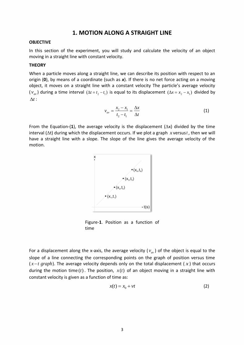
APPARATUS
Figure-2. The schematic representation of the experimental set-up with connection cables electrically connected to the air table.
5
PROCEDURE
1) Level the air table glass plate horizontally by using the adjustable legs.
2) Place the black carbon paper (50x50 cm) which is semiconducting on the glass plate. The carbon paper should be flat and on the air table given by the experimental set-up (Figure-2).
3) Place white recording paper as data sheet on the flat carbon paper.
4) Place two pucks on white paper. Keep one of the pucks stationary on a folded piece of data sheet at one corner of the air table.
5) For the alignment of the air table, adjust the legs of the air table so that the puck will come to rest about the center of the table.
6) Test both two switches for the compressor and spark timer operations. With the puck pedal, the single puck should move easily, almost without friction when compressor works. When the spark timer foot switch is pressed, black dots on white paper should be observed (on the side that faces the carbon paper).
7) Set the spark timer to Hzf 20 .
8) Now again, test the compressor only by pressing the puck footswitch. Make sure that the puck is moving freely on the air table. By activating both the puck pedal and spark timer pedal (foot switches) in the same time, test also the spark timer and observe the black dots on the recording paper.
9) Place the puck at the edge of the table then press both compressor and spark timer pedals as you push the puck on the surface of air table. It will move along the whole diagonal distance across the air table in a straight line with constant velocity. Then, stop the pedals.
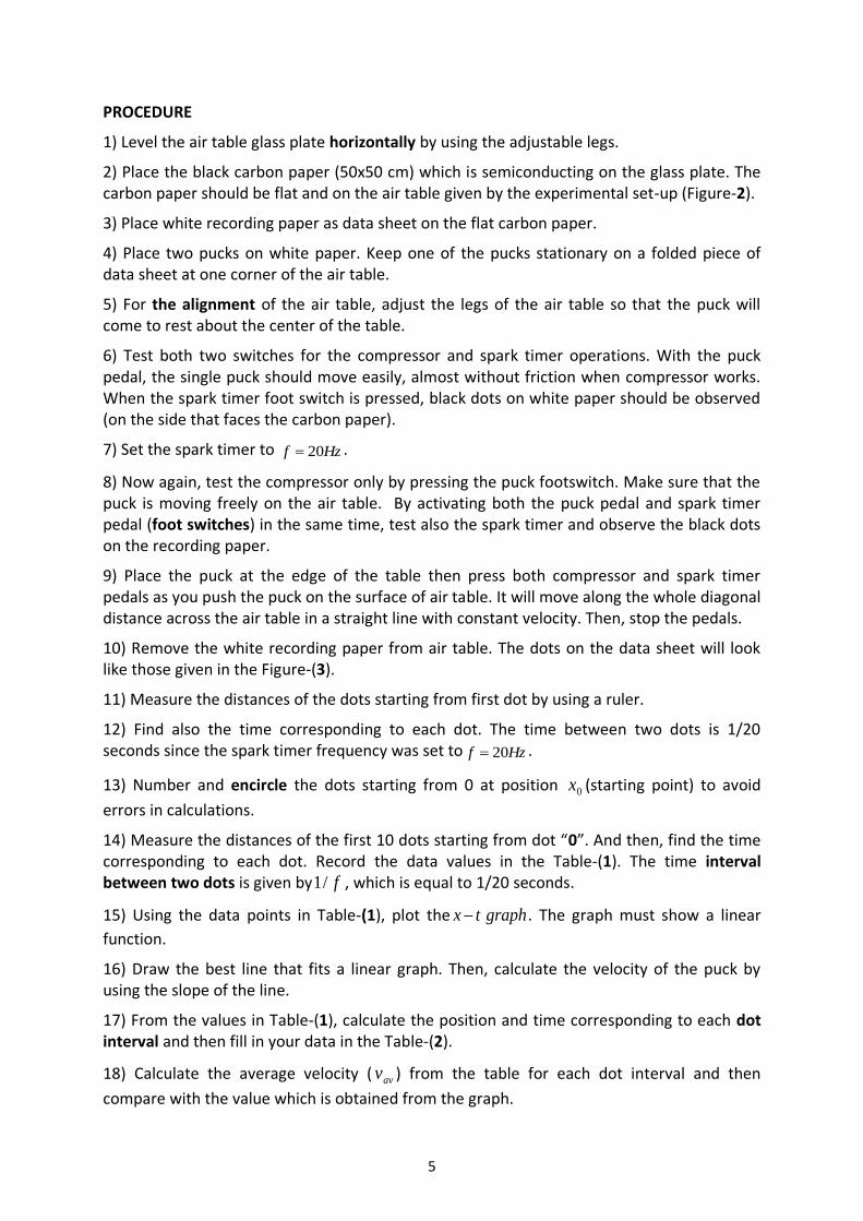
10) Remove the white recording paper from air table. The dots on the data sheet will look like those given in the Figure-(3).
11) Measure the distances of the dots starting from first dot by using a ruler.
12) Find also the time corresponding to each dot. The time between two dots is 1/20 seconds since the spark timer frequency was set to Hzf 20 .
13) Number and encircle the dots starting from 0 at position 0x (starting point) to avoid
errors in calculations.
14) Measure the distances of the first 10 dots starting from dot “0”. And then, find the time corresponding to each dot. Record the data values in the Table-(1). The time interval between two dots is given by f/1 , which is equal to 1/20 seconds.
15) Using the data points in Table-(1), plot the graphtx . The graph must show a linear
function.
16) Draw the best line that fits a linear graph. Then, calculate the velocity of the puck by using the slope of the line.
17) From the values in Table-(1), calculate the position and time corresponding to each dot interval and then fill in your data in the Table-(2).
18) Calculate the average velocity ( avv ) from the table for each dot interval and then
compare with the value which is obtained from the graph.
6
Figure-3. The dots produced by the puck on the data sheet.
LABARATORY REPORT
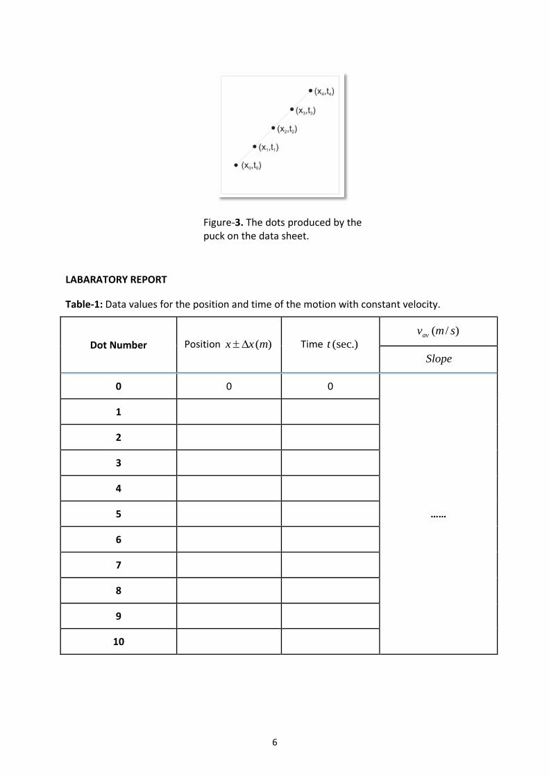
Table-1: Data values for the position and time of the motion with constant velocity.
Dot Number Position )(mxx Time .)(sect )/( smvav
Slope
0 0 0
……
1
2
3
4
5
6
7
8
9
10

7
QUESTIONS
1-Compare the average velocity found from the graph with the velocity calculated for the each time interval?
2-Discuss the difference in the velocity values calculated from the table and the values found from the graph. Is the difference approximately the same?
3-What are the sources of error in the experiment?
4-Write your comments related to the experiment.
Table-2: Experimental data values for the average velocity of the motion with constant velocity.
Interval Number
(n)
)(mxn )(1 mxn )(1 mxx nn .)(secnt )(1 stn )(1 stt nn )/( smv
0-1 0 0 0 0 0
1-2
2-3
3-4
4-5
5-6
6-7
7-8
8-9
9-10
(Note that nx is the position of the thn data point corresponding to the related dot).
8
2. PROJECTILE MOTION
OBJECTIVE
To study the fundamentals of projectile motion.
THEORY
The other type of the motion in this experiment is the horizontally projected motion. Projectile motion is the two-dimensional motion of an object under the influence of Earth’s gravitational acceleration, g . The path followed by a projectile is called its trajectory.
The position of such an object at any given time t is given by a set of coordinates x and y
which vary with respect to time and represent the horizontal and vertical coordinates, respectively. One of the two components of the velocity vector is parallel to the horizontal x-axis and the other is parallel to the vertical, or y-axis:
jvivv yxˆˆ
(4)
The motion of the object in the horizontal x direction is a straight line motion with constant
velocity. So, the x -component of the velocity )( xv will be constant.
However, the acceleration only acts along the vertical direction. The x -component of acceleration is zero and y -component is constant. This means that only the vertical
component of the velocity )( yv will change with respect to time and the horizontal
component of the velocity will be constant. Therefore, we can analyze projectile (two-dimensional) motion as a combination of horizontal motion with constant velocity and the vertical motion with constant acceleration.
We can express the vector relationships for the projectile’s acceleration by separate equations for the horizontal and vertical components. The components of the acceleration vector a
are:
0xa (5)
aa y (Constant) (6)
In vector form, the acceleration can be expressed as the form:
jaa yˆ
(7)
The position of the object at a given time is given by:
jyixr ˆˆ
(8)
For the two-dimensional ),( yx motion, we can separate acceleration )(a , displacement )(x
and velocity v in both x and y coordinate directions by the general equations below as:
2
002
1tatvxx xx (9)
2
002
1tatvyy yy (10)
9
In order to model two-dimensional projectile motion, a metal puck will be set in motion on an air table. When the air compressor is switched on, the air is supplied to down the tube under the puck so that it moves with a given initial velocity on the frictionless plane.
Suppose that at time 0t , the particle is at the point ),( 00 yx and at this time its velocity
components have the initial xv0 andyv0. Since the velocity of horizontal motion in the
projectile motion is constant, we find:
0xa (11)
xx vv 0 (12)
tvxx x 0 (13)
If we take the initial position )0( tat as the origin, then:
000 yx (14)
Using this relationship in the Equation-(13), we will find the equation of motion along the
axisx as:
tvx x (15)
For the motion along the axisy , the velocity )( yv at the later time, t becomes:
atv y (16)
2
2
1aty (17)
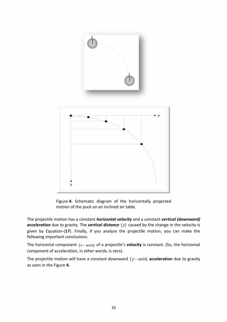
The dots produced on the data sheet will look like the figure as shown in the Figure-(4). Here, note that the intervals between the dots of the x -projections in the horizontal direction are equal.
10
The projectile motion has a constant horizontal velocity and a constant vertical (downward) acceleration due to gravity. The vertical distance )(y caused by the change in the velocity is
given by Equation-(17). Finally, if you analyze the projectile motion, you can make the following important conclusions:
The horizontal component )( axisx of a projectile’s velocity is constant. (So, the horizontal
component of acceleration, in other words, is zero).
The projectile motion will have a constant downward )( axisy acceleration due to gravity
as seen in the Figure 4.
Figure-4. Schematic diagram of the horizontally projected motion of the puck on an inclined air table.

11
APPARATUS
Figure-5. The schematic representation of the experimental set-up with connection cables electrically connected to the air table.
12
PROCEDURE
1) Place the foot leveling block at the upper leg of the air table to give the plane an inclination angle of 09 .
2) Adjust the frequency of the spark timer, Hzf 20 .
3) Keep one of the pucks stationary on a folded piece of data sheet paper and carbon paper at the lower corner of the plane.
4) Attach the shooter to the upper left side of the table with 00 (zero degrees) shooting angle to give horizontal shooting.
5) Make test shootings to find the best tension of the rubber to give a convenient trajectory.
6) First activate the compressor pedal and as you release the puck from the shooter also start the spark timer by pressing its pedal. Stop pressing both pedals when pucks reach the bottom of the plane. These dots are the data points of the trajectory- A .
7) Now, place the puck opposite to the shooter without tension of shooter (note that the puck must be outside the shooter). Then activate both compressor pedal and spark timer pedal in the same time and then let it slide freely down on the inclined plane. The dots will give trajectory- A .
8) Remove the data sheet and examine the dots of trajectory. You must get the trajectories illustrated in Figure-(6). If the data points are inconvenient to analyze, repeat the experiment and get new data.
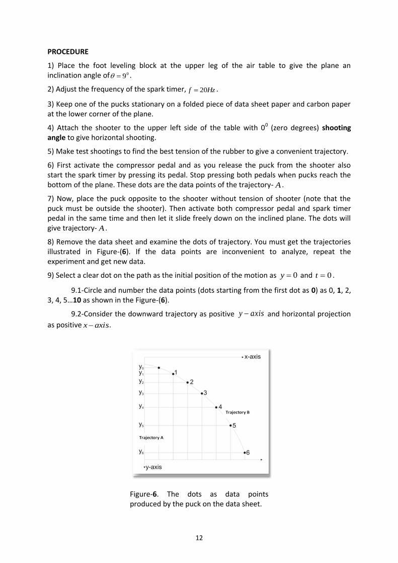
9) Select a clear dot on the path as the initial position of the motion as 0y and 0t .
9.1-Circle and number the data points (dots starting from the first dot as 0) as 0, 1, 2, 3, 4, 5…10 as shown in the Figure-(6).
9.2-Consider the downward trajectory as positive axisy and horizontal projection
as positive axisx .
Figure-6. The dots as data points produced by the puck on the data sheet.

13
10) Draw perpendicular lines from dots to axisyandx for the trajectory- B by taking the
first dot (dot 0) as the origin )0,0( . This origin is the initial position of
11) Measure the horizontal )(mx and vertical )(my displacements from the initial position
)0,0( and then record in the experimental data tables.
12) Determine the time )(t for each of these dots. The time interval between two dots is
given by f/1 , which is equal to 1/20 seconds. Then, calculate total time of flight )( ft
corresponding to the total horizontal displacement )( Rx of a projectile.
13) Calculate and record the horizontal velocity )( xv by using the time of flight )( ft and the
total horizontal distance traveled during the motion )( Rx . Complete the data Table-(3).
14) Starting from dot “0” of the trajectory-B, measure the distances of the y projections (y-
axis) of the first 10 data points (dots). Determine also the times corresponding to each of these dots.
14.1) Fill the measurements in the trajectory-B columns in the experimental data Table-(4).
15) Similarly, by starting from dot “0” of the trajectory-A, measure the distances of the y -
projections of the first 10 data points (dots).
15.1) Calculate the times corresponding to each of the dots for trajectory-A.
15.2) Record your data values in the trajectory-A columns in the Table-(4).
14
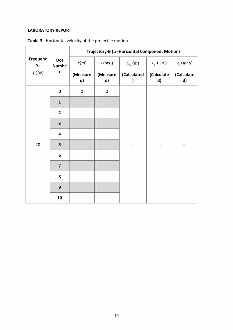
LABORATORY REPORT
Table-3: Horizontal velocity of the projectile motion.
Frequency,
)(Hzf
Dot Numbe
r
Trajectory-B ( x -Horizontal Component Motion)
)(mx (sec)t )(mxR (sec)ft )/( smvx
(Measured)
(Measured)
(Calculated)
(Calculated)
(Calculated)
20
0 0 0
….. ….. …..
1
2
3
4
5
6
7
8
9
10
15
QUESTIONS
Path 1 (straight line-trajectory-A):
Is the acceleration constant for the motion along the axis?
Path 2 (curved line- trajectory-B):
Is the horizontal velocity of a projected puck constant? Use your graph and data sheet for your explanation.
What is the horizontal acceleration of a projected puck?. Does the vertical velocity of the object increase downward in each time interval?. Is the vertical acceleration of projectile (two-dimensional) motion constant?.
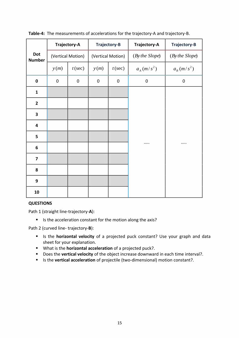
Table-4: The measurements of accelerations for the trajectory-A and trajectory-B.
Dot Number
Trajectory-A Trajectory-B Trajectory-A Trajectory-B
(Vertical Motion) (Vertical Motion) )( SlopetheBy )( SlopetheBy
)(my (sec)t )(my (sec)t )/( 2smaA )/( 2smaB
0 0 0 0 0 0 0
1
….. …..
2
3
4
5
6
7
8
9
10
16
3-HOOKE’S LAW
OBJECTIVE:
1. Investigate the behavior of the spring when a force is exerted on it and prove this
action as it completely explains the Hooke’s Law.
2. Examine the simple harmonic motion.
THEORY:
Hooke’s Law:
An ideal spring is a system which depends on how much the spring is streched as a result of
the force produced. This behavior of the spring is known as the ‘Hooke’s Law’. According to
Hooke’s Law, we need a force ( xkF ) that allows the spring streches more then its
original length as x . Here, k is the spring constant and this has different values for each
spring. Therefore, you should indicate the proportionality between the force exerted on the
spring (F) and the streching distance ( x ) and also show this proportion as a constant value.
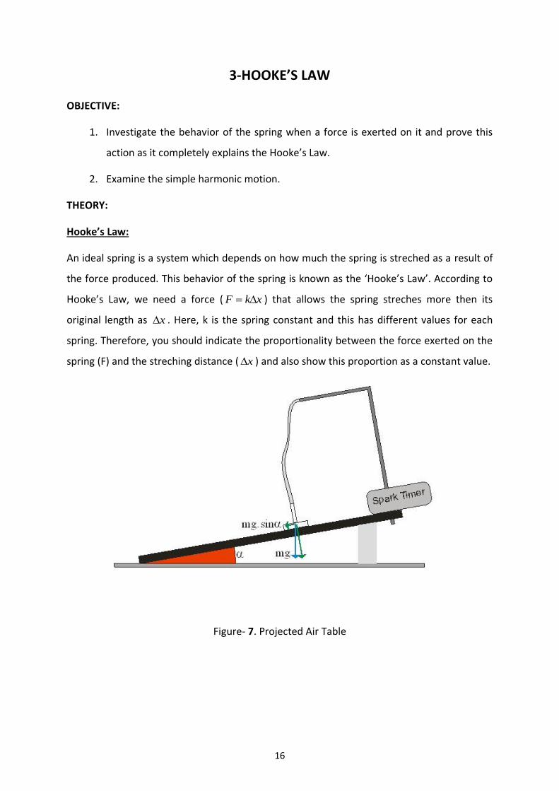
Figure- 7. Projected Air Table
17
In our experiment, first of all we levitate the air table to an inclined position.Then we
attach one of the disks to the spring to constitute the force that allows the spring elongates.
As a result of this, the gravitational force that stretches the spring downwards ( mgFg ) is
the parallel component ( sinmgFg ) of this force as illustrated in Figure 7.In Figure 8,as
demonstrated on air table, the force originated from the gravitational force is downwards,
the force exerted on the disc because of the spring is upwards. The spring can stretch until
the two forces are equal to each other.
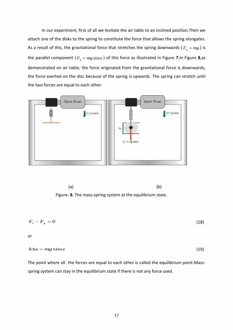
(a) (b)
Figure- 8. The mass-spring system at the equilibrium state.
0 gs FF (18)
or
sinmgxk (19)
The point where all the forces are equal to each other is called the equilibrium point.Mass-
spring system can stay in the equilibrium state if there is not any force used.
18
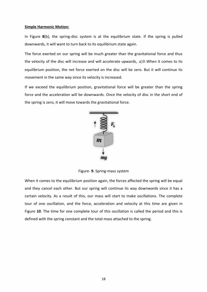
Simple Harmonic Motion:
In Figure 8(b), the spring-disc system is at the equilibrium state. If the spring is pulled
downwards, it will want to turn back to its equilibrium state again.
The force exerted on our spring will be much greater than the gravitational force and thus
the velocity of the disc will increase and will accelerate upwards, 0a .When it comes to its
equilibrium position, the net force exerted on the disc will be zero. But it will continue its
movement in the same way since its velocity is increased.
If we exceed the equilibrium position, gravitational force will be greater than the spring
force and the acceleration will be downwards. Once the velocity of disc in the short end of
the spring is zero, it will move towards the gravitational force.
Figure- 9. Spring-mass system
When it comes to the equilibrium position again, the forces affected the spring will be equal
and they cancel each other. But our spring will continue its way downwards since it has a
certain velocity. As a result of this, our mass will start to make oscillations. The complete
tour of one oscillation, and the force, acceleration and velocity at this time are given in
Figure 10. The time for one complete tour of this oscillation is called the period and this is
defined with the spring constant and the total mass attached to the spring.
19
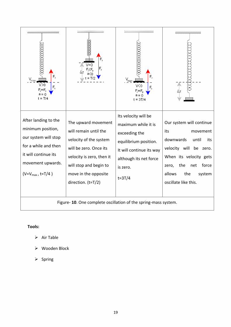
After landing to the
minimum position,
our system will stop
for a while and then
it will continue its
movement upwards.
(V=Vmax , t=T/4 )
The upward movement
will remain until the
velocity of the system
will be zero. Once its
velocity is zero, then it
will stop and begin to
move in the opposite
direction. (t=T/2)
Its velocity will be
maximum while it is
exceeding the
equilibrium position.
It will continue its way
although its net force
is zero.
t=3T/4
Our system will continue
its movement
downwards until its
velocity will be zero.
When its velocity gets
zero, the net force
allows the system
oscillate like this.
Figure- 10. One complete oscillation of the spring-mass system.
Tools:
Air Table
Wooden Block
Spring
20
PROCEDURE
1. Hooke Law
1. Get the air table to the inclined position using wood block.
2. To construct the mass-string system fix the spring to the higher corner of the air table by
using spring holder and mark the bottom point of the spring on the paper.
3. Tie one of the discs to the bottom of the spring.
4. Wait until the system gets into the equilibrium state and then mark it to the paper.
5. Add extra weight to the disc. Repeat step 4.
6.Draw xFg graph. Your graph has to be a straight line. Slope of this graph gives us the
spring constant(k) of that spring.
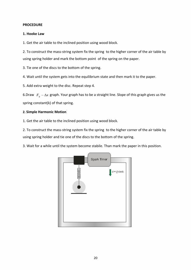
2. Simple Harmonic Motion
1. Get the air table to the inclined position using wood block.
2. To construct the mass-string system fix the spring to the higher corner of the air table by
using spring holder and tie one of the discs to the bottom of the spring.
3. Wait for a while until the system become stabile. Than mark the paper in this position.
21
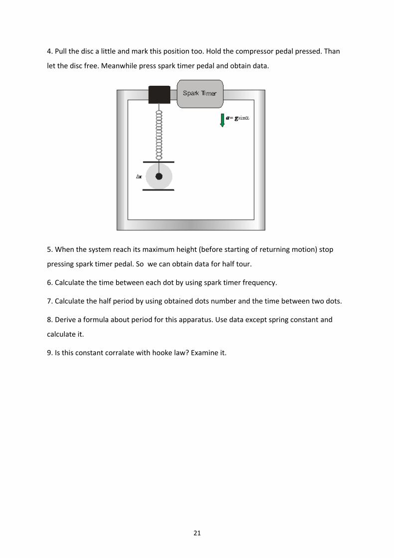
4. Pull the disc a little and mark this position too. Hold the compressor pedal pressed. Than
let the disc free. Meanwhile press spark timer pedal and obtain data.
5. When the system reach its maximum height (before starting of returning motion) stop
pressing spark timer pedal. So we can obtain data for half tour.
6. Calculate the time between each dot by using spark timer frequency.
7. Calculate the half period by using obtained dots number and the time between two dots.
8. Derive a formula about period for this apparatus. Use data except spring constant and
calculate it.
9. Is this constant corralate with hooke law? Examine it.
22
LABORATORY REPORT
xFg graph

23
4- CONSERVATION OF LINEAR MOMENTUM
OBJECTIVE
To study the principles of conservatıon of linear momentum.
THEORY
If we consider a particle of constant mass, m , we can write Newton’s second law for this particle as:
)( vmdt
d
dt
vdmF
(20)
Thus, Newton’s second law says that the net force acting on a particle equals to the time rate change of the combination, vm
(the product of the particle’s mass and velocity). This
combination is called as the momentum or linear momentum of the particle. Using the symbol p
for the momentum, we get the definition of the momentum:
vmp
(21)
If we substitute the definition of momentum into the Equation-(20), we get Newton’s second law in terms of momentum:
dt
(22)
According to Equation-(22), the net force (vector sum of all the forces) acting on a particle equals to the time rate change of the particle’s momentum. Since momentum is a vector quantity with the same direction as the particle’s velocity, we must express the momentum of a particle in terms of its components.
If the particle has the velocity components of ),( yx vv , then its momentum components will
be ),( yx pp . Then, the components of momentum are given by:
xx mvp (23)
yy mvp (24)
If there are no external forces (the net external force on a system is zero), the total
momentum of the system, P
(the vector sum of the momentum of the individual particles that make up the system) is constant or conserved. Each components of the total momentum is separately conserved. Remember that in any collision in which external forces can be neglected, momentum is conserved and the total momentum before equals to the total momentum after. Only in elastic collisions, the total kinetic energy before equals to the total the kinetic energy after. So, in an elastic collision between two bodies, the initial and final relative velocities have the same magnitude.
For a system with the two pucks, the total momentum )( tP before the collision will be the
same as the total momentum after the collision if the friction can be ignored.
By denoting initial momentums by the subscript ""i and final momentums by the "" f , the
vector equation for the principle of the conservation of momentum is given by:
24
ftit PP ,,
(25)
ffii PPPP ,2,1,2,1
(26)
Let the velocities of the two pucks be denoted iv ,1 and
iv ,2 before the collision as the initial
values and let the velocities after the collision be fv ,1and
fv ,2 as the final values.
Then, the magnitude of the momentum of the each puck before and after the collision will be:
ii mvP ,1,1 (27)
ii mvP ,2,2 (28)
ff mvP ,1,1 (29)
ff mvP ,2,2 (30)
In the any experiment, if we analyze the initial and final velocities of a system with the two particles (puck- A and B ), we get:
ffii vmvmvmvm ,22,11,22,11
(31)
where,
iv ,1: The velocity of puck- Abefore collision,
iv ,2: The velocity of puck- B before collision,
fv ,1: Final velocity of puck- A after collision,
fv ,2: Final velocity of puck- B after collision.
When the masses of the two pucks are equal )( 21 mmm , conservation of the momentum
gives the velocity vector relationship:
ffii vvvv ,2,1,2,1
(32)
Equations-(31) and (32) explain that the magnitude of the momentum will remain the same. The directions and velocities of the individual pucks may change, but vector sum )( ,2,1 ii vv
of their momentums will remain constant (total momentum is conserved).
Since the time interval )( t is constant between the successive dots on the data sheet
produced by each puck, the distance between two adjacent points on the trajectory of a puck will be proportional to the velocity ( v ). So, in a given experiment, the task of measuring the velocities of the two pucks reduces to that of measuring distances )(x of the dots.
25
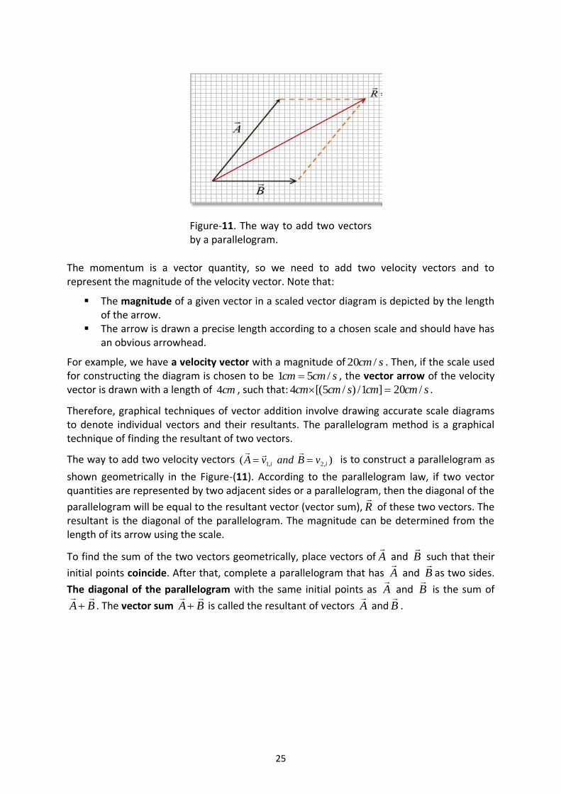
The momentum is a vector quantity, so we need to add two velocity vectors and to represent the magnitude of the velocity vector. Note that:
The magnitude of a given vector in a scaled vector diagram is depicted by the length of the arrow.
The arrow is drawn a precise length according to a chosen scale and should have has an obvious arrowhead.
For example, we have a velocity vector with a magnitude of scm /20 . Then, if the scale used for constructing the diagram is chosen to be scmcm /51 , the vector arrow of the velocity vector is drawn with a length of cm4 , such that: scmcmscmcm /20]1/)/5[(4 .
Therefore, graphical techniques of vector addition involve drawing accurate scale diagrams to denote individual vectors and their resultants. The parallelogram method is a graphical technique of finding the resultant of two vectors.
The way to add two velocity vectors )( ,2,1 ii vBandvA
is to construct a parallelogram as
shown geometrically in the Figure-(11). According to the parallelogram law, if two vector quantities are represented by two adjacent sides or a parallelogram, then the diagonal of the
parallelogram will be equal to the resultant vector (vector sum), R
of these two vectors. The resultant is the diagonal of the parallelogram. The magnitude can be determined from the length of its arrow using the scale.
To find the sum of the two vectors geometrically, place vectors of A
and B
such that their
initial points coincide. After that, complete a parallelogram that has A
and B
as two sides.
The diagonal of the parallelogram with the same initial points as A
and B
is the sum of
BA
. The vector sum BA
is called the resultant of vectors A
and B
.
Figure-11. The way to add two vectors by a parallelogram.
26
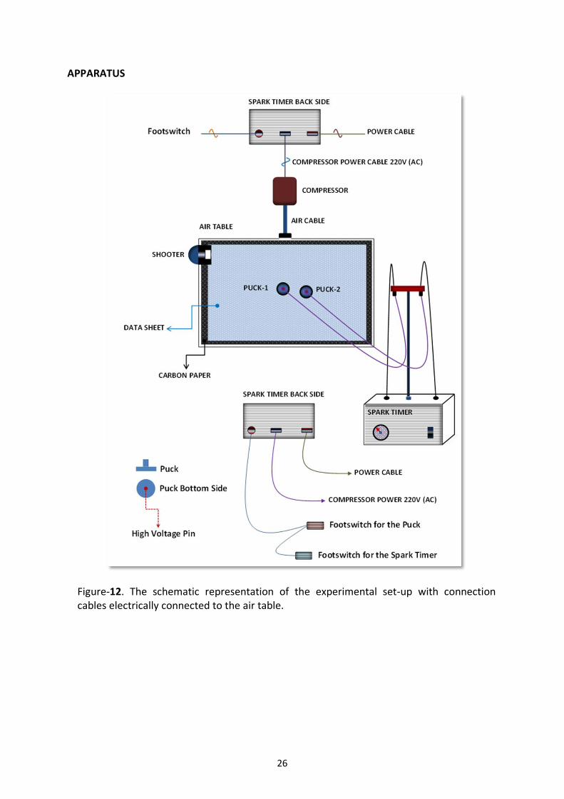
APPARATUS
Figure-12. The schematic representation of the experimental set-up with connection cables electrically connected to the air table.
27
PROCEDURE
This experiment will be carried on a level air table. We will investigate the conservation of momentum for two pucks moving on frictionless horizontal air table and we will assume there is no net external force on the system. The two pucks will be allowed to collide and then their total momentum before and after the collision will be measured.
1) By adjusting the legs of the air table, make sure it is precisely leveled.
2) Choose the spark timer frequency as Hzf 20 .
3) Activate the compressor and spark timer switches in the same time, and then push the two pucks diagonally to get a collision nearly at the center of the table. Don’t push too slowly or too fast, you will find the best speed after several experimental test observations.
4) Release the two switches when they complete their motion after the collision.
5) Remove the data sheet on the air table.
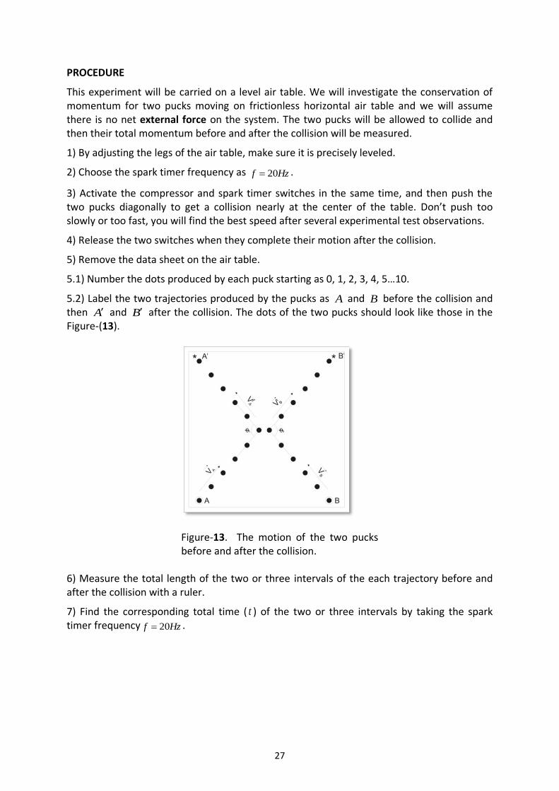
5.1) Number the dots produced by each puck starting as 0, 1, 2, 3, 4, 5…10.
5.2) Label the two trajectories produced by the pucks as A and B before the collision and then A and B after the collision. The dots of the two pucks should look like those in the Figure-(13).
6) Measure the total length of the two or three intervals of the each trajectory before and after the collision with a ruler.
7) Find the corresponding total time ( t ) of the two or three intervals by taking the spark timer frequency Hzf 20 .
Figure-13. The motion of the two pucks before and after the collision.
28
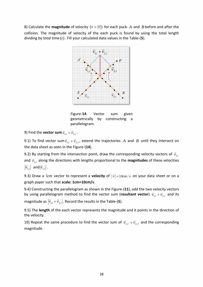
8) Calculate the magnitude of velocity )( vv
for each puck- A and B before and after the
collision. The magnitude of velocity of the each puck is found by using the total length dividing by total time )(t . Fill your calculated data values in the Table-(5).
9) Find the vector sumii vv ,2,1
.
9.1) To find vector sumii vv ,2,1
, extend the trajectories A and B until they intersect on
the data sheet as seen in the Figure-(14).
9.2) By starting from the intersection point, draw the corresponding velocity vectors of iv ,1
and iv ,2
along the directions with lengths proportional to the magnitudes of these velocities
iv ,1
and iv ,2
.
9.3) Draw a cm1 vector to represent a velocity of scmv /10ˆ on your data sheet or on a
graph paper such that scale: 1cm=10cm/s.
9.4) Constructing the parallelogram as shown in the Figure-(11), add the two velocity vectors by using parallelogram method to find the vector sum (resultant vector)
ii vv ,2,1
and its
magnitude as ii vv ,2,1
. Record the results in the Table-(5).
9.5) The length of the each vector represents the magnitude and it points in the direction of the velocity.
10) Repeat the same procedure to find the vector sum of ff vv ,2,1
and the corresponding
magnitude.
Figure-14. Vector sum given geometrically by constructing a parallelogram.
29
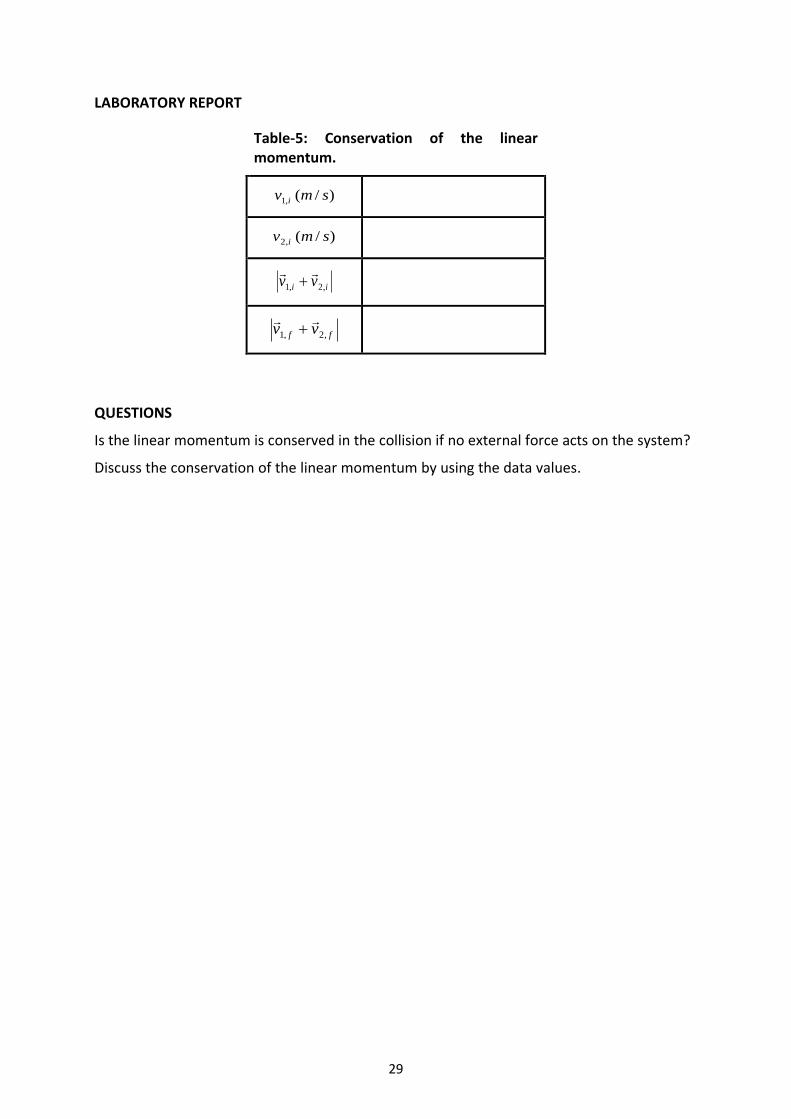
LABORATORY REPORT
QUESTIONS
Is the linear momentum is conserved in the collision if no external force acts on the system?
Discuss the conservation of the linear momentum by using the data values.
Table-5: Conservation of the linear momentum.
)/(,1 smv i
)/(,2 smv i
ii vv ,2,1
ff vv ,2,1
30
5. ROTATIONAL MOTION
OBJECTIVE
1. Investigating dynamics of a rotating disc 2. Investigating 'conservation of angular momentum and mechanical energy' 3. Finding the value 'moment of inertia of a rotating disc'
THEORY
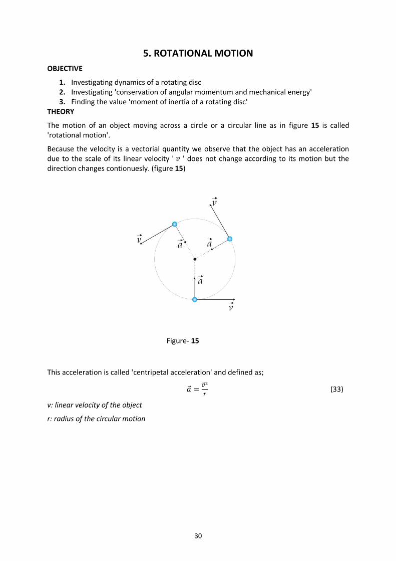
The motion of an object moving across a circle or a circular line as in figure 15 is called 'rotational motion'.
Because the velocity is a vectorial quantity we observe that the object has an acceleration due to the scale of its linear velocity ' ' does not change according to its motion but the direction changes contionuesly. (figure 15)
Figure- 15
This acceleration is called 'centripetal acceleration' and defined as;
(33)
v: linear velocity of the object
r: radius of the circular motion

31
Figure- 16
The linear velocity and centripetal acceleration of the object 'p' is shown in Figure 16.
In equation
(34)
we have ve , so we can define
(
) (
) (35)
With the derivation of velocity equation, acceleration of the object will be;
(
) (
) (36)
In equation (36)
and
so we get equation (35);
(
) (
) (37)
Figure 16.b gives us the components of the acceleration vector as ; √
√
√
(38)
and
, then ;
( ⁄ )
( ⁄ ) (39)
In equation (39) . This means the direction of the acceleration of the object is into the center of the circular path.
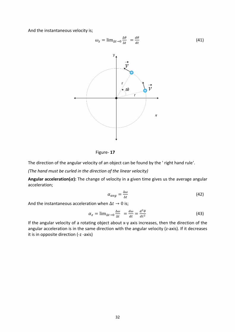
Angular velocity (ω): Average angular velocity of a rotating object as shown in Figure 17 is defined as;
(40)
32
And the instantaneous velocity is;
(41)
Figure- 17
The direction of the angular velocity of an object can be found by the ' right hand rule'.
(The hand must be curled in the direction of the linear velocity)
Angular acceleration( ): The change of velocity in a given time gives us the average angular acceleration;
(42)
And the instantaneous acceleration when is;
(43)
If the angular velocity of a rotating object about x-y axis increases, then the direction of the angular acceleration is in the same direction with the angular velocity (z-axis). If it decreases it is in opposite direction (-z -axis)
33
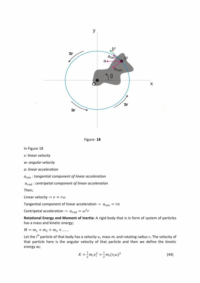
Figure- 18
In Figure 18
v: linear velocity
w: angular velocity
a: linear acceleration
: tangential component of linear acceleration
: centripetal component of linear acceleration
Then;
Linear velocity
Tangential component of linear acceleration
Centripetal acceleration
Rotational Energy and Moment of Inertia: A rigid body that is in form of system of particles has a mass and kinetic energy;
.......
Let the ith particle of that body has a velocity vi, mass mi and rotating radius ri. The velocity of that particle here is the angular velocity of that particle and then we define the kinetic energy as;
( )
(44)
34
then the total kinetic energy will be ;
∑
(45)
(
)
(∑
) (46)
The equation in parentheses describes 'the moment of inertia' and symbolized with 'I';
∑
(47)
The value of moment of inertia of an object depends of its shape and rotating axis.
∫ ∫ (48)
“ ”: density of the body
“ ”: volume element of the body
“r”: radius of the body
The rotational kinetic energy of a body or an object will be:
(49)
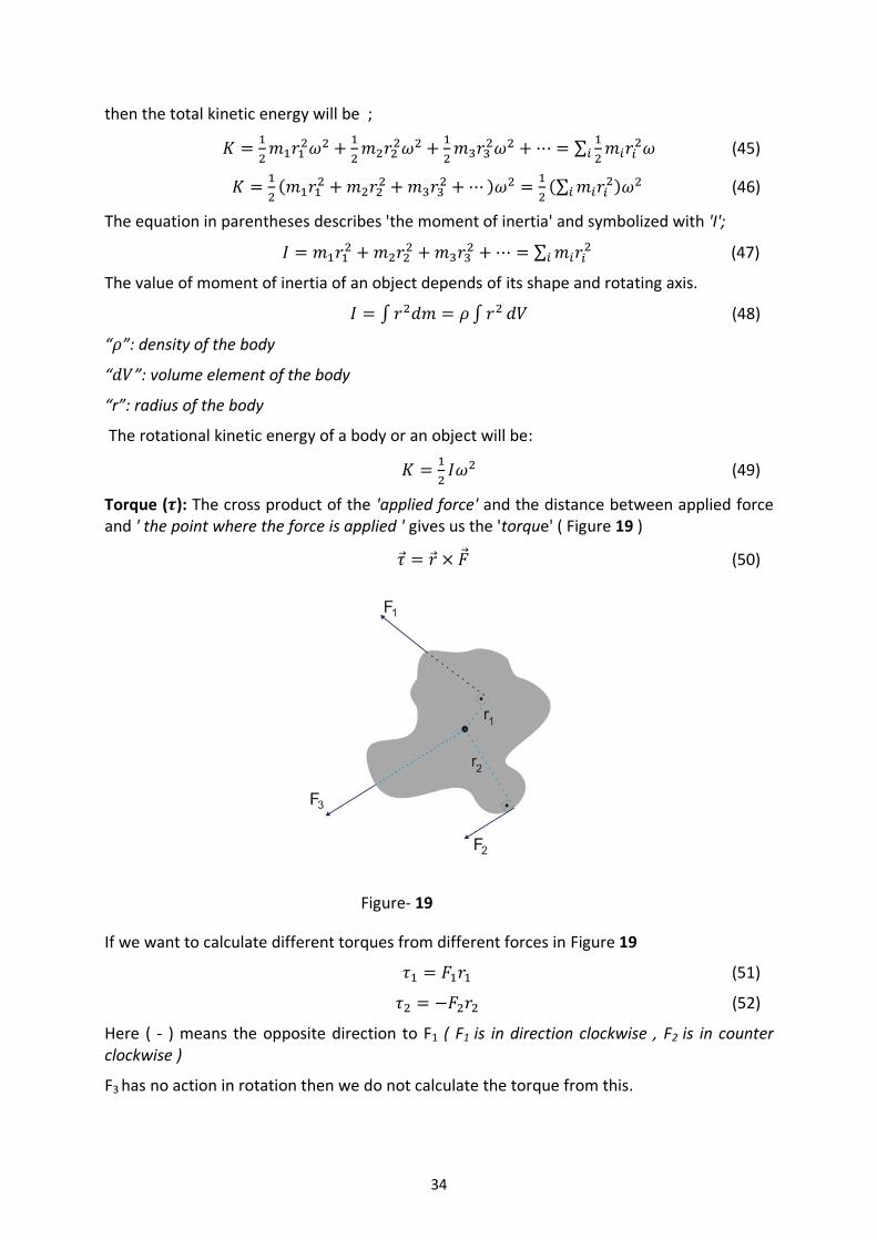
Torque ( ): The cross product of the 'applied force' and the distance between applied force and ' the point where the force is applied ' gives us the 'torque' ( Figure 19 )
(50)
Figure- 19
If we want to calculate different torques from different forces in Figure 19
(51)
(52)
Here ( - ) means the opposite direction to F1 ( F1 is in direction clockwise , F2 is in counter clockwise )
F3 has no action in rotation then we do not calculate the torque from this.
35
Because the applied force to the body is tangential to the rotating axis we can describe the torque as;
( ) (53)
Here we will use angular acceleration instead of linear acceleration, then the equation (53) will be;
( ) (54)
This gives us the torque of ith particle and the total torque of the body will be;
∑ ∑ ( ) (55)
“∑
” describes the moment of inertia then the general formula of torque is
(56)
Angular Momentum (L): Angular momentum of an object is described as rotation of the linear momentum of that object relative to a point.
(57)
r: position vector that is relative to linear momentum vector with the rotating axis
P: linear position vector
The direction of 'L' vector can be found by 'the right hand rule'.
With the general equation of linear momentum we get;
( ) (58)
The change in angular momentum that is formed by an applied force is equal to the torque that is formed by that applied force.
(
) (
) ( ) ( ) (59)
Here the first term is equal to zero ( ), then ;
(60)
36
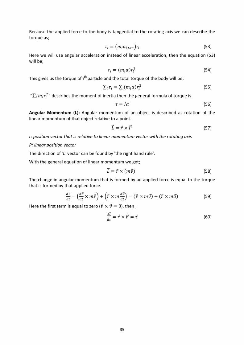
The angular momentum (equation 59) of ith particle of a rigid body in figure 20 is described as;
( ) (61)
So the total angular momentum of the whole body will be;
∑ (∑
) (62)
The expression with parentheses in equation 62 is the same with equation 47 and describes the moment of inertia, then equation 62 will be;
(63)
Figure- 20
37
APPARATUS
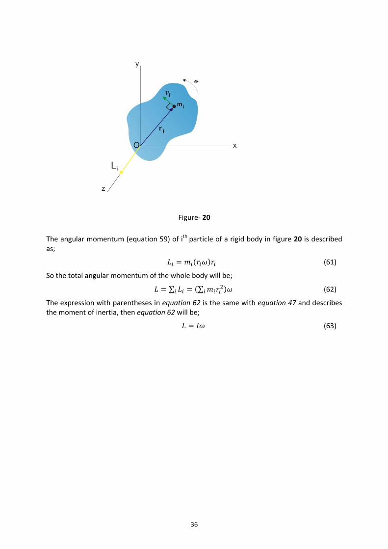
Figure-21. Top view of the experiment set
38
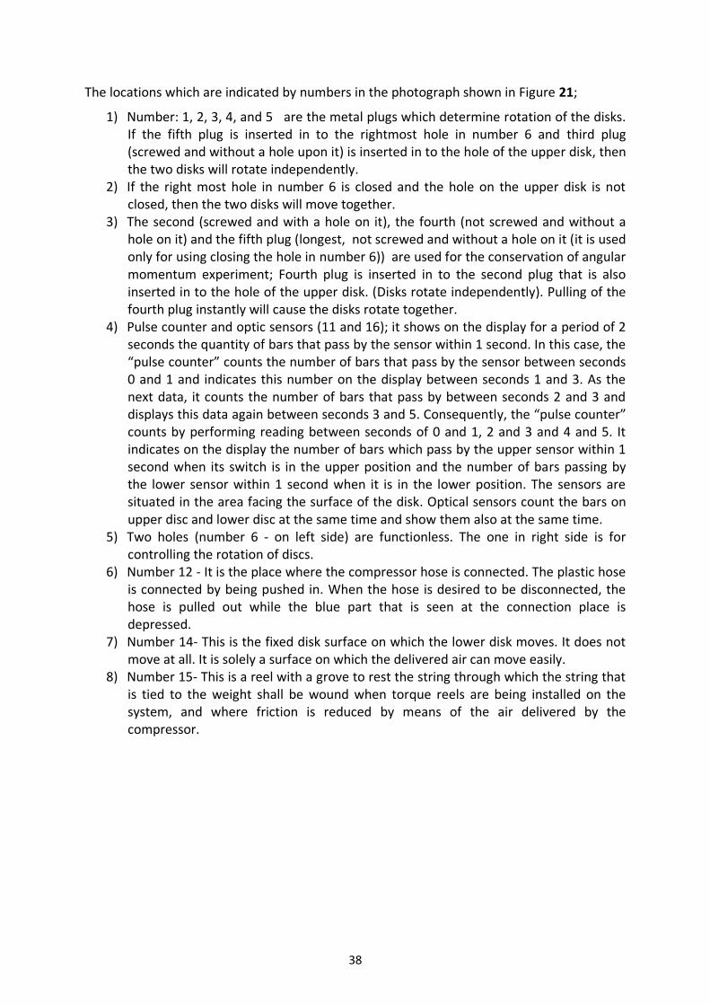
The locations which are indicated by numbers in the photograph shown in Figure 21;
1) Number: 1, 2, 3, 4, and 5 are the metal plugs which determine rotation of the disks. If the fifth plug is inserted in to the rightmost hole in number 6 and third plug (screwed and without a hole upon it) is inserted in to the hole of the upper disk, then the two disks will rotate independently.
2) If the right most hole in number 6 is closed and the hole on the upper disk is not closed, then the two disks will move together.
3) The second (screwed and with a hole on it), the fourth (not screwed and without a hole on it) and the fifth plug (longest, not screwed and without a hole on it (it is used only for using closing the hole in number 6)) are used for the conservation of angular momentum experiment; Fourth plug is inserted in to the second plug that is also inserted in to the hole of the upper disk. (Disks rotate independently). Pulling of the fourth plug instantly will cause the disks rotate together.
4) Pulse counter and optic sensors (11 and 16); it shows on the display for a period of 2 seconds the quantity of bars that pass by the sensor within 1 second. In this case, the “pulse counter” counts the number of bars that pass by the sensor between seconds 0 and 1 and indicates this number on the display between seconds 1 and 3. As the next data, it counts the number of bars that pass by between seconds 2 and 3 and displays this data again between seconds 3 and 5. Consequently, the “pulse counter” counts by performing reading between seconds of 0 and 1, 2 and 3 and 4 and 5. It indicates on the display the number of bars which pass by the upper sensor within 1 second when its switch is in the upper position and the number of bars passing by the lower sensor within 1 second when it is in the lower position. The sensors are situated in the area facing the surface of the disk. Optical sensors count the bars on upper disc and lower disc at the same time and show them also at the same time.
5) Two holes (number 6 - on left side) are functionless. The one in right side is for controlling the rotation of discs.
6) Number 12 - It is the place where the compressor hose is connected. The plastic hose is connected by being pushed in. When the hose is desired to be disconnected, the hose is pulled out while the blue part that is seen at the connection place is depressed.
7) Number 14- This is the fixed disk surface on which the lower disk moves. It does not move at all. It is solely a surface on which the delivered air can move easily.
8) Number 15- This is a reel with a grove to rest the string through which the string that is tied to the weight shall be wound when torque reels are being installed on the system, and where friction is reduced by means of the air delivered by the compressor.
39
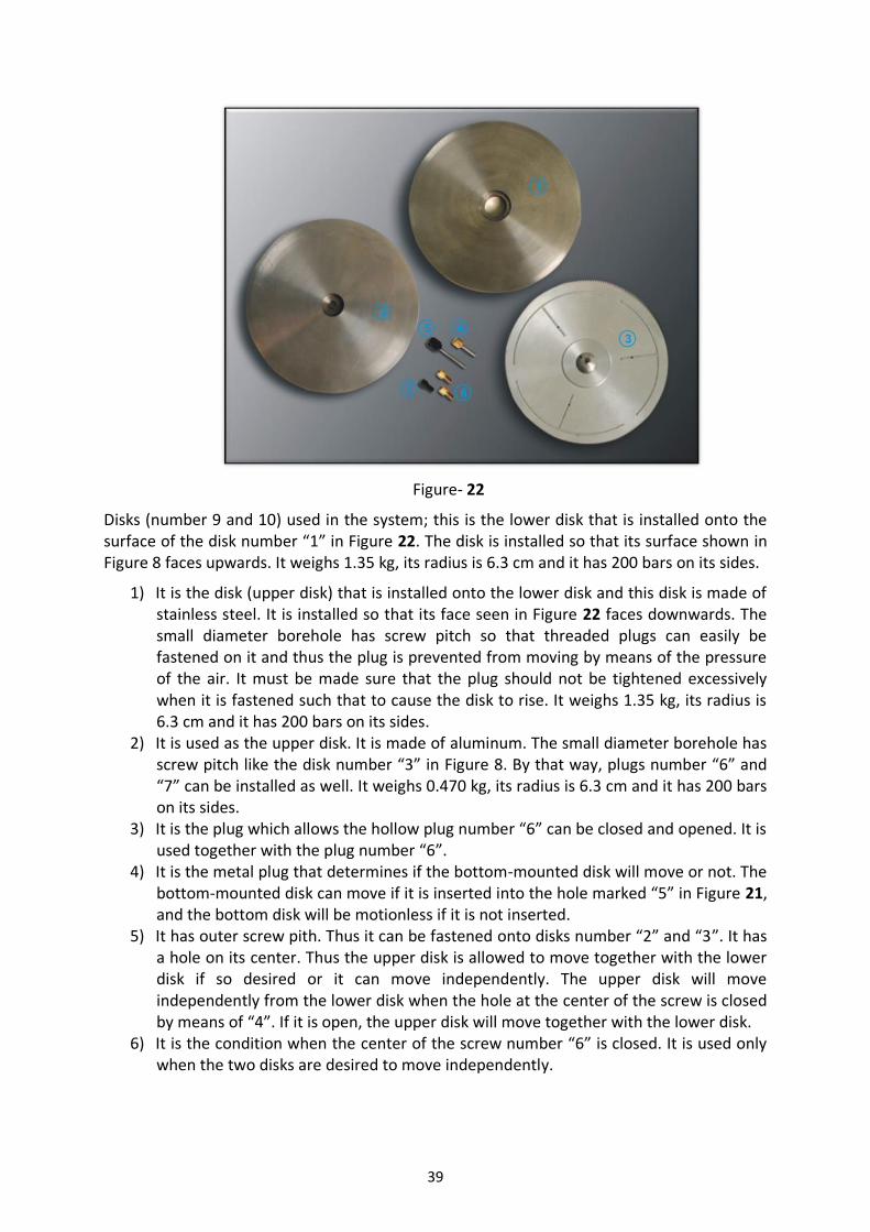
Figure- 22
Disks (number 9 and 10) used in the system; this is the lower disk that is installed onto the surface of the disk number “1” in Figure 22. The disk is installed so that its surface shown in Figure 8 faces upwards. It weighs 1.35 kg, its radius is 6.3 cm and it has 200 bars on its sides.
1) It is the disk (upper disk) that is installed onto the lower disk and this disk is made of stainless steel. It is installed so that its face seen in Figure 22 faces downwards. The small diameter borehole has screw pitch so that threaded plugs can easily be fastened on it and thus the plug is prevented from moving by means of the pressure of the air. It must be made sure that the plug should not be tightened excessively when it is fastened such that to cause the disk to rise. It weighs 1.35 kg, its radius is 6.3 cm and it has 200 bars on its sides.
2) It is used as the upper disk. It is made of aluminum. The small diameter borehole has screw pitch like the disk number “3” in Figure 8. By that way, plugs number “6” and “7” can be installed as well. It weighs 0.470 kg, its radius is 6.3 cm and it has 200 bars on its sides.
3) It is the plug which allows the hollow plug number “6” can be closed and opened. It is used together with the plug number “6”.
4) It is the metal plug that determines if the bottom-mounted disk will move or not. The bottom-mounted disk can move if it is inserted into the hole marked “5” in Figure 21, and the bottom disk will be motionless if it is not inserted.
5) It has outer screw pith. Thus it can be fastened onto disks number “2” and “3”. It has a hole on its center. Thus the upper disk is allowed to move together with the lower disk if so desired or it can move independently. The upper disk will move independently from the lower disk when the hole at the center of the screw is closed by means of “4”. If it is open, the upper disk will move together with the lower disk.
6) It is the condition when the center of the screw number “6” is closed. It is used only when the two disks are desired to move independently.
40
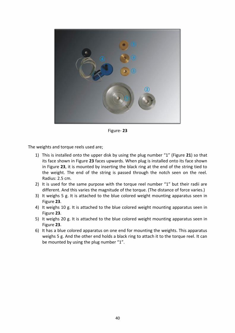
Figure- 23
The weights and torque reels used are;
1) This is installed onto the upper disk by using the plug number “1” (Figure 21) so that its face shown in Figure 23 faces upwards. When plug is installed onto its face shown in Figure 23, it is mounted by inserting the black ring at the end of the string tied to the weight. The end of the string is passed through the notch seen on the reel. Radius: 2.5 cm.
2) It is used for the same purpose with the torque reel number “1” but their radii are different. And this varies the magnitude of the torque. (The distance of force varies.)
3) It weighs 5 g. It is attached to the blue colored weight mounting apparatus seen in Figure 23.
4) It weighs 10 g. It is attached to the blue colored weight mounting apparatus seen in Figure 23.
5) It weighs 20 g. It is attached to the blue colored weight mounting apparatus seen in Figure 23.
6) It has a blue colored apparatus on one end for mounting the weights. This apparatus weighs 5 g. And the other end holds a black ring to attach it to the torque reel. It can be mounted by using the plug number “1”.
41
PROCEDURE
1-Measurement of Angular Velocity 1) Set up the system so that the lower disk is fixed and the upper disk is movable. 2) Set the “Pulse Counter” to the position where it reads the upper disk. 3) Operate the compressor. 4) Hold the upper disk stationary by your hand. Wait for the digital display indicate zero. 5) Make the upper disk rotate by applying force for only once by your hand. 6) Record the successively read data to Table 6. 7) The values you read are the numbers of the bars that pass by the sensor in 1 second ( ).
Calculate the angular velocity of the disk by using this information;
Value of Angle (Degrees) = (360/200) ß Value of Angle (Radians) = Value of Angle x 2π/360 We obtain the angular velocity when we divide this angle value by 1 second. w = Value of Angle (Radians) /1s When we write this solution in simple form, we obtain;
To Find the Rotational Moment of Inertia
1) Set up the system so that the lower disk is fixed and the upper disk is movable. 2) Set the “Pulse Counter” to the position where it reads the upper disk. 3) Attach to the upper disk the small radius torque reel and the ring on the end of the string which is tied to the weight. Pull the string out from the notch on the torque reel. 4) Pass the string of the weight through the notch on the reel and let it hang downwards. It must be made sure that the string does not make an angle between its exit from the torque reel and the reel. For that reason the torque reel must wind the string in right direction. 5) Attach the 10 g mass to the weight mounting apparatus. 6) Operate the compressor. 7) Raise the weight up to the reel by winding the string onto the torque reel. 8) Release the system free after observing that the digital display indicates zero. 9) Record the values read by the sensor to Table 7. 10) The values are read with intervals of 1 second. Take care of this. 11) Calculate the angular velocity for each data by using the read values. 12) Draw angular velocity versus time curve on millimeter paper. 13) The slope of the drawn curve gives us the angular acceleration. 14) Calculate the torque by using Equation (49). In this equation, force is the hanging weight and the force distance (r) is the radius of the torque reel. There is an angle of 90º between these two vectors.
42
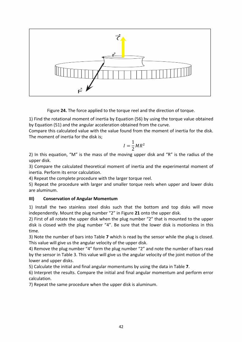
Figure 24. The force applied to the torque reel and the direction of torque.
1) Find the rotational moment of inertia by Equation (56) by using the torque value obtained by Equation (51) and the angular acceleration obtained from the curve. Compare this calculated value with the value found from the moment of inertia for the disk. The moment of inertia for the disk is;
2) In this equation, “M” is the mass of the moving upper disk and “R” is the radius of the upper disk. 3) Compare the calculated theoretical moment of inertia and the experimental moment of inertia. Perform its error calculation. 4) Repeat the complete procedure with the larger torque reel. 5) Repeat the procedure with larger and smaller torque reels when upper and lower disks are aluminum.
III) Conservation of Angular Momentum
1) Install the two stainless steel disks such that the bottom and top disks will move independently. Mount the plug number “2” in Figure 21 onto the upper disk. 2) First of all rotate the upper disk when the plug number “2” that is mounted to the upper disk is closed with the plug number “4”. Be sure that the lower disk is motionless in this time. 3) Note the number of bars into Table 7 which is read by the sensor while the plug is closed. This value will give us the angular velocity of the upper disk. 4) Remove the plug number “4” form the plug number “2” and note the number of bars read by the sensor in Table 3. This value will give us the angular velocity of the joint motion of the lower and upper disks. 5) Calculate the initial and final angular momentums by using the data in Table 7. 6) Interpret the results. Compare the initial and final angular momentum and perform error calculation. 7) Repeat the same procedure when the upper disk is aluminum.

43
IV) Calculation of Kinetic Energy and Potential Energy 1) Install the stainless steel disks so that the lower disk is fixed and the upper disk is movable. 2) Install the smaller radius torque reel and the weight pin onto the upper disk. 3) Attach the 10 g mass to the weight mounting apparatus. 4) Pass the weight string through the groove of the reel and leave its end free. 5) Wind the weight string onto the torque reel. 6) Wait until the digital display indicates “zero” and then release the upper disk. 7) Write down the number of bars read initially. 8) Show equality of energy from displacement of the weight in the vertical axis and from its speed at the end of 1 second. 9) The potential energy which the weight had at the beginning was;
(
)
Here, “r” is the radius of the torque reel.
Figure 25. Period of 1 second from start of motion of the upper disk and angular velocities.
The kinetic energy which the weight has at the end of 1 second is;
In this equation;
Here, is the angular velocity found from the number of bars read by the sensors in 1 second (Figure 25). And can be found from the equation of The moment
of inertia concerned here is the moment of inertia of the upper disk. It is calculated for the steel and aluminum disks in part II of the experiment. After these values are obtained, can easily be found.
In the above kinetic energy equation, , It should be noted that the radius used when calculating the linear speed is the radius of the torque reel.
9) The potential and the kinetic energy must be equal. Perform error calculation by comparing PE and KE.

44
10) Repeat the same procedure by using the larger radius torque reel and the aluminum upper disk.
LABORATORY REPORT
I) Measurement of Angular Velocity
TABLE 6
Number of Bars Read
Angular Velocity ( ⁄ )
45
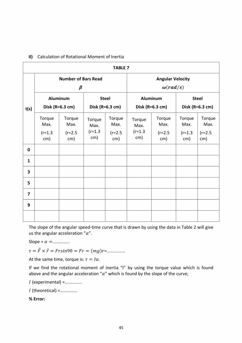
II) Calculation of Rotational Moment of Inertia
TABLE 7
t(s)
Number of Bars Read
Angular Velocity
( ⁄ )
Aluminum
Disk (R=6.3 cm)
Steel
Disk (R=6.3 cm)
Aluminum
Disk (R=6.3 cm)
Steel
Disk (R=6.3 cm)
Torque Max.
(r=1.3 cm)
Torque Max.
(r=2.5 cm)
Torque Max. (r=1.3 cm)
Torque Max.
(r=2.5 cm)
Torque Max. (r=1.3 cm)
Torque Max.
(r=2.5 cm)
Torque Max.
(r=1.3 cm)
Torque Max.
(r=2.5 cm)
0
1
3
5
7
9
The slope of the angular speed-time curve that is drawn by using the data in Table 2 will give us the angular acceleration “ ”.
Slope = ..............
( ) =...............
At the same time, torque is: .
If we find the rotational moment of inertia “I” by using the torque value which is found above and the angular acceleration “ ” which is found by the slope of the curve;
(experimental) =..............
(theoretical) =..............
% Error:
46
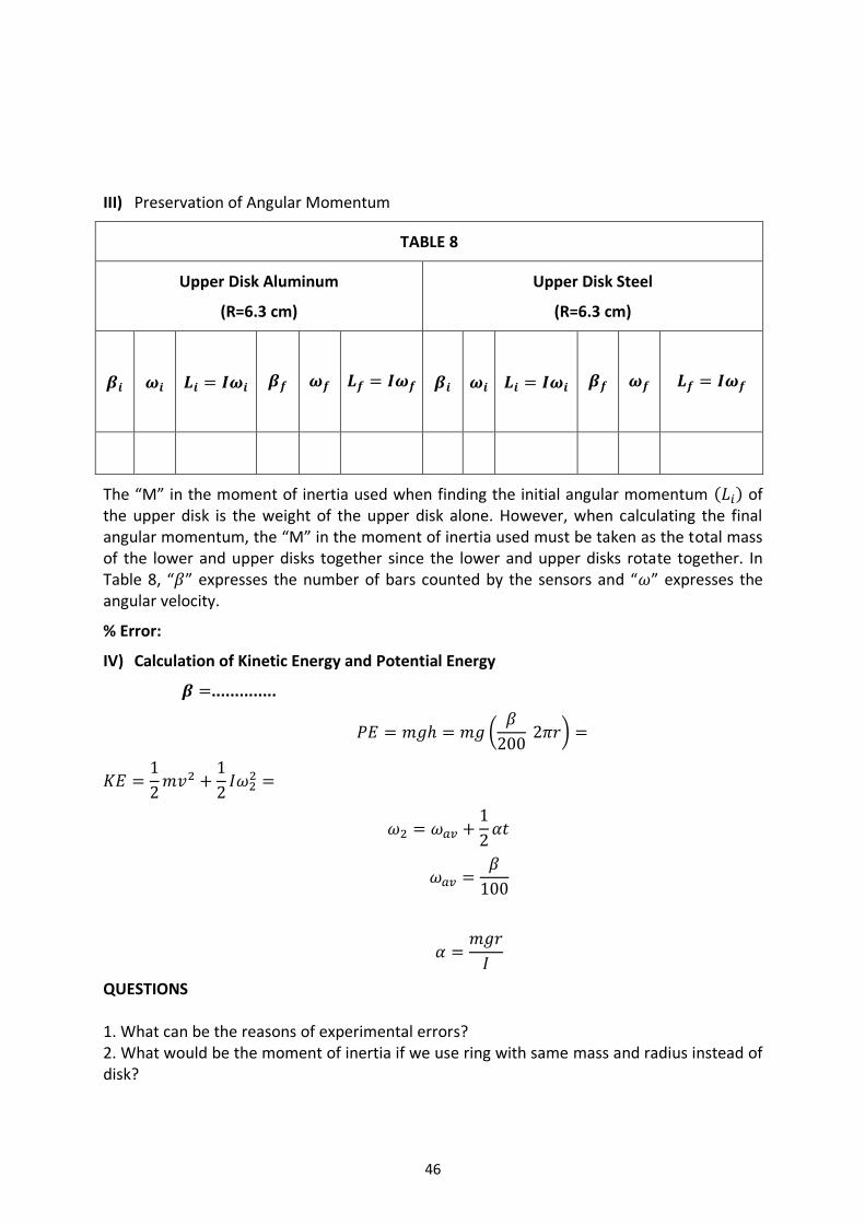
III) Preservation of Angular Momentum
TABLE 8
Upper Disk Aluminum
(R=6.3 cm)
Upper Disk Steel
(R=6.3 cm)
The “M” in the moment of inertia used when finding the initial angular momentum ( ) of the upper disk is the weight of the upper disk alone. However, when calculating the final angular momentum, the “M” in the moment of inertia used must be taken as the total mass of the lower and upper disks together since the lower and upper disks rotate together. In Table 8, “ ” expresses the number of bars counted by the sensors and “ ” expresses the angular velocity.
% Error:
IV) Calculation of Kinetic Energy and Potential Energy
..............
(
)
QUESTIONS 1. What can be the reasons of experimental errors? 2. What would be the moment of inertia if we use ring with same mass and radius instead of disk?
47
6.SIMPLE PENDULUM
OBJECTIVE
Measure the period of pendulum as a function of amptitude
Measure the period of pendulum as a function of length
Measure the period of pendulum as a function of bob mass
Observe and investigate the conservation of energy
THEORY
Frequency is the number of occurences of a repeating event per unit time. It is also referred to as temporal frequency. The period is the duration of one cycle in a repeating event, so the period is the reciprocal of the frequency.
Hence we can say;
(64)
Angular velocity (ω) is a scalar measure of rotational rate. Angular frequency is the magnitude of the vector quantity angular velocity
(65)
Above we can see that the speed of the pendulum is dependent on the period.
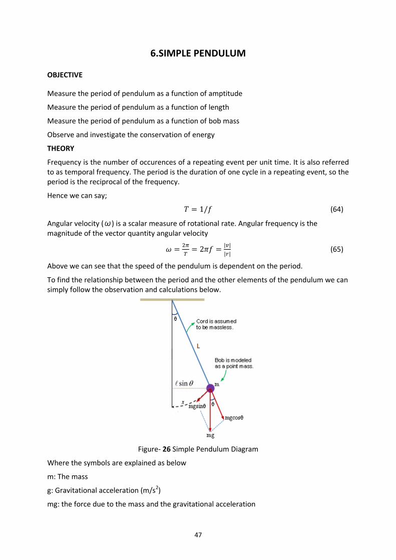
To find the relationship between the period and the other elements of the pendulum we can simply follow the observation and calculations below.
Figure- 26 Simple Pendulum Diagram
Where the symbols are explained as below
m: The mass
g: Gravitational acceleration (m/s2)
mg: the force due to the mass and the gravitational acceleration
48
L: the length of pendulum rod
Looking at the force vector one can derive the following equation:
(66)
For small angles (≤10o) an angle's sinus is equal to the angle:
(67)
Therefore one can see that the force, which affects the pendulum, will be
(68)
Also we can easily say where x is the change in position
(69)
Hence we can say
⁄ (70)
By using equations (70) and (68) we can derive that:
(71)
Here we can see that the force constant equals to
(72)
From here we can easily derive the following equation for simple harmonic motions
√
Simple harmonic motion (73)
By using equations (72) and (73) we can obtain:
√ ⁄
(74)
√
49
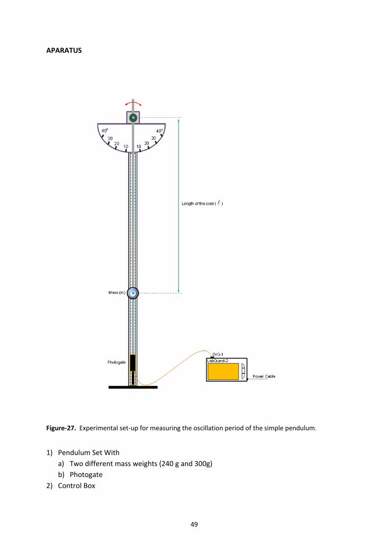
APARATUS
1) Pendulum Set With
a) Two different mass weights (240 g and 300g)
b) Photogate
2) Control Box
Figure-27. Experimental set-up for measuring the oscillation period of the simple pendulum.
50
PROCEDURE
1. By using the 240 g mass adjust the pendulum length to at least 65 cm.
2. By using the Spirit Level make sure the base of the pendulum is flat.
3. On the control box switch to mode 1.
4. Temporarily hold the mass out of the center of the Photogate. Observe the live readings on the screen. Block the Photogate with your hand. Note the time difference between blocked and unblocked.
5.Temporarily hold the mass out of the center of the Photogate. Start data collection to prepare the Photogate.
6. Now you can perform a trial measurement of the period of your pendulum. Hold the mass from about 10o from vertical and release. After five trails have been recorded, stop data collections.
7. Read the period.
8. When you ready measure another period,simply start data collection again. You will use this method for each period measurement below.
Part-1 Amplitude
9. Determine how the period depends on amplitudes. Use a range of amplitudes, from just barely enough to unblock the Photogate, to about 30o.Each time, measure the amplitude using the protractor so that the mass with the string is released at a known angle. Repeat this step for each different amplitude. Record the data in your table.
Part-2 Length
10. Use the method you learned above to investigate the effect of changing pendulum length on the period. Use the 240 g mass and consistent amplitude of 10o for each trial. Vary the pendulum length in steps of 10 cm, from 65 cm to 50 cm. If you have room, continue to a longer length. Repeat Steps7-9 for each length. Record the data in the second data table below. Measure the pendulum length from the rod to the middle of the mass.
Part-3 Mass
11. Use the three masses to determine if the period is affected by changing the mass. Measure the period of the pendulum constructed with each mass taking care to keep the distance from the ring stand rod to the center of the mass the same each time, as well as amplitude of about 10o.Record the data in your data table.

51
LABAROTORY REPORT
Table-9 Amplitude
Amplitude (o) Average Period (s)
Table-10 Length
Length (cm) Average Period (s)
Table-11 Mass
Mass (g) Average Period (s)
52
QUESTIONS
1. In measuring the pendulum period, should the interface measure the time between two adjacent blocks of the Photogate? Or is some other measurement logic used? Why?
2. Using graph paper, plot a graph of pendulum period T vs. amplitude in degrees. Scale each axis from the origin (0,0).According to your data, does the period depend on the amplitude? Explain.
3. Using your graph paper, plot a graph of pendulum period T vs. length l.Scale each axis from the origin (0,0).Does the period appear to depend on length?
4. Using graph paper, plot the pendulum period vs. mass. Scale each axis from the origin (0,0).Does the period appear to depend on mass? Do you have enough data to answer this conclusively?
5. To examine more carefully how the period T depends on the pendulum length l,create the following two additional graphs of the same data:T2 vs l and T vs. l2.Of the three period-length graphs, which is closest to a direct proportion; which plot is the most nearly a straight line that goes through the origin?
6. Using Newton’s laws, we could show that for a simple pendulum the period T is related to the length and free-fall acceleration g by
T = 2π (l/g)1/2 , or T2=(4π2/g).l
Does one of your graphs support this relationship? Explain. (Hint: Can the term in parentheses be treated as a constant proportionality?)