Louisiana State UniversityLSU Digital Commons

LSU Master's Theses Graduate School

2014

Physico-Chemical Properties of Green LeafVolatilesHarsha Satyanarayana VempatiLouisiana State University and Agricultural and Mechanical College

Follow this and additional works at: https://digitalcommons.lsu.edu/gradschool_theses

Part of the Chemical Engineering Commons

This Thesis is brought to you for free and open access by the Graduate School at LSU Digital Commons. It has been accepted for inclusion in LSUMaster's Theses by an authorized graduate school editor of LSU Digital Commons. For more information, please contact gradetd@lsu.edu.

Recommended CitationVempati, Harsha Satyanarayana, "Physico-Chemical Properties of Green Leaf Volatiles" (2014). LSU Master's Theses. 2140.https://digitalcommons.lsu.edu/gradschool_theses/2140

PHYSICO-CHEMICAL PROPERTIES OF GREEN LEAF VOLATILES

A Thesis

Submitted to the Graduate Faculty of the

Louisiana State University and

Agriculture and Mechanical College

in partial fulfillment of the

requirements for the degree of

Master of Science in Chemical Engineering

in

Cain Department of Chemical Engineering

by

Harsha Satyanarayana Vempati

B.S., Georgia Institute of Technology, 2012

December 2014

ii

ACKNOWLEDGEMENTS

I would like to thank my advisor, Dr. Kalliat T. Valsaraj, for his unmatched technical

insight and vision. His knowledge and dedication have inspired and challenged me to become a

better researcher and engineer. I would also like to thank my committee members, Dr. Francisco

Hung and Dr. Louis Thibodeaux, for their time.

I would also like to thank the two extraordinarily knowledgeable and patient post-

doctoral researchers I’ve had the privilege of working under. Dr. Franz Ehrenhauser had an

inspiring breadth of practical knowledge which helped me greatly. Dr. Mickael Vaitilingom’s

encouragement, enthusiasm, and continuous willingness to teach were vital to this work.

Funding for this work came from the National Science Foundation under Award Number

AGS-1106559. Our collaborators from University of California, Davis, Dr. Cort Anastasio, Dr.

Nicole Richards-Henderson, and Richie Kaur have done excellent work.

I am grateful to my wonderful labmates Aubrey Heath, Paria Avij, and Amie Hansel for

their assistance, support, and readiness to share knowledge. Finally, I would finally like to thank

my friends and family for their unconditional love and support.

iii

TABLE OF CONTENTS

ACKNOWLEDGEMENTS ............................................................................................................ ii

ABSTRACT .................................................................................................................................... v

CHAPTER 1 INTRODUCTION AND LITERATURE REVIEW ................................................ 1

Introduction ................................................................................................................................. 1

Fog Water .................................................................................................................................... 4

Secondary Organic Aerosols ....................................................................................................... 5

Partitioning and Equilibrium Properties ...................................................................................... 6

Research Objective ...................................................................................................................... 8

CHAPTER 2 PHYSICO-CHEMICAL PROPERTY ESTIMATION METHODS ...................... 10

Introduction ............................................................................................................................... 10

Henry’s Constant ....................................................................................................................... 11

Solubility ................................................................................................................................... 12

Octanol-water Partition Coefficient ........................................................................................... 13

CHAPTER 3 MATERIALS AND METHODS ........................................................................... 14

Chemicals .................................................................................................................................. 14

Chemical analysis ...................................................................................................................... 14

Determination of Henry’s Law Constants ................................................................................. 15

Determination of Saturation Aqueous Solubility ...................................................................... 17

CHAPTER 4 RESULTS AND DISCUSSION ............................................................................. 19

Henry’s Law Constants at 25°C ................................................................................................ 19

Henry’s Law Constants at varying temperature ........................................................................ 23

Henry’s Law Constants at varying ionic concentrations ........................................................... 24

Aqueous Solubility .................................................................................................................... 25

1-Octanol/Water Partition Coefficient....................................................................................... 29

Implications for Secondary Organic Aerosol Production in Fog Droplets ............................... 31

CHAPTER 5 CONCLUSION....................................................................................................... 37

REFERENCES ............................................................................................................................. 39

iv

APPENDIX ................................................................................................................................... 48

Appendix A. Derivation of Thermodynamic Equations ............................................................ 48

Appendix B. Tables of estimations of physico-chemical properties for GLVs ......................... 51

VITA ............................................................................................................................................. 53

v

ABSTRACT

Green Leaf Volatiles (GLVs) is a class of vegetation emissions whose release is greatly

enhanced in the event of thermal or mechanical stress. These oxygenated hydrocarbons that have

been identified as a potential source of Secondary Organic Aerosols (SOA) via aqueous

oxidation. The physico-chemical properties of GLVs are vital to understanding their fate and

transport in the atmosphere, but few experimental data are available. We studied the aqueous

solubility, 1-Octanol/Water Partition Coefficient, and Henry’s Constant (KH) of five GLVs at

25°C: methyl jasmonate, methyl salicylate, 2-methyl-3-buten-2-ol, cis-3-hexen-1-ol, and cis-3-

hexenyl acetate. Henry’s constant was additionally measured at 30°C & 35°C, and also in the

presence of fog water’s common ion compounds with ionic strengths of 0.01 M and 1 M.

Experimental values when available from literature are presented, as well as estimations using

group and bond contribution methods and property-specific correlations. Estimations are

compared to the measured values. The large Henry’s constant of methyl jasmonate (8091 ± 1121

M·atm-1) made it the most significant GLV for aqueous phase photochemistry. The HENRYWIN

program’s bond contribution method from the Estimation Programs Interface Suite produced the

best estimate of the Henry’s Constant for GLVs. The best estimate of 1-Octanol/Water Partition

Coefficient and Solubility came from correlating an experimental value of one to find the other.

The Henry’s Constant values were used to determine the air-water and air-surface interface

partition coefficients. Calculations using these partition coefficients showed the percentage of

mols of four GLVs residing at the air-water interface of a fog droplet is significant compared to

the bulk. Finally, the scavenging efficiency is calculated for each GLV indicating aqueous phase

processing will be important for MeJa.

CHAPTER 1

INTRODUCTION AND LITERATURE REVIEW

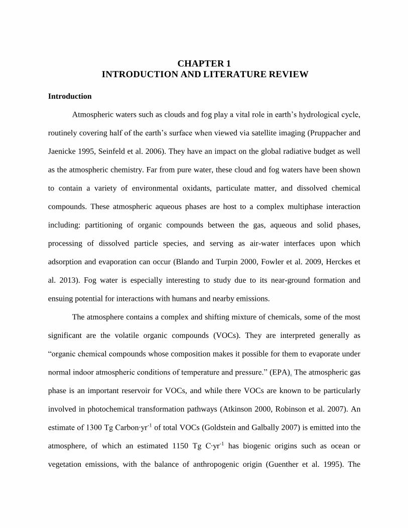
Introduction

Atmospheric waters such as clouds and fog play a vital role in earth’s hydrological cycle,

routinely covering half of the earth’s surface when viewed via satellite imaging (Pruppacher and

Jaenicke 1995, Seinfeld et al. 2006). They have an impact on the global radiative budget as well

as the atmospheric chemistry. Far from pure water, these cloud and fog waters have been shown

to contain a variety of environmental oxidants, particulate matter, and dissolved chemical

compounds. These atmospheric aqueous phases are host to a complex multiphase interaction

including: partitioning of organic compounds between the gas, aqueous and solid phases,

processing of dissolved particle species, and serving as air-water interfaces upon which

adsorption and evaporation can occur (Blando and Turpin 2000, Fowler et al. 2009, Herckes et

al. 2013). Fog water is especially interesting to study due to its near-ground formation and

ensuing potential for interactions with humans and nearby emissions.

The atmosphere contains a complex and shifting mixture of chemicals, some of the most

significant are the volatile organic compounds (VOCs). They are interpreted generally as

“organic chemical compounds whose composition makes it possible for them to evaporate under

normal indoor atmospheric conditions of temperature and pressure.” (EPA). The atmospheric gas

phase is an important reservoir for VOCs, and while there VOCs are known to be particularly

involved in photochemical transformation pathways (Atkinson 2000, Robinson et al. 2007). An

estimate of 1300 Tg Carbon∙yr-1 of total VOCs (Goldstein and Galbally 2007) is emitted into the

atmosphere, of which an estimated 1150 Tg C∙yr-1 has biogenic origins such as ocean or

vegetation emissions, with the balance of anthropogenic origin (Guenther et al. 1995). The

2

biogenic volatile organic compounds (BVOCs) are comprised of: monoterpenes (44%), isoprene

(11%), other reactive VOC (ORVOC) (22.5%), and other VOC (OVOC) (22.5%). While

monoterpene and isoprene emissions have good estimates, large uncertainties exist for estimates

of the latter two categories, and only a portion of VOC emissions in these categories are

speciated. By 1987, atmospheric measurements had identified tens of thousands of VOCs in the

ORVOC and OVOC categories (Graedel 1978, Graedel 1986) – still only a fraction of those

thought to exist - yet only a small portion of them have been studied.

Of the ORVOCs, one of the most significant groups are green leaf volatiles (GLVs),

emitted by many plants including: grass, oak, orange, clover, onion, and lettuce (Arey et al.

1991, Kirstine et al. 1998). These oxygenated, low molecular weight hydrocarbons are formed in

plants in the bio-catalyzed conversion of the omega-6 fatty acid linoleic acid. (Matsui 2006,

Hamilton et al. 2009) and play a role in signaling between plants (Matsui 2006). While healthy

plants emit only trace amounts, they are emitted in greatly enhanced quantities if the plant

undergoes stress such as mechanical agitation, temperature changes, and animal or insect grazing

(Kirstine et al. 1998, Farag and Pare 2002). GLVs have also been shown to have antimicrobial

properties and can even limit herbivores by recruiting their carnivorous enemies (Shiojiri et al.

2006). The most prevalent appear to be C6-oxygenates (Hamilton et al. 2009). Atmospheric

mixing ratios for GLVs have been estimated from 100-900 ppt (Williams et al. 2001, Jardine et

al. 2010, Kim et al. 2010), a potentially significant portion of the estimated 1-3 ppb (Kesselmeier

and Staudt 1999) mixing ratio allotted for ORVOCs.

While the umbrella term GLV covers many compounds and their derivatives, the focus

was on five GLVs crucial to the stress response (Arey et al. 1991, Harley et al. 1998, Heiden et

al. 1999, Preston et al. 2001): methyl jasmonate (MeJa), methyl salicylate (MeSa), 2-methyl-3-

3

buten-2-ol (MBO), cis-3-hexen-1-ol (HxO), and cis-3-hexenylacetate (HxAC). While to our

knowledge MeJa has not been detected in forests it is emitted in the vapor phase (Preston et al.

2001), and MBO, HxAC, HxO, and MeSa all have been detected over active vegetation.

(Williams et al. 2001, Jardine et al. 2010, Kim et al. 2010). Their structures are shown in Figure

1, and their basic properties are shown in Table 1. They have been shown to participate in gas

phase reactions with ozone and hydroxyl radicals (Hamilton et al. 2009, Harvey et al. 2014).

This is particularly interesting because it hints at their potential to participate in aqueous phase

photochemical reactions and form heavier molecular weight products (Richards-Henderson et al.

2014).

Figure 1. Molecular Structures of (a) methyl jasmonate (MeJa), (b) cis-3-hexenylacetate

(HxAC), (c) cis-3-hexen-1-ol (HxO), (d) methyl buten-2-ol (MBO), and (e) methyl salicylate

(MeSa)

Table 1. Basic Properties of GLVs.

GLV CAS

Number

Molecular

Formula

Molecular Weight

[g∙mol-1]

Boiling Point [°C]

Density at 25°C

[g∙mL-1]

MeJa 39924-52-2 C13H20O3 224.3 110 1.03

MeSa 119-36-8 C8H8O3 152.15 222 1.174

MBO 115-18-4 C5H10O 86.13 98-99 0.824

HxO 928-96-1 C6H12O 100.16 156-157 0.848

HxAC 3681-71-8 C8H14O2 142.19 75-76 0.897

4

Fog Water

Radiation fogs (of the type found in Baton Rouge) are formed when the ground surface

cooled by its emission of thermal radiation contacts and cools air supersaturated with water

vapor, instigating vapor condensation around nearby particulates. These droplets have

approximate diameters of 1-10 µm (Valsaraj 2012). The density of the fog is characterized by its

liquid water content, defined as the mass of water in the liquid phase per volume of dry air,

which can range from 0.02 to 1 [g∙m-3] (Seinfeld and Pandis 1998), and in Baton Rouge was

measured to be 0.008 – 0.33 [g∙m-3] (Raja et al. 2009). Samples of fog water have been collected

worldwide and have been found to contain significant amounts of organic carbon (1 – 200 mg

C∙L-1 aqueous volume) (Herckes et al. 2013), an estimated 75% of which is dissolved. This

dissolved portion includes a substantial amount of speciated carboxylic acids and carbonyls, but

often the majority of DOC are unidentified organic molecules (Herckes et al. 2013). Fog droplets

also contains solid particles which enter through collision or by becoming the associated

nucleation site upon which the fog droplet grows by condensation (Herckes et al. 2013). In

addition to organic carbon, fog also contains environmentally generated oxidants like hydroxyl

radicals which enter the droplet via the gas phase or are produced inside the droplet from the

hydrogen peroxide and other reactive species.

While much of the work regarding kinetics of aqueous phase oxidation reactions has been

done in the bulk phase, the reactions of compounds which may reside and react at the air-water

interface are less explored. Surface active compounds adsorbed to the air-water interface can be

present at the surface in large enough amounts to be considered a “surface phase”, significant

numbers of absolute mols relative to the bulk for small aqueous droplets (Valsaraj 2009). Recent

molecular dynamics simulations have shown that some GLV orientations occupy a free energy

5

minimum at the air-water interface (Liyana-Arachchi et al. 2013, Liyana-Arachchi et al. 2013,

Liyana-Arachchi et al. 2014). Additionally, surface reactions have been shown to have enhanced

reaction rates compared to the bulk (Chen et al. 2006, Richards-Henderson et al. 2014). This can

be understood intuitively: a molecule in complete dissolution in the bulk phase has a “cage” of

water molecules around it, in an orientation minimizing the Gibbs Free Energy. In order to react

with it, an oxidant must diffuse to and through this barrier; a heterogeneous reaction at the air-

water interface between adsorbed or only partially dissolved reactants does not face these

barriers. Surface active compounds can be detected because they decrease the surface tension of

a compound by interrupting the hydrogen bonding at the surface. Measurements show the

surface tension of fog water is less than that of pure water (Facchini et al. 2000) indicating the

presence of surface active compounds.

Secondary Organic Aerosols

VOCs processing in fog is significant here because it has been shown to lead to the

formation of secondary organic aerosol (SOA) (Volkamer et al. 2006, Hallquist et al. 2009,

Ervens et al. 2011). SOA is introduced into the atmosphere via chemical reactivity, they differ

from primary organic aerosols, which enter the atmosphere directly as dust, ocean salt from sea

sprays, volcanic emissions, or industrial anthropogenic emissions (Chin et al. 2009). The

formation of SOA inside atmospheric aqueous droplets has been linked to the oxidation of

dissolved volatile organic matter (Hallquist et al. 2009, Mentel et al. 2013). The oxidation of

DOC in aqueous atmospheric aerosols results not only in the formation of low weight molecular

compounds but also in the formation of higher molecular weight products by oligomerisation

(Hall and Johnston 2010). These lower volatility products may then partition into the particle

phase, or could aggregate and reach a high enough molecular mass to be considered SOA. SOAs

6

are significant because they affect respiratory health in animals (Mauderly and Chow 2008),

reduce visibility, and have a significant yet poorly understood radiative forcing effect (Change

2013). Their complex radiative behavior results from their varied composition and origin – black

carbon aerosols absorb radiation, but other organic aerosols reflect it (Kanakidou et al. 2005).

Additionally they serve as cloud condensation nuclei (CCN) thus participating in the atmospheric

water cycle and indirectly affecting the radiation budget. Their role as CCN gives rise to the so-

called fog-smog-fog cycle whereby fog droplets are formed, process VOCs and produce SOA,

settle gravitationally then evaporate – leaving behind more aerosols at ground level to serve as

new CCN (Munger et al. 1983). While GLVs formation of SOA has been investigated in the gas

phase (Hamilton et al. 2009), their role in aqueous phase SOA production has only recently been

explored (Richards-Henderson et al. 2014).

Partitioning and Equilibrium Properties

Equilibrium physico-chemical properties allow the determination of the direction and

magnitude of the thermodynamic coercion on a molecule in the environment. Upon the

formation of a fog droplet, a complex interplay of physical processes begins in and around the

newly formed aqueous phase. This is shown in Figure 2 below. The soluble portion of the

particulate nucleus begins to dissolve, gases including both VOCs and oxidants from the

surrounding air meet the air-water interface and are adsorbed or absorbed, reactions between

various dissolved compounds begin, and the droplet itself grows, contracts, and collides with

other droplets. The extent of the partitioning of a VOC into each of the three compartments: air,

bulk aqueous, and air-water interface at equilibrium is vital to understanding an analyte’s

environmental fate and thus its potential to produce SOA. The relationships between each of the

three compartments are represented by partition coefficients as shown in Figure 3 below.

7

Figure 2. Physical processes occurring in a dispersed aqueous phase.

Figure 3. The relationship between the three phase concentrations and their partition coefficients.

8

The ratio of bulk aqueous concentration CW to gas phase concentration CA for an analyte

in an air-water system at equilibrium is governed by its Henry’s Constant KH [M/atm], an

extremely important parameter in determining the eventual fate of a compound in the

environment. Likewise a compound’s concentration ratio between the surface to bulk aqueous

compartments is given by KSW and its concentration ratio between surface to air compartments is

KSA. In this way, if the concentration in one phase of an air-water system is known, the others

can be found. A compound’s octanol-water partition coefficient log(KOW), defined as the

concentration ratio of an analyte in a system of mutually saturated octanol and water, is another

important partition measure, indicating an analyte’s hydrophobicity (Valsaraj 2009). It can be

correlated to find soil/water and gas-to-particle partitioning in the atmosphere. Finally a

compound’s saturated aqueous solubility, S [mM], is an important equilibrium value used to

express hydrophilicity and determine the extent to which it is possible for an analyte to partition

into the aqueous phase – relevant here because an analyte partitioning into fog may be limited by

its solubility S.

Research Objective

This research aims to experimentally determine and evaluate estimations for the physico-

chemical properties of the five chosen GLVs, and in doing so elucidate their partitioning

behavior and environmental fate. For each chosen GLV, the Henry’s Constant KH at three

different temperatures and ionic strengths, their enthalpy and entropy of phase change, and their

aqueous solubility were measured. While measured KH values can be found in the literature for

most GLVs, they have been measured only at 25°C in pure water (above the temperature of fog

formation). In order to be relevant for environmental conditions of fog formation, KH must be

measured at different temperatures and ionic strengths. Additionally these parameters will be

9

predicted using prominent estimation methods and software for which GLVs present an excellent

test case because they are all multifunctional oxygenated alkenes which may have complex polar

character. This work includes: measurements of KH at various temperatures and ionic strengths,

aqueous solubility determination, and estimations of log(KOW), S, and KH for these five GLVs:

methyl jasmonate (MeJa), methyl salicylate (MeSa), 2-methyl-3-buten-2-ol (MBO), cis-3-hexen-

1-ol (HxO), and cis-3-hexenylacetate (HxAC).

10

CHAPTER 2

PHYSICO-CHEMICAL PROPERTY ESTIMATION METHODS

Introduction

As mentioned in Chapter 1, values of physico-chemical properties are vital to

understanding the fate and transport of chemicals in the environment. For many compounds of

interest, experimentally measured values of these properties are not available, so there exist a

variety of methods to estimate them. They can be divided loosely into two categories:

quantitative structure property relationships (QSPR), and quantitative physical property

relationships (QPPR). Estimations of both types are used not only for smaller functional organic

molecules of environmental interest, but also complex, multifunctional molecules and

pharmaceutical drugs.

QSPRs are based on the tenet that a compound’s thermodynamic properties are the

consequence of its atomic makeup and molecular structure. Each molecular attribute in the

molecule is assigned a contribution value, and the contributions from all of attributes in a

molecule are summed to estimate the desired property. Two main types exist; bond contribution

schemes count each individual bond and are applicable to a wide range of compounds, while

group contribution methods count only functional groups. Group contribution approaches are

generally regarded as more accurate (Staudinger and Roberts 1996), but also more limited

because they fail to give a result if a compound contains a functional group which is not in their

dataset. Group contributions are also often trained on datasets containing monofunctional

compounds so as to isolate and ascertain the effect of a single functional group, and thus can

misestimate by neglecting effects of adjacency or a molecule’s overall complex polar character.

Both can be made more accurate by limiting the training set to compounds of a certain class, at

the expense of general usefulness - many environmentally relevant compounds have multiple

11

functionalities (for instance the GLVs in this paper). In general both group and bond contribution

methods will be more inaccurate the more complex the molecule is.

QPPRs correlate separate known or estimated physico-chemical properties such as

solubility, or molecular descriptors such as surface area to find the desired property. These can

be simple correlations with a known measured property, or large poly-parameter models using a

variety of estimated and calculated properties. They can be derived from fundamental

thermodynamics or simply reflect an observed correlation. QPPRs also frequently combine

molecular structural and functional group or structural properties as in QSPRs with physic-

chemical descriptors as found in to estimate a parameter, and thus the division between QSPRs

and QPPRs is not definite.

Henry’s Constant

Henry’s Constant is most easily estimated by taking a vapor pressure to solubility ratio,

however neither of these values are available for GLVs, and estimating both to in turn estimate

KH would introduce a large error. Many bond contribution methods exist (Cramer 1980, Cabani

et al. 1981, Modarresi et al. 2007), here two prominent and easy to use methods were applied to

predict KH: that of Hine & Mookerjee (1975) (Hine and Mookerjee 1975) and the HENRYWIN

program (Meylan and Howard 1991) from the Environmental Protection Agency’s Estimation

Property Interface Suite (referred to here as HENRYWIN-BOND). HENRYWIN-BOND is

based on an updated version of Hine & Mookerjee’s original protocol, with an expanded training

set and corrections for problematic functional groups. HENRYWIN’s group contribution method

(HENRYWIN-GROUP) was also used, based exactly on Hine & Mookerjee’s original protocol.

Two methods combining molecular connectivity indices, group contributions, and polarizability

were also used: those of Nirmalakhandan et al. (Nirmalakhandan et al. 1997) and Suzuki et al.

12

(Suzuki et al. 1992). These methods use information about molecular configuration in their

calculations, and are thus able to recognize differences between isomers. While many QPPRs

exist for KH determination (Russell et al. 1992, Abraham et al. 1994, Schüürmann 1995, Dearden

and Schüürmann 2003), but they often require unavailable or demanding calculations of

molecular parameters to use. Thus, the only QPPR used for KH determination was SPARC

Performs Analytical Reasoning in Chemistry (SPARC) online calculator based on a blend of

Linear Free Energy Relationships and Perturbed Molecular Orbital theory (Hilal et al. 2003).

Solubility

Many estimations were performed to obtain the aqueous solubility of GLVs including:

EPI Suite’s WATERNT bond contribution method (Meylan and Howard 1995), the group

contribution method of Marrero & Gani (Marrero and Gani 2002), and SPARC. In addition, the

logarithm of solubility log(S) is also commonly estimated by using correlations with either

experimentally determined or estimated log(KOW) values. The relation arises by manipulating the

fugacity equations of an analyte in solution and octanol, eventually giving Equation 1. (Chiou et

al. 1982)

log(𝐾𝑂𝑊) = − log(𝑆) − log(��𝑂∗) − log(𝛾��) + log (

𝛾��

𝛾𝑊) (1)

��𝑂∗ is the molar volume of octanol saturated with water, 𝛾�� is the activity coefficient of the solute

in octanol saturated with water, 𝛾�� is the solute activity coefficient in water saturated with

octanol, and 𝛾𝑊 is the solute activity coefficient in pure water. If one assumes that the solute

forms an ideal solution in octanol, and that the analyte’s solubility is the same in pure water as

water saturated with octanol, then the latter two terms in Equation 1 drop out and log(KOW) can

be directly correlated with log(S) with an ideal-case slope of -1. The full derivation is given in

Appendix A. Numerous coefficients for this QPPR have been published; coefficients from the

13

following sources were used in this work: EPI Suite’s WSKOW program (Meylan and Howard

1996), Chiou et al. (Chiou et al. 1977), Banerjee et al. (Banerjee et al. 1980), and Isnard and

Lambert (Isnard and Lambert 1989). Finally, Jain et al. (Jain et al. 2001) presents the General

Solubility Equation which begins by defining KOW as the solubility of the analyte in octanol, CO,

divided by the analyte solubility in water, S. By assuming all organic analytes are fully miscible

in octanol, a simple correlation between log(S) and log(KOW) is found.

Octanol-water Partition Coefficient

The methods used to estimate log(KOW) were the group contribution of Marrero et al.

(Marrero and Gani 2002), the KOWWIN method from EPI Suite (Meylan and Howard 1995),

SPARC, and the correlations used above to estimate log(S) from log(KOW).

14

CHAPTER 3

MATERIALS AND METHODS

Chemicals

Pure samples of each GLV, viz., Methyl Jasmonate (95%), Methyl Salicylate (Reagent

plus®, ≥ 99%), 2-methyl-3-buten-2-ol (98%), cis-3-hexen-1-ol (natural, ≥ 98 %) and cis-3-

hexenylacetate (≥98%) were obtained from Sigma-Aldrich© and used as received without further

purification. Ammonium Nitrate (ACS Reagent, ≥98%), Sodium Hydroxide (Sigma-Aldrich,

99.998%), Sulfuric Acid (BDH, ACS Grade 95-98%) and Ammonium Chloride (ACROS

Organics, 99.5%) were used in ionic strength experiments. LC-MS grade water (Honeywell, B&J

Brand®) was used to make solutions. Acetonitrile used was from EMD Millipore© (HPLC grade,

≥99.8%).

In order to test the ionic strength effects, ionic solutions were prepared based on the ionic

content found in fog waters sampled at Baton Rouge (LA, USA) (Raja et al. 2005): NO3- (3

mM), SO42- (2 mM), Na+ (3.3 mM), Cl- (3 mM), and NH4

+ (6 mM). Additionally, ionic solutions

concentrated by a factor 100 were also used based on the same composition. The ionic solutions

have a pH value of 6.

Chemical analysis

All aqueous sample analyses were conducted using HPLC analysis. An Agilent 1100

HPLC-UV/DAD system was used consisting of the following components: a degasser

(G1322A), a quaternary pump (G1311A), an autosampler (G1313A), a column compartment

(G1316A) and a diode array detector (G1315A). 4 µL of each sample was injected into a 2.1 mm

x 150 mm Pinnacle II PAH column (Restek Corp., Bellefonte, PA, USA) with 4µm particle size,

held at 40 C. A water:acetonitrile gradient method with a flow-rate of 0.2 mL·min-1 was used,

15

starting with 60% acetonitrile for one minute, ramping linearly to 100% acetonitrile over 6

minutes, followed by a three minute isocratic hold at 100% acetonitrile, and a final ramping

down to 60% acetonitrile over 3 minutes, followed by an 8 minute post time at 60% acetonitrile.

The UV absorbance of the GLVs was monitored with an average signal at 195 nm for MeJa,

MBO, HxO, and HxAC and at 210 nm for MeSa, taking a data point every 2 seconds using the

diode array detector with a slit width of 4 nm. The concentration was determined from the

measured peak area via a calibration curve obtained from the analysis of standard solutions of

known concentrations from 0.2-140 mg·L-1.

Determination of Henry’s Law Constants

Henry’s law constants were measured using a modified liquid stripping technique

developed in the past for semi-volatile organic compounds (Mackay et al. 1979, Bamford et al.

1999). Figure 4 is a schematic of the equipment used.

Figure 4. Gas Stripping Apparatus for Measurement of Henry’s Constant for GLVs.

Ultra high purity compressed air (Alphagaz 1, Air Liquide©) was passed through a flow-meter

(Cole Parmer PMR-1) at 30-45 mL/min before entering a 1 L gas-washing bottle containing LC-

MS grade water to saturate the air with water vapor. The air was then bubbled through a coarse

16

frit at the bottom of a glass bubble column (100 cm length and 5 cm inside diameter) filled with

an aqueous solution of GLV to a liquid height of 75 cm. Solutions of GLV were prepared in 3

media: deionized water, ionic solution based on concentration given above, and ionic solution

concentrated by a factor 100. The solutions were used in separate Henry’s Constant experiments,

to determine the effect of ionic strength on the air-water partitioning of each GLVs.

The air bubbles reached equilibrium as they progressed vertically through the column,

passed through a glass impactor to remove any solid and liquid aerosols caused by bursting

bubbles, and then through an XAD-2 polymeric resin trap (ORBO 43 Supelpak-20, Sigma-

Aldrich) to collect airborne GLVs. Each trap has a front and back section; measuring the GLV

concentration in these sections separately showed that the maximum GLV found in the back

section was less than 5%. For this experiment, both front and back were used. The column was

wrapped in a water jacket and insulated to maintain a stable aqueous temperature. The GLVs

were desorbed from the XAD-2 trap by soaking in 10 mL of acetonitrile and shaking for two

hours. The resulting solution was filtered (PTFE filter, porosity of 0.45 µm, Whatman XD/G)

and analyzed by HPLC. Photographs of the top of the column are shown in Figure 5. Sampling

intervals ranged from 15 minutes to 24 hours, and at each time point aqueous samples were

taken, the temperature was checked, and the sorbent trap was replaced with a new one. The first

time point was not included in data analysis because adsorptive effects of the GLV on the top of

the apparatus were apparent, and the determined KH was higher than all of the others. The ratio

of the average aqueous concentration (CW) to the measured air concentration (CA) was used to

obtain the Henry’s Law constant, KH [M·atm-1].

17

Figure 5. (a) The top of the column, not including XAD-2 trap (b) close-up view of aerosol

impactor and XAD-2 resin gas trap.

Determination of Saturation Aqueous Solubility

Aqueous solubility S [mM] was measured using a traditional batch equilibration shake

flask technique (Banerjee et al. 1980). Ten 40 mL amber borosilicate vials with PTFE lined caps

(VWR 93001-538) were each filled with 35 mL LC-MS grade water. GLV was added to each

vial in increasing amounts, with the highest mass added corresponding to double the solubility

estimated by the WATERNT program from EPI Suite (EPA 2012). The sealed vials were

allowed to equilibrate over several days while gently shaken in a water bath at 25°C. After the

equilibration period, the shaker was turned off, and the samples kept in the bath for 24 hours, to

allow un-dissolved solute to settle to the bottom or rise to the top. Aliquots of 2 mL were taken

from the middle of the liquid volume and centrifuged at 12,000 rpm for 15 minutes. Aqueous

samples were then taken from the aliquots and diluted for analysis with HPLC. As the solubility

18

limit was approached and passed, the aqueous concentration plateaued. The solubility limit was

determined as the average of these plateau increased GLV concentrations until the plateau was

apparent.

19

CHAPTER 4

RESULTS AND DISCUSSION

Henry’s Law Constants at 25°C

Henry’s law is the relationship between the equilibrium concentrations of a compound in

the aqueous and air phases. The air stripping technique used requires that the method be first

validated using a compound of known Henry’s constant. In this case we chose an aromatic

compound, viz., benzene. Using the instrumentation described in this work, the measured KH of

benzene is 0.19 ± 0.03 M·atm-1 which compares well with literature values of 0.19 – 0.21 M·atm-

1 (Mackay et al. 1979, Ashworth et al. 1988, Dewulf et al. 1995, Karl et al. 2003). Measurements

of the gas phase and aqueous phase concentrations were made at regular intervals and the ratio of

gas to aqueous phase concentration are plotted as shown in Figure 6 for a typical run for MeSa.

Time [minutes]

0 20 40 60 80 100 120 140 160 180 200

MeS

a K

H [M

·atm

-1]

0

10

20

30

40

50

60

70

Figure 6. MeSa KH vs Time at 25°C showing asymptotic values.

20

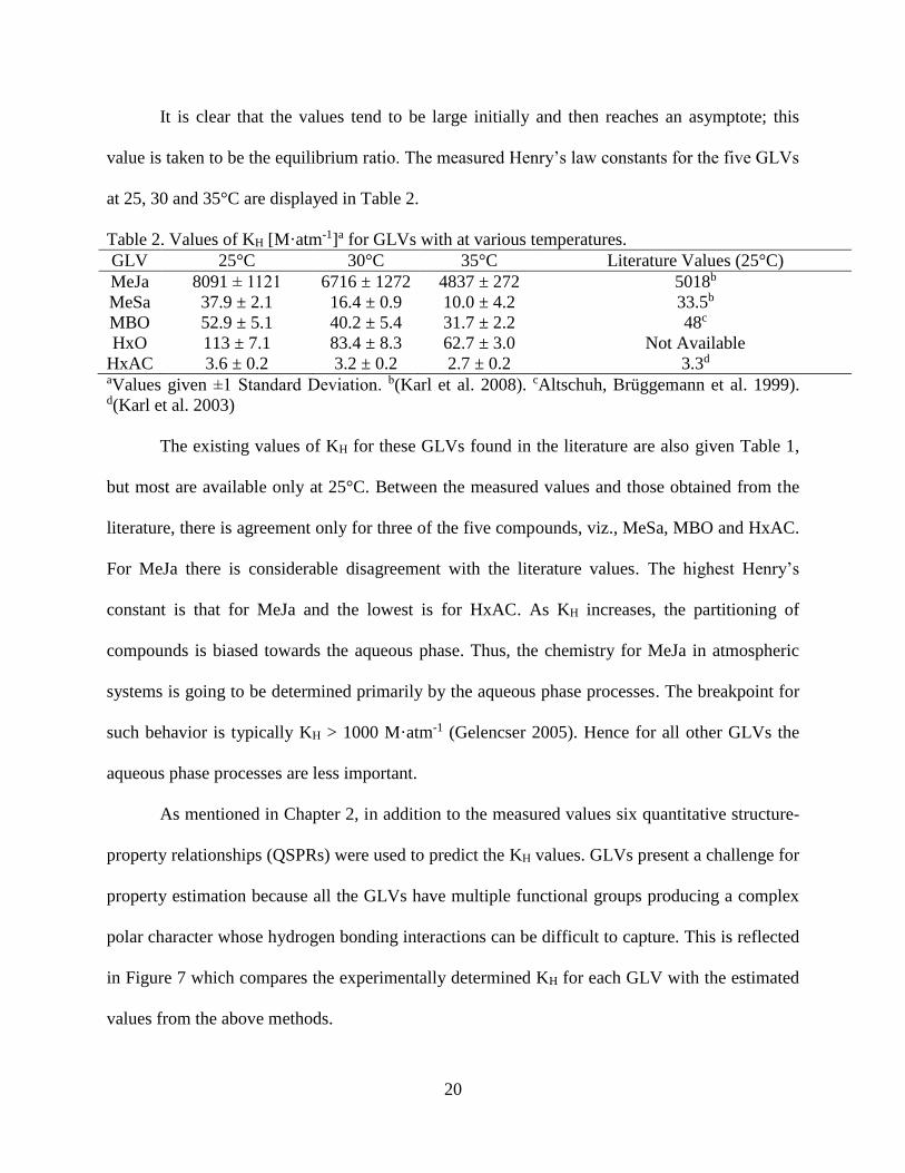
It is clear that the values tend to be large initially and then reaches an asymptote; this

value is taken to be the equilibrium ratio. The measured Henry’s law constants for the five GLVs

at 25, 30 and 35°C are displayed in Table 2.

Table 2. Values of KH [M·atm-1]a for GLVs with at various temperatures.

GLV 25°C 30°C 35°C Literature Values (25°C)

MeJa 8091 ± 1121 6716 ± 1272 4837 ± 272 5018b

MeSa 37.9 ± 2.1 16.4 ± 0.9 10.0 ± 4.2 33.5b

MBO 52.9 ± 5.1 40.2 ± 5.4 31.7 ± 2.2 48c

HxO 113 ± 7.1 83.4 ± 8.3 62.7 ± 3.0 Not Available

HxAC 3.6 ± 0.2 3.2 ± 0.2 2.7 ± 0.2 3.3d

aValues given ±1 Standard Deviation. b(Karl et al. 2008). cAltschuh, Brüggemann et al. 1999). d(Karl et al. 2003)

The existing values of KH for these GLVs found in the literature are also given Table 1,

but most are available only at 25°C. Between the measured values and those obtained from the

literature, there is agreement only for three of the five compounds, viz., MeSa, MBO and HxAC.

For MeJa there is considerable disagreement with the literature values. The highest Henry’s

constant is that for MeJa and the lowest is for HxAC. As KH increases, the partitioning of

compounds is biased towards the aqueous phase. Thus, the chemistry for MeJa in atmospheric

systems is going to be determined primarily by the aqueous phase processes. The breakpoint for

such behavior is typically KH > 1000 M·atm-1 (Gelencser 2005). Hence for all other GLVs the

aqueous phase processes are less important.

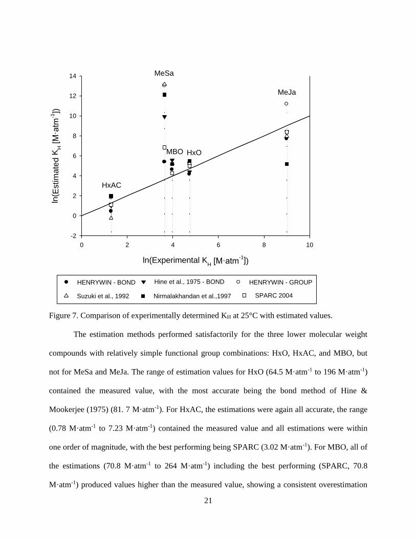
As mentioned in Chapter 2, in addition to the measured values six quantitative structure-

property relationships (QSPRs) were used to predict the KH values. GLVs present a challenge for

property estimation because all the GLVs have multiple functional groups producing a complex

polar character whose hydrogen bonding interactions can be difficult to capture. This is reflected

in Figure 7 which compares the experimentally determined KH for each GLV with the estimated

values from the above methods.

21

ln(Experimental KH [M·atm

-1])

0 2 4 6 8 10

ln( E

stim

ate

d K

H [

M·a

tm-1

])

-2

0

2

4

6

8

10

12

14

HxAC

MeSa

MBO HxO

MeJa

HENRYWIN - BOND HENRYWIN - GROUP Hine et al., 1975 - BOND

Suzuki et al., 1992 Nirmalakhandan et al.,1997 SPARC 2004

Figure 7. Comparison of experimentally determined KH at 25°C with estimated values.

The estimation methods performed satisfactorily for the three lower molecular weight

compounds with relatively simple functional group combinations: HxO, HxAC, and MBO, but

not for MeSa and MeJa. The range of estimation values for HxO (64.5 M·atm-1 to 196 M·atm-1)

contained the measured value, with the most accurate being the bond method of Hine &

Mookerjee (1975) (81. 7 M·atm-1). For HxAC, the estimations were again all accurate, the range

(0.78 M·atm-1 to 7.23 M·atm-1) contained the measured value and all estimations were within

one order of magnitude, with the best performing being SPARC (3.02 M·atm-1). For MBO, all of

the estimations (70.8 M·atm-1 to 264 M·atm-1) including the best performing (SPARC, 70.8

M·atm-1) produced values higher than the measured value, showing a consistent overestimation

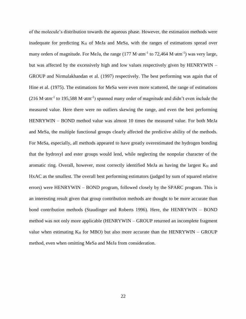
22

of the molecule’s distribution towards the aqueous phase. However, the estimation methods were

inadequate for predicting KH of MeJa and MeSa, with the ranges of estimations spread over

many orders of magnitude. For MeJa, the range (177 M·atm-1 to 72,464 M·atm-1) was very large,

but was affected by the excessively high and low values respectively given by HENRYWIN –

GROUP and Nirmalakhandan et al. (1997) respectively. The best performing was again that of

Hine et al. (1975). The estimations for MeSa were even more scattered, the range of estimations

(216 M·atm-1 to 195,588 M·atm-1) spanned many order of magnitude and didn’t even include the

measured value. Here there were no outliers skewing the range, and even the best performing

HENRYWIN – BOND method value was almost 10 times the measured value. For both MeJa

and MeSa, the multiple functional groups clearly affected the predictive ability of the methods.

For MeSa, especially, all methods appeared to have greatly overestimated the hydrogen bonding

that the hydroxyl and ester groups would lend, while neglecting the nonpolar character of the

aromatic ring. Overall, however, most correctly identified MeJa as having the largest KH and

HxAC as the smallest. The overall best performing estimators (judged by sum of squared relative

errors) were HENRYWIN – BOND program, followed closely by the SPARC program. This is

an interesting result given that group contribution methods are thought to be more accurate than

bond contribution methods (Staudinger and Roberts 1996). Here, the HENRYWIN – BOND

method was not only more applicable (HENRYWIN – GROUP returned an incomplete fragment

value when estimating KH for MBO) but also more accurate than the HENRYWIN – GROUP

method, even when omitting MeSa and MeJa from consideration.

23

Henry’s Law Constants at varying temperature

The variation of the Henry’s constants with temperature is an important parameter in the

assessment of the atmospheric aqueous chemistry. The variation can be expressed using

Equation 2 (Valsaraj 2009).

ln 𝐾𝐻 = 𝐴 −𝐵

𝑇 (2)

A and B are constants and T is temperature [K]. From the constants A and B, the enthalpy of

phase change from liquid to gas ∆H [kJ·mol-1] and the entropy of phase change ∆S [kJ·mol-1·K-

1] for each compound can be found (Bamford et al. 1999). The results are shown in Table 3.

Table 3. Measured enthalpy and entropy of phase change each GLV from T varied KH.

GLV A B ∆H (kJ·mol-1)a ∆S (J·mol-1·K-1)b r2

MeJa -0.1015 4719.5 36.7 ± 13.2 21.6 ± 21.8 0.969

MeSa 30.50 12221 99.1 ± 28.3 276 ± 47 0.980

MBO 4.913 4706.2 36.6 ± 2.5 63.2 ± 4.2 0.999

HxO 6.518 5412.1 42.5 ± 0.8 76.6 ± 1.3 0.999

HxAC 2.278 3126.3 23.5 ± 10.3 41.3 ± 17.3 0.954 aValues given ±2 Standard Errors of the slope. bValues given ±1 Standard Errors of the intercept

The ∆H values ranged from (23.5 ± 10.3) kJ·mol-1 to (99.1 ± 28.3) kJ·mol-1 for HxAC

and MeSa respectively. These are consistent with the ∆H of non-aromatic, oxygenated alkenes

(Chickos and Acree 2003). For MBO, HxO, and HxAC they are similar to enthalpy of

vaporization for unsaturated counterparts: 50.3 kJ·mol-1 for 2-methyl-2-butanol, 61.1 kJ·mol-1

for 1-hexanol, and 52.1 kJ·mol-1 for hexyl acetate (Chickos and Acree 2003). Double bonds have

been shown to decrease the enthalpy of vaporization but generally only by 1-2 kJ·mol-1 for

alkanes (Baev 2012). The rest of the discrepancy may be attributed to the fact that the cited

values of enthalpy of vaporization are calculated as the energy required to vaporize the pure

compound from its pure liquid, however the enthalpy required to vaporize the GLV from an

aqueous solution may be higher due to hydrogen bonding. The ∆H of MeSa compares favorably

with that of other oxygenated aromatics such as benzoic acid (89.5 ± 0.16) kJ·mol-1 (Morawetz

24

1972). The ∆S values ranged from (22 ± 21) J·mol-1·K-1 (MeJa) to (276 ± 47) J·mol-1·K-1

(MeSa). MeJa, HxO, MeSa, and HxAC have values within the expected range for organic

compounds, while MeSa’s high value compares well with that of benzoic acid (261 J·mol-1·K-1)

(Torres-Gómez et al. 1988).

Henry’s Law Constants at varying ionic concentrations

In the literature it has been reported that KH for glyoxal increases by as much as 50 times

in the presence of sodium sulfate (Ip et al. 2009). Hence, the extent to which partitioning

behavior of GLVs would be affected by environmentally relevant fog water composition was

determined by performing an experiment at ionic strength comparable to actual fog water. One

solution had an ionic composition similar to the fog water (0.01 M) and the other one had a

composition 100 times (1 M) comparable to that of an industrial wastewater. The KH obtained in

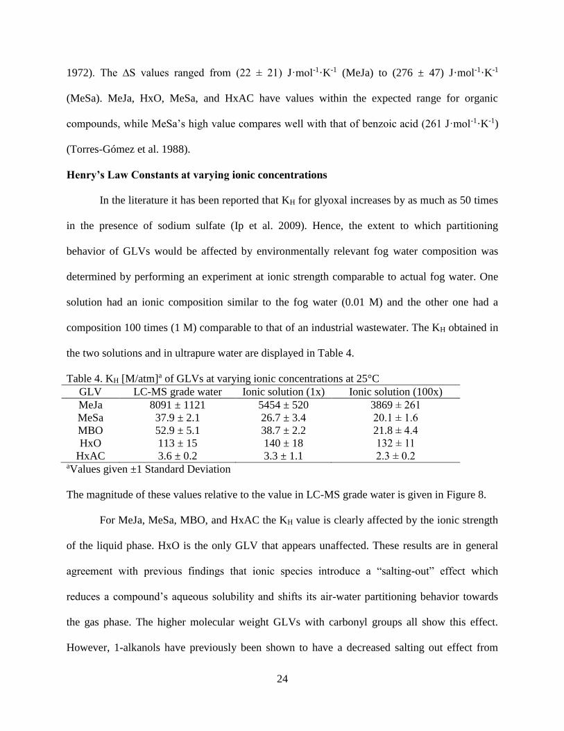
the two solutions and in ultrapure water are displayed in Table 4.

Table 4. KH [M/atm]a of GLVs at varying ionic concentrations at 25°C

GLV LC-MS grade water Ionic solution (1x) Ionic solution (100x)

MeJa 8091 ± 1121 5454 ± 520 3869 ± 261

MeSa 37.9 ± 2.1 26.7 ± 3.4 20.1 ± 1.6

MBO 52.9 ± 5.1 38.7 ± 2.2 21.8 ± 4.4

HxO 113 ± 15 140 ± 18 132 ± 11

HxAC 3.6 ± 0.2 3.3 ± 1.1 2.3 ± 0.2 aValues given ±1 Standard Deviation

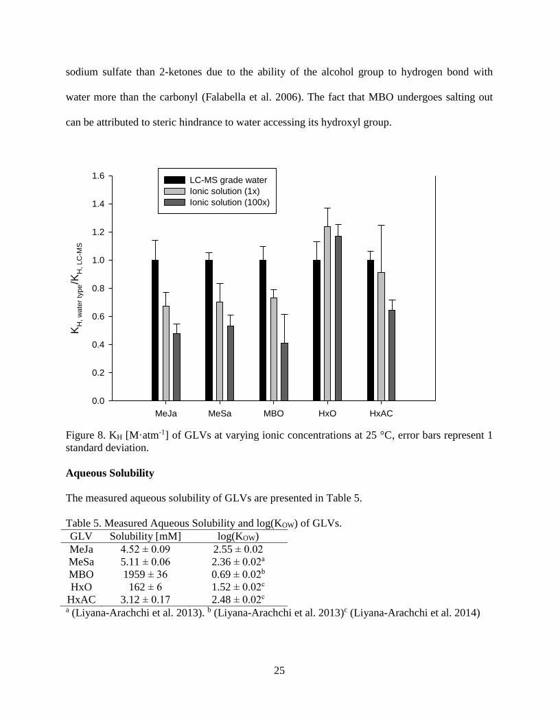
The magnitude of these values relative to the value in LC-MS grade water is given in Figure 8.

For MeJa, MeSa, MBO, and HxAC the KH value is clearly affected by the ionic strength

of the liquid phase. HxO is the only GLV that appears unaffected. These results are in general

agreement with previous findings that ionic species introduce a “salting-out” effect which

reduces a compound’s aqueous solubility and shifts its air-water partitioning behavior towards

the gas phase. The higher molecular weight GLVs with carbonyl groups all show this effect.

However, 1-alkanols have previously been shown to have a decreased salting out effect from

25

sodium sulfate than 2-ketones due to the ability of the alcohol group to hydrogen bond with

water more than the carbonyl (Falabella et al. 2006). The fact that MBO undergoes salting out

can be attributed to steric hindrance to water accessing its hydroxyl group.

MeJa MeSa MBO HxO HxAC

KH

, w

ate

r ty

pe/K

H,

LC

-MS

0.0

0.2

0.4

0.6

0.8

1.0

1.2

1.4

1.6LC-MS grade water

Ionic solution (1x)

Ionic solution (100x)

Figure 8. KH [M·atm-1] of GLVs at varying ionic concentrations at 25 °C, error bars represent 1

standard deviation.

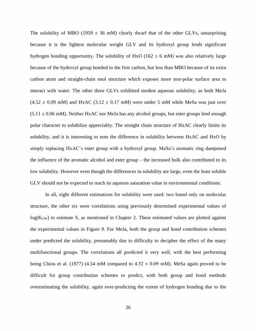
Aqueous Solubility

The measured aqueous solubility of GLVs are presented in Table 5.

Table 5. Measured Aqueous Solubility and log(KOW) of GLVs.

GLV Solubility [mM] log(KOW)

MeJa 4.52 ± 0.09 2.55 ± 0.02

MeSa 5.11 ± 0.06 2.36 ± 0.02a

MBO 1959 ± 36 0.69 ± 0.02b

HxO 162 ± 6 1.52 ± 0.02c

HxAC 3.12 ± 0.17 2.48 ± 0.02c a (Liyana-Arachchi et al. 2013). b (Liyana-Arachchi et al. 2013)c (Liyana-Arachchi et al. 2014)

26

The solubility of MBO (1959 ± 36 mM) clearly dwarf that of the other GLVs, unsurprising

because it is the lightest molecular weight GLV and its hydroxyl group lends significant

hydrogen bonding opportunity. The solubility of HxO (162 ± 6 mM) was also relatively large

because of the hydroxyl group bonded to the first carbon, but less than MBO because of its extra

carbon atom and straight-chain enol structure which exposes more non-polar surface area to

interact with water. The other three GLVs exhibited modest aqueous solubility, as both MeJa

(4.52 ± 0.09 mM) and HxAC (3.12 ± 0.17 mM) were under 5 mM while MeSa was just over

(5.11 ± 0.06 mM). Neither HxAC nor MeJa has any alcohol groups, but ester groups lend enough

polar character to solubilize appreciably. The straight chain structure of HxAC clearly limits its

solubility, and it is interesting to note the difference in solubility between HxAC and HxO by

simply replacing HxAC’s ester group with a hydroxyl group. MeSa’s aromatic ring dampened

the influence of the aromatic alcohol and ester group – the increased bulk also contributed to its

low solubility. However even though the differences in solubility are large, even the least soluble

GLV should not be expected to reach its aqueous saturation value in environmental conditions.

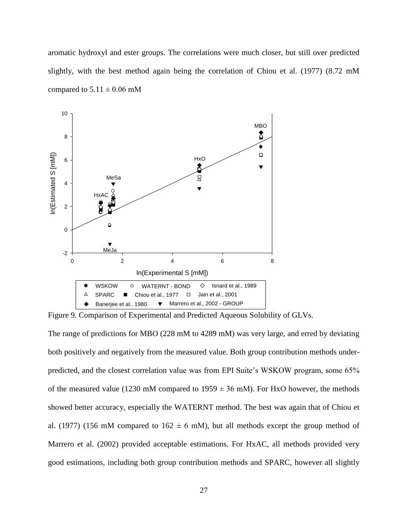
In all, eight different estimations for solubility were used: two based only on molecular

structure, the other six were correlations using previously determined experimental values of

log(KOW) to estimate S, as mentioned in Chapter 2. These estimated values are plotted against

the experimental values in Figure 9. For MeJa, both the group and bond contribution schemes

under predicted the solubility, presumably due to difficulty to decipher the effect of the many

multifunctional groups. The correlations all predicted it very well, with the best performing

being Chiou et al. (1977) (4.54 mM compared to 4.52 ± 0.09 mM). MeSa again proved to be

difficult for group contribution schemes to predict, with both group and bond methods

overestimating the solubility, again over-predicting the extent of hydrogen bonding due to the

27

aromatic hydroxyl and ester groups. The correlations were much closer, but still over predicted

slightly, with the best method again being the correlation of Chiou et al. (1977) (8.72 mM

compared to 5.11 ± 0.06 mM

ln(Experimental S [mM])

0 2 4 6 8

ln(E

stim

ate

d S

[m

M])

-2

0

2

4

6

8

10

HxAC

MeJa

MeSa

HxO

MBO

WSKOW WATERNT - BOND

Marrero et al., 2002 - GROUP

SPARC Chiou et al., 1977 Jain et al., 2001

Banerjee et al., 1980

Isnard et al., 1989

Figure 9. Comparison of Experimental and Predicted Aqueous Solubility of GLVs.

The range of predictions for MBO (228 mM to 4289 mM) was very large, and erred by deviating

both positively and negatively from the measured value. Both group contribution methods under-

predicted, and the closest correlation value was from EPI Suite’s WSKOW program, some 65%

of the measured value (1230 mM compared to 1959 ± 36 mM). For HxO however, the methods

showed better accuracy, especially the WATERNT method. The best was again that of Chiou et

al. (1977) (156 mM compared to 162 ± 6 mM), but all methods except the group method of

Marrero et al. (2002) provided acceptable estimations. For HxAC, all methods provided very

good estimations, including both group contribution methods and SPARC, however all slightly

28

overestimated the value. The closest came from WSKOW (4.39 mM compared to 3.12 ± 0.17

mM).

The two best performing estimations were those of Chiou et al. (1977) and EPI Suite’s

WSKOW program, both from measured log(KOW) values. Either the correlation of Chiou et al.

(1977) or WSKOW program had the best solubility estimation for every GLV. Overall, all

methods generally identified MBO as the most soluble, HxO as less soluble than MBO, and

MeSa, MeJa, and HxAC as far less. As in the prediction of Henry’s Constants, the group

contribution method appeared to struggle with both MeJa and MeSa, the two most complex

GLVs. This highlights a severe limitation with EPI Suite: its consistent inability to estimate the

properties multifunctional compounds like GLVs. EPI Suite is widely used in environmental

calculations but it’s clear that its estimations should be used with great caution. Since group

contribution methods predict properties “from scratch”, it is somewhat unfair to compare them to

the correlations based on accurate experimental values. Neither the Chiou et al. (1977) nor

WSKOW correlations used the ideal-case slope of -1 for the relation between log(KOW) and

log(S), yet were more accurate in this case than the other correlations which were closer to

ideality. Though in the idealized case the slope should be -1, others have found (Isnard and

Lambert 1989) that over a large training set this does not bear true. This discrepancy has been

attributed to non-ideal behavior resulting from the mutual saturation of water and octanol (Chiou

et al. 1982). This can be explained by examining Equation 1: while octanol is only slightly

soluble in water, water is highly soluble (2.3 M (Chiou et al. 1982)) in octanol which directly

affects molar volume ��O∗ and could affect the 𝛾�� term, depending on the analyte. Past papers

have found that grouping monofunctional compounds by class increases correlational accuracy

and pushes the slope toward unity (Tewari et al. 1982). However, for multifunctional compounds

29

like GLVs, using a general correlation trained on a varied dataset of compounds with a wide

variety of functional groups appears to be the best choice. This may be because of non-ideal

conditions as specified above affecting the process. When estimating the aqueous solubility of

multifunctional compounds such as GLVs, a correlation with an experimentally determined

log(KOW) is preferable to group contribution methods, as noted elsewhere (Meylan and Howard

1996).

1-Octanol/Water Partition Coefficient

In previous works from our laboratory, the log(KOW) values for MBO, HxO, HxAC, and

MeSa were measured (Liyana-Arachchi et al. 2013, Liyana-Arachchi et al. 2013, Liyana-

Arachchi et al. 2014). They are presented in Table 5 along with the measured value for MeJa.

The log(KOW) values reflected the solubility trends: the most soluble GLV (MBO) partitions

strongly to the aqueous phase, followed by the second most soluble (HxO), followed distantly by

MeJa, MeSa, and HxAC. These values are plotted in Figure 10 against the estimated values

mentioned in Chapter 2.

Here again, the Chiou et al. (1997) correlation is clearly the most accurate. This is

unsurprising, given that the KOWWIN and WATERNT estimations are both based on the same

bond/fragment contribution methodology (Meylan and Howard 1991), and the other correlations

fared worse than Chiou et al. (1977) in predicting log(S) from log(KOW). The correlation from

Chiou et al. (1977) was the most accurate for every GLV except HxAC. Unlike for aqueous

solubility, however, the fragment contribution method from Meylan et al. (1995) (in the form of

KOWWIN) produced acceptable results.

30

Experimental log(KOW

)

0.0 0.5 1.0 1.5 2.0 2.5 3.0 3.5

Pre

dic

ted

lo

g(K

OW

)

0.0

0.5

1.0

1.5

2.0

2.5

3.0

3.5

MBO

HxO

MeSa HxAc

MeJa

KOWWIN Marrero et al., 2002 - GROUP SPARC

Meylan et al., 1996 Chiou et al., 1977 Jain et al., 2001

Isnard et al., 1982 Banerjee et al., 1980

Figure 10. Comparison of Experimental and Predicted octanol/water partition coefficients of

GLVs

It is again shown that the correlation from Chiou et al. (1977), containing a non-unity

slope is the most accurate predictor of log(KOW). It has previously been shown that alkanes and

alkenes deviate consistently downwards from the ideal line (Chiou et al. 1982), caused by a large

𝛾O term which indicates significant analyte interactions with the octanol phase. It is not

anticipated that the small amount of octanol dissolved in water would cause such large deviations

from ideality in the aqueous phase 𝛾��

𝛾𝑊 term for compounds already fairly soluble in water.

For multifunctional compounds such as GLVs, measuring either log(KOW) or S will aid

significantly in predicting the other. If no values are available, caution should be taken in

31

estimating the solubility from group or fragment contribution methods, especially if the

compound of interest is an aromatic with polar functional groups.

Implications for Secondary Organic Aerosol Production in Fog Droplets

In order to consider the impact GLVs will have on aqueous phase SOA production, it is

necessary to examine not only their reactions in the bulk aqueous phase, but also their

heterogeneous reactions with gas-phase oxidants while adsorbed at the air-water interface. This

“interface phase” can be a significant site for oxidation of VOCs in aqueous droplets with large

surface area to volume ratios such as fog and clouds (Wadia et al. 2000, Mmereki and Donaldson

2003, Liyana-Arachchi et al. 2013). The amount of analyte residing in the surface phase of a

droplet is represented by the surface concentration CS [mol·m2]. In previous works the surface

tension of droplets of aqueous solutions with GLVs was measured at varying bulk aqueous

concentrations of GLVs CW (Liyana-Arachchi et al. 2014). Using Equation 3, the change in

surface tension can be related to the change of natural logarithm of the bulk aqueous

concentration CW to find a surface concentration CS.

𝐶𝑆 = −𝑑𝜎

𝑑µ𝐺𝐿𝑉= −

1

𝑅𝑇

𝑑𝜎

𝑑 ln (𝐶𝑊) Equation 3

Here CS is the surface concentration, σ is the surface tension, µ is the chemical potential of the

GLV, R is the gas constant, and T is the temperature. By taking the ratio of the surface

concentration CS to its corresponding bulk concentration CW at equilibrium, a surface to bulk

aqueous partition coefficient KSW [m] was calculated, giving an indication of the extent to which

a compound partitions to the air-water interface of an aqueous body vs the bulk. Furthermore, an

air-surface partition coefficient KSA [m], as defined previously was obtained by multiplying KH

with KSW. These values are given for the GLVs in Table 6 below.

32

Table 6. KSW, KH, and KSA for all GLVs at 25°C.

GLV KSW · 10-4 [m]a KH [M/atm]a KSA · 10-4 [m]

MeJa 13.4 ± 0.87 8091 ± 1121 2648

MeSa 3.87 ± 1.76 37.9 ± 1.7 3.59

MBO 1.71 ± 1.53 52.9 ± 5.1 0.050

HxO 4.28 ± 2.95 113 ± 15 16.7

HxAC 25.4 ± 15.7 3.6 ± 0.2 2.24 a Values given ± 1 Standard Deviation

HxAC has the highest KSW, followed by MeJa. These relatively hydrophobic compounds

intuitively will leave the bulk aqueous and head towards the surface, where interactions with

polar solvent water are decreased. The two most soluble compounds, MBO and HxO have very

low KSW as well, indicating their comfort with the bulk aqueous phase. Interestingly MeSa has a

very low KSW, so while it is relatively hydrophobic and does not dissolve well in water, this does

not translate into a preference for the air-water interface. With these three coefficients, in an air-

water system containing GLV at equilibrium, if either bulk aqueous, surface aqueous, or gas

phase concentration is known, the two other parameters can be calculated.

By assuming a GLV mixing ratio in the atmosphere of 500 ppt (Jardine et al. 2010), it is

possible to determine the bulk and surface aqueous concentrations for an aqueous body in

equilibrium with this atmospheric composition. The calculated values of surface and bulk

aqueous concentrations for water in equilibrium with a GLV gas phase are displayed Table 7.

Table 7. Surface and bulk aqueous concentrations for water in equilibrium with gas phase GLV.

GLV Surface Aqueous Concentration

·10-5 [µmol·m-2]

Bulk Aqueous Concentration

·10-2 [µM]

MeJa 543 405

MeSa 0.736 1.90

MBO 0.011 2.65

HxO 2.43 5.66

HxAC 0.459 0.18

Due to its large KH, MeJa has the largest concentration in both bulk and surface aqueous phases.

This has significant implications in fog where the high MeJa concentrations will render it the

33

primary SOA source compared to the other GLVs studied here. The bimolecular rate constants of

the five GLVs in the presence of hydroxyl radicals have been determined by competition kinetics

and indicate that while MeJa has a low rate constant relative to the other GLVs, (Richards-

Henderson et al. 2014) its relatively massive equilibrium aqueous phase concentration leads to

faster reaction rates.

This is illustrated by considering the example of an ensemble of fog droplets in a finite

volume of air, and a GLV in equilibrium between the two. Since fog sized aqueous droplets have

high surface area to volume ratios, air-water interfacial adsorption must be accounted for, so the

GLV is in equilibrium between three phases: bulk aqueous, surface aqueous, and gas. By

assuming the liquid water content, L, in the finite volume is that of dense fog (1 [g water·m-3

total] (Seinfeld and Pandis 1998)), and that this water exists only as spherical droplets, the

fraction of total GLV in the volume partitioned into the bulk and surface aqueous phases, called

the droplet scavenging efficiency, can be calculated as a function of droplet diameters (Valsaraj

2004).

𝜀 =𝑛𝑊+𝑛𝑆

𝑛𝑂= (1 +

1

𝐿𝑅𝑇𝐾𝐻𝜁)

−1

Equation 4

Here ε is the droplet scavenging efficiency, nW and nS are the number of moles of analyte in the

bulk and surface aqueous phases respectively, nO is the total number of moles in the ensemble

(equal to the sum of nW, nS and the number of mols in the gas phase), L is the liquid water

content, R is the gas constant, T is temperature, and is the deviation from conventional Henry’s

Constant relationship for bubbles in water, defined in Equation 5 below.

𝜁 = 1 +6

𝑑(𝐾𝑆𝐴/(𝑅𝑇𝐾𝐻)) Equation 5

Here d is the droplet’s diameter. in practice denotes the enhancement in uptake if the surface

phase is significant, and approaches 1 as the surface-to-air partition constant, KSA approaches 0.

34

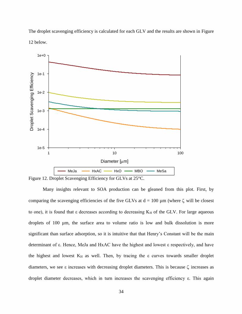
The droplet scavenging efficiency is calculated for each GLV and the results are shown in Figure

12 below.

Diameter [m]

1 10 100

Dro

ple

t S

cavengin

g E

ffic

iency

1e-5

1e-4

1e-3

1e-2

1e-1

1e+0

MeJa HxAC HxO MBO MeSa

Figure 12. Droplet Scavenging Efficiency for GLVs at 25°C.

Many insights relevant to SOA production can be gleaned from this plot. First, by

comparing the scavenging efficiencies of the five GLVs at d = 100 µm (where will be closest

to one), it is found that ε decreases according to decreasing KH of the GLV. For large aqueous

droplets of 100 µm, the surface area to volume ratio is low and bulk dissolution is more

significant than surface adsorption, so it is intuitive that that Henry’s Constant will be the main

determinant of ε. Hence, MeJa and HxAC have the highest and lowest ε respectively, and have

the highest and lowest KH as well. Then, by tracing the ε curves towards smaller droplet

diameters, we see ε increases with decreasing droplet diameters. This is because increases as

droplet diameter decreases, which in turn increases the scavenging efficiency ε. This again

35

makes logical sense: for the same aqueous volume, increasing the surface area available for

adsorption (by way of smaller droplet diameters) will result in more GLV being adsorbed to the

air-water interface at equilibrium. The difference between ε at diameter of 1 and 100 µm is

determined by the magnitude of the KSW term. For HxAC, the GLV with the largest KSW, this

difference is large, but for MBO, the GLV with the smallest KSW, the difference is minimal.

Overall, the plot clearly indicates the importance of MeJa in aqueous phase processing.

At droplet diameters of 1 µm, almost half of MeJa can be found in the surface or bulk aqueous

phases. Even at droplet diameter 50 µm where the surface phase is a negligible store for MeJa,

almost 7% of the total MeJa molecules reside in the droplet. For most of the other GLVs, the air-

water interface is a significant store, especially at small droplet sizes. Only MBO does not show

a significant variation due to droplet size, due to its low KSW.

This example can be used to elucidate the partitioning behavior of GLV molecules

between surface and bulk phases in the aqueous droplet alone. Consider only the mols on the

surface nS and the mols in the bulk nW. The ratio of nS to nW can be easily found by manipulating

the KSW definition as in Equation 6 below.

𝑛𝑆

𝑛𝑊=

𝐶𝑆∗𝐷𝑟𝑜𝑝𝑙𝑒𝑡 𝑆𝑢𝑟𝑓𝑎𝑐𝑒 𝐴𝑟𝑒𝑎

𝐶𝑊∗𝐷𝑟𝑜𝑝𝑙𝑒𝑡 𝑉𝑜𝑙𝑢𝑚𝑒= 𝐾𝑆𝑊 ∗

3

𝑟 Equation 6

Here r is the droplet radius. This gives the ratio of the number of mols on the droplet surface to

the number of mols in the droplet’s bulk, which is then used to find the percentage of the

individual droplet’s total mols (nS + nW) which can be found on the droplet’s surface. A plot

showing this percentage of the total number of mols in each aqueous droplet which reside on the

droplet’s surface as a function of droplet radius is shown Figure 13 below. For example, in the

case of HxAC, the molecule with the largest KSW, up to 80% of the GLV molecules are on the

surface for a water droplet of 2 µm radius. MBO, with the lowest KSW, has almost no GLV

36

residing in its surface phase. The calculation emphasizes that not only is the aqueous phase

significant for GLV scavenging, but that for fog-sized aqueous droplets, the air-water interface

can be a significant store for GLVs compared to the bulk phase.

Droplet radius [µm]

0 2 4 6 8 10 12 14

Perc

enta

ge o

f to

tal G

LV

in fog d

rople

tpart

itio

ned to s

urf

ace a

queous p

hase

0

20

40

60

80

100

HxAC

MBO

HxO

MeJa

MeSa

Figure 13. The percentage of GLV in the aqueous phase of a theoretical fog droplet which is

adsorbed to the air-water interface

37

CHAPTER 5

CONCLUSION

In this study, various physical properties of a class of biogenic volatile organic

compounds called green leaf volatiles have been determined. Experimental values of the Henry’s

Constant, aqueous solubility, and 1-octanol/water partition coefficient of five GLVs (Methyl

Jasmonate (MeJa), Methyl Salicylate (MeSa), 2-methyl-3-buten-2-ol (MBO), cis-3-hexen-1-ol

(HxO) and cis-3-hexenylacetate (HxAC)) were obtained. Estimation methods were also used to

predict each property which indicated that for oxygenated multifunctional compounds such as

GLVs, a bond contribution method is more accurate than a group contribution method for

predicting properties, but neither is recommended for complex, multifunctional compounds –

especially those with substituted aromatic groups. If an experimentally determined value for

either aqueous solubility or log(KOW) is available, it is preferable to use it to correlate the other

rather than using a “from scratch” method to estimate either. The effects on KH of temperature

and ionic strength relevant to natural fog water samples were found, yielding the enthalpy of

phase change for each GLV and showing that all but four GLVs underwent a salting-out effect in

the presence of aqueous phase ions. The surface to bulk aqueous and the air-surface partition

coefficient were determined from the physico-chemical thermodynamic properties. This

information was used in sample calculations to provide information on the partitioning

characteristics of various compounds in natural water samples of different types, and was used to

show that a sizable fraction of the GLV loading in an environmental fog droplet would be on the

surface for all GLVs except MBO. Additionally, the scavenging efficiency as a function of the

size of atmospheric water droplets can be obtained. From this, the amount of GLV in fog is

shown to be significant, especially for MeJa. This is relevant for any aqueous media with large

38

surface area to volume ratios such as clouds and fog, and emphasizes the importance of aqueous

phase photochemistry to fully elucidating SOA formation mechanisms. The physical properties

determined in this study can be used in further studies and atmospheric multiphase models to

determine the fate of GLVs in the atmosphere and their contribution to secondary organic aerosol

production from the aqueous phase.

39

REFERENCES

Abraham, M. H., J. Andonian-Haftvan, G. S. Whiting, A. Leo and R. S. Taft (1994).

"Hydrogen bonding. Part 34. The factors that influence the solubility of gases and

vapours in water at 298 K, and a new method for its determination." Journal of the

Chemical Society, Perkin Transactions 2(8): 1777-1791.

Arey, J., A. M. Winer, R. Atkinson, S. M. Aschmann, W. D. Long and C. L. Morrison

(1991). "The emission of (Z)-3-hexen-1-ol, (Z)-3-hexenylacetate and other

oxygenated hydrocarbons from agricultural plant species." Atmos. Environ., Part A

25A(5-6): 1063-1075.

Ashworth, R. A., G. B. Howe, M. E. Mullins and T. N. Rogers (1988). "Air-water

partitioning coefficients of organics in dilute aqueous solutions." Journal of

Hazardous Materials 18(1): 25-36.

Atkinson, R. (2000). "Atmospheric chemistry of VOCs and NOx." Atmos. Environ. 34(12-

14): 2063-2101.

Baev, A. K. (2012). Specific Intermolecular Interactions of Organic Compounds, Springer.

Bamford, H. A., D. L. Poster and J. E. Baker (1999). "Method for measuring the

temperature dependence of the Henry's Law Constant of selected polycyclic aromatic

hydrocarbons." Polycyclic Aromat. Compd. 14-15: 11-22.

Banerjee, S., S. H. Yalkowsky and C. Valvani (1980). "Water solubility and octanol/water

partition coefficients of organics. Limitations of the solubility-partition coefficient

correlation." Environ. Sci. Technol. 14(Copyright (C) 2014 American Chemical

Society (ACS). All Rights Reserved.): 1227-1229.

Blando, J. D. and B. J. Turpin (2000). "Secondary organic aerosol formation in cloud and

fog droplets: a literature evaluation of plausibility." Atmospheric Environment

34(10): 1623-1632.

Cabani, S., P. Gianni, V. Mollica and L. Lepori (1981). "Group contributions to the

thermodynamic properties of non-ionic organic solutes in dilute aqueous solution."

Journal of Solution Chemistry 10(8): 563-595.

Change, I. P. o. C. (2013). Contribution to the Fifth Assessment Report of the

Intergovernmental Panel on Climate Change. T. F. Stocker and D. Qin.

Chen, J., F. S. Ehrenhauser, K. T. Valsaraj and M. J. Wornat (2006). "Uptake and UV-

Photooxidation of Gas-Phase PAHs on the Surface of Atmospheric Water Films. 1.

Naphthalene." J. Phys. Chem. A 110(29): 9161-9168.

40

Chickos, J. S. and W. E. Acree (2003). "Enthalpies of Vaporization of Organic and

Organometallic Compounds, 1880–2002." Journal of Physical and Chemical

Reference Data 32(2): 519-878.

Chin, M., R. Kahn and S. E. Schwartz (2009). Atmospheric Aerosol Properties and Climate

Impacts., in U.S. Climate Change Science Program and the Subcommittee on Global

Change Research. M. Chin, NASA.

Chiou, C. T., V. H. Freed, D. W. Schmedding and R. L. Kohnert (1977). "Partition

coefficient and bioaccumulation of selected organic chemicals." Environ. Sci.

Technol. 11(Copyright (C) 2014 American Chemical Society (ACS). All Rights

Reserved.): 475-478.

Chiou, C. T., D. W. Schmedding and M. Manes (1982). "Partitioning of organic compounds

in octanol-water systems." Environ. Sci. Technol. 16(1): 4-10.

Cramer, R. D. (1980). "BC(DEF) parameters. 2. An empirical structure-based scheme for

the prediction of some physical properties." Journal of the American Chemical

Society 102(6): 1849-1859.

Dearden, J. C. and G. Schüürmann (2003). "Quantitative structure-property relationships for

predicting henry's law constant from molecular structure." Environmental

Toxicology and Chemistry 22(8): 1755-1770.

Dewulf, J., D. Drijvers and H. van Langenhove (1995). "Measurement of Henry's law

constant as function of temperature and salinity for the low temperature range."

Atmos. Environ. 29(3): 323-331.

EPA, U. from http://www.epa.gov/iaq/voc2.html.

EPA, U. (2012). Estimation Program Interface Suite. Washington, DC, US EPA.

Ervens, B., B. J. Turpin and R. J. Weber (2011). "Secondary organic aerosol formation in

cloud droplets and aqueous particles (aqSOA): a review of laboratory, field and

model studies." Atmos. Chem. Phys. 11(21): 11069-11102.

Facchini, M. C., S. Decesari, M. Mircea, S. Fuzzi and G. Loglio (2000). "Surface tension of

atmospheric wet aerosol and cloud/fog droplets in relation to their organic carbon

content and chemical composition." Atmospheric Environment 34(28): 4853-4857.

Falabella, J. B., A. Nair and A. S. Teja (2006). "Henry's Constants of 1-Alkanols and 2-

Ketones in Salt Solutions." Journal of Chemical & Engineering Data 51(5): 1940-

1945.

41

Farag, M. A. and P. W. Pare (2002). "C6-Green leaf volatiles trigger local and systemic

VOC emissions in tomato." Phytochemistry 61(5): 545-554.

Fowler, D., K. Pilegaard, M. A. Sutton, P. Ambus, M. Raivonen, J. Duyzer, D. Simpson, H.

Fagerli, S. Fuzzi, J. K. Schjoerring, C. Granier, A. Neftel, I. S. A. Isaksen, P. Laj, M.

Maione, P. S. Monks, J. Burkhardt, U. Daemmgen, J. Neirynck, E. Personne, R.

Wichink-Kruit, K. Butterbach-Bahl, C. Flechard, J. P. Tuovinen, M. Coyle, G.

Gerosa, B. Loubet, N. Altimir, L. Gruenhage, C. Ammann, S. Cieslik, E. Paoletti, T.

N. Mikkelsen, H. Ro-Poulsen, P. Cellier, J. N. Cape, L. Horvath, F. Loreto, U.

Niinemets, P. Palmer, J. Rinne, P. Misztal, E. Nemitz, D. Nilsson, S. Pryor, M. W.

Gallagher, T. Vesala, U. Skiba, N. Brueggemann, S. Zechmeister-Boltenstern, J.

Williams, C. O'Dowd, M. C. Facchini, G. de Leeuw, A. Flossman, N. Chaumerliac,

J. W. Erisman, D. Fowler, K. Pilegaard, M. A. Sutton, P. Ambus, M. Raivonen, J.

Duyzer, D. Simpson, H. Fagerli, S. Fuzzi, J. K. Schjoerring, C. Granier, A. Neftel, I.

S. A. Isaksen, P. Laj, M. Maione, P. S. Monks, J. Burkhardt, U. Daemmgen, J.

Neirynck, E. Personne, R. Wichink-Kruit, K. Butterbach-Bahl, C. Flechard, J. P.

Tuovinen, M. Coyle, G. Gerosa, B. Loubet, N. Altimir, L. Gruenhage, C. Ammann,

S. Cieslik, E. Paoletti, T. N. Mikkelsen, H. Ro-Poulsen, P. Cellier, J. N. Cape, L.

Horvath, F. Loreto, U. Niinemets, P. Palmer, J. Rinne, P. Misztal, E. Nemitz, D.

Nilsson, S. Pryor, M. W. Gallagher, T. Vesala, U. Skiba, N. Brueggemann, S.

Zechmeister-Boltenstern, J. Williams, C. O'Dowd, M. C. Facchini, G. de Leeuw, A.

Flossman, N. Chaumerliac and J. W. Erisman (2009). "Atmospheric composition

change: Ecosystems-Atmosphere interactions." Atmospheric Environment 43(33):

5193-5267.

Gelencser, A. (2005). Carbonaceous Aerosol. Dordrecht, The Netherlands, Springer.

Goldstein, A. H. and I. E. Galbally (2007). "Known and unexplored organic constituents in

the Earth's atmosphere." Environ. Sci. Technol. 41(5): 1514-1521.

Graedel, T. E. (1978). Chemical Compounds in the Atmosphere. New York, Academic

Press.

Graedel, T. E., Hawkins, D.T.; Claxton, L.D. (1986). Atmospheric Chemical Compounds.

Orlando, FL, Academic Press.

Guenther, A., C. N. Hewitt, D. Erickson, R. Fall, C. Geron, T. Graedel, P. Harley, L.

Klinger, M. Lerdau and a. et (1995). "A global model of natural volatile organic

compound emissions." J. Geophys. Res., [Atmos.] 100(D5): 8873-8892.

Hall, W. A. I. V. and M. V. Johnston (2010). "Oligomer content of α-pinene secondary

organic aerosol." Aerosol Sci. Technol. 45(1): 37-45.

Hallquist, M., J. C. Wenger, U. Baltensperger, Y. Rudich, D. Simpson, M. Claeys, J.

Dommen, N. M. Donahue, C. George, A. H. Goldstein, J. F. Hamilton, H. Herrmann,

T. Hoffmann, Y. Iinuma, M. Jang, M. E. Jenkin, J. L. Jimenez, A. Kiendler-Scharr,

42

W. Maenhaut, G. McFiggans, T. F. Mentel, A. Monod, A. S. H. Prévôt, J. H.

Seinfeld, J. D. Surratt, R. Szmigielski and J. Wildt (2009). "The formation,

properties and impact of secondary organic aerosol: current and emerging issues."

Atmos. Chem. Phys. 9(14): 5155-5236.

Hamilton, J. F., A. C. Lewis, T. J. Carey, J. C. Wenger, E. Borrais i Garcia and A. Munoz

(2009). "Reactive oxidation products promote secondary volatile organic aerosol

formation from green leaf volatiles." Atmospheric Chemistry and Physics 9: 3815-

3823.

Harley, P., V. Fridd-Stroud, J. Greenberg, A. Guenther and P. Vasconcellos (1998).

"Emission of 2-methyl-3-buten-2-ol by pines: A potentially large natural source of

reactive carbon to the atmosphere." Journal of Geophysical Research: Atmospheres

103(D19): 25479-25486.

Harvey, R. M., J. Zahardis and G. A. Petrucci (2014). "Establishing the contribution of lawn

mowing to atmospheric aerosol levels in American suburbs." Atmos. Chem. Phys.

14(2): 797-812.

Heiden, A. C., T. Hoffmann, J. Kahl, D. Kley, D. Klockow, C. Langebartels, H. Mehlhorn,

H. Sandermann, M. Schraudner, G. Schuh and J. Wildt (1999). "EMISSION OF

VOLATILE ORGANIC COMPOUNDS FROM OZONE-EXPOSED PLANTS."

Ecological Applications 9(4): 1160-1167.

Herckes, P., K. T. Valsaraj and J. L. Collett, Jr. (2013). "A review of observations of

organic matter in fogs and clouds: Origin, processing and fate." Atmos. Res. 132-

133: 434-449.

Hilal, S. H., S. W. Karickhoff and L. A. Carreira (2003). "Prediction of the vapor pressure,

boiling point, heat of vaporization and diffusion coefficient of organic compounds."

QSAR Comb. Sci. 22(Copyright (C) 2014 American Chemical Society (ACS). All

Rights Reserved.): 565-574.

Hine, J. and P. K. Mookerjee (1975). "Structural effects on rates and equilibriums. XIX.

Intrinsic hydrophilic character of organic compounds. Correlations in terms of

structural contributions." J. Org. Chem. 40(Copyright (C) 2014 American Chemical

Society (ACS). All Rights Reserved.): 292-298.

Ip, H. S. S., X. H. H. Huang and J. Z. Yu (2009). "Effective Henry's law constants of

glyoxal, glyoxylic acid, and glycolic acid." Geophys. Res. Lett. 36(1):

L01802/01801-L01802/01805.

Isnard, P. and S. Lambert (1989). "Aqueous solubility and n-octanol/water partition

coefficient correlations." Chemosphere 18(9-10): 1837-1853.

43

Jain, N., Y. Ran and S. H. Yalkowsky (2001). "Prediction of Aqueous Solubility of Organic

Compounds by the General Solubility Equation (GSE)." J. Chem. Inf. Comput. Sci.

41(Copyright (C) 2014 American Chemical Society (ACS). All Rights Reserved.):

1208-1217.

Jardine, K., L. Abrell, S. A. Kurc, T. Huxman, J. Ortega and A. Guenther (2010). "Volatile

organic compound emissions from Larrea tridentata (creosotebush)." Atmos. Chem.

Phys. 10(24): 12191-12206.

Kanakidou, M., J. H. Seinfeld, S. N. Pandis, I. Barnes, F. J. Dentener, M. C. Facchini, R.

Van Dingenen, B. Ervens, A. Nenes, C. J. Nielsen, E. Swietlicki, J. P. Putaud, Y.

Balkanski, S. Fuzzi, J. Horth, G. K. Moortgat, R. Winterhalter, C. E. L. Myhre, K.

Tsigaridis, E. Vignati, E. G. Stephanou and J. Wilson (2005). "Organic aerosol and

global climate modelling: a review." Atmos. Chem. Phys. 5(4): 1053-1123.

Karl, T., A. Guenther, A. Turnipseed, E. G. Patton and K. Jardine (2008). "Chemical

sensing of plant stress at the ecosystem scale." Biogeosciences 5: 1287-1294.

Karl, T., C. Yeretzian, A. Jordan and W. Lindinger (2003). "Dynamic measurements of

partition coefficients using proton-transfer-reaction mass spectrometry (PTR–MS)."

International Journal of Mass Spectrometry 223–224(0): 383-395.

Kesselmeier, J. and M. Staudt (1999). "Biogenic Volatile Organic Compounds (VOC): An

Overview on Emission, Physiology and Ecology." Journal of Atmospheric Chemistry

33(1): 23-88.

Kim, S., T. Karl, A. Guenther, G. Tyndall, J. Orlando, P. Harley, R. Rasmussen and E. Apel

(2010). "Emissions and ambient distributions of Biogenic Volatile Organic

Compounds (BVOC) in a ponderosa pine ecosystem: interpretation of PTR-MS mass

spectra." Atmos. Chem. Phys. 10(4): 1759-1771.

Kirstine, W., I. Galbally, Y. Ye and M. Hooper (1998). "Emissions of volatile organic

compounds (primarily oxygenated species) from pasture." J. Geophys. Res., [Atmos.]

103(D9): 10605-10619.

Liyana-Arachchi, T. P., A. K. Hansel, C. Stevens, F. S. Ehrenhauser, K. T. Valsaraj and F.

R. Hung (2013). "Molecular Modeling of the Green Leaf Volatile Methyl Salicylate

on Atmospheric Air/Water Interfaces." J. Phys. Chem. A 117(Copyright (C) 2014

American Chemical Society (ACS). All Rights Reserved.): 4436-4443.

Liyana-Arachchi, T. P., C. Stevens, A. K. Hansel, F. S. Ehrenhauser, K. T. Valsaraj and F.

R. Hung (2013). "Molecular simulations of green leaf volatiles and atmospheric

oxidants on air/water interfaces." Phys. Chem. Chem. Phys. 15(Copyright (C) 2014

American Chemical Society (ACS). All Rights Reserved.): 3583-3592.

44

Liyana-Arachchi, T. P., Z. Zhang, H. Vempati, A. K. Hansel, C. Stevens, A. T. Pham, F. S.

Ehrenhauser, K. T. Valsaraj and F. R. Hung (2014). "Green Leaf Volatiles on

Atmospheric Air/Water Interfaces: A Combined Experimental and Molecular

Simulation Study." Journal of Chemical & Engineering Data.

Liyana-Arachchi, T. P., Z. Zhang, H. Vempati, A. K. Hansel, C. Stevens, A. T. Pham, F. S.

Ehrenhauser, K. T. Valsaraj and F. R. Hung (2014). "Green Leaf Volatiles on

Atmospheric Air/Water Interfaces: A Combined Experimental and Molecular

Simulation Study." J. Chem. Eng. Data(Copyright (C) 2014 American Chemical

Society (ACS). All Rights Reserved.): Ahead of Print.

Mackay, D., W. Y. Shiu and R. P. Sutherland (1979). "Determination of air-water Henry's

law constants for hydrophobic pollutants." Environmental Science & Technology

13(3): 333-337.

Marrero, J. and R. Gani (2002). "Group-Contribution-Based Estimation of Octanol/Water

Partition Coefficient and Aqueous Solubility." Ind. Eng. Chem. Res. 41(Copyright

(C) 2014 American Chemical Society (ACS). All Rights Reserved.): 6623-6633.

Matsui, K. (2006). "Green leaf volatiles: hydroperoxide lyase pathway of oxylipin

metabolism." Current Opinion in Plant Biology 9(3): 274-280.

Mauderly, J. L. and J. C. Chow (2008). "Health Effects of Organic Aerosols." Inhalation

Toxicol. 20(3): 257-288.

Mentel, T. F., E. Kleist, S. Andres, M. Dal Maso, T. Hohaus, A. Kiendler-Scharr, Y.

Rudich, M. Springer, R. Tillmann, R. Uerlings, A. Wahner and J. Wildt (2013).

"Secondary aerosol formation from stress-induced biogenic emissions and possible

climate feedbacks." Atmos. Chem.Phys. 13: 8755-8770.

Meylan, W. M. and P. H. Howard (1991). "Bond contribution method for estimating henry's

law constants." Environmental Toxicology and Chemistry 10(10): 1283-1293.

Meylan, W. M. and P. H. Howard (1995). "Atom/Fragment Contribution Method for

Estimating Octanol-Water Partition Coefficients." J. Pharm. Sci. 84(1): 83-92.

Meylan, W. M. and P. H. Howard (1996). Sources and estimations of octanol-water partition

coefficients and water solubilities, Lewis.

Miller, M. M., S. P. Wasik, G. L. Huang, W. Y. Shiu and D. Mackay (1985). "Relationships

between octanol-water partition coefficient and aqueous solubility." Environmental

Science & Technology 19(6): 522-529.

Mmereki, B. T. and D. J. Donaldson (2003). "Direct observation of the kinetics of an

atmospherically important reaction at the air-aqueous interface." J. Phys. Chem. A

45

107(Copyright (C) 2014 American Chemical Society (ACS). All Rights Reserved.):

11038-11042.

Modarresi, H., H. Modarress and J. C. Dearden (2007). "QSPR model of Henry’s law

constant for a diverse set of organic chemicals based on genetic algorithm-radial

basis function network approach." Chemosphere 66(11): 2067-2076.

Morawetz, E. (1972). "Enthalpies of vaporization for a number of aromatic compounds."

The Journal of Chemical Thermodynamics 4(3): 455-460.

Munger, J. W., D. J. Jacob, J. M. Waldman and M. R. Hoffmann (1983). "Fogwater

chemistry in an urban atmosphere." JGR, J. Geophys. Res., [Sect.] C 88(C9): 5109-

5121.

Nirmalakhandan, N., R. A. Brennan and R. E. Speece (1997). "Predicting Henry's law

constant and the effect of temperature on Henry's law constant." Water Res.

31(Copyright (C) 2014 American Chemical Society (ACS). All Rights Reserved.):

1471-1481.

Preston, C. A., G. Laue and I. T. Baldwin (2001). "Methyl jasmonate is blowing in the wind,

but can it act as a plant–plant airborne signal?" Biochemical Systematics and

Ecology 29(10): 1007-1023.

Pruppacher, H. R. and R. Jaenicke (1995). "The processing of water vapor and aerosols by

atmospheric clouds, a global estimate." Atmospheric Research 38(1–4): 283-295.

Raja, S., R. Raghunathan, R. R. Kommalapati, X. Shen, J. L. Collett and K. T. Valsaraj

(2009). "Organic composition of fogwater in the Texas-Louisiana gulf coast

corridor." Atmos. Environ. 43(27): 4214-4222.

Raja, S., R. Ravikrishna, R. R. Kommalapati and K. T. Valsaraj (2005). "Monitoring of

fogwater chemistry in the gulf coast urban industrial corridor: Baton Rouge

(louisiana)." Environ Monit Assess 110(1-3): 99-120.

Richards-Henderson, N. K., A. K. Hansel, K. T. Valsaraj and C. Anastasio (2014).

"Aqueous oxidation of green leaf volatiles by hydroxyl radical as a source of SOA:

Kinetics and SOA yields." Atmos. Environ. 95: 105-112.

Robinson, A. L., N. M. Donahue, M. K. Shrivastava, E. A. Weitkamp, A. M. Sage, A. P.

Grieshop, T. E. Lane, J. R. Pierce and S. N. Pandis (2007). "Rethinking Organic

Aerosols: Semivolatile Emissions and Photochemical Aging." Science (Washington,

DC, U. S.) 315(5816): 1259-1262.

Russell, C. J., S. L. Dixon and P. C. Jurs (1992). "Computer-assisted study of the

relationship between molecular structure and Henry's law constant." Analytical

Chemistry 64(13): 1350-1355.

46

Schüürmann, G. (1995). "Quantum chemical approach to estimate physicochemical

compound properties: Application to substituted benzenes." Environmental

Toxicology and Chemistry 14(12): 2067-2076.

Seinfeld, J. H. and S. N. Pandis (1998). Atmospheric Chemistry and Physics: From Air

Pollution to Climate Change, Wiley.

Seinfeld, J. H., S. N. Pandis and Editors (2006). Atmospheric chemistry and physics: from

air pollution to climate change, 2nd Edition, Wiley.

Shiojiri, K., K. Kishimoto, R. Ozawa, S. Kugimiya, S. Urashimo, G. Arimura, J. Horiuchi,

T. Nishioka, K. Matsui and J. Takabayashi (2006). "Changing green leaf volatile

biosynthesis in plants: An approach for improving plant resistance against both

herbivores and pathogens." Proceedings of the National Academy of Sciences of the

United States of America 103(45): 16672-16676.

Staudinger, J. and P. V. Roberts (1996). "A critical review of Henry's law constants for

environmental applications." Crit. Rev. Environ. Sci. Technol. 26(Copyright (C)

2014 American Chemical Society (ACS). All Rights Reserved.): 205-297.

Suzuki, T., K. Ohtaguchi and K. Koide (1992). "Application of principal components

analysis to calculate Henry's constant from molecular structure." Comput. Chem.

16(Copyright (C) 2014 American Chemical Society (ACS). All Rights Reserved.):

41-52.

Tewari, Y. B., M. M. Miller, S. P. Wasik and D. E. Martire (1982). "Aqueous solubility and

octanol/water partition coefficient of organic compounds at 25.0°C." J. Chem. Eng.

Data 27(Copyright (C) 2014 American Chemical Society (ACS). All Rights

Reserved.): 451-454.

Torres-Gómez, L. A., G. Barreiro-Rodríguez and A. Galarza-Mondragón (1988). "A new

method for the measurement of enthalpies of sublimation using differential scanning

calorimetry." Thermochimica Acta 124(0): 229-233.

Valsaraj, K. T. (2004). "Adsorption of polycyclic aromatic hydrocarbons at the air -water

interface and its role in atmospheric deposition by fog droplets." Environ Toxicol

Chem 23(10): 2318-2323.

Valsaraj, K. T. (2009). Elements of environmental engineering : thermodynamics and

kinetics. Boca Raton, CRC Press.

Valsaraj, K. T. (2012). "A review of the aqueous aerosol surface chemistry in the

atmospheric context." Open J. Phys. Chem. 2(1): 58-66.

Volkamer, R., J. L. Jimenez, F. San Martini, K. Dzepina, Q. Zhang, D. Salcedo, L. T.

Molina, D. R. Worsnop and M. J. Molina (2006). "Secondary organic aerosol

47

formation from anthropogenic air pollution: rapid and higher than expected."

Geophys. Res. Lett. 33(17): L17811/17811-L17811/17814.

Wadia, Y., D. J. Tobias, R. Stafford and B. J. Finlayson-Pitts (2000). "Real-Time

Monitoring of the Kinetics and Gas-Phase Products of the Reaction of Ozone with an

Unsaturated Phospholipid at the Air-Water Interface." Langmuir 16(Copyright (C)

2014 American Chemical Society (ACS). All Rights Reserved.): 9321-9330.

Williams, J., U. Pöschl, P. J. Crutzen, A. Hansel, R. Holzinger, C. Warneke, W. Lindinger

and J. Lelieveld (2001). "An Atmospheric Chemistry Interpretation of Mass Scans

Obtained from a Proton Transfer Mass Spectrometer Flown over the Tropical

Rainforest of Surinam." Journal of Atmospheric Chemistry 38(2): 133-166.

48

APPENDIX

Appendix A. Derivation of Thermodynamic Equations

The Henry’s Constant of a compound can be defined in varying units, here it is defined as

KH = CW/P [=] [M/atm], where CW is the analyte’s concentration in the aqueous phase, and P is

its partial pressure in the gas phase. It was originally an empirical result reflecting the

observation that amount gas dissolved in a liquid at equilibrium is proportional to its partial

pressure in equilibrium. In order to understand the use and potential estimations of Henry’s

Constant, solubility, and log(KOW) it is important to have some thermodynamic background. In

mixed solutions at equilibrium with air above it, the fugacity 𝑓 of an analyte in each phase are

equal.

𝑓𝐺 = 𝑓𝐿 (7)

Here 𝑓𝐺 is the analyte’s fugacity in the gas phase and 𝑓𝐿 is its fugacity in the liquid phase. If

ideality in the gas phase is assumed then 𝑓𝐺 is equal to the analyte’s partial pressure P and

Equation 7 can be expanded to Equation 8.

𝑃 = 𝑓𝐿 ∗ 𝛾𝐿 ∗ 𝑥𝐿 (8)

Here 𝑓𝐿 is the reference liquid fugacity, 𝛾𝐿 is the analyte fugacity in the liquid phase, and 𝑥𝐿 is

the anlyte’s liquid phase mol fraction. If we substitute the relation 𝑥𝐿 = 𝐶𝐿 ∗ ��𝐿 where ��𝐿 is the

molar volume of the solution and 𝐶𝐿 is the analyte’s concentration in it. By using Henry’s Law

conventions (as 𝐶𝐿 goes to zero, 𝛾𝐿 becomes 1), and if the solution is assumed sufficiently dilute

then this allows us to write:

lim𝐶𝐿 →0

(𝑃

𝐶𝐿) = 𝑓𝐿 ∗ 𝛾𝐿 ∗ ��𝐿 = 𝐾𝐻 (9)

If the liquid is taken to be water, this is the definition of Henry’s Law, and the one I will be using

in this work.

49

The saturated aqueous solubility of an analyte can likewise be expressed in fugacity terms by

equating the fugacity of the compound in its pure state with that of the compound in a saturated

aqueous state. This is shown below:

𝑓𝑃 ∗ 𝛾𝑃 ∗ 𝑥𝑃 = 𝑓𝑃 ∗ 𝛾𝑊 ∗ 𝑥𝑊 (10)

where the subscript P stands for the pure component state and W for the aqueous state. The

reference liquid state is taken to be the pure liquid solute, and these pure component fugacities

cancel out. Additionally for the pure component phase 𝛾𝑃 = 𝑥𝑃 = 1, and by substituting 𝑥𝑊 =

𝐶𝑊 ∗ ��𝑊 we find the final relation.

𝛾𝑊 = (𝐶𝑊 ∗ ��𝑊)−1 = (𝑆 ∗ ��𝑊)−1 (11)

Equation 9 states that the activity coefficient for an analyte in a saturated aqueous solution is

inversely proportional to its saturated aqueous concentration.

The octanol-water partitioning of an analyte can also be expressed in terms of fugacity. In

an octanol-water system at equilibrium, the fugacity of the analyte in the octanol phase

(designated by subscript O) is equal to the fugacity of the analyte in the aqueous phase

(designated by subscript W), and if the reference fugacity is again that of the pure component

liquid, we find Equation 12.

𝑓𝑃 ∗ 𝛾𝑂 ∗ 𝑥𝑂 = 𝑓𝑃 ∗ 𝛾𝑊 ∗ 𝑥𝑊 (12)

The pure component reference fugacity values again cancel, and if one substitutes 𝑥𝑂 = 𝐶𝑂 ∗ ��𝑂,

then by using the definition of octanol-water partition coefficient KOW = CO/CW, Equation 13 is

found.

𝐾𝑂𝑊 =𝐶𝑂

𝐶𝑊=

𝛾𝑊∗ ��𝑊

𝛾𝑂∗ ��𝑂 (13)

50

This can be correlated to the aqueous solubility of an analyte by substituting in the 𝛾𝑤 relation

found in Equation 8. This gives the result that KOW is proportional to inverse of the aqueous

solubility, which by taking the logarithm can also be expressed:

log 𝐾𝑂𝑊 = − log 𝑆 – log(𝛾𝑂 ∗ ��𝑂) (14)

Thus a linear relationship between log(KOW) and log(S) with slope -1 is found. However, this

neglects the fact that the solvents are not pure octanol and pure water, but are well mixed at

equilibrium and thus are mutually saturated. These changes are reflected in Equation 15, the

expression for KOW.

𝐾𝑜𝑤 =𝐶𝑜

𝐶𝑤 =𝛾��∗ ��𝑊

∗

𝛾��∗ ��𝑂∗ (15)

Here 𝛾�� and 𝛾�� are the compound’s activity coefficient in mutually saturated water and octanol

respectively. ��𝑊∗ and ��𝑂

∗ are the molar volume for the mutually saturated water and octanol

phases respectively. ��𝑊∗ is approximately equal to ��𝑊 (Miller et al. 1985), allowing combination

with Equation 9. This eventually leads to Equation 14.

log 𝐾𝑂𝑊 = − log 𝑆 + log 𝛾�� – log(𝛾�� ∗ 𝛾�� ∗ ��𝑂∗) (16)

These relationships form the thermodynamic basis of the log(KOW) vs log(S) correlation.

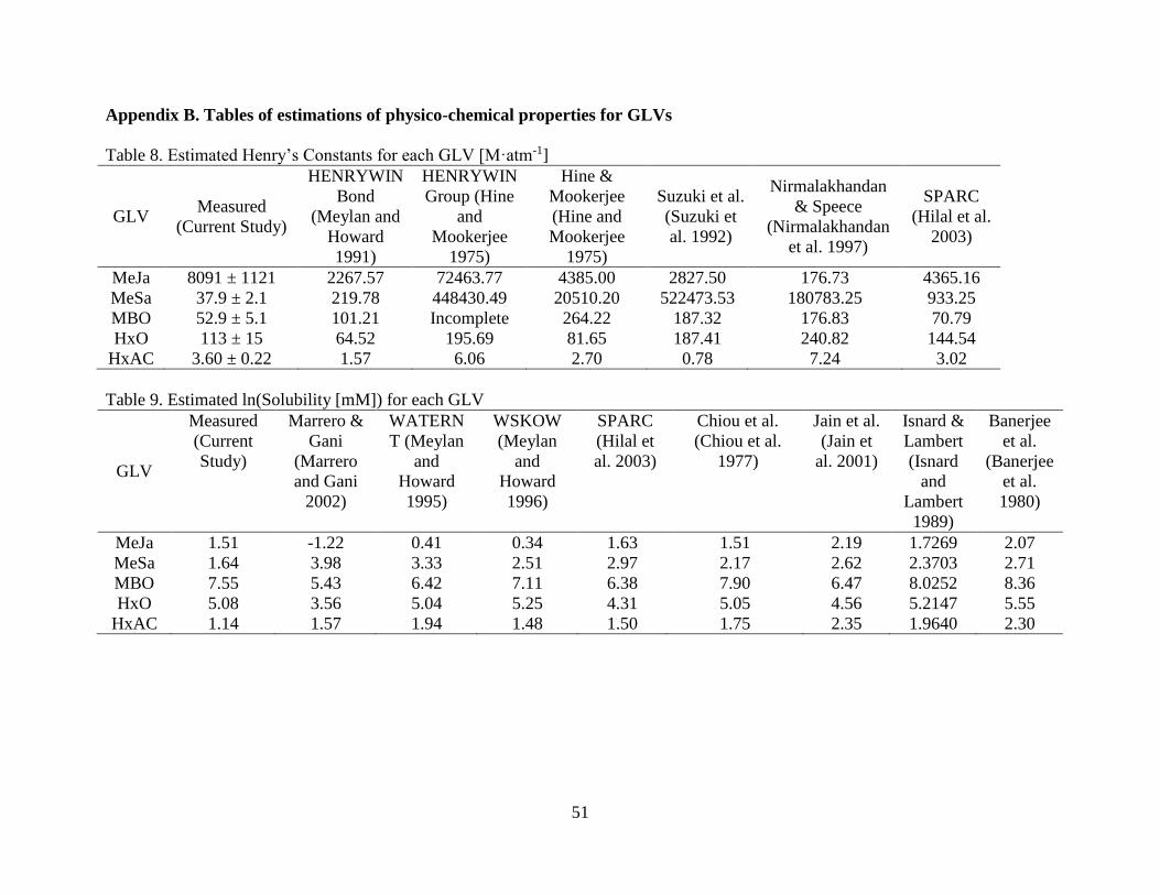
51

Appendix B. Tables of estimations of physico-chemical properties for GLVs

Table 8. Estimated Henry’s Constants for each GLV [M·atm-1]

GLV Measured

(Current Study)

HENRYWIN

Bond

(Meylan and

Howard

1991)

HENRYWIN

Group (Hine

and

Mookerjee

1975)

Hine &

Mookerjee

(Hine and

Mookerjee

1975)

Suzuki et al.

(Suzuki et

al. 1992)

Nirmalakhandan

& Speece

(Nirmalakhandan

et al. 1997)

SPARC

(Hilal et al.

2003)

MeJa 8091 ± 1121 2267.57 72463.77 4385.00 2827.50 176.73 4365.16

MeSa 37.9 ± 2.1 219.78 448430.49 20510.20 522473.53 180783.25 933.25

MBO 52.9 ± 5.1 101.21 Incomplete 264.22 187.32 176.83 70.79

HxO 113 ± 15 64.52 195.69 81.65 187.41 240.82 144.54

HxAC 3.60 ± 0.22 1.57 6.06 2.70 0.78 7.24 3.02

Table 9. Estimated ln(Solubility [mM]) for each GLV

GLV

Measured

(Current

Study)

Marrero &

Gani

(Marrero

and Gani

2002)

WATERN

T (Meylan

and

Howard

1995)

WSKOW

(Meylan

and

Howard

1996)

SPARC

(Hilal et

al. 2003)

Chiou et al.

(Chiou et al.

1977)

Jain et al.

(Jain et

al. 2001)

Isnard &

Lambert

(Isnard

and

Lambert

1989)

Banerjee

et al.

(Banerjee

et al.

1980)

MeJa 1.51 -1.22 0.41 0.34 1.63 1.51 2.19 1.7269 2.07

MeSa 1.64 3.98 3.33 2.51 2.97 2.17 2.62 2.3703 2.71

MBO 7.55 5.43 6.42 7.11 6.38 7.90 6.47 8.0252 8.36

HxO 5.08 3.56 5.04 5.25 4.31 5.05 4.56 5.2147 5.55

HxAC 1.14 1.57 1.94 1.48 1.50 1.75 2.35 1.9640 2.30

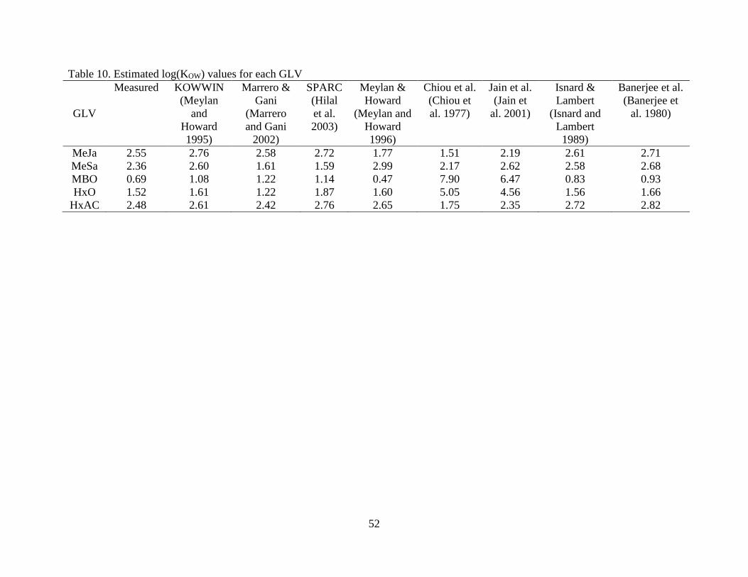
52

Table 10. Estimated log(KOW) values for each GLV

GLV

Measured KOWWIN

(Meylan

and

Howard

1995)

Marrero &

Gani

(Marrero

and Gani

2002)

SPARC

(Hilal

et al.

2003)

Meylan &

Howard

(Meylan and

Howard

1996)

Chiou et al.

(Chiou et

al. 1977)

Jain et al.

(Jain et

al. 2001)

Isnard &

Lambert

(Isnard and

Lambert

1989)

Banerjee et al.

(Banerjee et

al. 1980)

MeJa 2.55 2.76 2.58 2.72 1.77 1.51 2.19 2.61 2.71

MeSa 2.36 2.60 1.61 1.59 2.99 2.17 2.62 2.58 2.68

MBO 0.69 1.08 1.22 1.14 0.47 7.90 6.47 0.83 0.93

HxO 1.52 1.61 1.22 1.87 1.60 5.05 4.56 1.56 1.66

HxAC 2.48 2.61 2.42 2.76 2.65 1.75 2.35 2.72 2.82

53

VITA

Harsha Satyanarayana Vempati was raised in Chandler, Arizona and graduated from

Corona del Sol High School in 2008. Afterwards, he moved to Atlanta, Georgia and received his

bachelor’s degree at the Georgia Institute of Technology in 2012. He was interested in

environmental sciences, and upon acceptance into Louisiana State University’s Cain Department

of Chemical Engineering, joined the chemodynamics laboratory. He will receive his degree in

December 2014, and upon completion plans to work as an environmental consultant.