Embed Size (px)
Citation preview

Project FI4P-CT95-0021a ( PL 950128 )co-funded by the Nuclear Fission Safety Programme of the European Commission
Physico-Chemical Phenomena Governingthe Behaviour of Radioactive Substances.
State-of-the-Ar t Descr iption
Restoration Strategies for Radioactively Contaminated Sites and their Close Surroundings
RESTRAT - WP2
Vinzenz BrendlerForschungszentrum Rossendorf, Institute of Radiochemistry
P.O.Box. 51 01 19, D-01314 Dresden, Germany
RESTRAT-TD.2
18 August 1999 - Issue 4

RESTRAT - Physico-Chemical Phenomena: State-of-the-Art Description
18 August 1999 i Issue 4
Summary
Work package WP2.1 of the EC project RESTRAT characterizes the main parameters, namely physico-chemical ones, determining the source term evolution in radioactively contaminated sites with regard totheir importance and availability for risk assessment models, ensuring a more profound chemical base forrestoration scenarios.
This report summarizes the physico-chemical phenomena and their main parameters. It points out the waysto get the available data from sources like databases, scientific publications, or own experimentaldeterminations and measurements. Such a database establishment for each site to be remediated has to beaccompanied by an integration of chemical speciation into existing risk assessment codes. Therefore thestate-of-the-art of chemical speciation and migration modelling is described, leading to the conclusion thatit is necessary to unfold the wide-spread K -concept. K values have generally both large uncertainties andd d
important effects on the risk assessment predictions, particularly as models are often sensitive towardschanges in K . Hence an unfolding makes it possible to perform more detailed sensitivity analysis, to findd
the most critical parameters, to reduce parameter space, and finally to prepare the way for more reliablemodels.
Consequently, the models for surface complexation most often used in geochemical modelling arepresented here. For both non-electrostatic and electrostatic adsorption models the defining equations,theoretical background and the main parameters are given. Because surface complexation models, togetherwith chemical speciation, are to be combined with currently used risk assessment software, theimplementation of such surface complexation models in the geochemical code MINTEQA2 [Allison et al.,1991] is explained.
In its last part, this work describes data structures and data flows for the proposed strategy of a Kd
unfolding, namely the combination of MINTEQA2 with the PRISM / BIOPATH [Gardner et al., 1983;Bergström et al., 1982] package.
It is hoped that the work performed under the RESTRAT project, and especially the part presented in thisreport, will help to define and use a common language among all the different group of scientists, involvedand required in such a true multi-disciplinary and complex challenge as the risk assessment forradioactively contaminated sites.

RESTRAT - Physico-Chemical Phenomena: State-of-the-Art Description
18 August 1999 ii Issue 4
Table of Contents
1. Introduction . . . . . . . . . . . . . . . . . . . . . . . . . . . . . . . . . . . . . . . . . . . . . . . . . . . . . . . . . . . . . . . . . . . . 1
2. Important physico-chemical processes . . . . . . . . . . . . . . . . . . . . . . . . . . . . . . . . . . . . . . . . . . . . . . . . 2
3. Physico-chemical parameters necessary to describe natural systems . . . . . . . . . . . . . . . . . . . . . . . . . 33.1. Site-specific parameters . . . . . . . . . . . . . . . . . . . . . . . . . . . . . . . . . . . . . . . . . . . . . . . . . . . . . . 3
3.1.1. Description of the stationary state ( composition ) of a system . . . . . . . . . . . . . . . . . . . . 33.1.2. Description of the system´s evolution in time and space . . . . . . . . . . . . . . . . . . . . . . . . . 4
3.2. Reaction-specific ( system independent ) parameters . . . . . . . . . . . . . . . . . . . . . . . . . . . . . . . . 4
4. Database establishment . . . . . . . . . . . . . . . . . . . . . . . . . . . . . . . . . . . . . . . . . . . . . . . . . . . . . . . . . . . 54.1. Problems with the determination of site-specific parameters . . . . . . . . . . . . . . . . . . . . . . . . . . 54.2. Sampling recommendations . . . . . . . . . . . . . . . . . . . . . . . . . . . . . . . . . . . . . . . . . . . . . . . . . . . 5
4.2.1. Quantitative analysis for anions and cations in aqueous solutions . . . . . . . . . . . . . . . . . 64.2.2. pH . . . . . . . . . . . . . . . . . . . . . . . . . . . . . . . . . . . . . . . . . . . . . . . . . . . . . . . . . . . . . . . . . . 64.2.3. Gas phase composition . . . . . . . . . . . . . . . . . . . . . . . . . . . . . . . . . . . . . . . . . . . . . . . . . . 74.2.4. Temperature . . . . . . . . . . . . . . . . . . . . . . . . . . . . . . . . . . . . . . . . . . . . . . . . . . . . . . . . . . 74.2.5. Redox state . . . . . . . . . . . . . . . . . . . . . . . . . . . . . . . . . . . . . . . . . . . . . . . . . . . . . . . . . . . 74.2.6. Organics . . . . . . . . . . . . . . . . . . . . . . . . . . . . . . . . . . . . . . . . . . . . . . . . . . . . . . . . . . . . . 74.2.7. Qualitative analysis of solid phases / minerals . . . . . . . . . . . . . . . . . . . . . . . . . . . . . . . . 74.2.8. Size distribution of dispersed or colloidal material . . . . . . . . . . . . . . . . . . . . . . . . . . . . . 8
4.3. Database situation for reaction specific parameters . . . . . . . . . . . . . . . . . . . . . . . . . . . . . . . . . 8
5. State-of-the-art chemical modelling . . . . . . . . . . . . . . . . . . . . . . . . . . . . . . . . . . . . . . . . . . . . . . . . . . 95.1. Terms and definitions . . . . . . . . . . . . . . . . . . . . . . . . . . . . . . . . . . . . . . . . . . . . . . . . . . . . . . . . 95.2. Defining a chemical system . . . . . . . . . . . . . . . . . . . . . . . . . . . . . . . . . . . . . . . . . . . . . . . . . . . 95.3. Mathematical formulation . . . . . . . . . . . . . . . . . . . . . . . . . . . . . . . . . . . . . . . . . . . . . . . . . . . . 105.4. Migration modelling . . . . . . . . . . . . . . . . . . . . . . . . . . . . . . . . . . . . . . . . . . . . . . . . . . . . . . . . 115.5. Available speciation and migration software . . . . . . . . . . . . . . . . . . . . . . . . . . . . . . . . . . . . . 12
5.5.1. Programs to compute speciations with given thermodynamic parameters . . . . . . . . . . . 125.5.2. Programs combining speciation modules with a transport code . . . . . . . . . . . . . . . . . . 135.5.3. Programs to iterate thermodynamic and/or kinetic parameters . . . . . . . . . . . . . . . . . . . 14
5.6. Criteria to select appropriate modelling software . . . . . . . . . . . . . . . . . . . . . . . . . . . . . . . . . . 15
6. Description of PRISM / BIOPATH . . . . . . . . . . . . . . . . . . . . . . . . . . . . . . . . . . . . . . . . . . . . . . . . . 16
7. Unfolding the K value . . . . . . . . . . . . . . . . . . . . . . . . . . . . . . . . . . . . . . . . . . . . . . . . . . . . . . . . . . . 17d
7.1. Why are the K values not satisfactory ? . . . . . . . . . . . . . . . . . . . . . . . . . . . . . . . . . . . . . . . . . 17d
7.2. Guidelines for unfolding the K . . . . . . . . . . . . . . . . . . . . . . . . . . . . . . . . . . . . . . . . . . . . . . . 17d
7.3. Selection of speciation programs . . . . . . . . . . . . . . . . . . . . . . . . . . . . . . . . . . . . . . . . . . . . . . 18
8. Models to describe sorption phenomena . . . . . . . . . . . . . . . . . . . . . . . . . . . . . . . . . . . . . . . . . . . . . 208.1. Non-electrostatic adsorption models . . . . . . . . . . . . . . . . . . . . . . . . . . . . . . . . . . . . . . . . . . . . 20
8.1.1. Distribution coefficient (K ) model . . . . . . . . . . . . . . . . . . . . . . . . . . . . . . . . . . . . . . . . 20d
8.1.2. Langmuir adsorption model . . . . . . . . . . . . . . . . . . . . . . . . . . . . . . . . . . . . . . . . . . . . . 218.1.3. Freundlich adsorption model . . . . . . . . . . . . . . . . . . . . . . . . . . . . . . . . . . . . . . . . . . . . . 21

RESTRAT - Physico-Chemical Phenomena: State-of-the-Art Description
18 August 1999 iii Issue 4
8.1.4. Ion exchange model . . . . . . . . . . . . . . . . . . . . . . . . . . . . . . . . . . . . . . . . . . . . . . . . . . . . 228.2. Electrostatic adsorption models . . . . . . . . . . . . . . . . . . . . . . . . . . . . . . . . . . . . . . . . . . . . . . . 22
8.2.1. Constant capacitance model . . . . . . . . . . . . . . . . . . . . . . . . . . . . . . . . . . . . . . . . . . . . . 238.2.2. Diffuse double layer model . . . . . . . . . . . . . . . . . . . . . . . . . . . . . . . . . . . . . . . . . . . . . . 238.2.3. Triple layer model . . . . . . . . . . . . . . . . . . . . . . . . . . . . . . . . . . . . . . . . . . . . . . . . . . . . . 23
8.3. Implementation of sorption models in the MINTEQA2 software . . . . . . . . . . . . . . . . . . . . . . 24
9. Combination of MINTEQA2 with PRISM and BIOPATH . . . . . . . . . . . . . . . . . . . . . . . . . . . . . . . 279.1. Chemical data input: internal structure and handling . . . . . . . . . . . . . . . . . . . . . . . . . . . . . . . 279.2. Application scheme . . . . . . . . . . . . . . . . . . . . . . . . . . . . . . . . . . . . . . . . . . . . . . . . . . . . . . . . 279.3. Description of data structures . . . . . . . . . . . . . . . . . . . . . . . . . . . . . . . . . . . . . . . . . . . . . . . . . 29
9.3.1. Chemical model description file ( model.chem ) . . . . . . . . . . . . . . . . . . . . . . . . . . . . . . 299.3.2. Conventional PRISM / BIOPATH input file ( model.box ) . . . . . . . . . . . . . . . . . . . . . 329.3.3. Template file for the chemical speciation ( minteq.template ) . . . . . . . . . . . . . . . . . . . . 329.3.4. Input file for PRISM2 ( PRISM2.INP ) . . . . . . . . . . . . . . . . . . . . . . . . . . . . . . . . . . . . . . . 329.3.5. Input file for PRISM3 ( PRISM3.INP ) . . . . . . . . . . . . . . . . . . . . . . . . . . . . . . . . . . . . . . . 33
9.4. Data flow between PRISM, BIOPATH and MINTEQA2 . . . . . . . . . . . . . . . . . . . . . . . . . . . 33
10. Conclusions . . . . . . . . . . . . . . . . . . . . . . . . . . . . . . . . . . . . . . . . . . . . . . . . . . . . . . . . . . . . . . . . . . 35
11. References . . . . . . . . . . . . . . . . . . . . . . . . . . . . . . . . . . . . . . . . . . . . . . . . . . . . . . . . . . . . . . . . . . . 36
12. Acknowledgment . . . . . . . . . . . . . . . . . . . . . . . . . . . . . . . . . . . . . . . . . . . . . . . . . . . . . . . . . . . . . . 44

RESTRAT - Physico-Chemical Phenomena: State-of-the-Art Description
18 August 1999 iv Issue 4
List of Tables and Figures
Table 1: Anions and cations to be analysed in aqueous solutions . . . . . . . . . . . . . . . . . . . . . . . . . . . 6Table 2: Chemical system set-up: master species for an aqueous solution of uranyl phosphate in contact
with the atmosphere . . . . . . . . . . . . . . . . . . . . . . . . . . . . . . . . . . . . . . . . . . . . . . . . . . . . . 10Table 3: Comparison of features of some programs modelling speciation and reactive transport . . 14
Figure 1: Data flow between preprocessor, PRISM, BIOPATH, MINTEQA2, and the interface modules. . . . . . . . . . . . . . . . . . . . . . . . . . . . . . . . . . . . . . . . . . . . . . . . . . . . . . . . . . . . . . . . . . . . . 34

RESTRAT - Physico-Chemical Phenomena: State-of-the-Art Description
18 August 1999 v Issue 4
List of Appendices
Appendix A: Example for an input file model.chem . . . . . . . . . . . . . . . . . . . . . . . . . . . . . . . . . . . . 45Appendix B: Example for a model.box input file . . . . . . . . . . . . . . . . . . . . . . . . . . . . . . . . . . . . . . 46Appendix C: Example for a MINTEQA2 input template . . . . . . . . . . . . . . . . . . . . . . . . . . . . . . . . 47
RESTRAT - Physico-Chemical Phenomena: State-of-the-Art Description
18 August 1999 1 Issue 4
1. Introduction
The main objective of the overall RESTRAT project is to develop a generic methodology for the rankingof restoration techniques as a function of site and contamination characteristics. The work has been brokendown into several work packages. This technical deliverable, as required by the contract, summarizes thework performed in work package WP 2: Physico-chemical phenomena during Phase 1: State-of-the-artdescription.
The focus is on the characterization of the main parameters, namely physico-chemical ones, determiningthe source term evolution with regard to their importance and availability for risk assessment models. Theaim is to deliver a more profound chemical base for risk assessment scenarios, which is accompanied bya general improvement of the communication and mutual understanding between risk assessmentresearchers and physico-chemists. In order to take properly into account the physico-chemical phenomenagoverning the contamination source term development in time and space, it is necessary to extend theknowledge about these phenomena and the underlying basic processes and interactions. This allows abetter integration of chemical speciation into existing risk assessment codes.
Up to now, the physico-chemical phenomena were considered ( if at all ) by applying distributioncoefficients (K ) in order to model the distribution of a contaminant between solid and aqueous phases.d
Such distribution coefficients generally have large uncertainties. In many cases sensitivity analysis for riskassessments revealed, that the uncertainty of the K was propagated throughout the whole model, contrib-d
uting to a large extent to the overall uncertainty of a prediction. In other words, risk assessment models areparticularly sensitive towards changes in K . To overcome this problem, strategies are required to “unfold”d
the K approach into more basic processes. This should make it possible to perform more detailedd
sensitivity analysis, to find the most critical parameters, to reduce parameter space and, finally, to pave theway to more reliable models.

RESTRAT - Physico-Chemical Phenomena: State-of-the-Art Description
simple ions or neutral molecules, ion pairs, associates, complexes, hydrolysis products, pure minerals, solid1
solutions, gases, surface complexes
aqueous solution in contact with all solid phases and the gas phase, maybe also other fluid phases (organics),2
colloids and aerosols
18 August 1999 2 Issue 4
2. Important physico-chemical processes
A contaminant can occur in many different forms in an environmental compartment, each of them havingdifferent mobility, transfer coefficients to and between living matter, and even toxicity. This variety ofexisting forms for a given element is termed chemical speciation, defined as the distribution of one or moreelements between all its possible species ( distinct chemical entities ) in a given system . It should be1 2
noted that the term “speciation” is also used in another context to describe all the experimental methodsapplied to investigate the above discussed species distribution.
Species distributions determine whether a contaminant is mainly a component - and thus easily transportedand taken up - or is immobilized through precipitation or adsorption onto a surface. Therefore, changes inspeciation can either accelerate or slow down radionuclide migration. Many of the processes affecting thesource term are influenced by the speciation. Their importance may vary, so the following list should notbe considered a ranking:- radioactive decay;- complexation reactions ( with organic and inorganic ligands ), through:
• hydrolysis;• dissociation;• association / polymerization;
- oxidation state changes / redox reactions;- precipitation and dissolution of solid phases;- co-precipitation ( inclusion & surface precipitation ) of trace components;- physical and chemical sorption onto mineral surfaces or colloids;- formation of solid solutions ( mixed mineral phases );- ion exchange;- extraction ( in case of several fluid phases );- formation of colloids;- formation of aerosols;- processes involving biological material, such as biosorption, biologically catalysed redox reactions,
enzymatic reactions, metabolisms.
Many of these processes are controlled by parameters from outside, which can be considered as fixed bycertain environmental ( natural and man-made ) conditions. But for some of these parameters feedback canbe observed; the internal physico-chemical processes of an environmental compartment will influenceparameters such as pH or redox potential, either amplifying or extenuating already established trends fromoutside the compartment. Without a thorough description of all parameters and processes, leading to acomprehensive, “ full-system” modelling, no sound prognostics are possible.

RESTRAT - Physico-Chemical Phenomena: State-of-the-Art Description
18 August 1999 3 Issue 4
3. Physico-chemical parametersnecessary to descr ibenatural systems
The various processes listed above can be described quantitatively by their respective functional terms,each requiring a unique set of parameters. Fortunately, many parameters are used simultaneously for manyor all of the above reactions, like temperature or concentrations. In general, the parameters can be dividedinto system-specific parameters ( subdivided into the stationary state and the dynamic evolution ) and intoreaction-specific parameters. Many of these parameters also depend on the chemical or physical modelsapplied to the system. The most obvious case is the number and kind of species thought to be present inthe system of interest, i.e. the selected speciation model [Appelo and Postma, 1993; Manahan, 1994; Ureand Davidson, 1995]. When the ionic strength I of the system exceeds the validity range of the Debye-Hückel Limiting Law, one has the choice between various activity coefficient models, such as the DaviesEquation [Davies, 1962], the Specific Ion Interaction Theory / SIT or Brønsted-Guggenheim-ScatchardModel [Grenthe et al.,1997], the Pitzer Model [Pitzer, 1973; Pitzer, 1991], the Mean SphericalApproximation ( MSA ) [Blum, 1988], and the models from Scatchard or Lim [Scatchard, 1968; Lim,1987]. The next step of complexity is added with the introduction of a Surface Complexation Model( SCM ) [Stumm, 1992]. Constant-Capacitance, Diffuse-Layer, Stern, Triple-Layer, Four-Layer-Model:all require their special set of parameters. In the case of mixed fluid phases one has to choose betweenmixing models such as Flory/Huggins, NRTL, UNIFAC, Wilson, van Laar, UNIQUAC, and ASOG.Kinetic rate laws or the models for the formation and interaction of colloids or aerosols also have their ownset of parameters [Connors, 1990; Schmalzried, 1995]. The thermodynamics of water and aqueoussolutions are dealt with in detail by various papers [Horne, 1971; Stumm and Morgan, 1996; Deutsch,1997].
3.1. Site-specific parameters
The parameters described below are all specific to a given site and must be determined by field studies orfrom samples in the laboratory ( see also Chapter 4 ). They either define the stationary state of a system orits dynamic evolution.
3.1.1. Descr iption of the stationary state ( composition ) of a system
- Temperature.- Pressure (total system and partial pressure of all gaseous components).- Elementary composition, concentrations for all components (total or, better, for each species sepa-
rately):• This includes pH , ionic strength , humidity.
- Composition of solid phases:• Identification of rocks and their mineral matrix.
- Redox state:• Eh, oxygen partial pressure, potentials of important redox pairs.
- Surface properties:• Specific surface area, active sites, site densities, crystal size, structural disorders, charge distribu-
tion, surface films ( biological matter! ).- Total water content.

RESTRAT - Physico-Chemical Phenomena: State-of-the-Art Description
18 August 1999 4 Issue 4
3.1.2. Descr iption of the system´s evolution in time and space
The parameters describing the temporal and spatial evolution of a system come from several disciplines,including chemistry, biology, hydrodynamics, meteorology, and geophysics. Therefore, this list is ratherheterogeneous.- Flow rates.- Geometries of flow paths.- Porosity of geomatrix.- Gradients ( spatial or temporal ) of temperature, pressure, concentrations, density.- Diffusion coefficients.- Biological activities ( e.g., bioturbation ).
3.2. Reaction-specific ( system independent ) parameters
Such parameters describe the underlying basic reactions in a given system, they are universal and,therefore, the same for all sites. They can, hopefully, be extracted from databases or the literature. In somecases it may also become necessary to determine them in specifically designed laboratory experiments.Many of these parameter sets are not unique in the sense that they are not dependent on a chosen model.- Thermodynamic parameters:
• equilibrium constants;• solubilities;• enthalpies, entropies, and Gibbs free energies;• heat capacities;• partial molar properties;• activity coefficients.
- Kinetic parameters:• rate constants with the corresponding rate laws.
- Radioactive decay rates.- Degradation rates for biological material.- Parameters for biosorption.
RESTRAT - Physico-Chemical Phenomena: State-of-the-Art Description
18 August 1999 5 Issue 4
4. Databaseestablishment
The previous section may suggest, wrongly, that the number of parameters necessary to describe naturalsystems is immense. Fortunately, the vast majority of natural sites have a chemistry determined by just afew of the afore-mentioned processes. Hence, the number of parameters is maintainable if one can identifythe dominating physico-chemical phenomena. However, some problems with the modelling of naturalsystems still persist. These will be tackled in the next sections, mainly focussing on the proper determina-tion of site-specific data.
4.1. Problems with the determination of site-specific parameters
All site-specific parameters have to be determined from field and laboratory data. The most critical step isthe very first one, the sampling itself. Collecting a probe from a natural system or installing a sensor orother devices in it to perform measurements on site means a more or less serious disturbance to the system.The next step, taking the sample to an analytical laboratory for further analysis presents an even greaterdanger of changing the sample irreversibly. The greatest care, therefore, has to be applied to the samplingprocedure, with preference given to in-situ determinations of sensitive parameters such as pH, gas content( oxygen, carbon dioxide ) or redox potential. A good introduction to the matter is given in Chapter 9 -“Geochemistry and the design of sampling programs” in [Deutsch, 1997]. Other interesting monographsare also recommendable [Broekart et al., 1990; Fränzle, 1993; Manahan, 1994].
Field and laboratory data can be checked for internal consistency to a certain degree by means of chemicalspeciation modelling. The modelling will help to establish a ranking for all necessary information. Thenit can also be decided whether additional experiments need to be carried out. The following items can beused as a guidance:• initial charge balance;• comparison of computed and experimental pH;• comparison of various redox systems and field measurements;• solids that seem to be oversaturated;• computed partial pressure of CO .2
In some cases the model for the chemical system can be made more realistic by specifying some compo-nents to be in equilibrium with either a mineral that is in excess or a large gas reservoir ( namely CO ).2
Simultaneous chemical equilibrium is the exception to the rule in natural systems, even on large time scale.This is especially true in the case of redox pairs and in heterogeneous phase reactions, such as precipitationand dissolution. The kinetics of many such processes are not yet well enough understood and some are notreversible. Modelling must take this into account, e.g. by applying kinetic rate laws ( when available ) orat least by excluding some kinetically-hindered minerals from consideration.
4.2. Sampling recommendations
At the beginning of the project data were already accessible for the RESTRAT test sites ( Ranstad, Mol,Drigg and Ravenglass ). Based on these data, on further extra sampling campaigns, on the authors' experi-ence from field data collection and laboratory analysis, and on some general considerations, recommen-dations have been formulated concerning the sampling procedures. They include a recommendedminimum set of basic properties necessary for realistic physico-chemical modelling, which is listed inTable 1. Some general recommendations are:

RESTRAT - Physico-Chemical Phenomena: State-of-the-Art Description
18 August 1999 6 Issue 4
- Due to the heterogeneity of most natural systems it is difficult to collect representative samples, ormake in-situ measurements at representative locations. Therefore, rather large sample sets are requiredto obtain error estimates. Another side effect of this heterogeneity is that matrix effects may falsifyanalytical results for contaminants, which usually are only present in trace amounts compared to themajor chemical components, both in minerals and in aqueous solutions.
- Natural systems are especially sensitive to small changes in external parameters like temperature,pressure, oxygen content or redox potential. Such changes occur already when taking a sample, laterduring transport and storage, and finally also in the course of many analytical methods themselves.Definitely the best way to investigate a system is to do it in-situ, without disturbing it.
- If this is not feasible, it is always good practise to limit any delays between sampling and investigationto the absolute minimum, and to store samples under conditions equal to the field: air-tight, at originaltemperature, without gas bubbles over liquid samples, hidden from light if necessary.
- Last, but not least, quality assurance requires precise records for all analytical steps with times,locations, applied procedures and methods, observations, data processing and results.
4.2.1. Quantitative analysis for anions and cations in aqueous solutions
Table 1: Anions and cations to be analysed in aqueous solutions
CO # % Ca # % As # *32- 2+ 3+
Cl % Mg # % Pb # *- 2+ 2+
SO # % Fe & Fe # % Cd # *42- 2+ 3+ 2+
PO # Al # % Zn # *43- 3+ 2+
NO / NO / NH % Na % all radionu- *3 2 4- - + +
clides of interest
SiO # K %32- +
Annotations indicate the main reasons requiring specific measurements:# - Component shows strong complexing capabilities% - Component is needed to calculate the ionic strength* - Component is a contaminant itself
The main difficulties concern the CO content which is in equilibrium with dissolved CO (g) and also3 22-
strongly dependent on pH and temperature. Thus in-situ determinations would be the best. The SiO32-
content is often overestimated because not only the true dissolved content is measured but also the finelydispersed, or colloidal silicate. The same holds for iron and alumina. It is therefore advised to filter beforeanalysis ( at best in 2 or 3 steps down to 10 nm pore filters ) using tangential filtering techniques orcentrifugation.
4.2.2. pH
In-situ measurements are to be strongly encouraged. A good calibration is essential, which means usingstandard buffers, calibrate immediately before measurement, store electrodes as recommended by thesupplier, take temperature effects into account, check long-time stability / drift of the used electrodes.

RESTRAT - Physico-Chemical Phenomena: State-of-the-Art Description
18 August 1999 7 Issue 4
4.2.3. Gas phase composition
This is only necessary, if there are indications that it differs from the global atmosphere composition. Thefollowing components should be checked: CO , O , H S, NH , CH .2 2 2 3 4
4.2.4. Temperature
Annual fluctuations should be taken into account, maybe resulting in different modelling scenarios fordifferent seasons. The temperature amplitude will become smaller, and thus less important, the deeper theinvestigated water layer or mineral horizon is situated. Increasing temperature will generally cause a fasterkinetic, which makes metastable intermediate phases less important. This makes modelling easier in asense that the assumption of thermodynamic equilibrium is more justified than at room temperature. Onthe other side it must be noted that the thermodynamic data situation for temperatures lower than 20 °C orhigher than 25 °C is far less satisfactory than for ambient temperature.
4.2.5. Redox state
It must be kept in mind, that there is nothing like a "global" Eh in a given natural system. However, thisis what usually is performed: a measurement of the Eh with special commercial electrodes. It is certainlybetter to also determine the dissolved oxygen content. This is very sensitive to changes in the samplingconditions, thus in-situ measurements are to be preferred. However, the best way to measure Eh is toundertake independent determinations of the concentration of the constituents of various redox couples.The more redox couples are determined the more reliable will be the redox state characteristic. Examplesfor redox couples which can be measured separately are: Fe / Fe ; As / AsO ; SO / SO ; SO /2+ 3+ 3+ - 2- 2- 2-
3 4 3 4
S ; NO / NO ; NO / NH ; Br / Br ; Mn / MnO .2- - - - + - 2+ -3 2 3 4 2 4
4.2.6. Organics
Values for the total organic carbon ( TOC ) are of limited use for speciation modelling. A real step forwardis an analysis of functional groups ( especially carboxylic and phenolic groups ). This requires moreanalytical effort and can probably only be done from external analytical services. It should nevertheless beundertaken, at least, with a few representative samples to indicate which organics are present at all. In thebest case they do not play an important role, so modelling becomes much easier. But simply to assume: "noproblems with organics" is the wrong strategy.
4.2.7. Qualitative analysis of solid phases / minerals
The most important question is: “Which phases are the dominant ones ?” A second step is to check,whether the surfaces of the minerals are different from the core ( e.g. due to weathering or bio-films ). Forsurface complexing modelling it is necessary to determine the specific surface area ( in m g ) and the2 -1
type and concentration of reactive sites. If possible, a specialist in petrology, mineralogy or geochemistryshould be involved in such determinations. Several books can also be of great help, either concerning moregeneral questions [Jeffery and Hutchinson, 1986; Crompton, 1996] or the determination of surfaceproperties [Perry, 1990].

RESTRAT - Physico-Chemical Phenomena: State-of-the-Art Description
18 August 1999 8 Issue 4
4.2.8. Size distr ibution of dispersed or colloidal mater ial
Filtering or centrifugation techniques can give at least some information about size. More advancedmethods include Photon Correlation Spectroscopy ( PCS ) [Pecora, 1985; Schurtenberger and Newman,1993; Phillies, 1990] , Flow Field Flow Fractionation techniques ( FFFF ) [Beckett and Hart, 1993;Schimpf and Wahlund, 1997; Klein and Nießner, 1998] or, especially with regard to humic substances,Size Exclusion Chromatography / Gel Permeation Chromatography [Swift, 1985; De Nobili et al., 1989].
4.3. Database situation for reaction specific parameters
Reaction specific parameters can usually be taken from the literature, ranging from large databases downto single values from a publication. Nevertheless, available data are often not sufficient in scope or quality( experimental conditions, reproducibility, internal consistency ), and there are a variety of other problems.Many equilibrium constants are conditional ones, they are not transformed to the standard state ( and to doit a-posteriori is often impossible ). It is quite common that even the encompassed species-set differsamong databases. Some of the species reported in literature are rather speculative, they are results of “bestfits” , often based on additional assumptions of the authors. There is rarely direct spectroscopic or otherevidence for a species. Database entries are not reviewed or the review criteria are not clear. In the worstcase even the original reference is missing. It is common that the uncertainties are unstated, or they arestrongly correlated. In some cases the format of the database may be important, since this can determine,whether it is possible to substitute database entries by one’s own values, or to extend the database withnew values. Another question is, which activity coefficient model is supported by the database, andwhether the thermodynamic parameters are temperature ( and to a lesser degree pressure ) dependent.Concerning both commercial and freely available databases, quality and quantity decrease in the order:
Thermodynamics > Kinetics > Sorption > Colloids.
Recently, a comprehensive report about currently available thermodynamic and kinetic databases waspublished by the NEA [Mason et al., 1996]. A thorough analysis of existing thermodynamic and sorptiondatabases can also be found in Chapter 2 of the RESTRAT TD5 [Brendler, 1999].
A common way to improve the situation are laboratory experiments performed by ourselves or by contrac-tors. Limitations are, that they are expensive ( for time rather than for costs ) and restricted due to radiationsafety regulations. Moreover, there are problems with the scaling-up of experimental conditions in size andtime. In general it is difficult to mimic natural environments. The set-up of the experiments must ensure,that the experimental data are sensitive enough towards the desired parameter, otherwise the consequenceis an "overfitting" of the model, giving strongly correlated parameters. As an example, at the momentseveral experiments are under way in the author´s institution, the Institute of Radiochemistry at theForschungszentrum Rossendorf e.V. ( FZR ), to obtain thermodynamic properties for selected systems:- Direct speciation determinations, e.g. conventional UV/Vis spectroscopy, Time-resolved laser-induced
fluorescence spectroscopy ( TRLFS ) [Geipel et al., 1997a; Moll et al., 1998], Laser-induced photo-acoustic spectroscopy ( LIPAS ), X-ray absorption near edge structure ( XANES ) [Denecke et al.,1997], Extended X-ray absorption fine structure ( EXAFS ) [Reich et al., 1996; Allen et al., 1997],X-ray photoelectron spectroscopy ( XPS ) [Teterin et al., 1996; Geipel et al., 1997b], or Nuclearmagnetic resonance spectroscopy ( NMR ) [Moll et al., 1995]. These methods deliver informationabout the complex constitution, the coordination structure and bond lengths, or the oxidation state.
- Determination of complexation constants ( potentiometry, UV/Vis, TRLFS, LIPAS ) [Brendler et al.,1996].
- Determination of sorption properties in batch and column experiments [Arnold et al., 1998].- Determination of solubilities [Moll et al., 1996].

RESTRAT - Physico-Chemical Phenomena: State-of-the-Art Description
18 August 1999 9 Issue 4
5. State-of-the-ar t chemical modelling
In the past two decades software packages have become an increasingly common tool for the modelling ofcomplex environmental scenarios down to simple speciation problems. How do such conventionalspeciation codes work ?
5.1. Terms and definitions
In the following formulae X stands for a metal ion and L for a complexing ligand.
X + L ��� XLXL + L ��� XL2� � � � �XL + L ��� XL K = [XL ] / ( [XL ] [L]) stepwise formation constantn-1 n n n n-1
X + n L �� XL K = [XL ] / ([X] [L] ) overall formation constant, alson n nn
often named
: brutto stability constantn
X L ��� n X + m L K = [X] [L] / [X L ] dissociation constantn m D n mn m
X L (s) �� n X + m L K = [X] [L] solubility productn m Sn m
Often chemical equilibrium constants are used as negative logarithms: pK = - log K. When formulating theframework of a chemical reaction for a specific system, it is very important to give the appropriatechemical reaction equation to which each parameter is associated.
5.2. Defining a chemical system
As has been already pointed out in Chapter 3, there are different ways to define a chemical system,resulting in different parameter sets. In any case, a chemical system must be defined completely andunambiguously. Here, the concept of components and compounds is helpful.
Each chemical element in a given system is represented by exactly one chemical entity, which is termedthe component ( also called the basic species or master species ). No component can be obtained throughchemical reactions of other components. In contrast, all the other constituents of the system ( compounds,hydrolysis products, complexes, minerals, ion pairs, surface complexes etc. ) are reaction products fromthe set of components. Literature values for equilibrium constants for the formation of such compoundsoften have to be transformed from the literature-specified reaction to the reaction based on the chosen setof master species. This sometimes results in negative stoichiometric coefficients. It should be noted, thatfor each chemical system there are various sets of components possible. This is illustrated by the examplein Table 2 which gives a set of components for the system "aqueous solution of uranyl phosphate incontact with the atmosphere", and also shows alternative components. In most modelling softwarepackages, a master species is allowed to only contain the element it represents and, additionally, oxygenor hydrogen. Although this assigns a considerable degree of freedom to the choice of a proper set of masterspecies, in reality one should keep to master species which are expected to be actually present in thenatural system under consideration. This will drastically improve the convergence of the numerical systemto be solved for the chemical speciation. As an example, a good representant for uranium in oxidizedsystems at normal pH would be the uranyl cation UO , whereas in reducing environments U(OH) (aq)2 4
2+

Ti � Fi �R
j � 1 [ xij Cj ]
Cj � � j
N
b � 1 (Fb )xbj
RESTRAT - Physico-Chemical Phenomena: State-of-the-Art Description
18 August 1999 10 Issue 4
(1)
(2)
would be the better choice. Furthermore, for many inorganic strong acids, the first protonation steps, suchas H PO or HSO , are appropriate master species. This is also outlined in Table 2.2 4 4
- -
Table 2: Chemical system set-up: master species for an aqueous solution of uranyl phosphate in contactwith the atmosphere under normal pH.
Element Master species Other theoretically possible master species
Uranium UO U , U(OH) (aq)22+ 4+
4
Phosphorus H PO H PO (aq), HPO , PO2 4-
3 4 4 42- 3-
Carbon HCO CO (g), CO (aq), CO3-
2 2 32-
Oxygen H O O (g)1)2 2
Hydrogen H OH , H (g)1) + -2
Often master species for these components are already predefined by the software.1)
5.3. Mathematical formulation
The chemical speciation is computed at discrete points in time and space by means of either a minimiza-tion of the overall Gibbs Free Energy of the system or by solving a set of nonlinear equations constructedfrom a mass balance matrix. Here we deal only with the second case, which is the more wide spreadapproach. After the chemical system of interest has been properly defined, the mass balances must beformulated for each chemical element. Equation (1) describes, for a given chemical component i, itspartition of the total concentration T ( e.g. its analytically determined total concentration ). Here, F is thei i
free concentration of the respective master species i ( i.e. that proportion of a component which reallyexists in form of its master species and has not reacted to form some other compound ). The second termon the right side of equation (1) sums all reaction products that may have formed in the solution, with Rdenoting the number of independent chemical reactions ( i.e. number of compounds ). In most cases, thestoichiometric coefficient x of master species i in compound j will be zero.ij
The concentration C of any compound j can be expressed by the mass action law according to equationj
(2), with � as the equilibrium constant for the reaction forming compound j ( e.g. brutto stability constantj
of a complex ), b as an index over all components, and N as the number of components in the chemicalsystem. Thus, x is the stoichiometric coefficient of master species b in the reaction product (compound,bj
complex etc.) j.

Ti � Fi �R
j � 1 xij � j
N
b � 1 (Fb )xbj
a � � � m
RESTRAT - Physico-Chemical Phenomena: State-of-the-Art Description
18 August 1999 11 Issue 4
(3)
(4)
Combining equations (1) and (2) then gives equation (3):
Because the concentrations must be substituted by the respective activities in all calculations, there is adependence on the ionic strength too ( and of course on temperature and pressure ). The relation betweenactivity and concentration is given as in equation (4), here for the molal activity a with � being the( dimensionless ) molal activity coefficient and m being the molality = amount of species in mole per kgH O. This can of course also be formulated for other concentration units like molarity, mole ratio or partial2
pressure.
Finally, this leads to a system of nonlinear equations of degree N, where all the F values are unknown. Toi
solve this system, N restrictions are necessary. These are the total concentrations of all elements. Insteadof total concentrations a restriction may also be formulated by a given free concentration, directlydetermined or defined by an equilibrium with a mineral or an external gas phase. However, the followingexceptions must be considered in most speciation programs:- An additional restriction in ionic systems is the charge balance. Thus, one activity ( mostly H / pH, but+
any other charged species will also do ) can not be varied.- The internal norm is that the concentration of the solute H O is fixed, so yet another component must2
not be specified. Therefore, oxygen is usually not explicitly represented by a master species.
The resulting system of non-linear equations is solved iteratively by varying the free concentrations F .iThis involves for example the following steps:- Solution of all reactions in the homogeneous ( aqueous ) solution and on surfaces.- Iteration for activity coefficient corrections.- Check of saturation indices: does any precipitation / dissolution occur ?- Test new multi-phase assemblages, if necessary.- Compute changes in mass for every phase.
The most popular numerical approach consists of a two-step process. First, starting values for the variableparameters are estimated and a robust minimization method is applied. In a second step a hybrid Newton-Raphson procedure with incorporated relaxation is used. During each iteration step the activity coefficientsare held constant, they are computed again after all concentrations have been determined. The result is thespecies distribution for all chemical elements ( maybe even split according to their various redox states ),the activity and activity coefficients of all species, the redox potentials, and the saturation indices for allminerals.
5.4. Migration modelling
All the above equations describe a situation of thermodynamic equilibrium, but in natural systems this stateis often approached only after very long times. Reactions involving solid phases like dissolution andprecipitation, or redox reactions that involve re-arrangement of structural elements of molecules or ionstend to be very slow, leaving the system in a steady state, but not in thermodynamic equilibrium. To

d� r dnir
xir
v ! d"dt
; v relr # vr
v
RESTRAT - Physico-Chemical Phenomena: State-of-the-Art Description
18 August 1999 12 Issue 4
(5)
(6)
describe such states, one needs to consider kinetic rate laws. The key principle is the definition of areaction progress variable:
$= reaction progress of reaction rr
n = moles of species i in reaction rir
x = stoichiometric coefficient of species i in reaction rir
Then we can define a reaction progress rate:
v = absolute reaction progress rate of reaction rv = relative reaction progress rate of reaction rr
rel
Consideration of kinetics does not necessarily mean a real transport in space, since all reactants can belocally fixed. Evolution, both in time and space, needs a transport equation and this is done by solution of( partial ) differential equations. The chemical speciation equations can either be directly substituted intothe transport equations, or speciation and transport equations are solved in turn iteratively. To computemigration an additional set of parameters is necessary that describes the geometry of flow paths andvarious transport properties ( e.g. diffusion coefficients, flow rates, porosities, tortuosities ).
5.5. Available speciation and migration software
This, and the following section, give an overview of speciation and migration modelling softwareavailable. Programs tested at the Institute of Radiochemistry ( to the end of 1998 ) are marked with anasterisk (*). In Table 3 some of the most popular modelling software for speciation and migration problemsare compared with respect to some of the above mentioned decision criteria.
The chemical modelling software can be divided into three main groups: computation of speciations withgiven thermodynamic parameters, combination of speciation modules with a transport code, and programsto iterate thermodynamic and/or kinetic parameters from experimental data.
5.5.1. Programs to compute speciations with given thermodynamic parameters
MTDATA [Davies et al., 1989] *VICTORIA [Heames et al., 1992] *EQ3/6 [Wolery, 1992] *

RESTRAT - Physico-Chemical Phenomena: State-of-the-Art Description
18 August 1999 13 Issue 4
MINEQL - family: MINEQL [Westall et al., 1976]HYDRAQL [Papelis et al., 1988] *MINTEQA2 [Allison et al., 1991] *MINEQL+ [Schecher and McAvoy, 1994] *CHIMERE [Coudrain-Ribstein and Jamet, 1988]
PHREEQE - family: PHREEQE [Parkhurst et al., 1980]HARPHRQ [Brown et al., 1988]PHREEQC [Parkhurst, 1995]PHREEQPITZ [Plummer et al., 1988]
WATEQ - family: WATEQ [Truesdell and Jones, 1973]WATEQ4F [Ball et al., 1981]WATEQP [Appelo and Postma, 1994]
RAMESES [Leung et al., 1988] *C-HALTAFALL [Östhols, 1994] *GEOCHEM [Sposito and Mattigod, 1980]SOLGASWATER [Eriksson, 1979]CHEMSAGE [Eriksson and Hack, 1990]SOLMINEQ.88 [Perkins et al., 1990]
5.5.2. Programs combining speciation modules with a transport code
PHREEQM [Appelo and Postma, 1994]CHEMTARD [Bennett et al., 1992] *, with extensions towards colloids [Ivanovich et al., 1993]OS3D/GIMRT [Steefel and Yabusaki, 1995] *HYDROGEOCHEM [Yeh and Tripathi, 1990]TReAC [Nitzsche, 1997]CHEQMATE [Haworth et al., 1988]CHEMTRNS [Noorishad et al., 1987]THCC [Carnahan, 1987]UNSATCHEM-2D [Simunek and Suarez, 1993] *TRANSEQL [Kienzler, 1995]DYNAMIX [Liu and Narasimhan, 1989a & 1989b]COTAM [Hamer and Sieger, 1994]MINTRAN [Walter et al., 1994]MT3DMS [Zheng and Wang, 1998]COLTRAP [Van der Lee et al., 1997]
These programs are often called reactive transport codes or coupled transport codes. There are two mainmethodologies applied here: either the equations describing the geochemical reactions are directlyincorporated into the transport equations enabling analytical solutions ( only feasible for small and simplegeochemical systems ), or the chemical speciation is calculated separately and iteratively for each transportstep.
There are several excellent reviews of speciation and migration modelling [Jenne, 1979; Melchior andBassett, 1990; Read, 1994; Lichtner et al., 1996]. Interesting application cases can be found in [Schnoor,1996; Deutsch, 1997]. However, it is worth noting that only two of the models mentioned above( COLTRAP and the CHEMTARD modification ) include a specific treatment for colloids; they are simplyignored in all other cases.

RESTRAT - Physico-Chemical Phenomena: State-of-the-Art Description
18 August 1999 14 Issue 4
Table 3: Comparison of features of some programs modelling speciation and reactive transport
MTDAT EQ3/6 HYDRA MINEQL MINTEQ C- PHREE CHEM-A QL + A2 HALTA- QE TARD
FALL
Manual X X X X X X - X
Source Code - X X - X X X X1
Solid Phases X X X X X X X X
Activitycoefficients
X X X X X X X X
Adsorption - - X X X X - X
Redox X X X X X X X X
Kinetic - X - - - - - X
Transpor t X - - - - - - X
Database X X X X X - X -2 2 2 2
GraphicOutput
X - - X - - - -
OperatingSystem
DOS DOS Windows UNIXUNIX, UNIX, UNIX, UNIX,DOS DOS DOS DOS
ProgrammingLanguage
FOR- FOR- FOR- FOR- FOR- FOR-TRAN TRAN TRAN TRAN TRAN TRAN
C TRANFOR-
and C
x: Indication that the feature is available for the program.: Extra fee for source code.1
: Database selection is not critically evaluated and poorly documented.2
5.5.3. Programs to iterate thermodynamic and/or kinetic parameters
These programs start from experimental data sets, most often obtained by spectrophotometric, potentiomet-ric or extraction techniques. They necessarily contain subroutines for the determination of speciesdistributions, thus there is a strong relation between all three types of speciation modelling software.Valuable overviews about correct usage and limitations of software for speciation data treatment are givenin several monographs [Meloun et al., 1988; Leggett, 1985; Gans, 1992].
SQUAD [Leggett, 1985] *MINIQUAD85 [Vacca and Sabatini, 1985] *C-LETAGROP [Östhols, 1994] *FITEQL [Westall, 1982] *PKAS [Martell and Motekaitis, 1992]LAKE [Ingri et al., 1996]

RESTRAT - Physico-Chemical Phenomena: State-of-the-Art Description
18 August 1999 15 Issue 4
5.6. Cr iter ia to select appropr iate modelling software
From the above it is clear that there are many programs in use. Each has a number of options to coverdifferent areas of physico-chemical phenomena. Some of them require high learning efforts. Therefore itis hard for the potential user to judge, which is the proper approach for a particular application ? To easesuch decisions, the scope of this section is to determine the major selection criteria, and to apply them tosome representative software packages. Their strengths and weaknesses will be worked out and recommen-dations as to their application given.
Features to be considered when evaluating speciation modelling software are:- Can the program handle redox reactions, kinetic rate laws, adsorption, multiple phase equilibria?- Is the applied activity coefficient models adequate for the system under investigation?- Which mathematical methods, especially minimization approaches, are applied?- What is the performance of computational speed and numerical robustness?- Can the user access an internal database? If so: is it possible to introduce changes, exclusions, additions
via input file options?- Does the software provide graphical output or other postprocessing tools?- Which operating system and programming language is necessary?- Are manual and/or source code available, how can support be obtained?
Additionally, features which may be important include: upper concentration limit, charge balance check,initial values, ability to cope with changes in volume, temperature or pressure etc. Other questions ariseespecially for parameter iteration programs:- What is the maximal dimension of the problem ( number of species & reactions )?- What kind of experimental data can be processed: spectrometry, potentiometry, solubility experiments,
extraction, coulometry, NMR, ...?- Which parameters are adjustable: electrode potential, liquid junction potential, electrode drift, initial
concentrations?- Which statistics are applied to allow judgement of the final parameter set? How are uncertainties
computed?- How is the convergence criteria defined? Is there a procedure to avoid local minima?

RESTRAT - Physico-Chemical Phenomena: State-of-the-Art Description
18 August 1999 16 Issue 4
6. Descr iption of PRISM / BIOPATH
The mathematical method included in the BIOPATH code is based on compartment theory with first-orderkinetics. Therefore, the cycling and content of radioactive matter in different ecosystems is described bya system of first order differential equations with constant or time varying transfer coefficients and anumber of physically defined areas or volumes ( compartments ). The premises are that the outflow forreservoir "j" is solely dependent upon the quantity Y of the radionuclide in that reservoir. The reservoirj
is instantaneously well mixed, all atoms, molecules or other elementary units have the same probability ofleaving the reservoir. The amount of activity in a given reservoir is dependent on the outflow to, andinflow from, other reservoirs. The source term for the reservoir, such as release to the reservoir orgeneration within by radioactive decay.
The PRISM system consists of three main parts. First, in PRISM1, random values of model parameters aregenerated by using a systematic sampling method, the Latin Hypercube Sampling. In addition correlationsbetween model parameters can be taken into account no matter what distributions they are drawn from.Second, in PRISM2, model predictions are made for each set of input parameter values. Finally, PRISM3statistically evaluates and summarizes the joint set of model parameter values and respective results. Thisincludes the identification of the parameters most relevant for the overall uncertainty of each response.
This short description of BIOPATH and PRISM was taken from Moreno et al. (1995). Both softwarepackages are written in FORTRAN77. Further information about BIOPATH is given in Bergström et al.(1982). A very detailed description of the methodology behind PRISM and its code implementation, in-cluding the structure of input and output files can be found in Gardner et al. (1983). Recently, variousapplications of the PRISM / BIOPATH software are shown [Nordlinder et al., 1993; Nordlinder et al.,1995; Bergström and Nordlinder, 1991]. For more details, please also refer to the Technical DeliverablesTD6 [Stiglund and Nordlinder, 1999] and TD7 [Brendler et al., 1999] of this project.
RESTRAT - Physico-Chemical Phenomena: State-of-the-Art Description
18 August 1999 17 Issue 4
7. Unfolding theK valued
7.1. Why are the K values not satisfactory ?d
The K framework is built on the concept of distribution ( or retardation ) coefficients. This is defined asd
the ratio of the sorbed ( fixed, immobilized ) and unsorbed ( free, truly dissolved ) fraction of a component( chemical element ) under equilibrium conditions. That means, however, subsuming many physico-chemical processes into one parameter, which is a severe weakness of the K principle [Hayes et al., 1991;d
Puigdomenech and Bergström, 1994]. Distribution coefficients are very difficult to measure with a goodprecision and accuracy. Literally by definition, because of their incorporation of very different basicphysico-chemical phenomena, they are dependent on so many parameters that even slight changes in onesystem parameter ( say the Eh or the content of a major cation, or the occurrence of a new mineral phase,etc ) can drastically change the distribution coefficient. To measure the effect of all combinations of theseparameters is impossible. That means, all K values used nowadays in risk assessment or other prognosticd
studies are just snapshots for specific locations of the site valid only for the time of the measurement. Thisin turn assigns them very large uncertainties.
A much better strategy is the decomposition of the K value into the main basic processes defining it. Suchd
an approach will unfold the single value K into a vector of parameters, such as Eh, pH, concentrations ofd
the various components, surface areas, and temperature. Apparently this is a step backwards. But it has thegreat advantage that all these parameters can be measured with more reliability and precision. Knowing thefunctional relationships between these processes and how they contribute to the K allows a computationd
of K rather than a measurement. Moreover, simulations with variable parameter values may easily yieldd
a K surface as a function of the "primary" parameter vector, even for hypothetical conditions. Also, somed
long-term effects that can render conventional distribution coefficients meaningless ( co-precipitation,diffusion of the trace element into crystal lattices ) can be accounted for in a better way. Another applica-tion is expressing K as a function of time, related to better-defined time dependencies of other basicd
parameters. Furthermore, it becomes possible to identify those parameters affecting the K strongest.d
Consequently, extra measurements can be designed efficaciously to reduce the K uncertainty.d
7.2. Guidelines for unfolding the K d
The unfolding of the K has to ensure that a broad spectrum of physico-chemical processes governing thed
source term evolution is covered. But to make the model development efficacious and fast, both theoriginal risk assessment code and the chemical speciation code should be left mainly unchanged. The focusshould be on the creation of simple interfaces between these codes. Ideally, it would be that, after eachspeciation modelling step, there are still only one or two parameters delivered, but now as a function oftime ( and space ), to take into account the changes in speciation. In general there are three differentapproaches possible for an unfolding of the K value. K values can be made available to the risk assess-d d
ment code ( here the PRISM / BIOPATH program suite ):
a) as pre-processed matrices ( values and associated error distributions ). That means the uncoupling ofspeciation from the risk assessment calculation. It is certainly the fastest way when it comes tocomputing time, but to cover the whole parameter space defining K inter- and extrapolations ared
necessary which will increase uncertainty significantly.
b) via on-line calls of external speciation programs. This will slow down the computing, but gives a muchhigher accuracy of the results. On the other hand, the programs are still kept quite flexible.
RESTRAT - Physico-Chemical Phenomena: State-of-the-Art Description
18 August 1999 18 Issue 4
c) from directly incorporated subroutine calls performing the speciation calculations. This ensures a fastercomputation than in case b), but requires the largest programming efforts and makes the whole softwarerather inflexible.
Approach b) has been chosen in this work because of the high flexibility which allows for later correctionsin the code that may be necessary in the course of program testing and verification. Since PRISM /BIOPATH can only handle the transport of the contaminant itself, but not of all the other major compo-nents in the system, internal physico-chemical conditions of a compartment will only change whenrespective parameters are defined as time-dependent. So far this is not used. Hence, as a first approxima-tion it is sufficient to compute the speciation only once for each compartment, resulting in correspondingnew K values.d
There are various ways to improve computational speed further in the future. Arranged with increasingprogramming efforts, this comprises:- reduction of the output from the chemical speciation modelling to ease output processing by PRISM2;- reduction of the input files for the chemical speciation modelling to include only necessary compo-
nents;- propagating of previous equilibrium concentration as initial values when performing time-dependent
calculations;- shift the PRISM2 call to the chemical speciation software from an external “system()” call to an entirely
internal subroutine. This means full integration of chemical speciation into PRISM and BIOPATH.
7.3. Selection of speciation programs
As described in Section 5.5, there is a variety of speciation programs to chose from when it comes to anintegration with the PRISM / BIOPATH software. The processes mainly influencing the species distribu-tion can roughly be grouped into three categories:- reactions in homogeneous solution (redox reactions, hydrolysis, complexation, etc;- the formation of pure and mixed solid phases;- and reactions on mineral surfaces.
The modelling of chemical speciation has to take them all into account, which does not pose a problemwith regard to the first two categories. Nearly all programs available now can handle them, including redoxreactions, which is essential for the reasons outlined in Chapter 3. When it comes to the third category,many programs have to give up or can just offer the simplistic K approach, that was already criticallyd
discussed in the previous two sections of this chapter. One of the few programs that is capable of model-ling reactions between dissolved ions and mineral surfaces is MINTEQA2 from the U.S. EnvironmentalProtection Agency [Allison et al., 1991]. It has three different surface complexation models incorporatedto choose from. Another program, EQ3/6 from the Lawrence Livermore National Laboratory [Wolery,1992], can not compute surface reaction equilibria but has the big advantage to take kinetic rate laws intoaccount. So in a certain sense these two programs complement each other. There are more reasons, whythese two programs were selected for the speciation modelling part in the integrated risk assessmentpackage to be developed. Both are available in source code, which is essential for any adaptions which arenecessary to create interfaces between chemical modelling and risk assessment modules. Moreover, theyhave been in use for many years, have been checked by a number of validation programs and are recom-mended by international organizations.
At the moment no program is available that could act as a kind of superset of EQ3/6 and MINTEQA2, andinclude both kinetics and surface complexation. There are two reasons, why from these two candidates the

RESTRAT - Physico-Chemical Phenomena: State-of-the-Art Description
18 August 1999 19 Issue 4
MINTEQA2 code ( a more detailed description of the software is given in RESTRAT TD7 [Brendler etal., 1999] ) was initially chosen for incorporation into the risk assessment code. First, surface complexationis the most dominant process directly effecting distribution coefficients. Second, the database situation forkinetic parameters is worse than the one for surface complexation. So the focussing on surface reactionswill faster led to results. The great importance of surface reactions for both the mobilization and retardationof radionuclides in the environment requires a deeper insight in the respective theories and models, whichis done in the following chapter. Details about the actual implementation of an interface between thespeciation and the risk assessment codes will be given later in Chapter 9.
However, the actual combination strategy to incorporate speciation codes into the PRISM / BIOPATHsoftware is so flexible that it needs comparatively little effort to substitute the present speciation modulesby another, better program.

Kd %[ & SOH ' M ]sp
[M ]T
RESTRAT - Physico-Chemical Phenomena: State-of-the-Art Description
18 August 1999 20 Issue 4
(7)
8. Models to descr ibesorption phenomena
In the literature there are many attempts to describe the interactions between ions in solution and a mineralsurface in contact with them. The resulting interactions can be grouped into various phenomena, such asphysisorption, chemisorption, co-precipitation, inclusion, diffusion, surface-precipitation, or evenformation of solid solutions. Surface complexation in a strict sense only describes the chemisorption andhas, therefore, to be combined with models for the other effects to ensure a proper thermodynamicallybased speciation model for the elements of interest. Nevertheless, on shorter timescales it is often thedominating process, having a fast kinetics. Processes like diffusion of sorbed ions into the host mineral andthe subsequent formation of mixed crystals or solid solutions may then follow, but these require muchmore time. This chapter briefly explains the models most often applied in sorption chemistry. Much moredetailed information can be obtained from various textbooks [Dzombak and Morel, 1990] and publications[Davies et al., 1978; Davies and Leckie, 1978; Davies and Leckie, 1980; Sposito, 1983; Sposito, 1989;Davies and Kent, 1990; Goldberg, 1991].
For all the formulae the following conventions apply: Brackets, [], specify concentrations in mol / L,braces, {}, specify free activities in mol / L. The index T indicates total concentration or activity, M standsfor a metal species ( pure cation, hydrolytic or complex species ) that can sorb onto a surface, =SOHdenotes the protonated, unreacted sorption site. The activity coefficient ( dimension depends on reactionequation ) of a species i is given by γ .i
Whereas the simplest ( and older ) sorption models do not distinguish between the various processesoutlined above that contribute to the overall sorption, newer model approaches at least describe separatelythe effects of the electrostatic attraction between a surface and an ion having charges of opposite sign, andthe effects coming from a chemical reaction of an ion with a reactive surface site. Therefore, the sorptionmodels will be grouped into two classes, the non-electrostatic and the electrostatic models. The latter arethe surface complexation models ( SCM ) in a strict sense.
8.1. Non-electrostatic adsorption models
This section discusses four different approaches all of which neglect the contribution of the electrostaticeffects of charged surfaces to the overall stability of surface complexes. This allows them to be rathersimple in terms of defining equations and amount of model parameters. Of course this often does notreflect reality with the necessary accuracy, so the usefulness of the following four models is restricted toonly a few cases. More often electrostatic adsorption models will be of greater benefit.
8.1.1. Distr ibution coefficient (K ) modeld
This model is the one most often applied in geochemistry at present. It is used in two different versions,based on either of the following definitions:
a) Conventional K model:d
Here K represents the ratio of the specific concentration of the metal sorbed onto the surface ( given ind
mol / g solid ) to the concentration of the dissolved metal ( sum over all aqueous species containing themetal, given in mol / L solution).

K actd ( { ) SOH * M }
{ M }
K actL + { , SOH - M }
{ M } { . SOH }
[ / SOH 0 M ] 1 K actL
[ 2 SOH ]T 3 M[M ]
1 4 K actL 5 M[M ]
[M ][ 6 SOH 7 M ] 8
1KL[ 9 SOH ]T
: [M ][ ; SOH ]T
K actF < { = SOH > M }
{ M } 1/n { ? SOH }
log [ @ SOH A M ] B log KF C 1n
log[M ]
RESTRAT - Physico-Chemical Phenomena: State-of-the-Art Description
18 August 1999 21 Issue 4
(8)
(9)
(10)
(11)
(12)
(13)
B) Activity K model:d
Contrary to the above definition, here the activity of the sorbed species and the free metal cation in solutionis considered.
8.1.2. Langmuir adsorption model
The Langmuir adsorption differs from the K approach only in that it requires specification of the totald
number of surface sites available. It assumes a reaction between a distinct surface site and the free metalcation, giving an equilibrium constant according to the equation:
This formulation is equal to the expression most often given as:
Whether a description with the Langmuir isotherm is correct can easily be verified by plotting [M] / [SOH-M], using a linearized version of the defining equation:
The introduction of total surface site densities certainly improves the sorption isotherm concept, becausethis takes into consideration saturation effects due to the limited number of reactive surface sites that arereally accessible in a reaction. This surface site density, however, is a parameter not so easily to determine.It can be obtained from measurements of maximum sorption values ( maximum proton uptake ), by tritiumexchange methods, or through theoretical considerations, for details see Dzombak and Morel (1990).Values determined for the same surface may differ by a factor of two to three. The surface site density isoften given the symbol Γ with the units mol/m or sites/nm , but also mol/L solution, mol/mol metal or2 2
mol/g solids are reported; so care must be taken when using such values.
8.1.3. Freundlich adsorption model
The Freundlich model again is very similar to the K approach, assuming infinite numbers of surface sites.d
The difference is that the reacting species M is assigned a mass action stoichiometric coefficient of 1/n:
The applicability of the model can also be checked through a linearized version of the above equation:

Kex D{ MA} { E SOH F MB}
{ MB} { G SOH H MA}
{ M z IS } J { M z K } e L M F/RT z N
O S P OH Q2 R S S T OH U H VW S X OH Y Z S [ O \ ] H ^
RESTRAT - Physico-Chemical Phenomena: State-of-the-Art Description
18 August 1999 22 Issue 4
(14)
(15)
(16)
8.1.4. Ion exchange model
This model describes the process of exchanging an ion from the solution with an ion on the surface of amineral. Such an ion can also be the proton H . The reaction parameter K actually measures the+
ex
competition between two ions M ( initially occupying the site ) and M ( replacing ion ) for a surface site,A B
therefore K is also called selectivity coefficient:ex
8.2. Electrostatic adsorption models
The models dealt with in this section all treat surface reactions as complexation reactions analogous tosuch reactions in homogeneous aqueous solutions. Therefore these models are called SurfaceComplexation Models (SCM). This requires the definition of surface sites with a finite concentration.Usually such surface sites are represented as =SOH groups with S denoting a metal from the solidstructure, located at the solid-liquid interface. Many mineral surfaces, but especially colloids carry asignificant surface charge, creating an electrostatic potential extending into the aqueous solution. Depend-ing of the charge of the ions they are either attracted or repelled, thus greatly influencing the sorptionbehaviour of charged species ( and due to dipolar effects even neutral species ). To account in a properway for this charge effect, additional terms have been introduced into adsorption models, modifying theactivity of sorbate ions. These terms describe the electrical work necessary to penetrate the zone ofelectrostatic potentials, resulting in a difference between the activity of ions M with the charge z+ near thes
surface and the same ions M in the bulk solution:
where the second term of the right side, the Boltzmann factor, is defined by the Faraday constant F, theideal gas constant R, the absolute temperature T, and the electric potential Ψ near the surface. The activityof surface species is set to one by definition. Another essential assumption is the diprotic acid model usedto describe the protonation and deprotonation of surface sites.
During some surface complexation experiments it turned out, that the observations could only be explainedsatisfactory when assuming two site categories on one surface, having different binding properties:"strong" and "weak" binding sites with differing surface site densities. The strong binding surface sites areconsidered to be acidic, with a large degree of polarization. Weak binding sites are basic sites, with a muchlesser degree of polarization, very similar to anion exchange sites. This concept is applied mostly to cationsorption, for anions no significant difference in sorbing on strong and weak sites could be detected. Soidentical complex stability constants are used ( which reduces the number of parameters somewhat ) forboth site types. Fortunately, when dealing for sorption of contaminants in natural systems, the concentra-tion of contaminants is near to trace levels. However, in cases, where the concentration of the sorbing ionsis considerably larger, surface precipitation may become important. It is worthwhile to note, that such
T _o ` C a o
T bo c 0.1174 I sinh Z d o
F2RT
T eo f Co g h (i o j k l )
T m n o Co p q (r s t u o) v C w x d (y z { | d)
T }d ~ C � � d (� d � � � )
�o � � � � oRTI sinh � d
F2RT
RESTRAT - Physico-Chemical Phenomena: State-of-the-Art Description
18 August 1999 23 Issue 4
(17)
(18)
(19)
(20)
precipitations onto a surface will already occur at concentrations below the values that must be exceededin the bulk solution, because the solid activity on surfaces is less than unity.
8.2.1. Constant capacitance model
The constant capacitance model assumes only one layer or plane between surface and bulk solution. Allspecifically adsorbed ions contribute to the surface charge in this layer. The total charge T is computedσ
using a constant capacitance term C according to:
Actually, the constant capacitance model is just a special case of the diffuse layer model for solutions ofhigh ionic strength ( I > 0.01 mol/L ) and surfaces of low potential, see especially Hayes et al. (1991). Itis strongly dependent from the ionic strength, and requires one more parameter than the Diffuse DoubleLayer model.
8.2.2. Diffuse double layer model
Here, the total charge T is defined by the following equation, with all parameters being defined alreadyσbefore:
An important advantage of this rather simple approach is, that there are no electrostatic parametersrequired at all. This reduces data needs and consequently data uncertainty, for a detailed discussion seeDzombak and Morel (1990). Ionic strength dependence is taken into account as long as I is below 0.1mol/L. However, there are other cases, where this approach can not be applied because of a more complexsurface chemistry.
8.2.3. Tr iple layer model
In the triple layer model, two different planes are assumed for the surface: The innermost or o-plane doesonly incorporate protonation or deprotonation of surface sites. All other specifically adsorbed ions areassigned to the outer or β-plane. Therefore, each plane has its own charge and potential. The third layer (tojustify the name of the model) is as in the above models the diffuse layer. The total charge for these threeplanes are computed from the respective capacitances C and potentials Ψ:
The charge σ of the diffuse layer is for monovalent symmetric electrolytes given by the Gouy-Chapmand
equation with the dielectric constant ε und the permittivity in vacuum ε :0

ix � iZi � T � � 0
RESTRAT - Physico-Chemical Phenomena: State-of-the-Art Description
18 August 1999 24 Issue 4
(21)
Here we have thus two additional electrostatic parameters, C and C , often just referred as C and C .o- -d 1 2β β
To reduce the number of variable model parameters, C is generally fixed to 0.2, whereas C is a fitting2 1
parameter inside a range between 0.1 and 2.0, which is supported by theoretical considerations.
8.3. Implementation of sorption models in the MINTEQA2 software
All seven sorption models described above can be dealt with in the MINTEQA2 code. However, incontrast to the reaction in homogeneous aqueous solutions ( such as complexation ), there is no defaultdatabase for surface complexation delivered together with the program. The only exception is a databasecontaining several surface reactions of trace metals onto an iron oxide surface, using the diffuse layermodel. The user has to supply all the necessary data to set up an appropriate database himself, details willbe given later. When it comes to the modelling of a speciation, the user first has to decide which SCM toapply, i.e. it must be capable of describing reality, and the necessary parameter sets must be available.Once this decision is made, up to five different surfaces can be defined simultaneously, e.g. to model arock consisting of several minerals. And each of these surfaces can have up to two types of site.
In the overall modelling framework each of these up to five surfaces is treated like a set of pseudo-component. Such a set comprises of the following members ( the internal species name is given inparentheses with # denoting the number of the surface/mineral, in the present realization of the integratedsoftware this value will always be one ):
- surface site 1 (ADS#TYP1)- surface site 2 (ADS#TYP2)- electrostatic component for the o-plane (ADS#PSI0)- electrostatic component for the β-plane (ADS#PSIB)- electrostatic component for the d-plane (ADS#PSID)
These components have also predefined internal species codes ( from 811 through 859 ) that can not bealtered by the user. When using non-electrostatic adsorption models or the diffuse double layer model then,of course, the latter three components become meaningless. For the constant capacitance model only thefirst electrostatic component is used. Pseudo-species that are meaningless for the selected sorption modelmust not appear in the species list. The general approach is to write all surface complexation reactions interms of the solved ions and the above pseudo components. Contrary to the aqueous species no activitycoefficients are calculated for both the sorbed species and the unreacted surface sites.
Now the algorithms used to apply the electrostatic adsorption models shall be explained in more detail. Inall of these models a charge σ is associated with the surface ( or with both the o- and β-plane for the triplelayer model ) which has to be equal ( with opposite sign due to the charge balance ) to a charge σd
associated with a diffuse layer of counter ions. The electrostatic components that are essentially Boltzmannfactors are defined as components just to fit them into the general computation scheme. They are incorpo-rated as stoichiometric components in the surface complexation reactions but are no real chemical entities.Also no total concentration can be assigned to them, rather the total charge is computed using theequations presented in the previous section. Instead of mass balance equations, charge balance equationsare used to iterate the equilibrium concentrations for sorbed species. They have the form:

K int � K app e � � F � z/RT
� SOH � H �s � M �s � � SO � M
{ H �s } � { H � } e � � oF/RT
K � { SO ¡ M} { H ¢ } e £ ¤ oF/RT
{ ¥ SOH} { M ¦ } e § ¨ © F/RT
ª SOH « H ¬ e ® ¯ oF/RT °M ± ² e
F/RTSO M
³ SOH ´ H µs ¶ M 2 ·s ¸ ¹ SO º M »
RESTRAT - Physico-Chemical Phenomena: State-of-the-Art Description
18 August 1999 25 Issue 4
(22)
(23)
(24)
(25)
(26)
(27)
where Z is the charge of sorbed ion i, x is its stoichiometric coefficient, and T is the total charge for thei iσ σ
surface according to the applied model ( see equations 17 to 19 ).
As pointed out at the beginning of this section, the user has to set up his own database containing all thethermodynamic information necessary to apply SCM. This means formulating all relevant chemicalreactions with the proper stoichiometric coefficients, the latter being directly inserted into the database.When writing the surface complexation reaction, one should keep in mind that MINTEQA2 expectsformation constants for the complexes, and that all reactions have to be re-written if necessary in terms ofthe unreacted site =SOH. Moreover, the Boltzmann factors also have to appear explicitly in the reaction.This means, MINTEQA2 uses intrinsic reaction constants K compared to the apparent constants Kint app
directly determined from experiment. Their relationship is derived from equation 15 and given below,where ∆z stands for the change in charge of the surface species in the course of the considered reaction.
Two examples will help to understand the formalism. It is important to keep this relationship in mind whenextracting surface complexation data from publications or databases as sometimes it is not stated, whetherintrinsic or apparent values are reported.
The first example is about the sorption of a monovalent metal ion onto a deprotonated surface sitedescribed with the triple layer model. The corresponding reaction, starting from =SOH, is as follows:
The index s for proton and metal ion indicates, that both are not in the bulk solution but already in thecharged surface region, i.e. energy had to be spent to move them in an electrical potential. This isaccounted for by applying equation 15 to correct the respective activities. It gives for the proton:
The equation for the metal ion is similar, but whereas the proton is bound in the o-plane, the metal ion isbound in the β-plane, thus the Boltzmann factors have different potentials Ψ. By substituting theseexpressions into equation 22, one derives:
This corresponds to the following reaction written in terms of the MINTEQA2 components:
The second example is the sorption of a divalent metal ion on a surface using the diffuse layer model. Theconventional reaction formalism would be:

K ¼ { ½ SO ¾ M ¿ } { H À } e Á Â oF/RT
{ Ã SOH} { M 2 Ä } e Å Æ oF/RT 2
Ç { È SO É M Ê } { H Ë }{ Ì SOH} { M 2 Í } e Î Ï oF/RT
Ð SOH Ñ H Ò Ó M 2 Ô Õ e Ö × oF/RT ØSO M
TSOH ÙNs SACs
NA
RESTRAT - Physico-Chemical Phenomena: State-of-the-Art Description
18 August 1999 26 Issue 4
(28)
(29)
(30)
After transforming again the activity of proton and metal ion ( this time the model requires them both tobe in the o-plane ! ), the mass action expression is:
The stoichiometry in MINTEQA2 therefore is expressed as:
Besides the thermodynamic database, the user has to specify all surface sites with their parameters in theinput file. Then, the total analytical input concentration T for a surface site in mol / L must be given. ItSOH
is calculated from:
where N is the surface site density in sites / m , S is the specific surface area of the mineral in m / g, Cs A s2 2
is the concentration of the solid in the suspension in g / L, and N is Avogadro’s number.A
After the surface complexation models available in MINTEQA2, together with their actual implementa-tion, were discussed, the next chapter will focus on the interaction between MINTEQA2 and the riskassessment package PRISM / BIOPATH.

RESTRAT - Physico-Chemical Phenomena: State-of-the-Art Description
18 August 1999 27 Issue 4
TS1 ... S5 | Eh | pH | C ... C | Ú ... Û (box #1)1 n 1 m
::
S1 ... S5 | Eh | pH | C ... C | Ü ... Ý (box #z)1 n 1 m
9. Combination of MINTEQA2 with PRISM and BIOPATH
9.1. Chemical data input: internal structure and handling
There are several premises concerning the internal data structure and data processing of the chemical partof the parameter vector for the PRISM / BIOPATH / MINTEQA2 project:- To keep the chemical model as simple as possible, and thereby speeding up the processing, the set of
chemical components can differ from compartment to compartment.- Only a subset of the features offered by MINTEQA2 is used, again to keep the overall program as
simple and fast as possible.- The concentration of each component is given either as numerical value ( several concentration units
are possible ), as being in equilibrium with a gas phase ( then the appropriate partial pressure isrequired ), or as being in equilibrium with an ( infinite ) mineral. In the last case, this will add novariable parameter to the PRISM input vector.
- Adsorption phenomena can be included utilizing different models. At present just one surface ( i.e.mineral type ) with up to two different surface site types may be specified. This will add up to fivevariable parameters S1 .. S5 to the PRISM input vector, depending on the chosen SCM model.
- One can chose different reaction constants Þ to be modified depending on the actual components foreach compartment. But the same constant should be modified in an identical manner for each compart-ment where it is relevant. The reaction constants may include complexation, precipitation/dissolutionand sorption.
- There is also an option to suppress certain reactions totally, this will of course not contribute to theparameter vector for PRISM .
- All parameters are stored sequentially in a vector of structures in the fixed order shown below for asystem consisting of z different compartments. The indices n for the concentrations C and m for thestability constants ß do not necessarily have the same value in each compartment. It should be notedthat the term box is used as a synonym for compartment from here on.
9.2. Application scheme
The following scheme lists all actions necessary to set up and run the integrated PRISM / BIOPATH /MINTEQA2 model properly. The approach for the incorporation of the EQ3/6 code will be quite similar,then of course no surface parameters are required because EQ3/6 is not able to handle SCM.

RESTRAT - Physico-Chemical Phenomena: State-of-the-Art Description
18 August 1999 28 Issue 4
Step: Action:1 Define the compartment structure:1.1 Write a FORTRAN file with a function users(). It includes the BIOPATH routines that
computes the contaminant transfer between the compartments and makes the dose calcula-tions. Here also the call to the speciation code interface must be inserted, followed byappropriate assignments of the thus computed K values.d
1.2 Compile the source code and link it with other routines and libraries to get an executablePRISM2.
1.3 Create a file model.box in PRISM1.INP style, containing all non-chemical parameters for allcompartments.
1.4 Create input files PRISM2.INP ( containing identifiers for the response functions, and alsosome nuclide-specific data ) and PRISM3.INP ( defining the ranking method ).
2 Identify each compartment that requires a K and collect all the necessary data:d
2.1 Determine analytical concentrations for the major anions and cations, and the contaminants,including also probable equilibria with solid phases or the atmosphere. Data consistencyshould be checked separately with a chemical speciation modelling program.
2.2 Select thermodynamic data for the reactions, which in fact means a critical assessment,correction and extension of the default MINTEQA2 database THERMO.DBS.
2.3 Collect surface complexation data ( for the contaminant and competing ions ) to build anSCM input file for MINTEQA2:- Identify the relevant mineral phases and their concentration.- Select a suitable SCM ( Surface Complexation Model ) from the available list.- Collect intrinsic surface properties.- Collect stability constants of surface complexes.
3 Create a file model.chem. Every parameter can be assigned uncertainties with correspondingdistribution functions, see Section 9.3.1 for details.- Specify the temperature.- Specify the file with the SCM database, depending on the mineral dominating sorption
processes.- Specify intrinsic surface data, both site-specific and mineral-specific ones, see Section 9.3.2
for details.- Specify redox potential ( as Eh or pe ) and pH.- Specify the number of master species ( chemical components ), their formulas, concentrations
and ( optionally ) guesses for free concentrations.- Specify any reaction that should have a reaction constant different from the entry in the
thermodynamic database. Again, uncertainties can be specified.- Specify any species that should be excluded from consideration.- Specify the species used to keep the charge balance ( not used by MINTEQA2 at present ).
4 Scan model.chem with a separate preprocessor executable CHEM2MIN that build from it ( inparallel to guarantee consistency between all files ):- a MINTEQA2 input template minteq.template, see Section 9.3.2 for details;- a PRISM1 input file PRISM1.INP, which optionally can be edited by the user to introduce
correlations between parameters;- a further input file dim.chem containing the MINTEQA2 species code for the contaminant,
the number of compartments and for each compartment the number of components, thenumber of modified log β’s, the number of SCM parameters, the type of the redox value, andthe number of infinite minerals.

RESTRAT - Physico-Chemical Phenomena: State-of-the-Art Description
18 August 1999 29 Issue 4
5 Run of PRISM1: generation of all parameter set variations, stored in binary format in the filePRISM1.RSL. The output file PRISM1.OUT allows a check for correct running.
6 Run of PRISM2: loop over all parameter sets, for each vector the FORTRAN subroutine users()is called that performs the following operations:
6.1 Analyse the parameter vector, extract the relevant values and build a MINTEQA2 input filefor each compartment ( also including the constant parameters ). Concatenate them to onelarge input file MININ.DAT.
6.2 Run MINTEQA2 to get for all compartments the speciation of the aqueous phase and theamount of precipitated minerals. In case that MINTEQA2 fails for one or more parametersets, please check the monitoring file PRISM2.LOG. If serious problems remain, further cluescan be obtained when compiling the interface modules with the compiler option“ -DDEBUG” .
6.3 Calculate K values for all compartments, using the results from the MINTEQA2 output filed
MINOUT.OUT, and store them in the appropriate BIOPATH variables.6.4 Run BIOPATH for each time step. K is considered to be constant, because the onlyd
transport accounted for in BIOPATH is the contaminant. In case of time-dependent parame-ters, K will be calculated for each time step separately.d
6.5 Collect the final response sets together with the respective input parameter sets and write abinary output file PRISM2.RSL. The file PRISM2.OUT contains some additional information.
7 Run of PRISM3: Sensitivity analysis with respect to all parameters (delivering also covariancematrices) based on the file PRISM2.RSL. The results are summarized in PRISM3.OUT andPRISM3.TBL.
8 Analyse the ranking and correlation information, create graphs and reports.
9.3. Descr iption of data structures
The input for the chemical and non-chemical part of the risk assessment model is separated and definedin extra files. They are both processed by the CHEM2MIN or CHEM2EQ executables to produce inputtemplates for MINTEQA2 or EQ3/6, respectively, and for the PRISM code. Thus it is assured that themodel description is consistent for both parts of the modelling. The file containing the chemical informa-tion is called model.chem and has to be written by the user.
9.3.1. Chemical model descr iption file ( model.chem )
It has a well-defined, line-oriented structure. The first lines contain some general information fordocumentation purposes. Then detailed chemical data for each compartment of the model set-up arespecified. The following model parameters and their respective error function will be transferred to thePRISM code: temperature, sorption parameters, redox state, pH, and all concentration values ( aqueousand gas phase ).
Each such model parameter has its own entry line. It always consists of the acronym for the parameter ( thechemical formula in case of species ), an integer to indicate the concentration unit ( in case of redox stateand master components ) or the species type ( in case of suppressed or modified species ), a character tospecify the type of the error distribution, the numerical value for the parameter, and finally the parameter(s)describing the error distribution function. At present, there are eight uncertainty distribution functionsimplemented in PRISM . They are listed below together with their identification codes and requiredparameters. Only the one- or two-letter code and all the non-zero parameters must be given inmodel.chem. Optionally as last entry on a line, guesses for the true free equilibrium concentration of a

RESTRAT - Physico-Chemical Phenomena: State-of-the-Art Description
18 August 1999 30 Issue 4
master species can be given. This will be used to initialize the iteration of chemical speciation, therebyenhancing its convergence.
’C ’ -- CONSTANT (const. value, zero, zero, zero)’H ’ -- HISTOGRAM (zero, zero, zero, zero)’U ’ -- UNIFORM (zero, zero, minimum, maximum)’LU’ -- LOG-UNIFORM (zero, zero, minimum, maximum)’T ’ -- TRIANGULAR (midpoint, zero, minimum, maximum)’LT’ -- LOG-TRIANGULAR (midpoint, zero, minimum, maximum)’N ’ -- NORMAL (mean, std.dev., minimum, maximum)’LN’ -- LOG-NORMAL (mean, std.dev., minimum, maximum)
The type ’H ’ gives a random order of numbers from 1 to the number of iterations (set of parameters). It isimportant to note, that the above codes reflect FORTRAN string conventions. In this project here, only therespective characters without apostrophes are required.
To incorporate adsorption phenomena into the calculation ( not possible with EQ3/6 ), an adsorptionisotherme type or a surface complexation model ( SCM ) must be specified. The following options areavailable:
0 -- No sorption model at all1 -- Simple K approachd
2 -- Langmuir adsorption isotherm3 -- Freundlich adsorption isotherm4 -- Ion exchange5 -- Constant capacitance SCM model6 -- Triple layer SCM model7 -- Diffuse double layer SCM model
If there is sorption to be considered, a file with the appropriate thermodynamic database for the sorptionreaction must be given, its name defaults to SCM.DBS. Several parameters are necessary to describe thesorption processes, for their identification fixed, pre-defined keywords must be used as (pseudo-) speciesnames, as specified in the following paragraph. The first sorption parameter, the concentration of thesorbent phase ( in gram suspended solids per litre solution, including only the fraction of the reactivecomponent ) is a site-specific one that must be determined experimentally ( keyword: ADS1CONC ). Thespecific surface area ( in m per gram solid ) of the sorbing mineral must be provided as next item (2
keyword: ADS1AREA ). Then the number of distinct surface sites must be given, followed by therespective site concentration(s) in mol / L ( keywords: ADS1TYP1 and ADS1TYP2 ), with the first oneusually assigned to the strong, and the second one to the weak binding site type. These values must becomputed from site-specific ( the solid concentration ) and from mineral-specific ( specific surface areaand binding site density ) parameters. Finally, only in the case of the Constant Capacitance SCM or TripleLayer SCM, a value for the inner layer capacitance ( in F / m ) is required ( keyword: ADS1CAPI - with2
the last character being the letter I, not the digit 1 ). The outer layer capacitance additionally required in theTriple Layer SCM is set in the source code of CHEM2MIN to a default constant value of 0.2 for allminerals, as recommended in Dzombak and Morel (1990). For all surface parameters, the concentrationunit flag is meaningless and can be set to zero. Here, it should explicitely be mentioned that K valuesd
computed for mixed solids with only a fraction sorbing must be multiplied with that fraction before anycomparison with conventional ( default or experimenta l) K values.d
For the redox state definition, the concentration unit type specifies whether Eh (-1) or pe (-2) is used. Anyother values of this type will be interpreted to be zero, i.e. there is no redox aspect in the problem.
pe à F á Eh2.303â R ã T
RESTRAT - Physico-Chemical Phenomena: State-of-the-Art Description
18 August 1999 31 Issue 4
(31)
CHEM2MIN or CHEM2EQ will pass the redox type for each box to the file dim.chem. The redox valueis always included in the parameter list for PRISM1, even if not defined. Before passing the redox statevalue to MININ.DAT, Eh values ( in V ) will be converted to pe according to:
with F being the Faraday constant ( in C mol ), Eh the redox potential ( in V ), R the universal gas-1
constant ( in J mol K ), and T the temperature ( in K ).-1 -1
In case of any species ( major ions = master species, components, contaminants, minerals, species to besuppressed or to be assigned modified stability constants ) its formula is dependent both on the speciationsoftware and the thermodynamic database that are used. For MINTEQA2, e.g., it has to be in accordancewith the one in THERMO.DBS (for aqueous species, solids and gases) and COMP.DBS (for components). Ifsuch formulas in the *.DBS files contain any spaces, they must be substituted then by underscores in theinput file model.chem. A formula is followed on the same line by a concentration type flag, specifyingthe unit of the concentration parameter value. Valid concentration types for species are:
0 mol / kg H O (molality);2
2 mol / L H O(molarity);2
3 mg / kg H O;2
19 a mineral is in equilibrium with the aqueous species and thus determines its activity. The nameof this mineral then follows immediately, a concentration value and its distribution function isnot required in such cases. Therefore the respective parameters are omitted. If a mineral isdefined as “ infinite” and thus determining a component, all other minerals containing the samecomponent and exhibiting a higher solubility must explicitly suppressed, due to a bug in theMINTEQA2 software.
21 an infinite gas reservoir determines the activity of the aqueous species ( e.g. for CO (g) determin-2
ing carbonate activity ), the logarithm of the partial pressure of the gas in equilibrium with thespecies must then be given as concentration value.
The concentration type flag of the first component per compartment defines all other concentration typeflags in that compartment. Therefore values other than 0, 2 or 3 are not valid for the first component in acompartment.
Lines starting with a hash sign, #, are comments. They can be inserted everywhere to guide the user andare consequently skipped by the program. If there are several contaminants relevant for a site, for each ofthem a separate input file must be created. But this simply means making copies from a “master” file andchanging the entry after “# Contaminant” .
In case of species declared to be explicitly excluded from consideration, or to be assigned a modifiedstability constant, the meaning of the concentration type flag changes to a species type flag. Valid speciestypes are:
0 - aqueous species1 - mineral2 - gas
An example for model.chem can be found in Appendix A.
RESTRAT - Physico-Chemical Phenomena: State-of-the-Art Description
18 August 1999 32 Issue 4
9.3.2. Conventional PRISM / BIOPATH input file ( model.box )
The file model.box, delivering all non-chemical input to PRISM / BIOPATH, follows the special inputfile format required for PRISM1, with a structure of four blocks. The first block is just a single line, giving( in free format ) a short description of the problem, the first 40 characters will be printed to the output file.The second block, again just one line, consists of three integers: The number of parameter variations, thenumber of parameters, and a seed for the random number generator ( i.e. an arbitrary selection ). The thirdblock consists of one line for each parameter, starting with the name of the parameter ( a string with amaximum of 12 characters, delimited by apostrophes ), then the acronym for the chosen error distributionfunction for this parameter ( two characters enclosed in apostrophes, for valid options see the previoussection ), and finally four floating point numbers describing the error distribution. The forth block givesall the parameter correlation, with one line for each correlation. It starts with the two names of the twocorrelated parameters ( as specified in the third block and in the same format ), then the floating pointnumber for the correlation coefficient follows.
There are no empty lines between the blocks or after the last block. Strings may contain spaces. Floatingpoint numbers with exponents must have an upper-case E and up to three digits for the exponent. Anexample of a model.box input file is given in Appendix B. All input is in free format, i.e. the amount ofspace between the various input items is not relevant. After being processed by CHEM2MIN, allparameter names, together with the values ( and distribution type, parameters, initial guesses ) are used toextend this original PRISM1 input file, generating a new “combined” input file named PRISM1.INP.
9.3.3. Template file for the chemical speciation ( minteq.template )
To reduce the overhead of computing the chemical speciation for each of the parameter sets, a template fileis used. Actually this file is a stack of templates for all boxes of the model. So the reading of the extensivedatabase becomes necessary only once per time step.
The template comes with the exact structure required by the respective chemical speciation modellingsoftware, here MINTEQA2. However, for each parameter sampled by PRISM , an unique tag of the form#@#PARAiii## is inserted into this template instead of an actual value, with iii standing for therespective three-digits number of the parameter ( = position in the vector obtained from PRISM as shownin Section 9.1 ). The physical order in the template can differ from the logical order, and there can beseveral tags on one input line. Some constant parameters of the chemical model are not forwarded toPRISM but rather already incorporated directly into the template to make the model and thus thecomputing lean and fast. An example of a MINTEQA2 input template file is given in Appendix C.
For each parameter set generated by PRISM1, the template is later scanned by the interface module of theintegrated software. Tag numbers are recognized and the tags themselves substituted by the actual correctparameter values, independent from the position in the input file.
9.3.4. Input file for PRISM2 ( PRISM2.INP )
This input file delivers information for PRISM2 in a line-oriented manner. The first line simply containsthe number of response functions created by PRISM2, this value of course must be in correspondencewith users(). The second line is just a ( problem-descriptive ) text with its first 40 characters to reappearin various output files. The following lines then contain for each response a label / string, delimited byapostrophes. Here, several strings can be grouped on the same line. Usually the end of the file is reached

RESTRAT - Physico-Chemical Phenomena: State-of-the-Art Description
18 August 1999 33 Issue 4
after these strings. But because this input file stays open when the subroutine users() is entered, additionalparameters can then be read in from PRISM2.INP. This can be used, e.g., to pass on some constant valuessuch as the half-life of isotopes.
9.3.5. Input file for PRISM3 ( PRISM3.INP )
PRISM3 needs also some specific information that is delivered through PRISM3.INP. It is, however thesmallest input file, just containing two lines in its minimal version. The first line is a descriptive text usedin the output files (40 characters long). The second line contains values for various control variables: thetype of regression to be performed (IRNK), the significance level for entrance of a variable into theregression model (ALFAI), the significance level for rejection of a variable previously entered into themodel (ALFAO), the minimum improvement in R2 that a variable can make for regression analysis tocontinue (RCRIT) and the minimum correlation between two parameters and/or responses for inclusionin printout (EPR). Finally, a third line may contain the number of previous dose pathways (NRD)considered in the last response if the last response name is "TOTAL DOSE". It is possible to invoke thedefault initialization by just ending the second input line with a slash. The following values are validentries for the variable IRNK:
-1 For both unranked and ranked regression, 0 For unranked regression, 1 For ranked regression, 2 For no regression,
The default settings for all control variables are as follows:IRNK = 1,ALFAI = 0.1,ALFAO = 0.5 (Demand: ALFAO > ALFAI),RCRIT = 1,EPR = 0.25,NRD = 7.
9.4. Data flow between PRISM, BIOPATH and MINTEQA2
The flow chart in Fig. 1 depicts the data transfer and processing between the preprocessor, the variousPRISM modules, BIOPATH, MINTEQA2, and the new interface routines connecting them all. Boxeswith rounded corners are data files. Rectangular “buttons” stand for programs or subroutine modules:black for PRISM , light grey for BIOPATH, dark grey for MINTEQA2 and the new interfaceCHEM2MIN. Arrows show the data processing, which follows the paths outlined in Section 9.2. The boxSCM.DBS stands for any appropriate database of surface complexation constants.
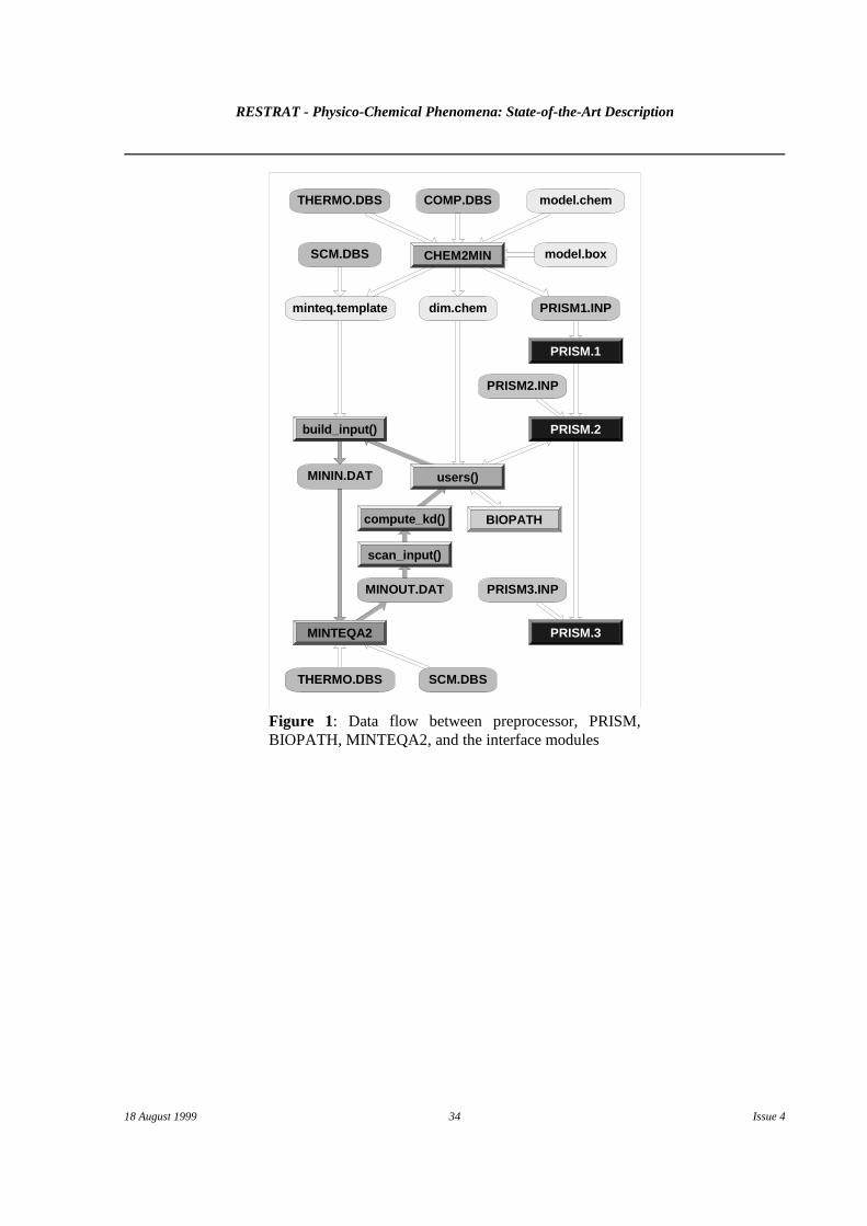
THERMO.DBS
THERMO.DBS COMP.DBS
PRISM3.INP
PRISM2.INP
SCM.DBS
scan_input()
compute_kd()
model.chem
model.box
minteq.template PRISM1.INPdim.chem
MININ.DAT
CHEM2MIN
PRISM.1
PRISM.2build_input()
users()
MINTEQA2
SCM.DBS
MINOUT.DAT
BIOPATH
PRISM.3
RESTRAT - Physico-Chemical Phenomena: State-of-the-Art Description
18 August 1999 34 Issue 4
Figure 1: Data flow between preprocessor, PRISM,BIOPATH, MINTEQA2, and the interface modules
RESTRAT - Physico-Chemical Phenomena: State-of-the-Art Description
18 August 1999 35 Issue 4
10. Conclusions
Reliable risk prognostics for radioactively contaminated sites requires detailed information on the sourceterm. It was demonstrated, that in order to properly describe the evolution of the source term in space andtime an essential part of the information is related to physico-chemical phenomena. An overview over themost important of these phenomena were elaborated, together with their parameter that are necessary formodelling. These parameters can be grouped into three classes:- system-specific parameters for the stationary state;- system-specific parameters for the dynamic evolution;- reaction-specific parameters.
The two classes of system-specific parameters must be determined on the given site. A multidisciplinaryapproach, including radiologists, geologists, hydrologists, chemists, engineers and mathematicians, is notonly required for all later modelling purposes but also to ensure high-quality input data. Especially for thestationary state data, recommendations for sampling techniques and analytical methods were given. Thereaction-specific parameters most often will be extracted from literature, several valuable sources werepointed out, also guidance on the critical evaluation and on the proper usage of such databases is given.This is accompanied by a list of useful methods to be applied in cases were, e.g. thermodynamic, data mustbe determined through own experiments. Most of the discussed physico-chemical phenomena directlycontribute to the chemical speciation of the contaminant of interest. Namely, these are reactions inhomogeneous solution (redox reactions, hydrolysis, complexation, etc), the formation of pure and mixedsolid phases, and reactions on mineral surfaces. The modelling of chemical speciation has to take them allinto account.
This reports describes in detail the state-of-the-art of chemical speciation and migration modelling, givingmany examples of the transition of modelling approaches into software. So far, the complexity of physico-chemical phenomena has not been properly accounted for in risk assessment software. The mainly appliedK concept has several drawbacks but can be substituted by better approaches (unfolding the K into itsd d
main determining processes). This was demonstrated through the development of a new methodology,based on a comprehensive chemical speciation modelling with inclusion of surface complexation reactions( MINTEQA2 [Allison et al., 1991] ) and on the full integration of this part into an existing risk assess-ment software package ( PRISM / BIOPATH [Gardner et al., 1983; Bergström et al., 1982] ). Appropriatesoftware has been developed and tested ( RESTRAT TD7 [Brendler et al., 1999] ). Applications of thenewly developed methodology towards five different test cases are demonstrated in the RESTRAT TD5[Brendler, 1999]. The new approach, and especially the unfolding of the K , makes it possible to performd
more detailed sensitivity analysis, to find the most critical parameters, to reduce the parameter space, andfinally to prepare the way for more reliable models. Thus the objectives of work package WP2.1 are met.
As an outlook the further development of the new approach should be mentioned. This could address, e.g.,the introduction of time-dependence for various chemical parameters coupled to the incorporation ofkinetics to properly describe real geochemical processes with involvement of meta-stable phases. Anotherdirection of further research could be the move to other types of transport models such as the onesdescribed in Section 5.5.2.
RESTRAT - Physico-Chemical Phenomena: State-of-the-Art Description
18 August 1999 36 Issue 4
11. References
Allen PG, Siemering GS, Shuh DK, Bucher JJ, Edelstein NM, Langton CA, Clark SB, Reich T andDenecke MA (1997). Technetium speciation in cement waste forms determined by x-ray absorption finestructure spectroscopy. Radiochimica Acta 76:77
Allison JD, Brown DS and Novo-Gradac KJ (1991). MINTEQA2/PRODEFA2, a geochemical assessmentmodel for environmental systems: Version 3.0 user’s manual. U.S. Environmental Protection Agency,Environmental Research Laboratory, EPA/600/3-91/021
Appelo CAJ and Postma D (1993). Geochemistry, groundwater and pollution. Balkema, Rotterdam
Arnold T, Zorn T, Bernhard G and Nitsche H (1998). Sorption of uranium(VI) onto phyllite. ChemicalGeology 115:129
Ball JW, Nordstrom DK and Zachman DW (1981). U.S. Geological Survey Open File Report 87-50
Beckett R and Hart BT (1993). Use of Field-Flow Fractionation Techniques to Characterize AquaticParticles, Colloids and Macromolecules. In: Buffle J and van Leeuwen HP (eds.). Environmental Particles,IUPAC Series on Environmental Analytical and Physical Chemistry, Volume 2:165. Lewis Publishers,Boca Raton
Bennett DG, Liew SK, Mawbey CS and Read D (1992). CHEMTARD theoretical overview. DOETechnical Report TR-WSA-48
Bergström U and Nordlinder S (1991). Uncertainties related to dose assessments for high level wastedisposal, Nuclear Safety 32:391
Bergström U, Edlund O, Evans S and Röjder B (1982). BIOPATH - A computer code for calculation ofthe turnover of nuclides in the biosphere and the resulting doses to man. Report, Studsvik EnergiteknikAB, Studsvik/NW-82/261, Nyköping
Blum L (1988). Simple method for the computation of thermodynamic properties of electrolytes in themean spherical approximation. Journal of Physical Chemistry. 92:2969
Brendler V (1999). Physico-Chemical Phenomena Governing the Behaviour of Radioactive Substances.Site-specific phenomena. RESTRAT Technical Deliverable TD 5, Report FZ Rossendorf, Institute ofRadiochemistry
Brendler V, Geipel G, Bernhard G and Nitsche H (1996). Complexation in the systemUO /PO /OH (aq): potentiometric and spectroscopic investigations at very low ionic strengths.2 4
2+ 3- -
Radiochimica Acta 74:75
Brendler V, Stiglund Y and Nordlinder S (1999). Risk assessment model for use in site restoration.Software and user instructions. RESTRAT Technical Deliverable TD 7, Report FZ Rossendorf, Instituteof Radiochemistry

RESTRAT - Physico-Chemical Phenomena: State-of-the-Art Description
18 August 1999 37 Issue 4
Broekart JAC, Gücer S and Adams F (1990). Metal Speciation in the Environment. NATO ASI Series G:Ecological Sciences, Vol. 23, Springer, Berlin
Brown PL, Haworth A, Sharland SM and Tweed CJ (1988). HARPHRQ - A geochemical speciationprogram based on PHREEQE. UK Nirex Ltd., Nirex Safety Studies Report NSS/R188
Carnahan CL (1987). Simulation of uranium transport with variable temperature and oxidation potential.The computer program THCC. Mat.Res.Soc.Symp.Proc. 84:713
Connors KA (1990). Chemical Kinetics. The study of reaction rates in solution. VCH, New York
Coudrain-Ribstein A and Jamet P (1988). Le modele geochimique CHIMERE. Principes et noticed'emploi. Centre d'Informatique Geologique Report, Ecole des Mines de Paris, LHM/RD/88/35
Crompton TR (1996). Analysis of Solids in Natural Waters. Springer, Berlin
Davies CW (1962). Ion Association. Butterworths, Washington
Davies RH, Dinsdale AT et al. (1989). MTDATA Handbook. National Physical Laboratory, UK,Documentation for NPL Database for Metallurgical Thermochemistry
Davis JA, James RO and Leckie JO (1978). Surface Ionization and Complexation at the Oxide/WaterInterface 1. Computation of Electrical Double Layer Properties in Simple Electrolytes. Journal of Colloidand Interface Science 63:481
Davis JA and Kent DB (1990). Surface complexation modelling in aqueous geochemistry. In: HochellaMF and White AF (eds.). Mineral-water interface geochemistry. Reviews in Mineralogy 23:177
Davis JA and Leckie JO (1978). Surface Ionization and Complexation at the Oxide/Water Interface II.Surface properties of Amorphous Iron Oxyhydroxide and Adsorption of Metal Ions. Journal of Colloid andInterface Science 67:90
Davis JA and Leckie JO (1980). Surface Ionization and Complexation at the Oxide/Water Interface 3.Adsorption of Anions. Journal of Colloid and Interface Science 74:32
Denecke MA, Reich T, Pompe S, Bubner M, Heise KH, Nitsche H, Allen PG, Bucher JJ, Edelstein NM,Shuh DK (1997). Differentiating between Monodentate and Bidentate Carboxylate Ligands Coordinatedto Uranyl Ions Using EXAFS. J. Physics. IV France 7(C2):637
De Nobili M, Gjessing E, and Sequi P (1989). Sizes and shapes of humic substances by gel chromatogra-phy. In: Hayes MHB, MacCarthy P, Malcolm RB, and Swift RS (eds.). Humic substances II - In search ofstructure, Wiley Interscience, Chichester
Deutsch WJ (1997). Groundwater Geochemistry. Fundamentals and Application to Contamination. LewisPublishers, Boca Raton
Dzombak DA and Morel FMM (1990). Surface complexation modelling. Hydrous ferric oxide. Wiley,New York

RESTRAT - Physico-Chemical Phenomena: State-of-the-Art Description
18 August 1999 38 Issue 4
Eriksson G (1979). An algorithm for the computation of aqueous multicomponent, multiphase equilibria.Analytica Chimica Acta 112:375
Eriksson G and Hack K (1990). ChemSage - a computer program for the calculation of complex chemicalequilibria. Metallurgical Transactions B 21:1013
Fränzle O (1993). Contaminants in terrestrial environments. Springer, Berlin
Gans P (1992). Data Fitting in the Chemical Sciences by the Method of Least Squares. Wiley, Chichester
Gardner RH, Röjder B and Bergström U (1983). PRISM - A systematic method for determining the effectof parameter uncertainties on model predictions. Report, Studsvik Energiteknik AB, Studsvik/NW-83/555,Nyköping
Geipel G, Brachmann A, Brendler V, Bernhard G and Nitsche H (1997a). Uranium(VI) sulfatecomplexation studied by time-resolved laser-induced fluorescence spectroscopy (TRLFS). RadiochimicaActa 75:199
Geipel G, Reich T, Brendler V, Bernhard G and Nitsche H (1997b). Laser and X-Ray SpectroscopicStudies of Uranium-Calcite Interface Phenomena. Journal of Nuclear Materials 248:408
Goldberg S (1991). Sensitivity of Surface Complexation Modelling to the Surface Site Density Parameter.Journal of Colloid and Interface Science 145:1
Grenthe I, Plyasunov AV and Spahiu K (1997). Estimations of medium effects on thermodynamic data.In: Grenthe I and Puigdomenech I (eds.). Modelling in Aquatic Chemistry, 325, OECD-NEA, Paris
Hamer K and Sieger R (1994). Anwendung des Modells COTAM zur Simulation von Stofftransport undgeochemischen Reaktionen, Verlag Ernst & Sohn
Haworth A, Sharland SM, Tasker PW and Tweed CJ (1988). Extensions to the coupled chemical equilibriaand migration code CHEQMATE. UK Nirex Ltd., Nirex Safety Studies Report NSS/R115
Hayes KF, Redden G, Ela W and Leckie JO (1991). Surface Complexation Models: An evaluation ofmodel parameter estimation using FITEQL and oxide mineral titration data. Journal of Colloid andInterface Science 142:448
Heames TJ, Williams DA, Bixler NE, Grimley AJ, Wheatley CJ, Johns NA, Domagala P, Dickson LW,Alexander CA, Osborn-Lee I, Zawadzki S, Rest J, Mason A, and Lee RY (1992). VICTORIA : AMechanistic Model of Radionuclide Behavior in the Reactor Coolant System Under Severe AccidentConditions. Sandia National Laboratory, Report NUREG/CR-5545, SAND 90-0756, R3, R4, Rev1; Albu-querque
Horne RA (1971). Water and aqueous solutions. Structure, thermodynamics, and transport processes.Wiley-Interscience, New York
Ingri N, Andersson I, Pettersson L, Yagasaki A, Andersson L and Holmström K (1996). LAKE - Aprogram system for equilibrium analytical treatment of multimethod data, especially combined potentio-metric and nuclear magnetic resonance data. Acta Chemica Scandinavica 50:717

RESTRAT - Physico-Chemical Phenomena: State-of-the-Art Description
18 August 1999 39 Issue 4
Ivanovich M, Swanton SW, Russell PJ, Read D, Thomas J, Tipping E and Hurley MA (1993). Develop-ment and testing of a coupled-process model incorporating colloidal phase: A study of thorium transportin the presence of silica colloids. UK DoE Report, DOE/HMIP/RR/94/036
Jeffery PG and Hutchison D (1986). Chemical Methods of Rock Analysis. Pergamon Series in AnalyticalChemistry, Vol. 4. Pergamon Press, Oxford
Jenne EA (1979). Chemical modelling in aqueous systems. ACS symposium series 93, ACS, Washington
Kienzler B (1995). A Coupled Migration/Speciation Code - Demonstrated by Modelling the Migration ofAmericium in a Column. Proceedings International Conference on Mathematics & Computations, ReactorPhysics & Environmental Analysis, Portland, U.S.A.
Klein T and Nießner R (1998). Characterization of Heavy Metal Containing Seepage Water Colloids byFlow FFF, Ultrafiltration, ELISA and AAS. Microchimica Acta 129:47
Leggett DJ (1985). SQUAD: Stability quotients from absorbance data. In: Leggett, DJ (ed.). Computa-tional methods for the determination of formation constants, 159-173, Plenum Press, New York
Leung VW-H, Darvell BW and Chan AP-C (1988). A rapid algorithm for solution of the equations ofmultiple equilibrium systems - RAMESES. Talanta 35:713
Lichtner PC, Steefel CI and Oelkers EH (1996). Reactive Transport in porous media. Reviews in Mineral-ogy 34
Lim TK (1987). A new method for calculating activity coefficients of mixed electrolytes. Journal ofSolution Chemistry 16:11
Liu CW and Narasimhan TN (1989). Redox-Controlled Multiple-Species Reactive Chemical Transport,1. Model Development. Water Resources Research, 25:869
Liu CW and Narasimhan TN (1989). Redox-Controlled Multiple-Species Reactive Chemical Transport,2. Verification and Application. Water Resources Research, 25:882
Manahan S (1994). Environmental Chemistry. 6th ed., Lewis Publishers (CRC Press), Boca Raton
Martell AE and Motekaitis RJ (1992). Determination and use of stability constants. 2nd ed., VCH, NewYork
Mason P, Lemire R, Vuorinen U, Madic C, Kienzler B, Qaim S, Ogawa T, Park KK, Konings R, GrentheI and Fuger J (1996). Survey of Thermodynamic and Kinetic Databases. NEA/NSC/DOC(96)27
Melchior DC and Bassett RL (1990). Chemical modelling of aqueous systems II. ACS symposium series416, ACS, Washington
Meloun M, Havel J and Högfeldt E (1988). Computation of solution equilibria: a guide to methods inpotentiometry, extraction, and spectrophotometry. Horwood, Chichester

RESTRAT - Physico-Chemical Phenomena: State-of-the-Art Description
18 August 1999 40 Issue 4
Moll H, Matz W, Schuster G, Brendler E, Bernhard G and Nitsche H (1995). Synthesis and Characteriza-tion of Uranyl-Orthosilicate (UO )SiO ·2H O. Journal of Nuclear Materials 227:402 4 2
Moll H, Geipel G, Matz W, Bernhard G and Nitsche H (1996). Solubility and speciation of(UO ) SiO ·2H O in aqueous systems. Radiochimica Acta 74:32 2 4 2
Moll H, Geipel G, Brendler V, Bernhard G and Nitsche H (1998). Interaction of uranium(VI) with silicicacid in aqueous solutions studied by time-resolved laser-induced fluorescence spectroscopy (TRLFS).Journal of Alloys and Compounds 271-273:765
Moreno RA, Barrdahl R, Bergström U and Nordlinder S (1995). Comparison of BIOPATH andMARCEN. Report, Swedish Radiation Protection Institute, SSI-Rapport 95-23, Stockholm
Nitzsche O (1997). TReAC-Modell zur Beschreibung des reaktiven Stofftransports im Grundwasser. Wiss.Mitteilungen Inst. Geologie 1/1997, TU Bergakademie Freiberg, Freiberg
Noorishad J, Carnahan CL and Benson LV (1987). Development of the non-equilibrium reactive chemicaltransport code CHEMTRNS. Lawrence Berkeley Laboratory, University of California, Report LBL-22361
Nordlinder S, Aggeryd I, Bergström U and Sundblad B (1995). Environmental risk assessment for theSillamäe waste repository. Proceedings International Symposium on Environmental Impact of RadioactiveReleases, IAEA, Vienna
Nordlinder S, Bergström U, Hammar J and Notter M (1993). Modelling turnover of Cs-137 in twosubarctic salmonid ecosystems. Nordic Journal of Freshwater Research 68:21
Östhols E (1994). The C-Letagrop program system. Version 1.4. Royal Institute of Technology Report,TRITA-OOK-2051, Stockholm
Östhols E (1994). The C-Haltafall program system for equilibrium speciation calculations. Version 1.7.Royal Institute of Technology Report, TRITA-OOK-2062, Stockholm
Papelis C, Hayes KF and Leckie LO (1988). HYDRAQL: A program for the computation of chemicalequilibrium composition of aqueous batch systems including surface-complexation modelling of ionadsorption at the oxide/solution interface. Department of Civil Engineering, Stanford University, TechnicalReport 306, Stanford
Parkhurst DL, Thorstenson DC and Plummer LN (1980). PHREEQE - A computer program for geochemi-cal calculations. U.S. Geological Survey Water-Resources Investigations, Report 80-96
Parkhurst DL (1995). User's guide to PHREEQC - A computer program for speciation, reaction-path,advective-transport, and inverse geochemical calculations. U.S. Geological Survey Water-ResourcesInvestigations, Report 95-4227
Pecora R (ed.) (1985). Dynamic Light Scattering. Plenum Press, New York and London
Perkins EH, Kharaka YK, Gunter WD and DeBraal JD (1990). Geochemical modelling of water-rockinteractions using SOLMINEQ.88. In: Melchior DC and Bassett RL (eds). Chemical modelling of aqueoussystems II, ACS symposium series 416:117, ACS, Washington

RESTRAT - Physico-Chemical Phenomena: State-of-the-Art Description
18 August 1999 41 Issue 4
Perry DL (1990). Instrumental surface analysis of geologic materials. VCH, Weinheim
Phillies GDJ (1990). Quasielastic Light Scattering. Analytical Chemistry 62:1049A
Pitzer KS (1973). Thermodynamics of electrolytes. I. Theoretical basis and general equations. Journal ofPhysical Chemistry. 77:268
Pitzer KS (1991). Activity coefficients in electrolyte solutions. 2nd ed., CRC Press, Boca Raton
Plummer LN, Parkhurst DL, Fleming GW and Dunkle SA (1988). A computer program incorporatingPitzer’s equations for calculation of geochemical reactions in brines. U.S. Geological Survey Wa-ter-Resources Investigations, Report 88-4153
Puigdomenech I and Bergström U (1994). Calculated distribution of radionuclides in soils and sediments.SKB Technical Report 94-32, Stockholm
Read D (1994). Chemval-2 project. Report on stage 1: status of six technical areas. CEC Nuclear Scienceand Technology, Report EUR 15161, Luxembourg
Reich T, Moll H, Denecke MA, Geipel G, Bernhard G, Nitsche H, Allen PG, Bucher JJ, Kaltsoyannis N,Edelstein NM and Shuh DK (1996). Characterization of hydrous uranyl silicate by EXAFS. RadiochimicaActa 74:219
Scatchard G (1968). Excess free energy and related properties of solutions containing electrolytes. Journalof the American Chemical Society 90:3124
Schecher WD and McAvoy DC (1994). MINEQL : A Chemical Equilibrium Program for personal+
Computers. User's Manual Version 3.0. Environmental Research Software, Hallowell, ME 04347, U.S.A.
Schimpf ME and Wahlund KG (1997). Asymmetrical Flow Field-Flow Fractionation as a Method to Studythe Behavior of Humic Acids in Solution. J. Microcolumn. Separations 9:535
Schmalzried H (1995). Chemical Kinetics of Solids. VCH, Weinheim
Schnoor JL (1996). Environmental Modeling. Fate and Transport of Pollutants in Water, Air, and Soil.Wiley-Interscience, New York
Schurtenberger P and Newman ME (1993). Characterization of Biological and Environmental ParticlesUsing Static and Dynamic Light Scattering. In: Buffle J and van Leeuwen HP (eds.). EnvironmentalParticles. IUPAC Series on Environmental Analytical and Physical Chemistry, Volume 2:37-116. LewisPublishers, Boca Raton
Simunek J and Suarez DL (1993). UNSATCHEM-2D Code for Simulating Two-Dimensional VariablySaturated Water Flow, Heat Transport, Carbon Dioxide Production and Transport, and MulticomponentSolute Transport with Major Ion Equilibrium and Kinetic Chemistry, Version 1.1 Manual. ResearchReport No. 128, U.S. Department of Agriculture, Riverside
Sposito G (1983). On the Surface Complexation Model of the Oxide-Aqueous Solution Interface. Journalof Colloid and Interface Science 91:329

RESTRAT - Physico-Chemical Phenomena: State-of-the-Art Description
18 August 1999 42 Issue 4
Sposito G (1989). Surface Reactions in Natural Aqueous Colloidal Systems. Chimia 43:169
Sposito G and Mattigod SV (1980). GEOCHEM: A computer program for the calculation of chemicalequilibria in soil solutions and other natural water systems. Department of Soil Science, Report, KeerneyFoundation of Soil Science, University of California, Berkeley
Steefel CI and Yabusaki SB (1995). OS3D/GIMRT - Software for modelling multicomponent-multidimen-sional reactive transport. User manual & programmer’s guide version 1.0. Battelle Memorial Institute
Stiglund Y and Nordlinder S (1999). Dose Assessment Model for use in site restoration. General method-ology and site-specific aspects. RESTRAT Technical Deliverable TD 6, Report Studsvik Eco & SafetyAB, Nyköping
Stumm W (1992). Chemistry of the solid-water interface. Wiley, New York
Stumm W and Morgan JJ (1996). Aquatic chemistry: chemical equilibria and rates in natural waters.3rd ed., Wiley, New York
Swift RS (1985). Fractionation of soil humic substances. In: Aiken GR (ed.). Humic substances in soil,sediment, and water. Wiley Interscience, New York
Teterin YA, Nefedov VI, Ivanov KE, Baev AS, Geipel G, Reich T and Nitsche H (1996). X-ray photoelec-tron spectroscopy investigation of UO (ClO ) with calcite and diabase minerals. Zhurnal2 4 2
Neorganisheskoyi Khimii 41:1884
Truesdell AH and Jones BF (1973). WATEQ, a computer program for calculating chemical equilibria ofnatural waters. U.S. Geological Survey, National Technical Information Service, PB-220 464
Ure AM and Davidson CM (1995). Chemical Speciation in the Environment. Blackie Academic &Professional, London
Vacca A and Sabatini A (1985). MINIQUAD and MIQUV: Two approaches for the computation offormation constants from potentiometric data. In: Leggett, DJ (ed.). Computational methods for thedetermination of formation constants, 99. Plenum Press, New York
Van der Lee J, Ledoux E, De Marsily G, Vinsot A, Van de Weerd H, Leijnse A, Harmand B, Rodier E,Sardin M, Dodds J and Hernández Benítez A (1997). Development of a model for radionuclide transportby colloids in the geosphere. CEC Nuclear Science and Technology, Report EUR 17480, Luxembourg
Walter AL, Frind EO, Blowes DW, Ptacek CJ and Molson JW (1994). Modeling of multicomponentreactive transport in groundwater. I. Model development and evaluation. Water Resources Research30:3137
Westall JC, Zachary JL and Morel FMM (1976). MINEQL, a computer program for the calculation ofchemical equilibrium composition of aqueous systems. Technical Note 18, Department of ChemicalEngineering, MIT, Cambridge, MA
Westall JC (1982). FITEQL - A computer program for determination of chemical equilibrium constantsfrom experimental data. Department of Chemistry, Oregon State University, Report 82-02, Corvallis
RESTRAT - Physico-Chemical Phenomena: State-of-the-Art Description
18 August 1999 43 Issue 4
Wolery TJ (1992). EQ3/6, A software package for the geochemical modelling of aqueous systems.UCRL-MA-110662 Part I, Lawrence Livermore National Laboratory
Yeh GT and Tripathi VS (1990). HYDROGEOCHEM: a coupled model of hydrologic transport andgeochemical equilibria in reactive multi-component systems. Oak Ridge National Laboratory, ReportORNL-6372
Zheng C and Wang PP (1998), MT3DMS: Documentation and User’s Guide, Report to the U.S. ArmyCorps of Engineers Waterways Experiment Station. University of Alabama, Tuscaloosa, Alabama

RESTRAT - Physico-Chemical Phenomena: State-of-the-Art Description
18 August 1999 44 Issue 4
12. Acknowledgment
There are many people who contributed to this report. First I would like to mention my colleague ThuroArnold, who helped me to understand surface complexation, and the behaviour of minerals in naturalenvironments. Yvonne Stiglund (now at VBB in Nyköping), Sture Nordlinder, and Ignasi Puigdomenech(now at KTH in Stockholm) from Studsvik Eco & Safety AB in Nyköping / Sweden helped me tounderstand and work with the PRISM / BIOPATH package. The project coordinator, Theo Zeevaert fromSCK-CEN in Mol / Belgium improved the report with many remarks, also Duncan Jackson, StewartWragg (now at BNFL), and Andrew Bousher from Westlakes Scientific Consultants / Great Britain.
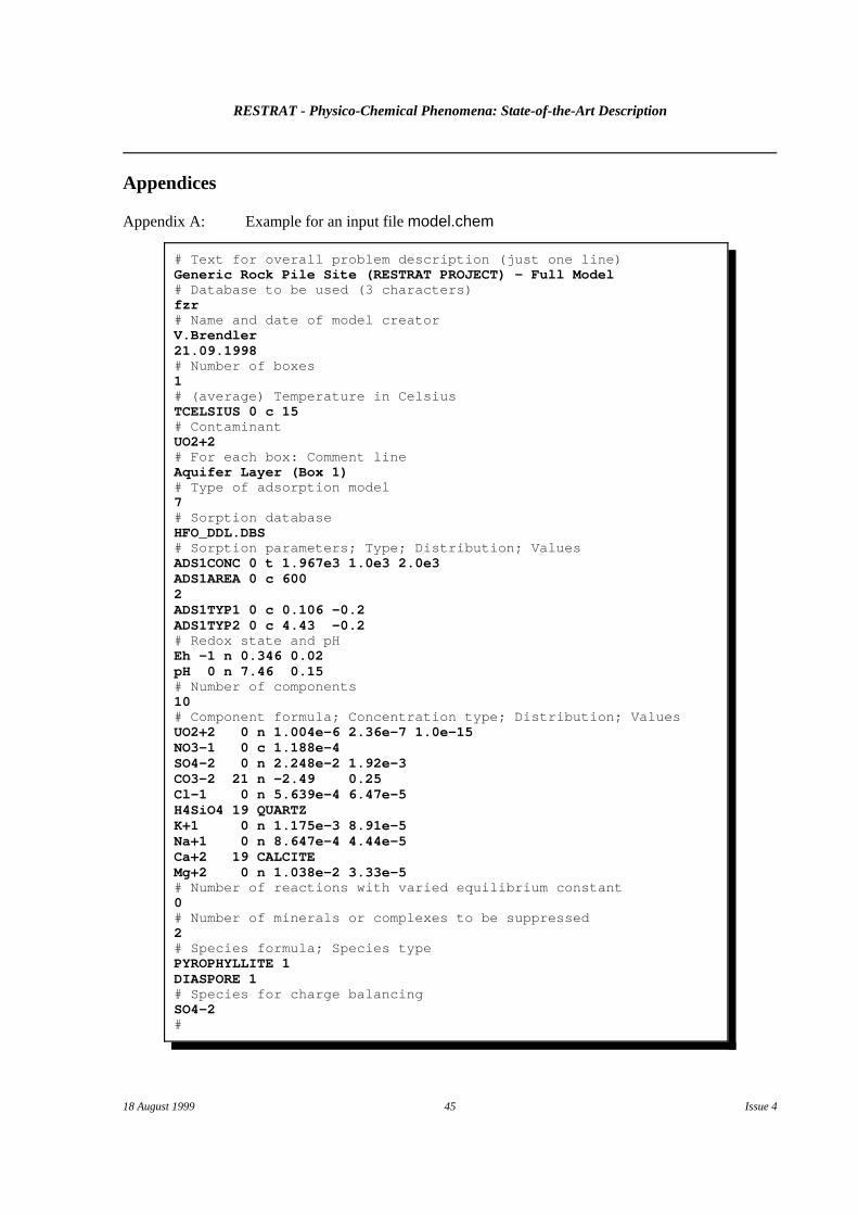
RESTRAT - Physico-Chemical Phenomena: State-of-the-Art Description
18 August 1999 45 Issue 4
# Text for overall problem description (just one line)Generic Rock Pile Site (RESTRAT PROJECT) - Full Model# Database to be used (3 characters)fzr# Name and date of model creatorV.Brendler21.09.1998# Number of boxes1# (average) Temperature in CelsiusTCELSIUS 0 c 15# ContaminantUO2+2# For each box: Comment lineAquifer Layer (Box 1)# Type of adsorption model7# Sorption databaseHFO_DDL.DBS# Sorption parameters; Type; Distribution; ValuesADS1CONC 0 t 1.967e3 1.0e3 2.0e3ADS1AREA 0 c 6002ADS1TYP1 0 c 0.106 -0.2ADS1TYP2 0 c 4.43 -0.2# Redox state and pHEh -1 n 0.346 0.02pH 0 n 7.46 0.15# Number of components10# Component formula; Concentration type; Distribution; ValuesUO2+2 0 n 1.004e-6 2.36e-7 1.0e-15NO3-1 0 c 1.188e-4SO4-2 0 n 2.248e-2 1.92e-3CO3-2 21 n -2.49 0.25Cl-1 0 n 5.639e-4 6.47e-5H4SiO4 19 QUARTZK+1 0 n 1.175e-3 8.91e-5Na+1 0 n 8.647e-4 4.44e-5Ca+2 19 CALCITEMg+2 0 n 1.038e-2 3.33e-5# Number of reactions with varied equilibrium constant0# Number of minerals or complexes to be suppressed2# Species formula; Species typePYROPHYLLITE 1DIASPORE 1# Species for charge balancingSO4-2#
Appendices
Appendix A: Example for an input file model.chem
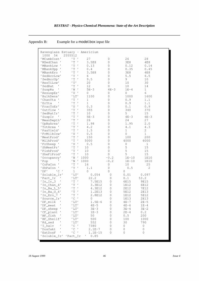
RESTRAT - Physico-Chemical Phenomena: State-of-the-Art Description
18 August 1999 46 Issue 4
Ravenglass Estuary - Americium 1000 54 2555512’MCumbCost’ ’T ’ 27 0 26 28’MSedChan ’ ’T ’ 3.5E8 0 3E8 4E8’MBankLow ’ ’T ’ 0.13 0 0.12 0.14’MBankUpp ’ ’T ’ 0.4 0 0.35 0.45’MBankEro ’ ’T ’ 3.5E8 0 3E8 4E8’SedAccLow’ ’T ’ 6 0 5.5 6.5’SedAccUp’ ’T ’ 9.5 0 9 10’ResTiLow’ ’T’ 20 0 10 30’SedRat ’ ’T ’ 12 0 10 14’SuspRa ’ ’N ’ 5E-3 4E-3 1E-4 1’ResuspEr’ ’U ’ 0 0 0 6’BulkDens’ ’LT’ 1100 0 1000 1600’ChanYta ’ ’T ’ 1 0 0.9 1.1’ErYta ’ ’T ’ 1 0 0.9 1.1’FracToEr’ ’U ’ 0.3 0 0.1 0.9’Outflow ’ ’T ’ 355 0 340 370’SedRatIr’ ’T ’ 10 0 5 15’SuspIr ’ ’T ’ 5E-3 0 4E-3 6E-3’MeanDepth’ ’T ’ 26 0 24 27’UpBaArea’ ’T ’ 1.98 0 1.95 2.0’TotArea ’ ’T ’ 4.2 0 4.1 4.3’PasYield’ ’T ’ 1.5 0 1 2’FrMilkCow’ ’U ’ 0.5 0 0 1’MeatProd’ ’T ’ 150 0 100 200’MilkProd’ ’T ’ 5000 0 4000 6000’FrSheep ’ ’U ’ 0.5 0 0 1’ShMeetPr’ ’T ’ 10 0 5 15’FishProd’ ’T ’ 10 0 5 15’SheFiProd’ ’T ’ 10 0 5 15’Occupancy’ ’N ’ 1000 -0.2 1E-10 1E10’Pop ’ ’N ’ 1000 -0.2 1E-10 1E10’CoPaCon ’ ’T ’ 16 0 10 25’ShPaCon ’ ’T ’ 1.1 0 0.5 2’DF’ ’C ’ 1 0 0 0’Soluble_Ir’ ’LT’ 0.054 0 0.01 0.097’Part_Ir ’ ’LT’ 22.2 0 0.1 53.2’In_Ir_3 ’ ’T ’ 7.5E15 0 6E15 9E15’In_Chan_4’ ’T ’ 3.3E12 0 1E12 6E12’In_Ba_L_5’ ’T ’ 4.3E12 0 2E12 7E12’In_Ba_U_6’ ’T ’ 1.2E13 0 5E12 2E13’In_Ero_7 ’ ’T ’ 2.8E12 0 1E12 5E12’Source_Ir’ ’C ’ 0 0 1E13 2E13’DF_milk ’ ’LT’ 1.5E-6 0 4E-7 2E-5’DF_meat ’ ’LT’ 4E-5 0 4E-6 1E-4’DF_sheep ’ ’LT’ 3E-3 0 3E-4 3E-2’CF_plant ’ ’LT’ 1E-3 0 2E-4 0.2’BF_fish ’ ’LT’ 50 0 0.5 200’BF_Shellf’ ’LT’ 500 0 100 1000’Kd_sed ’ ’LT’ 552 0 30 790’T_halv ’ ’C ’ 7380 0 0 0’Dosfakt ’ ’C ’ 2.1E-7 0 0 0’ExtDosF ’ ’C ’ 1.1E-15 0 0 0’Soluble_Ir’ ’Part_Ir ’ 0.85
Appendix B: Example for a model.box input file

RESTRAT - Physico-Chemical Phenomena: State-of-the-Art Description
18 August 1999 47 Issue 4
Generic Rock Pile Site (RESTRAT PROJECT) - Full ModelCreated at: 21.09.1998Created by: V.BrendlerBox 1: Aquifer Layer (Box 1)#@#PARA001## MOLAL 0.0000 0 1 1 2 0 0 0 1 3 0 0 04 1 7#@#PARA002## #@#PARA003## #@#PARA006## #@#PARA007## 81 1 0.0 0.00 /E-1 330 0.0 0.00 /H+1 893 #@#PARA010## -15.00 n /UO2+2 492 #@#PARA011## 0.00 /NO3-1 732 #@#PARA012## 0.00 /SO4-2 140 0.0 0.00 /CO3-2 180 #@#PARA014## 0.00 /Cl-1 770 0.0 0.00 /H4SiO4 410 #@#PARA015## 0.00 /K+1 500 #@#PARA016## 0.00 /Na+1 150 0.0 0.00 /Ca+2 460 #@#PARA017## 0.00 /Mg+2 811 #@#PARA004## 0.00 /ADS1TYP1 812 #@#PARA005## 0.00 /ADS1TYP2 813 0.0 0.00 /ADS1PSIo
3 5 330 #@#PARA009## 0.00 /H+13301403 #@#PARA013## 0.00 /CO2 (g) 1 #@#PARA008## 0.00 /E-12077002 4.0060 0.00 /QUARTZ5015001 8.4750 0.00 /CALCITE 6 38603002 0.0 0.00 /PYROPHYLLITE2003002 0.0 0.00 /DIASPORE 813 0.0 0.00 /ADS1PSIo
Appendix C: Example for a MINTEQA2 input template
This example was generated based on the chemical input file shown in Appendix A, but it does not showthe sorption database that will also be appended automatically on the MINTEQA2 input file template.