Physically Guided Liquid Surface Modeling from Videos

Huamin Wang∗ Miao Liao† Qing Zhang† Ruigang Yang† Greg Turk∗

Georgia Institute of Technology∗ University of Kentucky†

Figure 1: A synthetic rendering of a 3D model reconstructed from video of a fountain. These are three static views of the same time instant.

Abstract

We present an image-based reconstruction framework to model realwater scenes captured by stereoscopic video. In contrast to manyimage-based modeling techniques that rely on user interaction toobtain high-quality 3D models, we instead apply automatically cal-culated physically-based constraints to refine the initial model. Thecombination of image-based reconstruction with physically-basedsimulation allows us to model complex and dynamic objects suchas fluid. Using a depth map sequence as initial conditions, we usea physically based approach that automatically fills in missing re-gions, removes outliers, and refines the geometric shape so that thefinal 3D model is consistent to both the input video data and thelaws of physics. Physically-guided modeling also makes interpola-tion or extrapolation in the space-time domain possible, and evenallows the fusion of depth maps that were taken at different timesor viewpoints. We demonstrated the effectiveness of our frameworkwith a number of real scenes, all captured using only a single pairof cameras.

CR Categories: I.3.5 [COMPUTER GRAPHICS]: Computa-tional Geometry and Object Modeling—Physically based model-ing; I.3.8 [COMPUTER GRAPHICS]: Three- Dimensional Graph-ics and Realism—Animation

Keywords: image-based reconstruction, space-time model com-pletion, physically-based fluid simulation

1 Introduction

∗e-mail: {whmin, turk}@cc.gatech.edu†e-mail: {mliao3, qzhan7, ryang}@cs.uky.edu

In recent years, modeling complex real world objects and scenesusing cameras has been an active research topic in both graphicsand vision. Exemplary work in this broad topic includes recon-structing flower models [Quan et al. 2006], tree models [Tan et al.2007], hairs [Wei et al. 2005], urban buildings [Sinha et al. 2008;Xiao et al. 2008], human motion [Zitnick et al. 2004a; de Aguiaret al. 2008], and cloth [White et al. 2007; Bradley et al. 2008]. Thetypical approach is to use one or more cameras to capture differ-ent views, from which the 3D shape information of the scene canbe estimated by matching feature points. User interaction is oftenrequired to refine the initial 3D shape to create high-quality mod-els. Missing from the list of objects that have been successfully re-constructed from video is water. Water’s complex shape, frequentocclusions, and generally non-Lambertian appearance cause eventhe best matching methods to yield poor depth maps. Its dynamicnature and complex topological changes over time make human re-finement too tedious for most applications.

In computer graphics, a common technique to produce water ani-mation is physically-based fluid simulation, which is based on sim-ulating fluid dynamics from the initial state of a fluid scene. Whilerealistic water animation can be generated by various numericalsimulation approaches, these approaches can suffer from numer-ical errors that accumulate over time, including volume loss andloss of surface details. The computational cost is another issue inphysically based fluid simulation, since the governing partial differ-ential equations are expensive to solve and the time steps need tobe sufficiently small to maintain stability and accuracy.

In this paper we present the idea of combining physically-basedsimulation with image-based reconstruction to model dynamic wa-ter from video. That is, we adapt physically-based methods as acorrection tool to refine the water surface that is initially gener-ated from matching feature points. In order to enforce temporalcoherence, we develop a 3D flow estimation method to approxi-mate the velocity flow between two reconstructed shapes in neigh-boring frames. The surface optimization method then removes re-dundant errors, applies physically based constraints such as volumepreservation and smoothness, and completes the shape sequence byfilling in missing fluid regions. In this way, the final dynamic wa-ter model matches the fidelity of the real world and the results arephysically sound, even though fluid dynamics may not be strictlyenforced in certain cases. Since fluid dynamics is only used as a

constraint rather than the target function to derive the entire surfacesequence, this process is efficient and should be easy to accelerateusing graphics hardware.

Incorporating the physical properties of fluid provides strong con-straints on the possible water surface shape. This means the qualityand coverage requirement for the initial 3D shape is significantly re-duced. This allows us to generate plausible 3D water surface mod-els even when observed by just one stereo camera, that is, whenmore than 50% of the surface is occluded. A single-depth-view so-lution is much easier to set up and use than the typical requirementof a surrounding array of cameras.

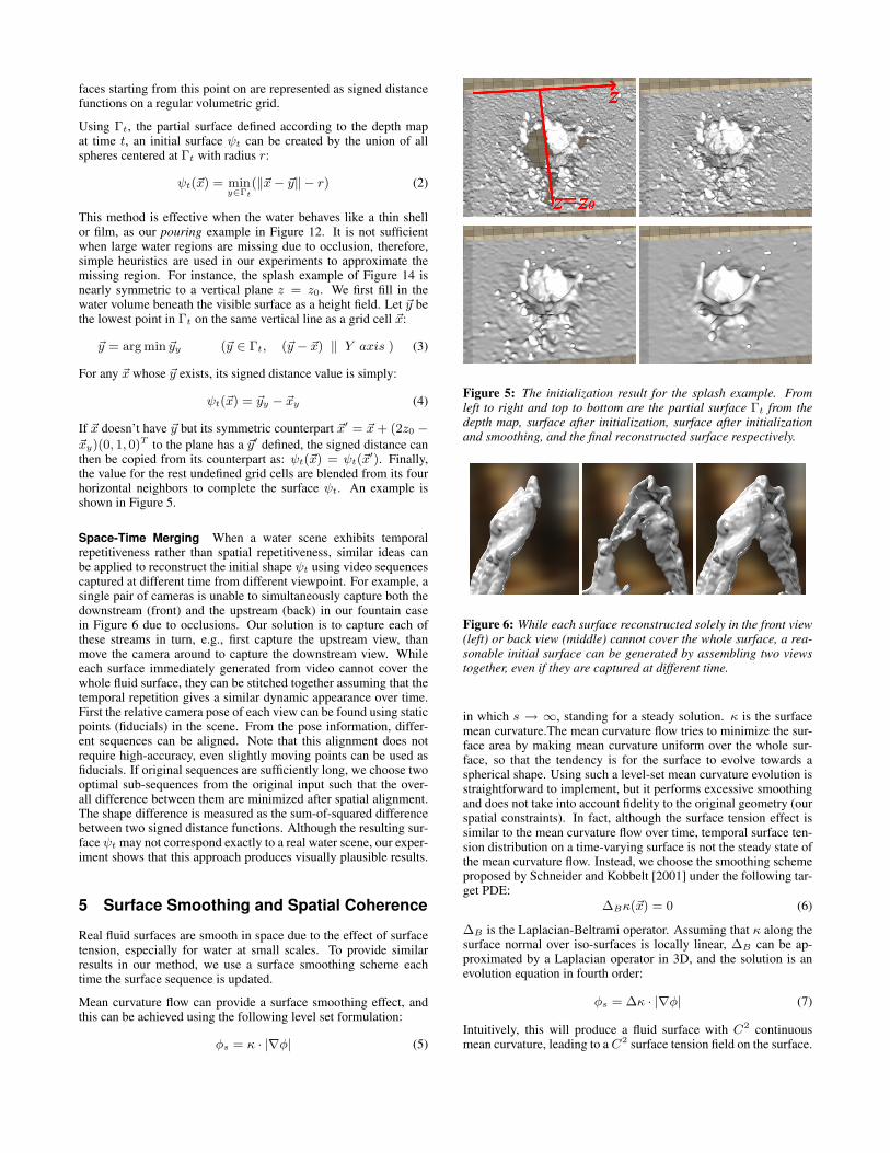
To help with spatial feature matching, we add white paint to the wa-ter to avoid refraction, and we use a light projector to place a fixedrandom texture pattern onto the moving fluid surfaces. The equip-ment used for our capturing system is shown in Figure 3. Note thatour surface optimization scheme is not tied to any particular depthacquisition method, nor does it require appearance-based featuretracking over time, and this makes the use of active range sensingmethods possible. Our choice of using a stereo camera in this sys-tem is due to two considerations. First, since this technique can bepotentially used with any capturing device, it is interesting to test itsperformance in a tough case when less surface information is pro-vided. Second, one part of our ultimate goal of this line of researchis to reconstruct large, outdoor fluid phenomena, in which case ahand-held stereo camera is much more practical than a surroundingmulti-camera system.

We view this new approach for creating fluid models as an alter-native to creating fluid animation through direct simulation. Aswith other camera-based data capture methods, our approach hasthe benefit of capturing the nuances and details of fluids that maybe difficult to achieve using simulation alone. With an explicit3D model, the captured water can be re-rendered seamlessly withother graphics models. Though not demonstrated in this paper, ourframework should allow artists to design and modify a coarse initialshape in order to create stylized animations. Therefore we believethat our method may have applications in feature-film special ef-fects and in video game content creation.

2 Related Work

In graphics, Hawkins et al. [2005] demonstrated how to reconstructsmoke animation using a specialized capture system that includeda laser and a high-speed camera. Morris and Kutulaskos [2007]and Hullin et al. [2008] successfully reconstructed static transpar-ent objects such as a vase or a glass by tracing light transport understructured scanning. A time-varying height-field surface can alsobe reconstructed by searching refractive disparity as proposed byMorris and Kutulakos [2005] when the light is refracted only once.Water thickness can be measured when water is dyed with fluores-cent chemical as shown by Ihrke et al. [2005], in which case the liq-uid surface is calculated as a minimum solution of a photo consis-tency based error measure using the Euler-Lagrangian formulation.Atcheson et al. [2008] used Schlieren tomography to capture fluidswith time-varying refraction index values, such as heated smoke. Ingeneral, these techniques require specific capture devices for cer-tain fluid effects and they consider the fluid shape in each frameindependently as a static reconstruction problem.

Bhat et al. [2004] studied how to synthesize new fluid videos bytracing textured 2D particles over existing video sequences accord-ing to temporal continuity. This is an image editing approach,and no 3D model is created. Given surrounding reliable scanneddata without redundant errors, Sharf et al. [2008] successfully usedincompressible flow to complete shape animations with spatial-temporal coherence, assuming that the surface moves less than one

grid cell in each time step. Although fluid animation also satisfiesincompressibility with spatial-temporal coherence, the problem weaddress in this paper is more challenging since the input is capturedfrom a single stereo camera, so our initial water surface containsoutliers and substantially more missing parts than from a surround-ing setup. Furthermore the water surface can move significantlymore than one grid cell due to the capture rate and grid resolution.

Foster and Metaxas [1996] studied how to generate fluid animationas an application of computational fluid dynamics. Shortly afterthis, the stable fluid method introduced by Stam [1999] used thesemi-Lagrangian method to handle fluid velocity advection. In aseries of papers, Enright, Fedkiw and Foster [2001; 2002] used thelevel set method and particles to evolve liquid surfaces for morecomplex liquid motions. Besides volumetric representation, wateranimation can also be simulated using particle systems or tetrahe-dral meshes. When using fluid dynamics, numerical errors includ-ing volume loss and detail loss can be a problem in physically basedfluid simulation. Another problem in this area is how to reach styl-ized fluid shapes at specified time instants. McNamara et al. [2004]and Fattal and Lischinski [2004] studied how to constrain fluid sim-ulation by creating artificial control forces. In our problem, we con-sider instead how to improve reconstructed models by physically-based constraints.

Researchers in other domains have used various techniques to cap-ture the behavior of fluids. The fluid imaging community regularlymakes use of the Particle Imaging Velocimetry (PIV) method tocapture flow fields from the real world by tracking macroscopic par-ticles mixed in the fluid. This method creates fluid velocity valuesin the interior of bodies of water, but the approach cannot be usedto reconstruct the geometry of the water’s surface due to the diffi-culty in maintaining the distribution of those particles in the fluid.More details of the PIV method can be found in [Grant 1997].

To obtain a complete space+time model from dynamic scenes, acamera array system is usually deployed to capture objects fromdifferent views (e.g., [Kanade et al. 1999; Simon et al. 2000; Zit-nick et al. 2004b]). Recently using a sparse camera array becomesan active research topic (e.g., [Wand et al. 2007; Mitra et al. 2007;Sharf et al. 2008]. We push this trend to the limit by using onlyone pair of cameras with a narrow baseline. We show that by in-corporating physically-based constraints, the amount of input dataneeded for complete 4D modeling can be dramatically reduced.

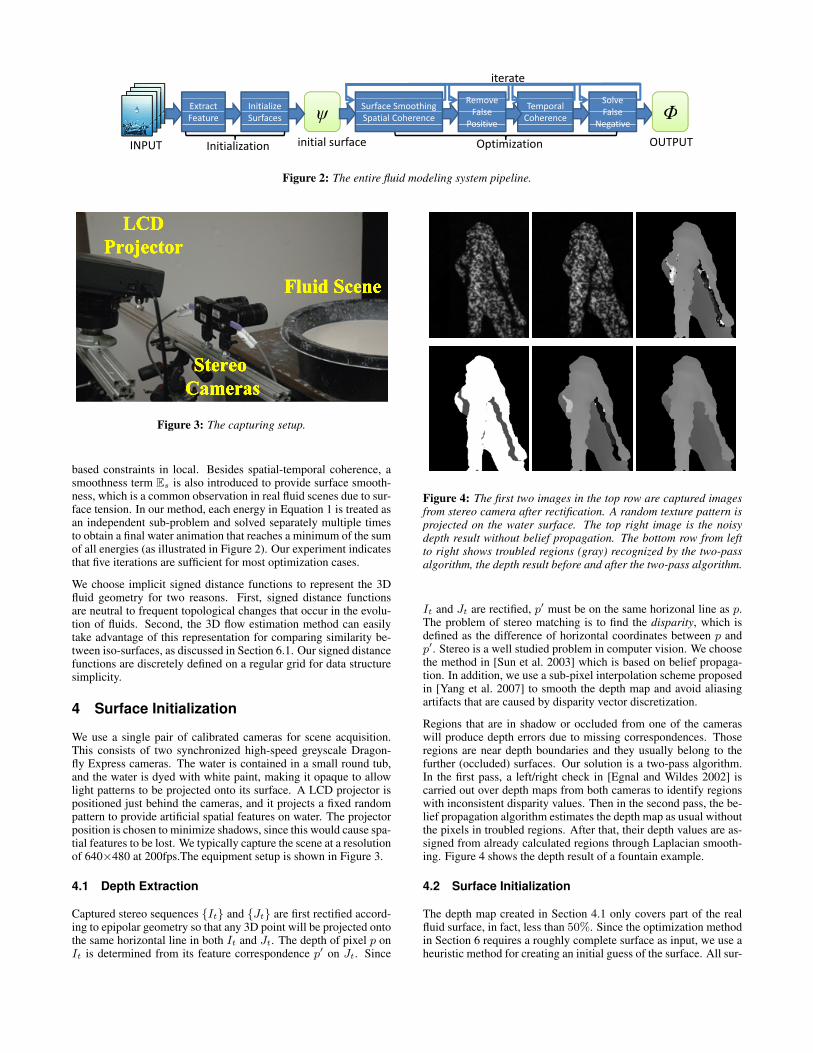
3 Overview

Given a video sequence captured by a synchronized, calibratedstereo camera system, the goal of our hybrid water modeling tech-nique is to efficiently reconstruct realistic 3D fluid animations withphysical soundness. Our framework consists of two stages as shownin Figure 2. Let {It} and {Jt} be video sequences captured bystereo camera at time t ∈ [0, T ]. In the first stage, an initial shapesequence Ψ = {ψi} is assembled by reconstructing each frame in-dependently using depth from stereo. Ψ is then optimized in thesecond stage to generate a shape sequence Φ = {φi} that satisfiesspatial-temporal coherence.

Spatial coherence means that Φ should be similar to the captureddata input Ψ. Temporal coherence means that Φ should satisfy thebehavior of fluids as much as possible. Mathematically, this is inter-preted as the minimum solution to the following energy functional:

E(Φ) =

T∑t=0

(Ed(φt, ψt) + Es(φt)) +

T−1∑t=0

En(φt, φt+1) (1)

Here Ed(φt, ψt) calculates the similarity between φt and ψt, andEn(φt, φt+1) measures how closely Φ satisfies the physically-

iterateiterate

R S lExtract Initialize

RemoveTemporal

SolveSurface SmoothingExtract  ψInitialize 

FalseTemporal 

False ΦSurface SmoothingFeature ψSurfaces

FalseCoherence

False ΦSpatial CoherenceFeature ψSurfaces Positive

CoherenceNegative

ΦSpatial CoherencePositive Negative

l fINPUT OUTPUTinitial surfaceInitialization OptimizationINPUT OUTPUTinitial surfaceInitialization Optimization

Figure 2: The entire fluid modeling system pipeline.

LCDProjector

Fluid Scene

Stereo Cameras

Figure 3: The capturing setup.

based constraints in local. Besides spatial-temporal coherence, asmoothness term Es is also introduced to provide surface smooth-ness, which is a common observation in real fluid scenes due to sur-face tension. In our method, each energy in Equation 1 is treated asan independent sub-problem and solved separately multiple timesto obtain a final water animation that reaches a minimum of the sumof all energies (as illustrated in Figure 2). Our experiment indicatesthat five iterations are sufficient for most optimization cases.

We choose implicit signed distance functions to represent the 3Dfluid geometry for two reasons. First, signed distance functionsare neutral to frequent topological changes that occur in the evolu-tion of fluids. Second, the 3D flow estimation method can easilytake advantage of this representation for comparing similarity be-tween iso-surfaces, as discussed in Section 6.1. Our signed distancefunctions are discretely defined on a regular grid for data structuresimplicity.

4 Surface Initialization

We use a single pair of calibrated cameras for scene acquisition.This consists of two synchronized high-speed greyscale Dragon-fly Express cameras. The water is contained in a small round tub,and the water is dyed with white paint, making it opaque to allowlight patterns to be projected onto its surface. A LCD projector ispositioned just behind the cameras, and it projects a fixed randompattern to provide artificial spatial features on water. The projectorposition is chosen to minimize shadows, since this would cause spa-tial features to be lost. We typically capture the scene at a resolutionof 640×480 at 200fps.The equipment setup is shown in Figure 3.

4.1 Depth Extraction

Captured stereo sequences {It} and {Jt} are first rectified accord-ing to epipolar geometry so that any 3D point will be projected ontothe same horizontal line in both It and Jt. The depth of pixel p onIt is determined from its feature correspondence p′ on Jt. Since

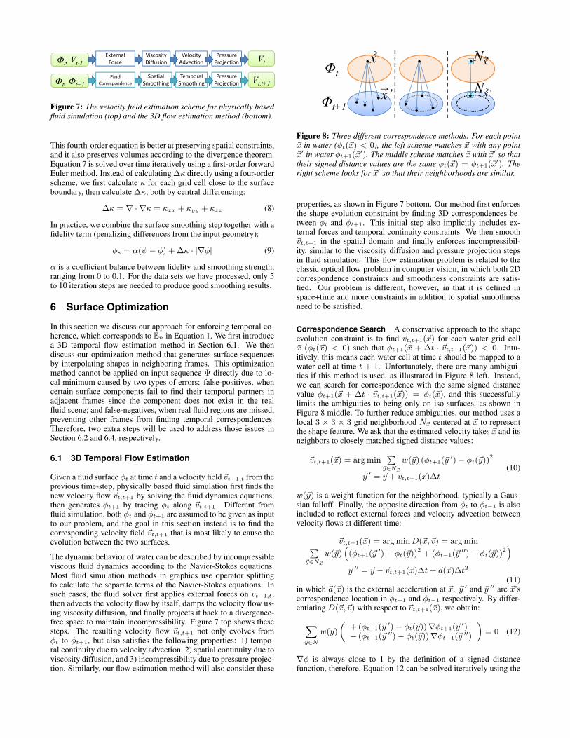
Figure 4: The first two images in the top row are captured imagesfrom stereo camera after rectification. A random texture pattern isprojected on the water surface. The top right image is the noisydepth result without belief propagation. The bottom row from leftto right shows troubled regions (gray) recognized by the two-passalgorithm, the depth result before and after the two-pass algorithm.

It and Jt are rectified, p′ must be on the same horizonal line as p.The problem of stereo matching is to find the disparity, which isdefined as the difference of horizontal coordinates between p andp′. Stereo is a well studied problem in computer vision. We choosethe method in [Sun et al. 2003] which is based on belief propaga-tion. In addition, we use a sub-pixel interpolation scheme proposedin [Yang et al. 2007] to smooth the depth map and avoid aliasingartifacts that are caused by disparity vector discretization.

Regions that are in shadow or occluded from one of the cameraswill produce depth errors due to missing correspondences. Thoseregions are near depth boundaries and they usually belong to thefurther (occluded) surfaces. Our solution is a two-pass algorithm.In the first pass, a left/right check in [Egnal and Wildes 2002] iscarried out over depth maps from both cameras to identify regionswith inconsistent disparity values. Then in the second pass, the be-lief propagation algorithm estimates the depth map as usual withoutthe pixels in troubled regions. After that, their depth values are as-signed from already calculated regions through Laplacian smooth-ing. Figure 4 shows the depth result of a fountain example.

4.2 Surface Initialization

The depth map created in Section 4.1 only covers part of the realfluid surface, in fact, less than 50%. Since the optimization methodin Section 6 requires a roughly complete surface as input, we use aheuristic method for creating an initial guess of the surface. All sur-

faces starting from this point on are represented as signed distancefunctions on a regular volumetric grid.

Using Γt, the partial surface defined according to the depth mapat time t, an initial surface ψt can be created by the union of allspheres centered at Γt with radius r:

ψt(~x) = miny∈Γt

(‖~x− ~y‖ − r) (2)

This method is effective when the water behaves like a thin shellor film, as our pouring example in Figure 12. It is not sufficientwhen large water regions are missing due to occlusion, therefore,simple heuristics are used in our experiments to approximate themissing region. For instance, the splash example of Figure 14 isnearly symmetric to a vertical plane z = z0. We first fill in thewater volume beneath the visible surface as a height field. Let ~y bethe lowest point in Γt on the same vertical line as a grid cell ~x:

~y = arg min ~yy (~y ∈ Γt, (~y − ~x) ‖ Y axis ) (3)

For any ~x whose ~y exists, its signed distance value is simply:

ψt(~x) = ~yy − ~xy (4)

If ~x doesn’t have ~y but its symmetric counterpart ~x′ = ~x+ (2z0 −~xy)(0, 1, 0)T to the plane has a ~y′ defined, the signed distance canthen be copied from its counterpart as: ψt(~x) = ψt(~x

′). Finally,the value for the rest undefined grid cells are blended from its fourhorizontal neighbors to complete the surface ψt. An example isshown in Figure 5.

Space-Time Merging When a water scene exhibits temporalrepetitiveness rather than spatial repetitiveness, similar ideas canbe applied to reconstruct the initial shape ψt using video sequencescaptured at different time from different viewpoint. For example, asingle pair of cameras is unable to simultaneously capture both thedownstream (front) and the upstream (back) in our fountain casein Figure 6 due to occlusions. Our solution is to capture each ofthese streams in turn, e.g., first capture the upstream view, thanmove the camera around to capture the downstream view. Whileeach surface immediately generated from video cannot cover thewhole fluid surface, they can be stitched together assuming that thetemporal repetition gives a similar dynamic appearance over time.First the relative camera pose of each view can be found using staticpoints (fiducials) in the scene. From the pose information, differ-ent sequences can be aligned. Note that this alignment does notrequire high-accuracy, even slightly moving points can be used asfiducials. If original sequences are sufficiently long, we choose twooptimal sub-sequences from the original input such that the over-all difference between them are minimized after spatial alignment.The shape difference is measured as the sum-of-squared differencebetween two signed distance functions. Although the resulting sur-face ψt may not correspond exactly to a real water scene, our exper-iment shows that this approach produces visually plausible results.

5 Surface Smoothing and Spatial Coherence

Real fluid surfaces are smooth in space due to the effect of surfacetension, especially for water at small scales. To provide similarresults in our method, we use a surface smoothing scheme eachtime the surface sequence is updated.

Mean curvature flow can provide a surface smoothing effect, andthis can be achieved using the following level set formulation:

φs = κ · |∇φ| (5)

z

z=z0

Figure 5: The initialization result for the splash example. Fromleft to right and top to bottom are the partial surface Γt from thedepth map, surface after initialization, surface after initializationand smoothing, and the final reconstructed surface respectively.

Figure 6: While each surface reconstructed solely in the front view(left) or back view (middle) cannot cover the whole surface, a rea-sonable initial surface can be generated by assembling two viewstogether, even if they are captured at different time.

in which s → ∞, standing for a steady solution. κ is the surfacemean curvature.The mean curvature flow tries to minimize the sur-face area by making mean curvature uniform over the whole sur-face, so that the tendency is for the surface to evolve towards aspherical shape. Using such a level-set mean curvature evolution isstraightforward to implement, but it performs excessive smoothingand does not take into account fidelity to the original geometry (ourspatial constraints). In fact, although the surface tension effect issimilar to the mean curvature flow over time, temporal surface ten-sion distribution on a time-varying surface is not the steady state ofthe mean curvature flow. Instead, we choose the smoothing schemeproposed by Schneider and Kobbelt [2001] under the following tar-get PDE:

∆Bκ(~x) = 0 (6)

∆B is the Laplacian-Beltrami operator. Assuming that κ along thesurface normal over iso-surfaces is locally linear, ∆B can be ap-proximated by a Laplacian operator in 3D, and the solution is anevolution equation in fourth order:

φs = ∆κ · |∇φ| (7)

Intuitively, this will produce a fluid surface with C2 continuousmean curvature, leading to aC2 surface tension field on the surface.

Φt, Vt-1Viscosity Diffusion

Velocity Advection

Pressure Projection

External Force Vt

Φt, Φt+1Spatial

SmoothingTemporal Smoothing

Pressure Projection

Find Correspondence Vt,t+1

Figure 7: The velocity field estimation scheme for physically basedfluid simulation (top) and the 3D flow estimation method (bottom).

This fourth-order equation is better at preserving spatial constraints,and it also preserves volumes according to the divergence theorem.Equation 7 is solved over time iteratively using a first-order forwardEuler method. Instead of calculating ∆κ directly using a four-orderscheme, we first calculate κ for each grid cell close to the surfaceboundary, then calculate ∆κ, both by central differencing:

∆κ = ∇ · ∇κ = κxx + κyy + κzz (8)

In practice, we combine the surface smoothing step together with afidelity term (penalizing differences from the input geometry):

φs = α(ψ − φ) + ∆κ · |∇φ| (9)

α is a coefficient balance between fidelity and smoothing strength,ranging from 0 to 0.1. For the data sets we have processed, only 5to 10 iteration steps are needed to produce good smoothing results.

6 Surface Optimization

In this section we discuss our approach for enforcing temporal co-herence, which corresponds to En in Equation 1. We first introducea 3D temporal flow estimation method in Section 6.1. We thendiscuss our optimization method that generates surface sequencesby interpolating shapes in neighboring frames. This optimizationmethod cannot be applied on input sequence Ψ directly due to lo-cal minimum caused by two types of errors: false-positives, whencertain surface components fail to find their temporal partners inadjacent frames since the component does not exist in the realfluid scene; and false-negatives, when real fluid regions are missed,preventing other frames from finding temporal correspondences.Therefore, two extra steps will be used to address those issues inSection 6.2 and 6.4, respectively.

6.1 3D Temporal Flow Estimation

Given a fluid surface φt at time t and a velocity field ~vt−1,t from theprevious time-step, physically based fluid simulation first finds thenew velocity flow ~vt,t+1 by solving the fluid dynamics equations,then generates φt+1 by tracing φt along ~vt,t+1. Different fromfluid simulation, both φt and φt+1 are assumed to be given as inputto our problem, and the goal in this section instead is to find thecorresponding velocity field ~vt,t+1 that is most likely to cause theevolution between the two surfaces.

The dynamic behavior of water can be described by incompressibleviscous fluid dynamics according to the Navier-Stokes equations.Most fluid simulation methods in graphics use operator splittingto calculate the separate terms of the Navier-Stokes equations. Insuch cases, the fluid solver first applies external forces on vt−1,t,then advects the velocity flow by itself, damps the velocity flow us-ing viscosity diffusion, and finally projects it back to a divergence-free space to maintain incompressibility. Figure 7 top shows thesesteps. The resulting velocity flow ~vt,t+1 not only evolves fromφt to φt+1, but also satisfies the following properties: 1) tempo-ral continuity due to velocity advection, 2) spatial continuity due toviscosity diffusion, and 3) incompressibility due to pressure projec-tion. Similarly, our flow estimation method will also consider these

xΦt

Nx

x’Φt+1Nx’

t 1

Figure 8: Three different correspondence methods. For each point~x in water (φt(~x) < 0), the left scheme matches ~x with any point~x′ in water φt+1(~x

′). The middle scheme matches ~x with ~x′ so thattheir signed distance values are the same φt(~x) = φt+1(~x

′). Theright scheme looks for ~x′ so that their neighborhoods are similar.

properties, as shown in Figure 7 bottom. Our method first enforcesthe shape evolution constraint by finding 3D correspondences be-tween φt and φt+1. This initial step also implicitly includes ex-ternal forces and temporal continuity constraints. We then smooth~vt,t+1 in the spatial domain and finally enforces incompressibil-ity, similar to the viscosity diffusion and pressure projection stepsin fluid simulation. This flow estimation problem is related to theclassic optical flow problem in computer vision, in which both 2Dcorrespondence constraints and smoothness constraints are satis-fied. Our problem is different, however, in that it is defined inspace+time and more constraints in addition to spatial smoothnessneed to be satisfied.

Correspondence Search A conservative approach to the shapeevolution constraint is to find ~vt,t+1(~x) for each water grid cell~x (φt(~x) < 0) such that φt+1(~x + ∆t · ~vt,t+1(~x)) < 0. Intu-itively, this means each water cell at time t should be mapped to awater cell at time t + 1. Unfortunately, there are many ambigui-ties if this method is used, as illustrated in Figure 8 left. Instead,we can search for correspondence with the same signed distancevalue φt+1(~x + ∆t · ~vt,t+1(~x)) = φt(~x), and this successfullylimits the ambiguities to being only on iso-surfaces, as shown inFigure 8 middle. To further reduce ambiguities, our method uses alocal 3 × 3 × 3 grid neighborhood N~x centered at ~x to representthe shape feature. We ask that the estimated velocity takes ~x and itsneighbors to closely matched signed distance values:

~vt,t+1(~x) = arg min∑

~y∈N~x

w(~y) (φt+1(~y′)− φt(~y))

2

~y ′ = ~y + ~vt,t+1(~x)∆t(10)

w(~y) is a weight function for the neighborhood, typically a Gaus-sian falloff. Finally, the opposite direction from φt to φt−1 is alsoincluded to reflect external forces and velocity advection betweenvelocity flows at different time:

~vt,t+1(~x) = arg minD(~x,~v) = arg min∑~y∈N~x

w(~y)((φt+1(~y

′)− φt(~y))2

+ (φt−1(~y′′)− φt(~y))

2)

~y ′′ = ~y − ~vt,t+1(~x)∆t+ ~a(~x)∆t2

(11)in which ~a(~x) is the external acceleration at ~x. ~y ′ and ~y ′′ are ~x’scorrespondence location in φt+1 and φt−1 respectively. By differ-entiating D(~x,~v) with respect to ~vt,t+1(~x), we obtain:

∑~y∈N

w(~y)

(+ (φt+1(~y

′)− φt(~y))∇φt+1(~y′)

− (φt−1(~y′′)− φt(~y))∇φt−1(~y

′′)

)= 0 (12)

∇φ is always close to 1 by the definition of a signed distancefunction, therefore, Equation 12 can be solved iteratively using the

Newton-Ralphson method. ~v(~x) can be initialized with zeros, sev-eral candidate seeds from heuristics, or user estimation if available.For each iteration, a new velocity flow ~vnew(~x) is calculated fromthe old one ~vold(~x):∑

~y∈N

w(~y)

(+ (φt+1(~y

′new)− φt(~y))∇φt+1(~y

′old)

− (φt−1(~y′′new)− φt(~y))∇φt−1(~y

′′old)

)= 0

(13)~y′new, ~y

′′new and ~y′old, ~y

′′old are ~y’s correspondences calculated us-

ing new and old velocity flows respectively. We further linearizeφt+1(~y

′new) and φt−1(~y

′′new) as:

φt+1(~y′new) ≈ φt+1(~y

′old) +∇φT

t+1(~y′old)(~vnew − ~vold)∆t

φt−1(~y′′new) ≈ φt−1(~y

′′old)−∇φT

t+1(~y′′old)(~vnew − ~vold)∆t

(14)Combining Equation 13 with 14 gives us a linear system with~vnew(~x) as unknowns. Iterations are terminated if maximum it-eration number is reached or if ~vnew − ~vold drops below certainthreshold (0.05 of a grid cell size in our experiments). We alsolimit |~vnew − ~vold| by an upper bound for smoother convergence.We also limit the search space within a range around the initialguess to prevent large velocity changes in case the problem is ill-conditioned. This solution is similar to the classic Kanade-Lucas-Tomasi (KLT) feature tracker [Shi and Tomasi 1994] with transla-tion motions only, except that our problem is defined in 3D and thesearch procedure considers both forward and backward directions.

When two separate water regions merge or split, this estimationscheme may not work for all grid cells. For instance, a grid cellmay not find its actual correspondence according to the neighbor-hood similarity in Equation 11, when it represents a water dropdripping into a still water surface. Similar to the aperture problemin KLT, this scheme also fails to work when the fluid shape barelychanges, i.e., a static flow. Fortunately, both problems can be solvedusing smoothness and incompressibility constraints by propagatingcorrectly estimated flows into ill-defined regions, as will be dis-cussed next. Figure 9 shows a frame in a water splash example andits estimated velocity field using this algorithm.

If the correspondence search in one direction goes beyond thespatial-temporal boundary, we assume that everything is possibleoutside of the 4D space-time grid, and the corresponding error inEquation 11 and correction in 13 are simply ignored.

Error Measure D(~x,~v) in Equation 11 is used as an error mea-sure to determine whether ~x’s correspondence exists in the neigh-boring frame. If D is below some tolerance ε at time t, we catego-rize ~x at time t as Type-I , which means it has correspondences inboth φt−1 and φt+1. Otherwise, the method will try to locate cor-respondences only in φt−1 or φt+1, with half of the tolerance ε/2.We do this by removing the error and correction contribution fromthe other neighboring frame in Equation 11 and 13. Grid cells willbe type-II if correspondence exists in φt+1, or type-III , if cor-respondence exists in φt−1. The rest of grid cells will be type-O,which means no correspondence is found in either φt−1 or φt+1.

Spatial Smoothing The spatial smoothing step here mimics theviscosity effect, similar to using an explicit solver by discretizingthe Laplacian operator for viscosity effects:

~vt,t+1(~x) =∑

s(~y)~vt,t+1(~y) (15)

~y is a water grid cell within an immediate grid neighborhood of ~x,including ~x and its six neighbors. Typically, s(~y) defines the spatialsmoothing kernel covering ~p and its six immediate neighbors as:

s(~y) = 1− 6β (~y = ~x), s(~y) = β (otherwise) (16)

Figure 9: One frame in a water splash example and its estimatedvelocity field visualizated as a vector diagram.

β is specified by user according to their expectation of velocityspatial smoothness. It should be noted that although this methodlooks similar to the explicit viscosity solver in physically basedfluid solver, it only provides similar effect as viscosity diffusionand it is not based on actually fluid dynamics since only a staticvelocity field is involved.

To generate large viscosity effect, some fluid simulation algo-rithms [Stam 1999; Carlson et al. 2002] formulate viscosity dif-fusion implicitly as a sparse linear system. Our method choosesto simply apply the smoothing process multiple times to produce avisually plausible velocity flow.

Pressure Projection While the velocity is defined at each gridcell for the convenience of estimation and optimization, it is notstraightforward to couple velocity with pressure, which is also de-fined at the grid cell. Our simple solution is to first interpolate thevelocity flow to a staggered grid formulation by averaging, then ap-ply pressure projection, and convert the velocity back to the gridcell center. Details about the pressure projection in a staggeredMark-and-Cell (MAC) grid can be found in [Stam 1999]. We useDirichlet boundary condition with zero outer pressure when waterbodies are completely within the space-time grid. Water bodies ex-panding beyond the space-time grid are ignored in this step sincetheir volumes outside of the grid are unknown.

After the pressure projection step, error scores are recalculated andgrid cells are re-categorized. This category information will be usedto determine whether missing correspondence is caused by false-positives or false-negatives.

6.2 False-Positive Removal

Since both false-positives and false-negatives can cause missingcorrespondences in neighboring frames, the first task is to deter-mine the cause of a missing correspondence. We do this by count-ing how many consecutive frames a water region appears in, as-suming that real water should at least exists in several consecutiveframes. For example, when a water region only appears in framet, or frame t and t + 1, it is less likely to be a water component inthe real scene. However, if it exists in more frames, missing cor-respondences are more likely to be caused by false-negatives, sothe component should not be removed. This assumption fails incertain cases, for example, a water drop intermittently missing in a

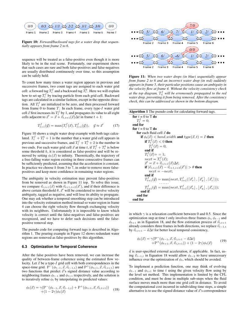
Figure 10: Forward/backward tags for a water drop that sequen-tially appears from frame 2 to 6.

sequence will be treated as a false-positive even though it is morelikely to be in the real scene. Fortunately, our experiment showsthat such cases are rare and both false-positives and false-negativesare usually distributed continuously over time, so this assumptioncan be safely held.

To count how many times a water region appears in previous andsuccessive frames, two count tags are assigned to each water gridcell: a forward tag T f

t and a backward tag T bt . Here we will explain

how to set up T ft by tracing particle from each grid cell. Backward

tags are calculated in a similar fashion, except in the opposite direc-tion. All T f

t are initialized to be zero, and then processed forwardfrom frame 0 to frame T . In each frame, every type-I water gridcell ~x first increases its T f

t by 1, and propagates its value to all eightcells adjacent to ~x′ = ~x+ ~vt,t+1(~x)∆t in frame t+ 1:

T ft+1(~y) = max(T f

t (~x), T ft+1(~y)), ~y ≈ ~x′ (17)

Figure 10 shows a single water drop example with both tags calcu-lated. T f

t + T bt + 1 is the number that a water grid cell appears in

previous and successive frames, and T ft + T b

t + 2 is the number intwo ends. For each water grid cell ~x at time t, if T f

t + T bt is below

some threshold k, it is considered as false-positive and will be re-moved by setting φt(~x) to infinity. Theoretically, the trajectory ofa free-falling water region existing in three consecutive frames canbe sufficiently predicted, assuming that the acceleration is constant.In practice we choose k from 3 to 7, in order to remove more false-positives and keep more confidence in remaining water regions.

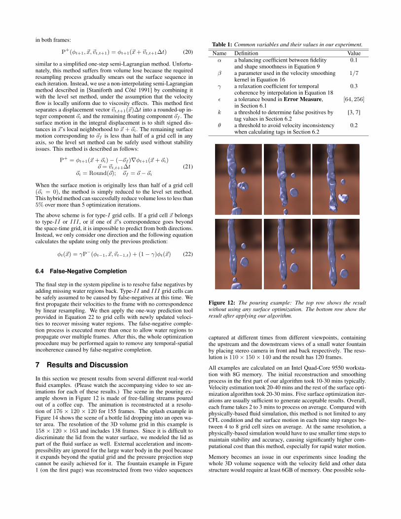
The ambiguity in velocity estimation may prevent false-positivesfrom be removed as shown in Figure 11 top. To solve this issue,we compare ~vt,t+1(~x) with ~vt+1,t+2(~x

′), and if their difference isabove certain threshold θ, ~x′ will be considered to involve velocityambiguity, tagged as negative, and will lose its ability to propagate.One may ask whether a temporal smoothing step can be introducedinto the velocity estimation method instead so water region in frame4 can choose the right velocity flow through exchanging velocitywith its neighbors. Unfortunately it is impossible to know whichvelocity is correct until the false-negatives and false-positives arerecognized, and we have to defer such decisions until the false-positive removal step.

The pseudo code for computing forward tags is described in Algo-rithm 1. The pouring example in Figure 12 shows redundant waterregions are removed as false-positives by this algorithm.

6.3 Optimization for Temporal Coherence

After the false positives have been removed, we can increase thequality of between-frame coherence using the estimated flow ve-locity. Let ~x be a type-I grid cell with both correspondences in thespace-time grid. P−(φt−1, ~x,~vt−1,t) and P+(φt+1, ~x,~vt,t+1) aretwo functions that predict ~x’s signed distance value according toneighboring frames φt−1 and φt+1 respectively, and the solution isto iteratively refine φt by interpolating its predicted values:

φt(~x) = γ(P−(φt−1, ~x,~vt−1,t) + P+(φt+1, ~x,~vt,t+1))+(1− 2γ)φt(~x)

(18)

Figure 11: When two water drops (in blue) sequentially appearfrom frame 2 to 6 and an incorrect water drop (in red) suddenlyappears in frame 5, their particular positions cause an ambiguity inthe velocity flow at frame 4. Without the velocity consistency checkat the top diagram, T f

4 will be erroneously propagated to the redwater drop, preventing it from being removed. After the consistencycheck, this can be addressed as shown in the bottom diagram.

Algorithm 1 The pseudo code for calculating forward tags.for t = 0 to T doT f

t = 0;end forfor t = 0 to T do

for each fluid cell ~x doif φt(~x) < band width and type(~x, t) = I then

if T ft (~x) < 0 thenT f

t (~x) = 0;end ifT f

t (~x)+ = 1;next = T f

t (~x);~x′ = ~x+ ~vt,t+1(~x)∆t;if |~vt,t+1(~x)− ~vi+1,i+2(~x

′)| > θ thennext = −next;

end ifT f

t+1(~y) = max(next, T ft+1(d~x′xe ,

⌈~x′y

⌉, d~x′ze));

· · · · · ·T f

t+1(~y) = max(next, T ft+1(b~x′xc ,

⌊~x′y

⌋, b~x′zc));

end ifend for

end for

in which γ is a relaxation coefficient between 0 and 0.5. Since theoptimization step at time t only involves three frames φt, φt−1 andφt+1 as in Equation 18, and the flow estimation process of ~vt,t+1

already considers three frames in both directions, we replace ~vt−1,t

by ~vt,t+1 − ~a∆t for better local temporal consistency,

φt(~x) = γ(P−(φt−1, ~x,~vt,t+1 − ~a∆t)+P+(φt+1, ~x,~vt,t+1)) + (1− 2γ)φt(~x)

(19)

~a is user-specified external acceleration, if applicable. In fact, us-ing ~vt−1,t in Equation 18 would allow φt−2 to have unnecessaryinfluence over the optimization of φt, which should be avoided.

To implement a prediction function, one may think of evolvingφt−1 and φt+1 to time t using the given velocity flow using bythe level set method. This implementation is limited by the CFLcondition, and must be done in multiple sub-steps when the fluidsurface moves much more than one grid cell in distance. To avoidthe computational cost incurred in subdividing time steps, a simplealternative is to use the signed distance value of ~x’s correspondence

in both frames:

P+(φt+1, ~x,~vt,t+1) = φt+1(~x+ ~vt,t+1∆t) (20)

similar to a simplified one-step semi-Lagrangian method. Unfortu-nately, this method suffers from volume lose because the requiredresampling process gradually smears out the surface sequence ineach iteration. Instead, we use a non-interpolating semi-Lagrangianmethod described in [Staniforth and Cote 1991] by combining itwith the level set method, under the assumption that the velocityflow is locally uniform due to viscosity effects. This method firstseparates a displacement vector ~vt,t+1(~x)∆t into a rounded-up in-teger component ~oi and the remaining floating component ~of . Thesurface motion in the integral displacement is to shift signed dis-tances in ~x’s local neighborhood to ~x + ~oi. The remaining surfacemotion corresponding to ~of is less than half of a grid cell in anyaxis, so the level set method can be safely used without stabilityissues. This method is described as follows:

P+ = φt+1(~x+ ~oi)− (−~of )∇φt+1(~x+ ~oi)~o = ~vt,t+1∆t

~oi = Round(~o); ~of = ~o− ~oi

(21)

When the surface motion is originally less than half of a grid cell(~oi = 0), the method is simply reduced to the level set method.This hybrid method can successfully reduce volume loss to less than5% over more than 5 optimization iterations.

The above scheme is for type-I grid cells. If a grid cell ~x belongsto type-II or III , or if one of ~x’s correspondence goes beyondthe space-time grid, it is impossible to predict from both directions.Instead, we only consider one direction and the following equationcalculates the update using only the previous prediction:

φt(~x) = γP−(φt−1, ~x,~vt−1,t) + (1− γ)φt(~x) (22)

6.4 False-Negative Completion

The final step in the system pipeline is to resolve false negatives byadding missing water regions back. Type-II and III grid cells canbe safely assumed to be caused by false-negatives at this time. Wefirst propagate their velocities to the frame with no correspondenceby linear resampling. We then apply the one-way prediction toolprovided in Equation 22 to grid cells with newly updated veloci-ties to recover missing water regions. The false-negative comple-tion process is executed more than once to allow water regions topropagate over multiple frames. After this, the whole optimizationprocedure may be performed again to remove any temporal-spatialincoherence caused by false-negative completion.

7 Results and Discussion

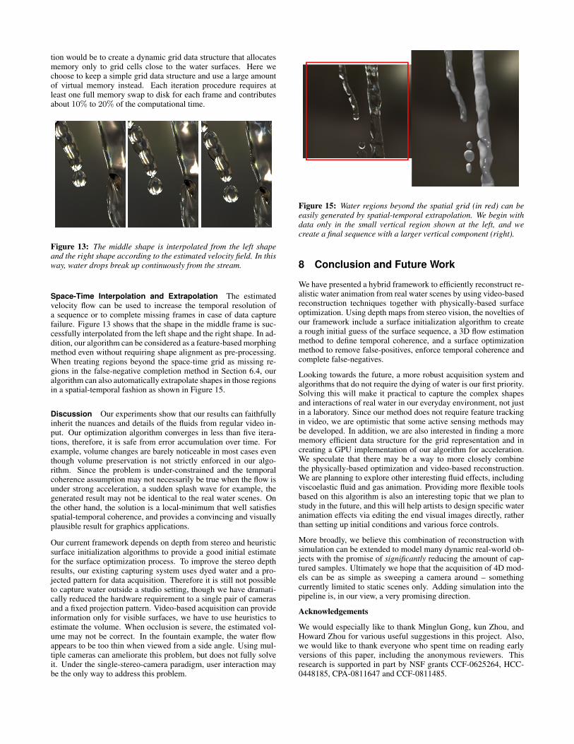
In this section we present results from several different real-worldfluid examples. (Please watch the accompanying video to see an-imations for each of these results.) The scene in the pouring ex-ample shown in Figure 12 is made of free-falling streams pouredout of a coffee cup. The animation is reconstructed at a resolu-tion of 176 × 120 × 120 for 155 frames. The splash example inFigure 14 shows the scene of a bottle lid dropping into an open wa-ter area. The resolution of the 3D volume grid in this example is158 × 120 × 163 and includes 138 frames. Since it is difficult todiscriminate the lid from the water surface, we modeled the lid aspart of the fluid surface as well. External acceleration and incom-pressibility are ignored for the large water body in the pool becauseit expands beyond the spatial grid and the pressure projection stepcannot be easily achieved for it. The fountain example in Figure1 (on the first page) was reconstructed from two video sequences

Table 1: Common variables and their values in our experiment.Name Definition Valueα a balancing coefficient between fidelity 0.1

and shape smoothness in Equation 9β a parameter used in the velocity smoothing 1/7

kernel in Equation 16γ a relaxation coefficient for temporal 0.3

coherence by interpolation in Equation 18ε a tolerance bound in Error Measure, [64, 256]

in Section 6.1k a threshold to determine false positives by [3, 7]

tag values in Section 6.2θ a threshold to avoid velocity inconsistency 0.2

when calculating tags in Section 6.2

Figure 12: The pouring example: The top row shows the resultwithout using any surface optimization. The bottom row show theresult after applying our algorithm.

captured at different times from different viewpoints, containingthe upstream and the downstream views of a small water fountainby placing stereo camera in front and back respectively. The reso-lution is 110× 150× 140 and the result has 120 frames.

All examples are calculated on an Intel Quad-Core 9550 worksta-tion with 8G memory. The initial reconstruction and smoothingprocess in the first part of our algorithm took 10-30 mins typically.Velocity estimation took 20-40 mins and the rest of the surface opti-mization algorithm took 20-30 mins. Five surface optimization iter-ations are usually sufficient to generate acceptable results. Overall,each frame takes 2 to 3 mins to process on average. Compared withphysically-based fluid simulation, this method is not limited to anyCFL condition and the surface motion in each time step ranges be-tween 4 to 8 grid cell sizes on average. At the same resolution, aphysically-based simulation would have to use smaller time steps tomaintain stability and accuracy, causing significantly higher com-putational cost than this method, especially for rapid water motion.

Memory becomes an issue in our experiments since loading thewhole 3D volume sequence with the velocity field and other datastructure would require at least 6GB of memory. One possible solu-

tion would be to create a dynamic grid data structure that allocatesmemory only to grid cells close to the water surfaces. Here wechoose to keep a simple grid data structure and use a large amountof virtual memory instead. Each iteration procedure requires atleast one full memory swap to disk for each frame and contributesabout 10% to 20% of the computational time.

Figure 13: The middle shape is interpolated from the left shapeand the right shape according to the estimated velocity field. In thisway, water drops break up continuously from the stream.

Space-Time Interpolation and Extrapolation The estimatedvelocity flow can be used to increase the temporal resolution ofa sequence or to complete missing frames in case of data capturefailure. Figure 13 shows that the shape in the middle frame is suc-cessfully interpolated from the left shape and the right shape. In ad-dition, our algorithm can be considered as a feature-based morphingmethod even without requiring shape alignment as pre-processing.When treating regions beyond the space-time grid as missing re-gions in the false-negative completion method in Section 6.4, ouralgorithm can also automatically extrapolate shapes in those regionsin a spatial-temporal fashion as shown in Figure 15.

Discussion Our experiments show that our results can faithfullyinherit the nuances and details of the fluids from regular video in-put. Our optimization algorithm converges in less than five itera-tions, therefore, it is safe from error accumulation over time. Forexample, volume changes are barely noticeable in most cases eventhough volume preservation is not strictly enforced in our algo-rithm. Since the problem is under-constrained and the temporalcoherence assumption may not necessarily be true when the flow isunder strong acceleration, a sudden splash wave for example, thegenerated result may not be identical to the real water scenes. Onthe other hand, the solution is a local-minimum that well satisfiesspatial-temporal coherence, and provides a convincing and visuallyplausible result for graphics applications.

Our current framework depends on depth from stereo and heuristicsurface initialization algorithms to provide a good initial estimatefor the surface optimization process. To improve the stereo depthresults, our existing capturing system uses dyed water and a pro-jected pattern for data acquisition. Therefore it is still not possibleto capture water outside a studio setting, though we have dramati-cally reduced the hardware requirement to a single pair of camerasand a fixed projection pattern. Video-based acquisition can provideinformation only for visible surfaces, we have to use heuristics toestimate the volume. When occlusion is severe, the estimated vol-ume may not be correct. In the fountain example, the water flowappears to be too thin when viewed from a side angle. Using mul-tiple cameras can ameliorate this problem, but does not fully solveit. Under the single-stereo-camera paradigm, user interaction maybe the only way to address this problem.

Figure 15: Water regions beyond the spatial grid (in red) can beeasily generated by spatial-temporal extrapolation. We begin withdata only in the small vertical region shown at the left, and wecreate a final sequence with a larger vertical component (right).

8 Conclusion and Future Work

We have presented a hybrid framework to efficiently reconstruct re-alistic water animation from real water scenes by using video-basedreconstruction techniques together with physically-based surfaceoptimization. Using depth maps from stereo vision, the novelties ofour framework include a surface initialization algorithm to createa rough initial guess of the surface sequence, a 3D flow estimationmethod to define temporal coherence, and a surface optimizationmethod to remove false-positives, enforce temporal coherence andcomplete false-negatives.

Looking towards the future, a more robust acquisition system andalgorithms that do not require the dying of water is our first priority.Solving this will make it practical to capture the complex shapesand interactions of real water in our everyday environment, not justin a laboratory. Since our method does not require feature trackingin video, we are optimistic that some active sensing methods maybe developed. In addition, we are also interested in finding a morememory efficient data structure for the grid representation and increating a GPU implementation of our algorithm for acceleration.We speculate that there may be a way to more closely combinethe physically-based optimization and video-based reconstruction.We are planning to explore other interesting fluid effects, includingviscoelastic fluid and gas animation. Providing more flexible toolsbased on this algorithm is also an interesting topic that we plan tostudy in the future, and this will help artists to design specific wateranimation effects via editing the end visual images directly, ratherthan setting up initial conditions and various force controls.

More broadly, we believe this combination of reconstruction withsimulation can be extended to model many dynamic real-world ob-jects with the promise of significantly reducing the amount of cap-tured samples. Ultimately we hope that the acquisition of 4D mod-els can be as simple as sweeping a camera around – somethingcurrently limited to static scenes only. Adding simulation into thepipeline is, in our view, a very promising direction.

Acknowledgements

We would especially like to thank Minglun Gong, kun Zhou, andHoward Zhou for various useful suggestions in this project. Also,we would like to thank everyone who spent time on reading earlyversions of this paper, including the anonymous reviewers. Thisresearch is supported in part by NSF grants CCF-0625264, HCC-0448185, CPA-0811647 and CCF-0811485.

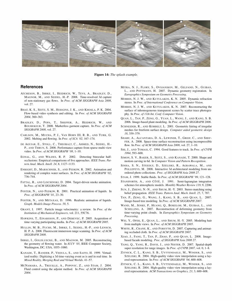
Figure 14: The splash example.

ReferencesATCHESON, B., IHRKE, I., HEIDRICH, W., TEVS, A., BRADLEY, D.,

MAGNOR, M., AND SEIDEL, H.-P. 2008. Time-resolved 3d captureof non-stationary gas flows. In Proc. of ACM SIGGRAPH Asia 2008,vol. 27.

BHAT, K. S., SEITZ, S. M., HODGINS, J. K., AND KHOSLA, P. K. 2004.Flow-based video synthesis and editing. In Proc. of ACM SIGGRAPH2004, 360–363.

BRADLEY, D., POPA, T., SHEFFER, A., HEIDRICH, W., ANDBOUBEKEUR, T. 2008. Markerless garment capture. In Proc. of ACMSIGGRAPH 2008, vol. 27.

CARLSON, M., MUCHA, P. J., VAN HORN III, R. B., AND TURK, G.2002. Melting and flowing. In Proc. of SCA ’02, 167–174.

DE AGUIAR, E., STOLL, C., THEOBALT, C., AHMED, N., SEIDEL, H.-P., AND THRUN, S. 2008. Performance capture from sparse multi-viewvideo. In Proc. of ACM SIGGRAPH ’08, 1–10.

EGNAL, G., AND WILDES, R. P. 2002. Detecting binocular half-occlusions: Empirical comparisons of five approaches. IEEE Trans. Pat-tern Anal. Mach. Intell. 24, 8, 1127–1133.

ENRIGHT, D., MARSCHNER, S., AND FEDKIW, R. 2002. Animation andrendering of complex water surfaces. In Proc. of ACM SIGGRAPH ’02,736–744.

FATTAL, R., AND LISCHINSKI, D. 2004. Target-driven smoke animation.In Proc. of ACM SIGGRAPH 2004.

FOSTER, N., AND FEDKIW, R. 2001. Practical animation of liquids. InProc. of SIGGRAPH ’01, 23–30.

FOSTER, N., AND METAXAS, D. 1996. Realistic animation of liquids.Graph. Models Image Process. 58, 5.

GRANT, I. 1997. Particle image velocimetry: a review. In Proc. of theInstitution of Mechanical Engineers, vol. 211, 55C76.

HAWKINS, T., EINARSSON, P., AND DEBEVEC, P. 2005. Acquisition oftime-varying participating media. In Proc. of ACM SIGGRAPH 2005.

HULLIN, M. B., FUCHS, M., IHRKE, I., SEIDEL, H.-P., AND LENSCH,H. P. A. 2008. Fluorescent immersion range scanning. In Proc. of ACMSIGGRAPH 2008.

IHRKE, I., GOLDLUECKE, B., AND MAGNOR, M. 2005. Reconstructingthe geometry of flowing water. In ICCV ’05, IEEE Computer Society,Washington, DC, USA, 1055–1060.

KANADE, T., RANDER, P., VEDULA, S., AND SAITO, H. 1999. Virtual-ized reality: Digitizing a 3d time-varying event as is and in real time. InMixed Reality, Merging Real and Virtual Worlds. 41–57.

MCNAMARA, A., TREUILLE, A., POPOVIC, Z., AND STAM, J. 2004.Fluid control using the adjoint method. In Proc. of ACM SIGGRAPH2004.

MITRA, N. J., FLORY, S., OVSJANIKOV, M., GELFAND, N., GUIBAS,L., AND POTTMANN, H. 2007. Dynamic geometry registration. InEurographics Symposium on Geometry Processing.

MORRIS, N. J. W., AND KUTULAKOS, K. N. 2005. Dynamic refractionstereo. In Proc. of International Conference on Computer Vision.

MORRIS, N. J. W., AND KUTULAKOS, K. N. 2007. Reconstructing thesurface of inhomogeneous transparent scenes by scatter trace photogra-phy. In Proc. of 11th Int. Conf. Computer Vision.

QUAN, L., TAN, P., ZENG, G., YUAN, L., WANG, J., AND KANG, S. B.2006. Image-based plant modeling. In Proc. of ACM SIGGRAPH 2006.

SCHNEIDER, R., AND KOBBELT, L. 2001. Geometric fairing of irregularmeshes for freeform surface design. Computer aided geometric design18, 359–379.

SHARF, A., ALCANTARA, D. A., LEWINER, T., GREIF, C., AND SHEF-FER, A. 2008. Space-time surface reconstruction using incompressibleflow. In Proc. of ACM SIGGRAPH Asia 2008, vol. 27, 1–10.

SHI, J., AND TOMASI, C. 1994. Good features to track. In Proc. of CVPR1994, 593–600.

SIMON, S. V., BAKER, S., SEITZ, S., AND KANADE, T. 2000. Shape andmotion carving in 6d. In Computer Vision and Pattern Recognition.

SINHA, S. N., STEEDLY, D., SZELISKI, R., AGRAWALA, M., ANDPOLLEFEYS, M. 2008. Interactive 3d architectural modeling from un-ordered photo collections. Proc. of SIGGRAPH Asia 2008 27.

STAM, J. 1999. Stable fluids. In Proc. of ACM SIGGRAPH ’99, 121–128.STANIFORTH, A., AND COTE, J. 1991. Semi-lagrangian integration

schemes for atmospheric models. Monthly Weather Review 119, 9, 2206.SUN, J., ZHENG, N.-N., AND SHUM, H.-Y. 2003. Stereo matching using

belief propagation. IEEE Trans. Pattern Anal. Mach. Intell. 25, 7, 787.TAN, P., ZENG, G., WANG, J., KANG, S. B., AND QUAN, L. 2007.

Image-based tree modeling. In Proc. of ACM SIGGRAPH 2007.WAND, M., JENKE, P., HUANG, Q., BOKELOH, M., GUIBAS, L., AND

SCHILLING, A. 2007. Reconstruction of deforming geometry fromtime-varying point clouds. In Eurographics Symposium on GeometryProcessing.

WEI, Y., OFEK, E., QUAN, L., AND SHUM, H.-Y. 2005. Modeling hairfrom multiple views. In Proc. of ACM SIGGRAPH 2005.

WHITE, R., CRANE, K., AND FORSYTH, D. 2007. Capturing and animat-ing occluded cloth. In Proc. of ACM SIGGRAPH 2007.

XIAO, J., FANG, T., TAN, P., ZHAO, P., AND QUAN, L. 2008. Image-based facade modeling. Proc. of SIGGRAPH Asia 2008 27.

YANG, Q., YANG, R., DAVIS, J., AND NISTER, D. 2007. Spatial-depthsuper resolution for range images. In Proc. of CVPR 2007, vol. 0, 1–8.

ZITNICK, C. L., KANG, S. B., UYTTENDAELE, M., WINDER, S., ANDSZELISKI, R. 2004. High-quality video view interpolation using a lay-ered representation. In Proc. of ACM SIGGRAPH ’04, 600–608.

ZITNICK, C. L., KANG, S. B., UYTTENDAELE, M., WINDER, S., ANDSZELISKI, R. 2004. High-quality video view interpolation using a lay-ered representation. ACM Transactions on Graphics, 23, 3, 600–608.