Quantum Optical Realization of Arbitrary Linear TransformationsAllowing for Loss and Gain

N. Tischler*

Centre for Quantum Dynamics, Griffith University, Brisbane 4111, Australia;Department of Physics and Astronomy, Macquarie University, Sydney 2109, Australia

and Vienna Center for Quantum Science and Technology, Faculty of Physics, University of Vienna,Boltzmanngasse 5, A-1090 Vienna, Austria

C. Rockstuhl†

Institute of Theoretical Solid State Physics, Karlsruhe Institute of Technology, 76131 Karlsruhe, Germanyand Institute of Nanotechnology, Karlsruhe Institute of Technology, 76021 Karlsruhe, Germany

K. Słowik‡

Institute of Physics, Faculty of Physics, Astronomy and Informatics, Nicolaus Copernicus University,Grudziadzka 5, 87-100 Torun, Poland

(Received 5 December 2017; published 13 April 2018)

Unitary transformations are routinely modeled and implemented in the field of quantum optics. In contrast,nonunitary transformations, which can involve loss and gain, require a different approach. In this work, wepresent a universal method to deal with nonunitary networks. An input to the method is an arbitrary lineartransformation matrix of optical modes that does not need to adhere to bosonic commutation relations. Themethod constructs a transformation that includes the network of interest and accounts for full quantum opticaleffects related to loss and gain. Furthermore, through a decomposition in terms of simple building blocks, itprovides a step-by-step implementation recipe, in a manner similar to the decomposition by Reck et al.[Experimental Realization of Any Discrete Unitary Operator, Phys. Rev. Lett. 73, 58 (1994)] but applicable tononunitary transformations. Applications of the method include the implementation of positive-operator-valued measures and the design of probabilistic optical quantum information protocols.

DOI: 10.1103/PhysRevX.8.021017 Subject Areas: Metamaterials, Optics, Quantum Physics

I. INTRODUCTION

Transformations between sets of orthogonal input andoutput modes are ubiquitous in optics and quantuminformation technology. In particular, linear transforma-tions between the amplitudes of the input and output modesare used to perform a variety of tasks, e.g., to operatesingle-qubit gates or to model the action of physicalelements such as beam splitters [1]. Mathematically, alinear transformation can be expressed as a transformationmatrix T relating the mean fields of the m optical inputmodes 1 in…m in with those of the n optical output modes1 out…n out:

0BB@

ha1 outi...

han outi

1CCA ¼ T

0BB@

ha1 ini...

ham ini

1CCA: ð1Þ

Among such transformations, unitary optical networks,for which T is a unitary matrix that also relates theannihilation operators themselves and not only their expect-ation values, are routinely used in optical quantum infor-mation processing. Unitary networks conserve the numberof photons, and their implementation in terms of basicbuilding blocks, namely, phase shifters acting on individualmodes and beam splitters mixing two modes at a time, iswell understood [2,3]. However, as unitarity imposesrestrictions on the transformation matrix, unitary networkscan be considered as a special case of linear networks.Relaxing the restrictions unlocks fascinating opportuni-

ties for new transformations, including the options of lossand gain [4–14]. One noteworthy class of such networksconsists of asymmetric nonunitary beam splitters, whichcan allow highly tunable quantum interference [14].

*n.tischler@griffith.edu.au†carsten.rockstuhl@kit.edu‡karolina@fizyka.umk.pl

Published by the American Physical Society under the terms ofthe Creative Commons Attribution 4.0 International license.Further distribution of this work must maintain attribution tothe author(s) and the published article’s title, journal citation,and DOI.

PHYSICAL REVIEW X 8, 021017 (2018)

2160-3308=18=8(2)=021017(13) 021017-1 Published by the American Physical Society

Among the symmetric beam splitters, an example of anonunitary beam splitter that has attracted particularinterest is the 2 × 2 transformation given by the matrixT ¼ 1

2ð 1−1

−11Þ [4,6,8,12,13]. A device with this action can be

thought of as a lossy beam splitter. It exhibits a striking,apparently nonlinear, behavior when one photon is incidenton each input: Either both photons are lost, or neither ofthem is lost.Even though the initial interest in devices such as this one

was primarily theoretical, the technical capabilities in thedesign and fabrication of novel and nanostructured materialsare now making elements with such properties possible[12,13,15–18]. Nonunitary transformation matrices alsoprove useful in modeling the inevitable imperfections ofreal optical elements that show a wavelength-dependentbehavior [4]. A further reason for stepping outside theframework of unitary networks is that transformationsmay have an unequal number of input and output modesof interest, a clear indicator of nonunitarity. Two particularlysimple examples are Y junctions in integrated optics andabsorptive polarizers, which feature two orthogonal inputmodes but only one output mode.For a quantum optical description of such transforma-

tions, the relationship of Eq. (1) does not suffice.Additionally, a relationship between annihilation and cre-ation operators is required. It would be tempting to simplydrop the expectation values in Eq. (1), but the modesassociated with nonunitary networks generally would notfulfill the required bosonic commutation relations. Hence,from now on, we drop the expectation values and take T tobe a transformation between the annihilation operators ofinterest, with the understanding that it is an incompletetransformation: Ancilla modes need to be introduced in themathematical description to faithfully reproduce or predictthe full quantum optical transformation. Although this isstraightforward for the simple examples of Y junctions andpolarizers, a systematic method to deal with larger-scaleproblems would be desirable.In this paper, we investigate whether such a strategy is

possible for all linear transformation matrices, how manyancilla modes are needed for any given case, and how a fullenlarged quantum optical network can be mathematicallyrepresented and physically realized.Related problems have previously been studied in a

number of works. In Refs. [9,10], Miller demonstrateshow to construct universal linear transformation machinesin a classical optics picture, where the mean fields are ofinterest, so a modulation of field amplitudes is possiblewithout the need to take into account quantumoptical effects.The Bloch-Messiah reduction also shows how a decompo-sition into basic building blocks can be found, and it includesa rigorous quantum optical description. However, it beginswith the complete transformation matrix respecting bosoniccommutation relations (a linear unitary Bogoliubov trans-formation) rather than a partial network [19]. Allowing

nonunitary partial networks as an input, He et al. andKnöll and co-workers presented techniques to find corre-sponding enlarged transformations, but they do not allow fortransformations that include both loss and gain [5,7,20].In this article, we put forward a systematic method for

dealing with linear transformation matrices of any size,allowing for the option of loss and gain. The methodcombines a singular value decomposition of the partialnetwork and the single-mode treatment presented inRef. [21] to provide full information about the trans-formation; therefore, the quantum optical output statecan be calculated for any input state. In addition, as ageneralization of the seminal decomposition in Ref. [2] orthe more recent variant of Ref. [3] to nonunitary networks,our method shows how to realize transformations in termsof the basic building blocks of phase shifters, beamsplitters, and parametric amplifiers.We discuss possible applications of nonunitary net-

works, which include the implementation of positive-operator-valued measures (POVMs) and probabilistic opti-cal quantum information protocols. The physical realiza-tion of small circuits could be achieved with bulk optics,whereas integrated optics would be naturally suited as aplatform for larger-scale networks. In the appendixes, wedemonstrate the method on several examples, includingthe lossy beam splitter with the apparent nonlinear actiondescribed earlier. The lossy beam splitter example illus-trates how devices made of exotic materials can be replacedby standard optical circuits.

II. RESULTS

We begin by outlining the basic structure of the method,illustrated in Fig. 1. Starting with the partial network T, asingular value decomposition is performed, which yieldsthree main components: U, D, and W. The singular valuedecomposition is particularly useful as each main

(a) (b)

FIG. 1. The concept of mode transformations. (a) The linearnetwork T specifies a mapping from m input modes to n outputmodes and may be characterized by a nonunitary matrix. (b) Thefull network Stotal includes the nominal modes of T, as well asancilla modes, which account for any losses and gains in T. Thetransformation Stotal consists of three main components, of whichonly the second involves a coupling between the nominal modesand ancilla modes.

N. TISCHLER, C. ROCKSTUHL, and K. SŁOWIK PHYS. REV. X 8, 021017 (2018)

021017-2

component is well suited to be further decomposed into asequence of operations in the form of simple buildingblocks. Each of these building blocks corresponds to aphysical operation and has a known complete quantumoptical description.Importantly, since U and W are unitary, they can

physically be implemented with phase shifters and beamsplitters using the techniques of Ref. [2] or [3]. These twomain components only involve the nominal modesand can be understood as an initial conversion from theinput modes to another basis, the modulation basis, and afinal conversion from the modulation basis to the outputmodes. The modulation takes place in D, the second maincomponent, and includes interactions with ancilla modes.Specifically, each operation here corresponds to a singularvalue, and each singular value that is different from 1results in the interaction of a nominal mode with a vacuumancilla, either through a beam splitter or a parametricamplifier.Combining all of the individual operations provides the

quantum optical description of the overall transformation,which we denote by Stotal.

A. Preliminaries

As a basis for the detailed description of the method inSec. II B, it is useful to first establish some terminology anda single-mode framework following Ref. [21], i.e., the casewith a single nominal input mode and a single nominaloutput mode. In the general multimode treatment putforward in the present article, we make extensive use ofthese basic single-mode tools.

1. Quasiunitarity

A 2N × 2N-dimensional matrix S is quasiunitary if

SGS† ¼ G; ð2Þ

where G is defined as the 2N × 2N diagonal matrix withthe first N diagonal elements equal to 1 and the last Ndiagonal elements equal to −1 [21,22].

2. Properties of partial and full transformations

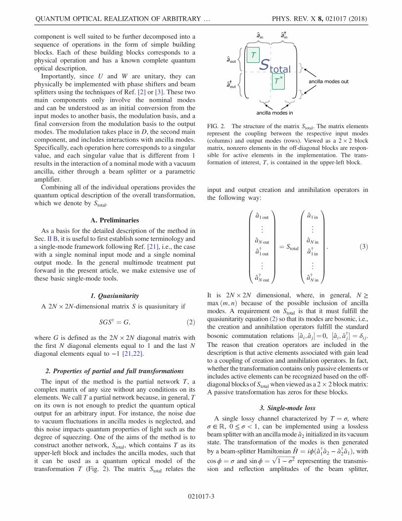
The input of the method is the partial network T, acomplex matrix of any size without any conditions on itselements. We call T a partial network because, in general, Ton its own is not enough to predict the quantum opticaloutput for an arbitrary input. For instance, the noise dueto vacuum fluctuations in ancilla modes is neglected, andthis noise impacts quantum properties of light such as thedegree of squeezing. One of the aims of the method is toconstruct another network, Stotal, which contains T as itsupper-left block and includes the ancilla modes, such thatit can be used as a quantum optical model of thetransformation T (Fig. 2). The matrix Stotal relates the

input and output creation and annihilation operators inthe following way:

0BBBBBBBBBBBB@

a1 out

..

.

aN out

a†1 out

..

.

a†N out

1CCCCCCCCCCCCA

¼ Stotal

0BBBBBBBBBBBB@

a1 in

..

.

aN in

a†1 in

..

.

a†N in

1CCCCCCCCCCCCA: ð3Þ

It is 2N × 2N dimensional, where, in general, N ≥max ðm; nÞ because of the possible inclusion of ancillamodes. A requirement on Stotal is that it must fulfill thequasiunitarity equation (2) so that its modes are bosonic, i.e.,the creation and annihilation operators fulfill the standardbosonic commutation relations ½ai; aj�¼0, ½ai; a†j � ¼ δij.The reason that creation operators are included in thedescription is that active elements associated with gain leadto a coupling of creation and annihilation operators. In fact,whether the transformation contains only passive elements orincludes active elements can be recognized based on the off-diagonal blocks of Stotal whenviewed as a 2 × 2 blockmatrix:A passive transformation has zeros for these blocks.

3. Single-mode loss

A single lossy channel characterized by T ¼ σ, whereσ ∈ R, 0 ≤ σ < 1, can be implemented using a losslessbeam splitter with an ancillamode a2 initialized in its vacuumstate. The transformation of the modes is then generatedby a beam-splitter Hamiltonian H ¼ iϕða†1a2 − a†2a1Þ, withcosϕ ¼ σ and sinϕ ¼

ffiffiffiffiffiffiffiffiffiffiffiffiffi1 − σ2

prepresenting the transmis-

sion and reflection amplitudes of the beam splitter,

FIG. 2. The structure of the matrix Stotal. The matrix elementsrepresent the coupling between the respective input modes(columns) and output modes (rows). Viewed as a 2 × 2 blockmatrix, nonzero elements in the off-diagonal blocks are respon-sible for active elements in the implementation. The trans-formation of interest, T, is contained in the upper-left block.

QUANTUM OPTICAL REALIZATION OF ARBITRARY … PHYS. REV. X 8, 021017 (2018)

021017-3

respectively. The connection between this Hamiltonian andthe corresponding transformation matrix

S ¼

0BBBBB@

σffiffiffiffiffiffiffiffiffiffiffiffiffi1 − σ2

p0 0

−ffiffiffiffiffiffiffiffiffiffiffiffiffi1 − σ2

pσ 0 0

0 0 σffiffiffiffiffiffiffiffiffiffiffiffiffi1 − σ2

p

0 0 −ffiffiffiffiffiffiffiffiffiffiffiffiffi1 − σ2

pσ

1CCCCCA;

ð4Þsuch that 0

BBBBB@

a1outa2outa†1outa†2out

1CCCCCA ¼ S

0BBBBB@

a1ina2ina†1ina†2in

1CCCCCA; ð5Þ

is described in Ref. [21], pp. 1215–1216 (see also [23]).

4. Single-mode gain

Similarly, for a single channel with gain given by T ¼ σ,where σ ∈ R, σ > 1, we introduce an ancilla mode a2,initially in vacuum. Gain can be realized with a parametricamplifier with a Hamiltonian H ¼ iξða†1a†2 − a1a2Þ, wherecosh ξ ¼ σ. The corresponding enlarged transformation

S ¼

0BBB@

σ 0 0ffiffiffiffiffiffiffiffiffiffiffiffiffiσ2 − 1

p

0 σffiffiffiffiffiffiffiffiffiffiffiffiffiσ2 − 1

p0

0ffiffiffiffiffiffiffiffiffiffiffiffiffiσ2 − 1

pσ 0ffiffiffiffiffiffiffiffiffiffiffiffiffi

σ2 − 1p

0 0 σ

1CCCA ð6Þ

can be constructed as described in Ref. [21], p. 1217.

5. Single-mode phase shift

Complex transformations involve phase shifts T ¼ eiφ

(φ ∈ R) for which no ancilla mode is required. TheHamiltonian is H ¼ −φa†1a1, and the transformation takesthe simple form of ða1 out

a†1 out

Þ ¼ Sða1 ina†1 inÞ, with

S ¼�eiφ 0

0 e−iφ

�: ð7Þ

B. Method

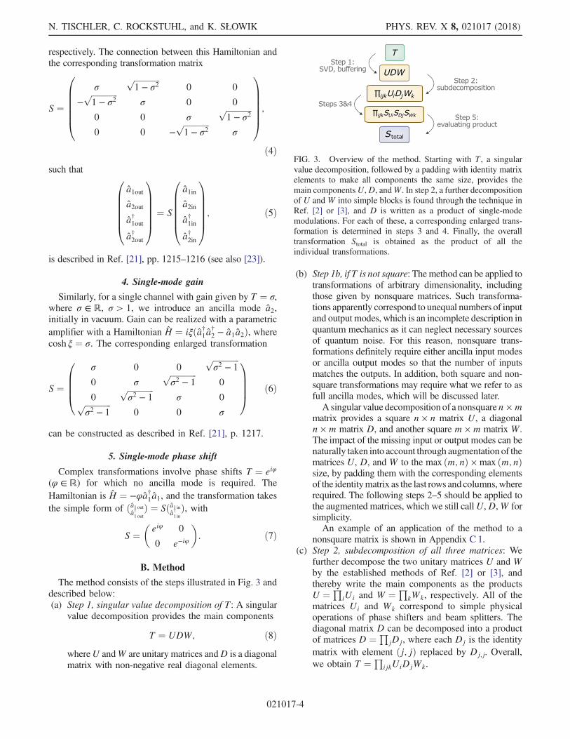
The method consists of the steps illustrated in Fig. 3 anddescribed below:(a) Step 1, singular value decomposition of T: A singular

value decomposition provides the main components

T ¼ UDW; ð8ÞwhereU andW are unitary matrices andD is a diagonalmatrix with non-negative real diagonal elements.

(b) Step 1b, if T is not square: The method can be applied totransformations of arbitrary dimensionality, includingthose given by nonsquare matrices. Such transforma-tions apparently correspond to unequal numbers of inputand output modes, which is an incomplete description inquantum mechanics as it can neglect necessary sourcesof quantum noise. For this reason, nonsquare trans-formations definitely require either ancilla input modesor ancilla output modes so that the number of inputsmatches the outputs. In addition, both square and non-square transformations may require what we refer to asfull ancilla modes, which will be discussed later.A singular value decomposition of a nonsquaren ×m

matrix provides a square n × n matrix U, a diagonaln ×m matrix D, and another square m ×m matrix W.The impact of the missing input or output modes can benaturally taken into account through augmentation of thematrices U, D, and W to the max ðm; nÞ × max ðm; nÞsize, by padding them with the corresponding elementsof the identitymatrix as the last rows andcolumns,whererequired. The following steps 2–5 should be applied tothe augmented matrices, which we still callU,D,W forsimplicity.An example of an application of the method to a

nonsquare matrix is shown in Appendix C 1.(c) Step 2, subdecomposition of all three matrices: We

further decompose the two unitary matrices U and Wby the established methods of Ref. [2] or [3], andthereby write the main components as the productsU ¼ Q

iUi and W ¼ QkWk, respectively. All of the

matrices Ui and Wk correspond to simple physicaloperations of phase shifters and beam splitters. Thediagonal matrix D can be decomposed into a productof matrices D ¼ Q

jDj, where each Dj is the identitymatrix with element ðj; jÞ replaced by Dj;j. Overall,we obtain T ¼ Q

ijkUiDjWk.

FIG. 3. Overview of the method. Starting with T, a singularvalue decomposition, followed by a padding with identity matrixelements to make all components the same size, provides themain componentsU,D, andW. In step 2, a further decompositionof U and W into simple blocks is found through the technique inRef. [2] or [3], and D is written as a product of single-modemodulations. For each of these, a corresponding enlarged trans-formation is determined in steps 3 and 4. Finally, the overalltransformation Stotal is obtained as the product of all theindividual transformations.

N. TISCHLER, C. ROCKSTUHL, and K. SŁOWIK PHYS. REV. X 8, 021017 (2018)

021017-4

(d) Step 3, determining the dimensionality of the enlargedsystem and assigning modes: The dimensionality ofthe enlarged matrices is 2N × 2N, with N given byN ≡ nN þ nA, where nN ≡max ðm; nÞ is the numberof nominal modes, i.e., the number of modes explicitlyincluded in T, and nA is the number of singular valuesof T not equal to 1. Modes 1 to nN are associated withthe nominal modes, while modes nN þ 1 to N areassociated with full ancilla modes, by which wedenote those modes that are added throughout thewhole transformation, not just as inputs or outputs tomatch the number of input and output modes, asdescribed in step 1b. Each nominal mode j has its owncorresponding ancilla mode mAj if the jth singularvalue of T differs from 1.

(e) Step 4, finding associated quasiunitary matrices: Weconstruct amatrixSUi for eachUi and, similarly, amatrixSWk for each Wk. Here, SUi and SWk are defined as

SUi ≡

0BBB@

Ui 0 0 0

0 InA 0 0

0 0 U�i 0

0 0 0 InA

1CCCA ð9Þ

and

SWk ≡

0BBB@

Wk 0 0 0

0 InA 0 0

0 0 W�k 0

0 0 0 InA

1CCCA; ð10Þ

respectively,withUi andWk being thenN × nN matricesfrom step 2, InA being the nA × nA identity matrix, andthe 0s being matrices of the appropriate size filled withzeros. In addition, we construct amatrixSDj for eachDj.For the special case in which the jth singular valueσj ¼ 1, SDj is the N × N identity matrix and thereforenot needed. Otherwise, if σj ≠ 1, the matrix SDj is theN × N identity matrix with the elements correspondingto the intersection of rows and columns j, mAj, jþ N,mAj þ N replaced by

0BBBBBBBB@

σjffiffiffiffiffiffiffiffiffiffiffiffiffi1 − σ2j

q0 0

−ffiffiffiffiffiffiffiffiffiffiffiffiffi1 − σ2j

qσj 0 0

0 0 σjffiffiffiffiffiffiffiffiffiffiffiffiffi1 − σ2j

q

0 0 −ffiffiffiffiffiffiffiffiffiffiffiffiffi1 − σ2j

qσj

1CCCCCCCCAð11Þ

if σj < 1, and

0BBBBBBBB@

σj 0 0ffiffiffiffiffiffiffiffiffiffiffiffiffiσ2j − 1

q

0 σjffiffiffiffiffiffiffiffiffiffiffiffiffiσ2j − 1

q0

0ffiffiffiffiffiffiffiffiffiffiffiffiffiσ2j − 1

qσj 0ffiffiffiffiffiffiffiffiffiffiffiffiffi

σ2j − 1q

0 0 σj

1CCCCCCCCA

ð12Þ

ifσj > 1.This alsoallowsus todealwith transformationsthat combine loss in some modes with gain in others,which previously proposed methods did not accommo-date. An example can be found in Appendix B 2.

(f) Step 5, multiplication of quasiunitary matrices toobtain the overall transformation: We obtain theoverall enlarged transformation as

Stotal ¼Yijk

SUiSDjSWk: ð13Þ

A proof that Stotal fulfills the quasiunitarity equation (2)and contains T as its upper-left block can be found inAppendix A, and an example decomposition is shownin Appendix B 1.

(g) Implementation of the decomposition in terms ofsimple building blocks: The full decompositionStotal ¼

QijkSUiSDjSWk provides a recipe for an im-

plementation in terms of the simple building blocks ofphase shifters, beam splitters, and parametric ampli-fiers, as each of the matrices in the decompositiondirectly corresponds to such a building block. Thefactors SUi and SWk correspond to beam splitters andphase shifters involving the nominal modes, i.e., thefirst nN modes. The factors SDj that differ from theidentity correspond to beam splitters and parametricamplifiers, each involving one of the nominal modesand one of the full ancilla modes.

III. DISCUSSION

Section II has shown how a full enlarged quantumoptical network can be mathematically represented andphysically realized. Now, we are also in a position toanswer the remaining questions from the Introduction.Contrary to conclusions of earlier works devoted to setupswith either loss or gain alone, any transformation isavailable. The decomposition works for all linear networksas an input since a singular value decomposition can beperformed for any complex matrix. This means that, inprinciple, any transformation can be realized, even if thepractical implementation of arbitrary two-mode squeezingis technically challenging [24].The number of required ancilla modes is tied to the

dimensionality of T if it is not square, as well as to its

QUANTUM OPTICAL REALIZATION OF ARBITRARY … PHYS. REV. X 8, 021017 (2018)

021017-5

singular values. A nonsquare n ×m transformation T leadsto (m − n) output ancilla modes if m > n, or to (n −m)input ancilla modes if n > m. In addition to these input oroutput ancilla modes, full ancilla modes are introduced, andtheir number is equal to the number of singular values of Tthat are not equal to 1. Each singular value below (above) 1entails a beam-splitter operation (parametric amplification)with such an ancilla mode. For the special case in which Tis square and all of its singular values are equal to 1, noancilla modes are needed because T is unitary, and thenthe method can be reduced to the known unitary decom-positions (Ref. [2] or [3]). Upper bounds on the numberof elemental building blocks required when using thescheme depend on the dimensionality of T in the followingway: The maximum number of variable beam splittersneeded to implement the unitary blocks U and W isnðn − 1Þ=2þmðm − 1Þ=2, while the maximum numberof phase shifters is nðnþ1Þ=2þmðmþ1Þ=2. Additionally,up to minðm; nÞ elements are required to implementD; theseelements are either beam splitters or parametric amplifiers.Hence, the number of parametric amplifiers only scaleslinearly with the size of the transformation matrix.A unitary network followed by photon detection in the

different modes can be used to implement a projectivemeasurement in a Hilbert space with a dimensionalitymatching the unitary network. In the context of generalizedmeasurements, it is possible for a POVM to have a numberof measurement outcomes that is larger than the dimen-sionality of the system. The Naimark dilation theoremguarantees that such a POVM can be implemented as aprojective measurement in an enlarged Hilbert space [25].Our method can be used to find a Naimark extension, whichprovides a suitable enlarged unitary transformation for thisprojective measurement (see Appendix C 1).Another possible application of the method lies in the

construction of probabilistic optical quantum informationprotocols. Starting with a general transformation matrix, byformulating the action of the protocol as a mapping from agiven set of input states to a set of desired output states, asystem of possibly nonlinear equations for the elements ofT can be constructed. A solution of the system of equationsdefines a network that performs the protocol, and themethod can then be used to find an implementation of thatnetwork (for an example, see Appendix C 2).Although the decomposition always provides a full

quantum optical transformation with the dependence ofthe mean output fields on the mean input fields as specifiedby the partial network T, the implementation is not unique.This is already evident from the simplest nonunitary“network,” a single channel with loss or gain. As discussedin Ref. [21], the same mean field could be achieved byincluding excess gain and loss that compensate each other’seffect on the mean field, at the expense of a reduction in thepurity of the state. Given that this leaves the first moment ofthe field invariant but changes higher-order moments, it

presents an opportunity to tailor the higher-order moments.It is an interesting question (beyond the scope of the presentarticle) whether the multimode control over first momentsof the field provided by the method could be extended tohigher-order moments.

IV. CONCLUSION

In summary, we have presented a way to describe andimplement an arbitrary linear optical transformation,which can have any size and does not need to be completein the sense that its modes fulfill bosonic commutationrelations. This is achieved by finding a transformation inan enlarged space that includes the network of interest.The ancilla modes included in the description enablerigorous quantum optical modeling of the gains and lossesin the network. In addition, a decomposition into the basicbuilding blocks of beam splitters, phase shifters, andparametric amplifiers is obtained. This shows a way toimplement the network that could physically be realizedwith integrated optics. We have discussed the role that thesingular values of the transformation matrix play withrespect to the number and type of ancilla modes. Themethod could prove useful for the implementation ofPOVMs, the design of probabilistic optical quantuminformation protocols, and, more generally, in any appli-cation that involves nonunitary networks.We provide a MATLAB code for numerically imple-

menting the full decomposition on GitHub [34].

ACKNOWLEDGMENTS

We wish to acknowledge discussions with AntonZeilinger, Gabriel Molina-Terriza, Geoff Pryde, TimRalph, Howard Wiseman, Michael Hall, and StephenBarnett and his group. Part of this work was supportedby Australian Research Council Grant No. DP160101911,the Austrian Academy of Sciences (ÖAW), and the AustrianScience Fund (FWF) with SFB F40 (FOQUS). K. S.acknowledges support from the Foundation for PolishScience (Project HEIMaT No. Homing/2016-1/8) withinthe European Regional Development Fund. C. R. and K. S.also wish to thank the Deutscher AkademischerAustauschdienst (PPP Poland) and the Ministry ofScience and Higher Education in Poland for support.

APPENDIX A: PROOF THAT THE PRODUCTStotal =

QijkSUiSDjSWk RESULTS IN A

QUASIUNITARY MATRIX WITH T AS ITSUPPER-LEFT BLOCK

First, it should be noted that the individual S matrices(SUi, SDj, and SWk) fulfill Eq. (2). The product of twomatrices that fulfill Eq. (2) is another quasiunitary matrix,which can be seen as follows.

N. TISCHLER, C. ROCKSTUHL, and K. SŁOWIK PHYS. REV. X 8, 021017 (2018)

021017-6

Let A and B fulfill Eq. (2). Then,

M ¼ AB;

MGM† ¼ ðABÞGðABÞ† ¼ AðBGB†ÞA† ¼ AGA† ¼ G:

Therefore, Stotal is quasiunitary.The second part of the proof is that the product of the

individual S matrices has T as its upper-left block.We have T ¼ UDW ¼ Q

ijkUiDjWk, and Stotal ¼QijkSUiSDjSWk. Because of the block structure of the

matrices SUi and SWk,

Yi

SUi ¼

0BBBBBB@

QiUi 0 0 0

0 InA 0 0

0 0Qi0U�

i0 0

0 0 0 InA

1CCCCCCA;

and similarly,

Yk

SWk ¼

0BBBBBB@

QkWk 0 0 0

0 InA 0 0

0 0Qk0W�

k0 0

0 0 0 InA

1CCCCCCA:

The components SDj corresponding to Dj generally donot have the same structure. The matrix SDj is the identitymatrix if the jth singular value of T, σj ¼ 1. Otherwise, ifσj ≠ 1, j and mAj are the mode numbers corresponding tothe nominal mode and ancilla mode, respectively, of the jthsingular value. Then, each matrix SDj is the identity matrixwith the elements corresponding to the intersection of rowsand columns j, mAj, jþ N, mAj þ N replaced as given byexpressions (11) and (12).The fact that Stotal ¼

QijkSUiSDjSWk has T ¼Q

ijkUiDjWk as its upper-left block can be shown byobserving the structure of the matrix as the multiplication iscarried out. Let us consider the multiplication by startingfrom the rightmost matrix, sequentially multiplying fromthe left by the other matrices as specified, and denoting theproduct after x steps as Sx. The rows of Sx that deviate fromthose of the identity matrix are of interest at different stagesof the multiplication, i.e., for different x. Let x1 equal thenumber of matrices in the decomposition of W. ForSx1 ¼

QkSWk, we have already seen that the upper-left

block of Sx1 is the product of the upper-left blocks of thecomponents and that the only elements that deviate from

the identity matrix are contained in the blocksð1∶nN; 1∶nNÞ and ð1þ N∶nN þ N; 1þ N∶nN þ NÞ [26].Now, as each SDj is multiplied from the left, there areat most two new rows of the resulting matrix thatcan deviate from the identity: rows mAj and ðmAj þ NÞwhen σj ≠ 1. Let x2 lie between x1 and the number ofmatrices in the decomposition of DW. After each step,the upper-left block of Sx2 is the product of the upper-left blocks of the components because the elementsðmAj; 1∶nNÞ and ðmAj þ N; 1∶nNÞ of Sx2−1 are zero.This is essentially due to the fact that a unique ancillamode is assigned to each singular value that is differentfrom 1. After having multiplied through the individual Smatrices corresponding to DW, for

QiSUi we again have

the block structure that guarantees that the upper-left blockof Stotal is T.

APPENDIX B: EXAMPLES

We demonstrate the method using two examples. First,we discuss how the lossy beam splitter with apparentnonlinearity can be constructed with standard opticalelements. We then apply the method to an arbitrary 2×2transformation, which may combine loss and gain indifferent modes, to obtain an analytic decomposition.

1. Lossy beam splitter with apparentnonlinear action

Here, the method is applied to decompose the 2 × 2

transformation T ¼ 12ð 1−1

−11Þ into simple building blocks.

We begin with a singular value decomposition ofT¼UDW, which gives U¼ð1= ffiffiffi

2p Þð−1

111Þ, D¼ð1

000Þ,

and W ¼ ð1= ffiffiffi2

p Þð−1−1 1−1Þ. Since T is square, no augmenta-

tion of U, D, or W is required. Further decomposition

provides U ¼ ð−10

01Þ� 1ffiffi

2p1ffiffi2

p− 1ffiffi

2p1ffiffi2

p

�, while W is already a beam

splitter, one of the basic building blocks. The matrix Ddoes not need to be decomposed further because of its simpleform: The diagonal element 0 in D represents a completeattenuation of amode and constitutes the only singular valuedifferent from 1. One can thus proceed to identify thenumber of ancilla modes nA ¼ 1, so that N ¼ 3 and thedimensionality of the corresponding S matrix is 6 × 6,

0BBBBBBBBBB@

a1outa2outa3out

a†1outa†2outa†3out

1CCCCCCCCCCA

¼ S

0BBBBBBBBBB@

a1ina2ina3in

a†1ina†2ina†3in

1CCCCCCCCCCA;

with the nominal modes a1 and a2, and the ancilla mode a3.

QUANTUM OPTICAL REALIZATION OF ARBITRARY … PHYS. REV. X 8, 021017 (2018)

021017-7

We continue to identify the SU, SD, and SW matricescorresponding to individual operations based onEqs. (9)–(11):

Y2i¼1

SUi ¼

0BBBBBBBBB@

−1 0 0 0 0 0

0 1 0 0 0 0

0 0 1 0 0 0

0 0 0 −1 0 0

0 0 0 0 1 0

0 0 0 0 0 1

1CCCCCCCCCA

×

0BBBBBBBBBB@

1ffiffi2

p −1ffiffi2

p 0 0 0 0

1ffiffi2

p 1ffiffi2

p 0 0 0 0

0 0 1 0 0 0

0 0 0 1ffiffi2

p −1ffiffi2

p 0

0 0 0 1ffiffi2

p 1ffiffi2

p 0

0 0 0 0 0 1

1CCCCCCCCCCA;

SW ¼

0BBBBBBBBBB@

−1ffiffi2

p 1ffiffi2

p 0 0 0 0

−1ffiffi2

p −1ffiffi2

p 0 0 0 0

0 0 1 0 0 0

0 0 0 −1ffiffi2

p 1ffiffi2

p 0

0 0 0 −1ffiffi2

p −1ffiffi2

p 0

0 0 0 0 0 1

1CCCCCCCCCCA;

SD ¼

0BBBBBBBBB@

1 0 0 0 0 0

0 0 1 0 0 0

0 −1 0 0 0 0

0 0 0 1 0 0

0 0 0 0 0 1

0 0 0 0 −1 0

1CCCCCCCCCA:

The total transformation matrix

Stotal ¼Yi

SUiSDSW ¼

0BBBBBBBBBBBB@

12

−12

1ffiffi2

p 0 0 0

−12

12

1ffiffi2

p 0 0 0

1ffiffi2

p 1ffiffi2

p 0 0 0 0

0 0 0 12

−12

1ffiffi2

p

0 0 0 −12

12

1ffiffi2

p

0 0 0 1ffiffi2

p 1ffiffi2

p 0

1CCCCCCCCCCCCA

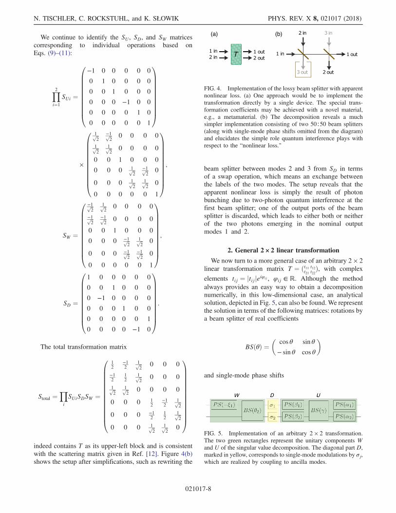
indeed contains T as its upper-left block and is consistentwith the scattering matrix given in Ref. [12]. Figure 4(b)shows the setup after simplifications, such as rewriting the

beam splitter between modes 2 and 3 from SD in termsof a swap operation, which means an exchange betweenthe labels of the two modes. The setup reveals that theapparent nonlinear loss is simply the result of photonbunching due to two-photon quantum interference at thefirst beam splitter; one of the output ports of the beamsplitter is discarded, which leads to either both or neitherof the two photons emerging in the nominal outputmodes 1 and 2.

2. General 2 × 2 linear transformation

We now turn to a more general case of an arbitrary 2 × 2

linear transformation matrix T ¼ ðt11t21t12t22Þ, with complex

elements tij ¼ jtijjeiφij , φij ∈ R. Although the methodalways provides an easy way to obtain a decompositionnumerically, in this low-dimensional case, an analyticalsolution, depicted in Fig. 5, can also be found. We representthe solution in terms of the following matrices: rotations bya beam splitter of real coefficients

BSðθÞ ¼�

cos θ sin θ

− sin θ cos θ

�

and single-mode phase shifts

(a) (b)

FIG. 4. Implementation of the lossy beam splitter with apparentnonlinear loss. (a) One approach would be to implement thetransformation directly by a single device. The special trans-formation coefficients may be achieved with a novel material,e.g., a metamaterial. (b) The decomposition reveals a muchsimpler implementation consisting of two 50∶50 beam splitters(along with single-mode phase shifts omitted from the diagram)and elucidates the simple role quantum interference plays withrespect to the “nonlinear loss."

FIG. 5. Implementation of an arbitrary 2 × 2 transformation.The two green rectangles represent the unitary components Wand U of the singular value decomposition. The diagonal part D,marked in yellow, corresponds to single-mode modulations by σj,which are realized by coupling to ancilla modes.

N. TISCHLER, C. ROCKSTUHL, and K. SŁOWIK PHYS. REV. X 8, 021017 (2018)

021017-8

PS1ðθÞ ¼�eiθ 0

0 1

�; PS2ðθÞ ¼

�1 0

0 eiθ

�:

To solve this case analytically, one can transform the Tmatrix to a real form Tre through the following sequence ofoperations:(1) Cancel phases in the left column

T → T1 ¼ PS1ð−φ11Þ:PS2ð−φ21Þ:T

¼� jt11j jt12jeiðφ12−φ11Þ

jt21j jt22jeiðφ22−φ21Þ

�;

where matrix multiplication is indicated by “.” forclarity.

(2) Rotate the matrix to make the bottom-left compo-nent zero

T1 → T2 ¼ BSðϑÞ:T1 ¼�t11 t120 t22

�;

where ϑ ¼ arctan ½ðjt21jÞ=ðjt11jÞ� and

t11 ¼ jt11j cos ϑþ jt21j sin ϑ;t12 ¼ jt12j cos ϑeiðφ12−φ11Þ þ jt22j sin ϑeiðφ22−φ21Þ;

t22 ¼ −jt12j sin ϑeiðφ12−φ11Þ þ jt22j cos ϑeiðφ22−φ21Þ:

Note that t11 is real and non-negative, which weemphasize below by explicitly writing t11 ¼ jt11j.

(3) Cancel phases in the right column,

T2 → T3 ¼ PS1ð−ξ1Þ:PS2ð−ξ2Þ:T2

¼� jt11je−iξ1 jt12j

0 jt22j

�;

with ξj ¼ arg tj2.(4) Cancel the remaining phase in the left column,

T3 → Tre ¼ T3:PS1ðξ1Þ ¼� jt11j jt12j

0 jt22j

�:

Finally, the transformed real matrix reads

Tre ¼ PS1ð−ξ1Þ:PS2ð−ξ2Þ:BSðϑÞ× PS1ð−φ11Þ:PS2ð−φ21Þ:T:PS1ðξ1Þ: ðB1Þ

A singular value decomposition of the resulting real 2 × 2matrix is especially simple, with the unitary componentsgiven as two beam-splitter rotations. In this particular case,we make use of the fact that one of the components is 0 andobtain

Tre ¼ BSðθ1Þ:D:BSðθ2Þ; ðB2Þ

where

θj ¼ð−1Þj2

arg ðqj þ 2pjiÞ;pj ¼ jt1;3−jt3−j;2j;qj ¼ jt11j2 − jt22j2 þ ð−1Þj−1jt12j2:

The matrix of singular values determines the requireddegree of attenuation or amplification,

D ¼�σ1 0

0 σ2

�;

σj ¼

ffiffiffiffiffiffiffiffiffiffiffiffiffiffiffiffiffiffiffiffiffiffiffiffiffiffiffiffiffiffiffiffiffiffiffiffiffiffiffiffiffiffiffiffiffiffisþ ð−1Þj−1

ffiffiffiffiffiffiffiffiffiffiffiffiffiffiffiffiffiffiq2j þ 4p2

j

q2

vuut;

s ¼ jt11j2 þ jt22j2 þ jt12j2:

Finally, a combination of Eqs. (B1) and (B2) yields thedecomposition of the original matrix T,

T ¼ PS2ðφ21Þ:PS1ðφ11Þ:BSð−ϑÞ:PS2ðξ2Þ:PS1ðξ1Þ:BSðθ1Þ|fflfflfflfflfflfflfflfflfflfflfflfflfflfflfflfflfflfflfflfflfflfflfflfflfflfflfflfflfflfflfflfflfflfflfflfflfflfflfflfflfflfflfflfflfflfflffl{zfflfflfflfflfflfflfflfflfflfflfflfflfflfflfflfflfflfflfflfflfflfflfflfflfflfflfflfflfflfflfflfflfflfflfflfflfflfflfflfflfflfflfflfflfflfflffl}U

×D:BSðθ2Þ:PS1ð−ξ1Þ|fflfflfflfflfflfflfflfflfflfflfflfflffl{zfflfflfflfflfflfflfflfflfflfflfflfflffl}W

:

Note that the matrix U can be further simplified to

U ¼ PS1

0B@φ11 þ ξ1 þ

αþ β

2|fflfflfflfflfflfflfflfflfflfflfflfflffl{zfflfflfflfflfflfflfflfflfflfflfflfflffl}α1

1CA:PS2

0B@φ21 þ ξ2 −

αþ β

2|fflfflfflfflfflfflfflfflfflfflfflfflffl{zfflfflfflfflfflfflfflfflfflfflfflfflffl}α2

1CA

× BSðγÞ:PS1

0B@α − β

2|ffl{zffl}β1

1CA:PS2

0B@β − α

2|ffl{zffl}β2

1CA;

α ¼ arg ðcosϑ cos θ1 þ sinϑ sin θ1eiðξ2−ξ1ÞÞ;β ¼ arg ðcosϑ sin θ1 − sinϑ cos θ1eiðξ2−ξ1ÞÞ;γ ¼ arccos ðj cos ϑ cos θ1 þ sinϑ sin θ1eiðξ2−ξ1ÞjÞ:

The construction of the S network depends on the singularvalues σ1;2 and can be obtained from Eqs. (9)–(12). Thedimensionality of S is at most 8 × 8 since there is one ancillamode per singular value that is not equal to 1. For a particularexample, the case of a transformation combining lossin mode 1 (σ1 < 1) with gain in mode 2 (σ2 > 1), thesubmatrices read

QUANTUM OPTICAL REALIZATION OF ARBITRARY … PHYS. REV. X 8, 021017 (2018)

021017-9

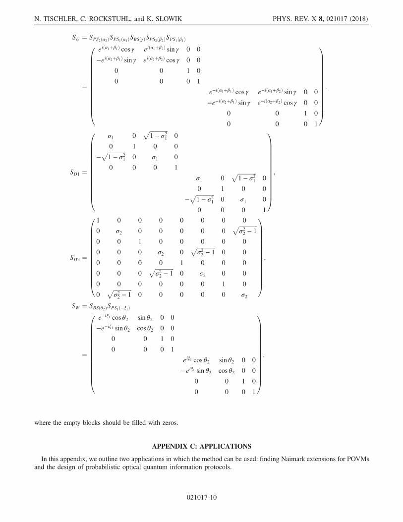
SU ¼ SPS2ðα2ÞSPS1ðα1ÞSBSðγÞSPS2ðβ2ÞSPS1ðβ1Þ

¼

0BBBBBBBBBBBBB@

eiðα1þβ1Þ cos γ eiðα1þβ2Þ sin γ 0 0

−eiðα2þβ1Þ sin γ eiðα2þβ2Þ cos γ 0 0

0 0 1 0

0 0 0 1

e−iðα1þβ1Þ cos γ e−iðα1þβ2Þ sin γ 0 0

−e−iðα2þβ1Þ sin γ e−iðα2þβ2Þ cos γ 0 0

0 0 1 0

0 0 0 1

1CCCCCCCCCCCCCA

;

SD1 ¼

0BBBBBBBBBBBBB@

σ1 0ffiffiffiffiffiffiffiffiffiffiffiffiffi1 − σ21

p0

0 1 0 0

−ffiffiffiffiffiffiffiffiffiffiffiffiffi1 − σ21

p0 σ1 0

0 0 0 1

σ1 0ffiffiffiffiffiffiffiffiffiffiffiffiffi1 − σ21

p0

0 1 0 0

−ffiffiffiffiffiffiffiffiffiffiffiffiffi1 − σ21

p0 σ1 0

0 0 0 1

1CCCCCCCCCCCCCA

;

SD2 ¼

0BBBBBBBBBBBBB@

1 0 0 0 0 0 0 0

0 σ2 0 0 0 0 0ffiffiffiffiffiffiffiffiffiffiffiffiffiσ22 − 1

p0 0 1 0 0 0 0 0

0 0 0 σ2 0ffiffiffiffiffiffiffiffiffiffiffiffiffiσ22 − 1

p0 0

0 0 0 0 1 0 0 0

0 0 0ffiffiffiffiffiffiffiffiffiffiffiffiffiσ22 − 1

p0 σ2 0 0

0 0 0 0 0 0 1 0

0ffiffiffiffiffiffiffiffiffiffiffiffiffiσ22 − 1

p0 0 0 0 0 σ2

1CCCCCCCCCCCCCA

;

SW ¼ SBSðθ2ÞSPS1ð−ξ1Þ

¼

0BBBBBBBBBBBBB@

e−iξ1 cos θ2 sin θ2 0 0

−e−iξ1 sin θ2 cos θ2 0 0

0 0 1 0

0 0 0 1

eiξ1 cos θ2 sin θ2 0 0

−eiξ1 sin θ2 cos θ2 0 0

0 0 1 0

0 0 0 1

1CCCCCCCCCCCCCA

;

where the empty blocks should be filled with zeros.

APPENDIX C: APPLICATIONS

In this appendix, we outline two applications in which the method can be used: finding Naimark extensions for POVMsand the design of probabilistic optical quantum information protocols.

N. TISCHLER, C. ROCKSTUHL, and K. SŁOWIK PHYS. REV. X 8, 021017 (2018)

021017-10

1. POVMs

A POVM is determined by a set of positive semidefiniteoperators fEigmi¼1, which sum to identity

Pmi¼1 Ei ¼ In and

represent generalized measurements in an n-dimensionalHilbert space [27]. Here, In denotes the n-dimensionalidentity matrix. An active field of research has been focusedon the physical implementation of POVMs [28–32]. One ofthe strategies is based on Naimark’s dilation theorem.According to the theorem, any POVM can be realized asa projective measurement in an enlarged Hilbert spaceH [25]. However, the theorem does not itself provide ageneral recipe to find the extension to H, called Naimarkextension.To see how our method can be exploited to find Naimark

extensions, let us focus on the important case of rank-onePOVMs. The operators forming rank-one POVMs corre-spond to projectors Ei ¼ jϕðiÞihϕðiÞj on, in general, non-orthogonal vectors jϕðiÞi in the original Hilbert space. ANaimark extension can be found by augmenting the vectorsjϕðiÞi to sizem so that they become orthogonal inH. For thispurpose, let us define a rectangular n ×m matrix withcolumns given by the n-dimensional vectors jϕðiÞi:

T ¼

0BB@

ϕð1Þ1 … ϕðmÞ

1

..

. ...

ϕð1Þn … ϕðmÞ

n

1CCA;

such that TT† ¼ I. Here, ϕðiÞj stand for elements of jϕðiÞi. A

singular value decomposition of T ¼ UDW provides aunitary n × n matrix U, an n ×m matrix D, and a unitarym ×m matrix W. Note that since TT† ¼ I, all the singularvalues of T are equal to 1. This means that the dimension-ality of the Naimark extension found with this method is m,and the number of ancilla output modes is m − n. Next, letus pad the matrices of smaller dimensionalities with ele-ments of the identity matrix, in accordance with step 1b ofthe method. As a result, we obtain the enlarged m ×mmatrices:

U →

�U 0

0 Im−n

�; D → Im;

and W does not require any modification. The productUDW ¼ UW is unitary and becomes an m-dimensionalNaimark extension of T, which can be directly decomposedinto building blocks with the methods of Reck et al. [2] orClements et al. [3]. This procedure allows us to design anetwork for an arbitrary rank-one POVM.

2. Design of probabilistic protocols

Here, we demonstrate how the method can be used in thedesign of probabilistic optical quantum logic gates. We

illustrate the design on the example of a two-qubit con-trolled-Z gate and show a systematic way to find the setuppresented in Ref. [33]. A two-qubit controlled-Z gate canbe implemented with two photons and four optical modes.The control qubit is encoded by one photon within the firsttwo modes (called the control modes), while the targetqubit is encoded by another photon in the last two modes(the target modes). The goal is to construct a transformationusing passive optical elements, such that it implements acontrolled phase flip, given that both the input and outputstates fulfill the condition that there is one photon in thecontrol modes and one photon in the target modes.Our starting point is the desired effect on two-photon

states: For the four different input states below and onlyconsidering outputs according to the postselection con-dition of having one photon in a control mode and the otherphoton in a target mode, we want the circuit to output thefollowing states:

acHinatHin → −kacHoutatHout;

acHinatVin → kacHoutatVout;

acVinatHin → kacVoutatHout;

acVinatVin → kacVoutatVout; ðC1Þ

where the four modes are denoted cH, cV, tH, tV, afterhorizontal and vertical polarization in the control and targetmodes. The real constant k ∈ ð0; 1� allows for the possibilityof the protocol being probabilistic, with a success rate of k2.The above transformations involve four input and outputmodes, so the transformation we seek has the general form

T ¼

0BBB@

t11 t12 t13 t14t21 t22 t23 t24t31 t32 t33 t34t41 t42 t43 t44

1CCCA:

Since we assume that the setup will be passive, we know thatStotal will be block diagonal and can be written as

Stotal ¼�A 0

0 A�

�;

where A is a unitary matrix that contains T as its upper-leftblock, relating annihilation operators as follows:

0BBBBBBBB@

acHout

acVoutatHout

atVout

..

.

1CCCCCCCCA

¼�

T A12

A21 A22

�0BBBBBBBB@

acHin

acVinatHin

atVin

..

.

1CCCCCCCCA:

QUANTUM OPTICAL REALIZATION OF ARBITRARY … PHYS. REV. X 8, 021017 (2018)

021017-11

Based on the constraints of Eq. (C1), the elements of Tneed to be determined. To do this, it is useful to write theannihilation operators of the input modes in terms of thoseof the output modes. The unitary matrix A can simply beinverted to write the input modes in terms of the outputmodes, and we obtain

0BBBBBBBB@

acHin

acVinatHin

atVin

..

.

1CCCCCCCCA

¼�

T† A†21

A†12 A†

22

�0BBBBBBBB@

acHout

acVoutatHout

atVout

..

.

1CCCCCCCCA: ðC2Þ

Using Eq. (C1) together with Eq. (C2), we obtain a set ofnonlinear equations, of which one solution is

T ¼

0BBBBB@

t11 0 t13 0

0 t11 0 0

t31 0 − t13t312t11

0

0 0 0 − t13t312t11

1CCCCCA; k ¼ −

1

2t13t31:

There are three free parameters, t11, t13, t31, and the successprobability of the protocol, k2, depends on two of theseparameters. Moreover, the singular values of T depend onthe parameters. We need all the singular values to be lessthan or equal to 1 so that the circuit is a passive network, butwe would like as many of the values as possible to be 1 sothat the number of ancilla modes is minimized. A suitable

choice of parameters is t11 ¼ffiffi13

q, t13 ¼ t31 ¼

ffiffi23

q. This

choice results in the success probability of the protocol

k2 ¼ 19and the singular values ð1; 1;

ffiffi13

q;

ffiffi13

qÞ, which show

that two ancilla modes are required. From here, thedecomposition method can be used to find the physicalrealization of the matrix

T ¼

0BBBBBBBBB@

ffiffi13

q0

ffiffi23

q0

0ffiffi13

q0 0ffiffi

23

q0 −

ffiffi13

q0

0 0 0 −ffiffi13

q

1CCCCCCCCCA;

which finally provides the scheme of Ref. [33].

[1] By the terms “linear transformation” and “linear network”we refer to transformations for which the expectation valuesof the fields are related by a linear transformation between

the input and output modes and the annihilation operators ofthe output modes have the same linear dependence on theinput annihilation operators.

[2] M. Reck, A. Zeilinger, H. J. Bernstein, and P. Bertani,Experimental Realization of Any Discrete Unitary Oper-ator, Phys. Rev. Lett. 73, 58 (1994).

[3] W. R. Clements, P. C. Humphreys, B. J. Metcalf, W. S.Kolthammer, and I. A. Walsmley, Optimal Design forUniversal Multiport Interferometers, Optica 3, 1460 (2016).

[4] S. M. Barnett, J. Jeffers, A. Gatti, and R. Loudon, QuantumOptics of Lossy Beam Splitters, Phys. Rev. A 57, 2134(1998).

[5] L. Knöll, S. Scheel, E. Schmidt, D.-G. Welsch, and A. V.Chizhov, Quantum-State Transformation by Dispersive andAbsorbing Four-Port Devices, Phys. Rev. A 59, 4716(1999).

[6] J. Jeffers, Interference and the Lossless Lossy Beam Splitter,J. Mod. Opt. 47, 1819 (2000).

[7] S. Scheel, L. Knöll, T. Opatrný, and D.-G. Welsch,Entanglement Transformation at Absorbing and AmplifyingFour-Port Devices, Phys. Rev. A 62, 043803 (2000).

[8] C. Lee, M. Tame, J. Lim, and J. Lee, Quantum Plasmonicswith a Metal Nanoparticle Array, Phys. Rev. A 85, 063823(2012).

[9] D. A. B. Miller, Self-Configuring Universal Linear OpticalComponent, Photonics Res. 1, 1 (2013).

[10] D. A. B. Miller, All Linear Optical Devices Are ModeConverters, Opt. Express 20, 23985 (2012).

[11] S. Dutta Gupta and G. S. Agarwal, Two-Photon QuantumInterference in Plasmonics: Theory and Applications, Opt.Lett. 39, 390 (2014).

[12] T. Roger, S. Vezzoli, E. Bolduc, J. Valente, J. J. F. Heitz, J.Jeffers, C. Soci, J. Leach, C. Couteau, N. I. Zheludev, and D.Faccio, Coherent Perfect Absorption in Deeply Subwave-length Films in the Single-Photon Regime, Nat. Commun. 6,7031 (2015).

[13] T. Roger, S. Restuccia, A. Lyons, D. Giovannini, J. Romero,J. Jeffers, M. Padgett, and D. Faccio, Coherent Absorptionof N00N States, Phys. Rev. Lett. 117, 023601 (2016).

[14] R. Uppu, T. A. W. Wolterink, T. B. H. Tentrup, and P.W. H.Pinkse, Quantum Optics of Lossy Asymmetric Beam Split-ters, Opt. Express 24, 16440 (2016).

[15] G. Di Martino, Y. Sonnefraud, M. S. Tame, S. Kena-Cohen,F. Dieleman, Ş. K. Özdemir, M. S. Kim, and S. A. Maier,Observation of Quantum Interference in the PlasmonicHong-Ou-Mandel Effect, Phys. Rev. Applied 1, 034004(2014).

[16] Y.-J. Cai, M. Li, X.-F. Ren, C.-L. Zou, X. Xiong, H.-L.Lei, B.-H. Liu, G.-P. Guo, and G.-C. Guo, High-VisibilityOn-Chip Quantum Interference of Single Surface Plasmons,Phys. Rev. Applied 2, 014004 (2014).

[17] G. Fujii, D. Fukuda, and S. Inoue, Direct Observation ofBosonic Quantum Interference of Surface Plasmon Polar-itons Using Photon-Number-Resolving Detectors, Phys.Rev. B 90, 085430 (2014).

[18] J. S. Fakonas, A. Mitskovets, and H. A. Atwater, PathEntanglement of Surface Plasmons, New J. Phys. 17,023002 (2015).

[19] P. van Loock, Optical Hybrid Approaches to QuantumInformation, Laser Photonics Rev. 5, 167 (2011).

N. TISCHLER, C. ROCKSTUHL, and K. SŁOWIK PHYS. REV. X 8, 021017 (2018)

021017-12

[20] B. He, J. A. Bergou, and Z. Wang, Implementation ofQuantum Operations on Single-Photon Qudits, Phys. Rev.A 76, 042326 (2007).

[21] U. Leonhardt, Quantum Physics of Simple Optical Instru-ments, Rep. Prog. Phys. 66, 1207 (2003).

[22] J. Williamson, Quasi-unitary Matrices, Duke Math. J. 3,715 (1937).

[23] We use a slightly different definition for the matrix H in thisconnection: H ¼ iG ln S.

[24] U. L. Andersen, T. Gehring, C. Marquardt, and G. Leuchs,30 Years of Squeezed Light Generation, Phys. Scr. 91,053001 (2016).

[25] A. Peres, Neumark’s Theorem and Quantum Inseparability,Found. Phys. 20, 1441 (1990).

[26] By ða∶b; c∶dÞ, we denote the submatrix consisting of theintersection of rows a to b and columns c to d of the originalmatrix.

[27] M. Nielsen and I. Chuang, Quantum Computationand Quantum Information (Cambridge University Press,Cambridge, England, 2000).

[28] B. He and J. A. Bergou, A General Approach to PhysicalRealization of Unambiguous Quantum-State Discrimina-tion, Phys. Lett. A 356, 306 (2006).

[29] G. N. M. Tabia, Experimental Scheme for Qubit and QutritSymmetric Informationally Complete Positive Operator-Valued Measurements Using Multiport Devices, Phys.Rev. A 86, 062107 (2012).

[30] Z. Bian, J. Li, H. Qin, X. Zhan, R. Zhang, B. C. Sanders,and P. Xue, Realization of Single-Qubit Positive-Operator-Valued Measurement via a One-Dimensional PhotonicQuantum Walk, Phys. Rev. Lett. 114, 203602 (2015).

[31] N. Bent, H. Qassim, A. A. Tahir, D. Sych, G. Leuchs,L. L. Sánchez-Soto, E. Karimi, and R. W. Boyd, Exper-imental Realization of Quantum Tomography of PhotonicQudits via Symmetric Informationally Complete PositiveOperator-Valued Measures, Phys. Rev. X 5, 041006(2015).

[32] H. Sosa-Martinez, N. K. Lysne, C. H. Baldwin, A. Kalev, I.H. Deutsch, and P. S. Jessen, Experimental Study of OptimalMeasurements for Quantum State Tomography, Phys. Rev.Lett. 119, 150401 (2017).

[33] H. F. Hofmann and S. Takeuchi, Quantum Phase Gate forPhotonic Qubits Using Only Beam Splitters and Postse-lection, Phys. Rev. A 66, 024308 (2002).

[34] https://github.com/NoraTischler/QuantOpt-linear-transformation-decomposition.

QUANTUM OPTICAL REALIZATION OF ARBITRARY … PHYS. REV. X 8, 021017 (2018)

021017-13