Dynamical Freezing and Scar Points in Strongly Driven Floquet Matter:Resonance vs Emergent Conservation Laws

Asmi Haldar ,1,3 Diptiman Sen ,2 Roderich Moessner,3 and Arnab Das11Indian Association for the Cultivation of Science,

2A & 2B Raja S. C. Mullick Road, Kolkata 700032, India2Centre for High Energy Physics and Department of Physics, Indian Institute of Science,

Bengaluru 560012, India3Max Planck Institute for the Physics of Complex Systems, Dresden, Germany

(Received 26 September 2019; revised 28 November 2020; accepted 12 February 2021; published 7 April 2021)

We consider a clean quantum system subject to strong periodic driving. The existence of a dominantenergy scale, hxD, can generate considerable structure in an effective description of a system that, in theabsence of the drive, is nonintegrable and interacting, and does not host localization. In particular, weuncover points of freezing in the space of drive parameters (frequency and amplitude). At those points, thedynamics is severely constrained due to the emergence of an almost exact, local conserved quantity, whichscars the entire Floquet spectrum by preventing the system from heating up ergodically, starting from anygeneric state, even though it delocalizes over an appropriate subspace. At large drive frequencies, where anaïve Magnus expansion would predict a vanishing effective (average) drive, we devise instead a strong-drive Magnus expansion in a moving frame. There, the emergent conservation law is reflected in theappearance of the “integrability” of an effective Hamiltonian. These results hold for a wide variety ofHamiltonians, including the Ising model in a transverse field in any dimension and for any form of Isinginteraction. The phenomenon is also shown to be robust in the presence of two-body Heisenberginteractions with any arbitrary choice of couplings. Furthermore, we construct a real-time perturbationtheory that captures resonance phenomena where the conservation breaks down, giving way to unboundedheating. This approach opens a window on the low-frequency regime where the Magnus expansion fails.

DOI: 10.1103/PhysRevX.11.021008 Subject Areas: Condensed Matter Physics,Quantum Physics, Statistical Physics

I. INTRODUCTION

For closed systems with time-independent Hamiltonians,the notion of ergodicity has been formulated at the levelof eigenstates as the eigenstate thermalization hypothesis(ETH) [1,2]. According to the ETH, the expectation valueof a local observable in a single energy eigenstate of acomplex (disorder-free) many-body quantum system isequal to the thermal expectation value of the observableat a temperature corresponding to the energy density of thateigenstate. The implication of the ergodicity hypothesis inthe context of time-dependent (“driven”) closed quantumsystems is an open question of fundamental importance.Relatively recent progress along this line has occurred

for systems subjected to a periodic drive (Floquet systems)[3,4], which are perhaps conceptually closest to a static

system. These studies indicate that a quantum systemthat satisfies the ETH, when subjected to a periodic drive,approaches a state that locally looks like an entirelyfeatureless “infinite-temperature” state. This case is inaccordance with the ergodicity hypothesis—in systemsthat satisfy the ETH (we call them generic), energy isthe only local conserved quantity, and any time dependencebreaks this conservation, allowing the system to explore theentire Hilbert space.The breakdown of the ETH in interacting systems due to

the presence of localized states—either due to disorder(many-body localization) [5,6] or other mechanisms (likemany-body Wannier-Stark localization) [7–9]—is wellknown within the equilibrium setup, and their persistenceunder periodic perturbations has also been observed[10–12]. Absolute stability bestowed upon such Floquetsystems by disorder even allows for interesting spatiotem-poral phases and long-range order in those systems [13,14].But the common intuition is that a translationally invariant,interacting, nonintegrable, many-body system will beergodic. However, this intuition has encountered a numberof remarkable counterexamples recently within the static

Published by the American Physical Society under the terms ofthe Creative Commons Attribution 4.0 International license.Further distribution of this work must maintain attribution tothe author(s) and the published article’s title, journal citation,and DOI.

PHYSICAL REVIEW X 11, 021008 (2021)

2160-3308=21=11(2)=021008(25) 021008-1 Published by the American Physical Society

setting. It has been shown that in such systems, there can behighly excited energy eigenstates, dubbed scars, which donot satisfy the ETH [15–24]. Most of these examples (see,however, Ref. [25]) indicate the nontrivial (weak) breakingof ergodicity by certain eigenstates.On the nonequilibrium side, stable Floquet states are

seen in finite-size, closed, interacting Floquet systems,which are not localized in the absence of a drive [26–37]. Inparticular, it has recently been shown that ergodicity isbroken in disorder-free generic systems under a periodicdrive if the drive strength is greater than a threshold value(compared with the interaction strength)—a KAM-likescenario [38].The emergence of constraints on dynamics and approx-

imately (stroboscopically) conserved quantities understrong periodic driving is known for noninteracting sys-tems: For strongly driven spin chains that can be mapped tofree fermions, there exist special points in the space of thedrive parameters, where any arbitrary initial state, for any(including infinite) system size, is frozen [39–43]. Thissituation is surprising since the appropriate description forsuch a system is a periodic generalized Gibbs’ ensemble(PGE) [44]. Such an ensemble, though much less ergodicthan a thermal one due to the presence of an extensivenumber of (periodically) conserved quantities, still leavesample space for substantial dynamics. In particular, theemergent (approximate) conserved quantity is not one ofthe exact stroboscopically conserved quantities that char-acterizes the PGE, and hence, integrability does notnecessarily assure its approximate conservation in anytrivial way. Hence, in addition to the integrability, otherconstraints emerge at those special freezing points.Here, we extend the reach of this phenomenology to

generic interacting Floquet systems, far from integrability.Crucially, we also provide a physical mechanism and ananalytical understanding of the resulting nonergodicity.Concretely, we demonstrate that generic, interacting, trans-lationally invariant Ising systems as well as Heisenbergsystems can exhibit nonergodic behavior under a strongperiodic drive, and the nonergodicity is due to the emer-gence of a new approximate (stroboscopic) conservationlaw that is not present in the undriven quantum chaoticsystem. For certain isolated sets of values of the driveparameters—the scar or freezing points in the driveparameter space—the conservation is most accurate, lead-ing to almost perfect freezing of the conserved quantity forany generic initial state.The Floquet Hamiltonian is then no longer ergodic; i.e.,

its eigenstates (Floquet states) do not look like the other-wise expected infinite temperature states [3,4] but insteadare characterized by eigenvalues of the emergent conservedquantity because the dynamics does not mix differenteigenstates with different eigenvalues of the emergentconserved quantity. However, this does not mean that thereis no dynamics. Indeed, even at the scar points, we see

pronounced dynamics evidenced by substantial growth insubsystem entanglement entropy as delocalization takesplace within each eigenvalue sector. A finite-size analysisof the numerical results indicates the stability of the scarsunder an increase in the system size. This is quite distinctfrom emergence of nonthermal Floquet states only at finitesizes, where the trend towards thermalization is clearlyvisible with increasing system size [45].We emphasize that—unlike the conventional scars,

which are manifested as a few (measure zero) exceptionaleigenstates—here, near the scar point, the Hilbert space isfractured into dynamically disjoint sectors, and hence thedynamics of any initial state is constrained.At high driving frequencies, the conventional Magnus

expansion—controlled by the driving frequency as thelargest energy scale—fails, as the average Hamiltoniangenerally does not exhibit the conservation law in question.To remedy this, we present a strong-drive Magnus expan-sion, constructed in a “moving” frame incorporating thestrong driving term. Here, the conservation law is manifestat low order in the expansion. For a general class ofHamiltonians, including the Ising model in a transversefield in any dimension and any form of the Ising inter-actions, we find that the effective Hamiltonian satisfies theconservation law up to the two leading orders for ourexample, capturing the freezing (observed from exactnumerics) to a good approximation away from the reso-nances. The concordance of these results with exactnumerics for finite size-systems suggest that the expansionis either convergent or asymptotic.For lower drive frequencies, controlled approximation

schemes for Floquet systems are sparse (see, however,Refs. [46–48]). Here, we formulate a novel perturbationtheory, called Floquet-Dyson perturbation theory (FDPT),which again uses the fact that the drive amplitude is large.We find that this theory works best in the low-frequencyregime, where we benchmark it for simple systems againstan exact solution and against exact numerics. The advan-tage of our FDPT is that it enables us to account for isolatedfirst-order resonances, which are of particular interest astheir sparseness implies stable, nonthermal states at thisorder. The stability is maintained in the thermodynamiclimit if our perturbation expansion is an asymptotic one,which is indicated by the finite-size analysis of ournumerical results—the freezing is insensitive to an increasein the system size (see the finite-size results in Sec. VI C).In particular, the FDPT is remarkably accurate in predictingthe resonances (obtained from exact numerics) close tointegrability and hence at the scars. This provides a way toconstruct a stable Floquet state with the desired propertiesby choosing suitable drive terms.We organize this paper as follows. After briefly intro-

ducing Floquet physics and our notations, we next presentthe phenomenology of scarring. We then develop the high-field Magnus expansion and the FDPT. Our presentationfocuses on one particular quantum chaotic many-body

HALDAR, SEN, MOESSNER, and DAS PHYS. REV. X 11, 021008 (2021)

021008-2

model; we then demonstrate the key feature, namely, theemergence of the local conservation law and resultingabsence of thermalization in other diverse models, that is,ones with three-spin interactions, long-range (power-law)interactions, and general Heisenberg interactions, establish-ing the generality of the nonergodic behavior that we haveuncovered. We conclude with a summary and an outlook.

II. FLOQUET IN A NUTSHELL

The Floquet states jμni are elements of a completeorthonormal set of eigenstates of the time-evolution oper-ator UðT; 0Þ for time evolution from t ¼ 0 to t ¼ T, for asystem governed by a time-periodic Hamiltonian with aperiod T ¼ 2π=ω. The Floquet formalism is particularlyuseful for following the dynamics stroboscopically atdiscrete time instants t ¼ nT. From the above definition,it follows that

UðT; 0Þjμni ¼ e−iμn jμni; ð1Þ

where the μn’s are real. It is customary to define an effectiveFloquet Hamiltonian Heff as

UðT; 0Þ ¼ e−iHeffT: ð2Þ

(We set ℏ ¼ 1 in this paper.) When observed stroboscopi-cally at times t ¼ nT, the dynamics can be thought of asbeing governed by the time-independent Hamiltonian Heff ,which has eigenvalues μn=T (modulo integer multiples of2π=T) and eigenvectors jμni. In the infinite-time limit, theexpectation values of a local operator O can be written interms of the expectation values in the Floquet eigenstates as

limN→∞

hψðNTÞjOjψðNTÞi ¼Xn

jcnj2hμnjOjμni ¼ ODE;

ð3Þ

where jψð0Þi ¼ Pn cnjμni, and the subscript “DE”

denotes the diagonal ensemble average [2,49–51] asdefined above. The DE description is shown to be a veryaccurate description for generic interacting systems after aquench at long times [52]. A Floquet system understroboscopic observation is equivalent to a quench withHeff in conjugation with stroboscopic observations. Wemainly focus on the longitudinal magnetization (polariza-tion in the x direction), given by

mx ¼ 1

L

XLi

σxi : ð4Þ

The diagonal ensemble average is equivalent to a“classical” average over the properties of the Floqueteigenstates fjμnig. The diagonal ensemble average of mx

is given by

mxDE ¼

Xn

jcnj2hμnjmxjμni: ð5Þ

The absence of interference between the Floquet states in aDE average ensures that it is sufficient to study theproperties of individual Floquet states (and their spectrumaverage) in order to characterize the gross behavior of thedriven system in the infinite-time limit. In the following,we therefore mostly concentrate on DE averages and theproperties of the Floquet states.

III. SCAR PHENOMENOLOGY

A. Freezing and emergent conservation

In this section, we discuss the scar phenomenology for aperiodically driven, interacting, nonintegrable Ising chaindescribed by

HðtÞ ¼ H0ðtÞ þ V; where

H0ðtÞ ¼ Hx0 þ Sgn( sinðωtÞ)HD; with

Hx0 ¼ −

XLn¼1

Jσxnσxnþ1 þXLn¼1

κσxnσxnþ2 − hx0

XLn¼1

σxn;

HD ¼ −hxDXLn¼1

σxn; and

V ¼ −hzXLn¼1

σzn; ð6Þ

where σx=y=zn are the Pauli matrices. Note that Hx0 is, by

definition, the sum of all the terms that commute withHDðtÞ, and V is the sum of all the remaining terms in thetime-independent part of the Hamiltonian (while V is called“perturbation” later, there is no implied distinction betweenthe relative strengths of Hx

0 and V). This partition of thestatic part into Hx

0 and V is for computational bookkeepingconvenience for our analytical derivations.The main result is that at large drive amplitude hxD,

the longitudinal magnetization mx emerges as a emergentconserved quantity under the drive condition (“scar points”in the drive parameter space) given by

hxD ¼ kω; ð7Þ

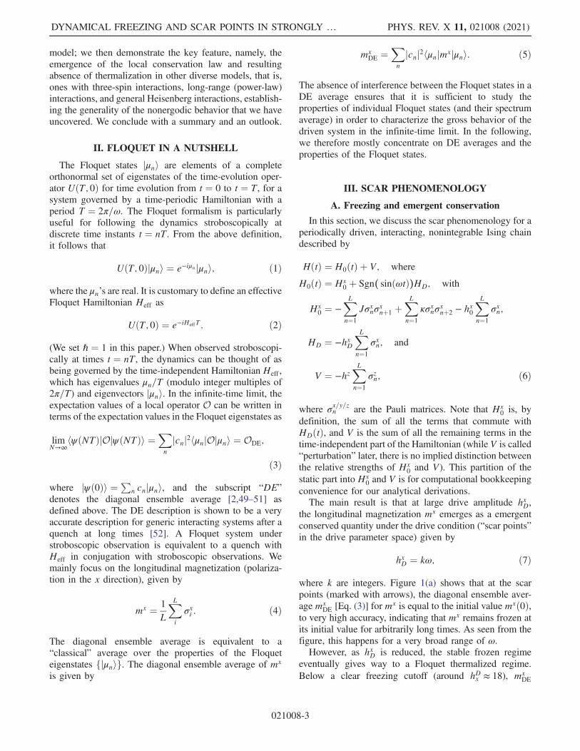
where k are integers. Figure 1(a) shows that at the scarpoints (marked with arrows), the diagonal ensemble aver-age mx

DE [Eq. (3)] for mx is equal to the initial value mxð0Þ,to very high accuracy, indicating that mx remains frozen atits initial value for arbitrarily long times. As seen from thefigure, this happens for a very broad range of ω.However, as hxD is reduced, the stable frozen regime

eventually gives way to a Floquet thermalized regime.Below a clear freezing cutoff (around hDx ≈ 18), mx

DE

DYNAMICAL FREEZING AND SCAR POINTS IN STRONGLY … PHYS. REV. X 11, 021008 (2021)

021008-3

exhibits strong fluctuations as a function of hxD (shortfrozen stretches punctuated by higher-order resonance;see Sec. V B 1), followed by a subsequent sharp declineto almost zero below a thermalization threshold (aroundhxD ≈ 5). A locally infinite-temperature-like Floquet ther-malized regime is observed below this threshold, as shownin Fig. 1(b). This threshold does not exhibit any perceptibleshift with system size [38]. The inset of Fig. 1(b) shows thatthere is no perceptible L dependence in the freezing ofmx

DEas long as hxD is above the freezing cutoff. The phenomenonis reminiscent of the nonmonotonic peak-valley structure offreezing observed in integrable Floquet systems in thethermodynamic limit [39,40].The figure shows that freezing happens for two very

different kinds of initial states, namely, the highly polarizedinitial ground state of Hð0Þ as well as a high-temperaturethermal state. The initial thermal density matrix is of theform

ρThðt ¼ 0Þ ¼X2Lj¼1

e−βεj

Zjεjihεjj; ð8Þ

where jεji is the jth eigenstate of an initial HamiltonianHI , with eigenvalue εj. We have chosen HI ¼ Hðt ¼ 0;hxD ¼ 5.0; hx0 ¼ 0.1; J ¼ 1; κ ¼ 0.7Þ, with HðtÞ fromEq. (6), and Z ¼ P

j e−βεj is the partition function.

Equation (8) represents a mixture of eigenstates jεji.Hence, we obtain the final diagonal ensemble densitymatrix by summing the diagonal ensemble density matrix

for each jεji, weighted by its Boltzmann weight in ρThð0Þ,i.e.,

ρDEðt → ∞Þ ¼Xj

e−βεj

Z

�Xk

jhεjjμkij2jμkihμkj�

¼Xk

�Xj

e−βεj

Zjhεjjμkij2

�jμkihμkj: ð9Þ

The emergent conservation of mx for a generic thermalstate suggests that all the Floquet states must be organizedaccording to the conservation law. This case is shown tobe true in Fig. 1(c), which displays the expectation valuehmxi in the Floquet eigenstates [corresponding to thedrive in Fig. 1(c)], plotted against their serial number(normalized by the dimension DH of the Hilbert space),arranged in decreasing order of their hmxi values. For thescar points, for hxD ¼ 40 at ω ¼ 10, 20, 40, the values ofhmxi of the Floquet states coincide with the eigenvaluesof mx, indicating that all the eigenstates of mx thatparticipate in a given Floquet state have the same mx

eigenvalues. This result explains the conservation orfreezing of mx for dynamics starting with any genericinitial state. As we will see later, the condition forencountering such a scar point [Eq. (7)] can be deducedfrom both the FDPT and a Magnus expansion in a time-dependent frame, and the latter confirms the effect overthe entire spectrum and explains the steps in hmxi to theleading orders.

(a) (b) (c)

FIG. 1. Scars, resonances, and emergent conservation law. (a) mxDE=m

x0, the ratio of magnetizations after infinite (diagonal ensemble

average) and 0 (initial state) cycles versus drive frequency ω. Freezing, reflected in a large value of this ratio, occurs over a broadrange of ω and is strongest at particular “scar” points (marked with arrows) hxD ¼ kω, where k is an integer (for hxD ¼ −40 here, the tenarrows mark ω ¼ 40=k; k ¼ 1; 2;…; 10). Results are shown for zero and high-temperature initial states: the former being theground state ofHð0Þ [which gives an initial magnetizationmxð0Þ≲ 1], and the latter being the Gibbs state with β ¼ 10−2 [mxð0Þ ≈ 0.05]for HI of the form Hð0Þ but with hxD ¼ 5; all other parameters are the same as the driven Hamiltonian, namely, J ¼ 1;κ ¼ 0.7π=3; hx0 ¼ e=10; hxD ¼ 40; hz ¼ 1.2; L ¼ 14. The sharp dips in the green lines represent resonances, discussed in detail inthe main text on Floquet-Dyson perturbation theory. Parameters are chosen to avoid these resonances. (b) mx as a function of hxD for afixed ratio jhxD=ωj ¼ 4, showing the freezing cutoff ðhxD ≈ 18Þ above which a stable regime of freezing sets in. Inset: finite-size behaviorof the freezing. For intermediate strengths of the driving field, higher-order resonances lead to nonmonotonic behavior of mx

DE on L,which is then sensitively dependent on small variations of hxD. (c) hmxi of the Floquet states plotted against the serial number(normalized by the Hilbert space dimension DH) of the Floquet states, arranged in decreasing order of hmxi. At the scar points (ω ¼ 10,20, and 40), the hmxi values form steps coinciding with the eigenvalues of mx arranged and plotted in the same order: mx emerges as aemergent conserved quantity, hence the freezing of mx for any generic initial state.

HALDAR, SEN, MOESSNER, and DAS PHYS. REV. X 11, 021008 (2021)

021008-4

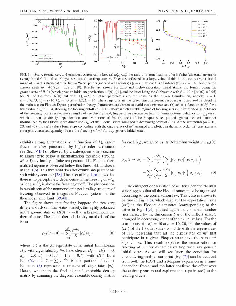
B. Dynamics of the unentangled eigenstates of mx:Growth of entanglement entropy

We define an unentangled, complete, orthonormal set ofeigenstates of mx, which we call the x basis. Each elementof the x basis is a simultaneous eigenstate of all the σxioperators. The nontriviality of the dynamics at the scarpoints and the consequence of the emergent conservationare manifested in the growth of the half-chain entanglemententropy E1

2at the scar points, especially with different x-

basis eigenstates of mx as initial states. We study the half-chain entanglement entropy

E12¼ −Tr½ρ1

2log2ρ1

2�; ð10Þ

where ρ12is the density matrix of one half of the chain,

obtained by tracing out the other half.The results are shown in Fig. 2. These results highlight

that, even though mx is conserved for large enough hxD atthe scar points, there is substantial dynamics even at thosepoints. For large enough hxD, Figs. 2(d)–2(i), we see thatdifferent eigenstates of mx evolve quite differently even atthe scar points, at which mx is conserved to a very goodapproximation for all initial states. For example, for thefully polarized initial state, entanglement does not groweven after 1010 drive cycles, but for the Neel and the L=2-domain-pair initial states, it does. This reflects the respec-tive sizes of the mx subspaces with maximal and zeromagnetization.

(a)

(d)

(g) (h) (i)

(e) (f)

(b) (c)

FIG. 2. (De)localization of the wave function over the x basis (simultaneous eigenstates of all of the σxi ’s) as evidenced by the half-chain entanglement entropy (E1

2) versus system size L, for different driving strengths hxD (rows) and initial states (left column: maximally

mx polarized; middle: L=2-domain-pair state with vanishing total mx; right: Neel state). Top row (small hxD ¼ 5): E12entropy grows

linearly with system size for all initial states, signaling ergodicity. For stronger drives (hxD ¼ 20 and 40 in the middle and bottom rows,respectively), scars appear, and E1

2depends strongly on the initial states, reflecting the size of the emergent magnetization sectors: For the

fully polarized initial states (left column), E12does not grow at all for the freezing or scar points [marked as (F) in the figure legends

and represented by almost indistinguishably coincidental black and violet triangles], while for the Neel and the L=2-domain-pair initialstates, there is considerable growth in E1

2even at the scar points, reflecting (at least partial) delocalization over the large concomitant

magnetization sectors. The results are for J ¼ 1; κ ¼ 0.7; hx0 ¼ e=10; hz ¼ 1.2; L ¼ 14, averaged over 104 cycles after driving for 1010

cycles.

DYNAMICAL FREEZING AND SCAR POINTS IN STRONGLY … PHYS. REV. X 11, 021008 (2021)

021008-5

The growth of E12also reflects the role of interactions in

the dynamics even at the scar points, without which wewould not see such a substantial growth of entanglement.In the Appendix C, we show that the suppression of

entanglement growth is robust in that it is observed forother patterns of the drive field, as long as the concomitantemergent conservation law gives rise to well-definedsectors that contain only a small number of states.

IV. STRONG-DRIVE MAGNUS EXPANSION

We next provide a modified Magnus expansion thatincorporates the large size of the drive from the start, usingthe inverse of the driving field as a small parameter. Thisapproach makes the emergence of a conserved quantitymanifest, for a wide range of Hamiltonians—the terms inthe time-independent part of the Hamiltonian that commutewith the time-dependent part of the Hamiltonian (Hx

0 here)can have any form because the factor premultiplying theterms involving Hx

0 vanishes to second order regardless ofthe form of Hx

0. For example, it applies to transverse-fieldIsing models in any dimension, with any Ising interaction.Using this approach, one can immediately read off the scarsfound above.The conventional Magnus expansion uses the inverse

of a large frequency as a small parameter (see, e.g.,Refs. [28,53]) for obtaining the Floquet HamiltonianHeff [Eq. (2)] as given below.

Heff ¼X∞n¼0

HðnÞF ; where

Hð0ÞF ¼ 1

T

ZT

0

dtHðtÞ;

Hð1ÞF ¼ 1

2!ðiÞTZ

T

0

dt1

Zt1

0

dt2½Hðt1Þ; Hðt2Þ�; ð11Þ

and so on. In our case, we have hxD > ω, making theseries nonconvergent even when ω is greater than allother couplings in the Hamiltonian, so the naïve Magnusexpansion is qualitatively wrong even at leading order: Thefirst-order term Hð0Þ is the time average over one period ofHðtÞ [Eq. (6)], an interacting, generic Hamiltonian thatdoes not conservemx. Hence, we would have no hint of thescars even from the first-order term.This problem can be remedied when the strong drive

modulates the strength of a fixed field or potential (this is avery natural way of applying a periodic drive). The largestcoupling (hxD here) can be eliminated from the Hamiltonianby switching to a time-dependent frame as follows [28]. Weintroduce a unitary transformation

jψmovðtÞi ¼ WðtÞ†jψðtÞi;Omov ¼ WðtÞ†OWðtÞ; ð12Þ

where jψðtÞi is the wave function and O is any predefinedoperator (the subscript “mov” marks the quantities in themoving frame).The crux of the expansion is then apparent for a WðtÞ of

the following form,

WðtÞ ¼ exp

�−i

Zt

0

dt0rðt0ÞHD

�; ð13Þ

where rðtÞ is a T-periodic parameter. If the totalHamiltonian were constant up to the time-dependentprefactor rðtÞ, i.e., HðtÞ ¼ rðtÞHð0Þ, the above wouldjust give the solution of the static Schrödinger equation,but with a rate of phase accumulation for each (time-independent) eigenstate given by the integrand of thevariable prefactor. In particular, any conservation law ofHð0Þ would be bequeathed to the time-dependent problem.Now, if the drive is not the only, but still the dominantpart of the Hamiltonian, there will be corrections to thispicture; however, this suggests the eigenbasis of the driveand its conservation law(s) should remain perturbativelyuseful starting points.Given the form of HDðtÞ in Eq. (6), the transformed

Hamiltonian reads

Hmov ¼ WðtÞ†HðtÞWðtÞ − iWðtÞ†∂tW; ð14Þ

where the second term exactly cancels the part from thefirst term that has hxD as its coupling; hence, Hmov is freefrom any coupling of order hxD (see Appendix A 3 fordetails).

A. Scars in the driven interacting Ising chain

In the case of Eq. (6), we have

HðtÞ ¼ Hx0 þ V − Sgn(sin ðωtÞ)hxD

Xi

σxi : ð15Þ

Switching to the moving frame by using the transformationin Eq. (13) gives

Hmov ¼ Hx0 − hz

Xi

½cos ð2θÞσzi þ sin ð2θÞσyi �; where

θðtÞ ¼ −hxD

Zt

0

dt0Sgnðsinωt0Þ: ð16Þ

After some algebra, we find the Magnus expansion ofHmovto have the following leading terms:

Hð0ÞF ¼ Hx

0 −hz

hxDT

�sin ðhxDTÞ

Xi

σzi

− (1 − cos ðhxDTÞ)Xi

σyi

�: ð17Þ

HALDAR, SEN, MOESSNER, and DAS PHYS. REV. X 11, 021008 (2021)

021008-6

Note that this is useful for hxD ≫ 1=T, the regime we areinterested in. The next-order term is given by

Hð1ÞF ¼ 1

2!Ti

ZT

0

dt1

Zt1

0

dt2½Hmovðt1Þ; Hmovðt2Þ�: ð18Þ

Denoting θðt1Þ ¼ θ1, θðt2Þ ¼ θ2,P

i σz=yi ¼ Sz=y, and the

form of Hmov from Eq. (16), we get

Hð1ÞF ¼ ½Sz;Hx

0�hzðcos 2θ2 − cos 2θ1Þþ ½Sy;Hx

0�hzðsin 2θ2 − sin 2θ1Þþ ½Sy; Sz�ðhzÞ2 sinð2θ1 − 2θ2Þ: ð19Þ

Upon integration (see Appendix A 1 and A 3 for details),this identically gives

Hð1ÞF ¼ 0: ð20Þ

The end result—a homogeneous expansion in the smallparameters 1=hxD and 1=T from the two initial orders—given in Eq. (17), is quite remarkable. First, for hxDT ¼ 2πk

(where k can be any integer), Hð0ÞF ¼ Hx

0; this is preciselythe condition for scars observed numerically [Eq. (7)]and also from the FDPT [see Eq. (44)]. Clearly, to thisapproximation, Heff not only has a conservation law but isalso integrable; indeed, it is classical, with all termscommuting. Numerical results suggest that the aboveexpansion (unlike the Magnus expansion in the staticframe) is an asymptotic one, at least in the neighborhoodof the scar points, since the leading-order terms representthe exact numerical results accurately.

Second, it is clear from the forms of Hð0ÞF and Hð1Þ

F thatthe results hold independently of the form of Hx

0; thiscould be in any spatial dimension and can incorporate anyform of Ising interactions. This wide generality impliesthat stable emergent conservation laws and constraints (inkeeping with the possible asymptotic nature of theexpansion) may emerge in generic interacting Floquetsystems in the thermodynamic limit. Since H0

x is, bydefinition, the portion of the static part of the Hamiltonianthat commutes with HD, the statement of generalityobtained from the above analysis stands as follows:While the nature of the whole static part can be tunedover a wide variety of many-body Hamiltonians depend-ing on the form of Hx

0 (ranging from noninteracting tointeracting, integrable to nonintegrable, low to highdimensional), the emergence of the conservation lawand the resultant scarring do not depend on the form ofHx

0. In Sec. VI, we support this statement by consideringvarious kinds of Ising interactions, and going beyond, wedemonstrate the freezing in the presence of anisotropicHeisenberg interactions.

V. FLOQUET-DYSON PERTURBATION THEORY

In this section, we develop a theory that opens awindow on the otherwise difficult-to-access [46–48] low-frequency regime. We first test it for an exactly solubleproblem and then apply it to the Ising chain studied in theprevious section.We find that the theory provides valuable insights for

both systems. In particular, it identifies a resonance con-dition corresponding to the dips, as well as a freezingcondition corresponding to the maxima in the responseplotted in Figs. 4 and 1, respectively. A concurrence of thetwo accounts for the varying dip depths in that figure.While a comprehensive treatment of the general many-body problem is not yet possible, we believe that theseitems capture ingredients central for its understanding.We first present the general formulation of the FDPT.

The goal is to construct the Floquet states jμni. We resortto a setting where the unperturbed Hamiltonian is timedependent and the perturbation is static [54]. The centralidea is to construct the Floquet states in the presence of thesmall static perturbation from the known unperturbedFloquet states by applying time-dependent perturbationtheory (a Dyson-like series for the wave function). For thisprocess, one needs to know the unperturbed Floquet states,which come from the solution of the time-dependentSchrödinger equation with only the time-dependent partin the Hamiltonian (including the static parts that commutewith it at all times). In our case, this is naturally achievedas follows. The central ingredient is that the drivenHamiltonian

HðtÞ ¼ H0ðtÞ þ V ð21Þ

contains a large time-dependent term H0ðtÞ, which has atime-independent set of eigenstates and a perturbation Vthat is time independent. Those states then serve as theunperturbed Floquet states, and V can then be treated as asmall (compared to the drive amplitude) perturbation.We work in the basis of eigenstates of H0ðtÞ (these are

the unperturbed Floquet states), denoted as jni, so that

H0ðtÞjni ¼ EnðtÞjni; ð22Þ

and hmjni ¼ δmn.Next, we assume, without loss of generality, that V is

completely off-diagonal in this basis, namely,

hnjVjni ¼ 0 ð23Þ

for all n. We now find solutions of the time-dependentSchrödinger equation

i∂jψni∂t ¼ HðtÞjψnðtÞi; ð24Þ

DYNAMICAL FREEZING AND SCAR POINTS IN STRONGLY … PHYS. REV. X 11, 021008 (2021)

021008-7

which satisfy

jψnðTÞi ¼ e−iμn jψnð0Þi: ð25Þ

For V ¼ 0, each eigenstate jni of H0ðtÞ is a Floquet

state, with Floquet quasienergy μð0Þn ¼ RT0 dtEnðtÞ (defined

modulo 2π).For V nonzero but small, we develop a Dyson-like series

for the wave function to first order in V. Clearly, V is asmall perturbation as long as jV=hxDj ≪ 1, though it canotherwise be comparable to or larger than the othercouplings of the undriven Hamiltonian. In our ansatz,the nth eigenstate is written as

jψnðtÞi ¼Xm

cmðtÞe−iR

t

0dt0Emðt0Þjmi; ð26Þ

where cnðtÞ ≃ 1 for all t while cmðtÞ is of order V (andtherefore small) for all m ≠ n and all t.We then substitute the form for the wave function in

Eq. (26) in the time-dependent Schrödinger equation andthen apply the key condition of the method; namely, wedemand jψnð0Þi ¼ jμni, i.e.,

jψnðTÞi ¼ eiμn jψnð0Þi: ð27Þ

Then, taking the overlaps with the basis states jmi, we find(for details of the algebra, see Appendix B)

cmð0Þ ¼ −ihmjVjniRT0 dtei

Rt

0dt0½Emðt0Þ−Enðt0Þ�

eiR

T

0dt½EmðtÞ−EnðtÞ� − 1

: ð28Þ

We see that cmðtÞ is indeed of order V provided that thedenominator on the right-hand side of Eq. (28) does notvanish; we call this case nondegenerate. If

eiR

T

0dt½EmðtÞ−EnðtÞ� ¼ 1; ð29Þ

we have a resonance between states jmi and jni, and theabove analysis breaks down. Now, if there are several statesthat are connected to jni by the perturbation V, Eq. (28)describes the amplitude to go to each of them from jni. Upto order V2, the total probability of excitation away from jniis given by

Pm≠n jcmð0Þj2 at time t ¼ 0.

A. Single large spin: An exactly soluble test bed

As a simple illustration of the FDPT, we discuss asystem with a single spin governed by a time-dependentHamiltonian. We briefly discuss some results obtainedfrom the FDPT (which give the conditions for perfectfreezing and resonances), numerical results, and exactresults for the Floquet operator. The details are presentedin Appendix B.

1. Model

We consider a single spin S, with S2 ¼ SðSþ 1Þ, whichis governed by a Hamiltonian of the form

HðtÞ ¼ −hxSx − hzSz − hxDSgn(sinðωtÞ)Sx: ð30Þ

The time period is T ¼ 2π=ω. Since sinðωtÞ is positive for0 < t < T=2 and negative for T=2 < t < T, the Floquetoperator is given by

U ¼ eðiT=2Þ½ðhx−hxDÞSxþhzSz� × eðiT=2Þ½ðhxþhxDÞSxþhzSz�: ð31Þ

It is clear from the group properties of matrices of the form

eia·S thatU in Eq. (31) must be of the same form and can bewritten as

U ¼ eiγk·S;

where k ¼ ðcos θ; sin θ cosϕ; sin θ sinϕÞ: ð32Þ

We work in the basis in which Sx is diagonal. Since theeigenstates of U in Eq. (32) are the same as the eigenstatesof the matrix M ¼ k · S, the expectation values of Sx inthe different eigenstates take the values cos θ timesS; S − 1;…;−S. The maximum expectation value is givenby mx

max ¼ S cos θ.

2. Analytical results from FDPT

We can use the FDPT to derive the correction to mxmax to

first order in the small parameter hz=hxD. Namely, we findhow the state given by j0i≡ jSx ¼ Si mixes with the statej1i≡ jSx ¼ S − 1i. We discover that

c1ð0Þ ¼ffiffiffiffiffiffi2S

phz

hxD

eihxT=2½eihxDT=2 − cosðhxT=2Þ�

eihxT − 1

: ð33Þ

Three possibilities arise at this stage.(i) The denominator of Eq. (33) is not zero. Then,

the expectation value of Sx in this state will be closeto S since hz=hxD is small. In addition, if thenumerator of Eq. (33) vanishes, we get perfectfreezing, namely, hSxi ¼ S.

(ii) The denominator of Eq. (33) vanishes; i.e., hx is aninteger multiple of 2π=T, but the numerator doesnot vanish. This is called the resonance condition.Clearly, the perturbative result for c1ð0Þ breaksdown in this case, and we have to either developa degenerate perturbation theory or do an exactcalculation.

(iii) Both the numerator and the denominator of Eq. (33)vanish. Once again, the perturbative result breaksdown, and we have to do a more careful calculation.

Here, we comment on the dependence of the result inEq. (33) on the value of S. At t ¼ 0, the probability of state

HALDAR, SEN, MOESSNER, and DAS PHYS. REV. X 11, 021008 (2021)

021008-8

j1i is jc1ð0Þj2, and the probability of state j0i is1 − jc1ð0Þj2. Hence, the expectation value of Sx=S isgiven by

mxmax

S¼ 1

S½Sð1 − jc1ð0Þj2Þ þ ðS − 1Þjc1ð0Þj2�

¼ 1 − 2

�hz

hxD

�2

×1þ cos2ðhxT=2Þ − 2 cos ðhxT=2Þ cos ðhxDT=2Þ

4 sin2ðhxT=2Þ :

ð34Þ

We expect Eq. (33) to break down at a sufficiently largevalue of S since it was derived using first-order perturbationtheory, which is accurate only if jc1ð0Þj ≪ 1. However, weobserve that the value of mx

max=S in Eq. (34) is independentof S. Therefore, in this model, we have the striking resultthat we can use first-order perturbation theory for values ofS that are not large to derive an expression like Eq. (34),which is then found to hold for arbitrarily large values of S.

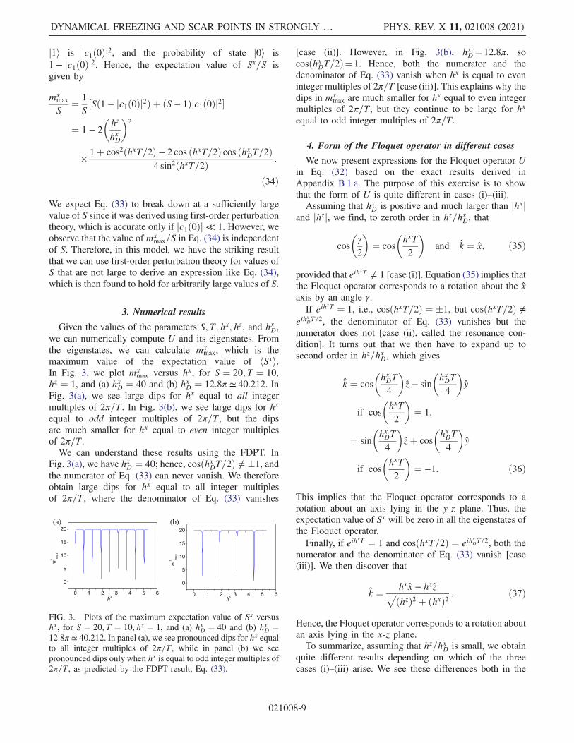
3. Numerical results

Given the values of the parameters S; T; hx; hz, and hxD,we can numerically compute U and its eigenstates. Fromthe eigenstates, we can calculate mx

max, which is themaximum value of the expectation value of hSxi.In Fig. 3, we plot mx

max versus hx, for S ¼ 20; T ¼ 10;hz ¼ 1, and (a) hxD ¼ 40 and (b) hxD ¼ 12.8π ≃ 40.212. InFig. 3(a), we see large dips for hx equal to all integermultiples of 2π=T. In Fig. 3(b), we see large dips for hx

equal to odd integer multiples of 2π=T, but the dipsare much smaller for hx equal to even integer multiplesof 2π=T.We can understand these results using the FDPT. In

Fig. 3(a), we have hxD ¼ 40; hence, cosðhxDT=2Þ ≠ �1, andthe numerator of Eq. (33) can never vanish. We thereforeobtain large dips for hx equal to all integer multiplesof 2π=T, where the denominator of Eq. (33) vanishes

[case (ii)]. However, in Fig. 3(b), hxD¼12.8π, socosðhxDT=2Þ¼1. Hence, both the numerator and thedenominator of Eq. (33) vanish when hx is equal to eveninteger multiples of 2π=T [case (iii)]. This explains why thedips in mx

max are much smaller for hx equal to even integermultiples of 2π=T, but they continue to be large for hx

equal to odd integer multiples of 2π=T.

4. Form of the Floquet operator in different cases

We now present expressions for the Floquet operator Uin Eq. (32) based on the exact results derived inAppendix B 1 a. The purpose of this exercise is to showthat the form of U is quite different in cases (i)–(iii).Assuming that hxD is positive and much larger than jhxj

and jhzj, we find, to zeroth order in hz=hxD, that

cos

�γ

2

�¼ cos

�hxT2

�and k ¼ x; ð35Þ

provided that eihxT ≠ 1 [case (i)]. Equation (35) implies that

the Floquet operator corresponds to a rotation about the xaxis by an angle γ.If eih

xT ¼ 1, i.e., cosðhxT=2Þ ¼ �1, but cosðhxT=2Þ ≠eih

xDT=2, the denominator of Eq. (33) vanishes but the

numerator does not [case (ii), called the resonance con-dition]. It turns out that we then have to expand up tosecond order in hz=hxD, which gives

k ¼ cos

�hxDT4

�z − sin

�hxDT4

�y

if cos

�hxT2

�¼ 1;

¼ sin

�hxDT4

�zþ cos

�hxDT4

�y

if cos

�hxT2

�¼ −1: ð36Þ

This implies that the Floquet operator corresponds to arotation about an axis lying in the y-z plane. Thus, theexpectation value of Sx will be zero in all the eigenstates ofthe Floquet operator.Finally, if eih

xT ¼ 1 and cosðhxT=2Þ ¼ eihxDT=2, both the

numerator and the denominator of Eq. (33) vanish [case(iii)]. We then discover that

k ¼ hxx − hzzffiffiffiffiffiffiffiffiffiffiffiffiffiffiffiffiffiffiffiffiffiffiffiffiffiffiðhzÞ2 þ ðhxÞ2

p : ð37Þ

Hence, the Floquet operator corresponds to a rotation aboutan axis lying in the x-z plane.To summarize, assuming that hz=hxD is small, we obtain

quite different results depending on which of the threecases (i)–(iii) arise. We see these differences both in the

0 1 2 3 4 5 6

0

5

10

15

20

mx m

ax

hx 0 1 2 3 4 5 6

0

5

10

15

20

mx m

ax

hx

(a) (b)

FIG. 3. Plots of the maximum expectation value of Sx versushx, for S ¼ 20; T ¼ 10; hz ¼ 1, and (a) hxD ¼ 40 and (b) hxD ¼12.8π ≃ 40.212. In panel (a), we see pronounced dips for hx equalto all integer multiples of 2π=T, while in panel (b) we seepronounced dips only when hx is equal to odd integer multiples of2π=T, as predicted by the FDPT result, Eq. (33).

DYNAMICAL FREEZING AND SCAR POINTS IN STRONGLY … PHYS. REV. X 11, 021008 (2021)

021008-9

numerical results for mxmax shown in Fig. 3 and in the forms

of the Floquet operator in Eqs. (35)–(37), which areobtained by an exact calculation.

B. FDPT for the interacting Ising chain

Now, we apply FDPT to our interacting Ising chain[Eq. (6)], studied numerically above. We set hz ≪ hxD, andtreat V as the perturbation. We use periodic boundaryconditions.The eigenstates jni of H0ðtÞ are diagonal in the basis of

the operators σxn. In particular, the state in which all spinsσxn ¼ þ1 will be denoted as j0i, and we start by calculatingthe Floquet state jmx

maxi (maximally polarized Floquetstate) obtained by perturbing this state to first order inhz=hxD. While calculating mx from perturbation theory, weuse this Floquet state.The rationale for this is as follows. First, if we start with a

fully polarized state in the þx direction (as is done, forexample, in the experiments by Monroe [55]) or with theground state of Hð0Þ, with hxD ≫ hz; κ, then the initial stateis expected to have a strong overlap with this particularFloquet state. Hence, at very long times, the expectationvalues of the observables in the wave function will be wellapproximated by the expectation value in this Floquet state.Second, in this setting, the insights from the single-spin

problem studied above are most directly transferable; inparticular, we again encounter the ideas of resonances andscars. With these in hand, we can then identify a number offeatures present in the data more generally, in particular, forhigh-temperature states (which are of interest in the contextof the NMR experiments by Rovny [56]). We find thatperturbation theory works best in the vicinity of the scarswith their emergent integrability (see below), and wepresent a limited exploration of the performance ofFDPT away from these in Appendix B.For the expansion of the Floquet state to leading order,

the computation proceeds entirely along the lines of thatpresented for the single-spin model. We denote the state inwhich all spins σxn ¼ þ1, except for the site m whereσxm ¼ −1, as jmi. In the limit in which hxD is much largerthan J, κ, and hx0, we find that, to leading order in hz=hxD,Eq. (B24) takes the form

cmð0Þ ≃hz

hxD

eiAT=2½eihxDT − cosðAT=2Þ�eiAT − 1

;

A ¼ 4ðJ − κÞ þ 2hx0: ð38ÞThe magnetization of this maximally polarized Floquet

state is given as follows. The expectation value ofP

Ln¼1 σ

xn

in each of the m states is L − 2, and in the state j0i, it is L.This gives

mx ¼ 1 −2

L

XLm¼1

jcmð0Þj2: ð39Þ

1. Resonances and stability of the scar

The resonance condition [Eqs. (29) and (38)],

eiAT ¼ 1 where A ¼ 4ðJ − κÞ þ 2hx0; ð40Þ

signals the singularities of our expansion, where cmð0Þdiverges. For our Hamiltonian, this occurs for

hx0 ¼ −2J þ 2κ þ pω2

: ð41Þ

Here, p is an integer that corresponds to the number ofphotons absorbed or emitted in this transition. Thus, ourfirst-order theory does not preclude multiphoton transitions.This suggests considering all possible first-order reso-

nances based on Eq. (29), by considering the resonancecondition more generally: Evaluating the change Em − Endue to the flip of only a single spin, σ0, with nth nearest-neighbor spins on the right or left denoted by σ�n, yields thefirst-order resonance condition

hx0σ0 þ Jσ0ðσ−1 þ σ1Þ − κσ0ðσ−2 þ σ2Þ ¼pω2

: ð42Þ

Of course, individual resonances may be absent if there areno matrix elements between the states in question.This approach can be rather successful at identifying the

locations of the numerically observed isolated resonances,as displayed in Fig. 4. There, the strength of the freezing isdisplayed as a function of driving strength, for both slowand very slow drives, ω ¼ 0.4 and 0.04, respectively.The right panel of Fig. 4 emphasizes the generality

of this result: The considerations of the first-order reso-nances obtained above yield the response even for theinitially weakly polarized (mx ¼ 0.05), high-temperatureinitial state.For a many-body Floquet system, a proliferation of

Floquet resonances may lead to unbounded heating. Hence,a stable nonthermal state (e.g., a scar) a priori requires theabsence of resonances. Equation (42) shows that this isstraightforwardly possible to first order since the resonan-ces are isolated and can be well separated in parameterspace. This stems from the fact that the gap Em − Enbetween two distinct (possibly degenerate) levels of Hx

0

[Eq. (6)] does not necessarily vanish even in the thermo-dynamic limit (for example, if we take all the couplings inHx

0 to be rational numbers). The absence of any signature ofthe higher-order resonances in the exact numerical result atvery low frequencies (ω ¼ 0.04) and large hxD ¼ 40 in theneighborhoods of the scar points indicates that the first-order theory is sufficient there, and the FDPT series is atleast asymptotic in nature.Higher-order resonances start gaining importance as hxD

is reduced below a freezing cutoff (hxD ≈ 18), as shown inFig. 1(b). The choice of parameters rules out first-orderresonances in this case. The results are consistent with this

HALDAR, SEN, MOESSNER, and DAS PHYS. REV. X 11, 021008 (2021)

021008-10

when the drive amplitude is above the cutof—we see noresonant dip in mx

DE. But as hxD is tuned below the cutoff,

rapid irregular fluctuations appear due to sharp resonantdips in mx

DE. With the first-order resonances being ruledout, these dips are due to higher-order resonances, whichimplies that first-order perturbation theory is insufficientbelow the cutoff. With further lowering of hDx , a sharp dropto the Floquet thermalized regime mx

DE ∼ 0 eventuallyappears below a threshold (hxD ≈ 5).

Scar from FDPT.—Considering the expression for themagnetization, obtained by substituting the expressionfor cmð0Þ [Eq. (38)] into the expression of mx [Eq. (39)],

1 −mx ¼ 2

�hz

hxD

�2

×1þ cos2ðAT=2Þ − 2 cosðAT=2Þ cosðhxDTÞ

4 sin2ðAT=2Þ ;

ð43Þ

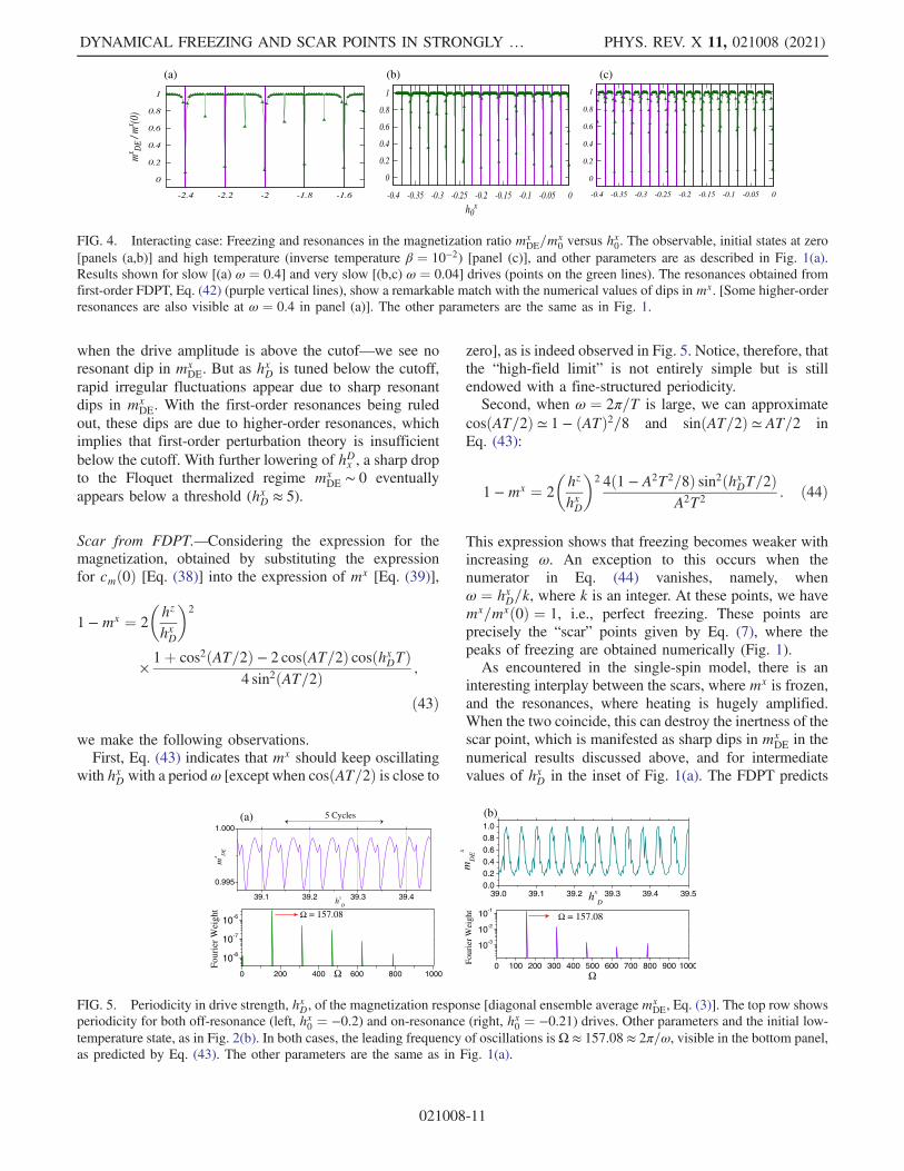
we make the following observations.First, Eq. (43) indicates that mx should keep oscillating

with hxD with a periodω [except when cosðAT=2Þ is close to

zero], as is indeed observed in Fig. 5. Notice, therefore, thatthe “high-field limit” is not entirely simple but is stillendowed with a fine-structured periodicity.Second, when ω ¼ 2π=T is large, we can approximate

cosðAT=2Þ ≃ 1 − ðATÞ2=8 and sinðAT=2Þ ≃ AT=2 inEq. (43):

1 −mx ¼ 2

�hz

hxD

�2 4ð1 − A2T2=8Þ sin2ðhxDT=2Þ

A2T2: ð44Þ

This expression shows that freezing becomes weaker withincreasing ω. An exception to this occurs when thenumerator in Eq. (44) vanishes, namely, whenω ¼ hxD=k, where k is an integer. At these points, we havemx=mxð0Þ ¼ 1, i.e., perfect freezing. These points areprecisely the “scar” points given by Eq. (7), where thepeaks of freezing are obtained numerically (Fig. 1).As encountered in the single-spin model, there is an

interesting interplay between the scars, where mx is frozen,and the resonances, where heating is hugely amplified.When the two coincide, this can destroy the inertness of thescar point, which is manifested as sharp dips in mx

DE in thenumerical results discussed above, and for intermediatevalues of hxD in the inset of Fig. 1(a). The FDPT predicts

39.1 39.2 39.3 39.4

0.995

1.000

hx

D

mx D

E

5 Cycles

0 200 400 600 800 1000

10-8

10-7

10-6

Ω

Four

ier

Wei

ght Ω = 157.08

39.0 39.1 39.2 39.3 39.4 39.50.00.20.40.60.81.0

mD

E

x

hx

D

0 100 200 300 400 500 600 700 800 900 1000

10-3

10-2

10-1

Fou

rier

Wei

ght

Ω

Ω = 157.08

(a) (b)

FIG. 5. Periodicity in drive strength, hxD, of the magnetization response [diagonal ensemble averagemxDE, Eq. (3)]. The top row shows

periodicity for both off-resonance (left, hx0 ¼ −0.2) and on-resonance (right, hx0 ¼ −0.21) drives. Other parameters and the initial low-temperature state, as in Fig. 2(b). In both cases, the leading frequency of oscillations is Ω ≈ 157.08 ≈ 2π=ω, visible in the bottom panel,as predicted by Eq. (43). The other parameters are the same as in Fig. 1(a).

(a) (b) (c)

FIG. 4. Interacting case: Freezing and resonances in the magnetization ratio mxDE=m

x0 versus h

x0. The observable, initial states at zero

[panels (a,b)] and high temperature (inverse temperature β ¼ 10−2) [panel (c)], and other parameters are as described in Fig. 1(a).Results shown for slow [(a) ω ¼ 0.4] and very slow [(b,c) ω ¼ 0.04] drives (points on the green lines). The resonances obtained fromfirst-order FDPT, Eq. (42) (purple vertical lines), show a remarkable match with the numerical values of dips in mx. [Some higher-orderresonances are also visible at ω ¼ 0.4 in panel (a)]. The other parameters are the same as in Fig. 1.

DYNAMICAL FREEZING AND SCAR POINTS IN STRONGLY … PHYS. REV. X 11, 021008 (2021)

021008-11

isolated resonances in parameter space and provides aguide for choosing the Hamiltonian parameters to avoidresonances and observe stable scars. Our choice of param-eters for Fig. 1 is guided by the theory [Eq. (42)], and weindeed observe resonance-free strong freezing at the scarpoints.It would clearly be desirable to embark on a more

detailed study, both with respect to the role of higher-orderresonances (visible in the left panel of Fig. 4) and withregard to the statistics of the resonances as the system sizeincreases.

VI. ROBUSTNESS AND GENERALITY OF THESCARRING AND EMERGENT CONSERVATION

In this section, we demonstrate the robustness andgenerality of the phenomenon of emergent conservationand the consequent absence of thermalization, by compar-ing the diagonal ensemble average mx

DE with the drivingfrequency ω for a range of qualitatively distinct models. Wealso demonstrate the stability of the conservation law at thescar or freezing points upon increasing the system size. Inall cases, the drive strength is set to be hxD ¼ 40, and thefreezing peaks or scar points are thus expected to occur forω ¼ 40=k, where k is an integer. This condition wasderived for all Ising interactions in Sec. IV and will bederived for general two-body Heisenberg interactions inSec. VI B.

A. Additional forms of Ising interactions

First, we confirm, as predicted by the moving-frameMagnus expansion in Sec. IV, the robustness of thephenomenon under diverse variations of the form of Hx

0

in the total Hamiltonian partitioned in the form of Eq. (6).We recall that Hx

0 is the portion of the static part of theHamiltonian that commutes with HD, and the nature ofthe whole static part can be tuned over a wide variety ofmany-body Hamiltonians depending on the form of Hx

0,ranging from noninteracting to interacting, integrable tononintegrable, and low to high dimensional. We considertwo forms for Hx

0. First, we add a three-body interaction, ofstrength Jxxx,

Hxð3SpinÞ0 ¼ −J

Xi

σxi σxiþ1 þ κ

Xi

σxi σxiþ2

þ JxxxXi

σxi σxiþ1σ

xiþ2 − hx0

XLi

σxi : ð45Þ

Second, we consider long-range interactions as follows.Spins are placed equidistantly on a circle, and the distancerij between the ith and the jth spin is measured along thechord connecting them, such that

HxðLRÞ0 ¼ −J

Xij

σxi σxj

rij− hx0

XLi

σxi : ð46Þ

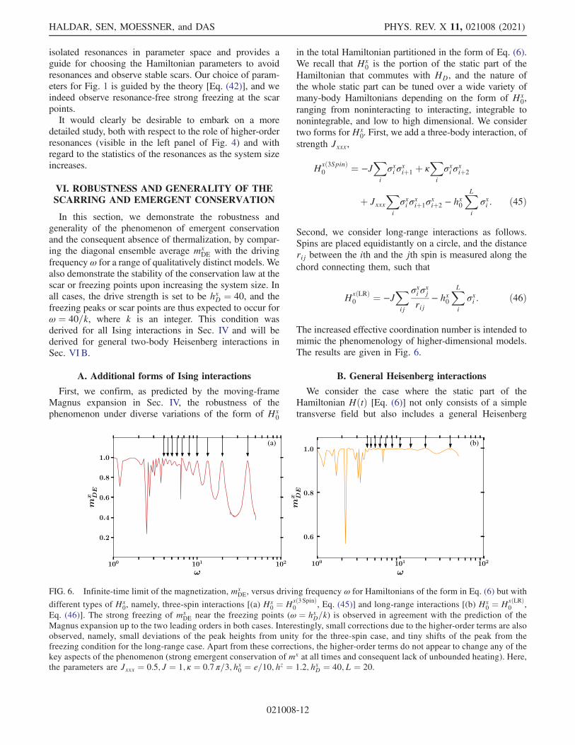
The increased effective coordination number is intended tomimic the phenomenology of higher-dimensional models.The results are given in Fig. 6.

B. General Heisenberg interactions

We consider the case where the static part of theHamiltonian HðtÞ [Eq. (6)] not only consists of a simpletransverse field but also includes a general Heisenberg

(a) (b)

FIG. 6. Infinite-time limit of the magnetization, mxDE, versus driving frequency ω for Hamiltonians of the form in Eq. (6) but with

different types of Hx0, namely, three-spin interactions [(a) Hx

0 ¼ Hxð3 SpinÞ0 , Eq. (45)] and long-range interactions [(b) Hx

0 ¼ HxðLRÞ0 ,

Eq. (46)]. The strong freezing of mxDE near the freezing points (ω ¼ hxD=k) is observed in agreement with the prediction of the

Magnus expansion up to the two leading orders in both cases. Interestingly, small corrections due to the higher-order terms are alsoobserved, namely, small deviations of the peak heights from unity for the three-spin case, and tiny shifts of the peak from thefreezing condition for the long-range case. Apart from these corrections, the higher-order terms do not appear to change any of thekey aspects of the phenomenon (strong emergent conservation of mx at all times and consequent lack of unbounded heating). Here,the parameters are Jxxx ¼ 0.5; J ¼ 1; κ ¼ 0.7 π=3; hx0 ¼ e=10; hz ¼ 1.2; hxD ¼ 40; L ¼ 20.

HALDAR, SEN, MOESSNER, and DAS PHYS. REV. X 11, 021008 (2021)

021008-12

interaction with arbitrary position dependence. TheHeisenberg terms involving σy;zi are included in the Vterm, and those involving σxi are included in the H

0x term as

follows. The total HamiltonianHðtÞ ¼ HHBðtÞ, in this case,has the same form in Eq. (6) but with V replaced by

VHB ¼ −Xi;j

Jyijσyi σ

yj −

Xi;j

Jzijσziσ

zj − hz

Xi

σz ð47Þ

and Hx0 replaced by

HxðHBÞ0 ¼ −

Xi;j

Jxijσxi σ

xj þ κ

Xσxi σ

xiþ2 − hx0

Xσxi : ð48Þ

The total static Hamiltonian V þHx0 can thus have a

general Heisenberg term with an arbitrary interaction graph(coordination number, spatial dimensionality, and positiondependence).

For the changed form of V, the moving frame Magnusexpansion requires some additional lengthy steps (seeAppendix A 2) but eventually leads to the same conclusionas derived in Sec. IV; namely, mx is exactly conserved inthe first two orders of the expansion.Interestingly, the first term (zeroth order in 1=ω) exhibits

an attractive route to the emergent conserved quantity: Allthe terms, in addition to Hx

0, do not in fact vanish, buttheir sum explicitly exhibits a U(1) symmetry presentneither in HðtÞ nor in HmovðtÞ. This assures conservationofmx in the first order. In the next order (first order in 1=ω),all the terms except Hx

0 vanish. In the following, wesummarize the results, relegating the detailed calculationto Appendix A 1.For the total Hamiltonian HHBðtÞ, employing the unitary

transformation induced byWðtÞ [Eq. (13)], we switch to themoving frame, in which our total Hamiltonian reads

HmovHB ðtÞ ¼ Hx

0 −Xi;j

Jyijσyi σ

yj

�I cos2ð2θÞ − σxi σ

xjsin

2ð2θÞ þ i2sinð4θÞðσxi þ σxjÞ

�

−Xi;j

Jzijσziσ

zj

�I cos2ð2θÞ − σxi σ

xjsin

2ð2θÞ þ i2sinð4θÞðσxi þ σxjÞ

�

− hz cosð2θÞXi

σzi þ hz sinð2θÞXi

σyi : ð49Þ

In the following, we state the results of the Magnusexpansion of Hmov

HB ðtÞ.The first term (zeroth order in 1=ω) is the average

Hamiltonian, given by

Hð0Þeff ¼

1

T

ZT

0

dtHmovHB ðtÞ

¼ HxðHBÞ0 −

1

2

Xi;j

ðJyij þ JzijÞ½σyi σyj þ σziσzj�; ð50Þ

under the freezing condition hxDT ¼ 2πk (or hxD ¼ kω).This term, though nontrivial and nonzero, is visibly U(1)symmetric and commutes with mx.The second term (first order in 1=ω) reads

Hð1Þeff ¼

1

2!ðiÞTZ

T

0

dt1

Zt1

0

dt2½HmovHB ðt1Þ; Hmov

HB ðt2Þ�: ð51Þ

Using Eq. (49), calculating all the commutators, andperforming the integrals (see Appendix A 2), we finallyget, under the freezing condition hxDT ¼ 2πk,

Hð1Þeff ¼ 0; ð52Þ

which finally yields

Heff ¼ HxðHBÞ0 −

1

2

Xi;j

ðJyij þ JzijÞ½σyi σyj þ σziσzj�; ð53Þ

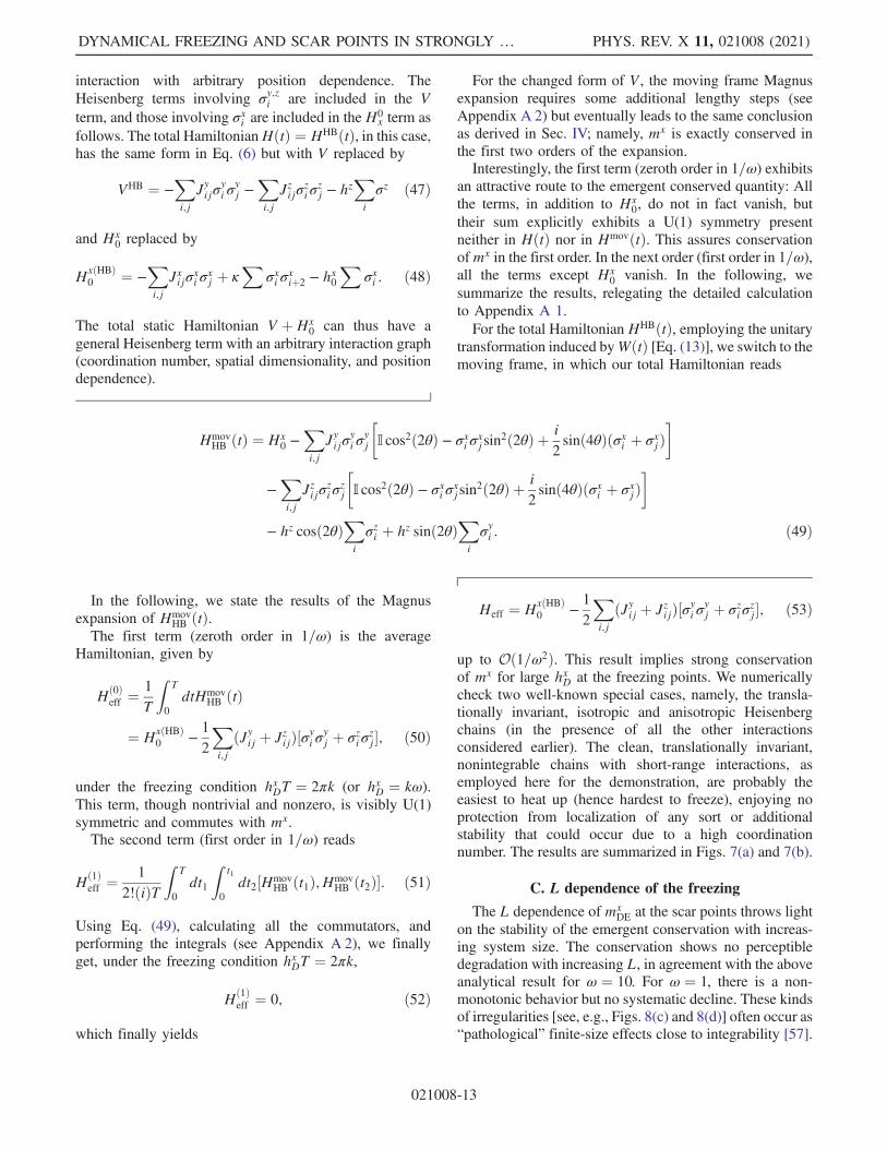
up to Oð1=ω2Þ. This result implies strong conservationof mx for large hxD at the freezing points. We numericallycheck two well-known special cases, namely, the transla-tionally invariant, isotropic and anisotropic Heisenbergchains (in the presence of all the other interactionsconsidered earlier). The clean, translationally invariant,nonintegrable chains with short-range interactions, asemployed here for the demonstration, are probably theeasiest to heat up (hence hardest to freeze), enjoying noprotection from localization of any sort or additionalstability that could occur due to a high coordinationnumber. The results are summarized in Figs. 7(a) and 7(b).

C. L dependence of the freezing

The L dependence of mxDE at the scar points throws light

on the stability of the emergent conservation with increas-ing system size. The conservation shows no perceptibledegradation with increasing L, in agreement with the aboveanalytical result for ω ¼ 10. For ω ¼ 1, there is a non-monotonic behavior but no systematic decline. These kindsof irregularities [see, e.g., Figs. 8(c) and 8(d)] often occur as“pathological” finite-size effects close to integrability [57].

DYNAMICAL FREEZING AND SCAR POINTS IN STRONGLY … PHYS. REV. X 11, 021008 (2021)

021008-13

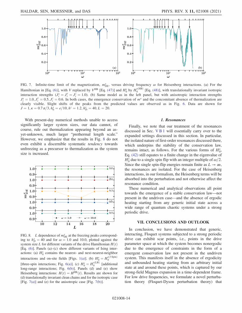
With present-day numerical methods unable to accesssignificantly larger system sizes, our data cannot, ofcourse, rule out thermalization appearing beyond an as-yet-unknown, much larger “prethermal length scale.”However, we emphasize that the results in Fig. 8 do noteven exhibit a discernible systematic tendency towardsunfreezing as a precursor to thermalization as the systemsize is increased.

1. Resonances

Finally, we note that our treatment of the resonancesdiscussed in Sec. V B 1 will essentially carry over to theexpanded settings discussed in this section. In particular,the isolated nature of first-order resonances discussed there,which underpins the stability of the conservation law,remains intact, as follows. For the various forms of Hx

0,Eq. (42) still equates to a finite change in the eigenvalue ofHx

0 due to a single spin flip with an integer multiple of ω=2.Since the single spin-flip energies remain finite as L → ∞,the resonances are isolated. For the case of Heisenberginteractions, in our formalism, the Heisenberg terms will beabsorbed into the perturbation and not otherwise affect theresonance condition.These numerical and analytical observations all point

towards the emergence of a stable conservation law—notpresent in the undriven case—and the absence of ergodicheating starting from any generic initial state across awide range of quantum chaotic systems under a strongperiodic drive.

VII. CONCLUSIONS AND OUTLOOK

In conclusion, we have demonstrated that generic,interacting, Floquet systems subjected to a strong periodicdrive can exhibit scar points, i.e., points in the driveparameter space at which the system becomes nonergodicdue to the emergence of constraints in the form of aemergent conservation law not present in the undrivensystem. This manifests itself in the absence of ergodicityand unbounded heating starting from an arbitrary initialstate at and around these points, which is captured by ourstrong-field Magnus expansion in a time-dependent frame.For low drive frequencies, we formulate a novel perturba-tion theory (Floquet-Dyson perturbation theory) that

(a)

(b)

(c)

(d)

(e)

FIG. 8. L dependence of mxDE at the freezing peaks correspond-

ing to hxD ¼ 40 and for ω ¼ 1.0 and 10.0, plotted against thesystem size L for different variants of the drive Hamiltonian HðtÞ[Eq. (6)]. Panels (a)–(c) show different variants of Ising inter-actions: (a) Hx

0 contains the nearest- and next-nearest-neighbor

interactions and on-site fields [Figs. 1(a)]. (b) Hx0 ¼ Hxð3SpinÞ

0

[three-spin interactions; Fig. 6(a)]. (c) Hx0 ¼ HxðLRÞ

0 [additionallong-range interactions; Fig. 6(b)]. Panels (d) and (e) showHeisenberg interactions: HðtÞ ¼ HHBðtÞ. Results are shown for(d) translationally invariant clean chains and for the isotropic case[Fig. 7(a)] and (e) for the anisotropic case [Fig. 7(b)].

(a) (b)

FIG. 7. Infinite-time limit of the magnetization, mxDE, versus driving frequency ω for Heisenberg interactions. (a) For the

Hamiltonian in [Eq. (6)], with V replaced by VHB [Eq. (47)] and Hx0 by HxðHBÞ

0 [Eq. (48)], with translationally invariant isotropicinteraction strengths (Jxi ¼ Jyi ¼ Jzi ¼ 1.0). (b) Same model as in the left panel, but with anisotropic interaction strengthsJxi ¼ 1.0; Jyi ¼ 0.5; Jzi ¼ 0.6. In both cases, the emergence conservation of mx and the concomitant absence of thermalization areclearly visible. Slight shifts of the peaks from the predicted values are observed as in Fig. 6. Data are shown forJ ¼ 1; κ ¼ 0.7 π=3; hx0 ¼ e=10; hz ¼ 1.2; hxD ¼ 40; L ¼ 20.

HALDAR, SEN, MOESSNER, and DAS PHYS. REV. X 11, 021008 (2021)

021008-14

works, even at first order, very accurately at or nearintegrability of the scar points. In particular, the resonancespredicted by the theory accurately coincide with the sharpdips in the emergent conserved quantity. At the resonances,the system absorbs energy without bound from the drive,and hence the scars “compete” with the resonances. Theresonances predicted by the theory appear to be isolated inparameter space, and thus, the theory provides a guidelinefor choosing parameters for observing resonance-freestable scars, as we demonstrate here. These results hold,in particular, for Ising systems in any dimension and withany form of the Ising interactions, as well as in the presenceof additional pairwise Heisenberg interactions forming anarbitrary interaction graph. We also demonstrate the robust-ness of the phenomenon in the presence of anisotropicHeisenberg (XYZ) interactions.The exact mechanism of this many-body phenomenon

is actually still unknown, and the intuitions we havegathered are based on renormalization of the couplings,which are most effectively revealed under the nonpertur-bative, time-dependent frame transformation. For certainvalues of parameters, these renormalization factors vanishowing to destructive many-body quantum interference.These features are not captured by ordinary (lab-frame)Magnus expansion because it misses the effective resum-mation necessary for these factors to manifest, as per-formed by the frame transformation.The emergence and stability of a conservation law in an

interacting, quantum, chaotic many-body system due tostrong periodic drive is an unexpected and intriguingphenomenon, which warrants extensive investigations. Oneimportant direction is to study the nature of the state throughcontinuous (nonstroboscopic) time—the so-called micromo-tions. A powerful technique to study this is the so-called vanVleck expansion (also known as the “high-frequency expan-sion” see, e.g., Refs. [28,53,58] and references therein) of theFloquet Hamiltonian. This method is also a potential alter-native to our approach to study the stroboscopic problem.Our work also touches on various Floquet experiments.

In the original experimental work on Floquet many-bodylocalization [31], the interest in a large drive was alreadynoted. In the context of the studies of Floquet time crystals,the two kinds of states studied above have also played acentral role: The trapped ion experiment [55] used a fullypolarized starting state, while the NMR experiment [56]employed a high-temperature state.Our work points towards the important role in non-

equilibrium settings played by the generation of emergentconservation laws and constraints, in contrast to onlyfocusing on those existing in the static (undriven) system,and their demise under an external drive. Our work alsoopens a door for stable Floquet engineering in interactingsystems and indicates a recipe for tailoring interesting statesand structured Hilbert spaces by choosing suitable driveHamiltonians.

ACKNOWLEDGMENTS

A. D. thanks Subinay Dasgupta and SirshenduBhattacharyya for collaborating on a noninteracting versionof the phenomenon studied here [40]. We acknowledgeuseful discussions with Marin Bukov. The QuSpin PYTHON

package [59,60] was used in this work. This researchwas supported in part by the International Centre forTheoretical Sciences (ICTS) during a visit for the programThermalization, Many Body Localization andHydrodynamics (Code: ICTS/hydrodynamics2019/11).A. D. and A. H. acknowledge the partner group program“Spin liquids: Correlations, dynamics and disorder”between IACS and MPI-PKS, and the visitors programof MPI-PKS for supporting visits to PKS during thecollaboration. This research was, in part, supported bythe Deutsche Forschungsgemeinschaft under the cluster ofexcellence EXC2147 ct.qmat (Project No. 39085490) anddeveloped with funding from the Defense AdvancedResearch Projects Agency (DARPA) via the DRINQSprogram. The views, opinions, and/or findings expressedare those of the authors and should not be interpretedas representing the official views or policies of theDepartment of Defense or the U.S. Government. R. M.is grateful to Vedika Khemani, David Luitz, and ShivajiSondhi for collaboration on related work [61]. D. S. thanksDST, India, Project No. SR/S2/JCB-44/2010, for financialsupport.

APPENDIX A: STRONG-FIELD FLOQUETEXPANSION

1. Ising case

Here, we provide the details of the derivation of theeffective Hamiltonian in Eqs. (17)–(20). Carrying out thePauli algebra gives

Hmov ¼ Hx0 − hz

Xi

½cos ð2θÞσzi þ sin ð2θÞσyi �; where

θðtÞ ¼ −hxD

Zt

0

dt0Sgnðsinωt0Þ: ðA1Þ

We note that the frame change does not affect mx since itcommutes with WðtÞ.Next, we perform the Magnus expansion of Hmov. The

initial orders are given by

Heff ¼X∞n¼0

H0F; where

Hð0ÞF ¼ 1

T

ZT

0

HmovðtÞdt;

Hð1ÞF ¼ 1

2!iT

ZT

0

dt1

Zt1

0

dt2½Hmovðt1Þ; Hmovðt2Þ�; ðA2Þ

DYNAMICAL FREEZING AND SCAR POINTS IN STRONGLY … PHYS. REV. X 11, 021008 (2021)

021008-15

etc. We first consider the term Hð0ÞF . It is easy to check that

Hx0 remains unaffected by the rotation, and the integrals in

the first term vanish, giving

Hð0ÞF ¼ Hx

0: ðA3Þ

Next, we consider the second-order term

Hð1ÞF ¼ 1

2!ðiÞTZ

T

0

dt1

Zt1

0

dt2½Hðt1Þ; Hðt2Þ�: ðA4Þ

Arranging the terms in the commutator, we get

½Hðt1Þ; Hðt2Þ� ¼ K1 þ K2 þ K3; where

K1 ¼ −hzfcos (θðt2Þ) − cos (θðt1Þ)g½Hx0;Sz�;

K2 ¼ −hzfsin (θðt2Þ) − sin (θðt1Þ)g½Hx0;Sy�;

K3 ¼ ðhzÞ2 sin ½θðt2Þ − θðt1Þ�½Sz;Sy�; ðA5Þ

where Sx=y=z ¼P

Li σ

x=y=zi .

Next, we note that the integral in Eq. (A4) can be brokenup in the following way,

I½f(θðt1Þ;θðt2Þ)�¼Z

T

0

dt1

Zt1

0

dt2½f(θðt1Þ;θðt2Þ)�

¼ I1½f(θðt1Þ;θðt2Þ)�þI2½f(θðt1Þ;θðt2Þ)�;þI3½f(θðt1Þ;θðt2Þ)�; where

I1½f(θðt1Þ;θðt2Þ)�¼Z

T=2

0

dt1

Zt1

0

dt2½f(θðt1Þ;θðt2Þ)�;

I2½f(θðt1Þ;θðt2Þ)�¼Z

T

T=2dt1

ZT=2

0

dt2½f(θðt1Þ;θðt2Þ)�;

I3½f(θðt1Þ;θðt2Þ)�¼Z

T

T=2dt1

Zt1

T=2dt2½f(θðt1Þ;θðt2Þ)�:

ðA6Þ

Finally, we note that

For I1; θðt1Þ ¼ −hxDt1; θðt2Þ ¼ −hxDt2;

For I2; θðt1Þ ¼ −hxDðT − t1Þ; θðt2Þ ¼ −hxDt2;

For I3; θðt1Þ ¼ −hxDðT − t1Þ; θðt2Þ ¼ −hxDðT − t2Þ:ðA7Þ

Using Eqs. (A4)–(A7) and evaluating the integrals,we obtain Eqs. (17)–(20) (see Appendix A 3 for furtherdetails).

2. Heisenberg case

In the Heisenberg case, the total Hamiltonian HðtÞ ¼HHBðtÞ has the same form as that in Eq. (6), except with Vreplaced by

VHB ¼ −Xi;j

Jyijσyi σ

yj −

Xi;j

Jzijσziσ

zj − hz

Xi

σz ðA8Þ

and Hx0 replaced by

HxðHBÞ0 ¼ −Jxij

Xσxi σ

xj þ κ

Xσxi σ

xiþ2 − hx0

Xσxi : ðA9Þ

Now, following Sec. IV, we switch to the moving frameby acting on the total HamiltonianHHBðtÞ, with the unitarytransformation given by

VðtÞ ¼ exp

�ihxD

Xj

σxj

Zt

t0

Sgn(sinðωt0Þ)dt0�

¼Yj

exp

�ihxDσ

xj

Zt

t0

Sgn(sinðωt0Þ)dt0�; ðA10Þ

where

θðtÞ ¼ hxD

Zt

t0

Sgn(sinðωt0Þ)dt0: ðA11Þ

This transformation gives our moving-frame Hamiltonian

HmovHB ðtÞ ¼

Yi

exp½−iσxi θðtÞ�H0 exp½iσxi θðtÞ�

¼ HxðHBÞ0 −

Yi

exp ½−iσxi θðtÞ��X

k;l

Jyk;lσykσ

yl

�Yj

exp ½iσxjθðtÞ� −Yi

exp ½−iσxi θðtÞ��X

k;l

Jzk;lσzkσ

zl

�Yj

exp ½iσxjθðtÞ�

− hzYi

exp ½−iσxi θðtÞ��X

k;l

σzk

�Yj

exp ½iσxjθðtÞ�; ðA12Þ

where

HxðHBÞ0 ¼ −Jxij

Xσxi σ

xj þ κ

Xσxi σ

xiþ2 − hx0

Xσxi ; ðA13Þ

which gives

HALDAR, SEN, MOESSNER, and DAS PHYS. REV. X 11, 021008 (2021)

021008-16

HmovHB ðtÞ ¼ HxðHBÞ

0 −Xk;l

Jyk;le−iσxkθðtÞe−iσ

xl θðtÞðσykσyl Þeiσ

xkθðtÞeiσ

xl θðtÞ

−Xk;l

Jzk;le−iσxkθðtÞe−iσ

xl θðtÞðσzkσzl Þeiσ

xkθðtÞeiσ

xl θðtÞ − hz

Xk;l

e−iσxkθðtÞσzke

iσxkθðtÞ: ðA14Þ

The Jyij term can be simplified to

¼ −Xi;j

Jyijσyi σ

yje

2iσxi θðtÞe2iσxjθðtÞ

¼ −Xi;j

Jyijσyi σ

yj ½I cos2ð2θÞ − σxi σ

xj sin

2ð2θÞ þ i sinð2θÞ cosð2θÞðσxi þ σxjÞ�: ðA15Þ

Similarly, the Jzij term becomes

¼ −Xi;j

Jzijσziσ

zj½I cos2ð2θÞ − σxi σ

xj sin

2ð2θÞ þ i sinð2θÞ cosð2θÞðσxi þ σxjÞ�: ðA16Þ

The hz term is similar to our previous case, namely,

¼ −hz cosð2θÞXi

σzi þ hz sinð2θÞXi

σyi : ðA17Þ

Hence,

HmovHB ðtÞ ¼ HxðHBÞ

0 −Xi;j

Jyijσyi σ

yj

�I cos2ð2θÞ − σxi σ

xjsin

2ð2θÞ þ i2sinð4θÞðσxi þ σxjÞ

�

−Xi;j

Jzijσziσ

zj

�I cos2ð2θÞ − σxi σ

xjsin

2ð2θÞ þ i2sinð4θÞðσxi þ σxjÞ

�

− hz cosð2θÞXi

σzi þ hz sinð2θÞXi

σyi : ðA18Þ

Next, we perform the Magnus expansion on Eq. (A18).The zeroth-order term is

Hð0Þeff ¼

1

T

ZT

0

dtHmovHB ðtÞ: ðA19Þ

Now, with the definition of θðtÞ given in Eq. (A11), we getZ

T

0

cos2ð2θÞdt ¼ T2þ sin 2hxDT

4hDx; ðA20aÞ

ZT

0

sin2ð2θÞdt ¼ T2−sin 2hxDT4hDx

; ðA20bÞZ

T

0

sinð4θÞdt ¼ 1

4hDxð1 − cos 2hxDTÞ; ðA20cÞ

ZT

0

sinð2θÞdt ¼ 1

hDxð1 − cos hxDTÞ; ðA20dÞ

ZT

0

cosð2θÞdt ¼ 1

hxDsinðhxDTÞ: ðA20eÞ

Applying the freezing condition,

hxDT ¼ 2πn; ðA21Þ

we get

ZT

0

cos2ð2θÞdt ¼ T2; ðA22aÞ

ZT

0

sin2ð2θÞdt ¼ T2; ðA22bÞ

ZT

0

sinð4θÞdt ¼ 0; ðA22cÞZ

T

0

sinð2θÞdt ¼ 0; ðA22dÞZ

T

0

cosð2θÞdt ¼ 0: ðA22eÞ

Putting everything in Eq. (A19), we obtain

DYNAMICAL FREEZING AND SCAR POINTS IN STRONGLY … PHYS. REV. X 11, 021008 (2021)

021008-17

Hð0Þeff ¼ HxðHBÞ

0 −Xi;j

Jyijσyi σ

yj1

T

�T2− σxi σ

xjT2

�

−Xi;j

Jzijσziσ

zj1

T

�T2− σxi σ

xjT2

�ðA23Þ

¼ HxðHBÞ0 −

1

2

Xi;j

½σyi σyj þ σziσzj�ðJyij þ JzijÞ: ðA24Þ

We already have

½HxðHBÞ0 ; mx� ¼ 0;

and one can easily show that

�Xi;j

ðσyi σyj þ σziσzjÞ; mx

�¼ 0: ðA25Þ

The first-order term of the Magnus expansion is

Hð1Þeff ¼

1

2!Ti

ZT

0

dt1

Zt1

0

dt2½HmovHB ðt1Þ; Hmov

HB ðt2Þ�: ðA26Þ

Rearranging all the terms in Eq. (A18), we can write

HmovHB ðtÞ ¼ HxðHBÞ

0 þ A cos2ð2θÞ þ B sin2ð2θÞþ C sinð4θÞ þD cosð2θÞ þ E sinð2θÞ: ðA27Þ

Hence,

½HmovHB ðt1Þ;Hmov

HB ðt2Þ� ¼ ½HxðHBÞ0 ;A�I1 þ ½HxðHBÞ

0 ;B�I2 þ ½HxðHBÞ0 ;C�I3 þ ½HxðHBÞ

0 ;D�I4 þ ½HxðHBÞ0 ;E�I5 þ ½A;B�I6 þ ½A;C�I7

þ ½A;D�I8 þ ½A;E�I9 þ ½B;C�I10 þ ½B;D�I11 þ ½B;E�I12 þ ½C;D�I13 þ ½C;E�I14 þ ½D;E�I15;ðA28Þ

where

A ¼ −Xi;j

½Jyijσyi σyj þ Jzijσziσ

zj�; B ¼

Xi;j

½ðJyijσyi σyj þ Jzijσziσ

zjÞσxi σxj �; C ¼ −

Xi;j

i2½ðJyijσyi σyj þ Jzijσ

ziσ

zjÞðσxi þ σxjÞ�;

D ¼ −hzXi

σzi ; and E ¼ hzXi

σyi ; ðA29Þ

and

I1 ¼ cos2(2θðt2Þ)− cos2(2θðt1Þ);I2 ¼ sin2(2θðt2Þ)− sin2(2θðt1Þ);I3 ¼ sin(4θðt2Þ)− sin(4θðt1Þ);I4 ¼ cos(2θðt2Þ)− cos(2θðt1Þ);I5 ¼ sin(2θðt2Þ)− sin(2θðt1Þ);I6 ¼ cos2(2θðt1Þ)sin2(2θðt2Þ)− sin2(2θðt1Þ)cos2(2θðt2Þ);I7 ¼ cos2(2θðt1Þ)sin(4θðt2Þ)− sin(4θðt1Þ)cos2ð2θðt2Þ);I8 ¼ cos2(2θðt1Þ)cos(2θðt2Þ)− cos(2θðt1Þ)cos2ð2θðt2Þ);I9 ¼ cos2(2θðt1Þ)sin(2θðt2Þ)− sin(2θðt1Þ)cos2ð2θðt2Þ);I10¼ sin2(2θðt1Þ)sin(4θðt2Þ)− sin(4θðt1Þ)sin2ð2θðt2Þ);I11¼ sin2(2θðt1Þ)cos(2θðt2Þ)− cos(2θðt1Þ)sin2ð2θðt2Þ);I12¼ sin2(2θðt1Þ)sin(2θðt2Þ)− sin(2θðt1Þ)sin2ð2θðt2Þ);I13¼ sin(4θðt1Þ)cos(2θðt2Þ)− cos(2θðt1Þ)sin4θðt2Þ;I14¼ sin(4θðt1Þ)sin(2θðt2Þ)− sin(2θðt1Þ)sin(4θðt2Þ);I15¼ sin½2(θðt1Þ−θðt2Þ)�: ðA30Þ

Now, one can show that all 15 integrals of In in Eq. (A30)vanish for the freezing condition. Hence,

Heff ¼ HxðHBÞ0 −

1

2

Xi;j

½σyi σyj þ σziσzj�ðJyij þ JzijÞ

up to the first two orders.

3. Explicit calculation of the integrals in the movingframe Magnus expansion: Ising case (self-contained)

The Hamiltonian can be written as

HðtÞ ¼ H0 þ rðtÞHD: ðA31Þ

We move to the rotating frame using the transformation

HmovðtÞ ¼ W†ðtÞH0WðtÞ; ðA32Þ

where the rotation operator is

WðtÞ ¼ exp

�−i

Zt

t0

rðt0Þdt0HD

�: ðA33Þ

HALDAR, SEN, MOESSNER, and DAS PHYS. REV. X 11, 021008 (2021)

021008-18

The first case is an Ising model with next-nearest-neighborterms:

H0 ¼ −Xi

Jσxi σxiþ1 þ κ

Xσxi σ

xiþ2 − hx0

Xσxi − hz

Xσzi ;

ðA34Þ

¼ Hx0 þ V ðA35Þ

HD ¼ −hxDX

σxi ; ðA36Þ

and

rðtÞ ¼ Sgn(sinðωtÞ): ðA37Þ

From Eqs. (A33), (A36), and (A37), we get

WðtÞ ¼ exp

�ihxD

Xj

σxj

Zt

t0

Sgn(sinðωt0Þ)dt0�

¼Yj

exp

�ihxDσ

xj

Zt

t0

Sgn(sinðωt0Þ)dt0�: ðA38Þ

Defining

θðtÞ ¼ −hxD

Zt

t0

Sgn(sinðωt0Þ)dt0; ðA39Þ

and putting all of these together, we get

HmovðtÞ ¼Yi

exp½−iσxi θðtÞ�H0 exp½iσxi θðtÞ�

¼ Hx0 − hz

Yi

exp ½−iσxi θðtÞ��X

k

σzk

�

×Yj

exp ½iσxjθðtÞ� ðA40Þ

¼ Hx0 − hz

Xk

e−iσxkθðtÞσzke

iσxkθðtÞ ðA41Þ

∴ HmovðtÞ ¼ Hx0 − hz cos 2θ

Xi

σzi − hz sin 2θXi

σyi :

ðA42Þ

Now, we can perform Magnus expansion on Eq. (A42).The zeroth-order term is

Hð0Þeff ¼

1

T

ZT

0

HmovðtÞdt

¼ 1

T

ZT

0

Hx0dt −

hz

T

Xi

σzi

ZT

0

cos 2θdt

−hz

T

Xi

σyi

ZT

0

sin 2θdt: ðA43Þ

Then, with the definition of θðtÞ as given in Eq. (A39)[note: θðtÞ ¼ −hxDt for 0 < t ≤ ðT=2Þ, and θðtÞ ¼−ðhxDT − hxDtÞ for ðT=2Þ ≤ t ≤ T], the integralsimplifies to

ZT

0

cos2θdt¼Z T

2

0

cos2θdtþZ

T

T2

cos2θdt

¼Z T

2

0

cos ð2hxDtÞdtþZ

T

T2

cos2ðhxDT − hxDtÞdt

¼ 1

hxDsin ðhxDTÞ: ðA44Þ

Similarly,

ZT

0

sin 2θdt ¼ 1

hxD(cos ðhxDTÞ − 1): ðA45Þ

Putting Eqs. (A44) and (A45) into Eq. (A43), we get

Hð0Þeff ¼ Hx

0 −hz

hxDT

Xi

σzi sin ðhxDTÞ

þ hz

hxDT

Xi

σyi (1 − cos ðhxDTÞ): ðA46Þ

Now, putting the freezing condition hxDT ¼ 2nπ inEq. (A46), i.e., sin hxDT ¼ 0 and cos hxDT ¼ 1, one gets

Hð0Þeff jfreezing ¼ Hx

0: ðA47Þ

Next, we evaluate the first-order term,

Hð1Þeff ¼

1

2!Ti

ZT

0

dt1

Zt1

0

dt2½Hmovðt1Þ; Hmovðt2Þ�: ðA48Þ

Calling θðt1Þ ¼ θ1; θðt2Þ ¼ θ2 andP

i σzi ¼ Sz;P

i σyi ¼ Sy and using the form of Hmov from Eq. (A42),

the commutator in Eq. (A48) simplifies to

½Hmovðt1Þ; Hmovðt2Þ� ¼ ½Sz;Hx0�hzðcos 2θ2 − cos 2θ1Þ

þ ½Sy;Hx0�hzðsin 2θ2 − sin 2θ1Þ

þ ½Sy; Sz�ðhzÞ2 sinð2θ1 − 2θ2Þ:ðA49Þ

DYNAMICAL FREEZING AND SCAR POINTS IN STRONGLY … PHYS. REV. X 11, 021008 (2021)

021008-19

Now, for example, the integral corresponding to the first term is

I1 ¼Z

T

0

Zt1

0

dt1dt2ðcos 2θ2 − cos 2θ1Þ ðA50Þ

¼Z T

2

0

dt1

Zt1

0

dt2 cos 2θðt2Þ þZ

T

T2

dt1

Z T2

0

dt2 cos 2θðt2Þ þZ

T

T2

dt1

Zt1

T2

dt2 cos 2θðt2Þ −Z

T

0

dt1 cos 2θðt1Þt1

¼Z T

2

0

dt1

Zt1

0

dt2 cosð2hxDt2Þ þZ

T

T2

dt1

Z T2

0

dt2 cosð2hxDt2Þ þZ

T

T2

dt1

Zt1

T2

dt2 cosð2hxDT − 2hxDt2Þ

−Z T

2

0

dt1t1 cosð2hxDt1Þ −Z

T

T2

dt1t1 cosð2hxDT − 2hxDt1Þ; ðA51Þ

I1 ¼ IA1 þ IB1 þ IC1 − ID1 − IE1 : ðA52Þ

Then,

IA1 ¼Z T

2

0

dt1

Zt1

0

dt2 cosð2hxDt2Þ ¼1

2hxD

Z T2

0

dt1 sin 2hxDt1 ¼1

ð2hxDÞ2½1 − cos hxDT�; ðA53Þ

IB1 ¼Z

T

T2

dt1

Z T2

0

dt2 cosð2hxDt2Þ ¼1

2hxD

ZT

T2

dt1 sin hxDT ¼ T4hxD

sin hxDT; ðA54Þ

IC1 ¼Z

T

T2

dt1

Zt1

T2

dt2 cosð2hxDT − 2hxDt2Þ ¼1

2hxD

ZT

T2

dt1½sin hxDT − sinð2hxDT − 2hxDt1Þ�

¼ T4hxD

sin hxDT −1

ð2hxDÞ2þ 1

ð2hxDÞ2cos hxDT; ðA55Þ

ID1 ¼Z T

2

0

dt1t1 cosð2hxDt1Þ ¼1

2hxD

�T2sin hxDT −

Z T2

0

dt1 sin 2hxDt1

�

¼ T4hxD

sin hxDT þ 1

ð2hxDÞ2cos hxDT −

1

ð2hxDÞ2; ðA56Þ

IE1 ¼Z

T

T2

dt1t1 cosð2hxDT − 2hxDt1Þ ¼T4hxD

sin hxDT þ 1

2hxD

ZT

T2

dt1 sinð2hxDT − 2hxDt1Þ

¼ T4hxD

sin hxDT þ 1

ð2hxDÞ2ð1 − cos hxDTÞ: ðA57Þ

Now, putting Eqs. (A53)–(A57) into Eq. (A52) yields

I1 ¼ 0: ðA58Þ

Carrying out the integrals corresponding to the other twocommutators in Eq. (A49), one can similarly get

I2 ¼Z

T

0

Zt1

0

dt1dt2ðsin 2θ1 − sin 2θ2Þ ¼ 0; ðA59Þ

I3 ¼Z

T

0

Zt1

0

dt1dt2 sinð2θ1 − 2θ2Þ ¼ 0: ðA60Þ

APPENDIX B: FLOQUET-DYSONPERTURBATION THEORY

We start from Eq. (24), which implies that

iXm

_cmðtÞe−iR

t

0dt0Emðt0Þjmi

¼ VXm

cmðtÞe−iR

t

0dt0Emðt0Þjmi; ðB1Þ

where the dot over cm denotes d=dt. Taking the innerproduct of Eq. (B1) with hnj and using Eq. (23), we find, tofirst order in V, that

HALDAR, SEN, MOESSNER, and DAS PHYS. REV. X 11, 021008 (2021)

021008-20

_cn ¼ 0: ðB2Þ

We can therefore choose

cnðtÞ ¼ 1 ðB3Þfor all t. We thus have

jψnðtÞi ¼ e−iR

t

0dt0Enðt0Þjni þ

Xm≠n

cmðtÞe−iR

t

0dt0Emðt0Þjmi:

ðB4ÞHence, Eq. (25) implies that the Floquet eigenvalue is still

given by μð0Þn ¼ RT0 dtEnðtÞ up to first order in V.

Next, taking the inner product of Eq. (B1) with hmj,where m ≠ n, we find, to first order in V, that

_cm ¼ −ihmjVjnieiR

t

0dt0½Emðt0Þ−Enðt0Þ�; ðB5Þ

so

cmðTÞ ¼ cmð0Þ − ihmjVjni ×Z

T

0

dteiR

t

0dt0½Emðt0Þ−Enðt0Þ�:

ðB6ÞWe now impose the condition on jψnðTÞi of Eq. (26)

such that jψnð0Þi turns out to be a Floquet state; i.e., fromEq. (B4), we must have

ψnðTÞ ¼ e−iR

T

0dtEnðtÞψnð0Þ; ðB7Þ

namely, we must have

cmðTÞ ¼ eiR

T

0dt½EmðtÞ−EnðtÞ�cmð0Þ ðB8Þ

for all m ≠ n. Clearly, jψnð0Þi satisfying this condition canbe identified as the Floquet state jμni.

1. Single-spin model

a. Model

We consider a single spin-S object, which evolvesaccording to the time-dependent Hamiltonian

HðtÞ ¼ −hxSx − hzSz − hxD SgnðsinðωtÞÞSx: ðB9Þ

Since sinðωtÞ is positive for 0 < t < T=2 and negative forT=2 < t < T, where T ¼ 2π=ω, the Floquet operator isgiven by

U ¼ eðiT=2Þ½ðhx−hxDÞSxþhzSz� × eðiT=2Þ½ðhxþhxDÞSxþhzSz�: ðB10Þ

The group properties of matrices of the form eia·S implythat U in Eq. (B10) must be of the same form and cantherefore be written as

U ¼ eiγk·S;

where k ¼ ðcos θ; sin θ cosϕ; sin θ sinϕÞ ðB11Þis a unit vector. We work in the basis in which Sx isdiagonal; hence, we choose the polar angles in such a waythat the x component of k is equal to cos θ. The eigenstatesof U in Eq. (B11) are the same as the eigenstates of thematrixM ¼ k · S. It is then clear that the expectation valuesof Sx in the different eigenstates take the values cos θ timesS; S − 1;…;−S. The maximum expectation value is givenby smax ¼ S cos θ.An important point to note is that if the parameters

hx; hz; hxD, and T are fixed and only the spin S is varied, thevalues of γ and k in Eq. (B11) do not change. Thus, if wecan calculate these quantities for one particular valueof S, the results will hold for all S. In particular, mx

max ≡smax=S ¼ cos θ will not depend on S. We have confirmedthis numerically for a variety of parameter values.

b. Results from FDPT

Next, we apply the perturbation theory developed inSec. V. Writing the Hamiltonian as H ¼ H0ðtÞ þ V, where

H0ðtÞ ¼ −hxSx − hxD Sgn(sinðωtÞ)Sx;V ¼ −hzSz; ðB12Þ

we can use perturbation theory to study how the state givenby j0i≡ jSx ¼ Si mixes with the state j1i≡ jSx ¼ S − 1i.Following the steps leading up to Eq. (28), and using thefact that h0jSzj1i ¼ ffiffiffiffiffiffiffiffi

S=2p

, we find that

c1ð0Þ ¼ffiffiffiffiffiffi2S

phz

hxD

eihxT=2½eihxDT=2 − cosðhxT=2Þ�

eihxT − 1

: ðB13Þ

c. Exact results

It is instructive to look at the form of the Floquet operatorU in different cases. We first derive an exact expression forU using the identity that if

eiαm·Seiχn·S ¼ eiγk·S; ðB14Þthen

cos

�γ

2

�¼ cos

�α

2

�cos

�χ

2

�− m · n sin

�α

2

�sin

�χ

2

�;

k ¼ 1

sin ðγ=2Þ�m sin

�α

2

�cos

�χ

2

�

þ n sin

�χ

2

�cos

�α

2

�

− m × n sin

�α

2

�sin

�χ

2

��: ðB15Þ

DYNAMICAL FREEZING AND SCAR POINTS IN STRONGLY … PHYS. REV. X 11, 021008 (2021)

021008-21

We can derive Eq. (B15) from Eq. (B14) for the case S ¼1=2 when S ¼ σ=2. Equation (B15) then follows for anyvalue of S due to the group properties of the matrices givenin Eq. (B14).We now use Eqs. (B14) and (B15) along with Eq. (B11),

which can be written in the form

α ¼ T2

ffiffiffiffiffiffiffiffiffiffiffiffiffiffiffiffiffiffiffiffiffiffiffiffiffiffiffiffiffiffiffiffiffiffiffiffiffiðhxD − hxÞ2 þ ðhzÞ2

q;

m ¼ −ðhxD − hxÞx − hzzffiffiffiffiffiffiffiffiffiffiffiffiffiffiffiffiffiffiffiffiffiffiffiffiffiffiffiffiffiffiffiffiffiffiffiffiffiðhxD − hxÞ2 þ ðhzÞ2

p ;

χ ¼ T2

ffiffiffiffiffiffiffiffiffiffiffiffiffiffiffiffiffiffiffiffiffiffiffiffiffiffiffiffiffiffiffiffiffiffiffiffiffiffiðhxD þ hxÞ2 þ ðhzÞ2

q;

n ¼ ðhxD þ hxÞxþ hzzffiffiffiffiffiffiffiffiffiffiffiffiffiffiffiffiffiffiffiffiffiffiffiffiffiffiffiffiffiffiffiffiffiffiffiffiffiðhxD − hxÞ2 þ ðhzÞ2

p ; ðB16Þ

where we have assumed that hxD is positive and much largerthan jhxj and jhzj.If eih

xT ≠ 1, we can write the expressions in Eqs. (B16)to zeroth order in the small parameter hz=hxD to obtain

α ¼ T2ðhxD − hxÞ; m ¼ −x;

χ ¼ T2ðhxD þ hxÞ; n ¼ x: ðB17Þ

Equations (B14) and (B15) then imply that

cos

�γ

2

�¼ cos

�hxT2

�; and k ¼ x: ðB18Þ

We thus find that the Floquet operator for the time period Tcorresponds to a rotation about the x axis.If eih

xT ¼ 1, i.e., cosðhxT=2Þ ¼ �1, the denominator ofEq. (B13) vanishes. If eih

xDT=2 ≠ cosðhxT=2Þ, we have to

expand the expressions in Eqs. (B16) up to second order inhz=hxD to find

k ¼ cos

�hxDT4

�z − sin

�hxDT4

�y

if cos

�hxT2

�¼ 1;

¼ sin

�hxDT4

�zþ cos

�hxDT4

�y

if cos

�hxT2

�¼ −1: ðB19Þ

Hence, the Floquet operator corresponds to a rotation aboutan axis lying in the y-z plane, which implies that theexpectation value of Sx will be zero in all the eigenstates ofthe Floquet operator.If eih

xT ¼ 1 and eihxDT=2 ¼ cosðhxT=2Þ ¼ �1, both the

numerator and denominator of Eq. (B13) vanish. We thendiscover that

k ¼ hxx − hzzffiffiffiffiffiffiffiffiffiffiffiffiffiffiffiffiffiffiffiffiffiffiffiffiffiffiðhzÞ2 þ ðhxÞ2

p : ðB20Þ

In this case, the Floquet operator corresponds to a rotationabout an axis lying in the x-z plane.

2. FDPT for the Ising chain

The unperturbed energy difference for the Hamiltonianin Eq. (6) is given by

EmðtÞ − E0ðtÞ ¼ 4ðJ − κÞ þ 2hx0 þ 2hxD SgnðsinðωtÞÞ:ðB21Þ

We now use the notations and results from Sec. V toconstruct the Floquet state jψð0Þi obtained by perturbingthe unperturbed (Floquet) eigenstate j0i to first order in Vgiven by

ψð0Þ ¼ c0j0i þXLm≠0

cmð0Þjmi

¼ c0j0i þffiffiffiffiL

pcmð0ÞjL − 2i; ðB22Þ

where

jL − 2i≡ 1ffiffiffiffiL

pXLm¼1

jmi ðB23Þ

is a translation invariant and normalized state in whichPm σxm ¼ L − 2. Taking c0ðtÞ ¼ 1 for all t and using

hmjVj0i ¼ −hz in Eq. (28), we get

cmð0Þ ¼ ihzRT0 dtei

Rt

0dt0½Emðt0Þ−E0ðt0Þ�

eiR

T

0dt½EmðtÞ−E0ðtÞ� − 1

; ðB24Þ

where EmðtÞ − E0ðtÞ is given in Eq. (B21).

3. Failure of FDPT and emergent integrabilityat the scars

The FDPTalways works well in integrable systems (e.g.,the single large-spin case discussed here, and also otherexamples studied but not shown here). However, FDPTseems to lose accuracy away from integrability and, hence,from the scar points. This is an interesting, indirectindication of the fact that integrability emerges at the scarpoints. In contrast to the very accurate prediction ofresonances in Fig. 4 (main text), Fig. 9 shows a substantialmismatch between the FDPT predictions and the truenumerical resonances (dips) away from the scars.

HALDAR, SEN, MOESSNER, and DAS PHYS. REV. X 11, 021008 (2021)

021008-22

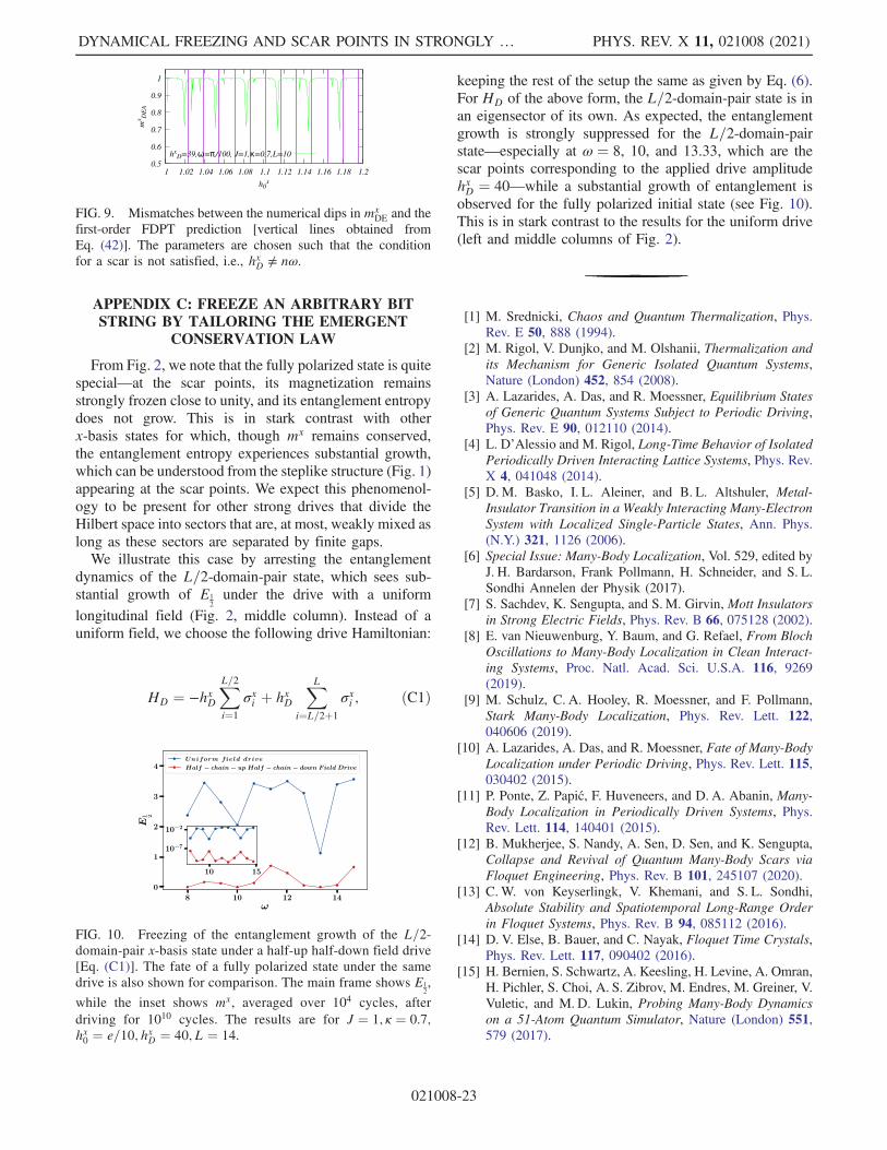
APPENDIX C: FREEZE AN ARBITRARY BITSTRING BY TAILORING THE EMERGENT

CONSERVATION LAW

From Fig. 2, we note that the fully polarized state is quitespecial—at the scar points, its magnetization remainsstrongly frozen close to unity, and its entanglement entropydoes not grow. This is in stark contrast with otherx-basis states for which, though mx remains conserved,the entanglement entropy experiences substantial growth,which can be understood from the steplike structure (Fig. 1)appearing at the scar points. We expect this phenomenol-ogy to be present for other strong drives that divide theHilbert space into sectors that are, at most, weakly mixed aslong as these sectors are separated by finite gaps.We illustrate this case by arresting the entanglement

dynamics of the L=2-domain-pair state, which sees sub-stantial growth of E1

2under the drive with a uniform

longitudinal field (Fig. 2, middle column). Instead of auniform field, we choose the following drive Hamiltonian:

HD ¼ −hxDXL=2i¼1

σxi þ hxDXL

i¼L=2þ1

σxi ; ðC1Þ

keeping the rest of the setup the same as given by Eq. (6).For HD of the above form, the L=2-domain-pair state is inan eigensector of its own. As expected, the entanglementgrowth is strongly suppressed for the L=2-domain-pairstate—especially at ω ¼ 8, 10, and 13.33, which are thescar points corresponding to the applied drive amplitudehxD ¼ 40—while a substantial growth of entanglement isobserved for the fully polarized initial state (see Fig. 10).This is in stark contrast to the results for the uniform drive(left and middle columns of Fig. 2).

[1] M. Srednicki, Chaos and Quantum Thermalization, Phys.Rev. E 50, 888 (1994).

[2] M. Rigol, V. Dunjko, and M. Olshanii, Thermalization andits Mechanism for Generic Isolated Quantum Systems,Nature (London) 452, 854 (2008).

[3] A. Lazarides, A. Das, and R. Moessner, Equilibrium Statesof Generic Quantum Systems Subject to Periodic Driving,Phys. Rev. E 90, 012110 (2014).

[4] L. D’Alessio and M. Rigol, Long-Time Behavior of IsolatedPeriodically Driven Interacting Lattice Systems, Phys. Rev.X 4, 041048 (2014).

[5] D. M. Basko, I. L. Aleiner, and B. L. Altshuler, Metal-Insulator Transition in a Weakly Interacting Many-ElectronSystem with Localized Single-Particle States, Ann. Phys.(N.Y.) 321, 1126 (2006).

[6] Special Issue: Many-Body Localization, Vol. 529, edited byJ. H. Bardarson, Frank Pollmann, H. Schneider, and S. L.Sondhi Annelen der Physik (2017).

[7] S. Sachdev, K. Sengupta, and S. M. Girvin, Mott Insulatorsin Strong Electric Fields, Phys. Rev. B 66, 075128 (2002).

[8] E. van Nieuwenburg, Y. Baum, and G. Refael, From BlochOscillations to Many-Body Localization in Clean Interact-ing Systems, Proc. Natl. Acad. Sci. U.S.A. 116, 9269(2019).

[9] M. Schulz, C. A. Hooley, R. Moessner, and F. Pollmann,Stark Many-Body Localization, Phys. Rev. Lett. 122,040606 (2019).

[10] A. Lazarides, A. Das, and R. Moessner, Fate of Many-BodyLocalization under Periodic Driving, Phys. Rev. Lett. 115,030402 (2015).

[11] P. Ponte, Z. Papić, F. Huveneers, and D. A. Abanin, Many-Body Localization in Periodically Driven Systems, Phys.Rev. Lett. 114, 140401 (2015).

[12] B. Mukherjee, S. Nandy, A. Sen, D. Sen, and K. Sengupta,Collapse and Revival of Quantum Many-Body Scars viaFloquet Engineering, Phys. Rev. B 101, 245107 (2020).

[13] C. W. von Keyserlingk, V. Khemani, and S. L. Sondhi,Absolute Stability and Spatiotemporal Long-Range Orderin Floquet Systems, Phys. Rev. B 94, 085112 (2016).

[14] D. V. Else, B. Bauer, and C. Nayak, Floquet Time Crystals,Phys. Rev. Lett. 117, 090402 (2016).

[15] H. Bernien, S. Schwartz, A. Keesling, H. Levine, A. Omran,H. Pichler, S. Choi, A. S. Zibrov, M. Endres, M. Greiner, V.Vuletic, and M. D. Lukin, Probing Many-Body Dynamicson a 51-Atom Quantum Simulator, Nature (London) 551,579 (2017).

FIG. 10. Freezing of the entanglement growth of the L=2-domain-pair x-basis state under a half-up half-down field drive[Eq. (C1)]. The fate of a fully polarized state under the samedrive is also shown for comparison. The main frame shows E1

2,

while the inset shows mx, averaged over 104 cycles, afterdriving for 1010 cycles. The results are for J ¼ 1; κ ¼ 0.7;hx0 ¼ e=10; hxD ¼ 40; L ¼ 14.

FIG. 9. Mismatches between the numerical dips in mxDE and the

first-order FDPT prediction [vertical lines obtained fromEq. (42)]. The parameters are chosen such that the conditionfor a scar is not satisfied, i.e., hxD ≠ nω.

DYNAMICAL FREEZING AND SCAR POINTS IN STRONGLY … PHYS. REV. X 11, 021008 (2021)

021008-23

[16] C. J. Turner, A. A. Michailidis, D. A. Abanin, M. Serbyn,and Z. Papic, Weak Ergodicity Breaking from QuantumMany-Body Scars, Nat. Phys. 14, 745 (2018).

[17] N. Shiraishi and T. Mori, Systematic Construction ofCounterexamples to the Eigenstate Thermalization Hypoth-esis, Phys. Rev. Lett. 119, 030601 (2017).

[18] C. J. Turner, A. A. Michailidis, D. A. Abanin, M. Serbyn,and Z. Papić, Quantum Scarred Eigenstates in a RydbergAtom Chain: Entanglement, Breakdown of Thermalization,and Stability to Perturbations, Phys. Rev. B 98, 155134(2018).

[19] V. Khemani, C. R. Laumann, and A. Chandran, Signaturesof Integrability in the Dynamics of Rydberg-BlockadedChains, Phys. Rev. B 99, 161101(R) (2019).

[20] W.W.I Ho, S. Choi, H. Pichler, and M. D. Lukin, PeriodicOrbits, Entanglement, and Quantum Many-Body Scars inConstrained Models: Matrix Product State Approach, Phys.Rev. Lett. 122, 040603 (2019).

[21] S. Choi, C. J. Turner, H. Pichler, W.W. Ho, A. A.Michailidis, Z. Papić, M. Serbyn, M. D. Lukin, and D. A.Abanin, Emergent SU(2) Dynamics and Perfect QuantumMany-Body Scars, Phys. Rev. Lett. 122, 220603 (2019).

[22] S. Moudgalya, N. Regnault, and B. A. Bernevig, Entangle-ment of Exact Excited States of Affleck-Kennedy-Lieb-Tasaki Models: Exact Results, Many-Body Scars,and Violation of the Strong Eigenstate ThermalizationHypothesis, Phys. Rev. B 98, 235156 (2018).

[23] V. Khemani, M. Hermele, and R. Nandkishore, Localizationfrom Hilbert Space Shattering: From Theory to PhysicalRealizations, Phys. Rev. B 101, 174204 (2020).

[24] S. Moudgalya, S. Rachel, B. A. Bernevig, and N. Regnault,Exact Excited States of Nonintegrable Models, Phys. Rev. B98, 235155 (2018).

[25] R. Mondaini, K. Mallayya, L. F. Santos, and M. Rigol,Comment on Systematic Construction of Counterexamplesto the Eigenstate Thermalization Hypothesis, Phys. Rev.Lett. 121, 038901 (2018).

[26] L. D’Alessio and A. Polkovnikov, Many-Body EnergyLocalization Transition in Periodically Driven Systems,Ann. Phys. (N.Y.) 333, 19 (2013).

[27] M. Bukov, M. Heyl, D. A. Huse, and A. Polkovnikov,Heating and Many-Body Resonances in a PeriodicallyDriven Two-Band System, Phys. Rev. B 93, 155132(2016).

[28] M. Bukov, L. D’Alessio, and A. Polkovnikov, UniversalHigh-Frequency Behavior of Periodically Driven Systems:From Dynamical Stabilization to Floquet Engineering,Adv. Phys. 64, 139 (2015).

[29] A. Agarwala and D. Sen, Effects of Interactions onPeriodically Driven Dynamically Localized Systems, Phys.Rev. B 95, 014305 (2017).

[30] S. Dasgupta, U. Bhattacharya, and A. Dutta, Phase Tran-sition in the Periodically Pulsed Dicke Model, Phys. Rev. E91, 052129 (2015).

[31] P. Bordia, H. Lüschen, U. Schneider, M. Knap, and I. Bloch,Thermalization and Its Mechanism for Generic IsolatedQuantum Systems, Nat. Phys. 13, 460 (2017).

[32] S. Pal, N. Nishad, T. S. Mahesh, and G. J. Sreejith, Tem-poral Order in Periodically Driven Spins in Star-ShapedClusters, Phys. Rev. Lett. 120, 180602 (2018).

[33] T. Qin and W. Hofstetter, Nonequilibrium Steady States andResonant Tunneling in Time-Periodically Driven Systemswith Interactions, Phys. Rev. B 97, 125115 (2018).

[34] K. Seetharam, P. Titum, M. Kolodrubetz, and G. Refael,Absence of Thermalization in Finite Isolated InteractingFloquet Systems, Phys. Rev. B 97, 014311 (2018).

[35] T. Prosen, Time Evolution of a Quantum Many-BodySystem: Transition from Integrability to Ergodicity in theThermodynamic Limit, Phys. Rev. Lett. 80, 1808 (1998).

[36] T. Prosen, General Relation between Quantum Ergodicityand Fidelity of Quantum Dynamics, Phys. Rev. E 65,036208 (2002).

[37] D. J. Luitz, A. Lazarides, and Y. B. Lev, Periodic andQuasiperiodic Revivals in Periodically Driven InteractingQuantum Systems, Phys. Rev. B 97, 020303(R) (2018).

[38] A. Haldar, R. Moessner, and A. Das, Onset of FloquetThermalization, Phys. Rev. B 97, 245122 (2018).

[39] A. Das, Exotic Freezing of Response in a Quantum Many-Body System, Phys. Rev. B 82, 172402 (2010).

[40] S. Bhattacharyya, A. Das, and S. Dasgupta, TransverseIsing Chain under Periodic Instantaneous Quenches:Dynamical Many-Body Freezing and Emergence of SlowSolitary Oscillations, Phys. Rev. B 86, 054410 (2012).

[41] S. S. Hegde, H. Katiyar, T. S. Mahesh, and A. Das, Freezinga Quantum Magnet by Repeated Quantum Interference: AnExperimental Realization, Phys. Rev. B 90, 174407 (2014).

[42] S. Mondal, D. Pekker, and K. Sengupta, Dynamics-InducedFreezing of Strongly Correlated Ultracold Bosons, Euro-phys. Lett. 100, 60007 (2012).

[43] A. Russomanno, A. Silva, and G. E. Santoro, LinearResponse as a Singular Limit for a Periodically DrivenClosed Quantum System, J. Stat. Mech. (2013) P09012.

[44] A. Lazarides, A Das, and R Moessner, Periodic Thermo-dynamics of Isolated Systems, Phys. Rev. Lett. 112, 150401(2014).

[45] K. Seetharam, P. Titum, M. Kolodrubetz, and G. Refael,Absence of Thermalization in Finite Isolated InteractingFloquet Systems, Phys. Rev. B 97, 014311 (2018).

[46] M. Rodriguez-Vega, M. Lentz, and B. Seradjeh, FloquetPerturbation Theory: Formalism and Application to Low-Frequency Limit, New J. Phys. 20, 093022 (2018).

[47] M. Vogl, P. Laurell, A. D. Barr, and G. A. Fiete, FlowEquation Approach to Periodically Driven Quantum Sys-tems, Phys. Rev. X 9, 021037 (2019).

[48] M. Vogl, M. Rodriguez-Vega, and G. A. Fiete, EffectiveFloquet Hamiltonian in the Low-Frequency Regime, Phys.Rev. B 101, 024303 (2020).

[49] M. Srednicki, Does Quantum Chaos Explain QuantumStatistical Mechanics?, arXiv:cond-mat/9410046v2.

[50] M. Rigol, V. Dunjko, V. Yurovsky, and M. Olshanii,Relaxation in a Completely Integrable Many-Body Quan-tum System: An Ab Initio Study of the Dynamics of theHighly Excited States of 1D Lattice Hard-Core Bosons,Phys. Rev. Lett. 98, 050405 (2007).

[51] A. C. Cassidy, C. W. Clark, and M. Rigol, GeneralizedThermalization in an Integrable Lattice System, Phys. Rev.Lett. 106, 140405 (2011).

[52] P. Reimann, Foundation of Statistical Mechanics underExperimentally Realistic Conditions, Phys. Rev. Lett. 101,190403 (2008).

HALDAR, SEN, MOESSNER, and DAS PHYS. REV. X 11, 021008 (2021)

021008-24

[53] A. Eckardt and E. Anisimovas, High-Frequency Approxi-mation for Periodically Driven Quantum Systems from aFloquet-Space Perspective, New J. Phys. 17, 093039(2015).

[54] A. Soori and D. Sen, Nonadiabatic Charge Pumping byOscillating Potentials in One Dimension: Results forInfinite System and Finite Ring, Phys. Rev. B 82, 115432(2010).

[55] J. Zhang, P.W. Hess, A. Kuprianidis, P. Becker, A. Lee,J. Smith, G. Pagano, I.-D. Potirniche, A. C. Potter, A.Vishwanath, N. Y. Yao, and C Monroe, Observation of aDiscrete Time Crystal, Nature (London) 543, 217 (2017).

[56] J. Rovny, R. L. Blum, and S. E. Barrett, Observationof Discrete-Time-Crystal Signatures in an Ordered Dipo-lar Many-Body System, Phys. Rev. Lett. 120, 180603(2018).

[57] A. Das and R. Moessner, Switching the Anomalous DCResponse of an AC-driven Quantum Many-Body System,arXiv:1208.0217.

[58] M. Bukov, Ph.D. thesis, Boston University, 2016, https://mgbukov.github.io/files/Floquet_thesis.pdf.

[59] P. Weinberg and M. Bukov, QuSpin: A Python Package forDynamics and Exact Diagonalisation of Quantum ManyBody Systems Part I: Spin Chains, SciPost Phys. 2, 003(2017).

[60] P. Weinberg and M.Bukov, QuSpin: A Python Package forDynamics and Exact Diagonalisation of Quantum ManyBody Systems. Part II: Bosons, Fermions and Higher Spins,SciPost Phys. 7, 20 (2019).

[61] D. J. Luitz, R. Moessner, S. L. Sondhi, and V. Khemani,Prethermalization without Temperature, Phys. Rev. X 10,021046 (2020).

DYNAMICAL FREEZING AND SCAR POINTS IN STRONGLY … PHYS. REV. X 11, 021008 (2021)

021008-25