Embed Size (px)
Citation preview
PHYSICAL REVIEW B 98, 235156 (2018)Editors’ Suggestion
Entanglement of exact excited states of Affleck-Kennedy-Lieb-Tasaki models: Exact results,many-body scars, and violation of the strong eigenstate thermalization hypothesis
Sanjay Moudgalya,1 Nicolas Regnault,2 and B. Andrei Bernevig1,3,4,5,6,2
1Department of Physics, Princeton University, Princeton, New Jersey 08544, USA2Laboratoire Pierre Aigrain, Ecole normale supérieure, PSL University, Sorbonne Université,Université Paris Diderot, Sorbonne Paris Cité, CNRS, 24 rue Lhomond, 75005 Paris France
3Dahlem Center for Complex Quantum Systems and Fachbereich Physik, Freie Universitat Berlin, Arnimallee 14, 14195 Berlin, Germany4Max Planck Institute of Microstructure Physics, 06120 Halle, Germany
5Donostia International Physics Center, P. Manuel de Lardizabal 4, 20018 Donostia-San Sebastián, Spain6Sorbonne Universités, UPMC Univ Paris 06, UMR 7589, LPTHE, F-75005, Paris, France
(Received 7 July 2018; published 27 December 2018)
We obtain multiple exact results on the entanglement of the exact excited states of nonintegrable models weintroduced in Phys. Rev. B 98, 235155 (2018). We first discuss a general formalism to analytically computethe entanglement spectra of exact excited states using matrix product states and matrix product operators andillustrate the method by reproducing a general result on single-mode excitations. We then apply this technique toanalytically obtain the entanglement spectra of the infinite tower of states of the spin-S AKLT models in the zeroand finite energy density limits. We show that in the zero energy density limit, the entanglement spectra of thetower of states are multiple shifted copies of the ground-state entanglement spectrum in the thermodynamic limit.We show that such a resemblance is destroyed at any nonzero energy density. Furthermore, the entanglemententropy S of the states of the tower that are in the bulk of the spectrum is subthermal S ∝ log L, as opposed to avolume law S ∝ L, thus indicating a violation of the strong eigenstate thermalization hypothesis (ETH). Thesestates are examples of what are now called many-body scars. Finally, we analytically study the finite-size effectsand symmetry-protected degeneracies in the entanglement spectra of the excited states, extending the existingtheory.
DOI: 10.1103/PhysRevB.98.235156
I. INTRODUCTION
Nonintegrable translation invariant models have been ofgreat interest recently. Such models have very few conservedquantities and show various interesting dynamical phenom-ena, including thermalization [1] and, upon the introduc-tion of disorder or quasiperiodicity, many-body localization[2–4]. Since dynamics depends on the properties of all theeigenstates, highly excited states of nonintegrable modelshave been extensively studied in various models in one andtwo dimensions [1,5–14]. Particularly, the eigenstates in thebulk of the spectrum of several nonintegrable models areexpected to satisfy the eigenstate thermalization hypothesis(ETH) [1,15,16], with the notable exception of many-bodylocalized (MBL) systems [5,11,17]. While several analyticalresults on the entanglement structure of highly excited statesin generic models have been obtained [18–21], exactly solv-able examples are desired.
The entanglement structure of low-energy excitations inintegrable and nonintegrable models has been studied analyti-cally and numerically in detail [22–29], particularly using thelanguage of matrix product states (MPS) [30,31]. Similar tothe ground states of gapped Hamiltonians [32], low-energyexcited states of gapped Hamiltonians are, in principle, alsocaptured by this MPS framework [22]. However, even withinsingle-mode excitations, the lack of explicit examples hashindered a study of their entanglement in more detail; for
example, the general nature of finite-size corrections to theentanglement spectra is unknown. Beyond low-energy exci-tations, the structure of excited states has been studied inthe MBL regime, where all the eigenstates exhibit area-lawentanglement [17], and consequently have an efficient MPSrepresentation [33–35]. In the thermal regime, however, verylittle is analytically known about the kind of excited states thatcan exist in the bulk of the spectrum of generic nonintegrablemodels [36–41]. For example, can certain highly excited statesof thermal nonintegrable models have an exact or approximatematrix product structure with a finite or low bond dimensionin the thermodynamic limit?
Recently, a tower of exact excited states were analyticallyobtained by us in a family of nonintegrable models, the spin-SAKLT models [42]. The entanglement of the ground states ofthe spin-S AKLT models and their generalizations has beenextensively studied in the literature [43–53]. Being the firstfew known examples of exact eigenstates of nonintegrablemodels, we propose to use the excited states of these modelsto test conjectures on eigenstates that exist in the literature.We recover the general entanglement spectra of single-modeexcitations, earlier obtained on general grounds [22,23]. Wealso derive the entanglement spectrum of an entire towerof exact states, thus generalizing the single-mode results tothese set of states. The tower of states have an interestingentanglement structure in that the zero energy density statesentanglement spectra is composed of shifted copies of the
2469-9950/2018/98(23)/235156(43) 235156-1 ©2018 American Physical Society
MOUDGALYA, REGNAULT, AND BERNEVIG PHYSICAL REVIEW B 98, 235156 (2018)
ground-state entanglement spectrum. This structure general-izes the earlier result obtained on the entanglement spectra ofSMA excitations. We find that the finite energy density statesin the tower have a subthermal entanglement entropy scalingin spite of the fact that they appear to be in the bulk of thespectrum [42]. More precisely, the entanglement entropy Sfor these states scales as S ∝ ln L, where L is the subsystemsize. This indicates a violation of the strong ETH [54,55],which states that all the eigenstates in the bulk of the spectrumof a nonintegrable model in a given quantum number sectorare thermal, i.e., their entanglement entropy scales with thevolume of the subsystem (S ∝ L).
This paper is organized as follows. We begin by reviewingthe tools we use to compute the entanglement spectrum, i.e.,matrix product states (MPS) and their properties in Sec. II andmatrix product operators (MPO) in Sec. IV. In these sections,we provide some examples for the AKLT models. Readersfamiliar with these approaches can directly proceed to Sec. V,where we discuss the structure and properties of states that arecreated by the action of an operator (MPO) on the ground state(MPS). From Sec. VI, we move on to the main results andderive the entanglement spectra of single-mode excitations,focusing on the AKLT Arovas states and spin-2S magnons. InSecs. VII and VIII, we consider states beyond single-modeexcitations. We compute the entanglement spectrum of thetower of states in spin-S AKLT models, where we work inthe zero energy density and finite energy density regimesseparately. Further, in Sec. IX, we discuss the violation of theeigenstate thermalization hypothesis and then show numericalresults away from the AKLT point. In Secs. X and XI, we re-view symmetries and their effects on the entanglement spectraof the ground states, and discuss symmetry-protected exactdegeneracies and finite-size splittings in the entanglementspectra of the excited states. We close with conclusions andoutlook in Sec. XII.
II. MATRIX PRODUCT STATES
In this section, we provide a basic introduction to thematrix product states (MPS) and their properties. We invitereaders not familiar with MPS to read numerous reviews andlecture notes in the literature [30,31,56,57].
A. Definition and properties
We consider a spin-S chain with L sites. A simple many-body basis for the system is made of the product states|m1m2 . . . mL〉, where mi = −S,−S + 1, . . . , S − 1, S is theprojection along the z axis of the spin at site i. Any wavefunction of the many-body Hilbert space can be decomposedas
|ψ〉 =∑
{m1,m2,...,mL}cm1m2...mL
|m1m2 . . . mL〉. (1)
In all generality, the coefficients cm1,m2...mLcan always be
written as an MPS [32], i.e.,
cm1,m2...mL= [
blA
TA
[m1]1 A
[m2]2 . . . A
[mL]L br
A
]. (2)
The state |ψ〉 then reads
|ψ〉 =∑
{m1m2...mL}
[bl
A
TA
[m1]1 . . . A
[mL]L br
A
]|m1 . . . mL〉. (3)
In Eqs. (2) and (3), A[m1]1 , . . . , A
[mL−1]L−1 and A
[mL]L are χ × χ
matrices over an auxiliary space. χ is the bond dimensionof the MPS and the corresponding indices are the ancilla. bl
A
and brA are χ -dimensional left and right boundary vectors that
determine the boundary conditions for the wave function. The{[mi]} are called the physical indices and can take d = 2S + 1values (d is the physical dimension, i.e., the dimension of thelocal physical Hilbert space on site i). In a compact notation,we can think of the Ai’s as d × χ × χ tensors.
An MPS representation is particularly powerful if the ma-trices A
[mi ]i are site-independent, i.e., A[mi ]
i = A[mi ]. Typically,translation invariant systems admit such a site independentMPS. Many computations involving an MPS can then besimplified once we introduce the transfer matrix
E =∑m
A[m]∗ ⊗ A[m], (4)
where ∗ denotes complex conjugation and the ⊗ is over theancilla. The transfer matrix is thus a χ × χ × χ × χ tensorthat can also be viewed as χ2 × χ2 matrix by groupingthe left and right ancilla of the two MPS copies together.The simplification provided by the MPS description can beillustrated by computing the norm 〈ψ |ψ〉 of the state |ψ〉,
〈ψ |ψ〉 = blT
EELbrE, (5)
where blE and br
E are the left and right boundary vectors of thetransfer matrix defined as
blE = (
blA
∗ ⊗ blA
), br
E = (br
A∗ ⊗ br
A
). (6)
An MPS representation is said to be in a left (right) canonicalform if the largest left (right) eigenvalue of the transfer matrixE is unique, is equal to 1 (this can always be obtained byrescaling the B’s) and most importantly the corresponding left(right) eigenvector is the identity χ × χ matrix [57]. Thus, fora right canonical MPS,∑
γ,ε
Eαβ,γ εδγ,ε = δαβ, (7)
where δ denotes the Kronecker delta function. However, ingeneral, an MPS cannot be in both a left and right canonicalform simultaneously.
Another useful construction with an MPS is the general-ized transfer matrix EO ,
EO =∑n,m
A[m]∗ ⊗ OmnA[n]. (8)
Here, O is any single-site operator with matrix elements〈m|O|n〉 = Omn. EO is useful when computing the expecta-tion value of an operator O acting on a site i, where
〈ψ |Oi |ψ〉 = blE
TEi−1EOEL−ibr
E. (9)
Similarly, assuming i < j , the two-point function associatedwith O reads
〈ψ |OiOj |ψ〉 = blE
TEi−1EOEj−i−1EOEL−j br
E. (10)
235156-2

ENTANGLEMENT OF EXACT EXCITED STATES OF … PHYSICAL REVIEW B 98, 235156 (2018)
Using Eqs. (9) and (10) for large L, the correlation length ξ ofthe MPS defined using
〈OiOj 〉 − 〈Oi〉〈Oj 〉 ∼ exp
(−|i − j |
ξ
)(11)
is given by
ξ = − 1
ln |ε2| , (12)
where ε2 is the second largest eigenvalue of the transfermatrix [31]. Note that −1/ ln |ε2| is an upper bound for ξ
that is saturated unless O has a special structure. Thus, ifthe spectrum of the transfer matrix is gapless, the state hasan infinite correlation length. Note that a finite correlationlength for an MPS in a canonical form guarantees that thewave function is normalized in the thermodynamic limit.
B. Entanglement spectrum and MPS
The MPS representation of any wave function encodes theentanglement structure of the wave function. For any state |ψ〉with a number L of spin-S’, a bipartition into two contiguousregions A and B with an LA number of spins in region A andan LB number of spins in region B (LA + LB = L) is definedas
|ψ〉 =χ∑
α=1
|ψA〉α ⊗ |ψB〉α, (13)
where |ψA〉α and |ψB〉α are many-body states belonging to thephysical Hilbert spaces of subsystems A and B respectively.Using the MPS representation of |ψ〉 (3), if the region A isdefined as the set of sites {1, 2, . . . , LA} and the region B as{LA + 1, LA + 2, . . . , L}, the bipartition can be written using
|ψA〉α =∑
{mi },i∈A
[bl
A
T∏l∈A
A[ml ]l
]α
|{mi}〉,
|ψB〉α =∑
{mi },i∈B
[∏l∈B
A[ml ]l br
A
]α
|{mi}〉. (14)
Note that {|ψA〉α} and {|ψB〉α} form complete but not nec-essarily orthonormal bases on the subsystems A and B, re-spectively. The reduced density matrix with respect to such abipartition is constructed as ρA = TrB|ψ〉〈ψ |. The eigenvaluespectrum of − ln ρA is the entanglement spectrum and S ≡−TrA (ρA ln ρA) is the von Neumann entanglement entropy.An alternate way to obtain ρA that is useful for MPS is throughthe definition of Gram matrices L and R,
Lαβ = α〈ψA|ψA〉β, Rαβ = α〈ψB|ψB〉β. (15)
Up to an overall normalization factor, the reduced densitymatrix can be expressed in terms of these Gram matrices as[58]
ρA =√LRT
√L, (16)
where√L is well-defined since Gram matrices are positive
semidefinite. The Gram matrices L and R can be expressed interms of the MPS transfer matrix E of Eq. (4) as
L = (ET )LAblE, R = ELBbr
E. (17)
In Eq. (17), E is viewed as a χ × χ × χ × χ tensor, blE and
brE as χ × χ matrices. Consequently, L and R are χ × χ
matrices. Note that ρA in Eq. (16) has the same spectrum asthe matrix
ρred = LRT . (18)
Since we are only interested in the spectrum of ρA in thisarticle, we refer to ρred to be the reduced density matrix ofthe system even though it is not guaranteed to be Hermitian.Assuming that the eigenvalue of unit magnitude of the transfermatrix is nondegenerate (i.e., ln |ε2| �= 0), if LA and LB arelarge, (ET )
LA and ELB project onto eL and eR , the left andright eigenvectors corresponding to the largest eigenvalue ofE. Thus
L = eL
(eTLbl
E
), R = eR
(eTRbr
E
). (19)
The density matrix thus reads, up to an overall constant [equalto (eT
LblE )(eT
RbrE )],
ρred = eLeTR. (20)
One should note that the construction of an MPS for agiven state is not unique. Indeed, MPS matrices and boundaryvectors redefined as
A[m] = GA[m]G−1, blA = G−1T
blA, br
A = GbrA (21)
represent the same wave function. When constructed in acanonical form, the bipartition Eq. (13) is the same as aSchmidt decomposition [57] of the state |ψ〉 with respect tosubregions A and B, defined as
|ψ〉 =χs∑
α=1
λα
∣∣ψsA⟩α
∣∣ψsB⟩α, (22)
where {|ψsA〉
α} and {|ψs
B〉α} are sets of orthonormal vectors on
the subsystems A and B respectively and {λα} are referredto as the Schmidt values and χs is the number of nonzeroSchmidt values (Schmidt rank). The bond dimension χ of theMPS constructed in the canonical form is the Schmidt rank χs
of the wave function |ψ〉. Thus we refer to χs as the optimumbond dimension for an MPS representation of state |ψ〉. Theentanglement entropy then satisfies
S = −χs∑
α=1
λ2α ln λ2
α � ln χs. (23)
The entanglement entropy of an MPS about a given cut is thusupper-bounded by ln χs . Since the Schmidt decompositionis the optimal bipartition of the system, χ � χs and henceS � ln χ .
III. MPS AND THE AKLT MODELS
In this section, we provide a few examples of MPS basedon the AKLT models.
A. Ground state of the spin-1 AKLT model
We first focus on the ground state of the spin-1 AKLTmodel with open boundary conditions (OBC) [59], one of thefirst examples of an MPS [60]. The state with L spin-1’s canbe thought to be composed of two spin-1/2 Schwinger bosons,
235156-3
MOUDGALYA, REGNAULT, AND BERNEVIG PHYSICAL REVIEW B 98, 235156 (2018)
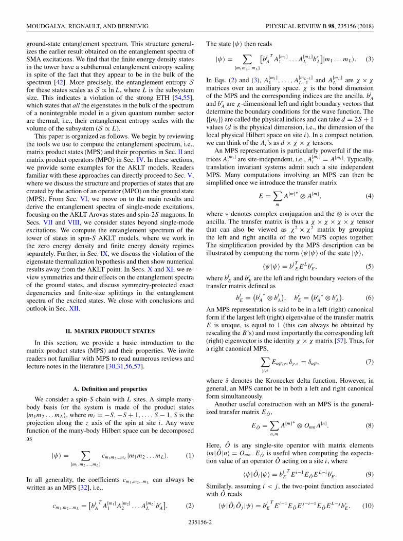
FIG. 1. Ground state of the spin-1 AKLT model with openboundary conditions. Big and small circles represent physical spin-1and spin-1/2 Schwinger bosons, respectively. The lines representsinglets between spin-1/2. The two edge spin-1/2’s are free.
each in a singlet configuration with the spin-1/2 Schwingerboson of the left and right nearest neighbor spin-1s. Thus thereare dangling spin-1/2’s on each edge of the chain. A cartoonpicture of this state is shown in Fig. 1. For a more detaileddiscussion of the model, we refer the reader to Ref. [42].
The two spin-1/2 Schwinger bosons within a spin-1 (seeFig. 1) form a virtual Hilbert space that corresponds to theauxillary space of the MPS. The normalized wave functioncan be written as a matrix product state with physical dimen-sion d = 3 (the Hilbert space dimension of the physical spin-1) and a bond dimension χ = 2 (the Hilbert space dimensionof the spin-1/2 Schwinger boson) [30]. The derivation of theMPS representation for this state is shown in Appendix A. Thed normalized χ × χ matrices for the AKLT ground state are[see Eq. (A17)]
A[1] =√
2
3
(0 10 0
),
A[0] = 1√3
(−1 00 1
), (24)
A[−1] =√
2
3
(0 0
−1 0
),
corresponding to Sz = 1, 0,−1 of the physical spin-1, respec-tively.
Using the matrices of Eq. (24), the AKLT ground-statetransfer matrix can be computed to be
E =
⎛⎜⎜⎝13 0 0 2
30 − 1
3 0 00 0 − 1
3 023 0 0 1
3
⎞⎟⎟⎠, (25)
where the left and right indices of the transfer matrix aregrouped together. The eigenvalues of this transfer matrix are(1,− 1
3 ,− 13 ,− 1
3 ). Since the largest eigenvalue is nondegener-ate, using Eq. (12) the AKLT ground state is a finitely corre-lated state with correlation length ξ = 1/ ln(3). The boundaryvectors of Eq. (3) for the AKLT ground state correspond to thefree spin-1/2’s on the left and right edges of an open spin-1chain, shown in Fig. 1. With both edge spins set to Sz = +1/2the boundary vectors are [see Eq. (A17)]
blA =
(10
), br
A =(
01
). (26)
The Gram matrices L and R for the AKLT ground state are theleft and right eigenvectors of E corresponding to eigenvalue 1,L = R = 1√
212×2. Using Eq. (18), the reduced density matrix
is ρred = 1212×2 and the entanglement entropy is S = ln 2,
corresponding to a free spin-1/2 dangling spin.
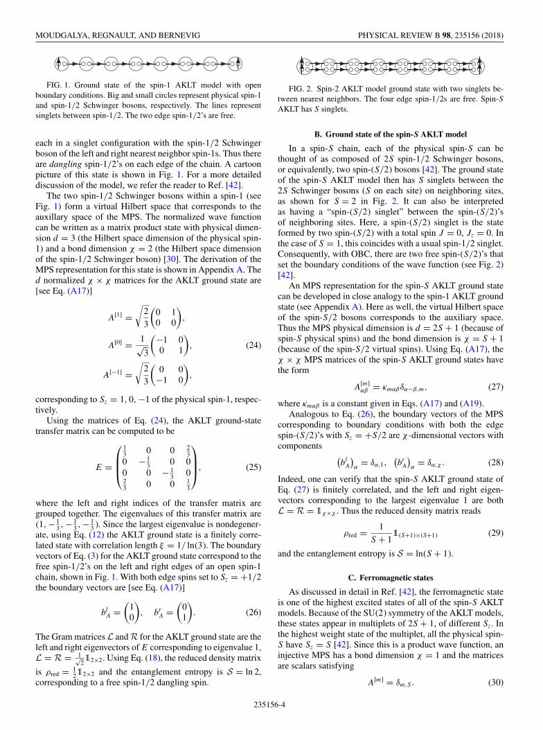
FIG. 2. Spin-2 AKLT model ground state with two singlets be-tween nearest neighbors. The four edge spin-1/2s are free. Spin-SAKLT has S singlets.
B. Ground state of the spin-S AKLT model
In a spin-S chain, each of the physical spin-S can bethought of as composed of 2S spin-1/2 Schwinger bosons,or equivalently, two spin-(S/2) bosons [42]. The ground stateof the spin-S AKLT model then has S singlets between the2S Schwinger bosons (S on each site) on neighboring sites,as shown for S = 2 in Fig. 2. It can also be interpretedas having a “spin-(S/2) singlet” between the spin-(S/2)’sof neighboring sites. Here, a spin-(S/2) singlet is the stateformed by two spin-(S/2) with a total spin J = 0, Jz = 0. Inthe case of S = 1, this coincides with a usual spin-1/2 singlet.Consequently, with OBC, there are two free spin-(S/2)’s thatset the boundary conditions of the wave function (see Fig. 2)[42].
An MPS representation for the spin-S AKLT ground statecan be developed in close analogy to the spin-1 AKLT groundstate (see Appendix A). Here as well, the virtual Hilbert spaceof the spin-S/2 bosons corresponds to the auxiliary space.Thus the MPS physical dimension is d = 2S + 1 (because ofspin-S physical spins) and the bond dimension is χ = S + 1(because of the spin-S/2 virtual spins). Using Eq. (A17), theχ × χ MPS matrices of the spin-S AKLT ground states havethe form
A[m]αβ = κmαβδα−β,m, (27)
where κmαβ is a constant given in Eqs. (A17) and (A19).Analogous to Eq. (26), the boundary vectors of the MPS
corresponding to boundary conditions with both the edgespin-(S/2)’s with Sz = +S/2 are χ -dimensional vectors withcomponents (
blA
)α
= δα,1,(br
A
)α
= δα,χ . (28)
Indeed, one can verify that the spin-S AKLT ground state ofEq. (27) is finitely correlated, and the left and right eigen-vectors corresponding to the largest eigenvalue 1 are bothL = R = 1χ×χ . Thus the reduced density matrix reads
ρred = 1
S + 11(S+1)×(S+1) (29)
and the entanglement entropy is S = ln(S + 1).
C. Ferromagnetic states
As discussed in detail in Ref. [42], the ferromagnetic stateis one of the highest excited states of all of the spin-S AKLTmodels. Because of the SU(2) symmetry of the AKLT models,these states appear in multiplets of 2S + 1, of different Sz. Inthe highest weight state of the multiplet, all the physical spin-S have Sz = S [42]. Since this is a product wave function, aninjective MPS has a bond dimension χ = 1 and the matricesare scalars satisfying
A[m] = δm,S. (30)
235156-4
ENTANGLEMENT OF EXACT EXCITED STATES OF … PHYSICAL REVIEW B 98, 235156 (2018)
The boundary vectors are just 1 and this trivial MPS leads toa trivial transfer matrix, which is a scalar 1. Thus ρ = 1 andS = 0.
IV. MATRIX PRODUCT OPERATORS
In this section, we briefly review matrix product operators(MPO) and provide some examples relevant to the AKLTmodels. A comprehensive discussion of MPOs can be foundin existing literature [30,56,61–63].
A. Definition and properties
Since the exact excited states derived in Ref. [42] areexpressed in terms of operators on the ground state or thehighest excited state, it is crucial to understand how to applythese operators on an MPS. An MPO representation of anoperator O is defined as
O =∑
{sn},{tn}
[bl
M
TM
[s1t1]1 M
[s2t2]2 . . . M
[sLtL]L br
M
]|{sn}〉〈{tn}|.
(31)
In Eq. (31), the operator O is written in terms of L χm × χm
matrices with elements expressed as d × d matrices acting onthe physical indices. χm is referred to as the bond dimension ofthe MPO and the corresponding vector space is the auxiliaryspace. O can compactly be represented as a χm × χm × d × d
tensor Mi with two physical indices ({[si], [ti]} and two auxil-iary indices. bl
M and brM are the boundary vectors of the MPO
in the operator auxiliary space.Similar to an MPS, the construction of an MPO for a given
operator is not unique. We now describe a method to constructan MPO for an operator O. The particular MPO constructionwe describe here relies on a generalized version of a finitestate automation (FSA) [30,64,65]. An FSA is a system witha finite set of “states” and a set of rules for transition betweenthe states at each iteration. In such a setup, each state maps toa unique state after an iteration. When the states of the FSAare viewed as basis elements of a vector space, each state isdenoted as a vector and the transition between the states isdescribed by a square matrix. For example, we consider anFSA with two states |R〉 and |F 〉, that are denoted as
|R〉 =(
10
), |F 〉 =
(01
). (32)
If at each iteration, |R〉 and |F 〉 are interchanged, the transi-tion matrix T is
T =(
0 11 0
). (33)
In principle, these transition matrices could vary from aniteration to the next.
To exemplify the construction of an MPO, we start with asimple example:
O =L∑
j=1
eikj Cj , (34)
where eikj Cj can be written in the physical Hilbert space as
eikj Cj ≡ eik1 ⊗ · · · ⊗ eik1︸ ︷︷ ︸j−1 times
⊗ eikC ⊗ 1 ⊗ · · · ⊗ 1︸ ︷︷ ︸L−j times
, (35)
such that the index j does not explicitly appear in any ofthe operators. Consider an FSA that iterates L times andconstructs the operator O by appending a physical operator(either 1 or C) at each iteration to a string of operators. If|Sn〉 is the state of the FSA at the nth iteration, the appendedphysical operator is the matrix element 〈Sn|Tn|Sn+1〉 whereTn is the transition matrix at the nth iteration. For example, anFSA that constructs eikjCj of Eq. (35) starts in a state |R〉. Itremains in the state |R〉 for j − 1 iterations with a transitionmatrix
TR =(
eik1 00 0
)(36)
appending an 1 at each step. At the j th iteration, the FSAtransitions to |F 〉 (different from |R〉) with a transition matrixTj ,
Tj =(
0 eikC
0 0
), (37)
thus appending the operator C on site j and remains in |F 〉 inthe rest of L − j iterations with transition matrix
TF =(
0 00 1
). (38)
O is then the sum of operators obtained using an FSA for allj . The sum over operators can be efficiently represented bygeneralizing an FSA to allow for superpositions of FSA stateswith operators as coefficients. For example, we allow for FSAstates such as eik1|R〉 + eikC|F 〉. The transition matrix insuch a generalized FSA is an arbitrary square matrix with op-erators as matrix elements. Indeed, fixing the initial and finalstates of the FSA to be |R〉 and |F 〉, we can construct the op-erator O with a transition matrix Mj on site j with elements:
Mj =(
eik1 eikC
0 1
). (39)
Writing the entire process of the generalized FSA,〈F |∏L
j=1 Mj |R〉, we obtain exactly the representation of
O as an MPO of the form Eq. (31), where the auxiliary spaceis the vector space spanned by states of the generalized FSA.Note that since Mj does not depend on the site index j , wecan omit this index. The left and right boundary vectors bl
M
and brM are the vector representations of the FSA states |R〉
and |F 〉, respectively [Eq. (32)],
blM =
(10
), br
M =(
01
). (40)
The MPO representations of more general operators canbe computed similarly with the introduction of intermediatestates of the generalized FSA. For example, in the construc-tion of the MPO for the operator
O =∑
j
eikj (Wj Xj+1), (41)
one introduces an intermediate state |I1〉 of the generalizedFSA, such that the transition matrix elements at any step read
235156-5
MOUDGALYA, REGNAULT, AND BERNEVIG PHYSICAL REVIEW B 98, 235156 (2018)
〈R|T |I1〉 = eikW and 〈I1|T |F 〉 = X. The MPO for O in theauxiliary dimension thus reads
M =⎛⎝eik1 eikW 0
0 0 X
0 0 1
⎞⎠. (42)
The bond dimension of the MPO χm is the number of statesof the generalized FSA generating it. Since the initial state ofthe FSA is |R〉 and the final state is |F 〉, the components ofthe left and right boundary vectors of an MPO are always(
blM
)α
= δα,1,(br
M
)α
= δα,χm. (43)
Since the flow of an FSA is unidirectional, the MPO isalways an upper triangular matrix in the auxiliary indices.For a translation invariant MPO, any element on the MPOdiagonal appears in the operator as multiple direct productsof the same operator. For example, the MPO
MO =(
W C
0 X
)(44)
represents an operator O defined on a lattice of length L thatreads
O =(
L−1∏i=1
Wi
)CL + C1
(L∏
i=2
Xi
)+ · · · , (45)
which is not a strict local operator unless W and X are propor-tional to 1. Thus, for an operator that is a sum of strictly localterms, the only diagonal element that can appear in the MPOis 1, up to an overall constant (such as eik). Moreover, if thediagonal element in an MPO corresponding to an intermediatestate is 1, the operator O includes a nonlocal term, i.e., a longrange coupling between sites. For example, for the MPO
MO =⎛⎝1 W 0
0 1 X
0 0 1
⎞⎠, (46)
the operator O reads
O =L−1∑i=1
L∑j=i+1
WiXj . (47)
Thus, for operators that are the sum of nontrivial operatorswith a finite support, the only nonvanishing diagonal elementscorrespond to the auxiliary states |R〉 and |F 〉.
B. The AKLT model and MPOs
We now introduce the MPOs for some of the operatorsrequired to build exact excited states of the AKLT model.These will be useful for the study of the entanglement ofthese excited states, introduced in Refs. [42,66]. Whereasthe Arovas A and Arovas B states discussed therein werefor exact eigenstates only for periodic boundary conditions,here we assume open boundary conditions. The motivation forthis assumption is twofold. First, analytic calculations usingMPS and MPOs are greatly simplified with open boundaries.Second, we are interested in the thermodynamic limit or largesystems where the properties of the system are essentiallyindependent of boundary conditions.
We start with the spin-1 AKLT model. The Arovas A statewas introduced in Ref. [66]. The closed-form expression forthe state, up to an overall normalization factor, reads
|A〉 =⎡⎣L−1∑
j=1
(−1)j �Sj · �Sj+1
⎤⎦|G〉, (48)
where |G〉 is the ground state of the spin-1 AKLT model andwe have assumed open boundary conditions. The operator thatappears in the Arovas A state can be written as
OA =∑
j
(−1)j �Sj · �Sj+1
=∑
j
(−1)j(
S+j S−
j+1 + S−j S+
j+1
2+ Sz
jSzj+1
). (49)
By analogy to the MPO of Eq. (42) corresponding to theoperator Eq. (41), the MPO for OA (in the case of openboundary conditions) reads [also see Eq. (B4)]
MA =
⎛⎜⎜⎜⎜⎜⎜⎝−1 − S+√
2− S−√
2−Sz 0
0 0 0 0 S−√2
0 0 0 0 S+√2
0 0 0 0 Sz
0 0 0 0 1
⎞⎟⎟⎟⎟⎟⎟⎠, (50)
where the negative signs appear due to the (−1)j in Eq. (49).Similarly, the Arovas B state, introduced in Ref. [66] is
another exact excited state of the AKLT model [42]. Asmentioned in Ref. [42], its closed-form expression, up to anoverall normalization factor, can be written as
|B〉 = OB |G〉 (51)
with
OB =L−1∑j=2
(−1)j { �Sj−1 · �Sj , �Sj · �Sj+1}, (52)
where we have assumed open boundary conditions. As shownin Eq. (B7) in Appendix B, the MPO for OB can be compactlyexpressed as
MB =
⎛⎜⎜⎝−1 −S 0 00 0 T 00 0 0 S0 0 0 1
⎞⎟⎟⎠, (53)
where
S =(
S+√
2
S−√
2Sz
),
S =(
S−√
2
S+√
2Sz
)T
, (54)
T =
⎛⎜⎜⎝{S−,S+}
2 (S−)2 {S−,Sz}√2
(S+)2 {S+,S−}2
{S+,Sz}√2
{Sz,S+}√2
{Sz,S−}√2
2SzSz
⎞⎟⎟⎠.
The bond dimension of the MPO MB is thus χm = 8.
235156-6

ENTANGLEMENT OF EXACT EXCITED STATES OF … PHYSICAL REVIEW B 98, 235156 (2018)
Another set of excited states for spin-S AKLT modelswas obtained in Ref. [42], i.e., the spin-2S magnons. Theclosed-form expression for the spin-2S magnon state in thespin-S AKLT models, up to an overall normalization factor,reads
|SS2〉 =L∑
j=1
(−1)j (S+j )2S |SG〉, (55)
where |SG〉 is the ground state of the spin-S AKLT model.Unlike the two previous states, |SS2〉 is an exact excited stateirrespective of the boundary conditions [42]. The spin-2S
magnon creation operator thus reads
OSS2 =∑
j
(−1)j (S+j )2S. (56)
Since OSS2 is a sum of single-site operators, by analogy toEqs. (35) and (39), its MPO has χm = 2 and reads
MSS2 =(−1 −(S+)2S
0 1
). (57)
Following the spin-2S magnon in Eq. (56), a tower of statesfrom the ground state to a highest excited state was introducedfor spin-S AKLT models in Ref. [42]. The states in the towerare comprised of multiple spin-2S magnons, and are all exactexcited states for open and periodic boundary conditions. Theclosed-form expression for the N th state of the tower of statesfor the spin-S AKLT model reads
|SS2N 〉 = (OSS2
)N |SG〉. (58)
When written naively, the MPO for the operator (OSS2 )N hasa bond dimension 2N , since it is a direct product of N copiesof the MPO MSS2 on the auxiliary space. However, a moreefficient MPO can be constructed for (OSS2 )N .
For example, consider N = 2. (OSS2 )2 can be written as(up to an overall factor)(
OSS2
)2 =∑i�j
(−1)i+j (S+i )2S (S+
j )2S. (59)
Since (S+j )4S = 0, Eq. (59) can be written as(
OSS2
)2 =∑
i
(−1)i (S+i )2S
∑i<j
(−1)j (S+j )2S. (60)
From Eq. (60), it is evident that the MPO MSS4 for (OSS2 )2 canbe viewed as two copies of the generalized FSA generatingMSS2 , where the final state of the first generalized FSA is theinitial state for the second generalized FSA. The MPO thusreads
MSS4 =⎛⎝−1 −(S+)2S 0
0 1 (S+)2S
0 0 −1
⎞⎠. (61)
The appearance of three ±1 on the diagonal of MSS4 reflectsthe nonlocality of the operator (OSS2 )2.
The same strategy can be applied to construct the MPOMSS2N
corresponding to the operator (OSS2 )N . For general N ,the MPO reads
MSS2N=
⎛⎜⎜⎜⎜⎜⎜⎜⎝
−1 −(S+)2S 0 . . . 0
0 1 (S+)2S. . .
......
. . .. . .
. . . 0...
. . .. . . (−1)N1 (−1)N (S+)2S
0 . . . . . . 0 (−1)N+11
⎞⎟⎟⎟⎟⎟⎟⎟⎠. (62)
The bond dimension of the MPO MSS2Nis thus χm = N + 1.
V. MPO × MPS
The exact states that we are interested in are obtainedby acting local operators on the ground states [42]. In thissection, we study some of the properties of an MPS formed byacting an MPO (operator) on an MPS with a finite correlationlength (ground state). Similar approaches (e.g., tangent spacemethods) have been used to study low-energy excitations ofgapped Hamiltonians [22,24,25,27,67,68].
A. Definition and properties
A state defined by the action of an MPO on an MPS(we assume both to be site-independent) has a natural MPSdescription,
B[m] =∑
n
M [mn] ⊗ A[n], (63)
where the tensor product ⊗ acts on the ancilla. We refer to B
as an MPO × MPS to distinguish it from the MPS A, whichwe assume to have a finite correlation length. B has a bonddimension of
ϒ = χmχ, (64)
where χm and χ are the bond dimensions of the MPO andMPS, respectively. Note that ϒ need not be the optimum bonddimension of B (i.e., Schmidt rank of the state B represents),though it is typically the case when M and A have optimumbond dimensions. The transfer matrix of B reads
F =∑m
B[m]∗ ⊗ B[m]
=∑m,n,l
A[m]∗ ⊗ M [nm]∗ ⊗ M [nl] ⊗ A[l], (65)
where ⊗ acts on the ancilla. F is thus a ϒ × ϒ × ϒ × ϒ
tensor that can also be viewed as ϒ2 × ϒ2 matrix by grouping
235156-7

MOUDGALYA, REGNAULT, AND BERNEVIG PHYSICAL REVIEW B 98, 235156 (2018)
both the left and right ancilla. F can also be written as
F =∑m,l
A[m]∗ ⊗ M[ml] ⊗ A[l], (66)
where
M[ml] ≡∑
n
M [nm]∗ ⊗ M [nl] =∑
n
M†[mn] ⊗ M [nl], (67)
where † acts on the physical indices on the MPO. FromEqs. (63) and (65), the boundary vectors of an MPO × MPSand its transfer matrix are given by
blB = bl
M ⊗ blA, br
B = brM ⊗ br
A,
blF = (
bl∗B ⊗ bl
B
), br
F = (br∗
B ⊗ brB
). (68)
Since M is always upper triangular in the auxiliary indices(as discussed in Sec. IV), M is a χ2
m × χ2m matrix with a
nested upper triangular structure in the ancilla, with elementsas d × d matrices, where d is the physical Hilbert spacedimension. For example, if we consider the MPO of Eq. (39),M reads
M =
⎛⎜⎜⎜⎜⎝1 C C† C†C
0 e−ik1 0 e−ikC†
0 0 eik1 eikC
0 0 0 1
⎞⎟⎟⎟⎟⎠. (69)
In Eq. (65), the matrix elements of F can also be viewed as aχ2
m × χ2m matrix with matrix elements
Fμν =∑m,l
A[m]∗ ⊗ M[ml]μν A[l]. (70)
Fμν is indeed the generalized transfer matrix [see Eq. (8) inSec. II A] of the operator Mμν . Thus F is also a nested uppertriangular matrix with elements χ2 × χ2 generalized transfermatrices of the elements of M with the original MPS A. ForM of Eq. (69), we obtain
F =
⎛⎜⎜⎜⎝E EC EC† EC†C
0 e−ikE 0 e−ikEC†
0 0 eikE eikEC
0 0 0 E
⎞⎟⎟⎟⎠, (71)
where E is the transfer matrix of the MPS A and EC , EC† , andEC†C are the generalized transfer matrices [defined in Eq. (8)]of operators C, C†, and C†C, respectively. Furthermore, sincethe MPO boundary conditions are always of the form ofEq. (43), using Eq. (68) the boundary vectors for the transfermatrix F read
brF =
⎛⎜⎝ 000br
E
⎞⎟⎠, blF =
⎛⎜⎜⎝bl
E
000
⎞⎟⎟⎠. (72)
As illustrated in the previous section using Eqs. (44)and (46), nonvanishing diagonal elements of the MPO canonly be of the form eiθ1. Consequently, the diagonal elements
of F are always of the form eiθE, as can be observed inthe example in Eq. (71). The generalized eigenvalues andstructure of the Jordan normal form of block upper triangularmatrices such as F is discussed in Appendix D. As evidentfrom Eqs. (D3) and (D1), the block upper triangular structureof F dictates that its generalized eigenvalues are those of eiθE
blocks on the diagonal. The eigenvalue of unit magnitude ofthe transfer matrix F is thus not unique in general, and anMPO × MPS typically does not have exponentially decayingcorrelations even if the MPS has.
Moreover, the transfer matrix F need not be diagonaliz-able. In general, it would have a Jordan normal form con-sisting of Jordan blocks corresponding to various degener-ate generalized eigenvalues. The Jordan decomposition of F
reads
F = PJP −1, (73)
where J is the Jordan normal form of F , the columns of P
are the right generalized eigenvectors of F , and the rows ofP −1 are the left generalized eigenvectors of F (same as rightgeneralized eigenvectors of FT ). J is composed of severalJordan blocks of various sizes, and has the form
J =⊕i∈�
Ji, (74)
where � is a set of indices that label the Jordan blocks, Ji is aJordan block of size |Ji | of an eigenvalue λi and
∑i∈� |Ji | =
ϒ2. That is, up to a shuffling of rows and columns,
Ji =
⎛⎜⎜⎜⎜⎜⎜⎜⎜⎜⎜⎜⎜⎜⎜⎝
λi 1 0 . . . . . . 0
0 λi 1. . .
. . ....
.... . .
. . .. . .
. . ....
.... . .
. . .. . .
. . . 0
.... . .
. . .. . . λi 1
0 . . . . . . . . . 0 λi
⎞⎟⎟⎟⎟⎟⎟⎟⎟⎟⎟⎟⎟⎟⎟⎠|Ji |×|Ji |
. (75)
For a diagonalizable matrix, |Ji | = 1 for all i ∈ �.
B. Entanglement spectra of MPO × MPS
In this section, we outline the computation of the entangle-ment spectrum for an MPO × MPS state, i.e., for an MPS witha nondiagonalizable transfer matrix. Since the MPO × MPSis also an MPS, Eqs. (13) to (18) of Sec. II B are valid here aswell. Analogous to Eq. (17), here we obtain
L = (FT )LAblF , R = FLBbr
F . (76)
In the following, we will mostly be interested in the limit n ≡LA = LB → ∞, i.e., the thermodynamic limit with an equal
235156-8
ENTANGLEMENT OF EXACT EXCITED STATES OF … PHYSICAL REVIEW B 98, 235156 (2018)
bipartition. Since Fn = PJnP −1, J n = ⊕i∈� J n
i , and
J ni =
⎛⎜⎜⎜⎜⎜⎜⎜⎜⎜⎜⎝
λni
(n
1
)λn−1
i
(n
2
)λn−2
i . . .(
n
|Ji |−1
)λ
n−|Ji |+1i
0 λni
(n
1
)λn−1
i
. . ....
.... . .
. . .. . .
(n
2
)λn−2
i
.... . .
. . . λni
(n
1
)λn−1
i
0 . . . . . . 0 λni
⎞⎟⎟⎟⎟⎟⎟⎟⎟⎟⎟⎠|Ji |×|Ji |
, (77)
all the Jordan blocks Ji corresponding to |λi | < 1, vanish inthe thermodynamic (n → ∞) limit. We can thus truncate J
to a subspace with generalized eigenvalues of magnitude 1,by including a projector Q onto that subspace. This subspacecould involve several Jordan blocks, each of possibly differentdimension. We define
Junit = QJQ =⊕
i∈�unit
Ji. (78)
where �unit is a set defined such that |λi | = 1 for i ∈ �unit,and the dimension of Junit is |Junit|, where
|Junit| =∑
i∈�unit
|Ji |. (79)
Since we are interested in the limit n → ∞, instead of F , weuse a truncated transfer matrix Funit defined as
Funit ≡ PJunitP−1, (80)
such that
Fnunit = Fn as n → ∞. (81)
Since Q2 = Q, using Eq. (78), the expression for Funit can bewritten as
Funit = PQ(QJQ)QP −1 ≡ VRJunitVTL , (82)
where we have used Eq. (78) and have defined
VR ≡ PQ, V TL ≡ QP −1. (83)
Since VR consists of the columns of P (right generalizedeigenvectors of F ) corresponding to the generalized eigenval-ues in J and V T
L consists of the rows of P −1 (left generalizedeigenvectors of F ), VR and VL have the forms
VR = (r1 r2 . . . r|Junit|),
VL = (l1 l2 . . . l|Junit|), (84)
where {ri} (respectively, {li}) are the ϒ2-dimensional right (re-spectively, left) generalized eigenvectors of F correspondingthe generalized eigenvalues of magnitude 1.
Using Eqs. (82) and (83), the truncated Gram matrices read
Runit = VR (Junit )nV T
L brF ,
Lunit = VL
(J T
unit
)nV T
R blF . (85)
We split Eq. (85) into two parts. We first define the |Junit|-dimensional “modified” boundary vectors that are indepen-dent of n as
βrF ≡ V T
L brF , βl
F ≡ V TR bl
F . (86)
The n-dependent parts of Lunit and Runit are then encoded inthe (ϒ)2 × |Junit| dimensional matrices
WR ≡ VR (Junit )n, WL ≡ VL
(J T
unit
)n. (87)
Since L and R are viewed as ϒ × ϒ matrices in Eq. (18), itis natural to view the columns of L and R as ϒ × ϒ matricesin Eq. (87). Consequently, we can directly view the columnsof VL and VR [defined in Eq. (84)] as ϒ × ϒ matrices.
To obtain a direct relation between the generalized eigen-vectors of F and the projected Gram matrices Lunit and Runit
[defined in Eq. (85)], we need to determine how WL andWR depend on the generalized eigenvectors. Suppose thecomponents of WR and WL have the following forms:
WR ≡ (R1 R2 . . . R|Junit|),
WL ≡ (L1 L2 . . . L|Junit|), (88)
where {Ri} and {Li} are ϒ × ϒ matrices. Runit and Lunit aren-independent superpositions of the matrices {Ri} and {Li}.Their expressions read
Runit =|Junit|∑i=1
Ri
(βr
F
)i, Lunit =
|Junit|∑i=1
Li
(βl
F
)i. (89)
To relate {Ri} and {Li} to {ri} and {li}, we need to considerthe Jordan block structure of Junit. If Junit consists of a singleJordan block of generalized eigenvalue λ, dimension |Junit|,and of the form of Eq. (75); using Eqs. (77) and (87), wedirectly obtain
Ri =i−1∑j=0
(n
j
)ri−jλ
n−j ,
Li =|Junit|−i∑
j=0
(n
j
)li+jλ
n−j , (90)
where {ri} and {li} are viewed as ϒ × ϒ matrices.For Junit composed of several Jordan blocks, {Ji} [e.g., in
Eq. (78)], Eq. (90) holds for each Jordan block separately. Wefirst consider a subset of right and left generalized eigenvec-tors of Funit, {r (Jk )
i } ⊂ {ri} and {l(Jk )i } ⊂ {li} that are associated
with the Jordan block Jk of dimension |Jk| and generalizedeigenvalue λk , |λk| = 1. Here, we assume that r
(Jk )1 (respec-
tively, l(Jk )1 ) is the right (respectively, left) eigenvector and
r(Jk )i (respectively, l
(Jk )i ) is the (i − 1)-th right (respectively,
left) generalized eigenvector. We then define {R(Jk )i } ⊂ {Ri}
235156-9
MOUDGALYA, REGNAULT, AND BERNEVIG PHYSICAL REVIEW B 98, 235156 (2018)
and {L(Jk )i } ⊂ {Li} that are related to {r (Jk )} and {l(Jk )} as
R(Jk )i =
i−1∑j=0
(n
j
)r
(Jk )i−j λ
n−j
k ,
L(Jk )i =
|Jk |−i∑j=0
(n
j
)l(Jk )i+j λ
n−j
k . (91)
This is the analog of Eq. (90) for a single Jordan block Jk .Using Eqs. (89) and (91), Runit and Lunit are of the form
Runit =|Junit|∑i=1
fR
(i, n, βr
F
)ri,
Lunit =|Junit|∑i=1
fL
(i, n, βl
F
)li , (92)
where {fR (i, n, βrF )} and {fL(i, n, βl
F )} are scalar coefficientsthat depend on n through Eq. (91) and on the boundarycondition dependent vectors βr
F and βlF , respectively.
Since Lunit and Runit are the same as L and R in thethermodynamic limit, using Eq. (92), the unnormalized andusually non-Hermitian matrix ρred of Eq. (18) that has thesame spectrum as the reduced density matrix reads
ρred =|Junit|∑i,j=1
fL
(i, n, βl
F
)fR
(j, n, βr
F
)lir
Tj . (93)
This calculation has been illustrated in Appendix C with anexample from the AKLT model. In the limit of large n, ρred
can be computed using Eq. (93) order by order in n. Such acalculation will be discussed with concrete examples from theAKLT models in the next three sections.
VI. SINGLE-MODE EXCITATIONS
As an example, to illustrate the results of the previoussection, we first consider single-mode excitations. A single-mode excitation is defined as an excited eigenstate createdby a local operator acting on the ground state. It is knownthat such wave functions are efficient variational Ansätze forlow-energy excitations of gapped Hamiltonians [22]. Suchexcitations, dubbed as a single-mode approximation (SMA)or the Feynman-Bijl Ansatz, have also been used as trial wavefunctions for low-energy excitations in a variety of models[22,24,66,69–72].
A. Structure of the transfer matrix
The SMA state obtained by a local operator O can bewritten as
|Ok〉 =∑
j
eikj Oj |G〉 ≡ Ok|G〉, (94)
where Oj denotes the operator O in the vicinity of site j ofthe spin chain (if not purely onsite), |G〉 is the ground state ofthe system and k is the momentum of the SMA state. In thespin-1 AKLT model, the three low-lying exact states shownin Eqs. (48), (51), and (55) have the form of Eq. (94) withk = π , i.e., the SMA generates an exact eigenstate [42,66].
In the language of matrix product states, SMA states can berepresented as an MPO × MPS, where the MPO representsthe operator Ok , and the MPS is the matrix product represen-tation of the ground state |G〉. As discussed in Sec. IV, theMPO of a translation invariant local operator Ok defined inEq. (94) can be constructed such that it is upper triangular withonly two nonvanishing diagonal elements, eik1 and 1. Thisstructure can also be observed in the MPOs of the creationoperators of the excited states of the AKLT model, shown inEqs. (50), (53), and (57). For the single-mode approximation,the transfer matrix F of |Ok〉 thus has four nonvanishingblocks on the diagonal and its generalized eigenvalues arethose of the submatrices on the diagonal (see Appendix D 1).Since all the SMA states of the AKLT model are at momentumπ , we set k = π in the following. The same analysis holds forany k �= 0.
We illustrate the entanglement spectrum calculation forthe simplest case, where F has the form of Eq. (71), corre-sponding to an MPO with bond dimension χm = 2, the one inEq. (39) and k = π ,
F =
⎛⎜⎜⎜⎝E EC EC† EC†C
0 −E 0 −EC†
0 0 −E −EC
0 0 0 E
⎞⎟⎟⎟⎠. (95)
The transfer matrix boundary vectors then have the form ofEq. (72),
blF =
⎛⎜⎝blE
000
⎞⎟⎠, brF =
⎛⎜⎝ 000br
E
⎞⎟⎠. (96)
B. Derivation of ρred
The structure of generalized eigenvalues and generalizedeigenvectors of block upper triangular matrices of the formof F in Eq. (95) is explained in Appendix D, and the Jordannormal form of the generalized eigenvalues of unit magnitudeis in derived in Appendix F 1. The generalized eigenvalues ofF of Eq. (95) with a unit magnitude are {+1,−1,−1,+1}, thelargest eigenvalues of the submatrices E (the transfer matricesof the ground-state MPS). The +1 generalized eigenvalues inF form a Jordan block as long as a certain condition holds[see Eq. (F9)], which is satisfied for a typical operator Ok .Since the off-diagonal block between the subspaces of the two−E blocks is 0 [as seen in Eq. (95)], the two −1 generalizedeigenvalues in F do not form a Jordan block.
Thus, for a typical operator Ok , the Jordan normal formJunit of the truncated transfer matrix Funit [defined in Eq. (82)]is the one in Eq. (F11). It can be decomposed into three Jordanblocks as
Junit = J0 ⊕ J−1 ⊕ J1, (97)
where the blocks read
J0 =(
1 10 1
), J−1 = (−1), J1 = (−1). (98)
235156-10

ENTANGLEMENT OF EXACT EXCITED STATES OF … PHYSICAL REVIEW B 98, 235156 (2018)
Following the convention of Eq. (84), we assume that VR andVL have the forms
VR = (r1 r2 r3 r4), VL = (l1 l2 l3 l4). (99)
Since the +1 generalized eigenvalues are due to the top andbottom blocks of F , r1 (respectively, l1) and r4 (respectively,l4) are the right (respectively, left) generalized eigenvectorscorresponding to J3. Similarly, r2 (respectively, l2) and r3
(respectively, l3) correspond to the right (respectively, left)generalized eigenvectors of J−1 and J1, respectively. Thusthe generalized eigenvectors associated with the Jordan blockscan be defined as
r(J0 )1 = r1, r
(J0 )2 = r4, r
(J−1 )1 = r2, r
(J1 )1 = r3,
l(J0 )1 = l1, l
(J0 )2 = l4, l
(J−1 )1 = l2, l
(J1 )1 = l3. (100)
Equivalently, we could also write the truncated Jordan normalform of F as
Junit =
⎛⎜⎝1 0 0 10 −1 0 00 0 −1 00 0 0 1
⎞⎟⎠. (101)
Since the columns of VR and VL are right and left general-ized eigenvectors of F corresponding to generalized eigenval-ues of unit magnitude, they read [see Eqs. (F12) and (F13)]
r1 =
⎛⎜⎝c1eR
000
⎞⎟⎠, r2 =
⎛⎜⎝ ∗c2eR
00
⎞⎟⎠,
r3 =
⎛⎜⎝ ∗∗
c3eR
0
⎞⎟⎠, r4 =
⎛⎜⎝ ∗∗∗
c4eR
⎞⎟⎠ (102)
and
l1 =
⎛⎜⎜⎝eL
c1∗∗∗
⎞⎟⎟⎠, l2 =
⎛⎜⎜⎝0eL
c2∗∗
⎞⎟⎟⎠, l3 =
⎛⎜⎜⎝00eL
c3∗
⎞⎟⎟⎠, l4 =
⎛⎜⎜⎝000eL
c4
⎞⎟⎟⎠,
(103)
where eR and eL are the χ2-dimensional left and right eigen-vectors of the E corresponding to the eigenvalue 1 and the cj ’sare some constants. The constant cj can be set freely if rj andlj are eigenvectors (not generalized eigenvectors) of F .
However, in the calculation of WR and WL [definedin Eq. (87)], the generalized eigenvectors {ri} and {li} ofEqs. (102) and (103) are viewed as ϒ × ϒ matrices. Theyread
r1 =(
c1eR 00 0
), r2 =
( ∗ 0c2eR 0
),
r3 =(∗ c3eR
∗ 0
), r4 =
(∗ ∗∗ c4eR
)(104)
and
l1 =(
eL/c1 ∗∗ ∗
), l2 =
(0 ∗
eL/c2 ∗)
,
l3 =(
0 eL/c3
0 ∗)
, l4 =(
0 00 eL/c4
), (105)
where eR and eL are the right and left eigenvectors of thetransfer matrix E, now viewed as χ × χ matrices.
Using Eqs. (100) and (91) [or directly Eqs. (101) and (99)],WR and WL [whose components are defined in Eq. (90)] read
WR = (r1 (−1)nr2 (−1)nr3 nr1 + r4),
WL = (l1 + nl4 (−1)nl2 (−1)nl3 l4). (106)
Using Eq. (89), we know that Runit and Lunit read
Runit = r1βrF 1 + (−1)nr2β
rF 2 + (−1)nr3β
rF 3
+ (nr1 + r4)βrF 4,
Lunit = (l1 + nl4)βlF 1 + (−1)nl2β
lF 2
+ (−1)nl3βlF 3 + l4β
lF 4, (107)
where {ri} (respectively, {li}) are ϒ × ϒ matrices defined inEq. (104) [respectively, Eq. (105)] respectively, and βr
F i(re-
spectively, βlF i
) is the ith component of the right (respectively,left) modified boundary vector.
Since we are mainly interested in the n → ∞ limit, weobtain ρred order by order in n. Using Eq. (93), to order n2,the ρred which has the same spectrum as the reduced densitymatrix (up to a global normalization factor), is given by theproduct of O(n) terms from both Lunit and Runit in Eq. (107):
ρred = n2βlF 1β
rF 4l4r
T1 + O(n). (108)
However, from Eqs. (104) and (105), since l4rT1 = 0, ρred is
a zero matrix at order n2. If we define bi,j ≡ βlF i
βrF j
, to thenext order n, ρred reads
ρred = n(b1,4
(l1r
T1 + l4r
T4
)+ b1,1l4rT1 + b44l4r
T1
+ b2,4(−1)nl2rT1 + b3,4(−1)nl3r
T1 + b1,2(−1)nl4r
T2
+ b1,3(−1)nl4rT3
)+ O(1). (109)
Computing ρred in Eq. (109) using Eqs. (104) and (105), weobtain
ρred = nb14
(eLeT
R 0∗ eLeT
R
)+ O(1). (110)
Using Eq. (20), we know that eLeTR is nothing but the reduced
density matrix of the ground state. Since the ρred in Eq. (110)is block lower triangular, its eigenvalues are those of itsdiagonal blocks. Thus the entanglement spectrum, given bythe spectrum of ρred, of an MPO × MPS for a single-modeexcitation is two degenerate copies of the MPS entanglementspectrum, in the thermodynamic limit (as n → ∞). We thenimmediately deduce that the entanglement entropy is given by
S = SG + ln 2. (111)
The extra ln 2 entropy has an alternate interpretation as theShannon entropy due to the SMA quasiparticle being eitherin part A or part B of the system. Thus we have provided
235156-11
MOUDGALYA, REGNAULT, AND BERNEVIG PHYSICAL REVIEW B 98, 235156 (2018)
a proof that in the thermodynamic limit, single-mode excita-tions have an entanglement spectrum that is two copies of theground-state entanglement spectrum. Alternate derivations ofthe same result were obtained in Refs. [22,23].
We now move to exact examples obtained in the AKLTmodels [42]. The Arovas A and B states, and the spin-2magnon of the spin-1 AKLT model, the Arovas B statesand the spin-2S magnon of the spin-S AKLT model are allexamples of single-mode excitations. While the Arovas statesare exact eigenstates only for periodic boundary conditions,it is reasonable to believe that they are exact eigenstates foropen boundary conditions too in the thermodynamic limit.Thus we expect their entanglement spectra to be two degen-erate copies of the ground-state entanglement spectra in thethermodynamic limit. While the entanglement spectra in thethermodynamic limit are the same for all the single-modeexcitations of the AKLT models, they differ in the nature oftheir finite-size corrections. We will discuss these differencesin Sec. XI.
VII. BEYOND SINGLE-MODE EXCITATIONS
We now move on to the computation of the entangle-ment entropy of states that are obtained by the application
of multiple local operators on the ground state. Unlike thesingle-mode approximation, the number of operators actedon the ground state does not uniquely specify entanglementspectrum. We thus focus on a concrete example in the 1DAKLT models, the tower of states of Eq. (58) [42]. Wefirst focus on the state with two magnons (N = 2) and thengeneralize the result to arbitrary N in the next section.
A. Jordan decomposition of the transfer matrix
For N = 2, the MPO MSS4 in Eq. (62) has a bond dimen-sion χm = 3 and it reads
MSS4 =
⎛⎜⎝−1 −(S+)2S 0
0 1 (S+)2S
0 0 −1
⎞⎟⎠. (112)
Consequently, using Eq. (65) and shorthand notations for thegeneralized transfer matrices as
E+ ≡ E(S+ )2S , E− ≡ E(S− )2S , E−+ ≡ E(S− )2S (S+ )2S ,
(113)
the transfer matrix F can be written as a 9 × 9 matrix:
F =
⎛⎜⎜⎜⎜⎜⎜⎜⎜⎜⎜⎜⎜⎜⎜⎝
E E+ 0 E− E−+ 0 0 0 00 −E −E+ 0 −E− E−+ 0 0 00 0 E 0 0 E− 0 0 00 0 0 −E E+ 0 E− E−+ 00 0 0 0 E E+ 0 −E− E−+0 0 0 0 0 −E 0 0 E−0 0 0 0 0 0 E E+ 00 0 0 0 0 0 0 −E −E+0 0 0 0 0 0 0 0 E
⎞⎟⎟⎟⎟⎟⎟⎟⎟⎟⎟⎟⎟⎟⎟⎠. (114)
The generalized eigenvalues of F that have magnitude 1 are due to the ±E blocks on the diagonals of F . Thus F has ninegeneralized eigenvalues of magnitude 1, five (+1)’s and four (−1)’s.
In Appendix F 2, we have derived the Jordan block structure of F of Eq. (114). There, we used the property [see Eq. (E4)]
E+eR = E−eR = 0, eTLE+ = eT
LE− = 0, eTLE−+eR �= 0, (115)
where eL and eR are the left and right eigenvectors of E corresponding to the eigenvalue +1, to show that the largest generalizedeigenvalues of any two diagonal blocks in F belong to the same Jordan block if they are related by an off-diagonal block E−+ inF . Thus, for F , the truncated Jordan normal form Junit of the generalized eigenvalues of largest magnitude reads [see Eq. (F38)]
Junit =
⎛⎜⎜⎜⎜⎜⎜⎜⎜⎜⎜⎜⎝
1 0 0 0 1 0 0 0 00 −1 0 0 0 1 0 0 00 0 1 0 0 0 0 0 00 0 0 −1 0 0 0 1 00 0 0 0 1 0 0 0 10 0 0 0 0 −1 0 0 00 0 0 0 0 0 1 0 00 0 0 0 0 0 0 −1 00 0 0 0 0 0 0 0 1
⎞⎟⎟⎟⎟⎟⎟⎟⎟⎟⎟⎟⎠. (116)
The forms of the right and left generalized eigenvectorscorresponding to the generalized eigenvalues in Junit are
determined by Eqs. (D67) in Appendix D. For example, theleft and right generalized eigenvectors corresponding to the
235156-12
ENTANGLEMENT OF EXACT EXCITED STATES OF … PHYSICAL REVIEW B 98, 235156 (2018)
fourth eigenvalue (−1) on the diagonal of Junit in Eq. (116)read
r4 =
⎛⎜⎜⎜⎜⎜⎜⎜⎜⎜⎜⎜⎝
∗∗∗
c1,2eR
00000
⎞⎟⎟⎟⎟⎟⎟⎟⎟⎟⎟⎟⎠, l4 =
⎛⎜⎜⎜⎜⎜⎜⎜⎜⎜⎜⎜⎝
000eL
c1,2
∗∗∗∗∗
⎞⎟⎟⎟⎟⎟⎟⎟⎟⎟⎟⎟⎠, (117)
where eR and eL are the left and right generalized eigenvectorsof E and c1,2 is some constant. When viewed as 3 × 3matrices, these read
r2,1 ≡ r4 =⎛⎝∗ c1,2eR 0
∗ 0 0∗ 0 0
⎞⎠,
l2,1 ≡ l4 =⎛⎝0 eL
c1,2∗
0 ∗ ∗0 ∗ ∗
⎞⎠, (118)
where we have defined
rα,β ≡ r3(α−1)+β, lα,β ≡ l3(α−1)+β (119)
to be the generalized eigenvectors of F corresponding to thegeneralized eigenvalue of magnitude 1 and eR and eL areviewed as χ × χ matrices. Thus, in general, the expressionfor the 3 × 3 rα,β (respectively, lα,β) is obtained by fillingin irrelevant elements “∗”’s column-wise from top-to-bottom(respectively, bottom-to-top) starting from the top-left (re-spectively, bottom-right) corner until the (α, β )-th element,which is set to cα,βeR (respectively, eL/cα,β ). Using thestructure of Junit in Eq. (116), we observe that five Jordanblocks Jm, −2 � m � 2 are formed, that have generalizedeigenvalues (−1)m and consist of generalized eigenvectorsrα,α+m and lα,α+m with 1 − min(0,m) � α � 3 − max(0,m).
B. General properties of Runit and Lunit
We now proceed to derive some general properties ofRunit and Lunit that are helpful in the calculation of ρred [seeEq. (93)]. Since ρred is a sum products of the form lα,βrT
γ,δ
[see Eq. (93)], using the forms of the generalized eigenvectorslα,β and rα,β [for example, Eq. (118)], we note the followingproperties:
lα,βrTγ,δ = 0 if β > δ, (120)
lα,βrTγ,β =
{� if α > γ
� + �(α, eLeT
R
)if α = γ
, (121)
where � represents a strictly lower-triangular matrix and�(α, x) is a diagonal matrix with the αth element on thediagonal equal to x. As we will see in the next section, theseproperties are valid for any number of magnons N .
To compute ρred order by order in the length of the sub-system n, we need to determine the factor of n that appearsin front of the product lα,βrT
γ,δ in ρred. We first obtain the
factors of n that accompany each of rα,β and lα,β in Runit andLunit respectively. Using Eqs. (91) and (89), when N = 2 theexpression for Runit reads
Runit =((
n
2
)r1,1 + nr2,2 + r3,3
)βr
F 9 + (nr1,1 + r2,2)βrF 5
+ r1,1βrF 1 + (−1)n
[(nr1,2 + r2,3)βr
F 8 + r1,2βrF 4
]+ (−1)n
[(nr2,1 + r3,2)βr
F 6 + r2,1βrF 2
]+ r1,3β
rF 7 + r3,1β
rF 3, (122)
where terms on the same line come from the same Jordanblock Jm. Similarly, the expression for Lunit for N = 2 reads
Lunit =((
n
2
)l3,3 + nl2,2 + l1,1
)βl
F 1 + (nl3,3 + l2,2)βlF 5
+ l3,3βlF 9 + (−1)n
[(nl2,3 + l1,2)βl
F 4 + l2,3βlF 8
]+ (−1)n
[(nl3,2 + l2,1)βl
F 2 + l3,2βlF 6
]+ l1,3β
lF 7 + l3,1β
lF 3, (123)
The structure of Eqs. (122) and (123) exemplify properties ofR and L that are valid for any value of N :
(1) The largest combinatorial factors CRα,β and CL
α,β thatmultiply the right and left generalized eigenvectors rα,β andlα,β in Runit and Lunit, respectively, read [as a consequence ofEqs. (89) and (91)]
CRα,β =
(n
N − max(α, β ) + 1
), (124)
CLα,β =
(n
min(α, β ) − 1
). (125)
For example, the largest combinatorial factors to multiply r1,1
and l3,3 in Eqs. (122) and (123) are CR1,1 = ( n
2 ) and CL3,3 = ( n
2 ),respectively.
(2) The dominant term (with the largest factor of n) involv-ing generalized eigenvectors of any given Jordan block areall multiplied by the same boundary vector component in theexpression for Lunit and Runit. This is derived using Eqs. (89)and (91). For example, r1,1, r2,2 and r3,3 (respectively, l1,1, l2,2,and l3,3) are all associated with the same Jordan block (J0),and the largest factors of n that multiply them are ( n
2 )βrF 9,
nβrF 9 and βr
F 9 [respectively, βlF 1, nβl
F 1, and ( n
2 )βlF 1]. That is,
the dominant terms involving these generalized eigenvectorsare all multiplied by the same boundary vector component βr
F 9(respectively, βl
F 1) in Runit (respectively, Lunit).(3) All the terms in Eq. (121) associated with a given
Jordan block are multiplied by λn, where λ is the eigenvalueassociated with the Jordan block involved [here either (+1) or(−1)]. This is seen in Eq. (91).
Using CLα,β and CR
α,β of Eqs. (125) and (124), respectively,one can directly compute ρred [defined in Eq. (18)] order byorder in n. Note that
CLα,βCR
γ,δ ∼ O(nN+min(α,β )−max(γ,δ) ). (126)
Using Eq. (126), we note that any term of order strictly greaterthan nN requires min(α, β ) > max(γ, δ), which necessar-ily implies β > δ. Since all products lα,βrT
γ,δ vanish [usingEq. (120)], the dominant nonvanishing terms appear at order
235156-13

MOUDGALYA, REGNAULT, AND BERNEVIG PHYSICAL REVIEW B 98, 235156 (2018)
nN or smaller. Directly from Eq. (126), if β < δ, β < γ , α <
γ or α < δ, the product CLα,βCR
γ,δ necessarily has a smallerorder than nN . Thus, at order nN , we obtain products thatsatisfy α � γ , α � δ, β � δ and β � γ . The products withβ > δ vanish [using Eq. (120)] and products with α > γ giverise to lower triangular terms [using Eq. (121)]; and they donot contribute to the eigenvalues of ρred when no upper trian-gular terms are present. We thus deduce that the products thatdetermine the spectrum of ρred (and hence the entanglementspectrum) at leading order in n satisfy β = δ, α = γ , α � δ
and β � γ ; and consequently, α = β = γ = δ. Furthermore,since all the rα,α’s and lα,α’s belong to the largest Jordan blockwith eigenvalue +1, all the products lα,αrT
α,α are multipliedwith the same modified boundary vector components.
Indeed, these arguments can be verified using the exactform of ρred at order n2 using Lunit and Runit in Eqs. (122)and (123):
ρred =((
n
2
)l1,1r
T1,1 + n2l2,2r
T2,2 +
(n
2
)l3,3r
T3,3
)b1,9
+ n2[l3,2r
T1,2b2,8 + (−1)n
(l3,2r
T2,2b2,9 + l2,2r
T1,2b1,8
)]+(
n
2
)[(l3,3r
T1,3b1,7 + l3,1r
T1,1b3,9
)+ (−1)n
(l3,3r
T2,3b1,8 + l2,1r
T1,1b2,9
)], (127)
where bi,j ≡ βlF i
βrF j
. Thus, at order n2, using Eqs. (127)and (121), ρred reads
ρred = b1,9
⎛⎜⎝(n
2
)eLeT
R 0 0
∗ n2eLeTR 0
∗ ∗ (n
2
)eLeT
R
⎞⎟⎠+ O(n)
≈ n2b1,9
⎛⎜⎝12eLeT
R 0 0
∗ eLeTR 0
∗ ∗ 12eLeT
R
⎞⎟⎠+ O(n), (128)
where we have used ( n
2 ) ≈ n2
2 , an approximation that is exactas n → ∞. The entanglement spectrum of two magnons onthe ground state is thus three copies of the ground-state en-tanglement spectrum. The three copies are however, separatedinto one nondegenerate and two degenerate copies.
VIII. TOWER OF STATES
We now move on to the calculation of the entanglementspectra for the AKLT tower of states with N > 2 magnons onthe ground state. The expression for the MPO MSS2N
for thetower of states operator has a bond dimension χm = N + 1and is shown in Eq. (62). Several results in this section area straightforward generalization of results in the previoussection.
A. Jordan decomposition of the transfer matrix
Analogous to Eq. (114), the transfer matrix F for arbi-trary N can be written as a (N + 1) × (N + 1) block uppertriangular matrix, with χ × χ blocks. Thus the generalizedeigenvectors of F for a general N have inherited a structure as
those in Eq. (118). The right and left generalized eigenvectorsrα,β ≡ r(N+1)(α−1)+β and lα,β ≡ l(N+1)(α−1)+β have the forms[when viewed as (N + 1) × (N + 1) matrices]
rα,β =
⎛⎜⎜⎜⎜⎜⎜⎜⎜⎜⎜⎜⎜⎝
∗ · · · · · · ∗ 0 · · · 0...
. . .. . .
......
. . ....
∗ · · · · · · ∗ .... . .
...∗ · · · ∗ cα,βeR 0 · · · 0...
. . .... 0 · · · · · · 0
.... . .
......
. . .. . .
...∗ · · · ∗ 0 · · · · · · 0
⎞⎟⎟⎟⎟⎟⎟⎟⎟⎟⎟⎟⎟⎠,
lα,β =
⎛⎜⎜⎜⎜⎜⎜⎜⎜⎜⎜⎜⎜⎝
0 · · · · · · 0 ∗ · · · ∗...
. . .. . .
......
. . ....
0 · · · · · · 0...
. . ....
0 · · · 0 eL
cα,β∗ · · · ∗
.... . .
... ∗ · · · · · · ∗...
. . ....
.... . .
. . ....
0 · · · 0 ∗ · · · · · · ∗
⎞⎟⎟⎟⎟⎟⎟⎟⎟⎟⎟⎟⎟⎠, (129)
where the (α, β )-th element in rα,β and lα,β are proportionalto eR and eL, respectively. Since the off-diagonal blocks ofF have the same structure as those in Eq. (114) (because thestructures of the MPOs MSS2 and MSS2N
are the same), theJordan normal form is similar to the N = 2 case. That is,we obtain (2N + 1) Jordan blocks Jm, −N � m � N , thatcorrespond to an eigenvalue (−1)m and consist of generalizedeigenvectors rα,α+m and lα,α+m with 1 − min(0,m) � α �N + 1 − max(0,m).
As pointed out in Sec. VII B, the properties observed thereare valid for all N . Thus, using CR
α,β and CLα,β , ρred can be
constructed order by order in n. However, for arbitrary N ,we can study two types of limits (i) n → ∞, N finite, and(ii) n → ∞, N → ∞, N/n → const. > 0. Since n = L/2,N is the number of magnons in the state |SS2N 〉, and thestate has an energy E = 2N [42], the energy density of thestate we are studying is E/L = N/n. The limits (i) and (ii)thus correspond to zero and finite energy density excitations,respectively.
B. Zero density excitations
In the limit where N is finite as n → ∞, we can use theapproximation
(n
N
)≈ nN
N !, (130)
which is asymptotically exact. Thus the product of combinato-rial factors can be classified by order in n. Since the structureof the generalized eigenvectors lα,β and rα,β in Eq. (129) arethe same as the N = 2 case in the previous section, propertiesEqs. (120) and (121) are valid here. Using the argumentsfollowing Eq. (126) in Sec. VII B, the first nonvanishing term
235156-14
ENTANGLEMENT OF EXACT EXCITED STATES OF … PHYSICAL REVIEW B 98, 235156 (2018)
appears at order nN , and the expression for ρred reads
ρred = b1,(N+1)2
N∑α=0
(n
α
)(n
N − α
)lα,αrT
α,α + � + O(nN−1)
≈ nNb1,(N+1)2
N∑α=0
1
α!(N − α)!lα,αrT
α,α + � + O(nN−1),
(131)
where � represents strictly lower triangular matrices. UsingEq. (121), to leading order in n, we obtain the unnormalizeddensity matrix
ρred = nNb1,(N+1)2
×
⎛⎜⎜⎜⎜⎜⎜⎜⎜⎜⎝
eLeTR
N!0! 0 . . . . . . 0
∗ eLeTR
(N−1)!1!
. . .. . .
......
. . .. . .
. . ....
.... . .
. . . eLeTR
1!(N−1)! 0
∗ . . . . . . ∗ eLeTR
0!N!
⎞⎟⎟⎟⎟⎟⎟⎟⎟⎟⎠, (132)
where eLeTR is the ground-state reduced density matrix.
Since eLeTR for the spin-S AKLT model has (S + 1) degen-
erate levels [see Eq. (29)], after normalizing ρred, the entan-glement spectrum has (N + 1) copies of (S + 1) degeneratelevels, and each (S + 1)-multiplet reads
λα = 1
2N (S + 1)
(N
α
), 0 � α � N. (133)
The trace of ρred is indeed 1,
Tr[ρred] = (S + 1)N∑
α=0
λα = 1
2N
N∑α=0
(N
α
)= 1. (134)
The entanglement entropy is thus
S = −Tr[ρred ln ρred]
= −(S + 1)N∑
α=0
λα ln λα
= SG + N ln 2 − 1
2N
N∑α=0
(N
α
)ln
(N
α
)(135)
∼ SG + 1
2ln
(πN
2
)for large N, (136)
where SG = ln(S + 1), the entanglement entropy of thespin-S AKLT ground state. Equation (136) is derived fromEq. (135) in Appendix G using a saddle point approximation.For N = 1, using Eq. (135), we recover the single-modeapproximation result of Eq. (111). Furthermore, note thatO(nN−1) and lower-order corrections to ρred in Eq. (132)are typically not lower triangular matrices. Thus the replicastructure of ρred breaks at any finite n, giving a particularstructure to the finite-size corrections. We discuss the natureof these finite-size corrections in Sec. XI.
C. Finite density excitations
We now proceed to the case where the excited state hasa finite energy density, corresponding to a finite density ofmagnons on the ground state. That is,
E/L = N/n > 0. (137)
For a large enough N , approximation Eq. (130) breaks down.Nevertheless, since the MPO for |SS2N 〉 and the MPS forthe ground state of the spin-S AKLT model have bond di-mensions of χm = (N + 1) and χ = (S + 1), respectively,the MPO × MPS for |SS2N 〉 has a bond dimension χχm =(S + 1)(N + 1), i.e., it grows linearly in N . Consequently,using Eq. (23), the entanglement entropy of |SS2N 〉 is boundedby
S � ln(χχm) = ln[(S + 1)(N + 1)]. (138)
Using Eqs. (136) and (138), we would be tempted to find astronger bound or an asymptotic expression for the entangle-ment entropy in the finite density limit. Indeed, we expect thisentanglement entropy to have the form
S ∼ P ln N, (139)
where P is some constant. Without the approximation ofEq. (130), terms that are weighted by the combinatorial factor( n
a)( n
k−a) do not necessarily suppress the terms that appear
with a factor ( n
a)( n
k−a−b), where k, a and b are some positive
integers. This invalidates an expansion in orders of n suchas Eq. (131). Consequently the lower triangular structure ofρred [see Eq. (132)] breaks down. Hence it is not clear if theexpression for the entanglement entropy of Eq. (136) survivesin the finite density regime. A detailed discussion of this isgiven in Appendix H.
IX. IMPLICATIONS FOR THE EIGENSTATETHERMALIZATION HYPOTHESIS (ETH)
In Ref. [42], we conjectured and provided numerical evi-dence that in the thermodynamic limit some states of the towerof states are in the bulk of the spectrum, i.e., in a region offinite density of states of their own quantum number sector.Furthermore, we showed that the AKLT model is noninte-grable, i.e., it exhibits Gaussian orthogonal ensemble (GOE)level statistics. According to the eigenstate thermalizationhypothesis (ETH), typical states in the bulk of the spectrumlook thermal [1,16,73]. That is, the entanglement entropy ofany such states exhibits a volume law scaling, S ∝ L. Astrong form of the ETH conjuctures that all states in a regionof finite density of states of the same quantum number sectorlook thermal [54,55].
In the spin-S AKLT tower of states, for a state with a finitedensity of magnons, using Eq. (138),
S ∝ ln L. (140)
The ln L scaling of the entanglement entropy in Eq. (138) isthus a clear violation of the strong ETH. The atypical behaviorof the tower of states is illustrated in Fig. 3. In Figs. 3(a)and 3(b), we plot the entanglement entropy of all the statesin a given quantum number sector for two system sizes L =14 and 16 at the AKLT point. The dip of the entanglement
235156-15
MOUDGALYA, REGNAULT, AND BERNEVIG PHYSICAL REVIEW B 98, 235156 (2018)
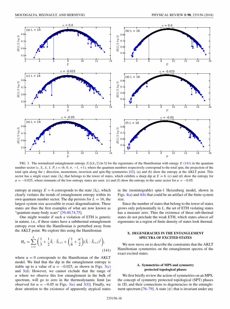
FIG. 3. The normalized entanglement entropy S/[(L/2) ln 3] for the eigenstates of the Hamiltonian with energy E (141) in the quantumnumber sector (s, Sz, k, I, Pz ) = (6, 0, π, −1, +1), where the quantum numbers respectively correspond to the total spin, the projection of thetotal spin along the z direction, momentum, inversion and spin-flip symmetries [42]. (a) and (b) show the entropy at the AKLT point. Thissector has a single exact state |S6〉 that belongs to the tower of states, which exhibits a sharp dip at E = 6. (c) and (d) show the entropy forα = −0.025, where remnants of the low-entropy states are seen. (e) and (f) show the entropy in the same sector for α = −0.05.
entropy at energy E = 6 corresponds to the state |S6〉, whichclearly violates the trends of entanglement entropy within itsown quantum number sector. The dip persists for L = 16, thelargest system size accessible to exact diagonalization. Thesestates are thus the first examples of what are now known as“quantum many-body scars” [39,40,74,75].
One might wonder if such a violation of ETH is genericin nature, i.e., if these states have a subthermal entanglemententropy even when the Hamiltonian is perturbed away fromthe AKLT point. We explore this using the Hamiltonian
Hα =L∑
i=1
(1
3+ 1
2�Si · �Si+1 +
(1
6+ α
2
)(�Si · �Si+1)2
),
(141)
where α = 0 corresponds to the Hamiltonian of the AKLTmodel. We find that the dip in the entanglement entropy isstable up to a value of α = −0.025, as shown in Figs. 3(c)and 3(d). However, we cannot exclude that the range ofα where we observe this low entanglement in the bulk ofspectrum, will go to zero in the thermodynamic limit [asobserved for α = −0.05 in Figs. 3(e) and 3(f)]. Finally, wedraw attention to the existence of apparently atypical states
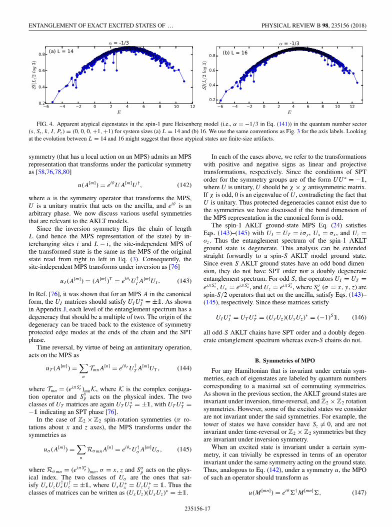
in the (nonintegrable) spin-1 Heisenberg model, shown inFigs. 4(a) and 4(b) that could be an artifact of the finite systemsize.
Since the number of states that belong to the tower of statesgrows only polynomially in L, the set of ETH violating stateshas a measure zero. Thus the existence of these sub-thermalstates do not preclude the weak ETH, which states almost alleigenstates in a region of finite density of states look thermal.
X. DEGENERACIES IN THE ENTANGLEMENTSPECTRA OF EXCITED STATES
We now move on to describe the constraints that the AKLTHamiltonian symmetries on the entanglement spectra of theexact excited states.
A. Symmetries of MPS and symmetryprotected topological phases
We first briefly review the action of symmetries on an MPS,the concept of symmetry protected topological (SPT) phasesin 1D, and their connections to degeneracies in the entangle-ment spectrum [76–79]. A state |ψ〉 that is invariant under any
235156-16
ENTANGLEMENT OF EXACT EXCITED STATES OF … PHYSICAL REVIEW B 98, 235156 (2018)
FIG. 4. Apparent atypical eigenstates in the spin-1 pure Heisenberg model (i.e., α = −1/3 in Eq. (141)) in the quantum number sector(s, Sz, k, I, Pz ) = (0, 0, 0, +1, +1) for system sizes (a) L = 14 and (b) 16. We use the same conventions as Fig. 3 for the axis labels. Lookingat the evolution between L = 14 and 16 might suggest that those atypical states are finite-size artifacts.
symmetry (that has a local action on an MPS) admits an MPSrepresentation that transforms under the particular symmetryas [58,76,78,80]
u(A[m] ) = eiθUA[m]U †, (142)
where u is the symmetry operator that transforms the MPS,U is a unitary matrix that acts on the ancilla, and eiθ is anarbitrary phase. We now discuss various useful symmetriesthat are relevant to the AKLT models.
Since the inversion symmetry flips the chain of lengthL (and hence the MPS representation of the state) by in-terchanging sites i and L − i, the site-independent MPS ofthe transformed state is the same as the MPS of the originalstate read from right to left in Eq. (3). Consequently, thesite-independent MPS transforms under inversion as [76]
uI (A[m] ) = (A[m] )T = eiθI U†I A
[m]UI . (143)
In Ref. [76], it was shown that for an MPS A in the canonicalform, the UI matrices should satisfy UIU
∗I = ±1. As shown
in Appendix J, each level of the entanglement spectrum has adegeneracy that should be a multiple of two. The origin of thedegeneracy can be traced back to the existence of symmetryprotected edge modes at the ends of the chain and the SPTphase.
Time reversal, by virtue of being an antiunitary operation,acts on the MPS as
uT (A[m] ) =∑
n
TmnA[n] = eiθT U
†T A[m]UT , (144)
where Tmn = (eiπSyp )mnK, where K is the complex conjuga-
tion operator and Syp acts on the physical index. The two
classes of UT matrices are again UT U ∗T = ±1, with UT U ∗
T =−1 indicating an SPT phase [76].
In the case of Z2 × Z2 spin-rotation symmetries (π ro-tations about x and z axes), the MPS transforms under thesymmetries as
uσ (A[m] ) =∑
n
Rσ mnA[n] = eiθσ U †
σA[m]Uσ , (145)
where Rσ mn = (eiπSσp )mn, σ = x, z and Sσ
p acts on the phys-ical index. The two classes of Uσ are the ones that sat-isfy UxUzU
†xU
†z = ±1, where UxU
∗x = UzU
∗z = 1. Thus the
classes of matrices can be written as (UxUz)(UxUz)∗ = ±1.
In each of the cases above, we refer to the transformationswith positive and negative signs as linear and projectivetransformations, respectively. Since the conditions of SPTorder for the symmetry groups are of the form UU ∗ = −1,where U is unitary, U should be χ × χ antisymmetric matrix.If χ is odd, 0 is an eigenvalue of U , contradicting the fact thatU is unitary. Thus protected degeneracies cannot exist due tothe symmetries we have discussed if the bond dimension ofthe MPS representation in the canonical form is odd.
The spin-1 AKLT ground-state MPS Eq. (24) satisfiesEqs. (143)–(145) with UI = UT = iσy , Ux = σx , and Uz =σz. Thus the entanglement spectrum of the spin-1 AKLTground state is degenerate. This analysis can be extendedstraight forwardly to a spin-S AKLT model ground state.Since even S AKLT ground states have an odd bond dimen-sion, they do not have SPT order nor a doubly degenerateentanglement spectrum. For odd S, the operators UI = UT =eiπS
ya , Ux = eiπSx
a , and Uz = eiπSza , where Sσ
a (σ = x, y, z) arespin-S/2 operators that act on the ancilla, satisfy Eqs. (143)–(145), respectively. Since these matrices satisfy
UIU∗I = UT U ∗
T = (UxUz)(UxUz)∗ = (−1)S1, (146)
all odd-S AKLT chains have SPT order and a doubly degen-erate entanglement spectrum whereas even-S chains do not.
B. Symmetries of MPO
For any Hamiltonian that is invariant under certain sym-metries, each of eigenstates are labeled by quantum numberscorresponding to a maximal set of commuting symmetries.As shown in the previous section, the AKLT ground states areinvariant under inversion, time-reversal, and Z2 × Z2 rotationsymmetries. However, some of the excited states we considerare not invariant under the said symmetries. For example, thetower of states we have consider have Sz �= 0, and are notinvariant under time-reversal or Z2 × Z2 symmetries but theyare invariant under inversion symmetry.
When an excited state is invariant under a certain sym-metry, it can trivially be expressed in terms of an operatorinvariant under the same symmetry acting on the ground state.Thus, analogous to Eq. (142), under a symmetry u, the MPOof such an operator should transform as
u(M [mn] ) = ei�M [mn]�, (147)
235156-17
MOUDGALYA, REGNAULT, AND BERNEVIG PHYSICAL REVIEW B 98, 235156 (2018)
where u acts on the physical indices of the MPO and � on theancilla.
We first discuss the symmetries that we discussed withregard to MPS in Sec. X A, i.e., inversion, time reversal, andZ2 × Z2 rotation. The actions of these symmetries on an MPOare similar to the actions on the MPS. Inversion symmetryinterchanges the operators acting on sites i and L − i. Thus,similar to Eq. (143), we obtain
uI (M [mn] ) = (M [mn] )T = eiθI �†IM
[mn]�I . (148)
Time-reversal and Z2 × Z2 rotation symmetries act on thephysical indices of the MPO via conjugation as
uT (M [mn] ) =∑l,k
TmlM[lk]T †
kn = eiθT �†T M [mn]�T (149)
and
uσ (M [mn] ) =∑l,k
Rσ mlM[lk]R†
σ kn = eiθσ �†σM [mn]�σ ,
(150)
where Tmn = (eiπSyp )m,nK, Rσ mn = (eiπSσ
p )mn, σ = x, z acton the physical index of the MPO. In each of these cases,the auxiliary indices of the MPO transform under the �I ,�T , �x , �z matrices under the various symmetries respec-tively. Similar to the case of an MPS, we could have MPOsthat transform in two distinct ways �I�
∗I = ±1, �T �∗
T =±1, and (�x�z)(�x�z)∗ = ±1. We refer to the transfor-mation with the positive and negative signs as linear andprojective MPO transformations, respectively. Thus, underphysical symmetries, if an MPS transforms on the ancillaunder U , and an MPO transforms under �, the MPO ×MPS transforms on the ancilla under U ⊗ �. As a con-sequence, if an MPO transforms projectively (respectively,linearly), the MPO × MPS transforms in a different (respec-tively, the same) way as the MPS.
For example, the MPO corresponding to the Arovas Aoperator [see Eq. (48)] transforms linearly under inversion,time-reversal and Z2 × Z2 rotation symmetries, and the trans-formation matrices are shown in Eqs. (I3), (I11), and (I16),respectively. The Arovas B operator [see Eq. (53)] transformsprojectively under inversion, linearly under time-reversal androtation symmetries, and the transformation matrices areshown in Eqs. (I5), (I13), and (I17) respectively. The towerof states operator transforms projectively and linearly underinversion symmetry for odd and even N , respectively, with thetransformation matrices shown in Eq. (I7). The transformationmatrices are shown in Appendix I. Note that we do not claimany topological protection of these states. Indeed, they have adegenerate largest eigenvalue of the transfer matrix, leadingto long-range correlations that do not decay exponentially.We discuss the implications of these transformations to theexcited state entanglement spectrum in the next section usingconcrete examples from the AKLT models.
XI. FINITE-SIZE EFFECTS IN THE ENTANGLEMENTSPECTRA OF EXCITED STATES
We proceed to describe the finite-size effects andsymmetry-protected degeneracies in the entanglement spectra
of the exact excited states of the AKLT models. Since theexact entanglement spectra depend on the configuration of thefree boundary spins, we freeze them to their highest weightstates. Such a boundary configuration is inversion symmetric,although it violates time-reversal and Z2 × Z2 rotation sym-metries (on the edges only).
A. Spin-S AKLT ground states
As described in Sec. X A, the entanglement spectrum ofthe spin-S AKLT ground state consists of (S + 1) degeneratelevels in the thermodynamic limit. Generically, such a degen-eracy between (S + 1) levels is broken for a finite system.However, as shown in the thermodynamic limit in Ref. [76]and for a finite system in Appendix J, the entanglementspectrum is always doubly degenerate when symmetries actprojectively. Thus, for odd S, since inversion, time reversaland Z2 × Z2 act projectively [see Eq. (146)], the entangle-ment spectrum consists of (S + 1)/2 exactly degenerate dou-blets. For even-S, the entanglement spectrum need not consistof degenerate levels for generic configurations of boundaryspins, though some levels can be degenerate for particularchoices of the boundary spins. While the exact form of thesplitting between the entanglement spectrum levels dependson the configuration of the boundary spins, we find that it isexponentially small in the system size.
B. Spin-1 AKLT tower of states
We first describe the entanglement spectrum of the spin-2magnon state of spin-1 AKLT model, |S2〉. In Sec. VI, we haveseen that the entanglement spectrum of such a state consistsof two copies of the ground-state entanglement spectrum. Fora finite n, using an explicit computation of ρred using themethods described in Sec. V B and illustrated in Appendix C,with MPS boundary vectors of Eq. (26), the four normalizedeigenvalues of ρred read [see Eq. (C14)]
2 ×(
n
4n − 3,
3 − 2n
6 − 8n
), (151)
where 2× indicates two copies. In Eq. (151), we have ignoredexponentially small finite-size splitting to obtain a closed formexpression. The two degenerate copies of the entanglementspectrum thus split into two doublets that have an O(1/n)(power-law) splitting. Similarly, the six eigenvalues of ρred for|S4〉 read
2 ×(
4n2 − 22n + 27
32n2 − 88n + 54,
2n2 − 5n
16n2 − 44n + 27,
4n2 − 6n
16n2 − 44n + 27
). (152)
This is consistent with the n → ∞ behavior calculated inSec. VIII B, i.e., the entanglement spectrum is composed ofthree copies of the ground state split into three doublets,two of which are degenerate in the thermodynamic limit athalf the entanglement energy of the other. The doublets thatare degenerate in the thermodynamic limit have an O(1/n)finite-size splitting between them.
More generically, we observe the following pattern in theentanglement spectrum of |S2N 〉. The (N + 1) copies of the
235156-18
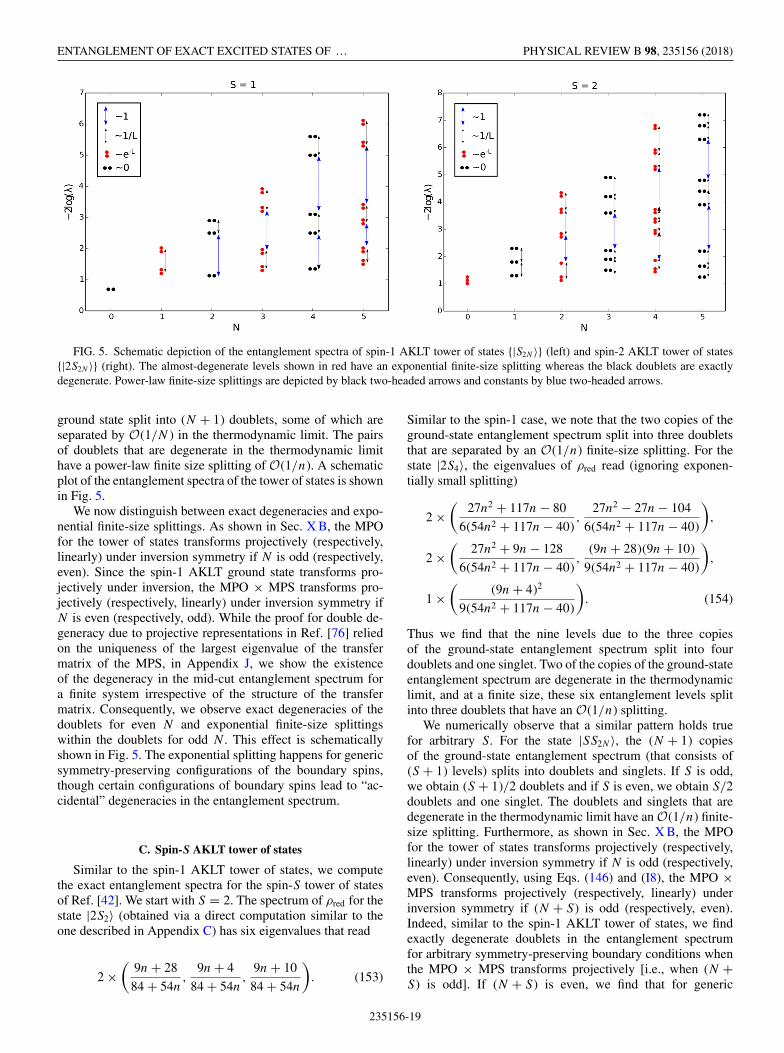
ENTANGLEMENT OF EXACT EXCITED STATES OF … PHYSICAL REVIEW B 98, 235156 (2018)
FIG. 5. Schematic depiction of the entanglement spectra of spin-1 AKLT tower of states {|S2N 〉} (left) and spin-2 AKLT tower of states{|2S2N 〉} (right). The almost-degenerate levels shown in red have an exponential finite-size splitting whereas the black doublets are exactlydegenerate. Power-law finite-size splittings are depicted by black two-headed arrows and constants by blue two-headed arrows.
ground state split into (N + 1) doublets, some of which areseparated by O(1/N ) in the thermodynamic limit. The pairsof doublets that are degenerate in the thermodynamic limithave a power-law finite size splitting of O(1/n). A schematicplot of the entanglement spectra of the tower of states is shownin Fig. 5.
We now distinguish between exact degeneracies and expo-nential finite-size splittings. As shown in Sec. X B, the MPOfor the tower of states transforms projectively (respectively,linearly) under inversion symmetry if N is odd (respectively,even). Since the spin-1 AKLT ground state transforms pro-jectively under inversion, the MPO × MPS transforms pro-jectively (respectively, linearly) under inversion symmetry ifN is even (respectively, odd). While the proof for double de-generacy due to projective representations in Ref. [76] reliedon the uniqueness of the largest eigenvalue of the transfermatrix of the MPS, in Appendix J, we show the existenceof the degeneracy in the mid-cut entanglement spectrum fora finite system irrespective of the structure of the transfermatrix. Consequently, we observe exact degeneracies of thedoublets for even N and exponential finite-size splittingswithin the doublets for odd N . This effect is schematicallyshown in Fig. 5. The exponential splitting happens for genericsymmetry-preserving configurations of the boundary spins,though certain configurations of boundary spins lead to “ac-cidental” degeneracies in the entanglement spectrum.
C. Spin-S AKLT tower of states
Similar to the spin-1 AKLT tower of states, we computethe exact entanglement spectra for the spin-S tower of statesof Ref. [42]. We start with S = 2. The spectrum of ρred for thestate |2S2〉 (obtained via a direct computation similar to theone described in Appendix C) has six eigenvalues that read
2 ×(
9n + 28
84 + 54n,
9n + 4
84 + 54n,
9n + 10
84 + 54n
). (153)
Similar to the spin-1 case, we note that the two copies of theground-state entanglement spectrum split into three doubletsthat are separated by an O(1/n) finite-size splitting. For thestate |2S4〉, the eigenvalues of ρred read (ignoring exponen-tially small splitting)
2 ×(
27n2 + 117n − 80
6(54n2 + 117n − 40),
27n2 − 27n − 104
6(54n2 + 117n − 40)
),
2 ×(
27n2 + 9n − 128
6(54n2 + 117n − 40),
(9n + 28)(9n + 10)
9(54n2 + 117n − 40)
),
1 ×(
(9n + 4)2
9(54n2 + 117n − 40)
). (154)
Thus we find that the nine levels due to the three copiesof the ground-state entanglement spectrum split into fourdoublets and one singlet. Two of the copies of the ground-stateentanglement spectrum are degenerate in the thermodynamiclimit, and at a finite size, these six entanglement levels splitinto three doublets that have an O(1/n) splitting.
We numerically observe that a similar pattern holds truefor arbitrary S. For the state |SS2N 〉, the (N + 1) copiesof the ground-state entanglement spectrum (that consists of(S + 1) levels) splits into doublets and singlets. If S is odd,we obtain (S + 1)/2 doublets and if S is even, we obtain S/2doublets and one singlet. The doublets and singlets that aredegenerate in the thermodynamic limit have an O(1/n) finite-size splitting. Furthermore, as shown in Sec. X B, the MPOfor the tower of states transforms projectively (respectively,linearly) under inversion symmetry if N is odd (respectively,even). Consequently, using Eqs. (146) and (I8), the MPO ×MPS transforms projectively (respectively, linearly) underinversion symmetry if (N + S) is odd (respectively, even).Indeed, similar to the spin-1 AKLT tower of states, we findexactly degenerate doublets in the entanglement spectrumfor arbitrary symmetry-preserving boundary conditions whenthe MPO × MPS transforms projectively [i.e., when (N +S) is odd]. If (N + S) is even, we find that for generic
235156-19

MOUDGALYA, REGNAULT, AND BERNEVIG PHYSICAL REVIEW B 98, 235156 (2018)
symmetry-preserving boundary conditions, we obtain an ex-ponential finite-size splitting between the doublets that aredegenerate in the thermodynamic limit.
D. Spin-1 Arovas states
For the spin-1 Arovas A state, via a direct computationsimilar to the example in Appendix C, we find that the eighteigenvalues of ρred read
2 ×(
n + 3 + 2√
2(1 + n)
4n + 14,n + 3 − 2
√2(1 + n)
4n + 14
),
4 ×(
1
8n + 28
). (155)
Thus, similar to the spin-2 magnon, we obtain two copiesof the ground-state entanglement spectrum that splits intotwo doublets that have an O(1/
√n) splitting between them.
In addition, we obtain four entanglement levels that are ofO(1/n). As mentioned in Sec. X B, the Arovas A MPOtransforms linearly under inversion, time-reversal, and Z2 ×Z2 symmetries. Consequently, the MPO × MPS transformsprojectively and all the doublets are exactly degenerate for afinite system.
While we were not able to obtain a closed-form expressionfor the entanglement spectra of the spin-1 and spin-2 Arovas Bstates [42], we numerically observe similar phenomenology asthe Arovas A and the spin-2S magnon entanglement spectra,although the magnitude of the finite-size splittings [O(1/
√n)
versus O(1/n)] are not clear.
XII. CONCLUSION
We have computed the entanglement spectra of the exactexcited states of the AKLT models that were derived inRef. [42]. To achieve this, we expressed the states as MPO ×MPS’ and developed a general formalism to compute theentanglement spectra of states using the Jordan normal formof the MPO × MPS transfer matrix. We first exemplifiedour method by reproducing existing results on single-modeexcitations: we show that their entanglement spectra in thethermodynamic limit consist of two copies of the ground-stateentanglement spectrum. The low-lying exact excited statesof the AKLT model such as the Arovas states and the spin-2S magnon states for the spin-S AKLT chain fall into thiscategory. For single-mode excitations, our method is exactlyequivalent to the tangent-space and related methods developedto numerically as well as analytically probe low-energy ex-cited states in the MPS formalism [22,24–27,67,81,82]. Wenote that our method can be applied to obtain results onthe entanglement spectra of single-mode excitations in thefractional quantum Hall effect [72,83].
We then generalized our method to states with multiplemagnons, that are beyond single-mode excitations (“doubletangent space” [84] and beyond). This allowed us to obtainthe exact expression for the entanglement spectra for thespin-S AKLT tower of states for a zero density of magnons inthe thermodynamic limit. We showed that the entanglementspectrum of the N th state of the tower consists of (N + 1)copies of the ground-state entanglement spectrum, not alldegenerate. Apart from the specific Jordan block structure
derived for the special AKLT tower of states, our methodto obtain the entanglement spectrum was completely general.In particular, it applies to states of the form ON |ψ〉, whereO is any translation invariant operator and |ψ〉 is a statethat admits a site-independent MPS representation. Moreover,since the entanglement entropy of the AKLT tower of statesin Eq. (135) has a similar form as the entanglement entropyin equal-momentum quasiparticle excited states of free-fieldtheories and certain integrable models [85–88], it is likelythat our formulas for the entanglement spectrum and entropyholds in more general integrable and nonintegrable modelsfor equal-momentum quasiparticle excited states in the zerodensity limit. We defer the exploration of equal and unequalmomentum quasiparticle excited states using our formalism ina generic setting to future work. For the AKLT tower of states,we also showed that the replica structure of the entanglementspectra of the tower of states persists in the thermodynamiclimit only for states at a zero energy density, conforming withfolklore that only low-energy excitations resemble the groundstate. An interesting problem is to prove this on generalgrounds for excited states in integrable and/or nonintegrablemodels. Moreover, since the exact excited states of the AKLTmodel have noninjective matrix-product expressions with fi-nite bond dimensions, perhaps one could obtain a class ofnoninjective matrix-product states that describe excited states,similar to a classification of matrix-product ground states[89,90].
We also studied finite-size effects in the entanglementspectra of these states and showed a universal power-lawsplitting between the different copies of the ground state. Weidentified exact degeneracies and exponential splittings basedon projective versus linear transformations of the MPO ×MPS at a finite size. While protected exact degeneracies inthe entanglement spectrum of excited states are reminiscentof SPT phases for the ground states, it is unclear if these havea topological origin in the excited states, given that excitedstates do not have a protecting gap.
We emphasized that the states of the tower have an entan-glement entropy that scales as S ∝ log L, which is incom-patible with strong ETH, if these states indeed exist in thebulk of the energy spectrum [42]. Further, we showed thatthe violation of ETH seems to persist for SU(2) symmetricspin-1 Hamiltonians slightly away from the AKLT point, andwe pointed out numerically apparent low-entropy states in thepure Heisenberg model, far away from the AKLT point. How-ever, a systematic numerical study of these low-entropy statesaway from the AKLT point is necessitated, with and withoutbreaking the SU(2) symmetry. These special states, first ob-tained in Ref. [42], provide analytically tractable examplesof “quantum many-body scars,” described in Refs. [39,74].While such anomalous eigenstates are known to exist insingle-particle chaotic systems, very few examples are knownin many-body quantum systems [91]. An interesting problemis to determine if these anomalous states play any interestingrole in the dynamics of the AKLT models [39,40,75].
ACKNOWLEDGMENTS
We thank Yang-Le Wu for an initial collaboration, StephanRachel for collaboration on related work and David Huse,
235156-20

ENTANGLEMENT OF EXACT EXCITED STATES OF … PHYSICAL REVIEW B 98, 235156 (2018)
FIG. 6. Labelling in the MPS construction of the spin-S AKLTground state. Big and small circles represent physical spin-S andvirtual spin-S/2 degrees of freedom, respectively.
Shivaji Sondhi and Michael Zaletel for useful discussions.BAB wishes to thank Ecole Normale Superieure, UPMCParis, and Donostia International Physics Center for theirgenerous sabbatical hosting during some of the stages ofthis work. BAB acknowledges support for the analytic workDepartment of Energy de-sc0016239, Simons InvestigatorAward, the Packard Foundation, and the Schmidt Fund forInnovative Research. The computational part of the Prince-ton work was performed under NSF EAGER Grant No.DMR-1643312, No. ONR-N00014-14-1-0330, and No. NSF-MRSEC DMR-1420541.
APPENDIX A: MATRIX PRODUCT STATES FOR SPIN-SAKLT GROUND STATES
In this section, we derive the matrix product state (MPS)representations and the structure of the transfer matrix for thespin-S AKLT ground states with open boundary conditions(OBC). We follow the derivation in Ref. [30]. Similar expres-sions can be obtained by alternate methods in the literature[60,92–96].
1. MPS
As mentioned in Sec. III, each spin-S can be viewed as twosymmetrized spin-S/2 bosons. The AKLT ground state is thena product of spin-S/2 singlets, i.e., the J = 0 state formed bytwo spin-S/2 on nearest neighbor spin-S (see Fig. 2). We usethe labels ui and vi to denote the Sz values of the left and rightspin-S/2 on site i, respectively (see Fig. 6). Thus the spin-S/2
singlet state |0 0〉S2i,i+1 formed between the spin-S/2’s vi and
ui+1 can be written in the Sz basis of spin-S/2 (denoted by|vi, ui+1〉 S
2) as
|0 0〉S/2i,i+1 =
S2∑
α=− S2
S2〈α,−α|0 0〉|α,−α〉i,i+1
≡∑
vi ,ui+1
�S2vi ,ui+1 |vi, ui+1〉 S
2, (A1)
where s〈s1, s2|J Jz〉 is the Clebsch-Gordan coefficient for twospin-s with Sz = s1 and Sz = s2 to form a state with total spinJ and Sz = Jz = s1 + s2. The matrix � thus assumes the form
�S2αβ = S
2〈α, β|0 0〉δα,−β, (A2)
where the indices −S/2 � α, β � S/2. For example, for S =1 (the spin-1 AKLT ground state), we know that vi, ui+1 =↑,↓ and the singlet |0 0〉
12i,i+1 can be written as
|0 0〉12i,i+1 = |vi = ↑, ui+1 = ↓〉 − |vi = ↓, ui+1 = ↑〉√
2.
(A3)
For S = 1, the matrix �12 thus reads
�12 =
(0 1√
2− 1√
20
). (A4)
In terms of these matrices, the spin-S AKLT ground state|SG〉 S
2in the spin- S
2 basis with OBC and the edge spins bothhaving Sz = S/2 (denoted by |S/2〉1 and |S/2〉L) reads
|SG〉 S2
= |S/2〉1
L−1∏i=1
|0 0〉S2i,i+1|S/2〉L
=∑
{ui ,vi }δu1,
S2�
S2v1u2 . . . �
S2vL−1uL
δvL, S2|{ui, vi}〉 S
2, (A5)
where |{ui, vi}〉 S2
= |u1, v1, . . . , uL, vL〉 S2. The ground state
can be written in the onsite spin-S basis using a projector
P(S, S
2 )i to symmetrize the two spin-S/2 on each site, where
the projector reads
P(S, S
2 )i =
∑mi
∑uivi
M [mi ]ui ,vi
|mi〉S S2〈ui, vi |, (A6)
where |mi〉S denotes the spin-S state on site i with Sz = mi .The tensor M assumes the form
M[m]αβ = 〈S m|α, β〉 S
2δm,α+β. (A7)
For example, for S = 1, the projector P(1, 1
2 )i reads
P(1, 1
2 )i = |mi = 1〉1 1
2〈ui = ↑, vi = ↑|
+ |mi = 0〉1
12〈ui = ↑, vi = ↓| + 1
2〈ui = ↓, vi = ↑|
√2
+ |mi = −1〉1 12〈ui = ↓, vi = ↓|. (A8)
The matrices M for S = 1 thus read
M [1] =(
1 00 0
),
M [0] =(
0 1√2
1√2
0
), (A9)
M [−1] =(
0 00 1
).
The projector on the full state, P (S, S2 ) = ∏
i P(S, S
2 )i is then
P (S, S2 ) =
∑{mi }
∑{uivi }
M [m1]u1v1
. . . M [mL]uLvL
|{mi}〉S S2〈{ui, vi}|,
(A10)
where |{mi}〉S = |m1,m2, . . . , mL〉S . The ground state in thespin-S basis |SG〉S = P|SG〉 S
2reads
|SG〉S =∑{mi }
∑{ui ,vi }
(δu1,S/2M
[m1]u1v1
�S2v1u2M
[m2]u2v2
. . .
�S2vL−1uL
M [mL]uLvL
δvL,S/2)|{mi}〉S
=∑
{mi,ui }bl
Au1A[m1]
u1u2. . . A[mL]
uL−1uLbr
uL|{mi}〉S, (A11)
235156-21
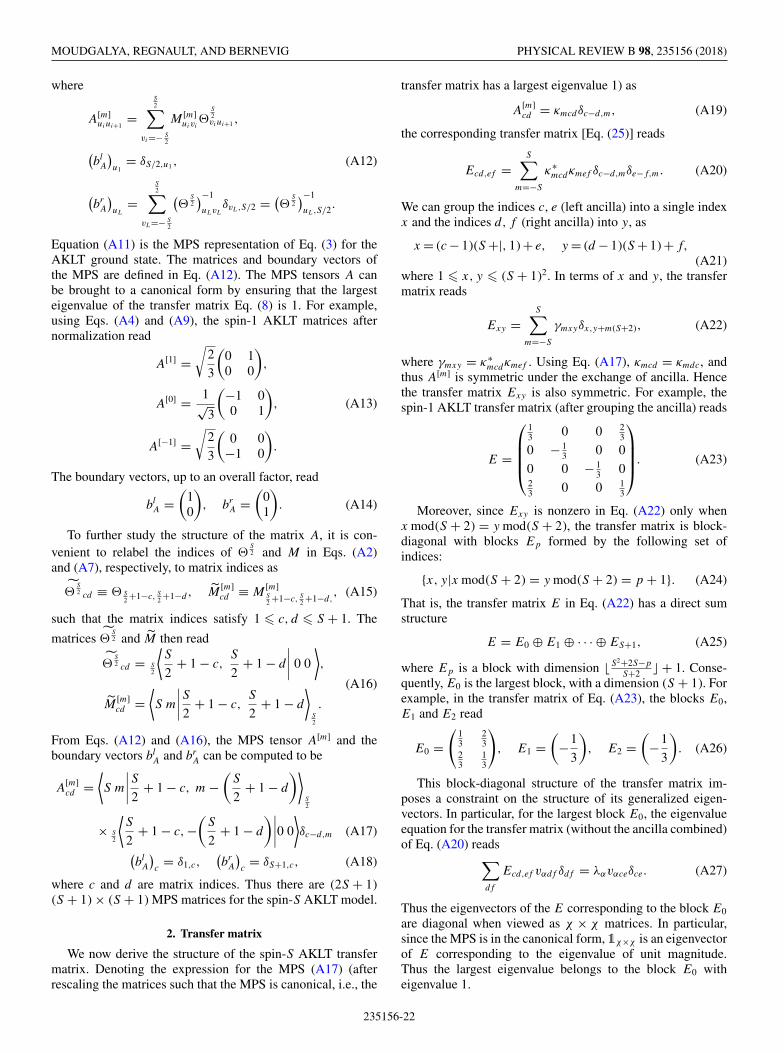
MOUDGALYA, REGNAULT, AND BERNEVIG PHYSICAL REVIEW B 98, 235156 (2018)
where
A[m]uiui+1
=S2∑
vi=− S2
M [m]uivi
�S2viui+1 ,
(bl
A
)u1
= δS/2,u1 , (A12)
(br
A
)uL
=S2∑
vL=− S2
(�
S2)−1
uLvLδvL,S/2 = (
�S2)−1
uL,S/2.
Equation (A11) is the MPS representation of Eq. (3) for theAKLT ground state. The matrices and boundary vectors ofthe MPS are defined in Eq. (A12). The MPS tensors A canbe brought to a canonical form by ensuring that the largesteigenvalue of the transfer matrix Eq. (8) is 1. For example,using Eqs. (A4) and (A9), the spin-1 AKLT matrices afternormalization read
A[1] =√
2
3
(0 10 0
),
A[0] = 1√3
(−1 00 1
), (A13)
A[−1] =√
2
3
(0 0
−1 0
).
The boundary vectors, up to an overall factor, read
blA =
(10
), br
A =(
01
). (A14)
To further study the structure of the matrix A, it is con-venient to relabel the indices of �
S2 and M in Eqs. (A2)
and (A7), respectively, to matrix indices as
�S2 cd ≡ � S
2 +1−c, S2 +1−d , M
[m]cd ≡ M
[m]S2 +1−c, S
2 +1−d,, (A15)
such that the matrix indices satisfy 1 � c, d � S + 1. The
matrices �S2 and M then read
�S2 cd = S
2
⟨S
2+ 1 − c,
S
2+ 1 − d
∣∣∣∣ 0 0
⟩,
(A16)
M[m]cd =
⟨S m
∣∣∣∣S2 + 1 − c,S
2+ 1 − d
⟩S2
.
From Eqs. (A12) and (A16), the MPS tensor A[m] and theboundary vectors bl
A and brA can be computed to be
A[m]cd =
⟨S m
∣∣∣∣S2 + 1 − c, m −(
S
2+ 1 − d
)⟩S2
× S2
⟨S
2+ 1 − c,−
(S
2+ 1 − d
)∣∣∣∣0 0
⟩δc−d,m (A17)(
blA
)c
= δ1,c,(br
A
)c= δS+1,c, (A18)
where c and d are matrix indices. Thus there are (2S + 1)(S + 1) × (S + 1) MPS matrices for the spin-S AKLT model.
2. Transfer matrix
We now derive the structure of the spin-S AKLT transfermatrix. Denoting the expression for the MPS (A17) (afterrescaling the matrices such that the MPS is canonical, i.e., the
transfer matrix has a largest eigenvalue 1) as
A[m]cd = κmcdδc−d,m, (A19)
the corresponding transfer matrix [Eq. (25)] reads
Ecd,ef =S∑
m=−S
κ∗mcdκmef δc−d,mδe−f,m. (A20)
We can group the indices c, e (left ancilla) into a single indexx and the indices d, f (right ancilla) into y, as
x = (c − 1)(S +|, 1) + e, y = (d − 1)(S + 1) + f,
(A21)where 1 � x, y � (S + 1)2. In terms of x and y, the transfermatrix reads
Exy =S∑
m=−S
γmxyδx,y+m(S+2), (A22)
where γmxy = κ∗mcdκmef . Using Eq. (A17), κmcd = κmdc, and
thus A[m] is symmetric under the exchange of ancilla. Hencethe transfer matrix Exy is also symmetric. For example, thespin-1 AKLT transfer matrix (after grouping the ancilla) reads
E =
⎛⎜⎜⎜⎝13 0 0 2
3
0 − 13 0 0
0 0 − 13 0
23 0 0 1
3
⎞⎟⎟⎟⎠. (A23)
Moreover, since Exy is nonzero in Eq. (A22) only whenx mod(S + 2) = y mod(S + 2), the transfer matrix is block-diagonal with blocks Ep formed by the following set ofindices:
{x, y|x mod(S + 2) = y mod(S + 2) = p + 1}. (A24)
That is, the transfer matrix E in Eq. (A22) has a direct sumstructure
E = E0 ⊕ E1 ⊕ · · · ⊕ ES+1, (A25)
where Ep is a block with dimension � S2+2S−p
S+2 � + 1. Conse-quently, E0 is the largest block, with a dimension (S + 1). Forexample, in the transfer matrix of Eq. (A23), the blocks E0,E1 and E2 read
E0 =(
13
23
23
13
), E1 =
(−1
3
), E2 =
(−1
3
). (A26)
This block-diagonal structure of the transfer matrix im-poses a constraint on the structure of its generalized eigen-vectors. In particular, for the largest block E0, the eigenvalueequation for the transfer matrix (without the ancilla combined)of Eq. (A20) reads∑
df
Ecd,ef vαdf δdf = λαvαceδce. (A27)
Thus the eigenvectors of the E corresponding to the block E0
are diagonal when viewed as χ × χ matrices. In particular,since the MPS is in the canonical form, 1χ×χ is an eigenvectorof E corresponding to the eigenvalue of unit magnitude.Thus the largest eigenvalue belongs to the block E0 witheigenvalue 1.
235156-22
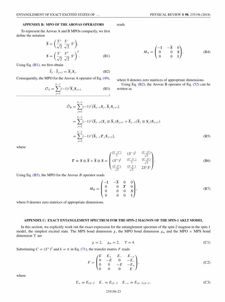
ENTANGLEMENT OF EXACT EXCITED STATES OF … PHYSICAL REVIEW B 98, 235156 (2018)
APPENDIX B: MPO OF THE AROVAS OPERATORS
To represent the Arovas A and B MPOs compactly, we firstdefine the notation
S =(
S+√
2
S−√
2Sz
),
S =(
S−√
2
S+√
2Sz
)T
. (B1)
Using Eq. (B1), we first obtain
�Sj · �Sj+1 = Sj Sj . (B2)
Consequently, the MPO for the Arovas A operator of Eq. (49),
OA =L−1∑j=1
(−1)j Sj Sj+1 (B3)
reads
MA =⎛⎝−1 −S 0
0 0 S0 0 1
⎞⎠, (B4)
where 0 denotes zero matrices of appropriate dimensions.Using Eq. (B2), the Arovas B operator of Eq. (52) can be
written as
OB =L−1∑j=2
(−1)j {Sj−1 Sj , Sj Sj+1}
=L−1∑j=2
(−1)j (Sj−1(Sj ⊗ Sj )Sj+1 + Sj−1(Sj ⊗ Sj )Sj+1)
=L−1∑j=2
(−1)j {Sj−1T j Sj+1}, (B5)
where
T ≡ S ⊗ S + S ⊗ S =
⎛⎜⎜⎝{S−,S+}
2 (S−)2 {S−,Sz}√2
(S+)2 {S+,S−}2
{S+,Sz}√2
{Sz,S+}√2
{Sz,S−}√2
2SzSz
⎞⎟⎟⎠. (B6)
Using Eq. (B5), the MPO for the Arovas B operator reads
MB =
⎛⎜⎜⎝−1 −S 0 00 0 T 00 0 0 S0 0 0 1
⎞⎟⎟⎠, (B7)
where 0 denotes zero matrices of appropriate dimensions.
APPENDIX C: EXACT ENTANGLEMENT SPECTRUM FOR THE SPIN-2 MAGNON OF THE SPIN-1 AKLT MODEL
In this section, we explicitly work out the exact expression for the entanglement spectrum of the spin-2 magnon in the spin-1model, the simplest excited state. The MPS bond dimension χ , the MPO bond dimension χm and the MPO × MPS bonddimension ϒ are
χ = 2, χm = 2, ϒ = 4. (C1)
Substituting C = (S+)2 and k = π in Eq. (71), the transfer matrix F reads
F =
⎛⎜⎝E E+ E− E−+0 −E 0 −E−0 0 −E −E+0 0 0 E
⎞⎟⎠, (C2)
where
E+ ≡ E(S+ )2 E− ≡ E(S− )2 E−+ ≡ E(S− )2(S+ )2 , (C3)
235156-23

MOUDGALYA, REGNAULT, AND BERNEVIG PHYSICAL REVIEW B 98, 235156 (2018)
shown in Eq. (E3). We refer to the blocks of F as the MPS blocks.The Jordan decomposition of F reads
F = PJP −1, (C4)
where J (obtained using symbolic calculations) reads
J =
⎛⎜⎜⎜⎜⎜⎜⎜⎜⎜⎜⎜⎜⎜⎜⎜⎜⎜⎜⎜⎜⎜⎜⎜⎜⎜⎜⎜⎜⎝
1 0 0 0 0 0 0 0 0 0 0 0 1 0 0 00 − 1
3 0 0 0 0 0 0 0 0 0 0 0 1 0 00 0 − 1
3 0 0 0 0 0 0 0 0 0 0 0 1 00 0 0 − 1
3 0 0 0 0 0 0 0 0 0 0 0 1
0 0 0 0 −1 0 0 0 0 0 0 0 0 0 0 00 0 0 0 0 1
3 0 0 0 0 0 0 0 0 0 00 0 0 0 0 0 1
3 0 0 0 0 0 0 0 0 00 0 0 0 0 0 0 1
3 0 0 0 0 0 0 0 0
0 0 0 0 0 0 0 0 −1 0 0 0 0 0 0 00 0 0 0 0 0 0 0 0 1
3 0 0 0 0 0 00 0 0 0 0 0 0 0 0 0 1
3 0 0 0 0 00 0 0 0 0 0 0 0 0 0 0 1
3 0 0 0 0
0 0 0 0 0 0 0 0 0 0 0 0 1 0 0 00 0 0 0 0 0 0 0 0 0 0 0 0 − 1
3 0 00 0 0 0 0 0 0 0 0 0 0 0 0 0 − 1
3 00 0 0 0 0 0 0 0 0 0 0 0 0 0 0 − 1
3
⎞⎟⎟⎟⎟⎟⎟⎟⎟⎟⎟⎟⎟⎟⎟⎟⎟⎟⎟⎟⎟⎟⎟⎟⎟⎟⎟⎟⎟⎠
, (C5)
and P , P −1 read
P =
⎛⎜⎜⎜⎜⎜⎜⎜⎜⎜⎜⎜⎜⎜⎜⎜⎜⎜⎜⎜⎜⎜⎜⎜⎜⎜⎝
1 0 0 −1 0 0 0 0 0 0 0 0 − 32 0 0 − 3
20 1 0 0 0 0 −1 0 0 0 0 0 0 0 0 00 0 1 0 0 0 0 0 0 −1 0 0 0 0 0 01 0 0 1 0 0 0 0 0 0 0 0 0 0 0 00 0 0 0 1 0 0 −1 0 0 0 0 0 0 0 00 0 0 0 0 1 0 0 0 0 0 0 0 0 0 00 0 0 0 0 0 1 0 0 0 0 0 0 − 3
2 0 00 0 0 0 1 0 0 1 0 0 0 0 0 0 0 00 0 0 0 0 0 0 0 1 0 0 −1 0 0 0 00 0 0 0 0 0 0 0 0 1 0 0 0 0 − 3
2 00 0 0 0 0 0 0 0 0 0 1 0 0 0 0 00 0 0 0 0 0 0 0 1 0 0 1 0 0 0 00 0 0 0 0 0 0 0 0 0 0 0 3 0 0 30 0 0 0 0 0 0 0 0 0 0 0 0 3
2 0 00 0 0 0 0 0 0 0 0 0 0 0 0 0 3
2 00 0 0 0 0 0 0 0 0 0 0 0 3 0 0 −3
⎞⎟⎟⎟⎟⎟⎟⎟⎟⎟⎟⎟⎟⎟⎟⎟⎟⎟⎟⎟⎟⎟⎟⎟⎟⎟⎠
,
P −1 =
⎛⎜⎜⎜⎜⎜⎜⎜⎜⎜⎜⎜⎜⎜⎜⎜⎜⎜⎜⎜⎜⎜⎜⎜⎜⎜⎜⎜⎝
12 0 0 1
2 0 0 0 0 0 0 0 0 14 0 0 0
0 1 0 0 0 0 0 0 1 0 0 0 0 1 0 00 0 1 0 0 0 0 0 0 1 0 0 0 0 1 0
− 12 0 0 1
2 0 0 0 0 0 0 0 0 − 14 0 0 0
0 0 0 0 12 0 0 1
2 0 0 0 0 0 0 0 00 0 0 0 0 1 0 0 0 0 0 0 0 0 0 00 0 0 0 0 0 1 0 0 0 0 0 0 1 0 00 0 0 0 − 1
2 0 0 12 0 0 0 0 0 0 0 0
0 0 0 0 0 0 0 0 12 0 0 1
2 0 0 0 00 0 0 0 0 0 0 0 0 1 0 0 0 0 1 00 0 0 0 0 0 0 0 0 0 1 0 0 0 0 00 0 0 0 0 0 0 0 − 1
2 0 0 12 0 0 0 0
0 0 0 0 0 0 0 0 0 0 0 0 16 0 0 1
60 0 0 0 0 0 0 0 0 0 0 0 0 2
3 0 00 0 0 0 0 0 0 0 0 0 0 0 0 0 2
3 00 0 0 0 0 0 0 0 0 0 0 0 1
6 0 0 − 16
⎞⎟⎟⎟⎟⎟⎟⎟⎟⎟⎟⎟⎟⎟⎟⎟⎟⎟⎟⎟⎟⎟⎟⎟⎟⎟⎟⎟⎠
, (C6)
235156-24

ENTANGLEMENT OF EXACT EXCITED STATES OF … PHYSICAL REVIEW B 98, 235156 (2018)
where in J , P , and P −1 the lines demarcate the MPS blocks. Using Eq. (C5), the truncated Jordan block Junit [defined in Eq. (78)]reads
Junit =
⎛⎜⎝1 0 0 10 −1 0 00 0 −1 00 0 0 1
⎞⎟⎠. (C7)
Using P and P −1 in Eq. (C6), VL and VR define in Eq. (83) read
VR =
⎛⎜⎜⎜⎜⎜⎜⎜⎜⎜⎜⎜⎜⎜⎜⎜⎜⎜⎜⎜⎜⎜⎜⎜⎜⎝
1 0 0 − 32
0 0 0 00 0 0 01 0 0 00 1 0 00 0 0 00 0 0 00 1 0 00 0 1 00 0 0 00 0 0 00 0 1 00 0 0 30 0 0 00 0 0 00 0 0 3
⎞⎟⎟⎟⎟⎟⎟⎟⎟⎟⎟⎟⎟⎟⎟⎟⎟⎟⎟⎟⎟⎟⎟⎟⎟⎠
, VL =
⎛⎜⎜⎜⎜⎜⎜⎜⎜⎜⎜⎜⎜⎜⎜⎜⎜⎜⎜⎜⎜⎜⎜⎜⎜⎜⎜⎝
12 0 0 00 0 0 00 0 0 012 0 0 0
0 12 0 0
0 0 0 00 0 0 00 1
2 0 0
0 0 12 0
0 0 0 00 0 0 00 0 1
2 014 0 0 1
60 0 0 00 0 0 00 0 0 1
6
⎞⎟⎟⎟⎟⎟⎟⎟⎟⎟⎟⎟⎟⎟⎟⎟⎟⎟⎟⎟⎟⎟⎟⎟⎟⎟⎟⎠
. (C8)
For simplicity, we assume that the boundary spin-1/2 arein the Sz = +1/2 configuration. Consequently, the boundaryvectors read [see Eq. (26)]
blA =
(10
), br
A =(
01
). (C9)
Consequently, using Eqs. (68) and (43), we obtain the 16-dimensional boundary vectors of the transfer matrix whosecomponents read
(bl
F
)i= δi,1,
(br
F
)i= δi,16. (C10)
Using
J nunit =
⎛⎜⎝1 0 0 n
0 (−1)n 0 00 0 (−1)n 00 0 0 1
⎞⎟⎠, (C11)
VR and VL from Eq. (C8) and the boundary vectors fromEq. (C10), Runit and Lunit in Eq. (85) (when viewed as ϒ2-
dimensional vectors) read
Runit =
⎛⎜⎜⎜⎜⎜⎜⎜⎜⎜⎜⎜⎜⎜⎜⎜⎜⎜⎜⎜⎜⎜⎜⎜⎜⎜⎝
n6 − 1
400n6
00000000120012
⎞⎟⎟⎟⎟⎟⎟⎟⎟⎟⎟⎟⎟⎟⎟⎟⎟⎟⎟⎟⎟⎟⎟⎟⎟⎟⎠
, Lunit =
⎛⎜⎜⎜⎜⎜⎜⎜⎜⎜⎜⎜⎜⎜⎜⎜⎜⎜⎜⎜⎜⎜⎜⎜⎜⎜⎝
120012
00000000n600
− 14 + n
6
⎞⎟⎟⎟⎟⎟⎟⎟⎟⎟⎟⎟⎟⎟⎟⎟⎟⎟⎟⎟⎟⎟⎟⎟⎟⎟⎠
, (C12)
where the lines demarcate the MPS blocks. Runit and Lunit
can be viewed as ϒ × ϒ matrices, where the MPS blocksare reshaped separately. That is, the reshaped ϒ × ϒ matricesRunit and Lunit read
Runit =
⎛⎜⎜⎝n6 − 1
4 0 0 00 n
6 0 0
0 0 12 0
0 0 0 12
⎞⎟⎟⎠,
Lunit =
⎛⎜⎜⎝12 0 0 00 1
2 0 00 0 n
6 00 0 0 n
6 − 14
⎞⎟⎟⎠. (C13)
235156-25
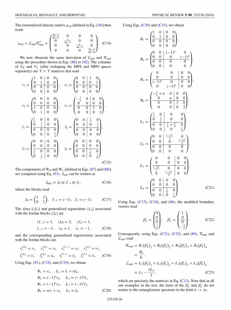
MOUDGALYA, REGNAULT, AND BERNEVIG PHYSICAL REVIEW B 98, 235156 (2018)
The (normalized) density matrix ρred [defined in Eq. (18)] thenreads
ρred = LunitRTunit =
⎛⎜⎜⎝2n−38n−6 0 0 0
0 n4n−3 0 0
0 0 n4n−3 0
0 0 0 2n−38n−6
⎞⎟⎟⎠. (C14)
We now illustrate the same derivation of Lunit and Runit
using the procedure shown in Eqs. (86) to (92). The columnsof VR and VL (after reshaping the MPS and MPO spacesseparately) are ϒ × ϒ matrices that read
r1 =
⎛⎜⎝1 0 0 00 1 0 00 0 0 00 0 0 0
⎞⎟⎠, r2 =
⎛⎜⎝0 0 1 00 0 0 10 0 0 00 0 0 0
⎞⎟⎠,
r3 =
⎛⎜⎝0 0 0 00 0 0 01 0 0 00 1 0 0
⎞⎟⎠, r4 =
⎛⎜⎜⎝− 3
2 0 0 00 0 0 00 0 3 00 0 0 3
⎞⎟⎟⎠,
l1 =
⎛⎜⎜⎝12 0 0 00 1
2 0 00 0 0 00 0 0 1
4
⎞⎟⎟⎠, l2 =
⎛⎜⎜⎝0 0 1
2 00 0 0 1
2
0 0 0 00 0 0 0
⎞⎟⎟⎠,
l3 =
⎛⎜⎜⎝0 0 0 00 0 0 012 0 0 00 1
2 0 0
⎞⎟⎟⎠, l4 =
⎛⎜⎜⎝0 0 0 00 0 0 0
0 0 16 0
0 0 0 16
⎞⎟⎟⎠.
(C15)
The components of WR and WL [defined in Eqs. (87) and (88)]are computed using Eq. (91). Junit can be written as
Junit = J0 ⊕ J−1 ⊕ J1, (C16)
where the blocks read
J0 =(
1 10 1
), J−1 = (−1), J1 = (−1). (C17)
The sizes {|Jk|} and generalized eigenvalues {λk} associatedwith the Jordan blocks {Jk} are
|J−1| = 1, |J0| = 2, |J1| = 1,
λ−1 = −1, λ0 = 1, λ1 = −1, (C18)
and the corresponding generalized eigenvectors associatedwith the Jordan blocks are
r(J0 )1 = r1, r
(J0 )2 = r4, r
(J−1 )1 = r2, r
(J1 )1 = r3,
l(J0 )1 = l1, l
(J0 )2 = l4, l
(J−1 )1 = l2, l
(J1 )1 = l3. (C19)
Using Eqs. (91), (C18), and (C19), we obtain
R1 = r1, L1 = l1 + nl4,
R2 = (−1)nr2, L2 = (−1)nl2,
R3 = (−1)nr3, L3 = (−1)nl3,
R4 = nr1 + r4, L4 = l4. (C20)
Using Eqs. (C20) and (C15), we obtain
R1 =
⎛⎜⎝1 0 0 00 1 0 00 0 0 00 0 0 0
⎞⎟⎠,
R2 =
⎛⎜⎝0 0 (−1)n 00 0 0 (−1)n
0 0 0 00 0 0 0
⎞⎟⎠,
R3 =
⎛⎜⎝ 0 0 0 00 0 0 0
(−1)n 0 0 00 (−1)n 0 0
⎞⎟⎠,
R4 =
⎛⎜⎜⎝− 3
2 + n 0 0 00 n 0 00 0 3 00 0 0 3
⎞⎟⎟⎠,
L1 =
⎛⎜⎜⎝12 0 0 00 1
2 0 0
0 0 14 + n
6 00 0 0 n
6
⎞⎟⎟⎠,
L2 =
⎛⎜⎜⎝0 0 (−1)n
2 00 0 0 (−1)n
2
0 0 0 00 0 0 0
⎞⎟⎟⎠,
L3 =
⎛⎜⎜⎝0 0 0 00 0 0 0
(−1)n
2 0 0 00 (−1)n
2 0 0
⎞⎟⎟⎠,
L4 =
⎛⎜⎜⎝0 0 0 00 0 0 0
0 0 16 0
0 0 0 16
⎞⎟⎟⎠. (C21)
Using Eqs. (C15), (C10), and (86), the modified boundaryvectors read
βrF =
⎛⎜⎜⎝00016
⎞⎟⎟⎠, βlF =
⎛⎜⎜⎝100
− 32
⎞⎟⎟⎠. (C22)
Consequently, using Eqs. (C21), (C22), and (89), Runit andLunit read
Runit = R1(βr
F
)1 + R2
(βr
F
)2 + R3
(βr
F
)3 + R4
(βr
F
)4
= R4
6,
Lunit = L1(βl
F
)1 + L2
(βl
F
)2 + L3
(βl
F
)3 + L4
(βl
F
)4
= L1 − 3L4
2, (C23)
which are precisely the matrices in Eq. (C13). Note that in allour examples in the text, the form of the βr
F and βlF do not
matter to the entanglement spectrum in the limit n → ∞.
235156-26

ENTANGLEMENT OF EXACT EXCITED STATES OF … PHYSICAL REVIEW B 98, 235156 (2018)
APPENDIX D: JORDAN NORMAL FORM OF BLOCKUPPER TRIANGULAR MATRICES
In this section, we describe a procedure to determine thestructure of generalized eigenvalues, eigenvectors and Jordannormal forms of particular block upper triangular matricesthat arise in the analysis of the MPO × MPS states in thetext. The systematic construction of Jordan normal formsfor general matrices has been discussed in existing literature[97,98]. In this section, we consider a block upper triangularmatrix of the form
M =
⎛⎜⎜⎜⎜⎜⎜⎜⎝
M11 M12 M13 . . . M1D
0 M22 M23. . . M2D
.... . .
. . .. . .
......
. . .. . . MD−1,D−1 MD−1,D
0 . . . . . . 0 MDD
⎞⎟⎟⎟⎟⎟⎟⎟⎠, (D1)
where diagonal submatrices Mii’s are χ × χ diagonalizablematrices that have at most a single nondegenerate eigenvalueof magnitude 1. We assume d of the diagonal submatriceshave an eigenvalue of magnitude 1, and they are written as{Mσ (i),σ (i), 1 � i � d}, where
σ : {1, . . . , d} → {1, . . . , D},σ (i) = j ⇒ Mjj is the ith block with
eigenvalue of magnitude 1. (D2)
Furthermore, we restrict ourselves to determining the Jordanblock structure of generalized eigenvalues of unit magnitudeand the structure of the corresponding generalized eigenvec-tors.
1. Generalized eigenvalues
We first derive the generalized eigenvalues of M using itscharacteristic equation. Note that for any λ,
det(M − λ1Dχ ) =D∏
i=1
det(Mii − λ1χ ). (D3)
Thus the generalized eigenvalues of M are the eigenvalues ofits submatrices on the diagonal. However, as we will see, aneigenvector of M corresponding to an eigenvalue λα need notexist, particularly due to the upper triangular structure of M.In such a case, M is not diagonalizable, λα is called a gener-alized eigenvalue, and corresponding generalized eigenvectorexists. In general, a Jordan decomposition of M of the form
M = P J P−1 (D4)
always exists, where J is the Jordan normal form of M, thecolumns of P are the right generalized eigenvectors of Mand the rows of P−1 are its left generalized eigenvectors.Since P−1 P = 1Dχ , the conventional form for the general-ized eigenvectors of M is
lTα rβ = δαβ, (D5)
where lα and rβ are left and right generalized eigenvectorsof M, the rows and columns of P−1 and P , respectively. We
now derive the form of lα and rβ when M has the form ofEq. (D1).
The Jordan normal form J of M is related to M by meansof a similarity transformation, that is,
J = P−1 M P . (D6)
Thus we can construct J , P and P−1 by sequentially perform-ing similarity transformations on M to reduce it to a Jordannormal form. A similarity transformation on a matrix B usinga matrix A is defined as the transformation
B → A−1BA. (D7)
Before we show the explicit construction of the Jordan normalform, we summarize the three main steps that we use toproceed:
(I) A similarity transformation of M using a block-diagonal matrix �. The resultant matrix is �(1,2),
�(1,2) = �−1 M�. (D8)
�(1,2) has the form
�(1,2) =
⎛⎜⎜⎜⎜⎜⎜⎜⎜⎜⎜⎝
�11 �(1,2)12 �
(1,2)13 . . . �
(1,2)1D
0 �22 �(1,2)23
. . . �(1,2)2D
.... . .
. . .. . .
...
.... . .
. . . �D−1,D−1 �(1,2)D−1,D
0 . . . . . . 0 �DD
⎞⎟⎟⎟⎟⎟⎟⎟⎟⎟⎟⎠,
(D9)
where �ii is the eigenvalue matrix of Mii .(II) A similarity transformation is then applied to �(1,2)
using a carefully chosen block-upper triangular matrix O,such that
� = O−1�(1,2) O, (D10)
where � can be written as
� =
⎛⎜⎜⎜⎜⎜⎜⎜⎝
�11 �12 �13 . . . �1D
0 �22 �23. . . �2D
.... . .
. . .. . .
......
. . .. . . �D−1,D−1 �D−1,D
0 . . . . . . 0 �DD
⎞⎟⎟⎟⎟⎟⎟⎟⎠, (D11)
where
(�ij )αβ �= 0 ⇒ (�ii )αα = (�jj )ββ, i < j. (D12)
O in Eq. (D10) has the form
O =D∏
j=2
⎛⎝ 1∏i=j−1
O ij
⎞⎠, (D13)
235156-27
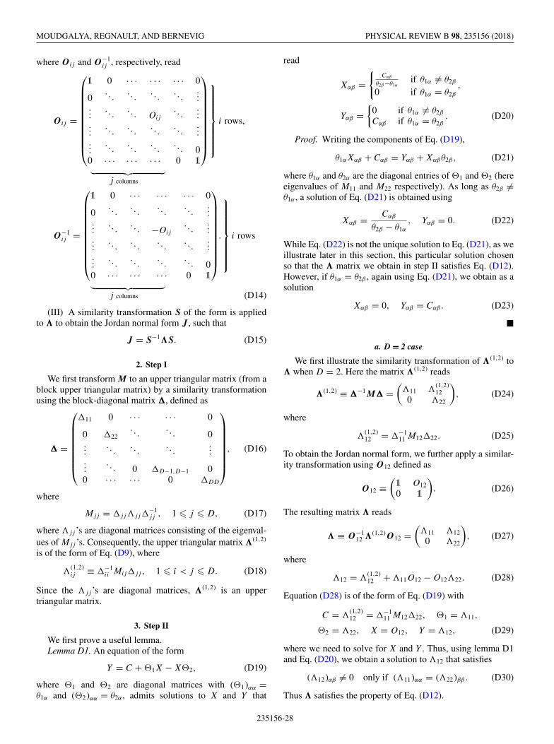
MOUDGALYA, REGNAULT, AND BERNEVIG PHYSICAL REVIEW B 98, 235156 (2018)
where O ij and O−1ij , respectively, read
O ij =
⎛⎜⎜⎜⎜⎜⎜⎜⎜⎜⎜⎝
1 0 · · · · · · · · · 0
0. . .
. . .. . .
. . ....
.... . .
. . . Oij
. . ....
.... . .
. . .. . .
. . ....
.... . .
. . .. . .
. . . 00 · · · · · · · · · 0 1
⎞⎟⎟⎟⎟⎟⎟⎟⎟⎟⎟⎠
⎫⎪⎪⎪⎪⎪⎪⎪⎬⎪⎪⎪⎪⎪⎪⎪⎭i rows,
︸ ︷︷ ︸j columns
O−1ij =
⎛⎜⎜⎜⎜⎜⎜⎜⎜⎜⎜⎝
1 0 · · · · · · · · · 0
0. . .
. . .. . .
. . ....
.... . .
. . . −Oij
. . ....
.... . .
. . .. . .
. . ....
.... . .
. . .. . .
. . . 00 · · · · · · · · · 0 1
⎞⎟⎟⎟⎟⎟⎟⎟⎟⎟⎟⎠.
⎫⎪⎪⎪⎪⎪⎪⎪⎬⎪⎪⎪⎪⎪⎪⎪⎭i rows
︸ ︷︷ ︸j columns (D14)
(III) A similarity transformation S of the form is appliedto � to obtain the Jordan normal form J , such that
J = S−1�S. (D15)
2. Step I
We first transform M to an upper triangular matrix (from ablock upper triangular matrix) by a similarity transformationusing the block-diagonal matrix �, defined as
� =
⎛⎜⎜⎜⎜⎜⎜⎜⎝
�11 0 · · · · · · 0
0 �22. . .
. . . 0...
. . .. . .
. . ....
.... . . 0 �D−1,D−1 0
0 · · · · · · 0 �DD
⎞⎟⎟⎟⎟⎟⎟⎟⎠, (D16)
where
Mjj = �jj�jj�−1jj , 1 � j � D, (D17)
where �jj ’s are diagonal matrices consisting of the eigenval-ues of Mjj ’s. Consequently, the upper triangular matrix �(1,2)
is of the form of Eq. (D9), where
�(1,2)ij ≡ �−1
ii Mij�jj , 1 � i < j � D. (D18)
Since the �jj ’s are diagonal matrices, �(1,2) is an uppertriangular matrix.
3. Step II
We first prove a useful lemma.Lemma D1. An equation of the form
Y = C + �1X − X�2, (D19)
where �1 and �2 are diagonal matrices with (�1)αα =θ1α and (�2)αα = θ2α , admits solutions to X and Y that
read
Xαβ ={
Cαβ
θ2β−θ1αif θ1α �= θ2β
0 if θ1α = θ2β
,
Yαβ ={
0 if θ1α �= θ2β
Cαβ if θ1α = θ2β. (D20)
Proof. Writing the components of Eq. (D19),
θ1αXαβ + Cαβ = Yαβ + Xαβθ2β, (D21)
where θ1α and θ2α are the diagonal entries of �1 and �2 (hereeigenvalues of M11 and M22 respectively). As long as θ2β �=θ1α , a solution of Eq. (D21) is obtained using
Xαβ = Cαβ
θ2β − θ1α
, Yαβ = 0. (D22)
While Eq. (D22) is not the unique solution to Eq. (D21), as weillustrate later in this section, this particular solution chosenso that the � matrix we obtain in step II satisfies Eq. (D12).However, if θ1α = θ2β , again using Eq. (D21), we obtain as asolution
Xαβ = 0, Yαβ = Cαβ. (D23)
�
a. D = 2 case
We first illustrate the similarity transformation of �(1,2) to� when D = 2. Here the matrix �(1,2) reads
�(1,2) ≡ �−1 M� =(
�11 �(1,2)12
0 �22
), (D24)
where
�(1,2)12 = �−1
11 M12�22. (D25)
To obtain the Jordan normal form, we further apply a similar-ity transformation using O12 defined as
O12 ≡(1 O12
0 1
). (D26)
The resulting matrix � reads
� ≡ O−112 �(1,2) O12 =
(�11 �12
0 �22
), (D27)
where
�12 = �(1,2)12 + �11O12 − O12�22. (D28)
Equation (D28) is of the form of Eq. (D19) with
C = �(1,2)12 = �−1
11 M12�22, �1 = �11,
�2 = �22, X = O12, Y = �12, (D29)
where we need to solve for X and Y . Thus, using lemma D1and Eq. (D20), we obtain a solution to �12 that satisfies
(�12)αβ �= 0 only if (�11)αα = (�22)ββ. (D30)
Thus � satisfies the property of Eq. (D12).
235156-28
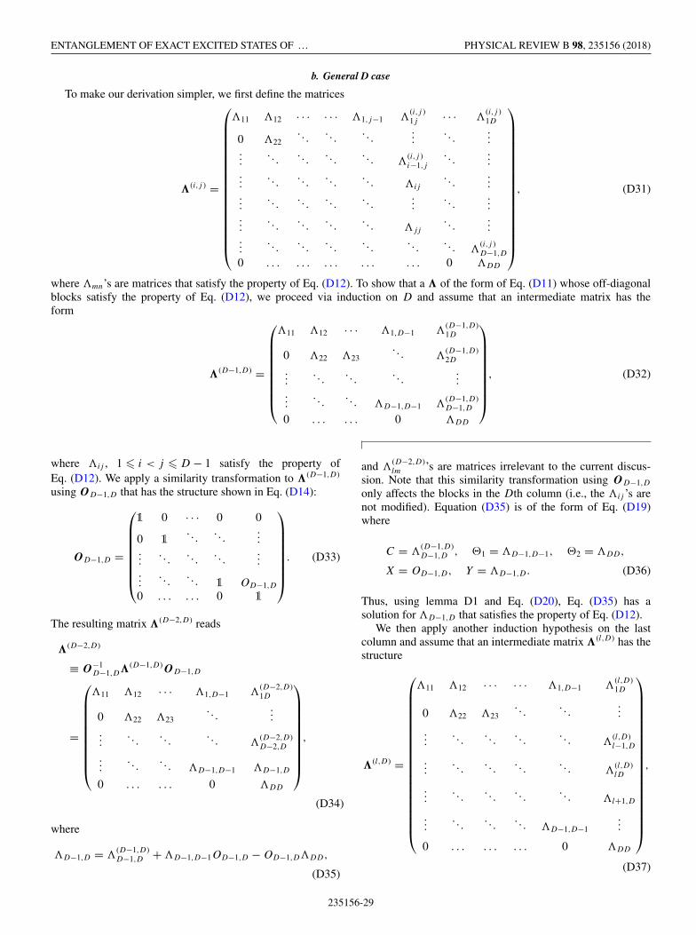
ENTANGLEMENT OF EXACT EXCITED STATES OF … PHYSICAL REVIEW B 98, 235156 (2018)
b. General D case
To make our derivation simpler, we first define the matrices
�(i,j ) =
⎛⎜⎜⎜⎜⎜⎜⎜⎜⎜⎜⎜⎜⎜⎜⎜⎜⎜⎝
�11 �12 · · · · · · �1,j−1 �(i,j )1j · · · �
(i,j )1D
0 �22. . .
. . .. . .
.... . .
......
. . .. . .
. . .. . . �
(i,j )i−1,j
. . ....
.... . .
. . .. . .
. . . �ij
. . ....
.... . .
. . .. . .
. . ....
. . ....
.... . .
. . .. . .
. . . �jj
. . ....
.... . .
. . .. . .
. . .. . .
. . . �(i,j )D−1,D
0 . . . . . . . . . . . . . . . 0 �DD
⎞⎟⎟⎟⎟⎟⎟⎟⎟⎟⎟⎟⎟⎟⎟⎟⎟⎟⎠
, (D31)
where �mn’s are matrices that satisfy the property of Eq. (D12). To show that a � of the form of Eq. (D11) whose off-diagonalblocks satisfy the property of Eq. (D12), we proceed via induction on D and assume that an intermediate matrix has theform
�(D−1,D) =
⎛⎜⎜⎜⎜⎜⎜⎜⎜⎝
�11 �12 · · · �1,D−1 �(D−1,D)1D
0 �22 �23. . . �
(D−1,D)2D
.... . .
. . .. . .
......
. . .. . . �D−1,D−1 �
(D−1,D)D−1,D
0 . . . . . . 0 �DD
⎞⎟⎟⎟⎟⎟⎟⎟⎟⎠, (D32)
where �ij , 1 � i < j � D − 1 satisfy the property ofEq. (D12). We apply a similarity transformation to �(D−1,D)
using OD−1,D that has the structure shown in Eq. (D14):
OD−1,D =
⎛⎜⎜⎜⎜⎜⎜⎜⎝
1 0 · · · 0 0
0 1. . .
. . ....
.... . .
. . .. . .
......
. . .. . . 1 OD−1,D
0 . . . . . . 0 1
⎞⎟⎟⎟⎟⎟⎟⎟⎠. (D33)
The resulting matrix �(D−2,D) reads
�(D−2,D)
≡ O−1D−1,D�(D−1,D) OD−1,D
=
⎛⎜⎜⎜⎜⎜⎜⎜⎜⎜⎝
�11 �12 · · · �1,D−1 �(D−2,D)1D
0 �22 �23. . .
......
. . .. . .
. . . �(D−2,D)D−2,D
.... . .
. . . �D−1,D−1 �D−1,D
0 . . . . . . 0 �DD
⎞⎟⎟⎟⎟⎟⎟⎟⎟⎟⎠,
(D34)
where
�D−1,D = �(D−1,D)D−1,D + �D−1,D−1OD−1,D − OD−1,D�DD,
(D35)
and �(D−2,D)lm ’s are matrices irrelevant to the current discus-
sion. Note that this similarity transformation using OD−1,D
only affects the blocks in the Dth column (i.e., the �ij ’s arenot modified). Equation (D35) is of the form of Eq. (D19)where
C = �(D−1,D)D−1,D , �1 = �D−1,D−1, �2 = �DD,
X = OD−1,D, Y = �D−1,D. (D36)
Thus, using lemma D1 and Eq. (D20), Eq. (D35) has asolution for �D−1,D that satisfies the property of Eq. (D12).
We then apply another induction hypothesis on the lastcolumn and assume that an intermediate matrix �(l,D) has thestructure
�(l,D) =
⎛⎜⎜⎜⎜⎜⎜⎜⎜⎜⎜⎜⎜⎜⎜⎜⎜⎜⎜⎜⎝
�11 �12 · · · · · · �1,D−1 �(l,D)1D
0 �22 �23. . .
. . ....
.... . .
. . .. . .
. . . �(l,D)l−1,D
.... . .
. . .. . .
. . . �(l,D)lD
.... . .
. . .. . .
. . . �l+1,D
.... . .
. . .. . . �D−1,D−1
...
0 . . . . . . . . . 0 �DD
⎞⎟⎟⎟⎟⎟⎟⎟⎟⎟⎟⎟⎟⎟⎟⎟⎟⎟⎟⎟⎠
,
(D37)
235156-29
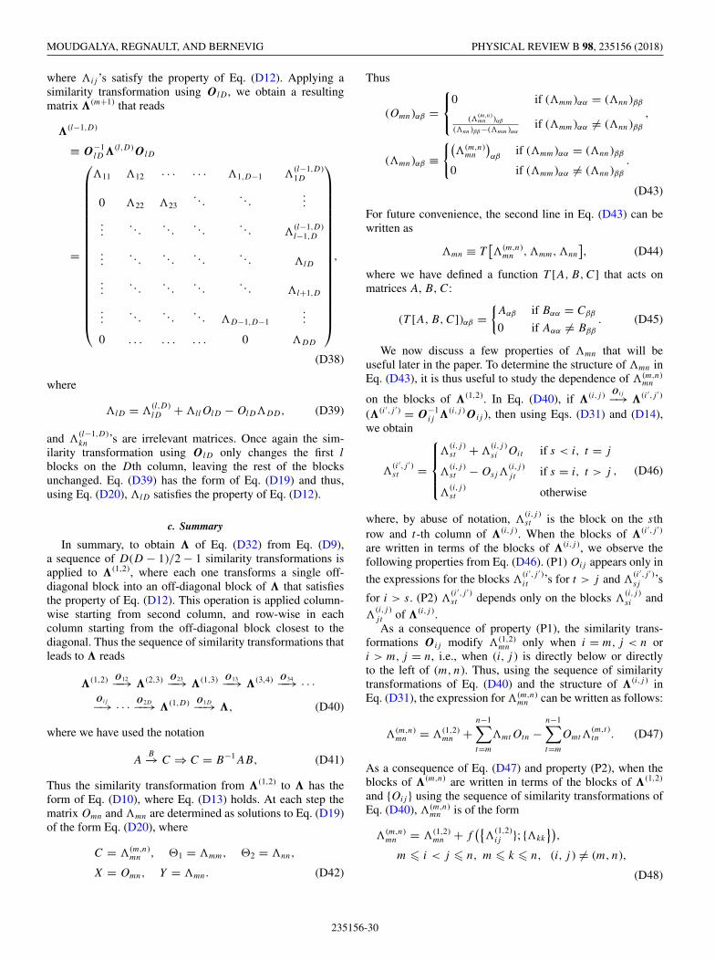
MOUDGALYA, REGNAULT, AND BERNEVIG PHYSICAL REVIEW B 98, 235156 (2018)
where �ij ’s satisfy the property of Eq. (D12). Applying asimilarity transformation using O lD , we obtain a resultingmatrix �(m+1) that reads
�(l−1,D)
≡ O−1lD �(l,D) O lD
=
⎛⎜⎜⎜⎜⎜⎜⎜⎜⎜⎜⎜⎜⎜⎜⎜⎜⎜⎜⎜⎝
�11 �12 · · · · · · �1,D−1 �(l−1,D)1D
0 �22 �23. . .
. . ....
.... . .
. . .. . .
. . . �(l−1,D)l−1,D
.... . .
. . .. . .
. . . �lD
.... . .
. . .. . .
. . . �l+1,D
.... . .
. . .. . . �D−1,D−1
...
0 . . . . . . . . . 0 �DD
⎞⎟⎟⎟⎟⎟⎟⎟⎟⎟⎟⎟⎟⎟⎟⎟⎟⎟⎟⎟⎠
,
(D38)
where
�lD = �(l,D)lD + �llOlD − OlD�DD, (D39)
and �(l−1,D)kn ’s are irrelevant matrices. Once again the sim-
ilarity transformation using O lD only changes the first l
blocks on the Dth column, leaving the rest of the blocksunchanged. Eq. (D39) has the form of Eq. (D19) and thus,using Eq. (D20), �lD satisfies the property of Eq. (D12).
c. Summary
In summary, to obtain � of Eq. (D32) from Eq. (D9),a sequence of D(D − 1)/2 − 1 similarity transformations isapplied to �(1,2), where each one transforms a single off-diagonal block into an off-diagonal block of � that satisfiesthe property of Eq. (D12). This operation is applied column-wise starting from second column, and row-wise in eachcolumn starting from the off-diagonal block closest to thediagonal. Thus the sequence of similarity transformations thatleads to � reads
�(1,2) O12−−→ �(2,3) O23−−→ �(1,3) O13−−→ �(3,4) O34−−→ · · ·O ij−→ · · · O2D−−→ �(1,D) O1D−−→ �, (D40)
where we have used the notation
AB−→ C ⇒ C = B−1AB, (D41)
Thus the similarity transformation from �(1,2) to � has theform of Eq. (D10), where Eq. (D13) holds. At each step thematrix Omn and �mn are determined as solutions to Eq. (D19)of the form Eq. (D20), where
C = �(m,n)mn , �1 = �mm, �2 = �nn,
X = Omn, Y = �mn. (D42)
Thus
(Omn)αβ =⎧⎨⎩0 if (�mm)αα = (�nn)ββ
(�(m,n)mn )αβ
(�nn )ββ−(�mm )ααif (�mm)αα �= (�nn)ββ
,
(�mn)αβ ≡{(
�(m,n)mn
)αβ
if (�mm)αα = (�nn)ββ
0 if (�mm)αα �= (�nn)ββ
.
(D43)
For future convenience, the second line in Eq. (D43) can bewritten as
�mn ≡ T[�(m,n)
mn ,�mm,�nn
], (D44)
where we have defined a function T [A,B,C] that acts onmatrices A, B, C:
(T [A,B,C])αβ ={Aαβ if Bαα = Cββ
0 if Aαα �= Bββ
. (D45)
We now discuss a few properties of �mn that will beuseful later in the paper. To determine the structure of �mn inEq. (D43), it is thus useful to study the dependence of �(m,n)
mn
on the blocks of �(1,2). In Eq. (D40), if �(i,j ) O ij−→ �(i ′,j ′ )
(�(i ′,j ′ ) = O−1ij �(i,j ) O ij ), then using Eqs. (D31) and (D14),
we obtain
�(i ′,j ′ )st =
⎧⎪⎪⎨⎪⎪⎩�
(i,j )st + �
(i,j )si Oit if s < i, t = j
�(i,j )st − Osj�
(i,j )j t if s = i, t > j
�(i,j )st otherwise
, (D46)
where, by abuse of notation, �(i,j )st is the block on the sth
row and t-th column of �(i,j ). When the blocks of �(i ′,j ′ )
are written in terms of the blocks of �(i,j ), we observe thefollowing properties from Eq. (D46). (P1) Oij appears only in
the expressions for the blocks �(i ′,j ′ )it ’s for t > j and �
(i ′,j ′ )sj ’s
for i > s. (P2) �(i ′,j ′ )st depends only on the blocks �
(i,j )si and
�(i,j )j t of �(i,j ).As a consequence of property (P1), the similarity trans-
formations O ij modify �(1,2)mn only when i = m, j < n or
i > m, j = n, i.e., when (i, j ) is directly below or directlyto the left of (m, n). Thus, using the sequence of similaritytransformations of Eq. (D40) and the structure of �(i,j ) inEq. (D31), the expression for �(m,n)
mn can be written as follows:
�(m,n)mn = �(1,2)
mn +n−1∑t=m
�mtOtn −n−1∑t=m
Omt�(m,t )tn . (D47)
As a consequence of Eq. (D47) and property (P2), when theblocks of �(m,n) are written in terms of the blocks of �(1,2)
and {Oij } using the sequence of similarity transformations ofEq. (D40), �(m,n)
mn is of the form
�(m,n)mn = �(1,2)
mn + f({
�(1,2)ij }; {�kk
}),
m � i < j � n, m � k � n, (i, j ) �= (m, n),
(D48)
235156-30
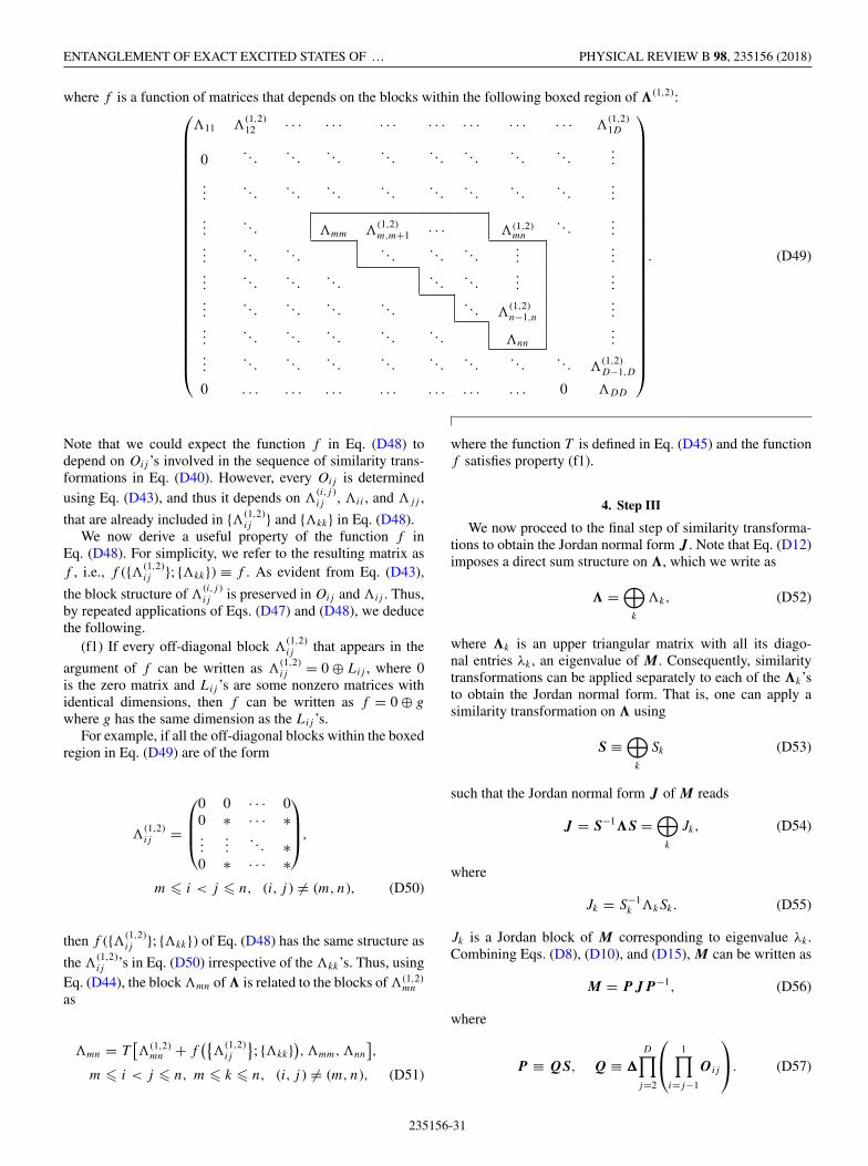
ENTANGLEMENT OF EXACT EXCITED STATES OF … PHYSICAL REVIEW B 98, 235156 (2018)
where f is a function of matrices that depends on the blocks within the following boxed region of �(1,2):⎛⎜⎜⎜⎜⎜⎜⎜⎜⎜⎜⎜⎜⎜⎜⎜⎜⎜⎜⎜⎜⎜⎜⎜⎜⎜⎜⎝
�11 �(1,2)12 · · · · · · · · · · · · · · · · · · · · · �
(1,2)1D
0. . .
. . .. . .
. . .. . .
. . .. . .
. . ....
.... . .
. . .. . .
. . .. . .
. . .. . .
. . ....
.... . . �mm �
(1,2)m,m+1 · · · �(1,2)
mn
. . ....
.... . .
. . .. . .
. . .. . .
......
.... . .
. . .. . .
. . .. . .
......
.... . .
. . .. . .
. . .. . . �
(1,2)n−1,n
......
. . .. . .
. . .. . .
. . . �nn
......
. . .. . .
. . .. . .
. . .. . .
. . .. . . �
(1,2)D−1,D
0 . . . . . . . . . . . . . . . . . . . . . 0 �DD
⎞⎟⎟⎟⎟⎟⎟⎟⎟⎟⎟⎟⎟⎟⎟⎟⎟⎟⎟⎟⎟⎟⎟⎟⎟⎟⎟⎠
. (D49)
Note that we could expect the function f in Eq. (D48) todepend on Oij ’s involved in the sequence of similarity trans-formations in Eq. (D40). However, every Oij is determinedusing Eq. (D43), and thus it depends on �
(i,j )ij , �ii , and �jj ,
that are already included in {�(1,2)ij } and {�kk} in Eq. (D48).
We now derive a useful property of the function f inEq. (D48). For simplicity, we refer to the resulting matrix asf , i.e., f ({�(1,2)
ij }; {�kk}) ≡ f . As evident from Eq. (D43),
the block structure of �(i,j )ij is preserved in Oij and �ij . Thus,
by repeated applications of Eqs. (D47) and (D48), we deducethe following.
(f1) If every off-diagonal block �(1,2)ij that appears in the
argument of f can be written as �(1,2)ij = 0 ⊕ Lij , where 0
is the zero matrix and Lij ’s are some nonzero matrices withidentical dimensions, then f can be written as f = 0 ⊕ g
where g has the same dimension as the Lij ’s.For example, if all the off-diagonal blocks within the boxed
region in Eq. (D49) are of the form
�(1,2)ij =
⎛⎜⎜⎝0 0 · · · 00 ∗ · · · ∗...
.... . . ∗
0 ∗ · · · ∗
⎞⎟⎟⎠,
m � i < j � n, (i, j ) �= (m, n), (D50)
then f ({�(1,2)ij }; {�kk}) of Eq. (D48) has the same structure as
the �(1,2)ij ’s in Eq. (D50) irrespective of the �kk’s. Thus, using
Eq. (D44), the block �mn of � is related to the blocks of �(1,2)mn
as
�mn = T[�(1,2)
mn + f({
�(1,2)ij
}; {�kk}
),�mm,�nn
],
m � i < j � n, m � k � n, (i, j ) �= (m, n), (D51)
where the function T is defined in Eq. (D45) and the functionf satisfies property (f1).
4. Step III
We now proceed to the final step of similarity transforma-tions to obtain the Jordan normal form J . Note that Eq. (D12)imposes a direct sum structure on �, which we write as
� =⊕
k
�k, (D52)
where �k is an upper triangular matrix with all its diago-nal entries λk , an eigenvalue of M. Consequently, similaritytransformations can be applied separately to each of the �k’sto obtain the Jordan normal form. That is, one can apply asimilarity transformation on � using
S ≡⊕
k
Sk (D53)
such that the Jordan normal form J of M reads
J = S−1�S =⊕
k
Jk, (D54)
where
Jk = S−1k �kSk. (D55)
Jk is a Jordan block of M corresponding to eigenvalue λk .Combining Eqs. (D8), (D10), and (D15), M can be written as
M = P J P−1, (D56)
where
P ≡ QS, Q ≡ �
D∏j=2
⎛⎝ 1∏i=j−1
O ij
⎞⎠. (D57)
235156-31

MOUDGALYA, REGNAULT, AND BERNEVIG PHYSICAL REVIEW B 98, 235156 (2018)
Using Eqs. (D8), (D16), (D14), and (D57), Q and Q−1 read
Q = �
D∏j=2
1∏i=j−1
O ij
=
⎛⎜⎜⎜⎜⎜⎜⎜⎝
�11 ∗ · · · · · · ∗0 �22
. . .. . . ∗
.... . .
. . .. . .
......
. . . 0 �D−1,D−1 ∗0 · · · · · · 0 �DD
⎞⎟⎟⎟⎟⎟⎟⎟⎠,
Q−1 =2∏
j=D
j−1∏i=1
O−1ij �−1
=
⎛⎜⎜⎜⎜⎜⎜⎜⎝
�−111 ∗ · · · · · · ∗0 �−1
22
. . .. . . ∗
.... . .
. . .. . .
......
. . . 0 �−1D−1,D−1 ∗
0 · · · · · · 0 �−1DD
⎞⎟⎟⎟⎟⎟⎟⎟⎠, (D58)
where ∗’s are matrices whose structure we will not need forthe discussion in the main text.
5. Structure of generalized eigenvectors
We now study the columns (respectively, rows) of P (re-spectively, P−1) that are the generalized eigenvectors corre-sponding to the generalized eigenvalues of unit magnitude.For �, S, J , it is convenient to write Eqs. (D52)–(D54) as
� = �unit ⊕ �rest, S = Sunit ⊕ Srest, J = Junit ⊕ Jrest,
(D59)
where
�unit =⊕
{k:|λk |=1}�k, �rest =
⊕{k:|λk |�=1}
�k,
Sunit =⊕
{k:|λk |=1}Sk, Srest =
⊕{k:|λk |�=1}
Sk, (D60)
Junit =⊕
{k:|λk |=1}Jk, Jrest =
⊕{k:|λk |�=1}
Jk.
Indeed, only the generalized eigenvalues of magnitude oneare relevant in our case and we have assumed that each Mii
has at most one such eigenvalue (note that this does not meanthat these eigenvalues are identical). Since � has a direct sumstructure shown in Eq. (D59), M can be written as
M = Qunit�unitQunit + Qrest�restQrest, (D61)
where Qunit, Qunit, Qrest, and Qrest are rectangular matricessuch that the columns (respectively, rows) of Qunit (respec-tively, Qunit) and Qrest (respectively, Qrest) act on the sub-spaces of �unit and �rest, respectively.
Since � has the structure shown in Eq. (D11) and onlythe blocks Mσ (i),σ (i) (and consequently �σ (i),σ (i)), 1 � i � d
contain eigenvalues of magnitude 1, using Eq. (D58) Qunit andQunit have d rows and columns, respectively, and are of the
forms
Qunit = (qσ (1) qσ (2) · · · qσ (d ) ), Qunit =
⎛⎜⎜⎜⎝qσ (1)
qσ (2)...
qσ (d )
⎞⎟⎟⎟⎠,
(D62)
where
qσ (i) =
⎛⎜⎜⎜⎜⎜⎜⎜⎜⎜⎝
∗...∗
rσ (i)
0...0
⎞⎟⎟⎟⎟⎟⎟⎟⎟⎟⎠
⎫⎪⎬⎪⎭ σ (i) − 1,
qσ (i) = (0 · · · 0 lTσ (i) ∗ · · · ∗ )︸ ︷︷ ︸
d−σ (i)+1
(D63)
where {rj } (respectively, {lj }) are right (respectively, left) gen-eralized eigenvectors of {Mjj } corresponding to the general-ized eigenvalues of unit magnitude. Further, using Eqs. (D55)and (D61) can be written as
M = PunitJunitPunit + PrestJrestPrest, (D64)
where
Punit ≡ QunitSunit, Punit ≡ S−1unitQunit,
Prest ≡ QrestSrest, Prest ≡ S−1restQrest. (D65)
Since Qunit and Qunit have the forms shown in Eqs. (D62)and (D63), using Eq. (D65), we obtain that
Punit = (sσ (1)qσ (1) sσ (2)qσ (2) · · · sσ (d )qσ (d ) ),
Punit =
⎛⎜⎜⎜⎜⎜⎝qσ (1)
sσ (1)
qσ (2)
sσ (2)
...qσ (d )
sσ (d )
⎞⎟⎟⎟⎟⎟⎠,
if Sunit is upper triangular and has the form
Sunit =
⎛⎜⎜⎜⎜⎜⎜⎜⎝
sσ (1) ∗ · · · · · · ∗0 sσ (2)
. . .. . . ∗
.... . .
. . .. . .
......
. . . 0 sσ (d−1) ∗0 · · · · · · 0 sσ (d )
⎞⎟⎟⎟⎟⎟⎟⎟⎠, (D66)
where the si’s are nonzero constants. Thus, when Sunit is uppertriangular with all nonzero diagonal entries on its diagonal,the left and right generalized eigenvectors corresponding togeneralized eigenvalues of unit magnitude have the following
235156-32
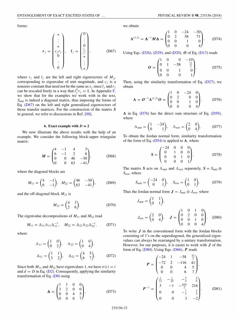
ENTANGLEMENT OF EXACT EXCITED STATES OF … PHYSICAL REVIEW B 98, 235156 (2018)
forms:
rj =
⎛⎜⎜⎜⎜⎜⎜⎜⎜⎜⎝
∗...∗
cj rj
0...0
⎞⎟⎟⎟⎟⎟⎟⎟⎟⎟⎠, lj =
⎛⎜⎜⎜⎜⎜⎜⎜⎜⎜⎜⎝
0...0ljcj
∗...∗
⎞⎟⎟⎟⎟⎟⎟⎟⎟⎟⎟⎠, (D67)
where rj and lj are the left and right eigenvectors of Mjj
corresponding to eigenvalue of unit magnitude, and cj is anonzero constant that need not be the same as sj since lj and rj
can be rescaled freely in a way that lTj rj = 1. In Appendix F,we show that for the examples we work with in the text,Sunit is indeed a diagonal matrix, thus imposing the forms ofEq. (D67) on the left and right generalized eigenvectors ofthose transfer matrices. For the construction of the matrix Sin general, we refer to discussions in Ref. [98].
6. Exact example with D = 2
We now illustrate the above results with the help of anexample. We consider the following block-upper triangularmatrix:
M =
⎛⎜⎝4 −1 4 36 −1 2 60 0 46 −300 0 63 −41
⎞⎟⎠, (D68)
where the diagonal blocks are
M11 =(
4 −16 −1
), M22 =
(46 −3063 −41
), (D69)
and the off-diagonal block M12 is
M12 =(
4 32 6
). (D70)
The eigenvalue decompositions of M11 and M22 read
M11 = �11�11�−111 , M22 = �22�22�
−122 , (D71)
where
�11 =(
1 00 2
), �22 =
(1 00 4
),
�11 =(
1 13 2
), �22 =
(4 56 7
). (D72)
Since both M11 and M22 have eigenvalues 1, we have σ (i) = i
and d = D in Eq. (D2). Consequently, applying the similaritytransformation of Eq. (D8) using
� =
⎛⎜⎝1 1 0 03 2 0 00 0 4 50 0 6 7
⎞⎟⎠, (D73)
we obtain
�(1,2) = �−1 M� =
⎛⎜⎝1 0 −24 −300 2 58 710 0 1 00 0 0 4
⎞⎟⎠. (D74)
Using Eqs. (D26), (D29), and (D20), O of Eq. (D13) reads
O =
⎛⎜⎜⎝1 0 0 −100 1 −58 71
2
0 0 1 00 0 0 1
⎞⎟⎟⎠. (D75)
Then, using the similarity transformation of Eq. (D27), weobtain
� = O−1�(1,2) O =
⎛⎜⎝1 0 −24 00 2 0 00 0 1 00 0 0 4
⎞⎟⎠. (D76)
� in Eq. (D76) has the direct sum structure of Eq. (D59),where
�unit =(
1 −240 1
), �rest =
(2 00 4
). (D77)
To obtain the Jordan normal form, similarity transformationof the form of Eq. (D54) is applied to �, where
S =
⎛⎜⎝−24 0 0 00 1 0 00 0 1 00 0 0 1
⎞⎟⎠. (D78)
The matrix S acts on �unit and �rest separately, S = Sunit ⊕Srest, where
Sunit =(−24 0
0 1
), Srest =
(1 00 1
). (D79)
Thus the Jordan normal form J = Junit ⊕ Jrest, where
Junit =(
1 10 1
),
Jrest =(
2 00 4
), J =
⎛⎜⎝1 0 1 00 2 0 00 0 1 00 0 0 4
⎞⎟⎠. (D80)
To write J in the conventional form with the Jordan blocksconsisting of 1’s on the superdiagonal, the generalized eigen-values can always be rearranged by a unitary transformation.However, for our purposes, it is easier to work with J of theform of Eq. (D80). Using Eqs. (D66), P reads
P =
⎛⎜⎜⎝−24 1 −58 51
2
−72 2 −116 410 0 4 50 0 6 7
⎞⎟⎟⎠,
P−1 =
⎛⎜⎜⎜⎜⎝1
12 − 124 − 5
456
3 −1 − 6192 216
0 0 − 72
52
0 0 3 −2
⎞⎟⎟⎟⎟⎠. (D81)
235156-33
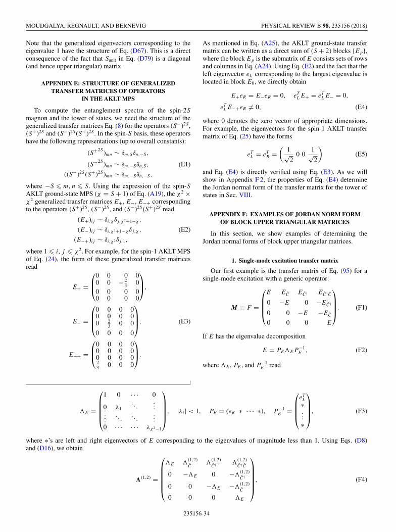
MOUDGALYA, REGNAULT, AND BERNEVIG PHYSICAL REVIEW B 98, 235156 (2018)
Note that the generalized eigenvectors corresponding to theeigenvalue 1 have the structure of Eq. (D67). This is a directconsequence of the fact that Sunit in Eq. (D79) is a diagonal(and hence upper triangular) matrix.
APPENDIX E: STRUCTURE OF GENERALIZEDTRANSFER MATRICES OF OPERATORS
IN THE AKLT MPS
To compute the entanglement spectra of the spin-2S
magnon and the tower of states, we need the structure of thegeneralized transfer matrices Eq. (8) for the operators (S−)2S ,(S+)2S and (S−)2S (S+)2S . In the spin-S basis, these operatorshave the following representations (up to overall constants):
(S+2S )mn ∼ δm,Sδn,−S,
(S−2S )mn ∼ δm,−Sδn,S, (E1)
((S−)2S (S+)2S )mn ∼ δm,−Sδn,−S,
where −S � m, n � S. Using the expression of the spin-SAKLT ground-state MPS (χ = S + 1) of Eq. (A19), the χ2 ×χ2 generalized transfer matrices E+, E−, E−+ correspondingto the operators (S+)2S , (S−)2S , and (S−)2S (S+)2S read
(E+)ij ∼ δi,χ δj,χ2+1−χ ,
(E−)ij ∼ δi,χ2+1−χδj,χ , (E2)
(E−+)ij ∼ δi,χ2δj,1,
where 1 � i, j � χ2. For example, for the spin-1 AKLT MPSof Eq. (24), the form of these generalized transfer matricesread
E+ =
⎛⎜⎝0 0 0 00 0 − 2
3 00 0 0 00 0 0 0
⎞⎟⎠,
E− =
⎛⎜⎜⎝0 0 0 00 0 0 00 2
3 0 0
0 0 0 0
⎞⎟⎟⎠, (E3)
E−+ =
⎛⎜⎝0 0 0 00 0 0 00 0 0 023 0 0 0
⎞⎟⎠.
As mentioned in Eq. (A25), the AKLT ground-state transfermatrix can be written as a direct sum of (S + 2) blocks {Ep},where the block Ep is the submatrix of E consists sets of rowsand columns in Eq. (A24). Using Eq. (E2) and the fact that theleft eigenvector eL corresponding to the largest eigenvalue islocated in block E0, we directly obtain
E+eR = E−eR = 0, eTLE+ = eT
LE− = 0,
eTLE−+eR �= 0, (E4)
where 0 denotes the zero vector of appropriate dimensions.For example, the eigenvectors for the spin-1 AKLT transfermatrix of Eq. (25) have the forms
eTL = eT
R =(
1√2
0 01√2
)(E5)
and Eq. (E4) is directly verified using Eq. (E3). As we willshow in Appendix F 2, the properties of Eq. (E4) determinethe Jordan normal form of the transfer matrix for the tower ofstates in Sec. VIII.
APPENDIX F: EXAMPLES OF JORDAN NORM FORMOF BLOCK UPPER TRIANGULAR MATRICES
In this section, we show examples of determining theJordan normal forms of block upper triangular matrices.
1. Single-mode excitation transfer matrix
Our first example is the transfer matrix of Eq. (95) for asingle-mode excitation with a generic operator:
M ≡ F =
⎛⎜⎜⎜⎝E EC EC† EC†C
0 −E 0 −EC†
0 0 −E −EC
0 0 0 E
⎞⎟⎟⎟⎠. (F1)
If E has the eigenvalue decomposition
E = PE�EP −1E , (F2)
where �E , PE , and P −1E read
�E =
⎛⎜⎜⎜⎜⎝1 0 · · · 0
0 λ1. . .
......
. . .. . .
...0 · · · · · · λχ2−1
⎞⎟⎟⎟⎟⎠, |λi | < 1, PE = (eR ∗ · · · ∗), P −1E =
⎛⎜⎜⎜⎝eTL∗...∗
⎞⎟⎟⎟⎠, (F3)
where ∗’s are left and right eigenvectors of E corresponding to the eigenvalues of magnitude less than 1. Using Eqs. (D8)and (D16), we obtain
�(1,2) =
⎛⎜⎜⎜⎜⎜⎝�E �
(1,2)C
�(1,2)C† �
(1,2)C†C
0 −�E 0 −�(1,2)C†
0 0 −�E −�(1,2)C
0 0 0 �E
⎞⎟⎟⎟⎟⎟⎠, (F4)
235156-34
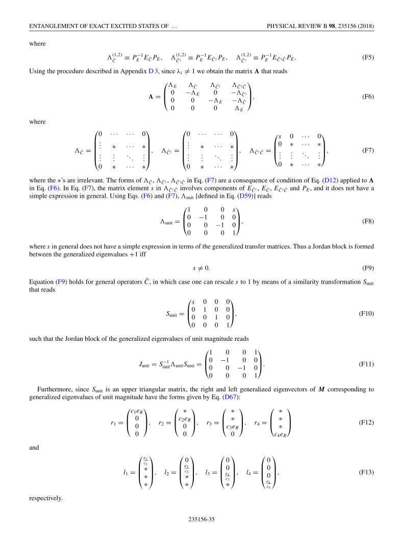
ENTANGLEMENT OF EXACT EXCITED STATES OF … PHYSICAL REVIEW B 98, 235156 (2018)
where
�(1,2)C
≡ P −1E ECPE, �
(1,2)C† ≡ P −1
E EC†PE, �(1,2)C† ≡ P −1
E EC†CPE. (F5)
Using the procedure described in Appendix D 3, since λi �= 1 we obtain the matrix � that reads
� =
⎛⎜⎝�E �C �C† �C†C0 −�E 0 −�C†
0 0 −�E −�C
0 0 0 �E
⎞⎟⎠, (F6)
where
�C =
⎛⎜⎜⎜⎜⎝0 · · · · · · 0... ∗ · · · ∗...
.... . .
...0 ∗ · · · ∗
⎞⎟⎟⎟⎟⎠, �C† =
⎛⎜⎜⎜⎜⎝0 · · · · · · 0... ∗ · · · ∗...
.... . .
...0 ∗ · · · ∗
⎞⎟⎟⎟⎟⎠, �C†C =
⎛⎜⎜⎝s 0 · · · 00 ∗ · · · ∗...
.... . .
...0 ∗ · · · ∗
⎞⎟⎟⎠, (F7)
where the ∗’s are irrelevant. The forms of �C , �C† , �C†C in Eq. (F7) are a consequence of condition of Eq. (D12) applied to �
in Eq. (F6). In Eq. (F7), the matrix element s in �C†C involves components of EC† , EC , EC†C and PE , and it does not have asimple expression in general. Using Eqs. (F6) and (F7), �unit [defined in Eq. (D59)] reads
�unit =
⎛⎜⎝1 0 0 s
0 −1 0 00 0 −1 00 0 0 1
⎞⎟⎠, (F8)
where s in general does not have a simple expression in terms of the generalized transfer matrices. Thus a Jordan block is formedbetween the generalized eigenvalues +1 iff
s �= 0. (F9)
Equation (F9) holds for general operators C, in which case one can rescale s to 1 by means of a similarity transformation Sunit
that reads
Sunit =
⎛⎜⎝s 0 0 00 1 0 00 0 1 00 0 0 1
⎞⎟⎠, (F10)
such that the Jordan block of the generalized eigenvalues of unit magnitude reads
Junit = S−1unit�unitSunit =
⎛⎜⎝1 0 0 10 −1 0 00 0 −1 00 0 0 1
⎞⎟⎠. (F11)
Furthermore, since Sunit is an upper triangular matrix, the right and left generalized eigenvectors of M corresponding togeneralized eigenvalues of unit magnitude have the forms given by Eq. (D67):
r1 =
⎛⎜⎝c1eR
000
⎞⎟⎠, r2 =
⎛⎜⎝ ∗c2eR
00
⎞⎟⎠, r3 =
⎛⎜⎝ ∗∗
c3eR
0
⎞⎟⎠, r4 =
⎛⎜⎝ ∗∗∗
c4eR
⎞⎟⎠ (F12)
and
l1 =
⎛⎜⎜⎝eL
c1∗∗∗
⎞⎟⎟⎠, l2 =
⎛⎜⎜⎝0eL
c2∗∗
⎞⎟⎟⎠, l3 =
⎛⎜⎜⎝00eL
c3∗
⎞⎟⎟⎠, l4 =
⎛⎜⎜⎝000eL
c4
⎞⎟⎟⎠, (F13)
respectively.
235156-35
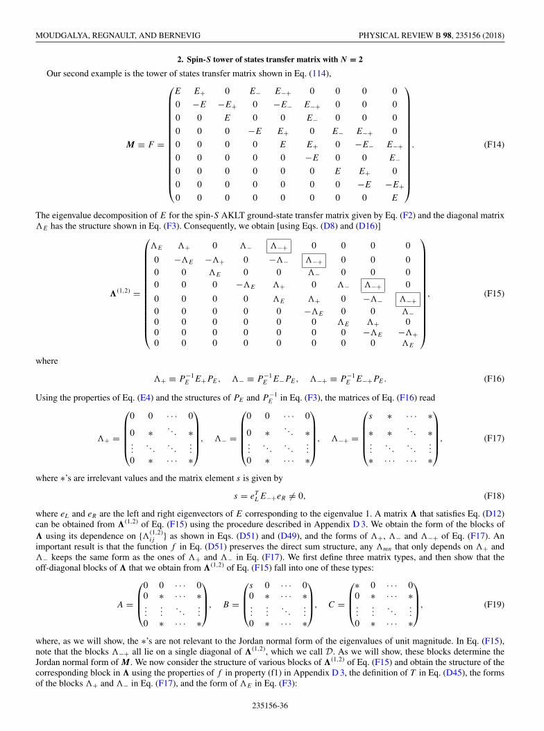
MOUDGALYA, REGNAULT, AND BERNEVIG PHYSICAL REVIEW B 98, 235156 (2018)
2. Spin-S tower of states transfer matrix with N = 2
Our second example is the tower of states transfer matrix shown in Eq. (114),
M ≡ F =
⎛⎜⎜⎜⎜⎜⎜⎜⎜⎜⎜⎜⎜⎜⎜⎜⎝
E E+ 0 E− E−+ 0 0 0 0
0 −E −E+ 0 −E− E−+ 0 0 0
0 0 E 0 0 E− 0 0 0
0 0 0 −E E+ 0 E− E−+ 0
0 0 0 0 E E+ 0 −E− E−+0 0 0 0 0 −E 0 0 E−0 0 0 0 0 0 E E+ 0
0 0 0 0 0 0 0 −E −E+0 0 0 0 0 0 0 0 E
⎞⎟⎟⎟⎟⎟⎟⎟⎟⎟⎟⎟⎟⎟⎟⎟⎠. (F14)
The eigenvalue decomposition of E for the spin-S AKLT ground-state transfer matrix given by Eq. (F2) and the diagonal matrix�E has the structure shown in Eq. (F3). Consequently, we obtain [using Eqs. (D8) and (D16)]
�(1,2) =
⎛⎜⎜⎜⎜⎜⎜⎜⎜⎜⎜⎜⎜⎜⎜⎝
�E �+ 0 �− �−+ 0 0 0 0
0 −�E −�+ 0 −�− �−+ 0 0 00 0 �E 0 0 �− 0 0 00 0 0 −�E �+ 0 �− �−+ 0
0 0 0 0 �E �+ 0 −�− �−+0 0 0 0 0 −�E 0 0 �−0 0 0 0 0 0 �E �+ 00 0 0 0 0 0 0 −�E −�+0 0 0 0 0 0 0 0 �E
⎞⎟⎟⎟⎟⎟⎟⎟⎟⎟⎟⎟⎟⎟⎟⎠, (F15)
where
�+ ≡ P −1E E+PE, �− ≡ P −1
E E−PE, �−+ ≡ P −1E E−+PE. (F16)
Using the properties of Eq. (E4) and the structures of PE and P −1E in Eq. (F3), the matrices of Eq. (F16) read
�+ =
⎛⎜⎜⎜⎜⎝0 0 · · · 0
0 ∗ . . . ∗...
. . .. . .
...0 ∗ · · · ∗
⎞⎟⎟⎟⎟⎠, �− =
⎛⎜⎜⎜⎜⎝0 0 · · · 0
0 ∗ . . . ∗...
. . .. . .
...0 ∗ · · · ∗
⎞⎟⎟⎟⎟⎠, �−+ =
⎛⎜⎜⎜⎜⎝s ∗ · · · ∗∗ ∗ . . . ∗...
. . .. . .
...∗ · · · · · · ∗
⎞⎟⎟⎟⎟⎠, (F17)
where ∗’s are irrelevant values and the matrix element s is given by
s = eTLE−+eR �= 0, (F18)
where eL and eR are the left and right eigenvectors of E corresponding to the eigenvalue 1. A matrix � that satisfies Eq. (D12)can be obtained from �(1,2) of Eq. (F15) using the procedure described in Appendix D 3. We obtain the form of the blocks of� using its dependence on {�(1,2)
ij } as shown in Eqs. (D51) and (D49), and the forms of �+, �− and �−+ of Eq. (F17). Animportant result is that the function f in Eq. (D51) preserves the direct sum structure, any �mn that only depends on �+ and�− keeps the same form as the ones of �+ and �− in Eq. (F17). We first define three matrix types, and then show that theoff-diagonal blocks of � that we obtain from �(1,2) of Eq. (F15) fall into one of these types:
A =
⎛⎜⎜⎝0 0 · · · 00 ∗ · · · ∗...
.... . .
...0 ∗ · · · ∗
⎞⎟⎟⎠, B =
⎛⎜⎜⎝s 0 · · · 00 ∗ · · · ∗...
.... . .
...0 ∗ · · · ∗
⎞⎟⎟⎠, C =
⎛⎜⎜⎝∗ 0 · · · 00 ∗ · · · ∗...
.... . .
...0 ∗ · · · ∗
⎞⎟⎟⎠, (F19)
where, as we will show, the ∗’s are not relevant to the Jordan normal form of the eigenvalues of unit magnitude. In Eq. (F15),note that the blocks �−+ all lie on a single diagonal of �(1,2), which we call D. As we will show, these blocks determine theJordan normal form of M. We now consider the structure of various blocks of �(1,2) of Eq. (F15) and obtain the structure of thecorresponding block in � using the properties of f in property (f1) in Appendix D 3, the definition of T in Eq. (D45), the formsof the blocks �+ and �− in Eq. (F17), and the form of �E in Eq. (F3):
235156-36
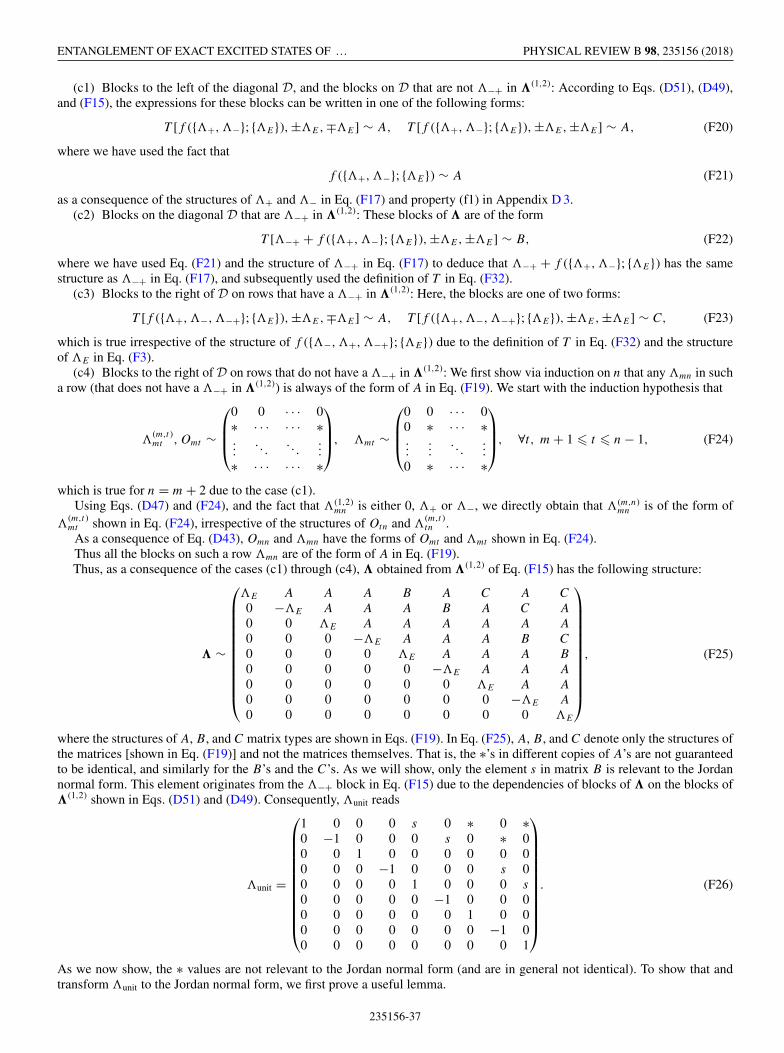
ENTANGLEMENT OF EXACT EXCITED STATES OF … PHYSICAL REVIEW B 98, 235156 (2018)
(c1) Blocks to the left of the diagonal D, and the blocks on D that are not �−+ in �(1,2): According to Eqs. (D51), (D49),and (F15), the expressions for these blocks can be written in one of the following forms:
T [f ({�+,�−}; {�E}),±�E,∓�E] ∼ A, T [f ({�+,�−}; {�E}),±�E,±�E] ∼ A, (F20)
where we have used the fact that
f ({�+,�−}; {�E}) ∼ A (F21)
as a consequence of the structures of �+ and �− in Eq. (F17) and property (f1) in Appendix D 3.(c2) Blocks on the diagonal D that are �−+ in �(1,2): These blocks of � are of the form
T [�−+ + f ({�+,�−}; {�E}),±�E,±�E] ∼ B, (F22)
where we have used Eq. (F21) and the structure of �−+ in Eq. (F17) to deduce that �−+ + f ({�+,�−}; {�E}) has the samestructure as �−+ in Eq. (F17), and subsequently used the definition of T in Eq. (F32).
(c3) Blocks to the right of D on rows that have a �−+ in �(1,2): Here, the blocks are one of two forms:
T [f ({�+,�−,�−+}; {�E}),±�E,∓�E] ∼ A, T [f ({�+,�−,�−+}; {�E}),±�E,±�E] ∼ C, (F23)
which is true irrespective of the structure of f ({�−,�+,�−+}; {�E}) due to the definition of T in Eq. (F32) and the structureof �E in Eq. (F3).
(c4) Blocks to the right of D on rows that do not have a �−+ in �(1,2): We first show via induction on n that any �mn in sucha row (that does not have a �−+ in �(1,2)) is always of the form of A in Eq. (F19). We start with the induction hypothesis that
�(m,t )mt ,Omt ∼
⎛⎜⎜⎝0 0 · · · 0∗ · · · · · · ∗...
. . .. . .
...∗ · · · · · · ∗
⎞⎟⎟⎠, �mt ∼
⎛⎜⎜⎝0 0 · · · 00 ∗ · · · ∗...
.... . .
...0 ∗ · · · ∗
⎞⎟⎟⎠, ∀t, m + 1 � t � n − 1, (F24)
which is true for n = m + 2 due to the case (c1).Using Eqs. (D47) and (F24), and the fact that �(1,2)
mn is either 0, �+ or �−, we directly obtain that �(m,n)mn is of the form of
�(m,t )mt shown in Eq. (F24), irrespective of the structures of Otn and �
(m,t )tn .
As a consequence of Eq. (D43), Omn and �mn have the forms of Omt and �mt shown in Eq. (F24).Thus all the blocks on such a row �mn are of the form of A in Eq. (F19).Thus, as a consequence of the cases (c1) through (c4), � obtained from �(1,2) of Eq. (F15) has the following structure:
� ∼
⎛⎜⎜⎜⎜⎜⎜⎜⎜⎜⎜⎜⎝
�E A A A B A C A C
0 −�E A A A B A C A
0 0 �E A A A A A A
0 0 0 −�E A A A B C
0 0 0 0 �E A A A B
0 0 0 0 0 −�E A A A
0 0 0 0 0 0 �E A A
0 0 0 0 0 0 0 −�E A
0 0 0 0 0 0 0 0 �E
⎞⎟⎟⎟⎟⎟⎟⎟⎟⎟⎟⎟⎠, (F25)
where the structures of A, B, and C matrix types are shown in Eqs. (F19). In Eq. (F25), A, B, and C denote only the structures ofthe matrices [shown in Eq. (F19)] and not the matrices themselves. That is, the ∗’s in different copies of A’s are not guaranteedto be identical, and similarly for the B’s and the C’s. As we will show, only the element s in matrix B is relevant to the Jordannormal form. This element originates from the �−+ block in Eq. (F15) due to the dependencies of blocks of � on the blocks of�(1,2) shown in Eqs. (D51) and (D49). Consequently, �unit reads
�unit =
⎛⎜⎜⎜⎜⎜⎜⎜⎜⎜⎜⎜⎝
1 0 0 0 s 0 ∗ 0 ∗0 −1 0 0 0 s 0 ∗ 00 0 1 0 0 0 0 0 00 0 0 −1 0 0 0 s 00 0 0 0 1 0 0 0 s
0 0 0 0 0 −1 0 0 00 0 0 0 0 0 1 0 00 0 0 0 0 0 0 −1 00 0 0 0 0 0 0 0 1
⎞⎟⎟⎟⎟⎟⎟⎟⎟⎟⎟⎟⎠. (F26)
As we now show, the ∗ values are not relevant to the Jordan normal form (and are in general not identical). To show that andtransform �unit to the Jordan normal form, we first prove a useful lemma.
235156-37
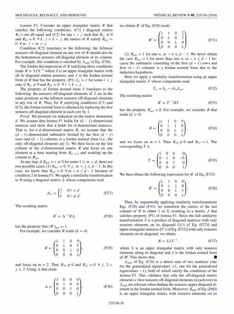
MOUDGALYA, REGNAULT, AND BERNEVIG PHYSICAL REVIEW B 98, 235156 (2018)
Lemma F1. Consider an upper triangular matrix R thatsatisfies the following conditions: (C1) t diagonal entriesRii’s are all equal and (C2) for any i < j such that Rij �= 0and Rik = 0 ∀ k, i < k < j , the entries of R satisfy Rmj =0 ∀ m, i < m < j .
Condition (C2) translates to the following: the leftmostnonzero off-diagonal element on any row of R should also bethe bottommost nonzero off-diagonal element of its column.For example, this condition is satisfied by �unit of Eq. (F26).
The Jordan decomposition of R satisfying these conditionsreads R = SJS−1 where S is an upper triangular matrix withall its diagonal entries nonzero, and J is the Jordan normalform of R that has the property: (P1) Jij = 1 for some i < j
only if Rij �= 0 and Rik = 0 ∀ i < k < j .The property of Jordan normal form J translates to the
following: the nonzero off-diagonal elements of J are in thesame positions as the leftmost nonzero off-diagonal elementsin any row of R. Thus, for R satisfying conditions (C1) and(C2), the Jordan normal form is obtained by replacing the firstnonzero off-diagonal element in each row by 1.
Proof. We proceed via induction on the matrix dimensiond. We assume that lemma F1 holds for (d − 1)-dimensionalmatrices and show that it holds for d-dimensional matrices.That is, for a d-dimensional matrix R, we assume that the(d − 1)-dimensional submatrix formed by the first (d − 1)rows and (d − 1) columns is a Jordan normal form (i.e., theonly off-diagonal elements are 1). We then focus on the lastcolumn of the d-dimensional matrix R and focus on oneelement at a time starting from Rd−1,d and working up thecolumn to R1d .
At any step, if Rmd = t �= 0 for some 1 � m < d, there aretwo possible cases: (1) Rmj = 0 ∀ j, m < j � d − 1. In thiscase, we know that Rnd = 0 ∀ m < n < d − 1 because ofcondition 2 in lemma F1. We apply a similarity transformationto R using a diagonal matrix � whose components read
�ii ={ 1
tif i = d
1 if i �= d. (F27)
The resulting matrix
R′ = �−1R� (F28)
has the property that (R′)md = 1.For example, we consider R reads (d = 4)
R =
⎛⎜⎝λ 1 0 50 λ 0 20 0 λ 00 0 0 λ
⎞⎟⎠, (F29)
and focus on m = 2. Thus R24 �= 0 and R2j = 0 ∀ j, 2 <
j � 3. Using � that reads
� =
⎛⎜⎜⎝1 0 0 00 1 0 00 0 1 00 0 0 1
2
⎞⎟⎟⎠, (F30)
we obtain R′ of Eq. (F28) reads
R′ =
⎛⎜⎜⎝λ 1 0 5
20 λ 0 10 0 λ 00 0 0 λ
⎞⎟⎟⎠. (F31)
(2) Rmn = 1 for one n, m < n � d − 1. We never obtainthe case Rmn = 1 for more than one n, m < n � d − 1 be-cause the submatrix consisting of the first (d − 1) rows andfirst (d − 1) columns is a Jordan normal form due to theinduction hypothesis.
Here we apply a similarity transformation using an uppertriangular matrix T whose components read
Tij = δij − tδinδjd . (F32)
The resulting matrix
R′ = T −1RT (F33)
has the property R′md = 0. For example, we consider R that
reads (d = 4)
R =
⎛⎜⎝λ 1 0 50 λ 1 00 0 λ 10 0 0 λ
⎞⎟⎠, (F34)
and we focus on m = 1. Thus R14 �= 0 and R12 = 1. Thecorresponding T is
T =
⎛⎜⎝1 0 0 00 1 0 −50 0 1 00 0 0 1
⎞⎟⎠. (F35)
We then obtain the following expression for R′ of Eq. (F33):
R′ =
⎛⎜⎝λ 1 0 00 λ 1 00 0 λ 10 0 0 λ
⎞⎟⎠. (F36)
Thus, by sequentially applying similarity transformationsEqs. (F28) and (F33), we transform the entries of the lastcolumn of R to either 1 or 0, resulting in a matrix J thatsatisfies property (P1) of lemma F1. Since the full similaritytransformation S is a product of diagonal matrices with onlynonzero elements on its diagonal [�’s of Eq. (F27)] andupper triangular matrices [T ’s of Eq. (F32)] with only nonzeroelements on its diagonal, we obtain
R = SJS−1, (F37)
where S is an upper triangular matrix with only nonzeroelements along its diagonal and J is the Jordan normal formof M . This shows that �
�unit of Eq. (F26) is a direct sum of two matrices (onefor the generalized eigenvalues +1, one for the generalizedeigenvalues −1), both of which satisfy the conditions of thelemma F1. This validates that only the off-diagonal matrixelements s (first nonzero off-diagonal elements in each row) in�unit are relevant when finding the nonzero upper-diagonal el-ement in the Jordan normal form. Moreover, Sunit of Eq. (D60)is an upper triangular matrix with nonzero elements on its
235156-38
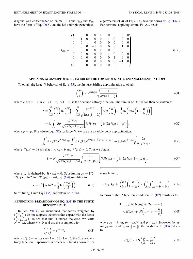
ENTANGLEMENT OF EXACT EXCITED STATES OF … PHYSICAL REVIEW B 98, 235156 (2018)
diagonal as a consequence of lemma F1. Thus Punit and Punit
have the forms of Eq. (D66), and the left and right generalizedeigenvectors of M of Eq. (F14) have the forms of Eq. (D67).Furthermore, applying lemma F1, Junit reads
Junit =
⎛⎜⎜⎜⎜⎜⎜⎜⎜⎜⎜⎜⎝
1 0 0 0 1 0 0 0 00 −1 0 0 0 1 0 0 00 0 1 0 0 0 0 0 00 0 0 −1 0 0 0 1 00 0 0 0 1 0 0 0 10 0 0 0 0 −1 0 0 00 0 0 0 0 0 1 0 00 0 0 0 0 0 0 −1 00 0 0 0 0 0 0 0 1
⎞⎟⎟⎟⎟⎟⎟⎟⎟⎟⎟⎟⎠. (F38)
APPENDIX G: ASYMPTOTIC BEHAVIOR OF THE TOWER OF STATES ENTANGLEMENT ENTROPY
To obtain the large-N behavior of Eq. (135), we first use Stirling approximation to obtain(N
α
)∼ eNH ( α
N)
√1
2πα(1 − α
N
) , (G1)
where H (x) ≡ −x ln x − (1 − x) ln(1 − x) is the Shannon entropy function. The sum in Eq. (135) can then be written as
I ≡N∑
α=0
(N
α
)ln
(N
α
)∼
N∑α=0
eNH ( αN
)√2πα
(1 − α
N
)[NH
(α
N
)− 1
2ln
(2πα
(1 − α
N
))]
≈ N
∫ 1
0dp
eNH (p)
√2πNp(1 − p)
[NH (p) − 1
2ln(2πNp(1 − p))
], (G2)
where p = αN
. To evaluate Eq. (G2) for large N , we can use a saddle point approximation:∫ b
a
dx g(x)eNf (x) ≈∫ b
a
dx g(x)eNf (x0 )+ N2 f ′′(x0 )(x−x0 )2 = g(x0)eNf (x0 )
√2π
N |f ′′(x0)| , (G3)
where f ′(x0) = 0 such that a < x0 < b and f ′′(x0) < 0. Thus we obtain
I = NeNH (p0 )
√2πNp0(1 − p0)
√2π
N |H ′′(p0)|[NH (p0) − 1
2ln(2πNp0(1 − p0))
], (G4)
where p0 is defined by H ′(p0) = 0. Substituting p0 = 1/2,H (p0) = ln 2 and H ′′(p0) = −4, Eq. (G4) simplifies to
I = 2N
(N ln 2 − 1
2ln
(πN
2
))(G5)
Substituting I into Eq. (135), we obtain Eq. (136).
APPENDIX H: BREAKDOWN OF EQ. (132) IN THE FINITEDENSITY LIMIT
In Sec. VIII C, we mentioned that terms weighted by( n
a)( n
k−a) do not suppress the terms that appear with the factor
( n
a)( n
k−a−b). To see that this is indeed the case, we write
N = pn, where p > 0, and use the asymptotic form(n
pn
)∼ enH (p), (H1)
where H (x) ≡ −x ln x − (1 − x) ln(1 − x), the Shannon en-tropy function. Expansions in orders of n breaks down if, for
some finite b,
∃ k1, k2 �(
n
k1
)(n
k − k1
)<
(n
k2
)(n
k − b − k2
). (H2)
In terms of the H function, condition Eq. (H2) translates to
∃ p1, p2 � H (p1) + H (p − p1)
< H (p2) + H
(p − p2 − b
n
), (H3)
where p1 ≡ k1/n, p2 ≡ k2/n, and p ≡ k/n. However, by us-ing p1 → 0 and p2 → p
2 − b2n
, the condition Eq. (H3) reducesto
H (p) < 2H
(p
2− b
2n
). (H4)
235156-39
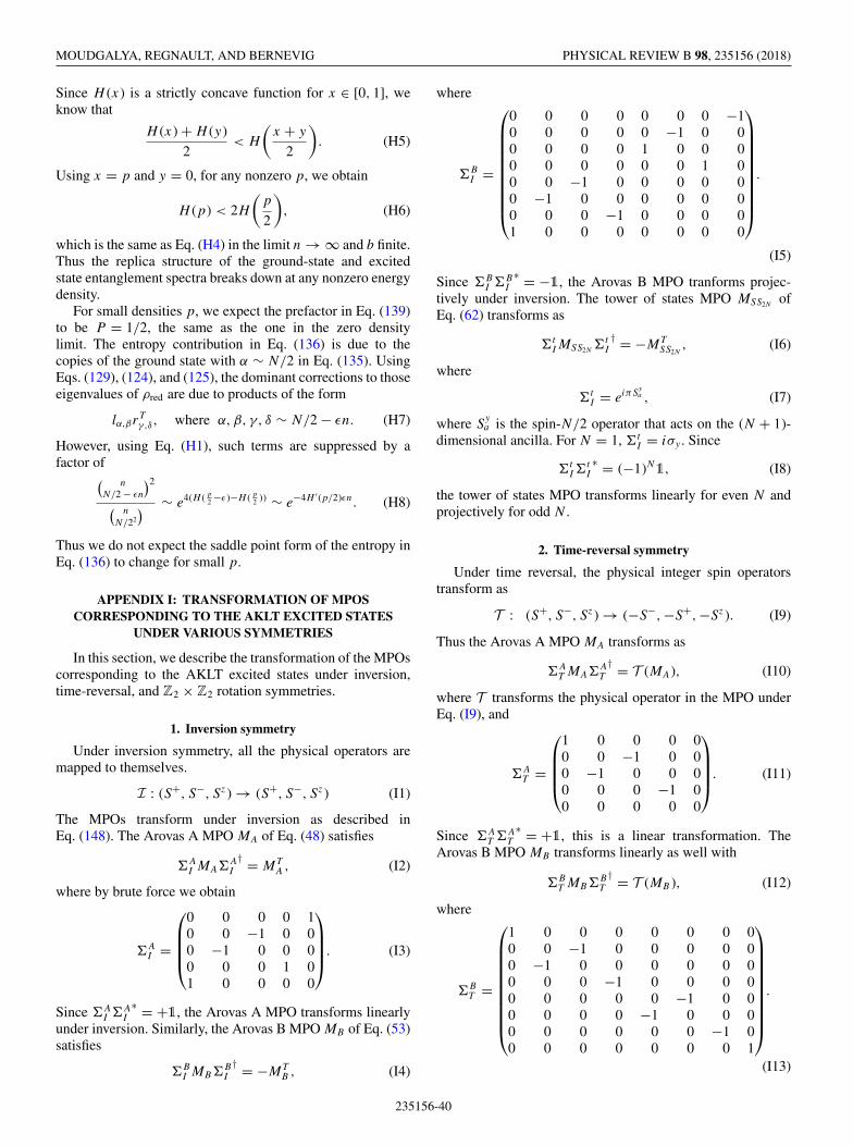
MOUDGALYA, REGNAULT, AND BERNEVIG PHYSICAL REVIEW B 98, 235156 (2018)
Since H (x) is a strictly concave function for x ∈ [0, 1], weknow that
H (x) + H (y)
2< H
(x + y
2
). (H5)
Using x = p and y = 0, for any nonzero p, we obtain
H (p) < 2H
(p
2
), (H6)
which is the same as Eq. (H4) in the limit n → ∞ and b finite.Thus the replica structure of the ground-state and excitedstate entanglement spectra breaks down at any nonzero energydensity.
For small densities p, we expect the prefactor in Eq. (139)to be P = 1/2, the same as the one in the zero densitylimit. The entropy contribution in Eq. (136) is due to thecopies of the ground state with α ∼ N/2 in Eq. (135). UsingEqs. (129), (124), and (125), the dominant corrections to thoseeigenvalues of ρred are due to products of the form
lα,βrTγ,δ, where α, β, γ, δ ∼ N/2 − εn. (H7)
However, using Eq. (H1), such terms are suppressed by afactor of(
n
N/2 − εn
)2( n
N/22
) ∼ e4(H ( p
2 −ε)−H ( p
2 )) ∼ e−4H ′(p/2)εn. (H8)
Thus we do not expect the saddle point form of the entropy inEq. (136) to change for small p.
APPENDIX I: TRANSFORMATION OF MPOSCORRESPONDING TO THE AKLT EXCITED STATES
UNDER VARIOUS SYMMETRIES
In this section, we describe the transformation of the MPOscorresponding to the AKLT excited states under inversion,time-reversal, and Z2 × Z2 rotation symmetries.
1. Inversion symmetry
Under inversion symmetry, all the physical operators aremapped to themselves.
I : (S+, S−, Sz) → (S+, S−, Sz) (I1)
The MPOs transform under inversion as described inEq. (148). The Arovas A MPO MA of Eq. (48) satisfies
�AI MA�A
I
† = MTA, (I2)
where by brute force we obtain
�AI =
⎛⎜⎜⎜⎝0 0 0 0 10 0 −1 0 00 −1 0 0 00 0 0 1 01 0 0 0 0
⎞⎟⎟⎟⎠. (I3)
Since �AI �A
I
∗ = +1, the Arovas A MPO transforms linearlyunder inversion. Similarly, the Arovas B MPO MB of Eq. (53)satisfies
�BI MB�B
I
† = −MTB , (I4)
where
�BI =
⎛⎜⎜⎜⎜⎜⎜⎜⎜⎜⎝
0 0 0 0 0 0 0 −10 0 0 0 0 −1 0 00 0 0 0 1 0 0 00 0 0 0 0 0 1 00 0 −1 0 0 0 0 00 −1 0 0 0 0 0 00 0 0 −1 0 0 0 01 0 0 0 0 0 0 0
⎞⎟⎟⎟⎟⎟⎟⎟⎟⎟⎠.
(I5)
Since �BI �B
I
∗ = −1, the Arovas B MPO tranforms projec-tively under inversion. The tower of states MPO MSS2N
ofEq. (62) transforms as
�tIMSS2N
�tI
† = −MTSS2N
, (I6)
where
�tI = eiπS
ya , (I7)
where Sya is the spin-N/2 operator that acts on the (N + 1)-
dimensional ancilla. For N = 1, �tI = iσy . Since
�tI�
tI
∗ = (−1)N1, (I8)
the tower of states MPO transforms linearly for even N andprojectively for odd N .
2. Time-reversal symmetry
Under time reversal, the physical integer spin operatorstransform as
T : (S+, S−, Sz) → (−S−,−S+,−Sz). (I9)
Thus the Arovas A MPO MA transforms as
�AT MA�A
T
† = T (MA), (I10)
where T transforms the physical operator in the MPO underEq. (I9), and
�AT =
⎛⎜⎜⎜⎝1 0 0 0 00 0 −1 0 00 −1 0 0 00 0 0 −1 00 0 0 0 0
⎞⎟⎟⎟⎠. (I11)
Since �AT �A
T
∗ = +1, this is a linear transformation. TheArovas B MPO MB transforms linearly as well with
�BT MB�B
T
† = T (MB ), (I12)
where
�BT =
⎛⎜⎜⎜⎜⎜⎜⎜⎜⎜⎝
1 0 0 0 0 0 0 00 0 −1 0 0 0 0 00 −1 0 0 0 0 0 00 0 0 −1 0 0 0 00 0 0 0 0 −1 0 00 0 0 0 −1 0 0 00 0 0 0 0 0 −1 00 0 0 0 0 0 0 1
⎞⎟⎟⎟⎟⎟⎟⎟⎟⎟⎠.
(I13)
235156-40
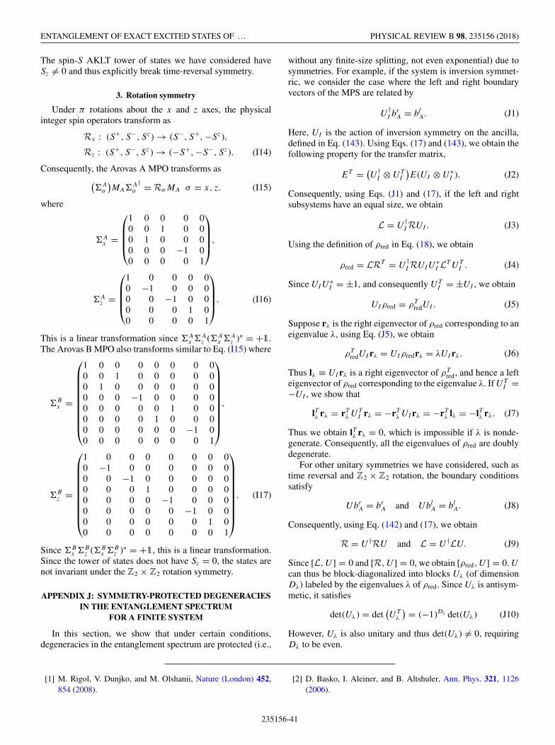
ENTANGLEMENT OF EXACT EXCITED STATES OF … PHYSICAL REVIEW B 98, 235156 (2018)
The spin-S AKLT tower of states we have considered haveSz �= 0 and thus explicitly break time-reversal symmetry.
3. Rotation symmetry
Under π rotations about the x and z axes, the physicalinteger spin operators transform as
Rx : (S+, S−, Sz) → (S−, S+,−Sz),
Rz : (S+, S−, Sz) → (−S+,−S−, Sz). (I14)
Consequently, the Arovas A MPO transforms as(�A
σ
)MA�A
σ
† = RσMA σ = x, z. (I15)
where
�Ax =
⎛⎜⎜⎜⎝1 0 0 0 00 0 1 0 00 1 0 0 00 0 0 −1 00 0 0 0 1
⎞⎟⎟⎟⎠,
�Az =
⎛⎜⎜⎜⎝1 0 0 0 00 −1 0 0 00 0 −1 0 00 0 0 1 00 0 0 0 1
⎞⎟⎟⎟⎠. (I16)
This is a linear transformation since �Ax �A
z (�Ax �A
z )∗ = +1.The Arovas B MPO also transforms similar to Eq. (I15) where
�Bx =
⎛⎜⎜⎜⎜⎜⎜⎜⎜⎜⎝
1 0 0 0 0 0 0 00 0 1 0 0 0 0 00 1 0 0 0 0 0 00 0 0 −1 0 0 0 00 0 0 0 0 1 0 00 0 0 0 1 0 0 00 0 0 0 0 0 −1 00 0 0 0 0 0 0 1
⎞⎟⎟⎟⎟⎟⎟⎟⎟⎟⎠,
�Bz =
⎛⎜⎜⎜⎜⎜⎜⎜⎜⎜⎝
1 0 0 0 0 0 0 00 −1 0 0 0 0 0 00 0 −1 0 0 0 0 00 0 0 1 0 0 0 00 0 0 0 −1 0 0 00 0 0 0 0 −1 0 00 0 0 0 0 0 1 00 0 0 0 0 0 0 1
⎞⎟⎟⎟⎟⎟⎟⎟⎟⎟⎠. (I17)
Since �Bx �B
z (�Bx �B
z )∗ = +1, this is a linear transformation.Since the tower of states does not have Sz = 0, the states arenot invariant under the Z2 × Z2 rotation symmetry.
APPENDIX J: SYMMETRY-PROTECTED DEGENERACIESIN THE ENTANGLEMENT SPECTRUM
FOR A FINITE SYSTEM
In this section, we show that under certain conditions,degeneracies in the entanglement spectrum are protected (i.e.,
without any finite-size splitting, not even exponential) due tosymmetries. For example, if the system is inversion symmet-ric, we consider the case where the left and right boundaryvectors of the MPS are related by
U†I b
rA = bl
A. (J1)
Here, UI is the action of inversion symmetry on the ancilla,defined in Eq. (143). Using Eqs. (17) and (143), we obtain thefollowing property for the transfer matrix,
ET = (U
†I ⊗ UT
I
)E(UI ⊗ U ∗
I ). (J2)
Consequently, using Eqs. (J1) and (17), if the left and rightsubsystems have an equal size, we obtain
L = U†IRUI . (J3)
Using the definition of ρred in Eq. (18), we obtain
ρred = LRT = U†IRUIU
∗I LT UT
I . (J4)
Since UIU∗I = ±1, and consequently UT
I = ±UI , we obtain
UIρred = ρTredUI . (J5)
Suppose rλ is the right eigenvector of ρred corresponding to aneigenvalue λ, using Eq. (J5), we obtain
ρTredUI rλ = UIρredrλ = λUI rλ. (J6)
Thus lλ ≡ UI rλ is a right eigenvector of ρTred, and hence a left
eigenvector of ρred corresponding to the eigenvalue λ. If UTI =
−UI , we show that
lTλ rλ = rTλ UT
I rλ = −rTλ UI rλ = −rT
λ lλ = −lTλ rλ. (J7)
Thus we obtain lTλ rλ = 0, which is impossible if λ is nonde-generate. Consequently, all the eigenvalues of ρred are doublydegenerate.
For other unitary symmetries we have considered, such astime reversal and Z2 × Z2 rotation, the boundary conditionssatisfy
UbrA = br
A and UblA = bl
A. (J8)
Consequently, using Eq. (142) and (17), we obtain
R = U †RU and L = U †LU. (J9)
Since [L, U ] = 0 and [R, U ] = 0, we obtain [ρred, U ] = 0. Ucan thus be block-diagonalized into blocks Uλ (of dimensionDλ) labeled by the eigenvalues λ of ρred. Since Uλ is antisym-metic, it satisfies
det(Uλ) = det(UT
λ
) = (−1)Dλ det(Uλ) (J10)
However, Uλ is also unitary and thus det(Uλ) �= 0, requiringDλ to be even.
[1] M. Rigol, V. Dunjko, and M. Olshanii, Nature (London) 452,854 (2008).
[2] D. Basko, I. Aleiner, and B. Altshuler, Ann. Phys. 321, 1126(2006).
235156-41

MOUDGALYA, REGNAULT, AND BERNEVIG PHYSICAL REVIEW B 98, 235156 (2018)
[3] R. Nandkishore and D. A. Huse, Annu. Rev. Condens. MatterPhys. 6, 15 (2015).
[4] V. Khemani, D. N. Sheng, and D. A. Huse, Phys. Rev. Lett. 119,075702 (2017).
[5] A. Pal and D. A. Huse, Phys. Rev. B 82, 174411 (2010).[6] J. A. Kjäll, J. H. Bardarson, and F. Pollmann, Phys. Rev. Lett.
113, 107204 (2014).[7] M. Žnidaric, T. Prosen, and P. Prelovšek, Phys. Rev. B 77,
064426 (2008).[8] D. J. Luitz, N. Laflorencie, and F. Alet, Phys. Rev. B 91, 081103
(2015).[9] J. H. Bardarson, F. Pollmann, and J. E. Moore, Phys. Rev. Lett.
109, 017202 (2012).[10] S. Iyer, V. Oganesyan, G. Refael, and D. A. Huse, Phys. Rev. B
87, 134202 (2013).[11] M. Rigol, Phys. Rev. Lett. 103, 100403 (2009).[12] S. D. Geraedts, N. Regnault, and R. M. Nandkishore, New J.
Phys. 19, 113021 (2017).[13] A. Chandran, V. Khemani, C. R. Laumann, and S. L. Sondhi,
Phys. Rev. B 89, 144201 (2014).[14] P. Fendley, J. Phys. A: Math. Theor. 49, 30LT01 (2016).[15] J. M. Deutsch, Phys. Rev. A 43, 2046 (1991).[16] M. Srednicki, Phys. Rev. E 50, 888 (1994).[17] D. A. Huse, R. Nandkishore, V. Oganesyan, A. Pal, and S. L.
Sondhi, Phys. Rev. B 88, 014206 (2013).[18] Y. Huang, Nucl. Phys. B 938, 594 (2019).[19] T.-C. Lu and T. Grover, arXiv:1709.08784.[20] Y. Huang and Y. Gu, arXiv:1709.09160.[21] C. Liu, X. Chen, and L. Balents, Phys. Rev. B 97, 245126
(2018).[22] J. Haegeman, S. Michalakis, B. Nachtergaele, T. J. Osborne, N.
Schuch, and F. Verstraete, Phys. Rev. Lett. 111, 080401 (2013).[23] I. Pizorn, arXiv:1202.3336.[24] J. Haegeman, B. Pirvu, D. J. Weir, J. I. Cirac, T. J. Osborne,
H. Verschelde, and F. Verstraete, Phys. Rev. B 85, 100408(2012).
[25] J. Haegeman, T. J. Osborne, and F. Verstraete, Phys. Rev. B 88,075133 (2013).
[26] J. Haegeman and F. Verstraete, Annu. Rev. Condens. MatterPhys. 8, 355 (2017).
[27] V. Zauner, D. Draxler, L. Vanderstraeten, M. Degroote, J.Haegeman, M. M. Rams, V. Stojevic, N. Schuch, and F.Verstraete, New J. Phys. 17, 053002 (2015).
[28] V. Zauner-Stauber, L. Vanderstraeten, J. Haegeman, I. P.McCulloch, and F. Verstraete, Phys. Rev. B 97, 235155 (2018).
[29] R. Thomale, S. Rachel, B. A. Bernevig, and D. P. Arovas,J. Stat. Mech.: Theor. Exp. (2015) P07017.
[30] U. Schollwöck, Ann. Phys. 326, 96 (2011).[31] R. Orús, Ann. Phys. 349, 117 (2014).[32] F. Verstraete and J. I. Cirac, Phys. Rev. B 73, 094423 (2006).[33] M. Friesdorf, A. H. Werner, W. Brown, V. B. Scholz, and
J. Eisert, Phys. Rev. Lett. 114, 170505 (2015).[34] V. Khemani, F. Pollmann, and S. L. Sondhi, Phys. Rev. Lett.
116, 247204 (2016).[35] X. Yu, D. Pekker, and B. K. Clark, Phys. Rev. Lett. 118, 017201
(2017).[36] N. Shiraishi and T. Mori, Phys. Rev. Lett. 119, 030601
(2017).[37] R. Mondaini, K. Mallayya, L. F. Santos, and M. Rigol, Phys.
Rev. Lett. 121, 038901 (2018).
[38] N. Shiraishi and T. Mori, Phys. Rev. Lett. 121, 038902 (2018).[39] C. Turner, A. Michailidis, D. Abanin, M. Serbyn, and Z. Papic,
Nat. Phys. (2018).[40] M. Schecter and T. Iadecola, Phys. Rev. B 98, 035139 (2018).[41] O. Vafek, N. Regnault, and B. A. Bernevig, SciPost Phys. 3, 043
(2017).[42] S. Moudgalya, S. Rachel, B. A. Bernevig, and N. Regnault,
Phys. Rev. B 98, 235155 (2018).[43] H. Fan, V. Korepin, and V. Roychowdhury, Phys. Rev. Lett. 93,
227203 (2004).[44] V. E. Korepin and Y. Xu, Int. J. Mod. Phys. B 24, 1361 (2010).[45] H. Katsura, T. Hirano, and Y. Hatsugai, Phys. Rev. B 76, 012401
(2007).[46] R. A. Santos, V. Korepin, and S. Bose, Phys. Rev. A 84, 062307
(2011).[47] R. A. Santos and V. E. Korepin, J. Phys. A: Math. Theor. 45,
125307 (2012).[48] R. A. Santos, F. N. Paraan, V. E. Korepin, and A. Klümper,
Europhys. Lett. 98, 37005 (2012).[49] R. A. Santos, F. N. Paraan, V. E. Korepin, and A. Klümper,
J. Phys. A: Math. Theor. 45, 175303 (2012).[50] R. A. Santos and V. Korepin, Quant. Info. Proc. 15, 4581
(2016).[51] H. Katsura, T. Hirano, and V. E. Korepin, J. Phys. Al 41, 135304
(2008).[52] Y. Xu, H. Katsura, T. Hirano, and V. E. Korepin, Quant. Info.
Proc. 7, 153 (2008).[53] Y. Xu, H. Katsura, T. Hirano, and V. E. Korepin, J. Stat. Phys.
133, 347 (2008).[54] H. Kim, T. N. Ikeda, and D. A. Huse, Phys. Rev. E 90, 052105
(2014).[55] J. R. Garrison and T. Grover, Phys. Rev. X 8, 021026 (2018).[56] F. Verstraete, V. Murg, and J. I. Cirac, Adv. Phys. 57, 143
(2008).[57] D. Perez-Garcia, F. Verstraete, M. M. Wolf, and J. I. Cirac,
Quant. Inf. Comput. 7, 401 (2007).[58] J. I. Cirac, D. Poilblanc, N. Schuch, and F. Verstraete,
Phys. Rev. B 83, 245134 (2011).[59] I. Affleck, T. Kennedy, E. H. Lieb, and H. Tasaki, Phys. Rev.
Lett. 59, 799 (1987).[60] A. Klümper, A. Schadschneider, and J. Zittartz, Europhys. Lett.
24, 293 (1993).[61] B. Pirvu, V. Murg, J. I. Cirac, and F. Verstraete, New J. Phys.
12, 025012 (2010).[62] I. P. McCulloch, J. Stat. Mech.: Theor. Exp. (2007) P10014.[63] F. Verstraete, J. J. Garcia-Ripoll, and J. I. Cirac, Phys. Rev. Lett.
93, 207204 (2004).[64] G. M. Crosswhite and D. Bacon, Phys. Rev. A 78, 012356
(2008).[65] J. Motruk, M. P. Zaletel, R. S. K. Mong, and F. Pollmann,
Phys. Rev. B 93, 155139 (2016).[66] D. P. Arovas, Phys. Lett. A 137, 431 (1989).[67] L. Vanderstraeten, M. Mariën, F. Verstraete, and J. Haegeman,
Phys. Rev. B 92, 201111 (2015).[68] B. Pirvu, J. Haegeman, and F. Verstraete, Phys. Rev. B 85,
035130 (2012).[69] D. P. Arovas, A. Auerbach, and F. D. M. Haldane, Phys. Rev.
Lett. 60, 531 (1988).[70] S. Yi, Ö. E. Müstecaplıoglu, C.-P. Sun, and L. You, Phys. Rev.
A 66, 011601 (2002).
235156-42

ENTANGLEMENT OF EXACT EXCITED STATES OF … PHYSICAL REVIEW B 98, 235156 (2018)
[71] D. P. Arovas, Phys. Rev. B 77, 104404 (2008).[72] S. M. Girvin, A. H. MacDonald, and P. M. Platzman, Phys. Rev.
B 33, 2481 (1986).[73] L. D’Alessio, Y. Kafri, A. Polkovnikov, and M. Rigol,
Adv. Phys. 65, 239 (2016).[74] C. Turner, A. Michailidis, D. Abanin, M. Serbyn, and Z. Papic,
Phys. Rev. B 98, 155134 (2018).[75] H. Bernien, S. Schwartz, A. Keesling, H. Levine, A. Omran, H.
Pichler, S. Choi, A. S. Zibrov, M. Endres, M. Greiner et al.,Nature (London) 551, 579 (2017).
[76] F. Pollmann, A. M. Turner, E. Berg, and M. Oshikawa,Phys. Rev. B 81, 064439 (2010).
[77] F. Pollmann, E. Berg, A. M. Turner, and M. Oshikawa,Phys. Rev. B 85, 075125 (2012).
[78] F. Pollmann and A. M. Turner, Phys. Rev. B 86, 125441(2012).
[79] X. Chen, Z.-C. Gu, and X.-G. Wen, Phys. Rev. B 83, 035107(2011).
[80] D. Pérez-García, M. M. Wolf, M. Sanz, F. Verstraete, and J. I.Cirac, Phys. Rev. Lett. 100, 167202 (2008).
[81] L. Vanderstraeten, F. Verstraete, and J. Haegeman, Phys. Rev. B92, 125136 (2015).
[82] D. Draxler, J. Haegeman, T. J. Osborne, V. Stojevic, L. Van-derstraeten, and F. Verstraete, Phys. Rev. Lett. 111, 020402(2013).
[83] S. Moudgalya, Y.-L. Wu, N. Regnault, and B. Bernevig(unpublished).
[84] J. Haegeman, M. Mariën, T. J. Osborne, and F. Verstraete,J. Math. Phys. 55, 021902 (2014).
[85] O. A. Castro-Alvaredo, C. De Fazio, B. Doyon, and I. M.Szécsényi, Phys. Rev. Lett. 121, 170602 (2018).
[86] O. A. Castro-Alvaredo, C. De Fazio, B. Doyon, and I. M.Szécsényi, J. High Energy Phys. 10 (2018) 39.
[87] V. Alba, M. Fagotti, and P. Calabrese, J. Stat. Mech.: Theor.Exp. (2009) P10020.
[88] J. Mölter, T. Barthel, U. Schollwöck, and V. Alba,J. Stat. Mech.: Theor. Exp. (2014) P10029.
[89] M. Sanz, M. M. Wolf, D. Perez-García, and J. I. Cirac,Phys. Rev. A 79, 042308 (2009).
[90] H.-H. Tu and M. Sanz, Phys. Rev. B 82, 104404 (2010).[91] M. Berry, Proc. R. Soc. London, Ser. A 423, 219 (1989).[92] K. Totsuka and M. Suzuki, J. Phys.: Condens. Matter 7, 1639
(1995).[93] M. Fannes, B. Nachtergaele, and R. Werner, Europhys. Lett. 10,
633 (1989).[94] M. Fannes, B. Nachtergaele, and R. F. Werner, Commun. Math.
Phys. 144, 443 (1992).[95] V. Karimipour and L. Memarzadeh, Phys. Rev. B 77, 094416
(2008).[96] A. K. Kolezhuk, H.-J. Mikeska, and S. Yamamoto, Phys. Rev.
B 55, R3336 (1997).[97] R. Fletcher and D. C. Sorensen, Am. Math. Mon. 90, 12 (1983).[98] P. Bartlett, Lecture 8: The Jordan Canonical Form, UCSB Math
108B, 2013.
235156-43


![arXiv:1709.04830v1 [cond-mat.mes-hall] 14 Sep 2017Following the proposal of Bernevig, Hughes, and Zhang [4], the QSH e ect was rst observed in HgTe/(Hg,Cd)Te quantum wells [5]; var-](https://img.pdfslide.us/doc/110x75/5e3ea1f796b2c742c0143f8b/arxiv170904830v1-cond-matmes-hall-14-sep-2017-following-the-proposal-of-bernevig.jpg)

![Bruce McKittrick Rare Books · 2019. 4. 24. · Catalogue Raisonné Du Cabinet. Paris, [Citoyenne Pitel for] F.L. Regnault-Delalande and J.C. Silvestre . vo. xiv, p. Slightly later](https://img.pdfslide.us/doc/110x75/6148bf3f2918e2056c22e388/bruce-mckittrick-rare-books-2019-4-24-catalogue-raisonn-du-cabinet-paris.jpg)


![arXiv:1104.1443v1 [astro-ph.CO] 7 Apr 2011 P. Ripoche · 2011-04-11 · in Regnault, Astier, Guy, et al. (2009, hereafter R09), and the simulations used to evaluate our survey selection](https://img.pdfslide.us/doc/110x75/5ec1525ff78c5c0dce69745e/arxiv11041443v1-astro-phco-7-apr-2011-p-ripoche-2011-04-11-in-regnault.jpg)