Physical Property Modeling

from Equations of State

David SchaichHope College REU 2003

Evaluation of Series Coefficients for the Peng-Robinson Equation

Summary of the Project

The goal of this project was to determine series coefficients for an analytic power series expansion of the Peng-Robinson equation of state.

This series can be used to give general expressions for accurate estimation of thermodynamical properties, as explicit functions of temperature, in the vapor-liquid coexistence region away from the critical point.

Results for terms up to 13th order in temperature were determined and tested for accuracy.

Only pure substances were considered in the course of this project.

Equations of State

RTVPnRTPV or

RT

VPTPZ ),(

• An equation of state is a functional relationship among the variables P, V, T

• Example: Ideal Gas Law

• Example: The Generalized Compressibility Factor (Z=1 for ideal gases)

Vapor-Liquid (Phase) Equilibrium

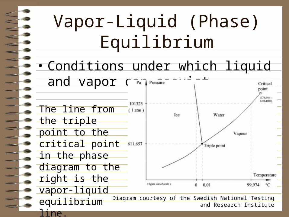
• Conditions under which liquid and vapor can coexist.

The line from the triple point to the critical point in the phase diagram to the right is the vapor-liquid equilibrium line.

Diagram courtesy of the Swedish National Testing and Research Institute

Using Equations of State

• All equations of state can predict one of the variables P, V, or T, given the other two.

• However, in order to predict phase equilibrium, one needs an equation of state capable of describing substances in both liquid and vapor phases.

• To do this, we can use cubic EoS, which take the form of cubic polynomials in molar volume.

A Few Notes Regarding Cubic EoS

• The three major cubic EoS have the same general form: a repulsive term derived from the ideal gas law, and an attractive term modeling van der Waals forces.

• All have a substance-specific constant b>0 that corrects for the volume occupied by the molecules themselves.

• All also have a term a>0 that influences the attractive van der Waals force. For more complex cubic EoS, a is a function of temperature and acentric factor.

• The Pitzer acentric factor (w) is a substance-specific constant that reflects the geometry and polarity of a molecule.

The Major Cubic EoS

2V

a

bV

RTP vdW

vdW

)(

),(

SRK

SRK

SRK bVV

TA

bV

RTP

22 2

),(

PRPR

PR

PR bbVV

TA

bV

RTP

termattractive termrepulsive

cSRKSRK T

TfaTA 1)(1),(

cPRPR T

TfaTA 1)(1),(

2176.574.1480.0)( f

2270.542.1375.0)( f

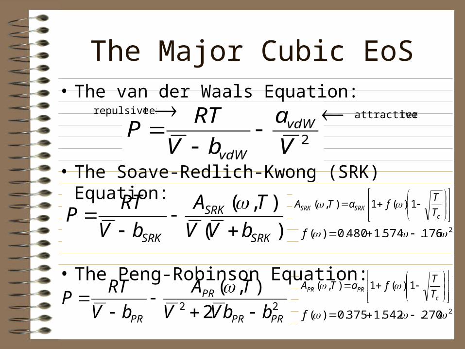
• The van der Waals Equation:

• The Soave-Redlich-Kwong (SRK) Equation:

• The Peng-Robinson Equation:

Pre

ssur

e

Volume

P > Vapor PressureOne real root -- Liquid

P < Vapor Pressure, One real root -- Vapor

P = Vapor Pressure Three real roots

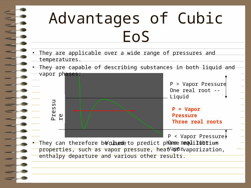
• They are applicable over a wide range of pressures and temperatures.

• They are capable of describing substances in both liquid and vapor phases:

• They can therefore be used to predict phase equilibrium properties, such as vapor pressure, heat of vaporization, enthalpy departure and various other results.

Advantages of Cubic EoS

Also...

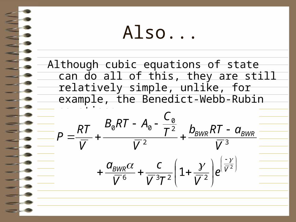
Although cubic equations of state can do all of this, they are still relatively simple, unlike, for example, the Benedict-Webb-Rubin equation:

2

2236

32

20

00

1 VBWR

BWRBWR

eVTV

c

V

a

V

aRTb

VTC

ARTB

V

RTP

The Series Approach

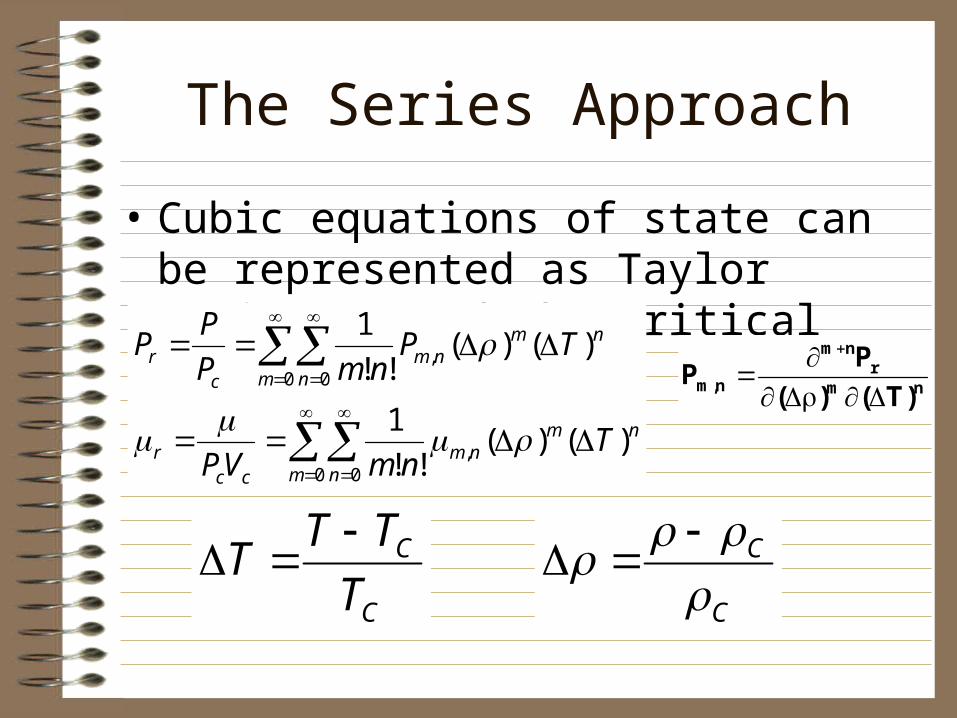
• Cubic equations of state can be represented as Taylor series around the critical point:

0 0,

0 0,

)()(!!

1

)()(!!

1

m n

nmnm

ccr

m n

nmnm

cr

TnmVP

TPnmP

PP

nm

rnm

n,m )T()(

PP

C

C

T

TTT

C

C

Simplifying the Series

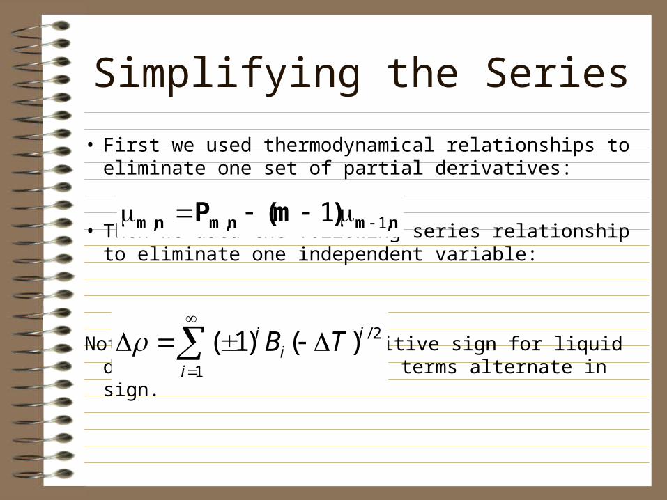
• First we used thermodynamical relationships to eliminate one set of partial derivatives:

• Then we used the following series relationship to eliminate one independent variable:

Note: All terms have a positive sign for liquid densities; for vapor, the terms alternate in sign.

n,mn,mn,m )m(P 11

1

2/)()1(i

ii

i TB

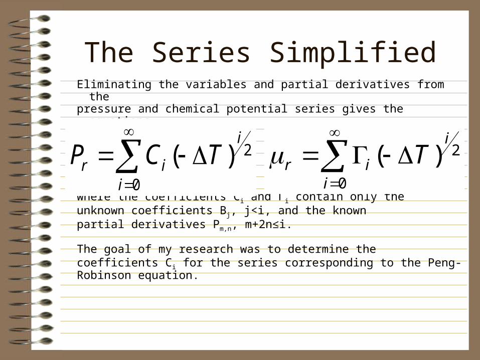
Eliminating the variables and partial derivatives from the pressure and chemical potential series gives the equations

where the coefficients Ci and Γi contain only theunknown coefficients Bj, j<i, and the known partial derivatives Pm,n, m+2n≤i.

The goal of my research was to determine the coefficients Ci for the series corresponding to the Peng-Robinson equation.

The Series Simplified

2

0

)(i

iir TCP

2

0

)(i

iir T

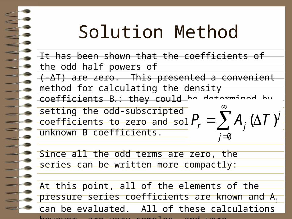
Solution MethodIt has been shown that the coefficients of the odd half powers of (-ΔT) are zero. This presented a convenient method for calculating the density coefficients Bi: they could be determined by setting the odd-subscripted C and Γ coefficients to zero and solving for the unknown B coefficients.

Since all the odd terms are zero, the series can be written more compactly:

At this point, all of the elements of the pressure series coefficients are known and Aj can be evaluated. All of these calculations however, are very complex, and were performed with programs written with the Maple mathematical software package.

j

jjr TAP )(

0

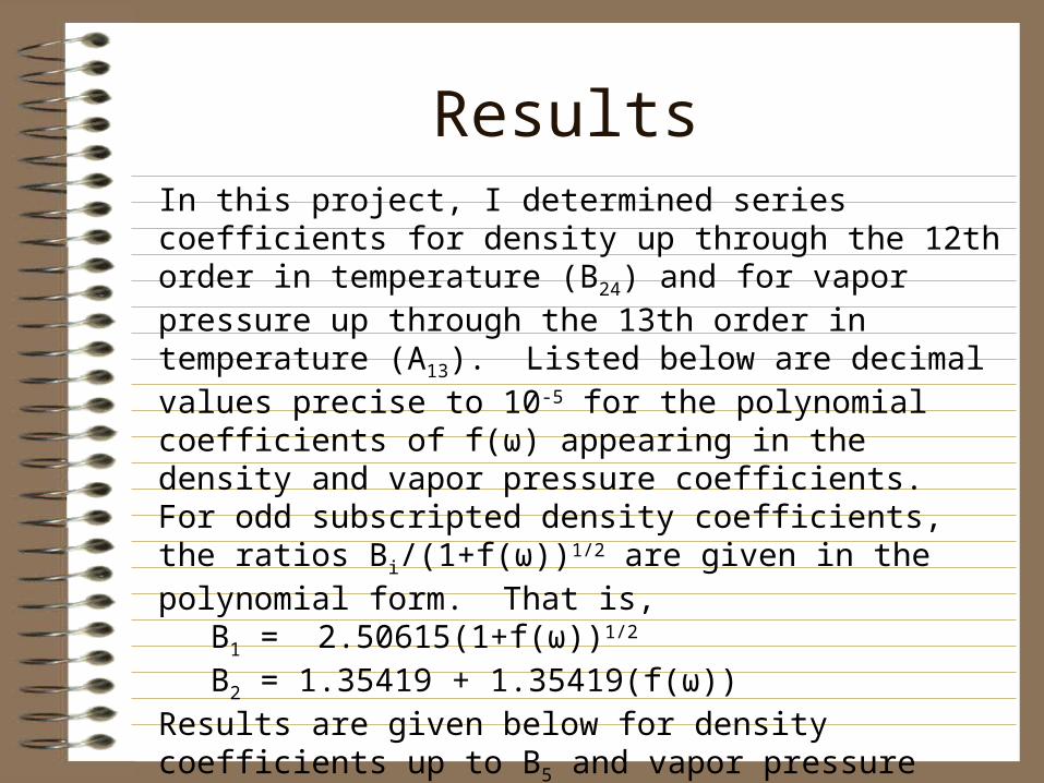
ResultsIn this project, I determined series coefficients for density up through the 12th order in temperature (B24) and for vapor pressure up through the 13th order in temperature (A13). Listed below are decimal values precise to 10-5 for the polynomial coefficients of f(ω) appearing in the density and vapor pressure coefficients. For odd subscripted density coefficients, the ratios Bi/(1+f(ω))1/2 are given in the polynomial form. That is,

B1 = 2.50615(1+f(ω))1/2 B2 = 1.35419 + 1.35419(f(ω))

Results are given below for density coefficients up to B5 and vapor pressure coefficients up to A5.

Complete results can be found at: http://www.amherst.edu/~daschaich/reu2003/results.htm

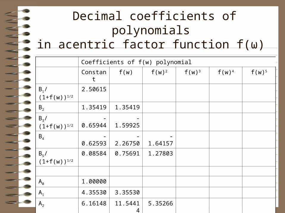
Decimal coefficients of polynomials in acentric factor function f(ω)

Coefficients of f(w) polynomial

Constant f(w) f(w)2 f(w)3 f(w)4 f(w)5

B1/(1+f(w))1/2 2.50615

B2 1.35419 1.35419

B3/(1+f(w))1/2 -0.65944 -1.59925

B4 -0.62593 -2.26750 -1.64157

B5/(1+f(w))1/2 0.08584 0.75691 1.27803

A0 1.00000

A1 4.35530 3.35530

A2 6.16148 11.54414 5.35266

A3 2.77903 11.85224 14.94798 5.87477

A4 0.42392 4.90733 14.63759 15.98672 5.83255

A5 1.00060 5.49346 15.06487 24.14467 19.88211 6.30944

Checking the ResultsWe checked our results by comparing the series' predictions for the vapor pressure of water over a range of temperatures with those of the equation itself (generated using an iterative solution method). If all coefficients in the series were correct, the difference between these two values would fit a curve one degree greater than that of the last term included in the series.

That is, if the series were truncated after the quadratic term in temperature, this difference should fit a cubic polynomial with respect to temperature deviation. If the series included terms up to the 13th power of temperature, the difference should be ≈14th power, as illustrated below.

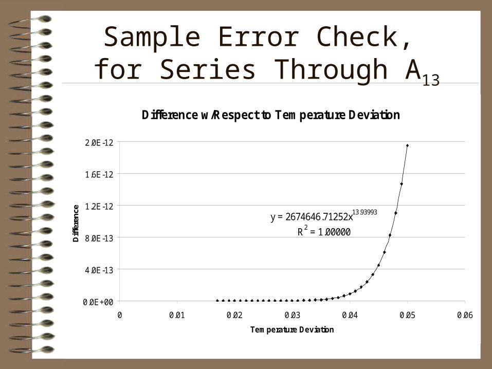
Difference w/Respect to Temperature Deviation

y = 2674646.71252x13.93993

R2 = 1.00000

0.0E+00

4.0E-13

8.0E-13

1.2E-12

1.6E-12

2.0E-12

0 0.01 0.02 0.03 0.04 0.05 0.06

Temperature Deviation

Diff

eren

ce

Sample Error Check, for Series Through A13

Future Plans

Currently, we are assessing the accuracy of the Peng-Robinson series over the whole range of temperatures and acentric factors. The chart below shows that the accuracy of the series decreases as temperature decreases and acentric factor increases.

In the future, the series can be used to generate predictions of equilibrium properties such as heat of vaporization and enthalpy departure.

At some point we will also attempt to move beyond pure solutions and adapt the series solutions for the Peng-Robinson and SRK equations to mixtures.

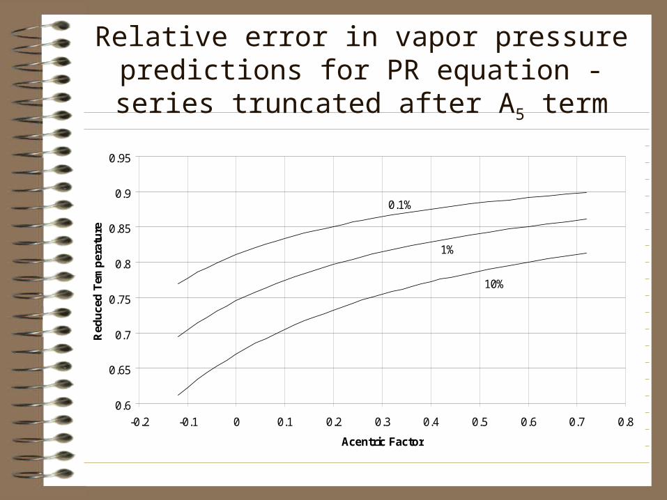
Relative error in vapor pressure predictions for PR equation - series truncated after A5 term

0.6

0.65

0.7

0.75

0.8

0.85

0.9

0.95

-0.2 -0.1 0 0.1 0.2 0.3 0.4 0.5 0.6 0.7 0.8

Acentric Factor

Red

uce

d T

emp

erat

ure

0.1%

1%

10%

Acknowledgments

I would like to thank:

– Dr. Misovich, for his expert guidance and assistance– The National Science Foundation, for its generous

funding– The Physics and Engineering Department at Hope

College– Scott Gangloff, John Alford and others who have

worked on this topic

Hope College