Embed Size (px)
Citation preview
503+
SAI/NW-81-250-04
PHYSICAL OCEANOGRAPHIC INVESTIGATIONS IN
THE BERING SEA MARGINAL ICE ZONE*
December 1981
by
Robin D. Muench
Science Applications, Inc.13400B Northrup Way, #36
Bellevue, Washington 98005
*This document is intended as a stand-alone attachment describing physicaloceanographic studies carried out in support of OCSEAP Research Unit #87,and comprises part of a draft final report to the University of Washingtonand to the OCSEAP program for this Research Unit.
TABLE OF CONTENTS
2.1.
2.2.
2.3.
2.4.
2.5.
INTRODUCTION . . . .
2.1.1., Summary. . .
2.1.2. Background .
2.1.3. Objectives .
FIELD PROGRAM. . . .
.
.
.
.
.
.
.
.
.
*..
.
.
.
.
.
.
.
.
.
.
..
.
..
.
.
.
.
.
.
.
.
.
.
..
.
.
.
.
.
..
.
.
..
.
.
..
.
..
.
.
.
.
..
.
..
.
..
.
.
.
..
.
.
.
.
2.2.1. Temperature and Salinity Observations.
2.2.2. Current Observations . . .. . . . . .. .
.
.
.
.
.
.
.
TEMPERATURE, SALINITY AND DENSITY DISTRIBUTIONS.
2.3.1.
2.3.2.
2.3.3.
CURRENT
November 1980. . . . . . . . . . . . . .
February-March 1981. . . . . . . . . . .
Temperature-Salinity Characteristics . .
OBSERVATIONS. . . . . . . . . . . . . .
DISCUSSION AND SUMMARY . . . . . . . . . . . . . .
2.5.1. Discussion. . . . . . . . . . . . . . .
2.5.2. Summary. . . . . . . . . . . . . . . . .
Acknowledgement. . . . . . . . . . . . . . . . . . . .
References. . . . . . . . . . . . . . . . . . . . . .
.
.
.
.
.
.
.
.
.
.
.
.
.
.
.
.
.
.
.
.
.
.
.
.
.
.
.
.
.
.
.
.
.
.
.
.
.
.
.
.
.
.
.
.
.
.
.
.
.
.
.
.
.
.
.
.
.
.
.
.
.
.
.
.
.
.
.
.
.
.
.
.
.
.
.
.
.
.
.
.
.
.
.
.
.
-.
.
.
.
.
.
.
.
.
.
.
.
.
.
.
.
.
.
.
.
.
.
.
.
.
.
.
.
.
.
.
.
.
.
.
.
.
.
.
.
.
.
.
.
.
.
.
.
.
.
.
.
.
.
.
.
.
.
.
.
.
.
.
.
.
.
.
.
.
.
.
.
.
.
.
.
.
.
.
.
.
Page
.
.
.
.
.
.
.
.
.
.
.
.
.
.
.
.
.
1
1
1
3
4
4
8
11
11
23
31
35
44
44
48
49
50
1
2.1. INTRODUCTION
2.1.1. S u m m a r y
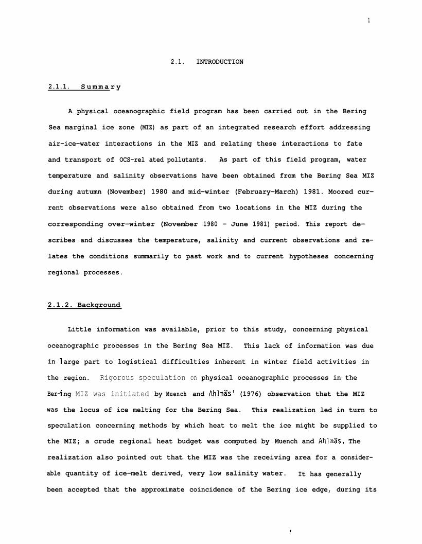
A physical oceanographic field program has been carried out in the Bering
Sea marginal ice zone (MIZ) as part of an integrated research effort addressing
air-ice-water interactions in the MIZ and relating these interactions to fate
and transport of OCS-rel ated pollutants. As part of this field program, water
temperature and salinity observations have been obtained from the Bering Sea MIZ
during autumn (November) 1980 and mid-winter (February-March) 1981. Moored cur-
rent observations were also obtained from two locations in the MIZ during the
corresponding over-winter (November 1980 - June 1981) period. This report de-
scribes and discusses the temperature, salinity and current observations and re-
lates the conditions summarily to past work and to current hypotheses concerning
regional processes.
2.1.2. Background
Little information was available, prior to this study, concerning physical
oceanographic processes in the Bering Sea MIZ. This lack of information was due
in -
the
Ber-
was
arge part to logistical difficulties inherent in winter field activities in
region. Rigorous speculation on physical oceanographic processes in the
ng MIZ was initiated by Muench and Ahln5s’ (1976) observation that the MIZ
the locus of ice melting for the Bering Sea. This realization led in turn to
speculation concerning methods by which heat to melt the ice might be supplied to
the MIZ; a crude regional heat budget was computed by Muench and Ahlnas. The
realization also pointed out that the MIZ was the receiving area for a consider-
able quantity of ice-melt derived, very low salinity water. It has generally
been accepted that the approximate coincidence of the Bering ice edge, during its
2
winter period of maximum southward extent, with the shelf break suggests an in-
teraction’ between ice edge-related and shelf break oceanographic processes. This
interaction has not been, however, rigorously explored.
Temperature-salinity data were obtained along the Bering Sea MIZ in mid-
winter 1979 and reported on by Pease (1980). She noted that the ice edge was
underlain by a two-layered water structure wherein a warmer, more saline lower
layer underlay a colder, lower salinity upper layer. Similar water structures
underlying the ice edge were noted using mid-late winter data from 1975 and 1976
(Niebauer et al., 1981). Finally, Newton and Andersen (1980) noted the same
structure associated with the Bering ice edge in winter 1980 temperature-salinity
data. These data, obtained prior to the present study, supported the concept of
a water structure two-layered in temperature and salinity underlying the ice
edge.
A theoretical argument for presence along the ice edge of wind-driven up-
welling similar in nature to coastal upwelling was advanced by Clarke (1978).
More recent work with numerical modeling techniques has suggested, however, that
the off-ice winds which would lead to upwelling also lead to breakup of a dis-
crete ice edge into bands, which in turn destroys the tendency toward upwelling
(L. P. Rfled, personal communication, 1981). At the present time, it therefore
appears unlikely that wind-induced upwelling at the ice edge is a significant
factor in the dynamics there. Hypotheses concerning the process have not yet,
however, been fully developed.
Development of additional speculations or hypotheses concerning Bering Sea
MIZ processes awaits further analysis of existing data or acquisition of new data.
This report, by providing a summary analysis of newly obtained data, will further
the development of knowledge on such processes.
2.1.3. Objectives
Overall objectives of the Bering Sea MIZ physical oceanographic program are
to derive information on oceanographic processes associated with the MIZ which
exert control over the fate and effects of OCS-related pollutants. Specific
program objectives include:
. Definition of the large-scale (i.e. of order hundreds of km) fields oftemperature and salinity (and derived density) and relating of these toregional oceanographic advective (transport) and diffusive (mixing) pro-cesses.
. Observation of small-scale (1-10 km) features (such as low salinity lensesand frontal structures) in the temperature and salinity distributionsalong the ice edge during winter and relating these where possible to re-gional oceanographic features, ice motion and distribution, and the windfield.
c Estimation, in conjunction with sea ice and meteorological data, of re-gional heat and salt balances.
. Estimation of the effects upon the water column of convective processesassociated with local winds and with ice freezing.
. Estimation of the effects of both large- and small-scale water circulationfeatures upon ice motion and distribution in the MIZ.
2.2. FIELD PROGRAM
2.2.1. Temperature and Salinity Observations
4
Two field activities involving temperature and salinity observations have
been carried out under this program: an autumn (November 1980) observation pro-
gram of regional temperature and salinity distributions combined with current
meter mooring deployments, and a mid-winter (February-March 1981) program of de-
tailed temperature and salinity observations along the ice edge. The mid-winter
program was carried out simultaneously with intensive observations of meteorolog-
ical and sea ice features. Recovery of the current meters which had been deployed
in November 1980 was carried out in June 1981.
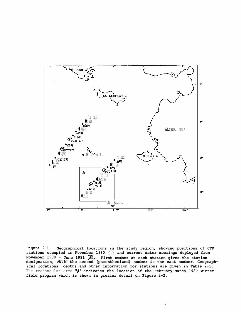
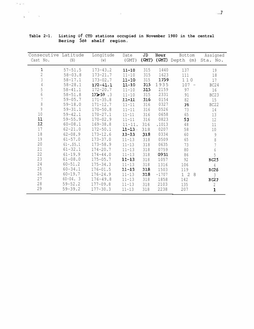
During the November 1980 program, 25 CTD casts were occupied in the portion
of the Bering Sea normally occupied by the MIZ during winter (Figure 2-1). These
CTD data were acquired from the
CTD system with calibration and
specifications. These November
NOAA vessel DISCOVERER using a Plessey Model 9040
processing procedures carried out as per OCSEAP
CTD data provide two transects extending across
the shelf normal to the isobaths from about the shelf break to the 50-meter iso-
bath and give a good representation of conditions over the central Bering Sea
shelf including the MIZ. The observed distributions are discussed in the follow-
ing section of this report. A listing of the autumn 1980 CTD stations is given
in Table 2-1.
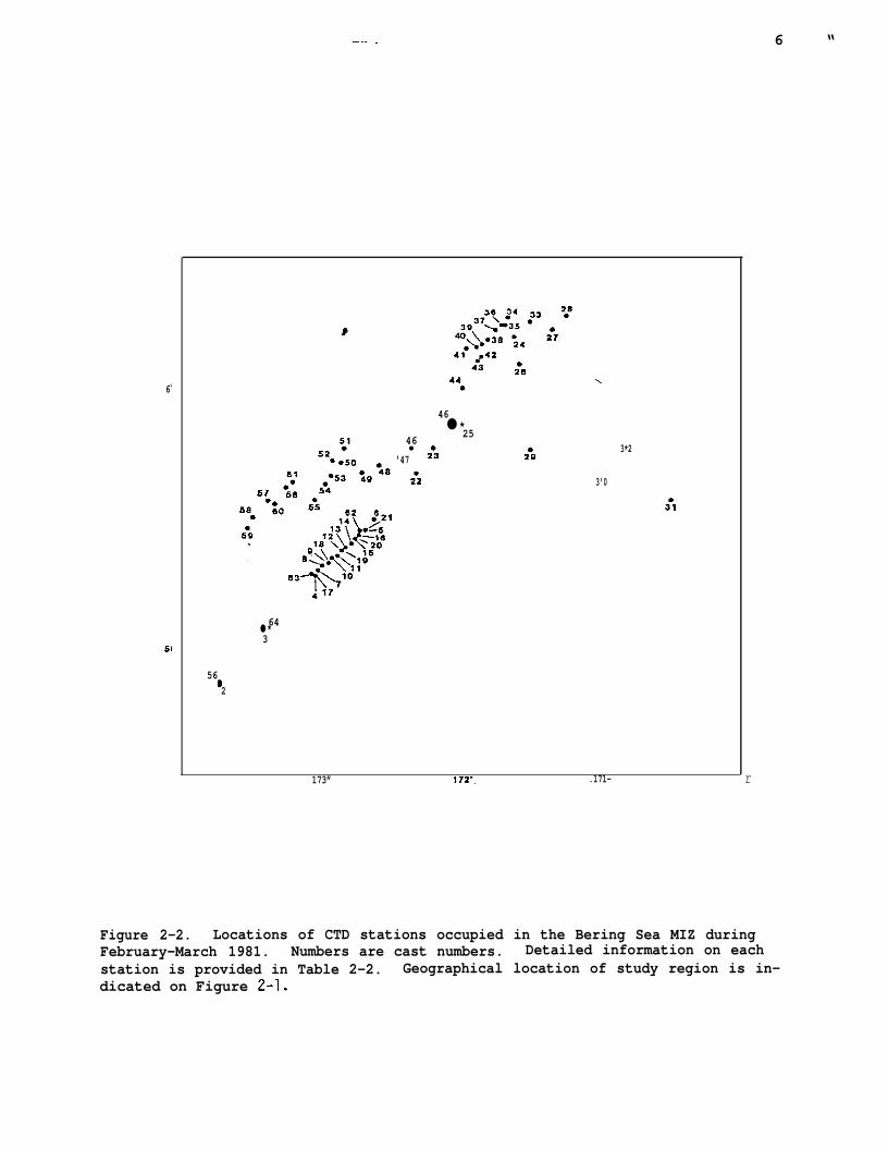
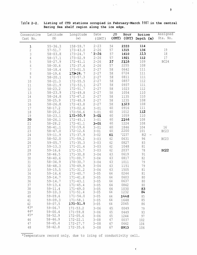
During the February-March 1981 field program, 64 CTD casts (2-65, Figure 2-2)
were taken in the Bering Sea MIZ near the ice edge. (The initial single cast (1)
was taken in the Gulf of Alaska near Unimak Pass for equipment calibration pur-
poses.) These CTD data were taken from the NOAA vessel SURVEYOR using a Plessey
Model 9040 CTD system; calibration casts were taken every third station. The
geographical location of the winter field work within the overall study region
910 (171● 9W3)
‘8(19)● 7(20]
(’
ALASKA (USA)‘6(21]
@Bg:,;3}%(24
@BC26125)● 3[26)
%C27[27)●2128)
‘1(29)
#
<.% Matthew I.‘111121
‘12(11)● 13[\o)
A q:;;:;)‘15(7 I
● BC23@)G&$,
● 17(3]‘18(2)
● 1911)
St. Paul Ld“? t 1 I , I ,
30 1 74Q i 7P 16.60 162°
Figure 2-1. Geographical locations in the study region, showing positions of CTDstations occupied in November 1980 (.) and current meter moorings deployed fromNovember 1980 - June 1981 (@). First number at each station gives the stationdesignation, while the second (parenthesized) number is the cast number. Geograph-ical locations, depths and other information for stations are given in Table 2-1.The rectangular area “A” indicates the location of the February-March 198? winterfield program which is shown in greater detail on Figure 2-2.
—.. .
6$
61
46●
‘47
2:
46● *
25
2°3
64● *3
5682
2’”
\
3*2
3’0
173” 172-. .171-
6 “
r
Figure 2-2. Locations of CTD stations occupied in the Bering Sea MIZ duringFebruary-March 1981. Numbers are cast numbers. Detailed information on eachstation is provided in Table 2-2. Geographical location of study region is in-dicated on Figure 2-1.
. . .
Table 2-1. Listing of CTD stations occupied in November 1980 in the centralBering Sea shelf region.
Consecutive Latitude Longitude Date Bottom AssignedCast No. (N) (w) (GMT) (&T) ?=T) Depth (m) Sta. No.
1 57-51.52 58-03.83 58-17.14 58-28.15 58-41.16 58-51.87 59-05.78 59-18.09 59-31.1
10 59-42.111 59-55.912 60-08.117 62-21.018 62-08.919 61-57.020 61-.$5.121 61-32.122 61-19.923 61-08.024 60-51.225 60-34.126 60-19.727 60–04. 328 59-52.229 59-39.2
173-43.2173-21.7173-02.7172–41.1172-20.717*59 .3171-35.8171-12.7170-50.8170-27.1170-02.9169-38.8172-50.1173-12.6173-37.0173-58.9174-20.7174-44.0175-05.7175-34.3176-01.5176-24.9176-49.8177-09.8177-30.3
11-10 31511-10 31511-10 31511–10 31511-10 31511-10 31511-11 31611-11 31611-11 31611-11 31611-11 31611-11. 31611-13 31811-13 31811-13 31811-13 31811-13 31811-13 31811-13 31811-13 31811-13 31811-13 31811-13 31811-13 31811-13 318
144016231759
19352159233101540327052606580823.1013020703340509063507590931105713161503-1707185821032238
137 19111 181 1 0 17107 - BC2497 1691 BC2382 1576 BC2273 1465 1353 1248 1158 1060 965 873 780 686 592 BC25
106 4119 BC.261 2 8 3142 B@7135 2207 1
8
is indicated on Figure 2-1; the winter CTD station work included occupation of “
the outer (southern) eight stations on the southeastern transect shown on .
Figure 2-1, mult”
taken along the
in Table 2-2.
ple occupation of a portion of this transect, and time series
ce edge. A listing of the winter 1981 CTD stations is given “
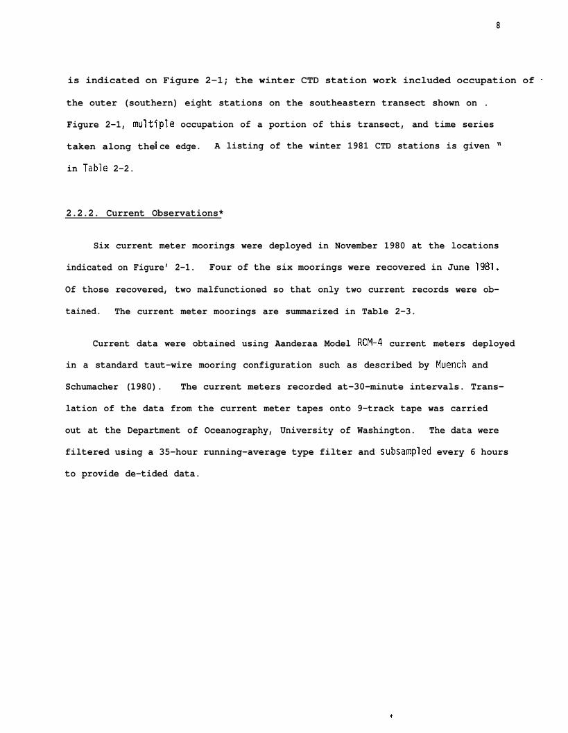
2.2.2. Current Observations*
Six current meter moorings were deployed in November 1980 at the locations
indicated on Figure’ 2-1. Four of the six moorings were recovered in June 1981.
Of those recovered, two malfunctioned so that only two current records were ob-
tained. The current meter moorings are summarized in Table 2-3.
Current data were obtained using Aanderaa Model RCM-4 current meters deployed
in a standard taut-wire mooring configuration such as described by Muench and
Schumacher (1980). The current meters recorded at-30-minute intervals. Trans-
lation of the data from the current meter tapes onto 9-track tape was carried
out at the Department of Oceanography, University of Washington. The data were
filtered using a 35-hour running-average type filter and subsampled every 6 hours
to provide de-tided data.
t
. . . .. .
9
Table 2-2. Listing of CTD stations occupied in February-March 1981 in the centralBering Sea shelf region along the ice edge.
Consecutive Latitude Longitude Date AssignedCast No. (N) (w) (GMT) (&T) !O=T) D~~=~O’?m) Sta. No.
123456789
10111213141516171819202122232425262728293031323334353637383940414243*44*45*464748
55-36.357-51.758-03.858-17.158-27.958-30.658-18.458-19.458-20.158-21.358-21.958-23.258-23.958–24.858-25.958-26.858-17.258-20.258-23.158-26.158-28.258-41.158–47.059-11.958-52.059-05.759-13.359-16.658-46.558-40.658-34.958-48.359-15.559-16.459-14.759-14.759-13.459-11.459-10.359-09.659-09.359-07.559-06.759-00.458-52.958-46.958-45.458-42.8
158-59.7173-43.0173-24.7173-02.9172-41.1172-37.6173-01.517%59. 7172-57.3172-55.5172-53.1172-51.7172-49.8172-47.2172-4$.9172-43.8173-02.6172-56.6172=50.9172-45.1172-41.1172-19.6172-12.6171-37.9171-59.2171-35.3171-21.4171-15.7171-30.8171-00.7170-30.7170-49.9171-31.2171-40.7171-41.8171-43.1171-45.4171-49.0171-51.4171-54.0171-58.1171-51.9171-53.2171-59.8172-05.6172-22.1172-27.7172-35.6
2-232-26
-2-262-262-262-262-272-272-272-272-272-272-272-272-272-273-013–013-013-013-013-013–013-023-033-033-033-033-043-043-043-043-043-053-053-053-053–053-053-053-053-053-063-063-063-083-083-08
545757575757585858585858585858586060606060606061626262626363636363646464646464646464656565676767
23331315161019212116225506420724081108570937102310541135123513230916101210591146122418462200‘2237063108271048203706190817101111511505024406030637084210301232144816482045004904491244003704420915
11413611311210910811111111111211111211011010810811111211010810810410182 -96838178918279798181808080
:2858586799397
102104106
191817
BC24
16BC23
BC23
BC22
*Temperature record only, due to icing of conductivity cell.
. .
10
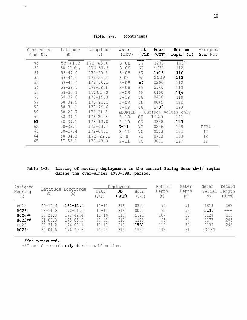
Table. 2-2. (continued)
Consecutive Latitude Longitude Date AssignedCast No. (N) (w) (GMT) (#T) YG~) “D~~i”?m) Sea. No.
“49 58-41.3 172-43.0— ---
3-08 67 1230 108--.50 58-43.6 , 172-51.8 3-08 67 ‘1654 11251 58-47.0 172-50.5 3-08 67 1913 11052 58-44.0 172-55.5 3-08 “67 2029 “11253 58-40.6 172-56.1 3-08 67 2200 11254 58-38.7 172-58.6 3-08 67 2340 11355 58-35.1 17303.0 3-09 68 0100 1~456 58-37.8 173-15.3 3-09 68 0438 11957 58-34.9 173-23.1 3-09 68 0845 12258 58-31.1 173-29.6 3-09 68 1232 12359 58-28.7 173-31.5 ABORTED - Surface values only60 58-34.1 173-20.3 3-10 69 1940 12161 58-39.1 173-12.8 3-10 69 2348 11962 58-28.1 172-43.7 3-11 70 0236 108 BC24 .63 58-17.4 173-04.1 3-11 70 0513 112 1764 58-04.3 173–22.2 3-n 70 0703 113 1865 57-52.1 173-43.3 3-11 70 0851 137 19
Table 2-3. Listing of mooring deployments in the central Bering Seas helf regionduring the over-winter 1980-1981 period.
Assigned Latitude LongitudeDeployment Bottom Meter Meter Record
Mooring (N) (w)Date Hour Depth Depth Serial Length
ID (GMT) (a) (GMT) (m) (m) No. (days)
BC22 59-10.4 171-11.4 11-11 316 0357 76 51 1813 207BC23* 58-51.8 172-01.0 11-11 316 0007 95 52 3130 ---BC24** 58-28.3 172-42.4 11-10 315 2021 107 59 3128 110BC25** 61-08.3 175-05.9 11-13 318 1128 95 52 3177 205BC26 60-34.2 176-02.1 11-13 318 1531 119 52 3135 203BC27* 60-04.6 176-49.6 11-13 318 1927 142 61 3131 ---
*Not recovered.**T and C records only due to malfunction.
11
2.3. TEMPERATURE, SALINITY AND DENSITY DISTRIBUTIONS
2:3.1. November 1980
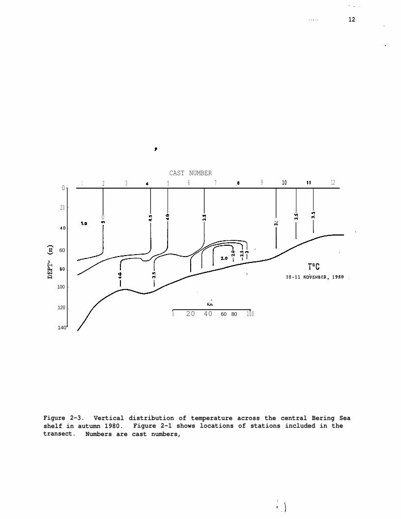
Vertical distributions of temperature, salinity and density along the two
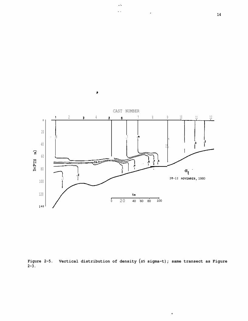
CTD transects occupied in November 1980 are shown in Figures 2-3 to 2-8. The~.
following features were common to both transects:
. The water~olumn was,two-layered vertically in temperature, salinity anddensity, with the interface between layers occurring at 50-60 m. Thewater was vertically well mixed above and below the interface. The in-terface between layers was 5-10 m shallower at the northwest than at thesoutheast transect, and was about 10-in thick.
. There was a relatively constant northeastward decrease in temperature,salinity and density in both the upper and lower layers in both transects.The ensuing horizontal gradients in either layer were approximately0.01 OC/km, 0.003 O/oo/km and 0.003 sigma-t units/km, respectively.
● There was a tendency for slightly increased horizontal temperature andsalinity gradients in both layers at the 80-90 m isobaths. However, thiswas not true for density due to the canceling effects exerted by the op-posing temperature and salinity gradients on the density gradient.
. At about the 80-m isobath, there was a 50-krn wide “bolus” of water whichwas about 1 ‘C colder than the surrounding water. This feature appearedon both transects, though the temperature of the bolus was about 2.5 ‘Clower on the northwest transect.
While the major feature
similarity in distributions,
of the comparison between the two transects was the
overall water temperatures at the northwest transect
were about 2 *C lower than to the southeast. Salinity and density were similar
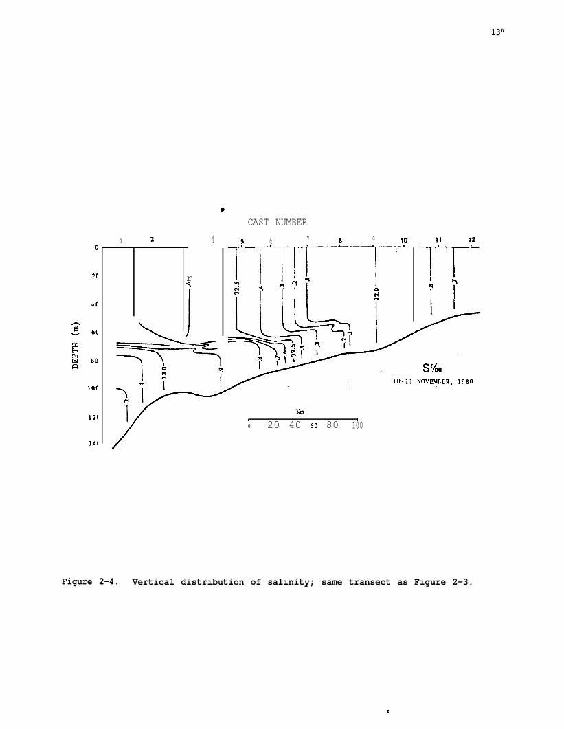
along the two transects. In the southeast section, there was some indication of
salinity finestructure at the interface between layers (stations 3, 4 and 8,
Figure 2-4); such finestructure was not evident anywhere in the transect to the
northwest.
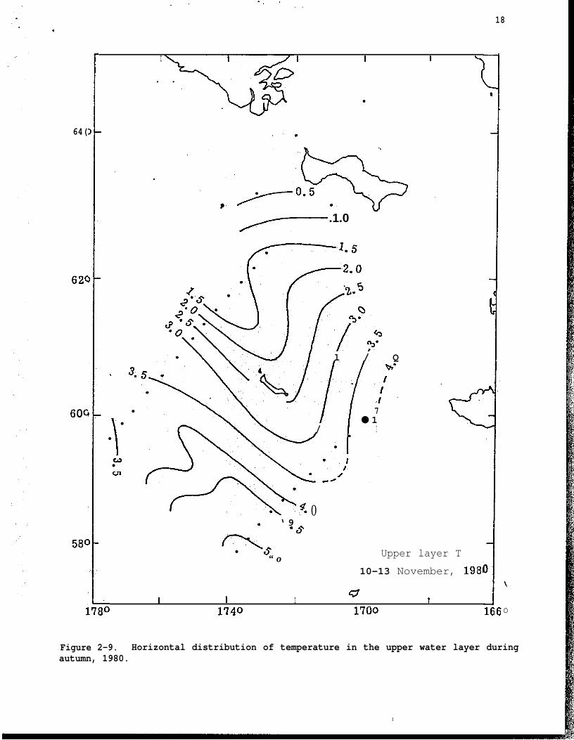
The tendency for water temperature to be lower along the northwest section
is evident in the horizontal distributions of temperature in the upper and lower
layers (Figures 2-9 and 2-10). The upper layer distribution shows maximum
. . .
—- . . . 12
0-
20 -
40 -
~ 60
xE go .~
100 -
120 .
140”
*
CAST NUMBER
1 2 3 4 5 6 7 ,8 9 10 11 12
0 m VI Ine + ~:A m.
/----’.
/
8Km
#o 20 40 60 80 100
Figure 2-3. Vertical distribution of temperature across the central Bering Seashelf in autumn 1980. Figure 2-1 shows locations of stations included in thetransect. Numbers are cast numbers,
13”
1 2 4
rq
J
CAST NUMBER
3 & 7 8 9 10
-N/ +--”.“
/
I KmI (o 20 40 60 80 100
Figure 2-4. Vertical distribution of salinity; same transect as Figure 2-3.
. ..
. . . 14
CAST NUMBER
o
20
40
s60
EP-1wa 80
100
120
140
,1.9
II 15.
XmI , r 1
0 20 40 60 80 100
11 121 2 3 4 7 6 7 8 9 10
.7 .e‘ ‘T
.3Ii
<
.3 10-11 NOVIW!ER, 1980
Figure 2-5. Vertical distribution of density (as sigma-t); same transect as Figure2-3.
t
.,
*.
20 -
40 -
60 -
80
100 -
120 -
140 -
lbO -
lBO”
2oo -
15 -—
CAST NUMBER
/:
hi ● .u Io(+
Xmo *
20 40 60 80 100
/’.
T * C13 NOV13111CR, 1980
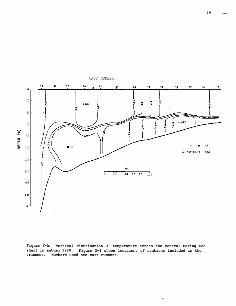
Figure 2-6; Vertical distribution of temperature across the central Bering Seashelf in autumn 1980. Figure 2-1 shows locations of stations included in thetransect. Numbers used are cast numbers.
..-.
CAST NUMBiR
40
60
Bo
100
120
140
160
1 B(
20[
\
2? - 21 27
0, w.
13 NOVIXBER, 1980
h—.2 - ~
o 20 40 100r.
!
b
I
I
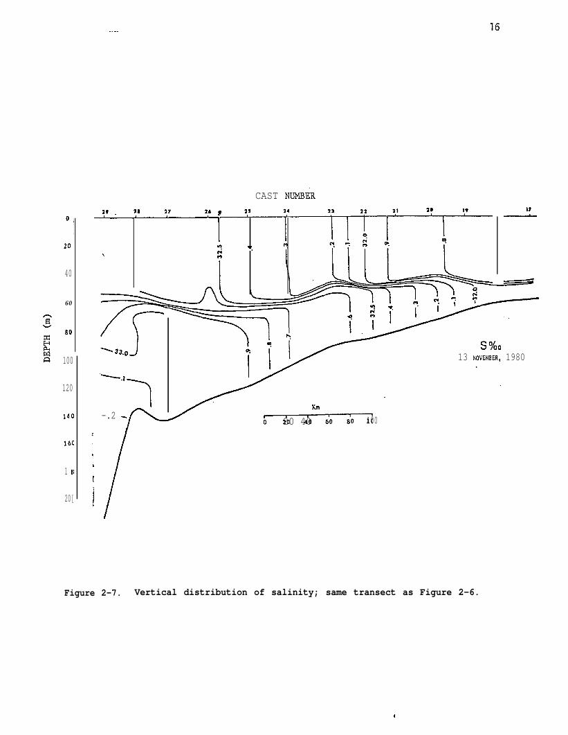
Figure 2-7. Vertical distribution of salinity; same transect as Figure 2-6.
—..
CAST NUMBER
o
20 -
40 -
60 -
80 “
100 “
120 “
.140-
160-
10o -
2oo -
2* 2B 27 26 2s 24 ?3
*m. m.
13 NOVEMBER, 19R0
/)Arn-
20 20 40 60 80 100
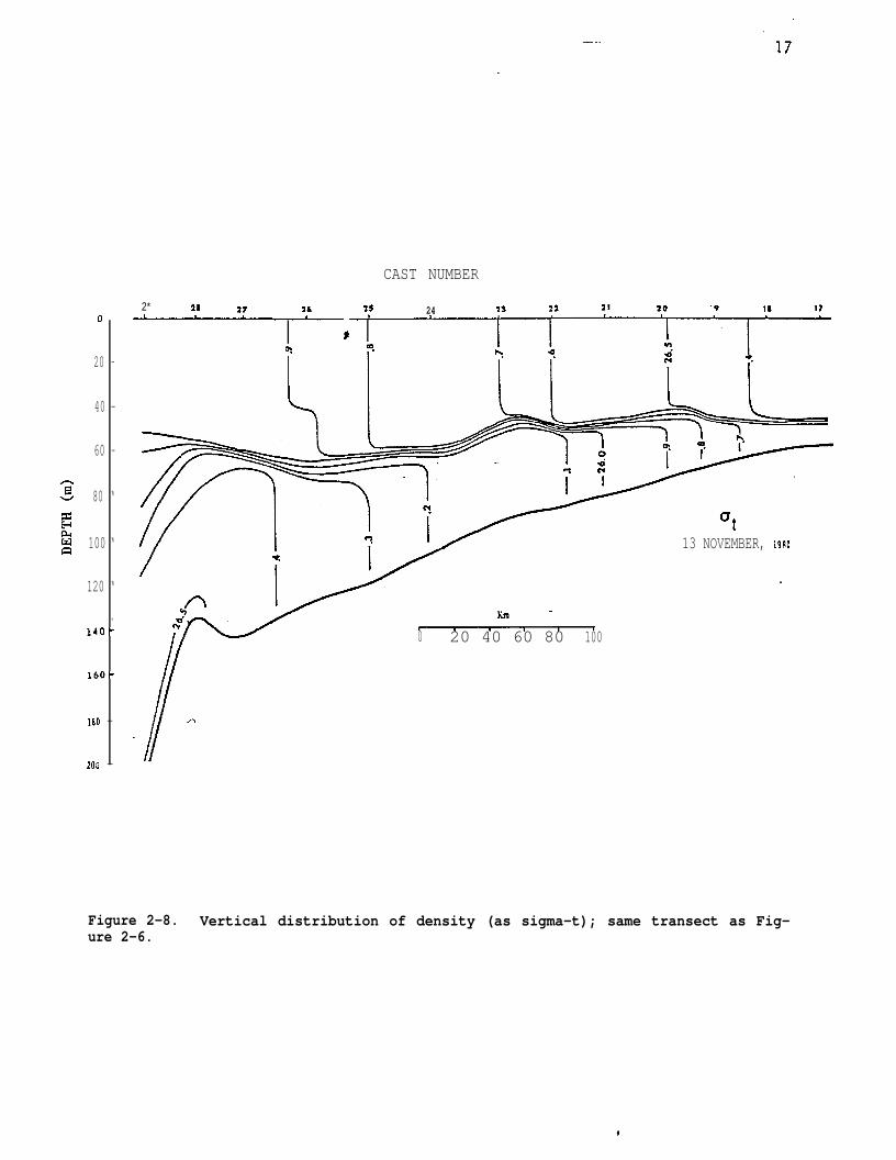
Figure 2-8. Vertical distribution of density (as sigma-t); same transect as Fig-ure 2-6.
,
64(
(j2C
60(2
58C
.’. -“.. .
18
I i I I \
. . (●
.
.
.
..-.
.1.0
.
\
●
●
u●
a
/------1;50.
3.
●
‘ 9
<“rs
● $“ o
l / Q
‘1 7● 1
/ I
0
Upper layer T
10-13 November, 198(o I1 I I o
17’80I
1740 1700
Figure 2-9. Horizontal distribution of temperature in the upper water layer duringautumn, 1980.
\
o
1
19-. —..
640
(52(
60’
58{~g”o+
. Lower la~er T
10-13 November. 198[
dI
I-
I 1 I I
1780 1740 1700 1660
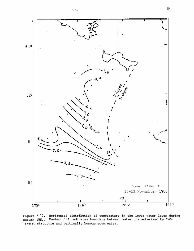
Figure 2-10. Horizontal distribution of temperature in the lower water layer duringautumn 1980. Dashed line indicates boundary between water characterized by two-Iayered structure and vertically homogeneous water.
.--20
temperatures
to less than
temperature
higher than 5 “C in the southern portion, with temperatures down
0.5 “C in the north. The distribution shows a “tongue’’-like, low-
< 3.5 ‘C) feature extending toward the southeast from the northwest,
with higher temperatures to the east along the Alaskan coast (4.0 ‘C) and to the
southwest toward the shelf break (3.5-5.0 ‘C).
Lower layer temperatures (Figure 2-10) showed a similar pattern, except that
temperatures were lower than’in the upper layer. Minimum temperatures (< -1.0 “C)
occurred to the north, with the highest temperatures (> 4.0 “C) to the south near
the shelf break.
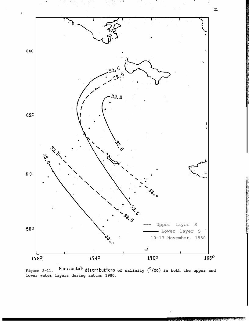
Upper-and lower-layer distributions of salinity (Figure 2-11) show maximum
salinity in both layers near the shelf break and lowest values toward the north-
east.-- ~. .
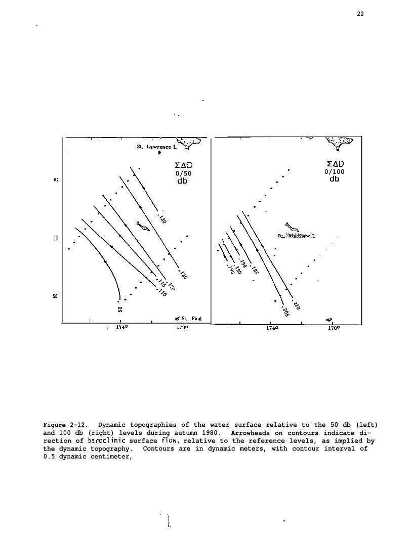
The cross-shelf horizontal density gradient evident in Figures 2-5 and 2-8
suggests that baroclinic northwestward flow may have-been present. Dynamic topo-
graphies of the surface relative to both 50 dbar and 100 dbar (Figure 2-12) con-
firm presence of a weak northwestward baroclinic flow tendency, in agreement with
conventional wisdom concerning circulation on the Bering Sea shelf. The weak
southeasterly counterflow at the southern end of the northwest transect is prob-
ably connected with a bolus of relatively cold (< 2.0 ‘C) water located in the
lower layer (stations 25-28, Figure
2.3.2. February-March 1981
Temperature-salinity data were
a transect which coincided with the. -.
2-6).
acquired, during February-March 1981, along
southeastern of the two transects occupied
. —— .— —--- .——
t
.●
640
62C
(j 00
580
1-
●✎
. .t?3
I
$ ““$N“
“- \
●
●●
\<
●
d+“ o
—–- Upper layer S
. Lower layer S -
10-13 November, 1980“o
d1 I I I
178? 1740 1700 1660
21
Figure 2-11. ‘Horizontald istributions of salinity (O/oo) in both the upper andlower water layers during autumn 1980.
t
22.
62
60
58’
—
,.
\
. ZAD0/50
\= db
.\\ \.””
.s1 I !
+ St. Paul :, 1740 1700
..
..
..
.\ -.
V,. , . . . . . .,., ,. ,:. . “.
EAD0/100db
\
N<SL Matthew I. .
.i .
. ..
.> .
..
Figure 2-12. Dynamic topographies of the water surface relative to the 50 db (left)and 100 db (right) levels during autumn 1980. Arrowheads on contours indicate di-rection of baroclinic surface flow, relative to the reference levels, as implied bythe dynamic topography. Contours are in dynamic meters, with contour interval of0.5 dynamic centimeter,
23
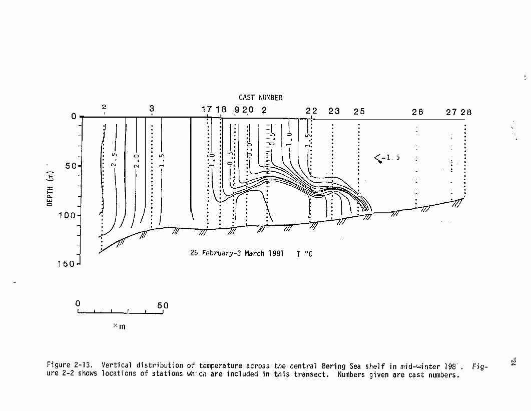
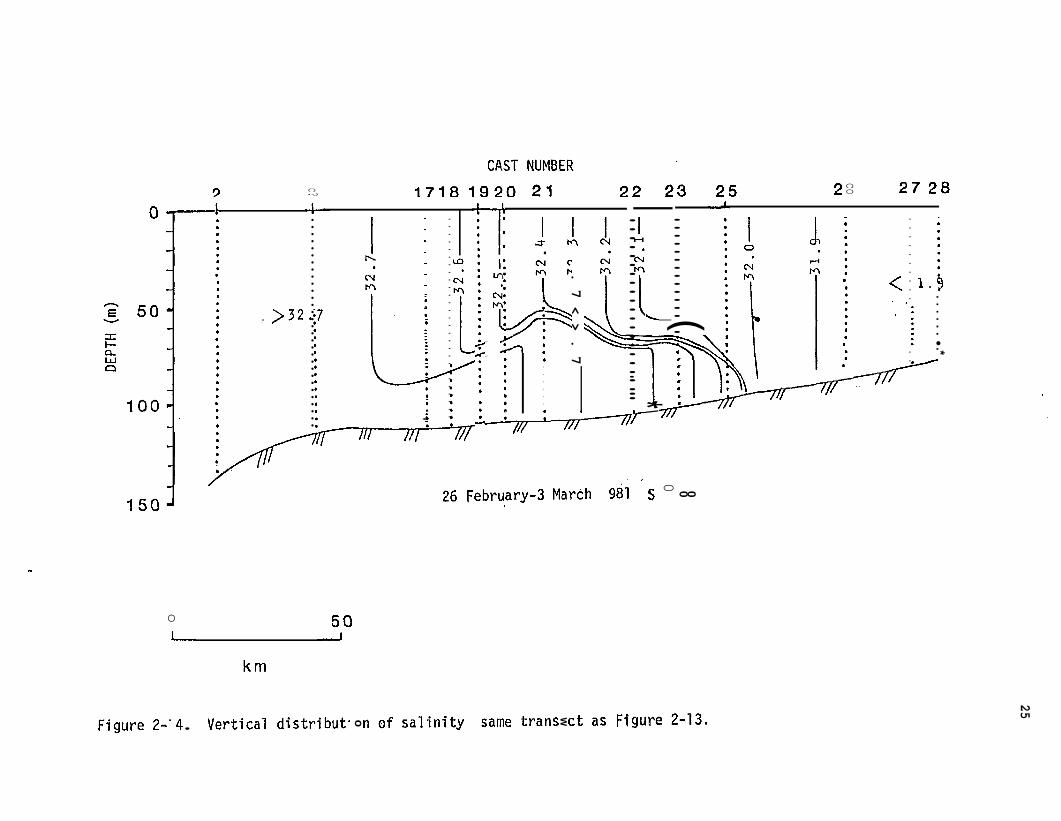
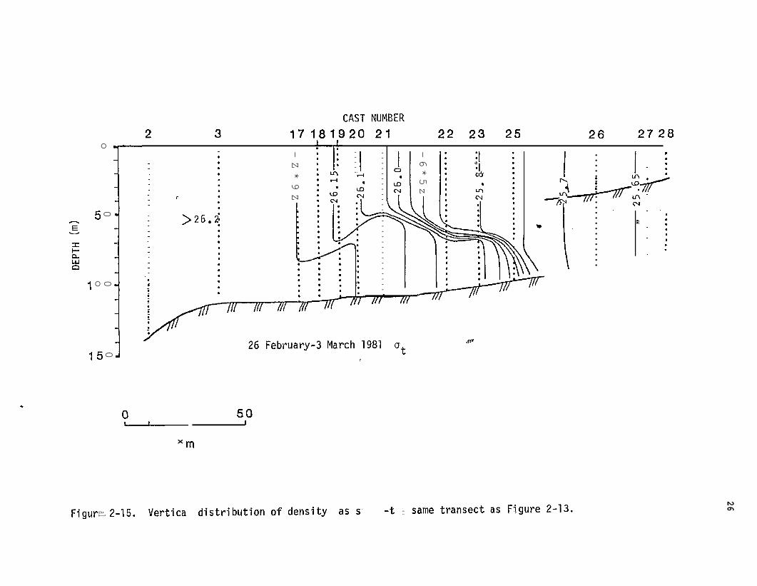
in November 1980 (see Figure 2-l). The vertical distributions of temperature,
salinity and density along th,e transect are shown on Figures 2-13 to 2-15.
Stations 1-20 along this transect were south of the ice edge, while the remaining
stations were occupied after the ice had been forced northward by strong south
winds associat~d with a storm system. The temperature, salinity and density were
near-homogeneous in the vertical in the southern part of the transect. In its
northern portion, the water W%S vertically homogeneous, at or near the freezing
point and had a salinity of about 31.9 O/oo. A region about 80-km wide underlay
the southern extreme location of the ice edge and was characterized by two-layered
water structure. The lower layer was warmer (~ 1.0 ‘C) and more saline (32.5-
32.7 O/oo) than the upper layer (< 0.5 ‘C and 32.1-32.6 O/oo}. The lower layer
was continuous in temperature and salinity properties with water to the south;
that of the upper layer with water to the north.
Two separate occupations were obtained along part of the transect shown in
Figures 2-13 to 2-15. These separate occupations documented variation in the
water column during passage over the region of a severe storm having south winds
which forced the ice edge northward. Temperature is well correlated with salinity
and density (Figures 2-13 to 2-15) and may be used as a tracer of water proper-
ties. This is done in Figure 2-16, which shows the water structure before and
after passage of the storm along the southern portion of the two-layered struc-
ture which underlay the ice edge. Prior to the storm, on 27 February, the lower
layer was well-mixed and the upper layer was stratified. After the storm, on
1 March, both layers were well-mixed and the upper layer had been considerably
deepened at the southern extreme of the two-layered structure. Despite the
r
. ..
“24.
. . . . .
a)ml*aCDalmmlc)olOJCN
. . . . . . . . . . . . . . . . . . . . .
“ \. . . . . . . . . . . . . . . . . . . . .. . . . . . . . . . . . . . . . . . . . . .
.
-@mlav3
In.d+
. - . . . . . . . . . . . . . ...&
EH
5°
-5”o - Jf[
. . . . . . . . . . . . . . .a-
oCu”0,
-Q:::J
y&
-::. . . . . . . . . . . . . . . . .
. .
-b . . .l..
co
r-
*.
r-
c9-
cu -
—-----+
. . . . . . . . . . . . . . . . . . . .. . . .
fp~
~. . . . . . . . . . . . . . . . . . . . . ...*
*. .i
. ...*..... . . . . . . . . . . . . . . . . . .
‘“z——
——
——
.+
Ex
c
.“
25
(nOJt . . . . . . ..m
. . . . . . . ●
.*.A
\.
. . . . . . . . . . .- ...*.. . .
v:”
t-C$Jcool. . . . . . . . . . . . . . . . . . . . . .
\
Inml
(I / . . ./r . . . . . . . .I
. . . . . . . . . . . . . . . . . . .,
(. . . . . . . . . . . . . . .
000
) ll\l—
——
—\
u)—
1.z
s~
M. . . . . . . . . . . . . . . . . . ● . ...*1’
““Gm
LL#.z
[[
. . . . . . .
04CN
—c
.7<>.7
vwas2Gv
1%.
. .
.. Y
..2Y
..
\\
..-.. *.. ””””” ”””””\”} ””””” ”””l9“zs-\P
. . . . . . . . . . . . . . . . . . . . . . . . . . .
-J[. . . . . . . . . . ...-===. .= . . . ..-
● *—L.
zc
. . . . . . . . . . . . . . . . . . . . . . . . . . . . . .
so0
c?tn.r-
-0
\. . . . . . . . . . . . . . . . . . . . . . . . . . . . . . . . . . .
●
e.Alo
I
26
U3CIJ
CYmmOJ031-
bT-
m
. . . . . . . . . . . . . . . . . . . .
\“ . . . . . . . . . . . . . . . . . . . .—s9
”s2
“
. . . . . . . . . . . . . . . . . . . . . .
—L
”sz~
#
. . . . . . . . . . . . . . . . . .
R,+3” <Z..-..
—6*5z
—O*9Z
. . . . . . . . . . . .. . . . . . . . . . . . . .
—T-9Z
. . . . .
—Z*9Z
. . . . . . . . . . . . . . . . . . . . . . . . . .mm“K
\.
.k. . . . . . . . . . . . . . . . . . . . . . . . . . . . . . . . . . .L
llialllt?
llll bo
00
0u)
oU2
vT
-
(LIJ) HJd~a
0.mJOJ
Ex
.4
1
Wla.alL3m
.
0 “
%’
~ 50 -E
100
CAST NUMBER3 4 7 8 91011121]~1 16 5 6
I I I I I I I I 1 I I I I
\,< ,,,,,,,,,,,
II
<~
‘(I ‘2 T (°C)
I
\
“ 0>I - 0 . 5I rI II
0.5 c1 * o-1I l .(-J----- 1 0 10 20I I
I2 6
km- 2 7 ;EBRUARY 1981 : w
II I
i//I Ii! / / /
I//~ I /// /~’ I
I II CAST NUMBER
:17 ~a 19 20 ’21Or
2 2
50 -
100 -
\l*(l1 MARCH 1981
‘ - - 1 * 5
I
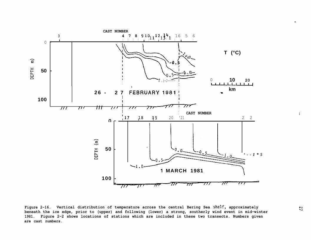
Figure 2-16. Vertical distribution of temperature across the central Bering Sea shelf, approximatelybeneath the ice edge, prior to (upper) and following (lower) a strong, southerly wind event in mid-winter
IVw
1981. Figure 2-2 shows locations of stations which are included in these two transects. Numbers givenare cast numbers.
.
●
.—.28
obvious change in structure, however, the locations where isotherms intersected
the surface at the south edge (the 1.0 “C isotherm) did not shift more than about
20 km northward during the period when the ice edge itsel
100 km to the north. Moreover, the vertical heat content
did not change significantly during the storm event. It
was forced about
of the water column
s concluded that the
change in structure between 27 February and 1 March was due to wind mixing of
the upper layer and its subs+ent deepening due to erosion of the pycnocline.
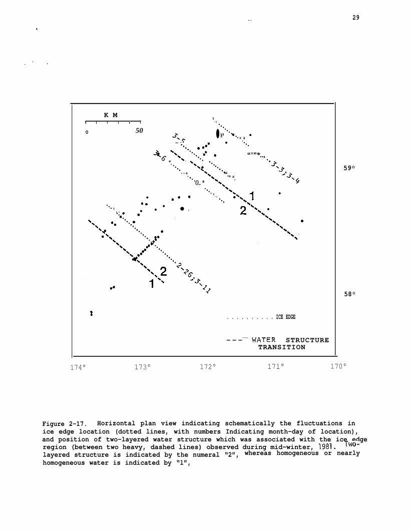
The transitions between vertically homogeneous water (to the north) and
near-homogeneous water (to the south) and the two-layered structtire are compared
in Figure 2-17 with ice edge locations. This figure shows the spatial relation
of the two-layered structure to the ice edge at the various ice edge locations
observed from 26 February-n March 1981.
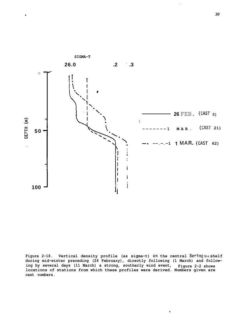
A final example of the observed short-term variability in vertical water
structure is given in Figure 2-18. This shows vertical density profiles at a
station south of the ice “edge” on three separate occupations. The 20 February
structure preceded the storm event, while the 1 March profile directly followed
it and shows-wind-mixing of the upper layer. The 11 March profile shows the
upper layer returning toward its original” (i.e. as observed on 26 February)
stratified state. The change in density in the lower layer was probably advec-
tive in origin, which suggests that some portion of the upper layer variability
was, also, advective rather than due entirely to wind-mixing. Presence to the
southwest of denser lower-layer water suggests that a northward current pulse
might have led to such an increase in density. Data are, however, inadequate to
test this speculation.
Finally, as for the November density structure, that observed in February-
March suggests a baroclinic flow to the northwest. This is confirmed by the
—.
c
.“.
29
K M[ “.,\ \ I b \ “,
o 50 “.,3 ● W* “*.. ●
‘s ●“ .*“..
46 ‘(;”””””.:.;” s “’”*..,%“. “..‘. N ““*.,
““3“, ‘3. . “. %, “., ““J’“.O “.
O.. * ‘% ‘+\\“o. \. ~. ●
● ✎☛☛“., ;\\
“.O ,1**“.. ●
● ● ,“.. - ●#’\\ ●
t . . . . . . . . . . ICE EDGE
- - ---- \4ATER STRUCTURETRANSITION
59°
58°
174° 173° 172° 171° 170°
Figure 2-17. Horizontal plan view indicating schematically the fluctuations inice edge location (dotted lines, with numbers Indicating month-day of location),and position of two-layered water structure which was associated with the ice edgeregion (between two heavy, dashed lines) observed during mid-winter, 1981. Two-layered structure is indicated by the numeral “2”, whereas homogeneous or nearlyhomogeneous water is indicated by “l”,
●
.“
30
SIGMA-T
o
26.0 .2 - .3-
50
100
\●
I I1
1●
I
i
i
i
26 FEB. (CAST 5)I
- - - - - - - 1 M A R . (CAST 21)
–. —-.-.-1 1 MAFL (CAST 62)
Figure 2-18. Vertical density profile (as sigma-t) on the central Bering Sea shelfduring mid-winter preceding (26 February), directly following (1 March) and follow-ing by several days (11 March) a strong, southerly wind event, Figure 2-2 showslocations of stations from which these profiles were derived. Numbers given arecast numbers.
t
——. . 31+
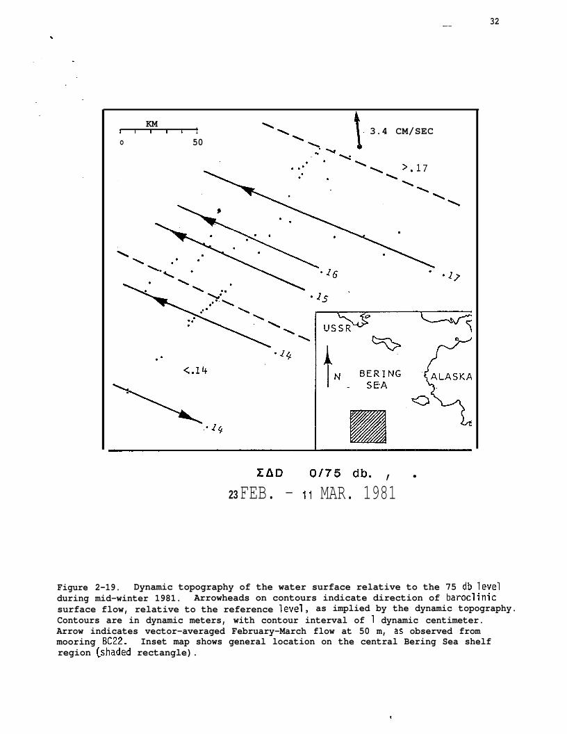
dynamic topography of the surface relative to 75 db (Figure 2-19). The computed
surface current speed, assuming 75 db as.,a level of no motion, was about 7 cm/sec
toward the northwest and was ’confined to the area bounded by the two-layered
structure. This baroclinic flow will be discussed at greater length in Sections
2.4 and 2.5 below.
2.3.3. Temperature-Salinity Characteristics@
The central Bering Sea shelf region was characterized, both in autumn 1980
and mid-winter 1981, by a vertical structure” which was two-layered in temperature
and salinity. In autumn, this structure covered the shelf from the shelf break
to north of the 50-m bottom isobath. In mid-winter, this layered structure
was confined to a “band” approx”
tion of the ice edge.
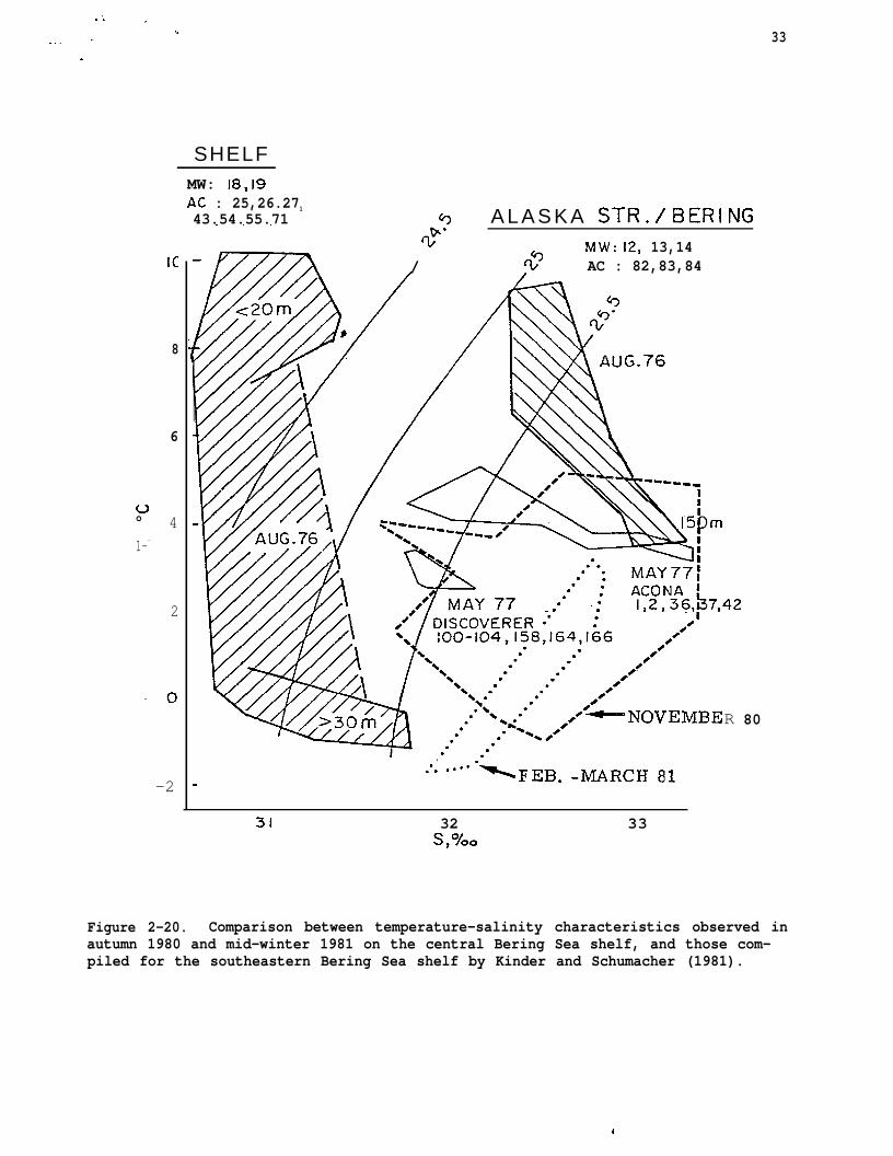
The observed temperature and
those elsewhere in the Bering Sea
diagram constructed by Kinder and
mately 100 km in width which under”ay the loca-
salinity characteristics can be compared with
region by plotting-them superimposed on the
Schumacher (1981) to illustrate Bering Sea
temperature-salinity relationships (Figure 2-20). It is readily apparent that
observed salinities were, for both seasons during which data were obtained, more
characteristic of Alaska Stream/Bering Sea Water than Bering Shelf Water. Tem-
peratures were lower than those typical of Alaska Stream/Bering Water, but our
data were obtained later in the season than that analyzed by Kinder and Schumacher
and so would have been subject to greater cooling. The February-March data were
similar in salinity to the November 1980 data, but minimum observed temperatures
were lower (-1.7 ‘C) as would be expected for winter as compared to autumn data.
In summary, temperature and salinity data obtained during autumn 1980 and mid-
winter 1981 suggest that water on the central Bering Sea shelf has characteristics
——
KM \1 I I I i 1- \
3.4 CM/SECo 50 \
.“ \. k
EAD 0/75 db. , .23 FEB. - 11 MAR. 1981
32
Figure 2-19. Dynamic topography of the water surface relative to the 75 db levelduring mid-winter 1981. Arrowheads on contours indicate direction of baroclinicsurface flow, relative to the reference level, as implied by the dynamic topography.Contours are in dynamic meters, with contour interval of 1 dynamic centimeter.Arrow indicates vector-averaged February-March flow at 50 m, as observed frommooring BC22. Inset map shows general location on the central Bering Sea shelfregion (shaded rectangle).
.
Ic
8
6
uo 4
1--
2
0
-2
33
SHELFMW: 18,19AC : 25,26.271
43.54.55.71 * A L A S K A STR. \8ERl NG. . .t=;‘b MW: 12, 13,14
-Y//~~ /+ AC : 82,83,84
;.76
k“----iI
15~m
42
R
..“. ..”” “-FEB. _~RcH gl
—31 32 33
S,’YOO
80
Figure 2-20. Comparison between temperature-salinity characteristics observed inautumn 1980 and mid-winter 1981 on the central Bering Sea shelf, and those com-piled for the southeastern Bering Sea shelf by Kinder and Schumacher (1981).
I
—.. 34.
more typical of Alaska Stream/Bering Sea Water than of that classified by Kinder
and Schumacher (1981) as Shelf water farther to the southeast. This difference
was due to a large (1-1.5 O/oo) salinity difference betw~en waters on the south-
east and on the central Bering Sea shelf. Speculation concerning this observa-
tion is presented in Section 2.5 below.
35
2.4. CURRENT OBSERVATIONS
Two current records, each more than 200 days in length, were obtained from
50-m depths on the central Bering Sea shelf between November 1980 and June 1981.
Geographical locations of these current records are shown on Figure 2-1; other
pertinent information is listed in Table 2-3.
Both of the overwinter 1~80-81 current records supported
mean, northwesterly flow along the central Bering Sea shelf.
current for the entire record at mooring BC22 was 2.3 cm/see,
the
The
concept of a
vector-averaged
directed toward
340 ‘T. That from mooring BC26 was 3.3 cm/see, directed toward 347 ‘T. These
directions closely approximated the local trend of the isobaths. Speeds were
somewhat higher than the approximately 1 cm/sec means given by
Schumacher (1981b) for the mid-shelf regime farther southeast.
Kinder and
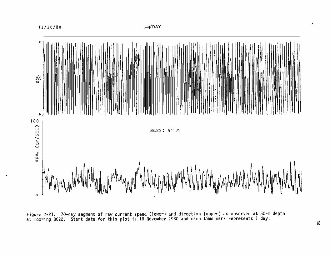
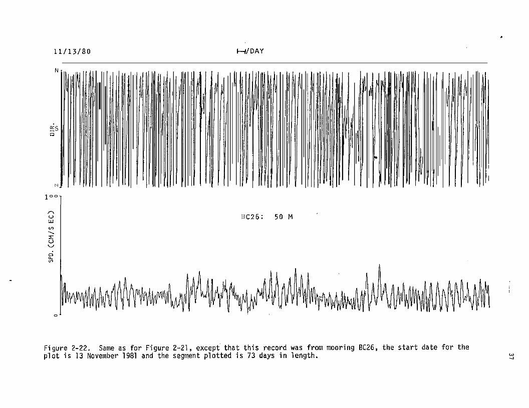
The high-frequency components of flow at both moorings BC22 and BC26 were
heavily dominated by tidal currents which were mixedj predominantly-diurnal.
These show clearly in the time-series segment of raw current data presented in
Figures 2-21 (for BC22) and 2-22 (for BC26). Visual inspection of these time
series reveals tidal currents varying between about 20 to 40 cm/sec at BC22 and
10 to 30 cm/sec at BC26. This decrease in tidal current speeds between BC22 and
BC26 is in qualitative
diurnal tidal currents
agreement with Pearson et al. (1981), who indicate that
decrease in magnitude toward the western Bering Sea shelf.
While the tidal currents were the highest speed components, lower frequency
(1 to 10 day period) fluctuations in speed and direction were evident throughout
the observation period. The tidal signal has”been removed from the current vec-
tors in Figure 2-23 in order to illustrate these fluctuations. Time scales were
of order 7 to 10 days, and reversals to southeastward flow occurred and were more
36
—
0In%
. .Nm0ccl—
_—
—
—.=
=.
-—-.“$10
zg (33s/w3)
“ads
o
d
—..
37
——
~—
——
. .—
—.-
.—
—
—
——
.
“YIOz-00l-l
. .aNvm(32 S/W3)
“GcIS0
.u
[email protected] .2LS*
mo
*
b
BC22: 50 M
BC26: 50 M
~DEC JAN FEB MAR APR h14Y ‘
11/10/80
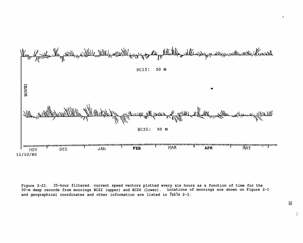
Figure 2-23. 35-hour filtered. current speed vectors plotted every six hours as a function of time for the50-m deep records from moorings BC22 (upper) and BC26 (lower). Locations of moorings are shown on Figure 2-1and geographical coordinates and other information are listed in Table 2-3.
b.)02
.,..
——. . “ 39
frequent later in the record than near its beginning. These fluctuations are
a“lso apparent on the raw speed records (Figures 2-21 and 2-22), with the tidal
currents appearing as high-frequency “noise” superimposed on the lower-frequency
p u l s e . —
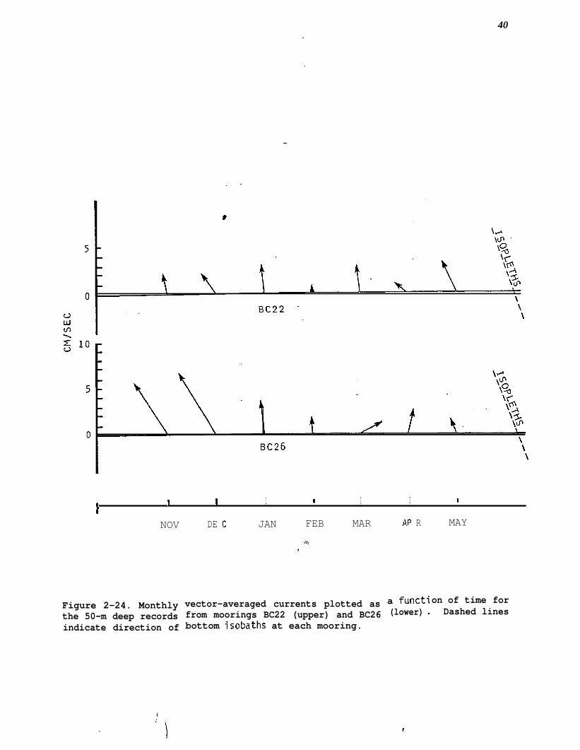
In an attempt to estimate the significance of low-frequency (periods of 10
days or longer) flow fluctuations, monthly vector-averaged currents’were computed
for both moorings and are pr~ented in Figure 2-24. While flow was northerly
during all months, significant variations in east-west flow occurred from month
to month. Comparison with the local bathymetry (shown as the local isobath direc-
tion at each mooring on Figure/2-24) indicates that the flow most strongly paral-
leled the bathymetry in November, December and May at both locations. The great-
est deviation occurred at BC26 in March, when flow was completely across-isobath,
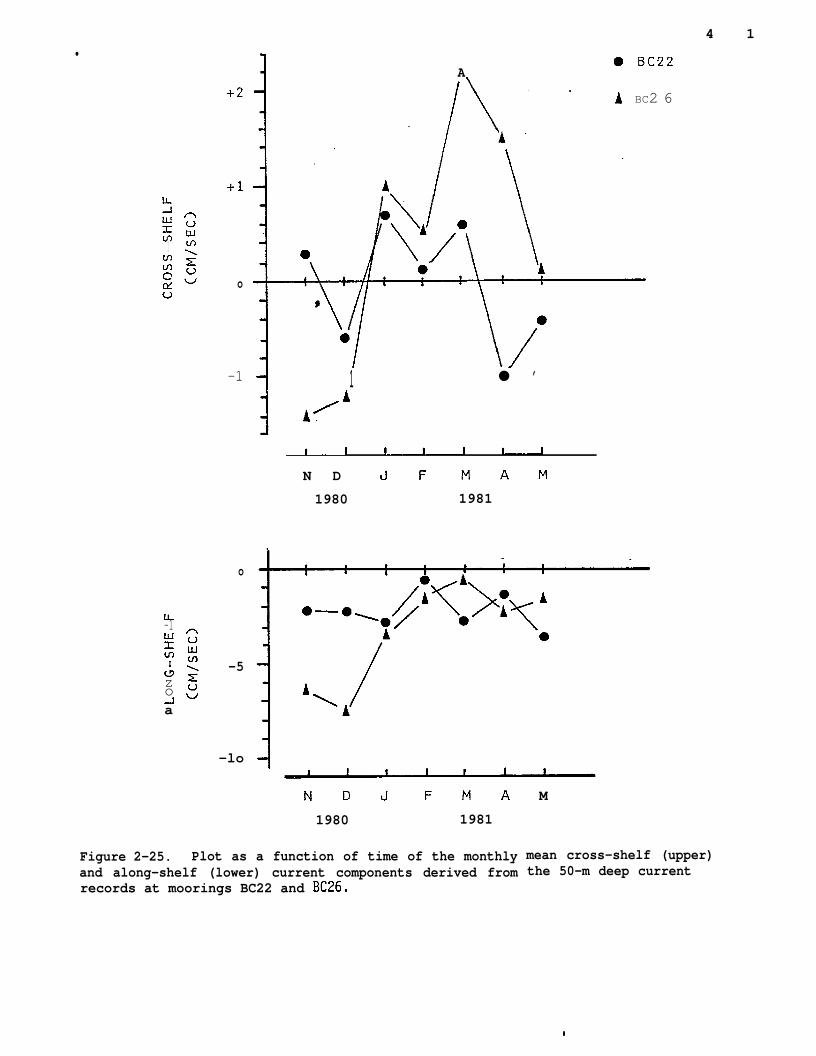
onshore. These
pitted as plots
(Figure 2-25).
time-variations in along- and cross-shelf flow can also be de-
versus time of the monthly mean along- and cross-shelf flow
Along-shelf flow was to the northwest for all months> though it
was minimum through the mid-winter period February-April. Cross-shelf flow
showed a clear tendency at both moorings to be off-shelf (to the southwest)
early and late during the observation period, while flow was onshelf (toward the
northeast) in mid-winter.
Temperature and salinity data obtained during February-March allowed qual-
itative
and the
surface
at 50-m
comparison between the observed February-March currents at mooring BC22
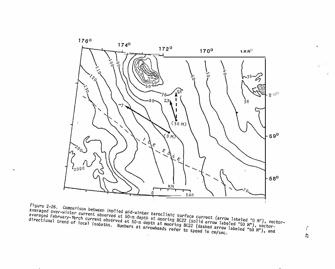
internal density field. Figure 2-26 compares the computed baroclinic
current with both the February-March and over-winter observed currents
depth. The computed surface flow paralleled the ice edge, while the ob-
served current approximately paralleled the bathymetry. Since no current obser-
vations were obtained closer to the surface, it is impossible to rigorously com-
pare magnitudes of the computed baroclinic and observed currents. The component
-.—.-
40
—
I ! I 1 1 I I r
NOV MAYDE C JAN FEB MAR
Q<
Figure 2-24. Monthlythe 50-m deep recordsindicate direction of
vector-averaged currents plotted asfrom moorings BC22 (upper) and BC26bottom isobaths at each mooring.
.AP R
a funct(lower)
on of time forDashed lines
●
A0 BC22
./\””
A BC2 6
A’
LoI
u-)mcCY
+1
ov
-1 1,, ,,, ,,1 ● ’
A/A
N D LIFMAM
1980 1981
L-1
m
Jzo-1a
o
-5
-lo
ND LJFMA
1980 1981
Figure 2-25. Plot as a function of time of the monthlyand along-shelf (lower) current components derived fromrecords at moorings BC22 and BC26.
4 1
M
mean cross-shelf (upper)the 50-m deep current
.“
,.
‘-- 42
#
oac?-
00
00
mm
cou)
u)
/
/’=”n
1
. .
.
I
.“43 “
.— .._
of the observed 50-m current parallel to the ice edge, hence, to the computed
surface current, ”was about 1 cm/sec for February-March. Since this is of the
same order as the computed surface current at the “moorinq (not shown on the fig-
ure), but was at 50-m depth rather than.at the surface, the actual surface flow
may have been somewhat larger than computed due to presence of a barotropic mode.
Further discussion of these currents, within the context of regional oceanographic
processes, is presented below in Section 2.5.s
44
2.5. CONCLUSIONS
2.5.1. Discussion
The most significant contributions resulting from this program have been im-
proved definition of the two-layered temperature and salinity structure associated ~
with the ice edge in mid-winter , and the implications of this structure with re-
spect to time-mean circulatiofi and the ice edge location on the central Bering
Sea shelf. This section will focus primarily upon these aspects of the results.
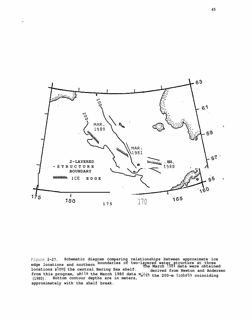
A schematic illustration of the extent of the two-layered structure on the
Bering Sea shelf during mid-winter has been constructed using data obtained in
March 1980 and March 1981 (Figure 2-27). The three crossings of the ice edge
show, even though they were obtained during separate winters, a progressivedi-
vergence toward the west between the actual ice edge and the northern extent of
the two-layered, subsurface water structure. The latter is seen, west of the
Pribilofs, to approximately parallel the 100-m isobath. The ice edge, conversely,
does not parallel the isobaths but extends farther south toward deep water over
the western shelf. Historical analyses of the Bering Sea midwinter ice extent
indicate that this is normally the case (Muench and Ahln~s, 1976; Pease, 1980;
Niebauer, 1981). The ice edge is well north of the shelf break in the eastern
Bering Sea, whereas in the western Bering it extends well south of the shelf break
and overlies deeper water.
The currents observed at 50 m during winter 1980-1981 paralleled isobaths,
whereas the computed baroclinic surface currents paralleled the ice edge rather
than the isobaths. This suggests that the
two-layered structure is controlled by the
isobaths, as observed. On the other hand,
location of the northern edge of the
tendency for local currents to parallel
the computed baroclinic surface flow
..
\
45
0
I’4AR . \
/ “’%%981.-i — S T R U C T U R E \ \“ E19io ,\
1 2-LAYERED \\LUA.U, . . . . MAR.
/ BOUNDARY
~ ICE E D G E
Y’S:’.-,.
I?80 170 165
1 7 5
Figure 2-27. Schematic diagram comparing relationships between approximate iceedge locations and northern boundaries of two-layered water structure at threelocations along the central Bering Sea shelf.
The March 1981 data were obtained
from this program, while the March 1980 data werederived from Newton and Andersen
(1980). Bottom contour depths are in meters, with the 200-m isobath coinciding
approximately with the shelf break.
-.
.-. . 46.
would be somewhat decoupled from the bathymetry by the stratification between
the layers, and would tend to follow a path related to the source of the bare-
clinic field: the melting of ice along the ice edge.
At this point, it is necessary to speculate on processes which might control
the location of the ice edge. In mid-winter, when air temperatures are generally
below freezing, the time mean ice edge location must be controlled primarily by
availability of heat from th~ underlying water column. This heat can be supplied
by advection, or through horizontal and vertical turbulent diffusion. Presence
of a 1-2 cm/sec current component, at 50-m depth, northward normal to the ice edge
suggests one mechanism for advectingh eat beneath the ice. The warm lower layer
is, however, separated from the ice by a colder {approaching the freezing point
at its northern edge), -
layers is about 10-m th-
about 0.2 sigma-t units
than 0.5 sigma-t units 1
ower salinity upper layer. The interface between these
Ck. The density difference between layers varies from
(observed in March 1981) on the central shelf up to more
observed by Newton and Ande&en in March 1980) at the
westernmost section on Figure 2-27. Me hypothesize that, as the upper layer flows
toward the northwest beneath the ice edge, its salinity is decreased by continual
addition of low-salinity water derived from ice melt. This decrease in upper
layer salinity increases the strength of the between-layer density interface, thus
decreasing the upward flux of heat from the relatively warm, lower layer. This
decreased upward heat flux allows the ice to extend farther southward before melt-
ing, as observed. Assuming a mean southward ice advection rate of 20 cm/see,
which is reasonable based both upon data obtained during winter 1981 and upon his-
torical data (Muench and Ahln~s, 1976; Pease, 1980), about
meltwater derived from sea ice is added to the upper layer
and westernmost sections shown on Figure 2-27. This is of
0.5 x 10⁶ m3/sec of
between the easternmost
the same order as the
computed baroclinic flow through the winter 1981 section and, clearly, is suffi-
cient to strongly impact the regional salinity (hence density) field.
“ “47
The westward baroclinic flow associated with the ice edge appears to be a .
. .
consequence of the local input of low-salinity water due to ice melting. It is
this consistent westward flow which leads to the above mechanism allowing the
ice to extend into deeper and deeper water toward the western side of the Bering
shelf. Presence of this baroclinic field and its associated flow also suggests a
reason for the relatively constant location of the two-layered structure, despite
large north-south excursions~of the ice edge. The ice edge excursions occur over
time scales of a few days, as was graphically demonstrated during February-March
1981 (see Figure 2-17). The baroclinic response time of the water column is,
however, longer. It is not likely that the two-layered structure would respond
to single storm events. While it is generally recognized that the year-to-year ‘
variability in maximum southward extent of the ice edge is a function of the
severity of the winter, and that short-term fluctuations in ice extent may occur
in response to discrete storms, it now appears that fluctuations of ice edge lo-
cation over time scales of several weeks are probably damped by the combined re-
sponse time of the baroclinic field associated with the ice edge and the vertical
density structure associated with this field. If ice is advected rapidly southward
over the higher temperature water in the southern part of the two-layered struc-
ture, it will melt and soon return to its original location. On the other hand,
a short term retreat of the ice would place it over
point. Northeasterly winds, which prevail over the
then rapidly advect it southward to its equilibrium
water at or near the freezing
Bering Sea in winter, could
location without appreciable
melting. Freezing of ice in the region overlying the layered structure would re-
lease salt into the water and decrease the density difference across the interface.
This would allow, in turn, increased upward heat flux which would act to slow the
freezing process. Increased melting, conversely, would add low salinity water to
the upper layer, increase the strength of the interface and decrease upward heat
flux available to melt the ice.
48
It was noted above (Section 2.3.3) that water on the central Bering shelf
had temperature-salinity characteristics similar to those of Alaska Stream/Bering
Sea Water rathe~
using data obta-
salinity, which
shelf. Part of
used spring and
than the Bering Shelf !-dater defined by Kinder and Schumacher (1981)
ned farther to the southeast. This difference was due to the
was 1-1.5 O/oo higher on the central than on the southeastern
this difference may have been seasonal, since” Kinder and Schumacher
summer data ~ich would have included maximum freshwater admixture
from terrestrial sources. It also seems reasonable, however, that the flow of
deep layer, oceanic water beneath the ice edge as observed would, through admix-
ture with the upper layers, increase the salinity of the shelf water over that
observed to the southeast.
The above discussion qualitatively relates the observed ice edge location,
currents and the temperature, salinity and density fields on the central Bering
Sea shelf. Quantification and rigorous testing of these hypotheses require addi-
tional field data, particularly with respect to the ~ertical and horizontal defi-
nition of the observed currents, and are beyond the scope of the present treat-
ment.
2.5.2. Summary
The results of the physical oceanographic
port of the overall Bering Sea MIZ program may
investigations carried out in sup-
be summarized as follows:
. The central Bering Sea shelf region was characterized in November 1980and February-March 1981 by a water structure vertically two-layered intemperature, salinity and density. In November, this structure coveredthe entire shelf. In February-March, the structure was restricted to aband about 80-km wide which underlay the ice edge.
● Associated with the two-layered structure in winter was a northwesterlybarocljnic surface current having maximum kpeeds of about-7’cm/sec rela-
tive to the 75 db level. Northwestward baroclinic volume transport rela-tive to the same level was of order 0.5 x 10⁶ m3/sec.
t
. .
49
Observed over-winter mean currents at two locations on the central BeringSea shelf at 50-m depth were 2-3 cm/see, with flow along-isobath to thenorthwest in agreement with conventional wisdom on Bering shelf circula-tion. These mean flow speeds were somewhat higher than those which havebeen previously reported farther to the southeast on the shelf.
Fluctuations, having time scales of 7-10 days, were present in both speedand direction at both current moorings, and led in several instances toreversals to southeastward flow.
Monthly mean obse”rved currents were all alongshelf toward the northwest;however, cross-shelf components fluctuated from month-to-month with max-imum on-shelf flow i% mid-winter.
Tidal currents were 20-40 cm/sec east of St. Matthew Island and were10-30 cm/sec west of it. Tides were mixed, predominantly diurnal.
Overall temperature-salinity characteristics on the central shelf in bothNovember 1980 and February-March 1981 were similar to those of AlaskaStream and Bering Sea Water, rather than to Bering Shelf Water as definedfarther to the southeast.
A hypothesis is developed which qualitatively interrelates the ice edgelocation and the observed temperature, salinity and current fields in-terms of stability of a baroclinic current which is maintained by theice edge, under-ice heat advection by near-bottom flow and control oververtical heat exchange by a density interface.
Acknowledgement
This study was supported by the Bureau of Land
agreement with the National Oceanic and Atmospheric
Management through interagency
Administration, under which a
multiyear program responding to needs of petroleum development of the Alaskan
continental shelf has been managed by the Outer Continental Shelf Environmental
Assessment Program (OCSEAP) Office.
/\
50
References
Clarke, A.J. 1978: On wind-driven quasi-geostrophic water movements near fast-ice edges. Deep-Sea Res. ~, 41-51.
Kinder, T.H. and J.D. Schumacher 1981: Hydrographic structure over the continentalshelf of the southeastern Bering Sea. Chapter 4 in The Eastern Bering SeaShelf: Oceanography and Resources, Volume One (D.W. Hood and J.A. Calder,eds. ), Univ. of Wash. Press, Seattle, 31-52.
Kinder, T.H.” and J.D. Schumacher 1981b: Circulation over the continental shelfof the southeastern Ber&g Sea. Chapter 5 in The Eastern Bering Sea Shelf:Oceanography and Resources, Volume One (D.W. Hood and J.A. Calder, eds.),Univ. of Wash. Press, Seattle, 53-75.
Muench, R.D. and K. Ahlnas 1976: Ice movement and distribution in the BeringSea from March to June 1974. J. Geophys. Res.’8& 4467-4476.
Muench, R.D. and J.D. Schumacher 1980: Physical oceanographic and meteorologicalconditions in the northwest Gulf of Alaska. NOAA Tech. Memo. ERL PMEL-22,147 pp.
Newton, J.L. and B.G. Andersen 1980: MIZPAC 80A; USCG Polar Star (WAGB-1O)Arctic West Operations. March 1980: Bering Sea, Cruise report and prelim-inary oceanographic results. Science Appl. Inc. Report SAI-202-80-460-LJ,La Jolla, Calif., 32 pp. (unpub. man.).
Niebauer, H.J. 1981: Recent fluctuations in sea ice.distribution in.the easternBering Sea. Chapter 9 in The Eastern Bering Sea Shelf: Oceanography andResources, Volume One (D.W. Hood and J.A. Calder, eds.), Univ. of Wash. Press,Seattle, 133-140.
Niebauer, H.J., V. Alexander and R.T. Cooney 1981: Primary production at theeastern Bering Sea ice edge: The physical and biological regimes. Chapter44 in The Eastern Bering Sea Shelf: Oceanography and Resources, Volume Two(D.W. Hood and J.A. Calder, eds.), Univ. of Wash. Press, Seattle 763-772.
Pearson, C.A., H~O. Mofjeld and R.B.” Tripp 1981: Tides of the Eastern Bering SeaShelf. Chapter 8 in The Eastern Bering Sea Shelf: Oceanography and Resources,Volume One (D.W. Hood and J.A. Calder, eds.), Univ. of Wash. Press, Seattle,111-130.
Pease, C.A. 1980: Eastern Bering Sea ice processes. Mo. Wea. Rev. 108, 2015-2023.
I