Embed Size (px)
Citation preview
Physical Modeling in MATLAB®
Allen B. Downey
Version 1.1.6
ii
Physical Modeling in MATLAB®
Copyright 2011 Allen B. Downey
Green Tea Press9 Washburn AveNeedham MA 02492
Permission is granted to copy, distribute, and/or modify this document un-der the terms of the Creative Commons Attribution-NonCommercial 3.0 Un-ported License, which is available at http://creativecommons.org/licenses/by-nc/3.0/.
The original form of this book is LATEX source code. Compiling this code has theeffect of generating a device-independent representation of a textbook, whichcan be converted to other formats and printed.
This book was typeset by the author using latex, dvips and ps2pdf, among otherfree, open-source programs. The LaTeX source for this book is available fromhttp://greenteapress.com/matlab.
MATLAB®is a registered trademark of The Mathworks, Inc. The Mathworksdoes not warrant the accuracy of this book; they probably don’t even like it.
Preface
Most books that use MATLAB are aimed at readers who know how to program.This book is for people who have never programmed before.
As a result, the order of presentation is unusual. The book starts with scalarvalues and works up to vectors and matrices very gradually. This approachis good for beginning programmers, because it is hard to understand compos-ite objects until you understand basic programming semantics. But there areproblems:
� The MATLAB documentation is written in terms of matrices, and so arethe error messages. To mitigate this problem, the book explains the neces-sary vocabulary early and deciphers some of the messages that beginnersfind confusing.
� Many of the examples in the first half of the book are not idiomatic MAT-LAB. I address this problem in the second half by translating the examplesinto a more standard style.
The book puts a lot of emphasis on functions, in part because they are animportant mechanism for controlling program complexity, and also because theyare useful for working with MATLAB tools like fzero and ode45.
I assume that readers know calculus, differential equations, and physics, but notlinear algebra. I explain the math as I go along, but the descriptions might notbe enough for someone who hasn’t seen the material before.
There are small exercises within each chapter, and a few larger exercises at theend of some chapters.
If you have suggestions and corrections, please send them [email protected].
Allen B. DowneyNeedham, MA
iv Preface
Contributor’s list
The following are some of the people who have contributed to this book:
� Michael Lintz spotted the first (of many) typos.
� Kaelyn Stadtmueller reminded me of the importance of linking verbs.
� Roydan Ongie knows a matrix when he sees one (and caught a typo).
� Keerthik Omanakuttan knows that acceleration is not the second deriva-tive of acceleration.
� Pietro Peterlongo pointed out that Binet’s formula is an exact expressionfor the nth Fibonacci number, not an approximation.
� Li Tao pointed out several errors.
� Steven Zhang pointed out an error and a point of confusion in Chapter11.
� Elena Oleynikova pointed out the “gotcha” that script file names can’thave spaces.
� Kelsey Breseman pointed out that numbers as footnote markers can beconfused with exponents, so now I am using symbols.
� Philip Loh sent me some updates for recent revisions of MATLAB.
� Harold Jaffe spotted a typo.
� Vidie Pong pointed out the problem with spaces in filenames.
Contents
Preface iii
1 Variables and values 1
1.1 A glorified calculator . . . . . . . . . . . . . . . . . . . . . . . . 1
1.2 Math functions . . . . . . . . . . . . . . . . . . . . . . . . . . . 2
1.3 Documentation . . . . . . . . . . . . . . . . . . . . . . . . . . . 3
1.4 Variables . . . . . . . . . . . . . . . . . . . . . . . . . . . . . . . 4
1.5 Assignment statements . . . . . . . . . . . . . . . . . . . . . . . 5
1.6 Why variables? . . . . . . . . . . . . . . . . . . . . . . . . . . . 6
1.7 Errors . . . . . . . . . . . . . . . . . . . . . . . . . . . . . . . . 7
1.8 Floating-point arithmetic . . . . . . . . . . . . . . . . . . . . . 8
1.9 Comments . . . . . . . . . . . . . . . . . . . . . . . . . . . . . . 9
1.10 Glossary . . . . . . . . . . . . . . . . . . . . . . . . . . . . . . . 10
1.11 Exercises . . . . . . . . . . . . . . . . . . . . . . . . . . . . . . . 11
2 Scripts 13
2.1 M-files . . . . . . . . . . . . . . . . . . . . . . . . . . . . . . . . 13
2.2 Why scripts? . . . . . . . . . . . . . . . . . . . . . . . . . . . . 14
2.3 The workspace . . . . . . . . . . . . . . . . . . . . . . . . . . . 15
2.4 More errors . . . . . . . . . . . . . . . . . . . . . . . . . . . . . 16
2.5 Pre- and post-conditions . . . . . . . . . . . . . . . . . . . . . . 17
2.6 Assignment and equality . . . . . . . . . . . . . . . . . . . . . . 17
vi Contents
2.7 Incremental development . . . . . . . . . . . . . . . . . . . . . . 18
2.8 Unit testing . . . . . . . . . . . . . . . . . . . . . . . . . . . . . 19
2.9 Glossary . . . . . . . . . . . . . . . . . . . . . . . . . . . . . . . 20
2.10 Exercises . . . . . . . . . . . . . . . . . . . . . . . . . . . . . . . 20
3 Loops 23
3.1 Updating variables . . . . . . . . . . . . . . . . . . . . . . . . . 23
3.2 Kinds of error . . . . . . . . . . . . . . . . . . . . . . . . . . . . 24
3.3 Absolute and relative error . . . . . . . . . . . . . . . . . . . . . 24
3.4 for loops . . . . . . . . . . . . . . . . . . . . . . . . . . . . . . . 25
3.5 plotting . . . . . . . . . . . . . . . . . . . . . . . . . . . . . . . 26
3.6 Sequences . . . . . . . . . . . . . . . . . . . . . . . . . . . . . . 27
3.7 Series . . . . . . . . . . . . . . . . . . . . . . . . . . . . . . . . 28
3.8 Generalization . . . . . . . . . . . . . . . . . . . . . . . . . . . . 28
3.9 Glossary . . . . . . . . . . . . . . . . . . . . . . . . . . . . . . . 29
3.10 Exercises . . . . . . . . . . . . . . . . . . . . . . . . . . . . . . . 30
4 Vectors 33
4.1 Checking preconditions . . . . . . . . . . . . . . . . . . . . . . . 33
4.2 if . . . . . . . . . . . . . . . . . . . . . . . . . . . . . . . . . . 34
4.3 Relational operators . . . . . . . . . . . . . . . . . . . . . . . . 35
4.4 Logical operators . . . . . . . . . . . . . . . . . . . . . . . . . . 35
4.5 Vectors . . . . . . . . . . . . . . . . . . . . . . . . . . . . . . . . 36
4.6 Vector arithmetic . . . . . . . . . . . . . . . . . . . . . . . . . . 37
4.7 Everything is a matrix . . . . . . . . . . . . . . . . . . . . . . . 37
4.8 Indices . . . . . . . . . . . . . . . . . . . . . . . . . . . . . . . . 39
4.9 Indexing errors . . . . . . . . . . . . . . . . . . . . . . . . . . . 40
4.10 Vectors and sequences . . . . . . . . . . . . . . . . . . . . . . . 41
4.11 Plotting vectors . . . . . . . . . . . . . . . . . . . . . . . . . . . 42
4.12 Reduce . . . . . . . . . . . . . . . . . . . . . . . . . . . . . . . . 42
Contents vii
4.13 Apply . . . . . . . . . . . . . . . . . . . . . . . . . . . . . . . . 43
4.14 Search . . . . . . . . . . . . . . . . . . . . . . . . . . . . . . . . 43
4.15 Spoiling the fun . . . . . . . . . . . . . . . . . . . . . . . . . . . 45
4.16 Glossary . . . . . . . . . . . . . . . . . . . . . . . . . . . . . . . 45
4.17 Exercises . . . . . . . . . . . . . . . . . . . . . . . . . . . . . . . 46
5 Functions 49
5.1 Name Collisions . . . . . . . . . . . . . . . . . . . . . . . . . . . 49
5.2 Functions . . . . . . . . . . . . . . . . . . . . . . . . . . . . . . 50
5.3 Documentation . . . . . . . . . . . . . . . . . . . . . . . . . . . 51
5.4 Function names . . . . . . . . . . . . . . . . . . . . . . . . . . . 52
5.5 Multiple input variables . . . . . . . . . . . . . . . . . . . . . . 53
5.6 Logical functions . . . . . . . . . . . . . . . . . . . . . . . . . . 54
5.7 An incremental development example . . . . . . . . . . . . . . . 55
5.8 Nested loops . . . . . . . . . . . . . . . . . . . . . . . . . . . . . 56
5.9 Conditions and flags . . . . . . . . . . . . . . . . . . . . . . . . 57
5.10 Encapsulation and generalization . . . . . . . . . . . . . . . . . 58
5.11 A misstep . . . . . . . . . . . . . . . . . . . . . . . . . . . . . . 60
5.12 continue . . . . . . . . . . . . . . . . . . . . . . . . . . . . . . 61
5.13 Mechanism and leap of faith . . . . . . . . . . . . . . . . . . . . 62
5.14 Glossary . . . . . . . . . . . . . . . . . . . . . . . . . . . . . . . 63
5.15 Exercises . . . . . . . . . . . . . . . . . . . . . . . . . . . . . . . 63
6 Zero-finding 65
6.1 Why functions? . . . . . . . . . . . . . . . . . . . . . . . . . . . 65
6.2 Maps . . . . . . . . . . . . . . . . . . . . . . . . . . . . . . . . . 65
6.3 A note on notation . . . . . . . . . . . . . . . . . . . . . . . . . 66
6.4 Nonlinear equations . . . . . . . . . . . . . . . . . . . . . . . . 66
6.5 Zero-finding . . . . . . . . . . . . . . . . . . . . . . . . . . . . . 68
6.6 fzero . . . . . . . . . . . . . . . . . . . . . . . . . . . . . . . . 69
viii Contents
6.7 What could go wrong? . . . . . . . . . . . . . . . . . . . . . . . 71
6.8 Finding an initial guess . . . . . . . . . . . . . . . . . . . . . . . 72
6.9 More name collisions . . . . . . . . . . . . . . . . . . . . . . . . 73
6.10 Debugging in four acts . . . . . . . . . . . . . . . . . . . . . . . 74
6.11 Glossary . . . . . . . . . . . . . . . . . . . . . . . . . . . . . . . 75
6.12 Exercises . . . . . . . . . . . . . . . . . . . . . . . . . . . . . . . 76
7 Functions of vectors 79
7.1 Functions and files . . . . . . . . . . . . . . . . . . . . . . . . . 79
7.2 Physical modeling . . . . . . . . . . . . . . . . . . . . . . . . . . 80
7.3 Vectors as input variables . . . . . . . . . . . . . . . . . . . . . 81
7.4 Vectors as output variables . . . . . . . . . . . . . . . . . . . . 82
7.5 Vectorizing your functions . . . . . . . . . . . . . . . . . . . . . 82
7.6 Sums and differences . . . . . . . . . . . . . . . . . . . . . . . . 84
7.7 Products and ratios . . . . . . . . . . . . . . . . . . . . . . . . . 85
7.8 Existential quantification . . . . . . . . . . . . . . . . . . . . . . 85
7.9 Universal quantification . . . . . . . . . . . . . . . . . . . . . . 86
7.10 Logical vectors . . . . . . . . . . . . . . . . . . . . . . . . . . . 87
7.11 Glossary . . . . . . . . . . . . . . . . . . . . . . . . . . . . . . . 88
8 Ordinary Differential Equations 89
8.1 Differential equations . . . . . . . . . . . . . . . . . . . . . . . . 89
8.2 Euler’s method . . . . . . . . . . . . . . . . . . . . . . . . . . . 90
8.3 Another note on notation . . . . . . . . . . . . . . . . . . . . . 91
8.4 ode45 . . . . . . . . . . . . . . . . . . . . . . . . . . . . . . . . 92
8.5 Multiple output variables . . . . . . . . . . . . . . . . . . . . . 94
8.6 Analytic or numerical? . . . . . . . . . . . . . . . . . . . . . . . 95
8.7 What can go wrong? . . . . . . . . . . . . . . . . . . . . . . . . 96
8.8 Stiffness . . . . . . . . . . . . . . . . . . . . . . . . . . . . . . . 98
8.9 Glossary . . . . . . . . . . . . . . . . . . . . . . . . . . . . . . . 99
8.10 Exercises . . . . . . . . . . . . . . . . . . . . . . . . . . . . . . . 100
Contents ix
9 Systems of ODEs 103
9.1 Matrices . . . . . . . . . . . . . . . . . . . . . . . . . . . . . . . 103
9.2 Row and column vectors . . . . . . . . . . . . . . . . . . . . . . 104
9.3 The transpose operator . . . . . . . . . . . . . . . . . . . . . . . 105
9.4 Lotka-Voltera . . . . . . . . . . . . . . . . . . . . . . . . . . . . 106
9.5 What can go wrong? . . . . . . . . . . . . . . . . . . . . . . . . 108
9.6 Output matrices . . . . . . . . . . . . . . . . . . . . . . . . . . 108
9.7 Glossary . . . . . . . . . . . . . . . . . . . . . . . . . . . . . . . 110
9.8 Exercises . . . . . . . . . . . . . . . . . . . . . . . . . . . . . . . 110
10 Second-order systems 113
10.1 Nested functions . . . . . . . . . . . . . . . . . . . . . . . . . . 113
10.2 Newtonian motion . . . . . . . . . . . . . . . . . . . . . . . . . 114
10.3 Freefall . . . . . . . . . . . . . . . . . . . . . . . . . . . . . . . . 115
10.4 Air resistance . . . . . . . . . . . . . . . . . . . . . . . . . . . . 116
10.5 Parachute! . . . . . . . . . . . . . . . . . . . . . . . . . . . . . . 118
10.6 Two dimensions . . . . . . . . . . . . . . . . . . . . . . . . . . . 118
10.7 What could go wrong? . . . . . . . . . . . . . . . . . . . . . . . 120
10.8 Glossary . . . . . . . . . . . . . . . . . . . . . . . . . . . . . . . 122
10.9 Exercises . . . . . . . . . . . . . . . . . . . . . . . . . . . . . . . 122
11 Optimization and Interpolation 125
11.1 ODE Events . . . . . . . . . . . . . . . . . . . . . . . . . . . . . 125
11.2 Optimization . . . . . . . . . . . . . . . . . . . . . . . . . . . . 126
11.3 Golden section search . . . . . . . . . . . . . . . . . . . . . . . . 127
11.4 Discrete and continuous maps . . . . . . . . . . . . . . . . . . . 130
11.5 Interpolation . . . . . . . . . . . . . . . . . . . . . . . . . . . . 131
11.6 Interpolating the inverse function . . . . . . . . . . . . . . . . . 132
11.7 Field mice . . . . . . . . . . . . . . . . . . . . . . . . . . . . . . 134
11.8 Glossary . . . . . . . . . . . . . . . . . . . . . . . . . . . . . . . 135
11.9 Exercises . . . . . . . . . . . . . . . . . . . . . . . . . . . . . . . 135
x Contents
12 Vectors as vectors 137
12.1 What’s a vector? . . . . . . . . . . . . . . . . . . . . . . . . . . 137
12.2 Dot and cross products . . . . . . . . . . . . . . . . . . . . . . . 139
12.3 Celestial mechanics . . . . . . . . . . . . . . . . . . . . . . . . . 140
12.4 Animation . . . . . . . . . . . . . . . . . . . . . . . . . . . . . . 141
12.5 Conservation of Energy . . . . . . . . . . . . . . . . . . . . . . . 142
12.6 What is a model for? . . . . . . . . . . . . . . . . . . . . . . . . 143
12.7 Glossary . . . . . . . . . . . . . . . . . . . . . . . . . . . . . . . 144
12.8 Exercises . . . . . . . . . . . . . . . . . . . . . . . . . . . . . . . 144
Chapter 1
Variables and values
1.1 A glorified calculator
At heart, MATLAB is a glorified calculator. When you start MATLAB youwill see a window entitled MATLAB that contains smaller windows entitledCurrent Directory, Command History and Command Window. The CommandWindow runs the MATLAB interpreter, which allows you to type MATLABcommands, then executes them and prints the result.
Initially, the Command Window contains a welcome message with informationabout the version of MATLAB you are running, followed by a chevron:
>>
which is the MATLAB prompt; that is, this symbol prompts you to enter acommand.
The simplest kind of command is a mathematical expression, which is madeup of operands (like numbers, for example) and operators (like the plus sign,+).
If you type an expression and then press Enter (or Return), MATLAB evalu-ates the expression and prints the result.
>> 2 + 1
ans = 3
Just to be clear: in the example above, MATLAB printed >>; I typed 2 + 1
and then hit Enter, and MATLAB printed ans = 3. And when I say “printed,”I really mean “displayed on the screen,” which might be confusing, but it’s theway people talk.
An expression can contain any number of operators and operands. You don’thave to put spaces between them; some people do and some people don’t.
2 Variables and values
>> 1+2+3+4+5+6+7+8+9
ans = 45
Speaking of spaces, you might have noticed that MATLAB puts some spacebetween ans = and the result. In my examples I will leave it out to save paper.
The other arithmetic operators are pretty much what you would expect. Sub-traction is denoted by a minus sign, -; multiplication by an asterisk, * (some-times pronounced “splat”); division by a forward slash /.
>> 2*3 - 4/5
ans = 5.2000
The order of operations is what you would expect from basic algebra: multi-plication and division happen before addition and subtraction. If you want tooverride the order of operations, you can use parentheses.
>> 2 * (3-4) / 5
ans = -0.4000
When I added the parentheses I also changed the spacing to make the groupingof operands clearer to a human reader. This is the first of many style guidelinesI will recommend for making your programs easier to read. Style doesn’t changewhat the program does; the MATLAB interpreter doesn’t check for style. Buthuman readers do, and the most important human who will read your code isyou.
And that brings us to the First Theorem of debugging:
Readable code is debuggable code.
It is worth spending time to make your code pretty; it will save you time de-bugging!
The other common operator is exponentiation, which uses the ^ symbol, some-times pronounced “carat” or “hat”. So 2 raised to the 16th power is
>> 2^16
ans = 65536
As in basic algebra, exponentiation happens before multiplication and division,but again, you can use parentheses to override the order of operations.
1.2 Math functions
MATLAB knows how to compute pretty much every math function you’ve heardof. It knows all the trigonometric functions; here’s how you use them:
>> sin(1)
ans = 0.8415
1.3 Documentation 3
This command is an example of a function call. The name of the function issin, which is the usual abbreviation for the trigonometric sine. The value inparentheses is called the argument. All the trig functions in MATLAB workin radians.
Some functions take more than one argument, in which case they are separatedby commas. For example, atan2 computes the inverse tangent, which is theangle in radians between the positive x-axis and the point with the given y andx coordinates.
>> atan2(1,1)
ans = 0.7854
If that bit of trigonometry isn’t familiar to you, don’t worry about it. It’s justan example of a function with multiple arguments.
MATLAB also provides exponential functions, like exp, which computes e raisedto the given power. So exp(1) is just e.
>> exp(1)
ans = 2.7183
The inverse of exp is log, which computes the logarithm base e:
>> log(exp(3))
ans = 3
This example also demonstrates that function calls can be nested; that is, youcan use the result from one function as an argument for another.
More generally, you can use a function call as an operand in an expression.
>> sqrt(sin(0.5)^2 + cos(0.5)^2)
ans = 1
As you probably guessed, sqrt computes the square root.
There are lots of other math functions, but this is not meant to be a referencemanual. To learn about other functions, you should read the documentation.
1.3 Documentation
MATLAB comes with two forms of online documentation, help and doc.
The help command works from the Command Window; just type help followedby the name of a command.
>> help sin
SIN Sine of argument in radians.
SIN(X) is the sine of the elements of X.
See also asin, sind.
4 Variables and values
Overloaded functions or methods (ones with the same name in other
directories) help sym/sin.m
Reference page in Help browser
doc sin
Unfortunately, this documentation is not beginner-friendly.
One gotcha is that the name of the function appears in the help page in capitalletters, but if you type it like that in MATLAB, you get an error:
>> SIN(1)
??? Undefined command/function 'SIN'.
Another problem is that the help page uses vocabulary you don’t know yet.For example, “the elements of X” won’t make sense until we get to vectors andmatrices a few chapters from now.
The doc pages are usually better. If you type doc sin, a browser appears withmore detailed information about the function, including examples of how to useit. The examples often use vectors and arrays, so they may not make sense yet,but you can get a preview of what’s coming.
1.4 Variables
One of the features that makes MATLAB more powerful than a calculator isthe ability to give a name to a value. A named value is called a variable.
MATLAB comes with a few predefined variables. For example*, the name pi
refers to the mathematical quantity π, which is approximately
>> pi
ans = 3.1416
And if you do anything with complex numbers, you might find it convenientthat both i and j are predefined as the square root of −1.
You can use a variable name anywhere you can use a number; for example, asan operand in an expression:
>> pi * 3^2
ans = 28.2743
or as an argument to a function:
>> sin(pi/2)
ans = 1
>> exp(i * pi)
ans = -1.0000 + 0.0000i
*Technically pi is a function, not a variable, but for now it’s best to pretend.
1.5 Assignment statements 5
As the second example shows, many MATLAB functions work with complexnumbers. This example demonstrates Euler’s Equality: eiπ = −1.
Whenever you evaluate an expression, MATLAB assigns the result to a variablenamed ans. You can use ans in a subsequent calculation as shorthand for “thevalue of the previous expression”.
>> 3^2 + 4^2
ans = 25
>> sqrt(ans)
ans = 5
But keep in mind that the value of ans changes every time you evaluate anexpression.
1.5 Assignment statements
You can create your own variables, and give them values, with an assignmentstatement. The assignment operator is the equals sign, =.
>> x = 6 * 7
x = 42
This example creates a new variable named x and assigns it the value of theexpression 6 * 7. MATLAB responds with the variable name and the computedvalue.
In every assignment statement, the left side has to be a legal variable name.The right side can be any expression, including function calls.
Almost any sequence of lower and upper case letters is a legal variable name.Some punctuation is also legal, but the underscore, , is the only commonly-usednon-letter. Numbers are fine, but not at the beginning. Spaces are not allowed.Variable names are “case sensitive”, so x and X are different variables.
>> fibonacci0 = 1;
>> LENGTH = 10;
>> first_name = 'allen'
first_name = allen
The first two examples demonstrate the use of the semi-colon, which suppressesthe output from a command. In this case MATLAB creates the variables andassigns them values, but displays nothing.
The third example demonstrates that not everything in MATLAB is a number.A sequence of characters in single quotes is a string.
Although i, j and pi are predefined, you are free to reassign them. It is commonto use i and j for other purposes, but it is probably not a good idea to changethe value of pi!
6 Variables and values
1.6 Why variables?
The most common reasons to use variables are
� To avoid recomputing a value that is used repeatedly. For example, if youare performing computations involving e, you might want to compute itonce and save the result.
>> e = exp(1)
e = 2.7183
� To make the connection between the code and the underlying mathematicsmore apparent. If you are computing the area of a circle, you might wantto use a variable named r:
>> r = 3
r = 3
>> area = pi * r^2
area = 28.2743
That way your code resembles the familiar formula πr2.
� To break a long computation into a sequence of steps. Suppose you areevaluating a big, hairy expression like this:
ans = ((x - theta) * sqrt(2 * pi) * sigma) ^ -1 * ...
exp(-1/2 * (log(x - theta) - zeta)^2 / sigma^2)
You can use an ellipsis to break the expression into multiple lines. Justtype ... at the end of the first line and continue on the next.
But often it is better to break the computation into a sequence of stepsand assign intermediate results to variables.
shiftx = x - theta
denom = shiftx * sqrt(2 * pi) * sigma
temp = (log(shiftx) - zeta) / sigma
exponent = -1/2 * temp^2
ans = exp(exponent) / denom
The names of the intermediate variables explain their role in the compu-tation. shiftx is the value of x shifted by theta. It should be no surprisethat exponent is the argument of exp, and denom ends up in the denom-inator. Choosing informative names makes the code easier to read andunderstand (see the First Theorem of Debugging).
1.7 Errors 7
1.7 Errors
It’s early, but now would be a good time to start making errors. Whenever youlearn a new feature, you should try to make as many errors as possible, as soonas possible.
When you make deliberate errors, you get to see what the error messages looklike. Later, when you make accidental errors, you will know what the messagesmean.
A common error for beginning programmers is leaving out the * for multiplica-tion.
>> area = pi r^2
??? area = pi r^2
|
Error: Unexpected MATLAB expression.
The error message indicates that, after seeing the operand pi, MATLAB was“expecting” to see an operator, like *. Instead, it got a variable name, which isthe “unexpected expression” indicated by the vertical line, | (which is called a“pipe”).
Another common error is to leave out the parentheses around the arguments ofa function. For example, in math notation, it is common to write somethinglike sinπ, but not in MATLAB.
>> sin pi
??? Function 'sin' is not defined for values of class 'char'.
The problem is that when you leave out the parentheses, MATLAB treats theargument as a string (rather than as an expression). In this case the sin functiongenerates a reasonable error message, but in other cases the results can bebaffling. For example, what do you think is going on here?
>> abs pi
ans = 112 105
There is a reason for this “feature”, but rather than get into that now, let mesuggest that you should always put parentheses around arguments.
This example also demonstrates the Second Theorem of Debugging:
The only thing worse than getting an error message is not gettingan error message.
Beginning programmers hate error messages and do everything they can to makethem go away. Experienced programmers know that error messages are yourfriend. They can be hard to understand, and even misleading, but it is worthmaking some effort to understand them.
Here’s another common rookie error. If you were translating the following math-ematical expression into MATLAB:
8 Variables and values
1
2√π
You might be tempted to write something like this:
1 / 2 * sqrt(pi)
But that would be wrong. So very wrong.
1.8 Floating-point arithmetic
In mathematics, there are several kinds of numbers: integer, real, rational,irrational, imaginary, complex, etc. MATLAB only has one kind of number,called floating-point.
You might have noticed that MATLAB expresses values in decimal notation.So, for example, the rational number 1/3 is represented by the floating-pointvalue
>> 1/3
ans = 0.3333
which is only approximately correct. It’s not quite as bad as it seems; MATLABuses more digits than it shows by default. You can change the format to seethe other digits.
>> format long
>> 1/3
ans = 0.33333333333333
Internally, MATLAB uses the IEEE double-precision floating-point format,which provides about 15 significant digits of precision (in base 10). Leadingand trailing zeros don’t count as “significant” digits, so MATLAB can representlarge and small numbers with the same precision.
Very large and very small values are displayed in scientific notation.
>> factorial(100)
ans = 9.332621544394410e+157
The e in this notation is not the transcendental number known as e; it is just anabbreviation for “exponent”. So this means that 100! is approximately 9.33 ×10157. The exact solution is a 158-digit integer, but we only know the first 16digits.
You can enter numbers using the same notation.
>> speed_of_light = 3.0e8
speed_of_light = 300000000
1.9 Comments 9
Although MATLAB can handle large numbers, there is a limit. The predefinedvariables realmax and realmin contain the largest and smallest numbers thatMATLAB can handle�.
>> realmax
ans = 1.797693134862316e+308
>> realmin
ans = 2.225073858507201e-308
If the result of a computation is too big, MATLAB “rounds up” to infinity.
>> factorial(170)
ans = 7.257415615307994e+306
>> factorial(171)
ans = Inf
Division by zero also returns Inf, but in this case MATLAB gives you a warningbecause division by zero is usually considered undefined.
>> 1/0
Warning: Divide by zero.
ans = Inf
A warning is like an error message without teeth; the computation is allowed tocontinue. Allowing Inf to propagate through a computation doesn’t always dowhat you expect, but if you are careful with how you use it, Inf can be quiteuseful.
For operations that are truly undefined, MATLAB returns NaN, which standsfor “not a number”.
>> 0/0
Warning: Divide by zero.
ans = NaN
1.9 Comments
Along with the commands that make up a program, it is useful to includecomments that provide additional information about the program. The percentsymbol % separates the comments from the code.
>> speed_of_light = 3.0e8 % meters per second
speed_of_light = 300000000
�The names of these variables are misleading; floating-point numbers are sometimes,wrongly, called “real”.
10 Variables and values
The comment runs from the percent symbol to the end of the line. In this caseit specifies the units of the value. In an ideal world, MATLAB would keep trackof units and propagate them through the computation, but for now that burdenfalls on the programmer.
Comments have no effect on the execution of the program. They are therefor human readers. Good comments make programs more readable, but badcomments are useless or (even worse) misleading.
Avoid comments that are redundant with the code:
>> x = 5 % assign the value 5 to x
Good comments provide additional information that is not in the code, likeunits in the example above, or the meaning of a variable:
>> p = 0 % position from the origin in meters
>> v = 100 % velocity in meters / second
>> a = -9.8 % acceleration of gravity in meters / second^2
If you use longer variable names, you might not need explanatory comments,but there is a tradeoff: longer code can become harder to read. Also, if you aretranslating from math that uses short variable names, it can be useful to makeyour program consistent with your math.
1.10 Glossary
interpreter: The program that reads and executes MATLAB code.
command: A line of MATLAB code executed by the interpreter.
prompt: The symbol the interpreter prints to indicate that it is waiting foryou to type a command.
operator: One of the symbols, like * and +, that represent mathematical op-erations.
operand: A number or variable that appears in an expression along with op-erators.
expression: A sequence of operands and operators that specifies a mathemat-ical computation and yields a value.
value: The numerical result of a computation.
evaluate: To compute the value of an expression.
order of operations: The rules that specify which operations in an expressionare performed first.
function: A named computation; for example log10 is the name of a functionthat computes logarithms in base 10.
1.11 Exercises 11
call: To cause a function to execute and compute a result.
function call: A kind of command that executes a function.
argument: An expression that appears in a function call to specify the valuethe function operates on.
nested function call: An expression that uses the result from one functioncall as an argument for another.
variable: A named value.
assignment statement: A command that creates a new variable (if necessary)and gives it a value.
string: A value that consists of a sequence of characters (as opposed to a num-ber).
floating-point: The kind of number MATLAB works with. All floating-pointnumbers can be represented with about 16 significant decimal digits (un-like mathematical integers and reals).
scientific notation: A format for typing and displaying large and small num-bers; e.g. 3.0e8, which represents 3.0× 10⁸ or 300,000,000.
comment: Part of a program that provides additional information about theprogram, but does not affect its execution.
1.11 Exercises
Exercise 1.1 Write a MATLAB expression that evaluates the following mathexpression. You can assume that the variables mu, sigma and x already exist.
e−
(
x−µ
σ√
2
)
2
σ√2π
(1.1)
Note: you can’t use Greek letters in MATLAB; when translating math expres-sions with Greek letters, it is common to write out the name of the letter (as-suming you know it).

12 Variables and values
Chapter 2
Scripts
2.1 M-files
So far we have typed all of our programs “at the prompt,” which is fine if youare not writing more than a few lines. Beyond that, you will want to store yourprogram in a script and then execute the script.
A script is a file that contains MATLAB code. These files are also called “M-files” because they use the extension .m, which is short for MATLAB.
You can create and edit scripts with any text editor or word processor, but thesimplest way is by selecting New→Script from the File menu. A window appearsrunning a text editor specially designed for MATLAB.
Type the following code in the editor
x = 5
and then press the (outdated) floppy disk icon, or select Save from the Filemenu.Either way, a dialog box appears where you can choose the file name and thedirectory where it should go. Change the name to myscript.m and leave thedirectory unchanged.
By default, MATLAB will store your script in a directory that is on the searchpath, which is the list of directories MATLAB searches for scripts.
Go back to the Command Window and type myscript (without the extension)at the prompt. MATLAB executes your script and displays the result.
>> myscript
x = 5
When you run a script, MATLAB executes the commands in the M-File, oneafter another, exactly as if you had typed them at the prompt.
If something goes wrong and MATLAB can’t find your script, you will get anerror message like:
14 Scripts
>> myscript
??? Undefined function or variable 'myscript'.
In this case you can either save your script again in a directory that is on thesearch path, or modify the search path to include the directory where you keepyour scripts. You’ll have to consult the documentation for the details (sorry!).
The filename can be anything you want, but you should try to choose somethingmeaningful and memorable. You should be very careful to choose a name that isnot already in use; if you do, you might accidentally replace one of MATLAB’sfunctions with your own. Finally, the name of the file cannot contain spaces. Ifyou create a file named my script.m, MATLAB doesn’t complain until you tryto run it:
>> my script
??? Undefined function or method 'my' for input arguments
of type 'char'.
The problem is that it is looking for a scipt named my. The problem is evenworse if the first word of the filename is a function that exists. Just for fun,create a script named abs val.m and run it.
Keeping track of your scripts can be a pain. To keep things simple, for now, Isuggest putting all of your scripts in the default directory.
Exercise 2.1 The Fibonacci sequence, denoted F , is described by the equationsF1 = 1, F2 = 1, and for i ≥ 3, Fi = Fi−1 +Fi−2. The elements of this sequenceoccur naturally in many plants, particularly those with petals or scales arrangedin the form of a logarithmic spiral.
The following expression computes the nth Fibonacci number:
Fn =1√5
[(
1 +√5
2
)n
−(
1−√5
2
)n]
(2.1)
Translate this expression into MATLAB and store your code in a file namedfibonacci1. At the prompt, set the value of n to 10 and then run your script.The last line of your script should assign the value of Fn to ans. (The correctvalue of F10 is 55).
2.2 Why scripts?
The most common reasons to use scripts are:
� When you are writing more than a couple of lines of code, it might takea few tries to get everything right. Putting your code in a script makes iteasier to edit than typing it at the prompt.
2.3 The workspace 15
On the other hand, it can be a pain to switch back and forth between theCommand Window and the Editor. Try to arrange your windows so youcan see the Editor and the Command Window at the same time, and usethe Tab key or the mouse to switch between them.
� If you choose good names for your scripts, you will be able to rememberwhich script does what, and you might be able to reuse a script from oneproject to the next.
� If you run a script repeatedly, it is faster to type the name of the scriptthan to retype the code!
Unfortunately, the great power of scripts comes with great responsibility, whichis that you have to make sure that the code you are running is the code youthink you are running.
First, whenever you edit your script, you have to save it before you run it. Ifyou forget to save it, you will be running the old version.
Also, whenever you start a new script, start with something simple, like x=5,that produces a visible effect. Then run your script and confirm that you getwhat you expect. MATLAB comes with a lot of predefined functions. It is easyto write a script that has the same name as a MATLAB function, and if youare not careful, you might find yourself running the MATLAB function insteadof your script.
Either way, if the code you are running is not the code you are looking at,you will find debugging a frustrating exercise! And that brings us to the ThirdTheorem of Debugging:
You must always be 100% sure that the code you are running is thecode you think you are running.
2.3 The workspace
The variables you create are stored in the workspace, which is a set of variablesand their values. The who command prints the names of the variables in theworkspace.
>> x=5;
>> y=7;
>> z=9;
>> who
Your variables are:
x y z
16 Scripts
The clear command removes variables.
>> clear y
>> who
Your variables are:
x z
To display the value of a variable, you can use the disp function.
>> disp(z)
9
But it’s easier to just type the variable name.
>> z
z = 9
(Strictly speaking, the name of a variable is an expression, so evaluating itshould assign a value to ans, but MATLAB seems to handle this as a specialcase.)
2.4 More errors
Again, when you try something new, you should make a few mistakes on purposeso you’ll recognize them later.
The most common error with scripts is to run a script without creating thenecessary variables. For example, fibonacci1 requires you to assign a value ton. If you don’t:
>> fibonacci1
??? Undefined function or variable "n".
Error in ==> fibonacci1 at 4
diff = t1^(n+1) - t2^(n+1);
The details of this message might be different for you, depending on what’s inyour script. But the general idea is that n is undefined. Notice that MATLABtells you what line of your program the error is in, and displays the line.
This information can be helpful, but beware! MATLAB is telling you where theerror was discovered, not where the error is. In this case, the error is not in thescript at all; it is, in a sense, in the workspace.
Which brings us to the Fourth Theorem of Debugging:
Error messages tell you where the problem was discovered, not whereit was caused.
The object of the game is to find the cause and fix it—not just to make theerror message go away.
2.5 Pre- and post-conditions 17
2.5 Pre- and post-conditions
Every script should contain a comment that explains what it does, and whatthe requirements are for the workspace. For example, I might put somethinglike this at the beginning of fibonacci1:
% Computes the nth Fibonacci number.
% Precondition: you must assign a value to n before running
% this script. Postcondition: the result is stored in ans.
A precondition is something that must be true, when the script starts, in orderfor it to work correctly. A postcondition is something that will be true whenthe script completes.
If there is a comment at the beginning of a script, MATLAB assumes it isthe documentation for the script, so if you type help fibonacci1, you get thecontents of the comment (without the percent signs).
>> help fibonacci1
Computes the nth Fibonacci number.
Precondition: you must assign a value to n before running
this script. Postcondition: the result is stored in ans.
That way, scripts that you write behave just like predefined scripts. You caneven use the doc command to see your comment in the Help Window.
2.6 Assignment and equality
In mathematics the equals sign means that the two sides of the equation havethe same value. In MATLAB an assignment statement looks like a mathematicalequality, but it’s not.
One difference is that the sides of an assignment statement are not interchange-able. The right side can be any legal expression, but the left side has to be avariable, which is called the target of the assignment. So this is legal:
>> y = 1;
>> x = y+1
x = 2
But this is not:
>> y+1 = x
??? y+1 = x
|
Error: The expression to the left of the equals sign is not a valid
target for an assignment.
In this case the error message is pretty helpful, as long as you know what a“target” is.
18 Scripts
Another difference is that an assignment statement is only temporary, in thefollowing sense. When you assign x = y+1, you get the current value of y. If ychanges later, x does not get updated.
A third difference is that a mathematical equality is a statement that may ormay not be true. For example, y = y + 1 is a statement that happens to befalse for all real values of y. In MATLAB, y = y+1 is a sensible and usefulassignment statement. It reads the current value of y, adds one, and replacesthe old value with the new value.
>> y = 1;
>> y = y+1
y = 2
When you read MATLAB code, you might find it helpful to pronounce theequals sign “gets” rather than “equals.” So x = y+1 is pronounced “x gets thevalue of y plus one.”
To test your understanding of assignment statements, try this exercise:
Exercise 2.2 Write a few lines of code that swap the values of x and y. Putyour code in a script called swap and test it.
2.7 Incremental development
When you start writing scripts that are more than a few lines, you might findyourself spending more and more time debugging. The more code you writebefore you start debugging, the harder it is to find the problem.
Incremental development is a way of programming that tries to minimizethe pain of debugging. The fundamental steps are
1. Always start with a working program. If you have an example from abook or a program you wrote that is similar to what you are working on,start with that. Otherwise, start with something you know is correct, likex=5. Run the program and confirm that you are running the program youthink you are running.
This step is important, because in most environments there are lots oflittle things that can trip you up when you start a new project. Get themout of the way so you can focus on programming.
2. Make one small, testable change at a time. A “testable” change is onethat displays something on the screen (or has some other effect) that youcan check. Ideally, you should know what the correct answer is, or be ableto check it by performing another computation.
3. Run the program and see if the change worked. If so, go back to Step 2.If not, you will have to do some debugging, but if the change you madewas small, it shouldn’t take long to find the problem.

2.8 Unit testing 19
When this process works, you will find that your changes usually work the firsttime, or the problem is obvious. That’s a good thing, and it brings us to theFifth Theorem of Debugging:
The best kind of debugging is the kind you don’t have to do.
In practice, there are two problems with incremental development:
� Sometimes you have to write extra code to generate visible output thatyou can check. This extra code is called scaffolding because you use itto build the program and then remove it when you are done. But timeyou save on debugging is almost always worth the time you spend onscaffolding.
� When you are getting started, it is usually not obvious how to choose thesteps that get from x=5 to the program you are trying to write. There isan extended example in Section 5.7.
If you find yourself writing more than a few lines of code before you starttesting, and you are spending a lot of time debugging, you should try incrementaldevelopment.
2.8 Unit testing
In large software projects, unit testing is the process of testing software com-ponents in isolation before putting them together.
The programs we have seen so far are not big enough to need unit testing, butthe same principle applies when you are working with a new function or a newlanguage feature for the first time. You should test it in isolation before youput it into your program.
For example, suppose you know that x is the sine of some angle and you wantto find the angle. You find the MATLAB function asin, and you are prettysure it computes the inverse sine function. Pretty sure is not good enough; youwant to be very sure.
Since we know sin 0 = 0, we could try
>> asin(0)
ans = 0
which is correct. Also, we know that the sine of 90 degrees is 1, so if we tryasin(1), we expect the answer to be 90, right?
>> asin(1)
ans = 1.5708
20 Scripts
Oops. We forgot that the trig functions in MATLAB work in radians, notdegrees. So the correct answer is π/2, which we can confirm by dividing throughby pi:
>> asin(1) / pi
ans = 0.5000
With this kind of unit testing, you are not really checking for errors in MATLAB,you are checking your understanding. If you make an error because you areconfused about how MATLAB works, it might take a long time to find, becausewhen you look at the code, it looks right.
Which brings us to the Sixth Theorem of Debugging:
The worst bugs aren’t in your code; they are in your head.
2.9 Glossary
M-file: A file that contains a MATLAB program.
script: An M-file that contains a sequence of MATLAB commands.
search path: The list of directories where MATLAB looks for M-files.
workspace: A set of variables and their values.
precondition: Something that must be true when the script starts, in orderfor it to work correctly.
postcondition: Something that will be true when the script completes.
target: The variable on the left side of an assignment statement.
incremental development: A way of programming by making a series ofsmall, testable changes.
scaffolding: Code you write to help you program or debug, but which is notpart of the finished program.
unit testing: A process of testing software by testing each component in iso-lation.
2.10 Exercises
Exercise 2.3 Imagine that you are the owner of a car rental company with twolocations, Albany and Boston. Some of your customers do “one-way rentals,”picking up a car in Albany and returning it in Boston, or the other way around.Over time, you have observed that each week 5% of the cars in Albany are
2.10 Exercises 21
dropped off in Boston, and 3% of the cars in Boston get dropped off in Albany.At the beginning of the year, there are 150 cars at each location.
Write a script called car update that updates the number of cars in each locationfrom one week to the next. The precondition is that the variables a and b
contain the number of cars in each location at the beginning of the week. Thepostcondition is that a and b have been modified to reflect the number of carsthat moved.
To test your program, initialize a and b at the prompt and then execute thescript. The script should display the updated values of a and b, but not anyintermediate variables.
Note: cars are countable things, so a and b should always be integer values. Youmight want to use the round function to compute the number of cars that moveduring each week.
If you execute your script repeatedly, you can simulate the passage of time fromweek to week. What do you think will happen to the number of cars? Will allthe cars end up in one place? Will the number of cars reach an equilibrium, orwill it oscillate from week to week?
In the next chapter we will see how to execute your script automatically, andhow to plot the values of a and b versus time.

22 Scripts
Chapter 3
Loops
3.1 Updating variables
In Exercise 2.3, you might have been tempted to write something like
a = a - 0.05*a + 0.03*b
b = b + 0.05*a - 0.03*b
But that would be wrong, so very wrong. Why? The problem is that the firstline changes the value of a, so when the second line runs, it gets the old valueof b and the new value of a. As a result, the change in a is not always the sameas the change in b, which violates the principle of Conversation of Cars!
One solution is to use temporary variables anew and bnew:
anew = a - 0.05*a + 0.03*b
bnew = b + 0.05*a - 0.03*b
a = anew
b = bnew
This has the effect of updating the variables “simultaneously;” that is, it readsboth old values before writing either new value.
The following is an alternative solution that has the added advantage of simpli-fying the computation:
atob = 0.05*a - 0.03*b
a = a - atob
b = b + atob
It is easy to look at this code and confirm that it obeys Conversation of Cars.Even if the value of atob is wrong, at least the total number of cars is right.And that brings us to the Seventh Theorem of Debugging:
The best way to avoid a bug is to make it impossible.
In this case, removing redundancy also eliminates the opportunity for a bug.
24 Loops
3.2 Kinds of error
There are four kinds of error:
Syntax error: You have written a MATLAB command that cannot executebecause it violates one of the rules of syntax. For example, you can’t havetwo operands in a row without an operator, so pi r^2 contains a syntaxerror. When MATLAB finds a syntax error, it prints an error messageand stops running your program.
Runtime error: Your program starts running, but something goes wrongalong the way. For example, if you try to access a variable that doesn’texist, that’s a runtime error. When MATLAB detects the problem, itprints an error message and stops.
Logical error: Your program runs without generating any error messages, butit doesn’t do the right thing. The problem in the previous section, wherewe changed the value of a before reading the old value, is a logical error.
Numerical error: Most computations in MATLAB are only approximatelyright. Most of the time the errors are small enough that we don’t care,but in some cases the roundoff errors are a problem.
Syntax errors are usually the easiest. Sometimes the error messages are confus-ing, but MATLAB can usually tell you where the error is, at least roughly.
Run time errors are harder because, as I mentioned before, MATLAB can tellyou where it detected the problem, but not what caused it.
Logical errors are hard because MATLAB can’t help at all. Only you know whatthe program is supposed to do, so only you can check it. From MATLAB’s pointof view, there’s nothing wrong with the program; the bug is in your head!
Numerical errors can be tricky because it’s not clear whether the problem isyour fault. For most simple computations, MATLAB produces the floating-point value that is closest to the exact solution, which means that the first 15significant digits should be correct. But some computations are ill-conditioned,which means that even if your program is correct, the roundoff errors accumulateand the number of correct digits can be smaller. Sometimes MATLAB can warnyou that this is happening, but not always! Precision (the number of digits inthe answer) does not imply accuracy (the number of digits that are right).
3.3 Absolute and relative error
There are two ways of thinking about numerical errors, called absolute andrelative.
3.4 for loops 25
An absolute error is just the difference between the correct value and the ap-proximation. We usually write the magnitude of the error, ignoring its sign,because it doesn’t matter whether the approximation is too high or too low.
For example, we might want to estimate 9! using the formula√18π(9/e)9. The
exact answer is 9 · 8 · 7 · 6 · 5 · 4 · 3 · 2 · 1 = 362, 880. The approximation is359, 536.87. The absolute error is 3,343.13.
At first glance, that sounds like a lot—we’re off by three thousand—but it isworth taking into account the size of the thing we are estimating. For example,$3000 matters a lot if we are talking about my annual salary, but not at all ifwe are talking about the national debt.
A natural way to handle this problem is to use relative error, which is the errorexpressed as a fraction (or percentage) of the exact value. In this case, wewould divide the error by 362,880, yielding .00921, which is just less than 1%.For many purposes, being off by 1% is good enough.
3.4 for loops
A loop is a part of a program that executes repeatedly; a for loop is the kindof loop that uses the for statement.
The simplest use of a for loop is to execute one or more lines a fixed numberof times. For example, in the last chapter we wrote a script named car update
that simulates one week in the life of a rental car company. To simulate anentire year, we have to run it 52 times:
for i=1:52
car_update
end
The first line looks like an assignment statement, and it is like an assignmentstatement, except that it runs more than once. The first time it runs, it createsthe variable i and assigns it the value 1. The second time, i gets the value 2,and so on, up to 52.
The colon operator, :, specifies a range of integers. In the spirit of unit testing,you can create a range at the prompt:
>> 1:5
ans = 1 2 3 4 5
The variable you use in the for statement is called the loop variable. It is acommon convention to use the names i, j and k as loop variables.
The statements inside the loop are called the body. By convention, they areindented to show that they are inside the loop, but the indentation does notactually affect the execution of the program. The end of the loop is officiallymarked by the end statement.
To see the loop in action you can run a loop that displays the loop variable:
26 Loops
>> for i=1:5
i
end
i = 1
i = 2
i = 3
i = 4
i = 5
As this example shows, you can run a for loop from the command line, but it’smuch more common to put it in a script.
Exercise 3.1 Create a script named car loop that uses a for loop to runcar update 52 times. Remember that before you run car update, you have toassign values to a and b. For this exercise, start with the values a = 150 and b
= 150.
If everything goes smoothly, your script will display a long stream of numberson the screen. But it is probably too long to fit, and even if it fit, it would behard to interpret. A graph would be much better!
3.5 plotting
plot is a versatile function for plotting points and lines on a two-dimensionalgraph. Unfortunately, it is so versatile that it can be hard to use (and hard toread the documentation!). We will start simple and work our way up.
To plot a single point, type
>> plot(1, 2)
A Figure Window should appear with a graph and a single, blue dot at x position1 and y position 2. To make the dot more visible, you can specify a differentshape:
>> plot(1, 2, 'o')
The letter in single quotes is a string that specifies how the point should beplotted. You can also specify the color:
>> plot(1, 2, 'ro')
r stands for red; the other colors include green, blue, cyan, magenta, yellowand black. Other shapes include +, *, x, s (for square), d (for diamond), and ^
(for a triangle).
When you use plot this way, it can only plot one point at a time. If you runplot again, it clears the figure before making the new plot. The hold commandlets you override that behavior. hold on tells MATLAB not to clear the figurewhen it makes a new plot; hold off returns to the default behavior.
3.6 Sequences 27
Try this:
>> hold on
>> plot(1, 1, 'o')
>> plot(2, 2, 'o')
You should see a figure with two points. MATLAB scales the plot automaticallyso that the axes run from the lowest value in the plot to the highest. So in thisexample the points are plotted in the corners.
Exercise 3.2 Modify car loop so that each time through the loop it plots thevalue of a versus the value of i.
Once you get that working, modify it so it plots the values of a with red circlesand the values of b with blue diamonds.
One more thing: if you use hold on to prevent MATLAB from clearing thefigure, you might want to clear the figure yourself, from time to time, with thecommand clf.
3.6 Sequences
In mathematics a sequence is a set of numbers that corresponds to the positiveintegers. The numbers in the sequence are called elements. In math notation,the elements are denoted with subscripts, so the first element of the series A isA1, followed by A2, and so on.
for loops are a natural way to compute the elements of a sequence. As anexample, in a geometric sequence, each element is a constant multiple of theprevious element. As a more specific example, let’s look at the sequence withA1 = 1 and the ratio Ai+1 = Ai/2, for all i. In other words, each element ishalf as big as the one before it.
The following loop computes the first 10 elements of A:
a = 1
for i=2:10
a = a/2
end
Each time through the loop, we find the next value of a by dividing the previousvalue by 2. Notice that the loop range starts at 2 because the initial value of acorresponds to A1, so the first time through the loop we are computing A2.
Each time through the loop, we replace the previous element with the next, soat the end, a contains the 10th element. The other elements are displayed onthe screen, but they are not saved in a variable. Later, we will see how to saveall of the elements of a sequence in a vector.
This loop computes the sequence recurrently, which means that each elementdepends on the previous one. For this sequence it is also possible to compute
28 Loops
the ith element directly, as a function of i, without using the previous element.In math notation, Ai = A1r
i−1.
Exercise 3.3 Write a script named sequence that uses a loop to computeelements of A directly.
3.7 Series
In mathematics, a series is the sum of the elements of a sequence. It’s a terriblename, because in common English, “sequence” and “series” mean pretty muchthe same thing, but in math, a sequence is a set of numbers, and a series is anexpression (a sum) that has a single value. In math notation, a series is oftenwritten using the summation symbol
∑
.
For example, the sum of the first 10 elements of A is
10∑
i=1
Ai
A for loop is a natural way to compute the value of this series:
A1 = 1;
total = 0;
for i=1:10
a = A1 * 0.5^(i-1);
total = total + a;
end
ans = total
A1 is the first element of the sequence, so each time through the loop a is theith element.
The way we are using total is sometimes called an accumulator; that is, avariable that accumulates a result a little bit at a time. Before the loop weinitialize it to 0. Each time through the loop we add in the ith element. At theend of the loop total contains the sum of the elements. Since that’s the valuewe were looking for, we assign it to ans.
Exercise 3.4 This example computes the terms of the series directly; as anexercise, write a script named series that computes the same sum by computingthe elements recurrently. You will have to be careful about where you start andstop the loop.
3.8 Generalization
As written, the previous example always adds up the first 10 elements of thesequence, but we might be curious to know what happens to total as we increase
3.9 Glossary 29
the number of terms in the series. If you have studied geometric series, you mightknow that this series converges on 2; that is, as the number of terms goes toinfinity, the sum approaches 2 asymptotically.
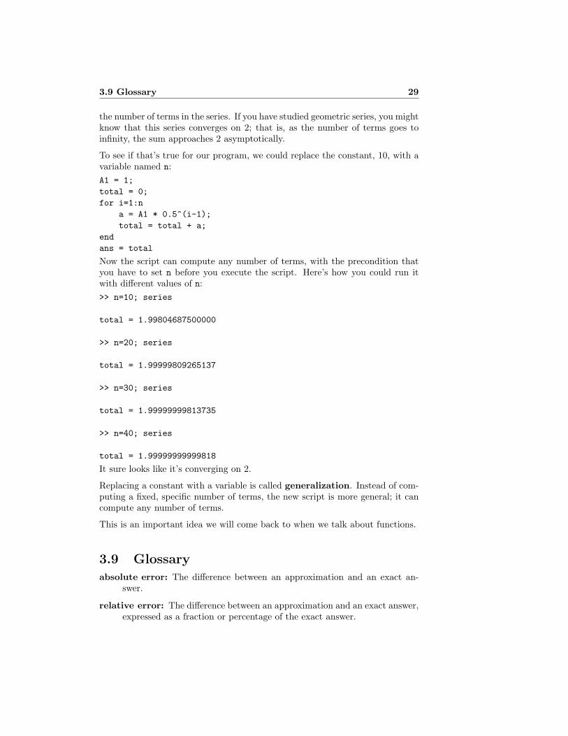
To see if that’s true for our program, we could replace the constant, 10, with avariable named n:
A1 = 1;
total = 0;
for i=1:n
a = A1 * 0.5^(i-1);
total = total + a;
end
ans = total
Now the script can compute any number of terms, with the precondition thatyou have to set n before you execute the script. Here’s how you could run itwith different values of n:
>> n=10; series
total = 1.99804687500000
>> n=20; series
total = 1.99999809265137
>> n=30; series
total = 1.99999999813735
>> n=40; series
total = 1.99999999999818
It sure looks like it’s converging on 2.
Replacing a constant with a variable is called generalization. Instead of com-puting a fixed, specific number of terms, the new script is more general; it cancompute any number of terms.
This is an important idea we will come back to when we talk about functions.
3.9 Glossary
absolute error: The difference between an approximation and an exact an-swer.
relative error: The difference between an approximation and an exact answer,expressed as a fraction or percentage of the exact answer.
30 Loops
loop: A part of a program that runs repeatedly.
loop variable: A variable, defined in a for statement, that gets assigned adifferent value each time through the loop.
range: The set of values assigned to the loop variable, often specified with thecolon operator; for example 1:5.
body: The statements inside the for loop that are run repeatedly.
sequence: In mathematics, a set of numbers that correspond to the positiveintegers.
element: A member of the set of numbers in a sequence.
recurrently: A way of computing the next element of a sequence based onprevious elements.
directly: A way of computing an element in a sequence without using previouselements.
series: The sum of the elements in a sequence.
accumulator: A variable that is used to accumulate a result a little bit at atime.
generalization: A way to make a program more versatile, for example byreplacing a specific value with a variable that can have any value.
3.10 Exercises
Exercise 3.5 We have already seen the Fibonacci sequence, F , which is definedrecurrently as
Fi = Fi−1 + Fi−2
In order to get started, you have to specify the first two elements, but once youhave those, you can compute the rest. The most common Fibonacci sequencestarts with F1 = 1 and F2 = 1.
Write a script called fibonacci2 that uses a for loop to compute the first 10elements of this Fibonacci sequence. As a postcondition, your script shouldassign the 10th element to ans.
Now generalize your script so that it computes the nth element for any valueof n, with the precondition that you have to set n before you run the script. Tokeep things simple for now, you can assume that n is greater than 2.
3.10 Exercises 31
Hint: you will have to use two variables to keep track of the previous two ele-ments of the sequence. You might want to call them prev1 and prev2. Initially,prev1 = F1 and prev2 = F2. At the end of the loop, you will have to updateprev1 and prev2; think carefully about the order of the updates!
Exercise 3.6 Write a script named fib plot that loops i through a rangefrom 1 to 20, uses fibonacci2 to compute Fibonacci numbers, and plots Fi foreach i with a series of red circles.

32 Loops
Chapter 4
Vectors
4.1 Checking preconditions
Some of the loops in the previous chapter don’t work if the value of n isn’t setcorrectly before the loop runs. For example, this loop computes the sum of thefirst n elements of a geometric sequence:
A1 = 1;
total = 0;
for i=1:n
a = A1 * 0.5^(i-1);
total = total + a;
end
ans = total
It works for any positive value of n, but what if n is negative? In that case, youget:
total = 0
Why? Because the expression 1:-1 means “all the numbers from 1 to -1, count-ing up by 1.” It’s not immediately obvious what that should mean, but MAT-LAB’s interpretation is that there aren’t any numbers that fit that description,so the result is
>> 1:-1
ans = Empty matrix: 1-by-0
If the matrix is empty, you might expect it to be “0-by-0,” but there you haveit. In any case, if you loop over an empty range, the loop never runs at all,which is why in this example the value of total is zero for any negative valueof n.
34 Vectors
If you are sure that you will never make a mistake, and that the preconditionsof your functions will always be satisfied, then you don’t have to check. Butfor the rest of us, it is dangerous to write a script, like this one, that quietlyproduces the wrong answer (or at least a meaningless answer) if the input valueis negative. A better alternative is to use an if statement.
4.2 if
The if statement allows you to check for certain conditions and execute state-ments if the conditions are met. In the previous example, we could write:
if n<0
ans = NaN
end
The syntax is similar to a for loop. The first line specifies the condition weare interested in; in this case we are asking if n is negative. If it is, MATLABexecutes the body of the statement, which is the indented sequence of statementsbetween the if and the end.
MATLAB doesn’t require you to indent the body of an if statement, but itmakes your code more readable, so you should do it, and don’t make me tellyou again.
In this example, the “right” thing to do if n is negative is to set ans = NaN,which is a standard way to indicate that the result is undefined (not a number).
If the condition is not satisfied, the statements in the body are not executed.Sometimes there are alternative statements to execute when the condition isfalse. In that case you can extend the if statement with an else clause.
The complete version of the previous example might look like this:
if n<0
ans = NaN
else
A1 = 1;
total = 0;
for i=1:n
a = A1 * 0.5^(i-1);
total = total + a;
end
ans = total
end
Statements like if and for that contain other statements are called compoundstatements. All compound statements end with, well, end.
In this example, one of the statements in the else clause is a for loop. Puttingone compound statement inside another is legal and common, and sometimescalled nesting.
4.3 Relational operators 35
4.3 Relational operators
The operators that compare values, like < and > are called relational operatorsbecause they test the relationship between two values. The result of a relationaloperator is one of the logical values: either 1, which represents “true,” or 0,which represents “false.”
Relational operators often appear in if statements, but you can also evaluatethem at the prompt:
>> x = 5;
>> x < 10
ans = 1
You can assign a logical value to a variable:
>> flag = x > 10
flag = 0
A variable that contains a logical value is often called a flag because it flags thestatus of some condition.
The other relational operators are <= and >=, which are self-explanatory, ==,for “equal,” and ~=, for “not equal.” (In some logic notations, the tilde is thesymbol for “not.”)
Don’t forget that == is the operator that tests equality, and = is the assignmentoperator. If you try to use = in an if statement, you get a syntax error:
if x=5
??? if x=5
|
Error: The expression to the left of the equals sign is not a valid
target for an assignment.
MATLAB thinks you are making an assignment to a variable named if x!
4.4 Logical operators
To test if a number falls in an interval, you might be tempted to write somethinglike 0 < x < 10, but that would be wrong, so very wrong. Unfortunately, inmany cases, you will get the right answer for the wrong reason. For example:
>> x = 5;
>> 0 < x < 10 % right for the wrong reason
ans = 1
But don’t be fooled!
36 Vectors
>> x = 17
>> 0 < x < 10 % just plain wrong
ans = 1
The problem is that MATLAB is evaluating the operators from left to right, sofirst it checks if 0<x. It is, so the result is 1. Then it compares the logical value1 (not the value of x) to 10. Since 1<10, the result is true, even though x is notin the interval.
For beginning programmers, this is an evil, evil bug!
One way around this problem is to use a nested if statement to check the twoconditions separately:
ans = 0
if 0<x
if x<10
ans = 1
end
end
But it is more concise to use the AND operator, &&, to combine the conditions.
>> x = 5;
>> 0<x && x<10
ans = 1
>> x = 17;
>> 0<x && x<10
ans = 0
The result of AND is true if both of the operands are true. The OR operator,||, is true if either or both of the operands are true.
4.5 Vectors
The values we have seen so far are all single numbers, which are called scalarsto contrast them with vectors and matrices, which are collections of numbers.
A vector in MATLAB is similar to a sequence in mathematics; it is a set ofnumbers that correspond to positive integers. What we called a “range” in theprevious chapter was actually a vector.
In general, anything you can do with a scalar, you can also do with a vector.You can assign a vector value to a variable:
4.6 Vector arithmetic 37
>> X = 1:5
X = 1 2 3 4 5
Variables that contain vectors are often capital letters. That’s just a convention;MATLAB doesn’t require it, but for beginning programmers it is a useful wayto remember what is a scalar and what is a vector.
Just as with sequences, the numbers that make up the vector are called ele-ments.
4.6 Vector arithmetic
You can perform arithmetic with vectors, too. If you add a scalar to a vector,MATLAB increments each element of the vector:
>> Y = X+5
Y = 6 7 8 9 10
The result is a new vector; the original value of X is not changed.
If you add two vectors, MATLAB adds the corresponding elements of eachvector and creates a new vector that contains the sums:
>> Z = X+Y
Z = 7 9 11 13 15
But adding vectors only works if the operands are the same size. Otherwise:
>> W = 1:3
W = 1 2 3
>> X+W
??? Error using ==> plus
Matrix dimensions must agree.
The error message in this case is confusing, because we are thinking of thesevalues as vectors, not matrices. The problem is a slight mismatch between mathvocabulary and MATLAB vocabulary.
4.7 Everything is a matrix
In math (specifically in linear algebra) a vector is a one-dimensional sequenceof values and a matrix is two-dimensional (and, if you want to think of it thatway, a scalar is zero-dimensional). In MATLAB, everything is a matrix.
38 Vectors
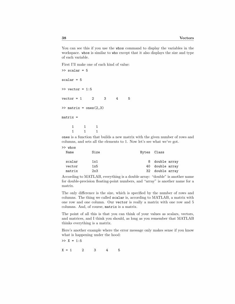
You can see this if you use the whos command to display the variables in theworkspace. whos is similar to who except that it also displays the size and typeof each variable.
First I’ll make one of each kind of value:
>> scalar = 5
scalar = 5
>> vector = 1:5
vector = 1 2 3 4 5
>> matrix = ones(2,3)
matrix =
1 1 1
1 1 1
ones is a function that builds a new matrix with the given number of rows andcolumns, and sets all the elements to 1. Now let’s see what we’ve got.
>> whos
Name Size Bytes Class
scalar 1x1 8 double array
vector 1x5 40 double array
matrix 2x3 32 double array
According to MATLAB, everything is a double array: “double” is another namefor double-precision floating-point numbers, and “array” is another name for amatrix.
The only difference is the size, which is specified by the number of rows andcolumns. The thing we called scalar is, according to MATLAB, a matrix withone row and one column. Our vector is really a matrix with one row and 5columns. And, of course, matrix is a matrix.
The point of all this is that you can think of your values as scalars, vectors,and matrices, and I think you should, as long as you remember that MATLABthinks everything is a matrix.
Here’s another example where the error message only makes sense if you knowwhat is happening under the hood:
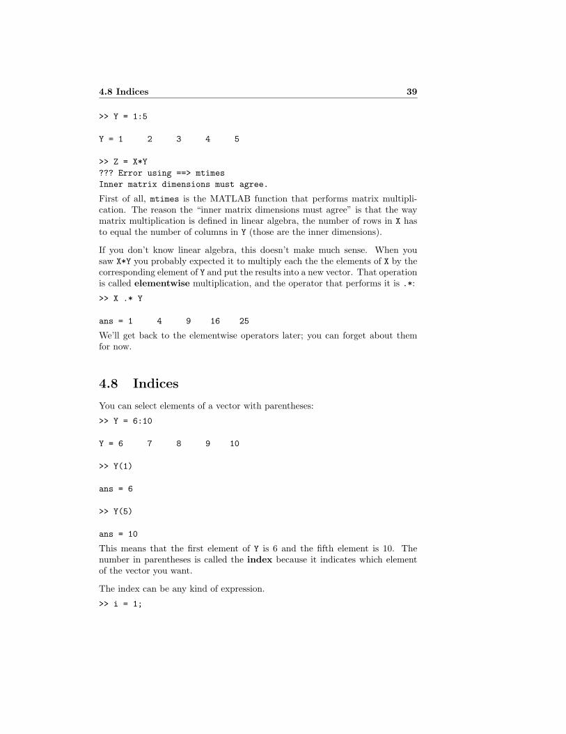
>> X = 1:5
X = 1 2 3 4 5
4.8 Indices 39
>> Y = 1:5
Y = 1 2 3 4 5
>> Z = X*Y
??? Error using ==> mtimes
Inner matrix dimensions must agree.
First of all, mtimes is the MATLAB function that performs matrix multipli-cation. The reason the “inner matrix dimensions must agree” is that the waymatrix multiplication is defined in linear algebra, the number of rows in X hasto equal the number of columns in Y (those are the inner dimensions).
If you don’t know linear algebra, this doesn’t make much sense. When yousaw X*Y you probably expected it to multiply each the the elements of X by thecorresponding element of Y and put the results into a new vector. That operationis called elementwise multiplication, and the operator that performs it is .*:
>> X .* Y
ans = 1 4 9 16 25
We’ll get back to the elementwise operators later; you can forget about themfor now.
4.8 Indices
You can select elements of a vector with parentheses:
>> Y = 6:10
Y = 6 7 8 9 10
>> Y(1)
ans = 6
>> Y(5)
ans = 10
This means that the first element of Y is 6 and the fifth element is 10. Thenumber in parentheses is called the index because it indicates which elementof the vector you want.
The index can be any kind of expression.
>> i = 1;
40 Vectors
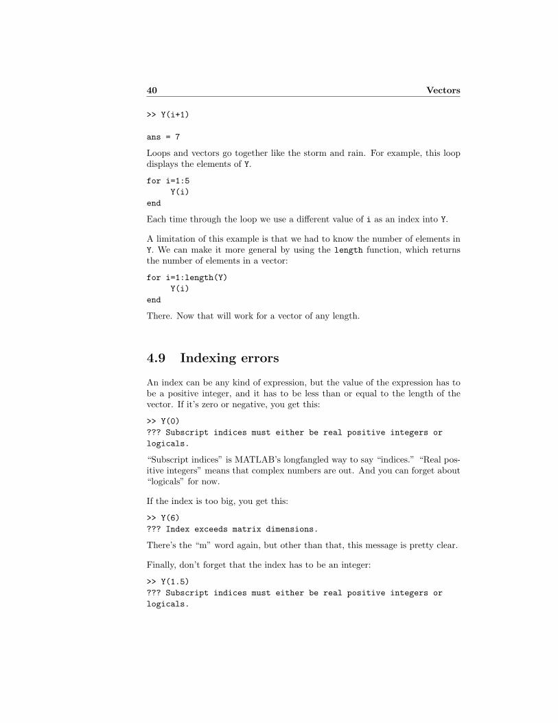
>> Y(i+1)
ans = 7
Loops and vectors go together like the storm and rain. For example, this loopdisplays the elements of Y.
for i=1:5
Y(i)
end
Each time through the loop we use a different value of i as an index into Y.
A limitation of this example is that we had to know the number of elements inY. We can make it more general by using the length function, which returnsthe number of elements in a vector:
for i=1:length(Y)
Y(i)
end
There. Now that will work for a vector of any length.
4.9 Indexing errors
An index can be any kind of expression, but the value of the expression has tobe a positive integer, and it has to be less than or equal to the length of thevector. If it’s zero or negative, you get this:
>> Y(0)
??? Subscript indices must either be real positive integers or
logicals.
“Subscript indices” is MATLAB’s longfangled way to say “indices.” “Real pos-itive integers” means that complex numbers are out. And you can forget about“logicals” for now.
If the index is too big, you get this:
>> Y(6)
??? Index exceeds matrix dimensions.
There’s the “m” word again, but other than that, this message is pretty clear.
Finally, don’t forget that the index has to be an integer:
>> Y(1.5)
??? Subscript indices must either be real positive integers or
logicals.
4.10 Vectors and sequences 41
4.10 Vectors and sequences
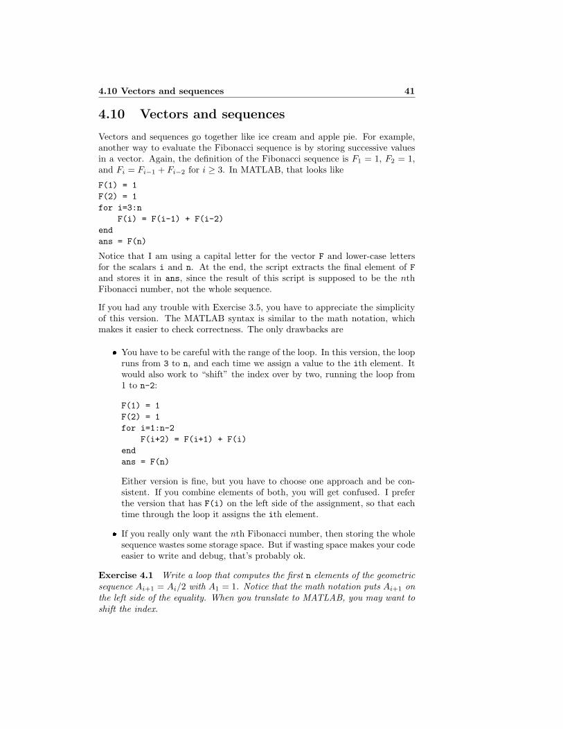
Vectors and sequences go together like ice cream and apple pie. For example,another way to evaluate the Fibonacci sequence is by storing successive valuesin a vector. Again, the definition of the Fibonacci sequence is F1 = 1, F2 = 1,and Fi = Fi−1 + Fi−2 for i ≥ 3. In MATLAB, that looks like
F(1) = 1
F(2) = 1
for i=3:n
F(i) = F(i-1) + F(i-2)
end
ans = F(n)
Notice that I am using a capital letter for the vector F and lower-case lettersfor the scalars i and n. At the end, the script extracts the final element of Fand stores it in ans, since the result of this script is supposed to be the nthFibonacci number, not the whole sequence.
If you had any trouble with Exercise 3.5, you have to appreciate the simplicityof this version. The MATLAB syntax is similar to the math notation, whichmakes it easier to check correctness. The only drawbacks are
� You have to be careful with the range of the loop. In this version, the loopruns from 3 to n, and each time we assign a value to the ith element. Itwould also work to “shift” the index over by two, running the loop from1 to n-2:
F(1) = 1
F(2) = 1
for i=1:n-2
F(i+2) = F(i+1) + F(i)
end
ans = F(n)
Either version is fine, but you have to choose one approach and be con-sistent. If you combine elements of both, you will get confused. I preferthe version that has F(i) on the left side of the assignment, so that eachtime through the loop it assigns the ith element.
� If you really only want the nth Fibonacci number, then storing the wholesequence wastes some storage space. But if wasting space makes your codeeasier to write and debug, that’s probably ok.
Exercise 4.1 Write a loop that computes the first n elements of the geometricsequence Ai+1 = Ai/2 with A1 = 1. Notice that the math notation puts Ai+1 onthe left side of the equality. When you translate to MATLAB, you may want toshift the index.
42 Vectors
4.11 Plotting vectors
Plotting and vectors go together like the moon and June, whatever that means.If you call plot with a single vector as an argument, MATLAB plots the indiceson the x-axis and the elements on the y-axis. To plot the Fibonacci numberswe computed in the previous section:
plot(F)
This display is often useful for debugging, especially if your vectors are bigenough that displaying the elements on the screen is unwieldy.
If you call plot with two vectors as arguments, MATLAB plots the second oneas a function of the first; that is, it treats the first vector as a sequence of xvalues and the second as corresponding y value and plots a sequence of (x, y)points.
X = 1:5
Y = 6:10
plot(X, Y)
By default, MATLAB draws a blue line, but you can override that setting withthe same kind of string we saw in Section 3.5. For example, the string ’ro-’
tells MATLAB to plot a red circle at each data point; the hyphen means thepoints should be connected with a line.
In this example, I stuck with the convention of naming the first argument X
(since it is plotted on the x-axis) and the second Y. There is nothing specialabout these names; you could just as well plot X as a function of Y. MATLABalways treats the first vector as the “independent” variable, and the second asthe “dependent” variable (if those terms are familiar to you).
4.12 Reduce
A frequent use of loops is to run through the elements of an array and add themup, or multiply them together, or compute the sum of their squares, etc. Thiskind of operation is called reduce, because it reduces a vector with multipleelements down to a single scalar.
For example, this loop adds up the elements of a vector named X (which weassume has been defined).
total = 0
for i=1:length(X)
total = total + X(i)
end
ans = total
The use of total as an accumulator is similar to what we saw in Section 3.7.Again, we use the length function to find the upper bound of the range, so this
4.13 Apply 43
loop will work regardless of the length of X. Each time through the loop, we addin the ith element of X, so at the end of the loop total contains the sum of theelements.
Exercise 4.2 Write a similar loop that multiplies all the elements of a vectortogether. You might want to call the accumulator product, and you might wantto think about the initial value you give it before the loop.
4.13 Apply
Another common use of a loop is to run through the elements of a vector,perform some operation on the elements, and create a new vector with theresults. This kind of operation is called apply, because you apply the operationto each element in the vector.
For example, the following loop computes a vector Y that contains the squaresof the elements of X (assuming, again, that X is already defined).
for i=1:length(X)
Y(i) = X(i)^2
end
Exercise 4.3 Write a loop that computes a vector Y that contains the sines ofthe elements of X. To test your loop, write a script that
1. Uses linspace (see the documentation) to assign to X a vector with 100elements running from 0 to 2π.
2. Uses your loop to store the sines in Y.
3. Plots the elements of Y as a function of the elements of X.
4.14 Search
Yet another use of loops is to search the elements of a vector and return the indexof the value you are looking for (or the first value that has a particular property).For example, if a vector contains the computed altitude of a falling object, youmight want to know the index where the object touches down (assuming thatthe ground is at altitude 0).
To create some fake data, we’ll use an extended version of the colon operator:
X = 10:-1:-10
The values in this range run from 10 to -10, with a step size of -1. The stepsize is the interval between elements of the range.
The following loop finds the index of the element 0 in X:
44 Vectors
for i=1:length(X)
if X(i) == 0
ans = i
end
end
One funny thing about this loop is that it keeps going after it finds what it islooking for. That might be what you want; if the target value appears morethan one, this loop provides the index of the last one.
But if you want the index of the first one (or you know that there is only one),you can save some unnecessary looping by using the break statement.
for i=1:length(X)
if X(i) == 0
ans = i
break
end
end
break does pretty much what it sounds like. It ends the loop and proceedsimmediately to the next statement after the loop (in this case, there isn’t one,so the script ends).
This example demonstrates the basic idea of a search, but it also demonstratesa dangerous use of the if statement. Remember that floating-point values areoften only approximately right. That means that if you look for a perfect match,you might not find it. For example, try this:
X = linspace(1,2)
for i=1:length(X)
Y(i) = sin(X(i))
end
plot(X, Y)
You can see in the plot that the value of sinx goes through 0.9 in this range,but if you search for the index where Y(i) == 0.9, you will come up empty.
for i=1:length(Y)
if Y(i) == 0.9
ans = i
break
end
end
The condition is never true, so the body of the if statement is never executed.
Even though the plot shows a continuous line, don’t forget that X and Y aresequences of discrete (and usually approximate) values. As a rule, you should(almost) never use the == operator to compare floating-point values. There area number of ways to get around this limitation; we will get to them later.
4.15 Spoiling the fun 45
Exercise 4.4 Write a loop that finds the index of the first negative number ina vector and stores it in ans. If there are no negative numbers, it should setans to -1 (which is not a legal index, so it is a good way to indicate the specialcase).
4.15 Spoiling the fun
Experienced MATLAB programmers would never write the kind of loops in thischapter, because MATLAB provides simpler and faster ways to perform manyreduce, filter and search operations.
For example, the sum function computes the sum of the elements in a vectorand prod computes the product.
Many apply operations can be done with elementwise operators. The followingstatement is more concise than the loop in Section 4.13
Y = X .^ 2
Also, most built-in MATLAB functions work with vectors:
X = linspace(0, 2*pi)
Y = sin(X)
plot(X, Y)
Finally, the find function can perform search operations, but understanding itrequires a couple of concepts we haven’t got to, so for now you are better off onyour own.
I started with simple loops because I wanted to demonstrate the basic conceptsand give you a chance to practice. At some point you will probably have towrite a loop for which there is no MATLAB shortcut, but you have to workyour way up from somewhere.
If you understand loops and you are are comfortable with the shortcuts, feelfree to use them! Otherwise, you can always write out the loop.
Exercise 4.5 Write an expression that computes the sum of the squares of theelements of a vector.
4.16 Glossary
compound: A statement, like if and for, that contains other statements inan indented body.
nesting: Putting one compound statement in the body of another.
relational operator: An operator that compares two values and generates alogical value as a result.
46 Vectors
logical value: A value that represents either “true” or “false”. MATLAB usesthe values 1 and 0, respectively.
flag: A variable that contains a logical value, often used to store the status ofsome condition.
scalar: A single value.
vector: A sequence of values.
matrix: A two-dimensional collection of values (also called “array” in someMATLAB documentation).
index: An integer value used to indicate one of the values in a vector or matrix(also called subscript in some MATLAB documentation).
element: One of the values in a vector or matrix.
elementwise: An operation that acts on the individual elements of a vector ormatrix (unlike some linear algebra operations).
reduce: A way of processing the elements of a vector and generating a singlevalue; for example, the sum of the elements.
apply: A way of processing a vector by performing some operation on each ofthe elements, producing a vector that contains the results.
search: A way of processing a vector by examining the elements in order untilone is found that has the desired property.
4.17 Exercises
Exercise 4.6 The ratio of consecutive Fibonacci numbers, Fn+1/Fn, convergesto a constant value as n increases. Write a script that computes a vector withthe first n elements of a Fibonacci sequence (assuming that the variable n isdefined), and then computes a new vector that contains the ratios of consecutiveFibonacci numbers. Plot this vector to see if it seems to converge. What valuedoes it converge on?
Exercise 4.7 A certain famous system of differential equations can be approx-imated by a system of difference equations that looks like this:
xi+1 = xi + σ (yi − xi) dt (4.1)
yi+1 = yi + [xi(r − zi)− yi] dt (4.2)
zi+1 = zi + (xiyi − bzi) dt (4.3)
4.17 Exercises 47
� Write a script that computes the first 10 elements of the sequences X, Yand Z and stores them in vectors named X, Y and Z.
Use the initial values X1 = 1, Y1 = 2 and Z1 = 3, with values σ = 10,b = 8/3 and r = 28, and with time step dt = 0.01.
� Read the documentation for plot3 and comet3 and plot the results in 3dimensions.
� Once the code is working, use semi-colons to suppress the output and thenrun the program with sequence length 100, 1000 and 10000.
� Run the program again with different starting conditions. What effect doesit have on the result?
� Run the program with different values for σ, b and r and see if you canget a sense of how each variable affects the system.
Exercise 4.8 The logistic map is often cited as an example of how complex,chaotic behaviour can arise from simple non-linear dynamical equations [someof this description is adapted from the Wikipedia page on the logistic map]. Itwas popularized in a seminal 1976 paper by the biologist Robert May.
It has been used to model the biomass of a species in the presence of limitingfactors such as food supply and disease. In this case, there are two processes atwork: (1) A reproductive process increases the biomass of the species in propor-tion to the current population. (2) A starvation process causes the biomass todecrease at a rate proportional to the carrying capacity of the environment lessthe current population.
Mathematically this can be written as
Xi+1 = rXi(1−Xi)
where Xi is a number between zero and one that represents the biomass at yeari, and r is a positive number that represents a combined rate for reproductionand starvation.
� Write a script named logmap that computes the first 50 elements of Xwith r=3.9 and X1=0.5, where r is the parameter of the logistic map andX1 is the initial population.
� Plot the results for a range of values of r from 2.4 to 4.0. How does thebehavior of the system change as you vary r.
� One way to characterize the effect of r is to make a plot with r on thex-axis and biomass on the y axis, and to show, for each value of r, thevalues of biomass that occur in steady state. See if you can figure out howto generate this plot.

48 Vectors
Chapter 5
Functions
5.1 Name Collisions
Remember that all of your scripts run in the same workspace, so if one scriptchanges the value of a variable, all your other scripts see the change. Witha small number of simple scripts, that’s not a problem, but eventually theinteractions between scripts become unmanageable.
For example, the following (increasingly familiar) script computes the sum ofthe first n terms in a geometric sequence, but it also has the side-effect ofassigning values to A1, total, i and a.
A1 = 1;
total = 0;
for i=1:10
a = A1 * 0.5^(i-1);
total = total + a;
end
ans = total
If you were using any of those variable names before calling this script, you mightbe surprised to find, after running the script, that their values had changed. Ifyou have two scripts that use the same variable names, you might find that theywork separately and then break when you try to combine them. This kind ofinteraction is called a name collision.
As the number of scripts you write increases, and they get longer and morecomplex, name collisions become more of a problem. Avoiding this problem isone of the motivations for functions.
50 Functions
5.2 Functions
A function is like a script, except
� Each function has its own workspace, so any variables defined inside afunction only exist while the function is running, and don’t interfere withvariables in other workspaces, even if they have the same name.
� Function inputs and outputs are defined carefully to avoid unexpectedinteractions.
To define a new function, you create an M-file with the name you want, andput a function definition in it. For example, to create a function named myfunc,create an M-file named myfunc.m and put the following definition into it.
function res = myfunc(x)
s = sin(x)
c = cos(x)
res = abs(s) + abs(c)
end
The first word of the file has to be the word function, because that’s howMATLAB tells the difference between a script and a function file.
A function definition is a compound statement. The first line is called thesignature of the function; it defines the inputs and outputs of the function.In this case the input variable is named x. When this function is called, theargument provided by the user will be assigned to x.
The output variable is named res, which is short for “result.” You can callthe output variable whatever you want, but as a convention, I like to call it res.Usually the last thing a function does is assign a value to the output variable.
Once you have defined a new function, you call it the same way you call built-inMATLAB functions. If you call the function as a statement, MATLAB puts theresult into ans:
>> myfunc(1)
s = 0.84147098480790
c = 0.54030230586814
res = 1.38177329067604
ans = 1.38177329067604
But it is more common (and better style) to assign the result to a variable:
>> y = myfunc(1)
5.3 Documentation 51
s = 0.84147098480790
c = 0.54030230586814
res = 1.38177329067604
y = 1.38177329067604
While you are debugging a new function, you might want to display intermediateresults like this, but once it is working, you will want to add semi-colons to makeit a silent function. Most built-in functions are silent; they compute a result,but they don’t display anything (except sometimes warning messages).
Each function has its own workspace, which is created when the function startsand destroyed when the function ends. If you try to access (read or write) thevariables defined inside a function, you will find that they don’t exist.
>> clear
>> y = myfunc(1);
>> who
Your variables are: y
>> s
??? Undefined function or variable 's'.
The only value from the function that you can access is the result, which in thiscase is assigned to y.
If you have variables named s or c in your workspace before you call myfunc,they will still be there when the function completes.
>> s = 1;
>> c = 1;
>> y = myfunc(1);
>> s, c
s = 1
c = 1
So inside a function you can use whatever variable names you want withoutworrying about collisions.
5.3 Documentation
At the beginning of every function file, you should include a comment thatexplains what the function does.
52 Functions
% res = myfunc (x)
% Compute the Manhattan distance from the origin to the
% point on the unit circle with angle (x) in radians.
function res = myfunc (x)
s = sin(x);
c = cos(x);
res = abs(s) + abs(c);
end
When you ask for help, MATLAB prints the comment you provide.
>> help myfunc
res = myfunc (x)
Compute the Manhattan distance from the origin to the
point on the unit circle with angle (x) in radians.
There are lots of conventions about what should be included in these comments.Among other things, it is a good idea to include
� The signature of the function, which includes the name of the function,the input variable(s) and the output variable(s).
� A clear, concise, abstract description of what the function does. An ab-stract description is one that leaves out the details of how the functionworks, and includes only information that someone using the functionneeds to know. You can put additional comments inside the function thatexplain the details.
� An explanation of what the input variables mean; for example, in this caseit is important to note that x is considered to be an angle in radians.
� Any preconditions and postconditions.
5.4 Function names
There are three “gotchas” that come up when you start naming functions. Thefirst is that the “real” name of your function is determined by the file name,not by the name you put in the function signature. As a matter of style, youshould make sure that they are always the same, but if you make a mistake, orif you change the name of a function, it is easy to get confused.
In the spirit of making errors on purpose, change the name of the function inmyfunc to something else, and then run it again.
If this is what you put in myfunc.m:
5.5 Multiple input variables 53
function res = something_else (x)
s = sin(x);
c = cos(x);
res = abs(s) + abs(c);
end
Then here’s what you’ll get:
>> y = myfunc(1);
>> y = something_else(1);
??? Undefined command/function 'something_else'.
The second gotcha is that the name of the file can’t have spaces. For example,if you write a function and name the file my func.m, which the MATLAB editorwill happily allow you to do, and then try to run it, you get:
>> y = my func(1)
??? y = my func(1)
|
Error: Unexpected MATLAB expression.
The third gotcha is that your function names can collide with built-in MATLABfunctions. For example, if you create an M-file named sum.m, and then call sum,MATLAB might call your new function, not the built-in version! Which oneactually gets called depends on the order of the directories in the search path,and (in some cases) on the arguments. As an example, put the following codein a file named sum.m:
function res = sum(x)
res = 7;
end
And then try this:
>> sum(1:3)
ans = 6
>> sum
ans = 7
In the first case MATLAB used the built-in function; in the second case it ranyour function! This kind of interaction can be very confusing. Before you createa new function, check to see if there is already a MATLAB function with thesame name. If there is, choose another name!
5.5 Multiple input variables
Functions can, and often do, take more than one input variable. For example,the following function takes two input variables, a and b:

54 Functions
function res = hypotenuse(a, b)
res = sqrt(a^2 + b^2);
end
If you remember the Pythagorean Theorem, you probably figured out that thisfunction computes the length of the hypotenuse of a right triangle if the lengthsof the adjacent sides are a and b. (There is a MATLAB function called hypot
that does the same thing.)
If we call it from the Command Window with arguments 3 and 4, we can confirmthat the length of the third side is 5.
>> c = hypotenuse(3, 4)
c = 5
The arguments you provide are assigned to the input variables in order, so inthis case 3 is assigned to a and 4 is assigned to b. MATLAB checks that youprovide the right number of arguments; if you provide too few, you get
>> c = hypotenuse(3)
??? Input argument "b" is undefined.
Error in ==> hypotenuse at 2
res = sqrt(a^2 + b^2);
This error message is confusing, because it suggests that the problem is inhypotenuse rather than in the function call. Keep that in mind when you aredebugging.
If you provide too many arguments, you get
>> c = hypotenuse(3, 4, 5)
??? Error using ==> hypotenuse
Too many input arguments.
Which is a better message.
5.6 Logical functions
In Section 4.4 we used logical operators to compare values. MATLAB alsoprovides logical functions that check for certain conditions and return logicalvalues: 1 for “true” and 0 for “false”.
For example, isprime checks to see whether a number is prime.
>> isprime(17)
ans = 1
>> isprime(21)
ans = 0
5.7 An incremental development example 55
The functions isscalar and isvector check whether a value is a scalar orvector; if both are false, you can assume it is a matrix (at least for now).
To check whether a value you have computed is an integer, you might be temptedto use isinteger. But that would be wrong, so very wrong. isinteger checkswhether a value belongs to one of the integer types (a topic we have not dis-cussed); it doesn’t check whether a floating-point value happens to be integral.
>> c = hypotenuse(3, 4)
c = 5
>> isinteger(c)
ans = 0
To do that, we have to write our own logical function, which we’ll callisintegral:
function res = isintegral(x)
if round(x) == x
res = 1;
else
res = 0;
end
end
This function is good enough for most applications, but remember that floating-point values are only approximately right; in some cases the approximation isan integer but the actual value is not.
5.7 An incremental development example
Let’s say that we want to write a program to search for “Pythagorean triples:”sets of integral values, like 3, 4 and 5, that are the lengths of the sides of a righttriangle. In other words, we would like to find integral values a, b and c suchthat a2 + b2 = c2.
Here are the steps we will follow to develop the program incrementally.
� Write a script named find triples and start with a simple statementlike x=5.
� Write a loop that enumerates values of a from 1 to 3, and displays them.
� Write a nested loop that enumerates values of b from 1 to 4, and displaysthem.
� Inside the loop, call hypotenuse to compute c and display it.
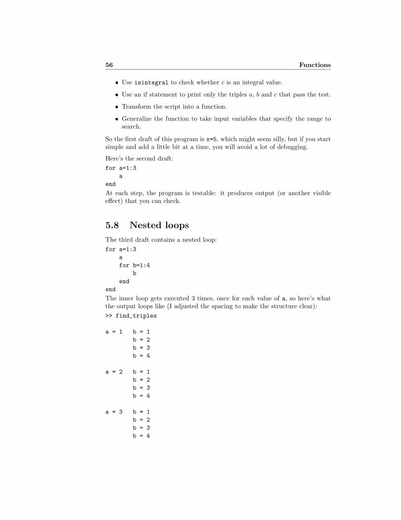
56 Functions
� Use isintegral to check whether c is an integral value.
� Use an if statement to print only the triples a, b and c that pass the test.
� Transform the script into a function.
� Generalize the function to take input variables that specify the range tosearch.
So the first draft of this program is x=5, which might seem silly, but if you startsimple and add a little bit at a time, you will avoid a lot of debugging.
Here’s the second draft:
for a=1:3
a
end
At each step, the program is testable: it produces output (or another visibleeffect) that you can check.
5.8 Nested loops
The third draft contains a nested loop:
for a=1:3
a
for b=1:4
b
end
end
The inner loop gets executed 3 times, once for each value of a, so here’s whatthe output loops like (I adjusted the spacing to make the structure clear):
>> find_triples
a = 1 b = 1
b = 2
b = 3
b = 4
a = 2 b = 1
b = 2
b = 3
b = 4
a = 3 b = 1
b = 2
b = 3
b = 4
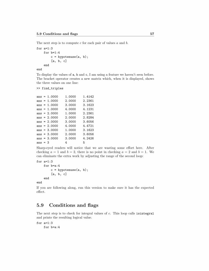
5.9 Conditions and flags 57
The next step is to compute c for each pair of values a and b.
for a=1:3
for b=1:4
c = hypotenuse(a, b);
[a, b, c]
end
end
To display the values of a, b and c, I am using a feature we haven’t seen before.The bracket operator creates a new matrix which, when it is displayed, showsthe three values on one line:
>> find_triples
ans = 1.0000 1.0000 1.4142
ans = 1.0000 2.0000 2.2361
ans = 1.0000 3.0000 3.1623
ans = 1.0000 4.0000 4.1231
ans = 2.0000 1.0000 2.2361
ans = 2.0000 2.0000 2.8284
ans = 2.0000 3.0000 3.6056
ans = 2.0000 4.0000 4.4721
ans = 3.0000 1.0000 3.1623
ans = 3.0000 2.0000 3.6056
ans = 3.0000 3.0000 4.2426
ans = 3 4 5
Sharp-eyed readers will notice that we are wasting some effort here. Afterchecking a = 1 and b = 2, there is no point in checking a = 2 and b = 1. Wecan eliminate the extra work by adjusting the range of the second loop:
for a=1:3
for b=a:4
c = hypotenuse(a, b);
[a, b, c]
end
end
If you are following along, run this version to make sure it has the expectedeffect.
5.9 Conditions and flags
The next step is to check for integral values of c. This loop calls isintegraland prints the resulting logical value.
for a=1:3
for b=a:4
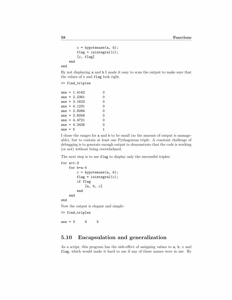
58 Functions
c = hypotenuse(a, b);
flag = isintegral(c);
[c, flag]
end
end
By not displaying a and b I made it easy to scan the output to make sure thatthe values of c and flag look right.
>> find_triples
ans = 1.4142 0
ans = 2.2361 0
ans = 3.1623 0
ans = 4.1231 0
ans = 2.8284 0
ans = 3.6056 0
ans = 4.4721 0
ans = 4.2426 0
ans = 5 1
I chose the ranges for a and b to be small (so the amount of output is manage-able), but to contain at least one Pythagorean triple. A constant challenge ofdebugging is to generate enough output to demonstrate that the code is working(or not) without being overwhelmed.
The next step is to use flag to display only the successful triples:
for a=1:3
for b=a:4
c = hypotenuse(a, b);
flag = isintegral(c);
if flag
[a, b, c]
end
end
end
Now the output is elegant and simple:
>> find_triples
ans = 3 4 5
5.10 Encapsulation and generalization
As a script, this program has the side-effect of assigning values to a, b, c andflag, which would make it hard to use if any of those names were in use. By
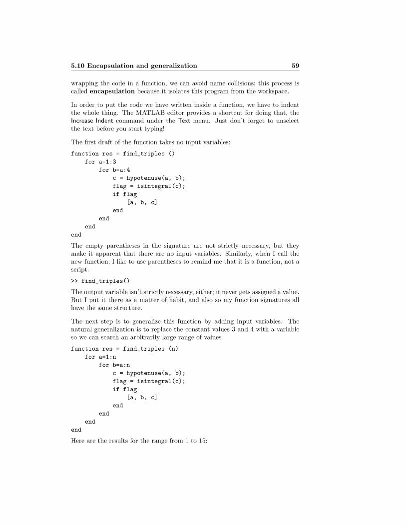
5.10 Encapsulation and generalization 59
wrapping the code in a function, we can avoid name collisions; this process iscalled encapsulation because it isolates this program from the workspace.
In order to put the code we have written inside a function, we have to indentthe whole thing. The MATLAB editor provides a shortcut for doing that, theIncrease Indent command under the Text menu. Just don’t forget to unselectthe text before you start typing!
The first draft of the function takes no input variables:
function res = find_triples ()
for a=1:3
for b=a:4
c = hypotenuse(a, b);
flag = isintegral(c);
if flag
[a, b, c]
end
end
end
end
The empty parentheses in the signature are not strictly necessary, but theymake it apparent that there are no input variables. Similarly, when I call thenew function, I like to use parentheses to remind me that it is a function, not ascript:
>> find_triples()
The output variable isn’t strictly necessary, either; it never gets assigned a value.But I put it there as a matter of habit, and also so my function signatures allhave the same structure.
The next step is to generalize this function by adding input variables. Thenatural generalization is to replace the constant values 3 and 4 with a variableso we can search an arbitrarily large range of values.
function res = find_triples (n)
for a=1:n
for b=a:n
c = hypotenuse(a, b);
flag = isintegral(c);
if flag
[a, b, c]
end
end
end
end
Here are the results for the range from 1 to 15:
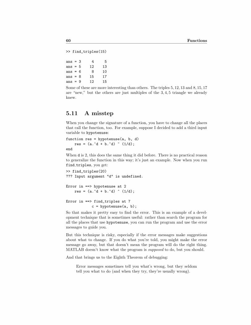
60 Functions
>> find_triples(15)
ans = 3 4 5
ans = 5 12 13
ans = 6 8 10
ans = 8 15 17
ans = 9 12 15
Some of these are more interesting than others. The triples 5, 12, 13 and 8, 15, 17are “new,” but the others are just multiples of the 3, 4, 5 triangle we alreadyknew.
5.11 A misstep
When you change the signature of a function, you have to change all the placesthat call the function, too. For example, suppose I decided to add a third inputvariable to hypotenuse:
function res = hypotenuse(a, b, d)
res = (a.^d + b.^d) ^ (1/d);
end
When d is 2, this does the same thing it did before. There is no practical reasonto generalize the function in this way; it’s just an example. Now when you runfind triples, you get:
>> find_triples(20)
??? Input argument "d" is undefined.
Error in ==> hypotenuse at 2
res = (a.^d + b.^d) ^ (1/d);
Error in ==> find_triples at 7
c = hypotenuse(a, b);
So that makes it pretty easy to find the error. This is an example of a devel-opment technique that is sometimes useful: rather than search the program forall the places that use hypotenuse, you can run the program and use the errormessages to guide you.
But this technique is risky, especially if the error messages make suggestionsabout what to change. If you do what you’re told, you might make the errormessage go away, but that doesn’t mean the program will do the right thing.MATLAB doesn’t know what the program is supposed to do, but you should.
And that brings us to the Eighth Theorem of debugging:
Error messages sometimes tell you what’s wrong, but they seldomtell you what to do (and when they try, they’re usually wrong).
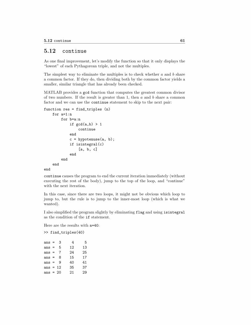
5.12 continue 61
5.12 continue
As one final improvement, let’s modify the function so that it only displays the“lowest” of each Pythagorean triple, and not the multiples.
The simplest way to eliminate the multiples is to check whether a and b sharea common factor. If they do, then dividing both by the common factor yields asmaller, similar triangle that has already been checked.
MATLAB provides a gcd function that computes the greatest common divisorof two numbers. If the result is greater than 1, then a and b share a commonfactor and we can use the continue statement to skip to the next pair:
function res = find_triples (n)
for a=1:n
for b=a:n
if gcd(a,b) > 1
continue
end
c = hypotenuse(a, b);
if isintegral(c)
[a, b, c]
end
end
end
end
continue causes the program to end the current iteration immediately (withoutexecuting the rest of the body), jump to the top of the loop, and “continue”with the next iteration.
In this case, since there are two loops, it might not be obvious which loop tojump to, but the rule is to jump to the inner-most loop (which is what wewanted).
I also simplified the program slightly by eliminating flag and using isintegralas the condition of the if statement.
Here are the results with n=40:
>> find_triples(40)
ans = 3 4 5
ans = 5 12 13
ans = 7 24 25
ans = 8 15 17
ans = 9 40 41
ans = 12 35 37
ans = 20 21 29
62 Functions
There is an interesting connection between Fibonacci numbers and Pythagoreantriples. If F is a Fibonacci sequence, then
(FnFn+3, 2Fn+1Fn+2, F2n+1 + F 2
n+2)
is a Pythagorean triple for all n ≥ 1.
Exercise 5.1 Write a function named fib triple that takes an input vari-able n, uses fibonacci2 to compute the first n Fibonacci numbers, and thenchecks whether this formula produces a Pythagorean triple for each number inthe sequence.
5.13 Mechanism and leap of faith
Let’s review the sequence of steps that occur when you call a function:
1. Before the function starts running, MATLAB creates a new workspace forit.
2. MATLAB evaluates each of the arguments and assigns the resulting values,in order, to the input variables (which live in the new workspace).
3. The body of the code executes. Somewhere in the body (often the lastline) a value gets assigned to the output variable.
4. The function’s workspace is destroyed; the only thing that remains is thevalue of the output variable and any side effects the function had (likedisplaying values or creating a figure).
5. The program resumes from where it left off. The value of the function callis the value of the output variable.
When you are reading a program and you come to a function call, there are twoways to interpret it:
� You can think about the mechanism I just described, and follow the exe-cution of the program into the function and back, or
� You can take the “leap of faith”: assume that the function works correctly,and go on to the next statement after the function call.
When you use built-in functions, it is natural to take the leap of faith, in partbecause you expect that most MATLAB functions work, and in part becauseyou don’t generally have access to the code in the body of the function.
But when you start writing your own functions, you will probably find yourselffollowing the “flow of execution.” This can be useful while you are learning,
5.14 Glossary 63
but as you gain experience, you should get more comfortable with the idea ofwriting a function, testing it to make sure it works, and then forgetting aboutthe details of how it works.
Forgetting about details is called abstraction; in the context of functions,abstraction means forgetting about how a function works, and just assuming(after appropriate testing) that it works.
5.14 Glossary
side-effect: An effect, like modifying the workspace, that is not the primarypurpose of a script.
name collision: The scenario where two scripts that use the same variablename interfere with each other.
input variable: A variable in a function that gets its value, when the functionis called, from one of the arguments.
output variable: A variable in a function that is used to return a value fromthe function to the caller.
signature: The first line of a function definition, which specifies the names ofthe function, the input variables and the output variables.
silent function: A function that doesn’t display anything or generate a figure,or have any other side-effects.
logical function: A function that returns a logical value (1 for “true” or 0 for“false”).
encapsulation: The process of wrapping part of a program in a function inorder to limit interactions (including name collisions) between the functionand the rest of the program.
generalization: Making a function more versatile by replacing specific valueswith input variables.
abstraction: The process of ignoring the details of how a function works inorder to focus on a simpler model of what the function does.
5.15 Exercises
Exercise 5.2 Take any of the scripts you have written so far, encapsulate thecode in an appropriately-named function, and generalize the function by addingone or more input variables.
Make the function silent and then call it from the Command Window and con-firm that you can display the output value.

64 Functions
Chapter 6
Zero-finding
6.1 Why functions?
The previous chapter explained some of the benefits of functions, including
� Each function has its own workspace, so using functions helps avoid namecollisions.
� Functions lend themselves to incremental development: you can debug thebody of the function first (as a script), then encapsulate it as a function,and then generalize it by adding input variables.
� Functions allow you to divide a large problem into small pieces, work onthe pieces one at a time, and then assemble a complete solution.
� Once you have a function working, you can forget about the details of howit works and concentrate on what it does. This process of abstraction isan important tool for managing the complexity of large programs.
Another reason you should consider using functions is that many of the toolsprovided by MATLAB require you to write functions. For example, in thischapter we will use fzero to find solutions of nonlinear equations. Later we willuse ode45 to approximate solutions to differential equations.
6.2 Maps
In mathematics, a map is a correspondence between one set called the rangeand another set called the domain. For each element of the range, the mapspecifies the corresponding element of the domain.
66 Zero-finding
You can think of a sequence as a map from positive integers to elements. Youcan think of a vector as a map from indices to elements. In these cases the mapsare discrete because the elements of the range are countable.
You can also think of a function as a map from inputs to outputs, but in thiscase the range is continuous because the inputs can take any value, not justintegers. (Strictly speaking, the set of floating-point numbers is discrete, butsince floating-point numbers are meant to represent real numbers, we think ofthem as continuous.)
6.3 A note on notation
In this chapter I need to start talking about mathematical functions, and I amgoing to use a notation you might not have seen before.
If you have studied functions in a math class, you have probably seen somethinglike
f(x) = x2 − 2x− 3
which is supposed to mean that f is a function that maps from x to x2−2x−3.The problem is that f(x) is also used to mean the value of f that correspondsto a particular value of x. So I don’t like this notation. I prefer
f : x → x2 − 2x− 3
which means “f is the function that maps from x to x2− 2x− 3.” In MATLAB,this would be expressed like this:
function res = error_func(x)
res = x^2 - 2*x -3;
end
I’ll explain soon why this function is called error func. Now, back to ourregularly-scheduled programming.
6.4 Nonlinear equations
What does it mean to “solve” an equation? That may seem like an obviousquestion, but I want to take a minute to think about it, starting with a simpleexample: let’s say that we want to know the value of a variable, x, but all weknow about it is the relationship x2 = a.
If you have taken algebra, you probably know how to “solve” this equation: youtake the square root of both sides and get x =
√a. Then, with the satisfaction
of a job well done, you move on to the next problem.
6.4 Nonlinear equations 67
But what have you really done? The relationship you derived is equivalent tothe relationship you started with—they contain the same information aboutx—so why is the second one preferable to the first?
There are two reasons. One is that the relationship is now “explicit in x;”because x is all alone on the left side, we can treat the right side as a recipe forcomputing x, assuming that we know the value of a.
The other reason is that the recipe is written in terms of operations we knowhow to perform. Assuming that we know how to compute square roots, we cancompute the value of x for any value of a.
When people talk about solving an equation, what they usually mean is some-thing like “finding an equivalent relationship that is explicit in one of the vari-ables.” In the context of this book, that’s what I will call an analytic solution,to distinguish it from a numerical solution, which is what we are going to donext.
To demonstrate a numerical solution, consider the equation x2 − 2x = 3. Youcould solve this analytically, either by factoring it or by using the quadraticequation, and you would discover that there are two solutions, x = 3 and x =−1. Alternatively, you could solve it numerically by rewriting it as x =
√2x+ 3.
This equation is not explicit, since x appears on both sides, so it is not clearthat this move did any good at all. But suppose that we had some reason toexpect there to be a solution near 4. We could start with x = 4 as an “initialguess,” and then use the equation x =
√2x+ 3 iteratively to compute successive
approximations of the solution.
Here’s what would happen:
>> x = 4;
>> x = sqrt(2*x+3)
x = 3.3166
>> x = sqrt(2*x+3)
x = 3.1037
>> x = sqrt(2*x+3)
x = 3.0344
>> x = sqrt(2*x+3)
x = 3.0114
68 Zero-finding
>> x = sqrt(2*x+3)
x = 3.0038
After each iteration, x is closer to the correct answer, and after 5 iterations, therelative error is about 0.1%, which is good enough for most purposes.
Techniques that generate numerical solutions are called numerical methods.The nice thing about the method I just demonstrated is that it is simple, butit doesn’t always work as well as it did in this example, and it is not used veryoften in practice. We’ll see one of the more practical alternatives in a minute.
6.5 Zero-finding
A nonlinear equation like x2 − 2x = 3 is a statement of equality that is true forsome values of x and false for others. A value that makes it true is a solution;any other value is a non-solution. But for any given non-solution, there is nosense of whether it is close or far from a solution, or where we might look tofind one.
To address this limitation, it is useful to rewrite non-linear equations as zero-finding problems:
� The first step is to define an “error function” that computes how far agiven value of x is from being a solution.
In this example, the error function is
f : x → x2 − 2x− 3
Any value of x that makes f(x) = 0 is also a solution of the originalequation.
� The next step is to find values of x that make f(x) = 0. These values arecalled zeros of the function, or sometimes roots.
Zero-finding lends itself to numerical solution because we can use the values off , evaluated at various values of x, to make reasonable inferences about whereto look for zeros.
For example, if we can find two values x1 and x2 such that f(x1) > 0 andf(x2) < 0, then we can be certain that there is at least one zero between x1
and x2 (provided that we know that f is continuous). In this case we would saythat x1 and x2 bracket a zero.
Here’s what this scenario might look like on a graph:
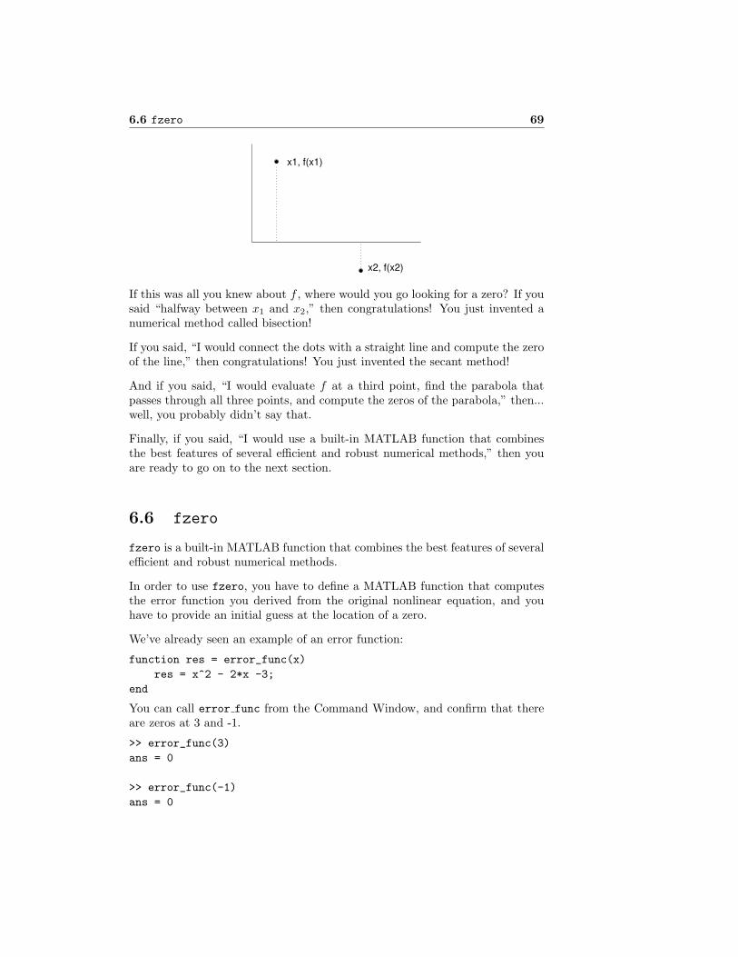
6.6 fzero 69
x1, f(x1)
x2, f(x2)
If this was all you knew about f , where would you go looking for a zero? If yousaid “halfway between x1 and x2,” then congratulations! You just invented anumerical method called bisection!
If you said, “I would connect the dots with a straight line and compute the zeroof the line,” then congratulations! You just invented the secant method!
And if you said, “I would evaluate f at a third point, find the parabola thatpasses through all three points, and compute the zeros of the parabola,” then...well, you probably didn’t say that.
Finally, if you said, “I would use a built-in MATLAB function that combinesthe best features of several efficient and robust numerical methods,” then youare ready to go on to the next section.
6.6 fzero
fzero is a built-in MATLAB function that combines the best features of severalefficient and robust numerical methods.
In order to use fzero, you have to define a MATLAB function that computesthe error function you derived from the original nonlinear equation, and youhave to provide an initial guess at the location of a zero.
We’ve already seen an example of an error function:
function res = error_func(x)
res = x^2 - 2*x -3;
end
You can call error func from the Command Window, and confirm that thereare zeros at 3 and -1.
>> error_func(3)
ans = 0
>> error_func(-1)
ans = 0
70 Zero-finding
But let’s pretend that we don’t know exactly where the roots are; we only knowthat one of them is near 4. Then we could call fzero like this:
>> fzero(@error_func, 4)
ans = 3.0000
Success! We found one of the zeros.
The first argument is a function handle that names the M-file that evaluatesthe error function. The @ symbol allows us to name the function without callingit. The interesting thing here is that you are not actually calling error func
directly; you are just telling fzero where it is. In turn, fzero calls your errorfunction—more than once, in fact.
The second argument is the initial guess. If we provide a different initial guess,we get a different root (at least sometimes).
>> fzero(@error_func, -2)
ans = -1
Alternatively, if you know two values that bracket the root, you can provideboth:
>> fzero(@error_func, [2,4])
ans = 3
The second argument here is actually a vector that contains two elements. Thebracket operator is a convenient way (one of several) to create a new vector.
You might be curious to know how many times fzero calls your function, andwhere. If you modify error func so that it displays the value of x every timeit is called and then run fzero again, you get:
>> fzero(@error_func, [2,4])
x = 2
x = 4
x = 2.75000000000000
x = 3.03708133971292
x = 2.99755211623500
x = 2.99997750209270
x = 3.00000000025200
x = 3.00000000000000
x = 3
x = 3
ans = 3
Not surprisingly, it starts by computing f(2) and f(4). After each iteration,the interval that brackets the root gets smaller; fzero stops when the intervalis so small that the estimated zero is correct to 16 digits. If you don’t need thatmuch precision, you can tell fzero to give you a quicker, dirtier answer (see thedocumentation for details).
6.7 What could go wrong? 71
6.7 What could go wrong?
The most common problem people have with fzero is leaving out the @. In thatcase, you get something like:
>> fzero(error_func, [2,4])
??? Input argument "x" is undefined.
Error in ==> error_func at 2
x
Which is a very confusing error message. The problem is that MATLAB treatsthe first argument as a function call, so it calls error func with no arguments.Since error func requires one argument, the message indicates that the inputargument is “undefined,” although it might be clearer to say that you haven’tprovided a value for it.
Another common problem is writing an error function that never assigns a valueto the output variable. In general, functions should always assign a value to theoutput variable, but MATLAB doesn’t enforce this rule, so it is easy to forget.For example, if you write:
function res = error_func(x)
y = x^2 - 2*x -3
end
and then call it from the Command Window:
>> error_func(4)
y = 5
It looks like it worked, but don’t be fooled. This function assigns a value to y,and it displays the result, but when the function ends, y disappears along withthe function’s workspace. If you try to use it with fzero, you get
>> fzero(@error_func, [2,4])
y = -3
??? Error using ==> fzero
FZERO cannot continue because user supplied function_handle ==>
error_func failed with the error below.
Output argument "res" (and maybe others) not assigned during
call to "/home/downey/error_func.m (error_func)".
If you read it carefully, this is a pretty good error message (with the quibblethat “output argument” is not a good synonym for “output variable”).
You would have seen the same error message when you called error func fromthe interpreter, if only you had assigned the result to a variable:
72 Zero-finding
>> x = error_func(4)
y = 5
??? Output argument "res" (and maybe others) not assigned during
call to "/home/downey/error_func.m (error_func)".
Error in ==> error_func at 2
y = x^2 - 2*x -3
You can avoid all of this if you remember these two rules:
� Functions should always assign values to their output variables*.
� When you call a function, you should always do something with the result(either assign it to a variable or use it as part of an expression, etc.).
When you write your own functions and use them yourself, it is easy for mistakesto go undetected. But when you use your functions with MATLAB functionslike fzero, you have to get it right!
Yet another thing that can go wrong: if you provide an interval for the initialguess and it doesn’t actually contain a root, you get
>> fzero(@error_func, [0,1])
??? Error using ==> fzero
The function values at the interval endpoints must differ in sign.
There is one other thing that can go wrong when you use fzero, but this oneis less likely to be your fault. It is possible that fzero won’t be able to find aroot.
fzero is generally pretty robust, so you may never have a problem, but youshould remember that there is no guarantee that fzero will work, especially ifyou provide a single value as an initial guess. Even if you provide an interval thatbrackets a root, things can still go wrong if the error function is discontinuous.
6.8 Finding an initial guess
The better your initial guess (or interval) is, the more likely it is that fzero willwork, and the fewer iterations it will need.
When you are solving problems in the real world, you will usually have someintuition about the answer. This intuition is often enough to provide a goodinitial guess for zero-finding.
*Well, ok, there are exceptions, including find triples. Functions that don’t return avalue are sometimes called “commands,” because they do something (like display values orgenerate a figure) but either don’t have an output variable or don’t make an assignment to it.
6.9 More name collisions 73
Another approach is to plot the function and see if you can approximate thezeros visually. If you have a function, like error func that takes a scalar inputvariable and returns a scalar output variable, you can plot it with ezplot:
>> ezplot(@error_func, [-2,5])
The first argument is a function handle; the second is the interval you want toplot the function in.
By default ezplot calls your function 100 times (each time with a different valueof x, of course). So you probably want to make your function silent before youplot it.
6.9 More name collisions
Functions and variables occupy the same “name-space,” which means that when-ever a name appears in an expression, MATLAB starts by looking for a variablewith that name, and if there isn’t one, it looks for a function.
As a result, if you have a variable with the same name as a function, the variableshadows the function. For example, if you assign a value to sin, and then tryto use the sin function, you might get an error:
>> sin = 3;
>> x = 5;
>> sin(x)
??? Index exceeds matrix dimensions.
In this example, the problem is clear. Since the value of sin is a scalar, and ascalar is really a 1x1 matrix, MATLAB tries to access the 5th element of thematrix and finds that there isn’t one. Of course, if there were more distancebetween the assignment and the “function call,” this message would be prettyconfusing.
But the only thing worse than getting an error message is not getting an errormessage. If the value of sin was a vector, or if the value of x was smaller, youwould really be in trouble.
>> sin = 3;
>> sin(1)
ans = 3
Just to review, the sine of 1 is not 3!
The converse error can also happen if you try to access an undefined variablethat also happens to be the name of a function. For example, if you have afunction named f, and then try to increment a variable named f (and if youforget to initialize f), you get
74 Zero-finding
>> f = f+1
??? Error: "f" previously appeared to be used as a function or
command, conflicting with its use here as the name of a variable.
A possible cause of this error is that you forgot to initialize the
variable, or you have initialized it implicitly using load or eval.
At least, that’s what you get if you are lucky. If this happens inside a function,MATLAB tries to call f as a function, and you get this
??? Input argument "x" is undefined.
Error in ==> f at 3
y = x^2 - a
There is no universal way to avoid these kind of collisions, but you can improveyour chances by choosing variable names that don’t shadow existing functions,and by choosing function names that you are unlikely to use as variables. That’swhy in Section 6.3 I called the error function error func rather than f. I oftengive functions names that end in func, so that helps, too.
6.10 Debugging in four acts
When you are debugging a program, and especially if you are working on a hardbug, there are four things to try:
reading: Examine your code, read it back to yourself, and check that it meanswhat you meant to say.
running: Experiment by making changes and running different versions. Oftenif you display the right thing at the right place in the program, the problembecomes obvious, but sometimes you have to spend some time to buildscaffolding.
ruminating: Take some time to think! What kind of error is it: syntax, run-time, logical? What information can you get from the error messages,or from the output of the program? What kind of error could cause theproblem you’re seeing? What did you change last, before the problemappeared?
retreating: At some point, the best thing to do is back off, undoing recentchanges, until you get back to a program that works, and that you under-stand. Then you can starting rebuilding.
Beginning programmers sometimes get stuck on one of these activities and forgetthe others. Each activity comes with its own failure mode.
For example, reading your code might help if the problem is a typographicalerror, but not if the problem is a conceptual misunderstanding. If you don’t
6.11 Glossary 75
understand what your program does, you can read it 100 times and never seethe error, because the error is in your head.
Running experiments can help, especially if you run small, simple tests. But ifyou run experiments without thinking or reading your code, you might fall intoa pattern I call “random walk programming,” which is the process of makingrandom changes until the program does the right thing. Needless to say, randomwalk programming can take a long time.
The way out is to take more time to think. Debugging is like an experimentalscience. You should have at least one hypothesis about what the problem is. Ifthere are two or more possibilities, try to think of a test that would eliminateone of them.
Taking a break sometimes helps with the thinking. So does talking. If youexplain the problem to someone else (or even yourself), you will sometimes findthe answer before you finish asking the question.
But even the best debugging techniques will fail if there are too many errors,or if the code you are trying to fix is too big and complicated. Sometimes thebest option is to retreat, simplifying the program until you get to somethingthat works, and then rebuild.
Beginning programmers are often reluctant to retreat, because they can’t standto delete a line of code (even if it’s wrong). If it makes you feel better, copyyour program into another file before you start stripping it down. Then you canpaste the pieces back in a little bit at a time.
To summarize, here’s the Ninth Theorem of debugging:
Finding a hard bug requires reading, running, ruminating, and some-times retreating. If you get stuck on one of these activities, try theothers.
6.11 Glossary
analytic solution: A way of solving an equation by performing algebraic oper-ations and deriving an explicit way to compute a value that is only knownimplicitly.
numerical solution: A way of solving an equation by finding a numerical valuethat satisfies the equation, often approximately.
numerical method: A method (or algorithm) for generating a numerical so-lution.
map: A correspondence between the elements of one set (the range) and theelements of another (the domain). You can think of sequences, vectorsand functions as different kinds of maps.
76 Zero-finding
range: The set of values a map maps from.
domain: The set of values a map maps to.
discrete set: A set, like the integers, whose elements are countable.
continuous set: A set, like the real numbers, whose elements are not count-able. You can think of floating-point numbers as a continuous set.
zero (of a function): A value in the range of a function that maps to 0.
function handle: In MATLAB, a function handle is a way of referring to afunction by name (and passing it as an argument) without calling it.
shadow: A kind of name collision in which a new definition causes an existingdefinition to become invisible. In MATLAB, variable names can shadowbuilt-in functions (with hilarious results).
6.12 Exercises
Exercise 6.1 1. Write a function called cheby6 that evaluates the 6thChebyshev polynomial. It should take an input variable, x, and return
32x6 − 48x4 + 18x2 − 1 (6.1)
2. Use ezplot to display a graph of this function in the interval from 0 to 1.Estimate the location of any zeros in this range.
3. Use fzero to find as many different roots as you can. Does fzero alwaysfind the root that is closest to the initial guess?
Exercise 6.2 The density of a duck, ρ, is 0.3g/cm3 (0.3 times the density ofwater).
The volume of a sphere� with radius r is 4
3πr3.
If a sphere with radius r is submerged in water to a depth d, the volume of thesphere below the water line is
volume =π
3(3rd2 − d3) as long as d < 2r
An object floats at the level where the weight of the displaced water equals thetotal weight of the object.
�This example is adapted from Gerald and Wheatley, Applied Numerical Analysis, FourthEdition, Addison-Wesley, 1989.
6.12 Exercises 77
Assuming that a duck is a sphere with radius 10 cm, at what depth does a duckfloat?
Here are some suggestions about how to proceed:
� Write an equation relating ρ, d and r.
� Rearrange the equation so the right-hand side is zero. Our goal is to findvalues of d that are roots of this equation.
� Write a MATLAB function that evaluates this function. Test it, thenmake it a quiet function.
� Make a guess about the value of d0 to use as a starting place.
� Use fzero to find a root near d0.
� Check to make sure the result makes sense. In particular, check that d <2r, because otherwise the volume equation doesn’t work!
� Try different values of ρ and r and see if you get the effect you expect.What happens as ρ increases? Goes to infinity? Goes to zero? Whathappens as r increases? Goes to infinity? Goes to zero?

78 Zero-finding
Chapter 7
Functions of vectors
7.1 Functions and files
So far we have only put one function in each file. It is also possible to put morethan one function in a file, but only the first one, the top-level function canbe called from the Command Window. The other helper functions can becalled from anywhere inside the file, but not from any other file.
Large programs almost always require more than one function; keeping all thefunctions in one file is convenient, but it makes debugging difficult because youcan’t call helper functions from the Command Window.
To help with this problem, I often use the top-level function to develop and testmy helper functions. For example, to write a program for Exercise 6.2, I wouldcreate a file named duck.m and start with a top-level function named duck thattakes no input variables and returns no output value.
Then I would write a function named error func to evaluate the error functionfor fzero. To test error func I would call it from duck and then call duckfrom the Command Window.
Here’s what my first draft might look like:
function res = duck()
error = error_func(10)
end
function res = error_func(h)
rho = 0.3; % density in g / cm^3
r = 10; % radius in cm
res = h;
end
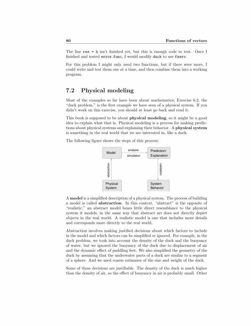
80 Functions of vectors
The line res = h isn’t finished yet, but this is enough code to test. Once Ifinished and tested error func, I would modify duck to use fzero.
For this problem I might only need two functions, but if there were more, Icould write and test them one at a time, and then combine them into a workingprogram.
7.2 Physical modeling
Most of the examples so far have been about mathematics; Exercise 6.2, the“duck problem,” is the first example we have seen of a physical system. If youdidn’t work on this exercise, you should at least go back and read it.
This book is supposed to be about physical modeling, so it might be a goodidea to explain what that is. Physical modeling is a process for making predic-tions about physical systems and explaining their behavior. A physical systemis something in the real world that we are interested in, like a duck.
The following figure shows the steps of this process:
Physical
System
System
Behavior
Prediction/
ExplanationModel
valid
atio
n
simulation
analysis
abstr
action
Amodel is a simplified description of a physical system. The process of buildinga model is called abstraction. In this context, “abstract” is the opposite of“realistic;” an abstract model bears little direct resemblance to the physicalsystem it models, in the same way that abstract art does not directly depictobjects in the real world. A realistic model is one that includes more detailsand corresponds more directly to the real world.
Abstraction involves making justified decisions about which factors to includein the model and which factors can be simplified or ignored. For example, in theduck problem, we took into account the density of the duck and the buoyancyof water, but we ignored the buoyancy of the duck due to displacement of airand the dynamic effect of paddling feet. We also simplified the geometry of theduck by assuming that the underwater parts of a duck are similar to a segmentof a sphere. And we used coarse estimates of the size and weight of the duck.
Some of these decisions are justifiable. The density of the duck is much higherthan the density of air, so the effect of buoyancy in air is probably small. Other
7.3 Vectors as input variables 81
decisions, like the spherical geometry, are harder to justify, but very helpful. Theactual geometry of a duck is complicated; the sphere model makes it possibleto generate an approximate answer without making detailed measurements ofreal ducks.
A more realistic model is not necessarily better. Models are useful because theycan be analyzed mathematically and simulated computationally. Models thatare too realistic might be difficult to simulate and impossible to analyze.
A model is successful if it is good enough for its purpose. If we only need a roughidea of the fraction of a duck that lies below the surface, the sphere model isgood enough. If we need a more precise answer (for some reason) we might needa more realistic model.
Checking whether a model is good enough is called validation. The strongestform of validation is to make a measurement of an actual physical system andcompare it to the prediction of a model.
If that is infeasible, there are weaker forms of validation. One is to comparemultiple models of the same system. If they are inconsistent, that is an indica-tion that (at least) one of them is wrong, and the size of the discrepancy is ahint about the reliability of their predictions.
We have only seen one physical model so far, so parts of this discussion may notbe clear yet. We will come back to these topics later, but first we should learnmore about vectors.
7.3 Vectors as input variables
Since many of the built-in functions take vectors as arguments, it should comeas no surprise that you can write functions that take vectors. Here’s a simple(silly) example:
function res = display_vector(X)
X
end
There’s nothing special about this function at all. The only difference from thescalar functions we’ve seen is that I used a capital letter to remind me that X isa vector.
This is another example of a function that doesn’t actually have a return value;it just displays the value of the input variable:
>> display_vector(1:3)
X = 1 2 3
Here’s a more interesting example that encapsulates the code from Section 4.12that adds up the elements of a vector:
82 Functions of vectors
function res = mysum(X)
total = 0;
for i=1:length(X)
total = total + X(i);
end
res = total;
end
I called it mysum to avoid a collision with the built-in function sum, which doespretty much the same thing.
Here’s how you call it from the Command Window:
>> total = mysum(1:3)
total = 6
Because this function has a return value, I made a point of assigning it to avariable.
7.4 Vectors as output variables
There’s also nothing wrong with assigning a vector to an output variable. Here’san example that encapsulates the code from Section 4.13:
function res = myapply(X)
for i=1:length(X)
Y(i) = X(i)^2
end
res = Y
end
Ideally I would have changed the name of the output variable to Res, as areminder that it is supposed to get a vector value, but I didn’t.
Here’s how myapply works:
>> V = myapply(1:3)
V = 1 4 9
Exercise 7.1 Write a function named find target that encapsulates the code,from Section 4.14, that finds the location of a target value in a vector.
7.5 Vectorizing your functions
Functions that work on vectors will almost always work on scalars as well,because MATLAB considers a scalar to be a vector with length 1.
7.5 Vectorizing your functions 83
>> mysum(17)
ans = 17
>> myapply(9)
ans = 81
Unfortunately, the converse is not always true. If you write a function withscalar inputs in mind, it might not work on vectors.
But it might! If the operators and functions you use in the body of your functionwork on vectors, then your function will probably work on vectors.
For example, here is the very first function we wrote:
function res = myfunc (x)
s = sin(x)
c = cos(x)
res = abs(s) + abs(c)
end
And lo! It turns out to work on vectors:
>> Y = myfunc(1:3)
Y = 1.3818 1.3254 1.1311
At this point, I want to take a minute to acknowledge that I have been a littleharsh in my presentation of MATLAB, because there are a number of featuresthat I think make life harder than it needs to be for beginners. But here, finally,we are seeing features that show MATLAB’s strengths.
Some of the other functions we wrote don’t work on vectors, but they canbe patched up with just a little effort. For example, here’s hypotenuse fromSection 5.5:
function res = hypotenuse(a, b)
res = sqrt(a^2 + b^2);
end
This doesn’t work on vectors because the ^ operator tries to do matrix expo-nentiation, which only works on square matrices.
>> hypotenuse(1:3, 1:3)
??? Error using ==> mpower
Matrix must be square.
But if you replace ^ with the elementwise operator .^, it works!
>> A = [3,5,8];
>> B = [4,12,15];
>> C = hypotenuse(A, B)
C = 5 13 17
84 Functions of vectors
In this case, it matches up corresponding elements from the two input vectors,so the elements of C are the hypotenuses of the pairs (3, 4), (5, 12) and (8, 15),respectively.
In general, if you write a function using only elementwise operators and functionsthat work on vectors, then the new function will also work on vectors.
7.6 Sums and differences
Another common vector operation is cumulative sum, which takes a vectoras an input and computes a new vector that contains all of the partial sums ofthe original. In math notation, if V is the original vector, then the elements ofthe cumulative sum, C, are:
Ci =i∑
j=1
Vj
In other words, the ith element of C is the sum of the first i elements from V .MATLAB provides a function named cumsum that computes cumulative sums:
>> V = 1:5
V = 1 2 3 4 5
>> C = cumsum(V)
C = 1 3 6 10 15
Exercise 7.2 Write a function named cumulative sum that uses a loop tocompute the cumulative sum of the input vector.
The inverse operation of cumsum is diff, which computes the difference betweensuccessive elements of the input vector.
>> D = diff(C)
D = 2 3 4 5
Notice that the output vector is shorter by one than the input vector. As aresult, MATLAB’s version of diff is not exactly the inverse of cumsum. If itwere, then we would expect cumsum(diff(X)) to be X:
>> cumsum(diff(V))
ans = 1 2 3 4
But it isn’t.
7.7 Products and ratios 85
Exercise 7.3 Write a function named mydiff that computes the inverse ofcumsum, so that cumsum(mydiff(X)) and mydiff(cumsum(X)) both return X.
7.7 Products and ratios
The multiplicative version of cumsum is cumprod, which computes the cumula-tive product. In math notation, that’s:
Pi =i∏
j=1
Vj
In MATLAB, that looks like:
>> V = 1:5
V = 1 2 3 4 5
>> P = cumprod(V)
P = 1 2 6 24 120
Exercise 7.4 Write a function named cumulative prod that uses a loop tocompute the cumulative product of the input vector.
MATLAB doesn’t provide the multiplicative version of diff, which would becalled ratio, and which would compute the ratio of successive elements of theinput vector.
Exercise 7.5 Write a function named myratio that computes the inverse ofcumprod, so that cumprod(myratio(X)) and myratio(cumprod(X)) both returnX.
You can use a loop, or if you want to be clever, you can take advantage of thefact that eln a+ln b = ab.
If you apply myratio to a vector that contains Fibonacci numbers, you canconfirm that the ratio of successive elements converges on the golden ratio, (1+√5)/2 (see Exercise 4.6).
7.8 Existential quantification
It is often useful to check the elements of a vector to see if there are any thatsatisfy a condition. For example, you might want to know if there are anypositive elements. In logic, this condition is called existential quantification,
86 Functions of vectors
and it is denoted with the symbol ∃, which is pronounced “there exists.” Forexample, this expression
∃x in S : x > 0
means, “there exists some element x in the set S such that x > 0.” In MATLABit is natural to express this idea with a logical function, like exists, that returns1 if there is such an element and 0 if there is not.
function res = exists(X)
for i=1:length(X)
if X(i) > 0
res = 1;
return
end
end
res = 0;
end
We haven’t seen the return statement before; it is similar to break except thatit breaks out of the whole function, not just the loop. That behavior is what wewant here because as soon as we find a positive element, we know the answer (itexists!) and we can end the function immediately without looking at the rest ofthe elements.
If we exit at the end of the loop, that means we didn’t find what we were lookingfor (because if we had, we would have hit the return statement).
7.9 Universal quantification
Another common operation on vectors is to check whether all of the elementssatisfy a condition, which is known to logicians as universal quantificationand denoted with the symbol ∀ which is pronounced “for all.” So this expression
∀x in S : x > 0
means “for all elements, x, in the set S, x > 0.”
A slightly silly way to evaluate this expression in MATLAB is to count thenumber of elements that satisfy the condition. A better way is to reduce theproblem to existential quantification; that is, to rewrite
∀x in S : x > 0
as
7.10 Logical vectors 87
∼ ∃x in S : x ≤ 0
Where ∼ ∃ means “does not exist.” In other words, checking that all theelements are positive is the same as checking that there are no elements thatare non-positive.
Exercise 7.6 Write a function named forall that takes a vector and returns1 if all of the elements are positive and 0 if there are any non-positive elements.
7.10 Logical vectors
When you apply a logical operator to a vector, the result is a logical vector;that is, a vector whose elements are the logical values 1 and 0.
>> V = -3:3
V = -3 -2 -1 0 1 2 3
>> L = V>0
L = 0 0 0 0 1 1 1
In this example, L is a logical vector whose elements correspond to the elementsof V. For each positive element of V, the corresponding element of L is 1.
Logical vectors can be used like flags to store the state of a condition. They arealso often used with the find function, which takes a logical vector and returnsa vector that contains the indices of the elements that are “true.”
Applying find to L yields
>> find(L)
ans = 5 6 7
which indicates that elements 5, 6 and 7 have the value 1.
If there are no “true” elements, the result is an empty vector.
>> find(V>10)
ans = Empty matrix: 1-by-0
This example computes the logical vector and passes it as an argument to find
without assigning it to an intermediate variable. You can read this versionabstractly as “find the indices of elements of V that are greater than 10.”
We can also use find to write exists more concisely:
88 Functions of vectors
function res = exists(X)
L = find(X>0)
res = length(L) > 0
end
Exercise 7.7 Write a version of forall using find.
7.11 Glossary
top-level function: The first function in an M-file; it is the only function thatcan be called from the Command Window or from another file.
helper function: A function in an M-file that is not the top-level function; itonly be called from another function in the same file.
physical modeling: A process for making predictions about physical systemsand explaining their behavior.
physical system: Something in the real world that we are interested in study-ing.
model : A simplified description of a physical system that lends itself to anal-ysis or simulation.
abstraction: The process of building a model by making decisions about whatfactors to simplify or ignore.
validation: Checking whether a model is adequate for its purpose.
existential quantification: A logical condition that expresses the idea that“there exists” an element of a set with a certain property.
universal quantification: A logical condition that expresses the idea that allelements of a set have a certain property.
logical vector: A vector, usually the result of applying a logical operator to avector, that contains logical values 1 and 0.