Physical and Radiative Characteristics and Long Term Variability of

the Okhotsk Sea Ice Cover

Fumihiko Nishiol, Josefino C. comiso2, Robert erste en^'^, Masashige Nakayama4,

Jinro ukital, A1 ~ a s i e w s k i ~ , Boba stanko5, and Kazuhiro Naokil

1 Center for Environmental Remote Sensing, Chiba University, 1-33 Yayoi-cho, Inage-ku,

Chiba City

2~ryosphere Sciences Branch, NASA Goddard Space Flight Center, Greenbelt, MD

2077 1

3 ~ ~ ~ ~ , Greenbelt, MD 20770

4~okkaido Ice Musuem, Hokkaido, Japan

'NOAA Environmental Research Laboratory, 325 Broadway Ave., Boulder, Colorado,

80303

Submitted to JGR-Oceans

as part of the special section on

"Large Scale Characteristics of the Sea Ice Cover using AMSR-E and other Satellite

Data"

https://ntrs.nasa.gov/search.jsp?R=20080045474 2019-02-15T06:39:02+00:00Z

Abstract

Much of what we know about the large scale characteristics of the Okhotsk Sea ice cover

has been provided by ice concentration maps derived from passive microwave data. To

understand what satellite data represent in a highly divergent and rapidly changing

environment like the Okhotsk Sea, we take advantage of concurrent satellite, aircraft, and

ship data acquired on 7 February and characterized the sea ice cover at different scales

from meters to hundreds of kilometers. Through comparative analysis of surface features

using co-registered data from visible, infrared and microwave channels we evaluated the

general radiative and physical characteristics of the ice cover as well as quantify the

distribution of different ice types in the region. Ice concentration maps from AMSR-E

using the standard sets of channels, and also only the 89 GHz channel for optimal

resolution, are compared with aircraft and high resolution visible data and while the

standard set provides consistent results, the 89 GHz provides the means to observe

mesoscale patterns and some unique features of the ice cover. Analysis of MODIS data

reveals that thick ice types represents about 37% of the ice cover indicating that young

and new ice types represent a large fraction of the ice cover that averages about 90% ice

concentration according to passive microwave data. These results are used to interpret

historical data that indicate that the Okhotsk Sea ice extent and area are declining at a

rapid rate of about -9% and -12 % per decade, respectively.

1. Introduction

The Okhotsk Sea has the unique distinction of being the southernmost region in

the Northern Hemisphere with sea ice cover. The variability of the sea ice cover is thus

sometimes linked closely to the changing climate of the region. It is also among the

world's most productive and richest fishing grounds, in part because of the presence of

sea ice during the winter and spring period. With its high productivity, it is also regarded

as a potential carbon sink. Satellite data revealed the existence of latent as well as

sensible heat polynyas that can have considerable impacts on the physical characteristics

of the sea (Alhltis and Martin, 1987). Furthermore, sea ice is an integral part of the

culture and lives of inhabitants in the coastal regions that surround the sea as manifested

by the existence of several communities along the coastlines and radar stations for

monitoring the ice cover for several decades (e.g., Mombetsu, Japan). Such coverage,

however has been limited and it was not until the advent of satellite remote sensing that

the true nature and extent of the sea ice in the region was revealed. During the satellite

era, large interannual variability and significant decline has been observed (Parkinson et

al., 1999) while anomalies in some years have been associated with El Nino events

(Nishio et al., 1998). A recovery was observed in 2001 but from that time on, the ice

cover has been declining again.

Among the objectives of this study is to utilize data concurrently observed from

aircraft, ship, and sensors from different or the same satellite platforms during the 2003

winter season to provide as comprehensive a characterization of the sea ice cover in the

Okhotsk Sea as possible. Of special interest is the spatial distribution of the different ice

types, especially the different types of new and young ice as well as the thick first year

ice. The strategy is to start with the large scale characteristics as can be inferred from ice

concentration maps derived from passive microwave data. The ice concentration maps

are in turn compared with high resolution satellite data in the visible and infrared to

obtain a general idea how the mesoscale distributions of sea ice is represented in these

ice concentration maps. High resolution aircraft microwave data are analyzed

concurrently with high resolution visible and infrared data to better understand the

passive microwave signature of ice in the region and how and why the derived ice

concentration varies significantly within the pack. These results are in turn used to

interpret the large scale seasonal and interannual variablity as observed from passive

microwave data. Long term changes and trends are also examined in the same context

with a view of gaining insights into what makes the ice cover in the region so variable.

2. The Okhotsk Sea Ice Cover: Large scale and Mesoscale Characteristics

2.1 Satellite Observations

The first Advanced Microwave Scanning Radiometer was launched on board the

EOS-Aqua satellite on 4 May 2002 and is called AMSR-E, while the second one, called

AMSR, was launched on board the Midori-2 satellite on 24 December 2002. The two

systems have very similar specifications, the biggest difference being that AMSR has an

additional 52 GHz channel that is used primarily for atmospheric sounding. Sea ice data

from the two have been compared and provide nearly identical results, the difference

likely associated with changes due to time difference in the equatorial crossing for the

ascending orbits being 13:30 and 22:30 for AMSR-E and AMSR, respectively. AMSR-

E is still in operation while the Midori-2lAMSR ceased operation on 23 October 2003

because of satellite hardware problems. The data used in the comparative study are those

from AMSR-E, only because AMSR was not in full operation when the aircraft and ship

measurements were made. The characteristics of AMSR-E are summarized in Table 1.

As indicated, the resolution varies with frequency with the 89 GHz data having the

highest resolution at 5.4 km. The sensor scans at a fixed incidence angle of 55" with a

swath width of 1445 km covering practically the entire polar region. For long term

variability studies, we make use primarily of historical SMMR and SSWI data for

consistency but we take advantage of almost 5 years overlap of SSWI and AMSR-E to

make the data from these two sensors compatible.

The large scale characteristics of the Okhotsk Sea ice cover on 7 February 2003 as

depicted by an ice concentration map derived from AMSR-E data is presented in Figure

1. Because of the strong contrast in the emissivity between sea ice and open water, the

ice concentration maps provide consistent locations of the ice edges, large divergence

areas, and polynyas (e.g., to the north at around 56" N). Because of daylnight all weather

capabilities, the data is ideal for monitoring large scale seasonal and interannual changes

in the ice cover, as will be illustrated below. Several algorithms have been developed to

estimate ice concentration using different techniques and sets of channels (Svendsen et

al., 1984; Cavalieri et al., 1984; Swift et al., 1986; Comiso, 1986). In this study, we used

data derived from the Bootstrap Algorithm as described in Comiso (2004). AMSR-E

data at high latitudes have been gridded in polar stereographic format at 12.5 by 12.5 km

to take advantage of the improved resolution of the new system. The data have also been

gridded at 25 by 25 km resolution for compatibility with historical passive microwave ice

data. Furthermore, for studies that require optimal resolution, a special data set with 6.25

by 6.25 km resolution has been generated utilizing only the 89 GHz channels (H&V) and

the Bootstrap technique as described in Comiso (2004).

It is fortuitous that on board the Aqua satellite is the Moderate Resolution

Imaging Spectroradiometer (MODIS) which is a 36 channel sensor that covers the

electromagnetic spectrum from 0.405 to 14.385 pm with spatial resolutions of 1 km at

nadir for most channels and at 250 m and 500 m for some special channels. The sensor

scans crosstrack with a swath width of 2,330 km for optimal coverage and good temporal

resolution in the polar region. The visible channels provides the means to discriminate

different surface types including open water, various types of new ice, young ice and

thick ice with snow cover during daytime. The thermal channels provide daylnight

capability and enable estimates of ice concentration as well as the thickness of ice

covered surfaces. During clear skies conditions, MODIS provides valuable information

about the ice cover and at the same time the means to properly interpret the passive

microwave data. The images in Figure 2 shows visible and infrared images from MODIS

for the same day. Unfortunately, for that day, only the Terra/MODIS provided good

clear sky coverage since by the time AquafMODIS passed over the same region four

hours later, there were more clouds in the region. The MODIS data, however, provides a

good overview of how the sea ice cover look like on that date. Compared to the ice cover

as depicted in Figure 1, the images in Figure 2 reveals a lot more details with the visible

and infrared channels providing complementary information. In Figure 1, the marginal

ice zone is represented by a progression of ice concentrations changing from near 100%

to zero % over approximately 100- 150 km region. On the other hand, the MIZ is

represented by MODIS as consisting mainly of ice bands, the widths of which gets

narrower closer to the open sea. With the MODIS data, the unique distributions of

different ice types in the region are also more fully revealed. In this sense, the thermal

infrared data provide information about the thickness of new ice, especially in lead areas.

Figure 3 provides a blown up view of the ice conditions and shows additional details in

the coverage and indicating a different pattern in the infrared for consolidated ice (top

left) than in the relatively loose ice regions. Patterns of large leads in the top left and

thick ice foes in the top middle parts of the image are identified in the image. The

presence of snow cover causes surfaces of different ice types to have basically the same

albedo but the infrared image is able to capture the distribution of the various ice types

with the dark ones representing thick ice floes and the lighter ones representing thinner

ice floes. On the other hand, the banding structure that is revealed in great details in the

visible channel (top right) is not captured by the infrared data mainly because the surfaces

likely have similar temperatures.

Even more detailed information about the spatial distribution and surface

characteristics, of the ice cover can be obtained from Landsat-7data. The Enhanced

Thematic Mapper Plus (ETM+) sensor aboard the satellite has a panchromatic band with

15-m resolution and a thermal infrared band at 60-m resolution. For comparison, the

highest resolution from a MODIS visible channel is 250 m while that for its infrared band

is 1 km. The panchromatic band allows detection of details and improved classification

of surface types especially in narrow lead areas. However, the swath width of Landsat is

only 185 km while that for MODIS is 2330 km providing much less coverage in a single

day. During the aircraft campaign, good Landsat images were obtained on 1 1 February

and some other days but not on 7 February. Thus, comparative studies with aircraft and

ship data during the 7 February campaign will be done mainly with MODIS data while

the Landsat image of 11 February will be compared with near simultaneous AMSR-E

data.

2.2 P3 Aircraft Observations

As part of a dedicated campaign to study the physical and radiative characteristics

of the Okhotsk Sea ice cover, we planned two missions using an instrumented NASA P3

aircraft over selected transects in conjunction with a dedicated ship program as described

below. The first of these missions was successfully implemented but the second one was

not because the aircraft suffered a hardware problem and the latter had to be canceled.

The flight track of the first and only mission over the sea is presented together with an ice

concentration map derived from AMSR-E data in Figure 1. The aircraft went north from

its staging station at the Yokota Airforce Base (near Tokyo) at high altitude (6000),

covered a relatively large area (i.e., 175 by 50 km) at the farthest end, for comparative

studies with satellite data, as shown, and on the way back it went south at low altitude

(1,000 m) to collect data at an even higher resolution. Camera equipments were mounted

for high resolution visible coverage but the most important sensor on board the aircraft is

the Polarimetric Scanning Radiometer (PSR-A) which has frequency channels from 10 to

89 GHz that matches most of those of the AMSR-E sensor. The field-of-view of the

radiometers varies with frequency and at 37 GHz channel, the size of the footprint is

about 240 m at the cruising altitude of 6,000 m while it is about 40 m at 1000 m altitude.

Data from PSR thus allows for more direct comparison with MODIS data and can be

used check the microwave signature of individual features of the pack and also to test the

accuracy of algorithms derived from passive microwave data.

2.3 Ship Observations on board Soya

The physical characteristics of the sea ice cover in the southern portion of the Sea

of Okhotsk (e.g., Ukita et al., 2000) and in other regions (Weeks and Ackley, 1986;

Tucker et al., 1992) have been studied previously. The general location and details of

ship observations in the Okhotsk Sea are described in Naoki et al. (2007). The enlarged

version of the MODIS image shows an ice cover that is made of many ice types including

those of thick first year ice, young ice, gray ice, nilas and pancake ice. It reflects the

dynamic nature of the sea ice cover. The ship study is meant to complement previous

studies and to make measurements that are coincident with measurements from the P3

aircraft and satellite AMSR-E observations.

The ship observation was carried out in the lOOkm range as shown in the general

location presented in Figure 3. When the ship was moving, sea ice conditions around the

ship were recorded with three camcorders installed on the mast, bow and broadside. The

camcorder installed broadside measured the sea ice thickness and other physical

properties of the ice. During periodic stops, ice samples and snow overlying sea ice were

collected directly using a basket.

Typical observations of the ice cover during the cruise are shown in Figures 5a

and 5b. In Figure 5a, rafted ice is shown in the foreground while nilas with some open

water is shown in the middle part. In the background, thick ice cover covers the region

up to the horizon. The image is similar to those observed from the aircraft but with more

details, especially in the rafting geometry. It also represents the usual scenario following

a wind forced event when new and young ice gets rafted and leads open up and turns to

new ice within a few hours. The image in Figure 5b was taken on the same day but for a

different part of the ice cover. In the foreground is the track of the ship that reveals

basically the state of the consolidated ice region. Qualitative analysis indicates that the

ice cover has moderate thickness and the brownish color in some floes reveals the

presence of algae in the underside. The presence of birds in the region indicates that it is

a biologically active region.

Thicknesses of the different types of ice cover were sampled during the and the

results were correlated in a separate paper (Naoki et al., 2007). The microwave signature

of ice of different thicknesses have been shown to be different in part because of varying

salinity and temperature, which were also measured during the cruise.

3. Comparative Analysis using Concurrent Data

3.1 AMSR-E Ice Concentration versus Landsat- 7 Data

The most important geophysical parameter derived from passive microwave data

is likely sea ice concentration. It provides information about the location of the ice edge,

polynyas and divergence areas and is used in the estimates of the extent and area of the

ice cover. It can also be used to estimate how rapidly the ice advances in the winter and

how fast it retreats in the spring and summer. The use of Landsat-7 for process studies is

on the other hand very limited because of sparse coverage and the limit imposed by

daylight and cloud free conditions. When it is available, however, the Landsat-7 data at

15 m resolution provide a wealth of information about the sea ice cover (Steffen and

Maslanik, 1988).

The Landsat visible channel data presented in Figure 6a and taken on 11 February

2003 provides a detailed characterization of the sea ice cover in the Okhotsk Sea. The

albedo of sea ice in the region has been studied by Toyota et al. (1999). The image

indicates the complexity in the spatial distribution and composition of the ice cover at this

time of the year. The ice edge is characterized by the presence of ice bands as indicated

earlier that have been observed to consist mainly of pancake ice usually several cm to a

few meters in diameter. Into the ice pack, some very well defined and thick ice floes are

evident. These thick ice floes are likely the ones that are least altered during the ice

season becoming part of the consolidated ice as the grease ice between them gets totally

frozen. During divergent conditions, they are likely to survive as individual entities again

and during melt period, they are likely to be the last floes to melt in the region. The

presence of a large fraction of new ice (intermediate albedo) in the image is indicative

that the region is in a rapid growth state condition. The stages include the formation tiny

ice particles called frazil ice during super cooling in the upper ocean layer and the

accumulation of these particles at the top surface to form what is usually called "grease

ice." This ice soup solidifies to form nilas or pancake ice depending on sea surface

conditions, leading to either gray ice or larger pancakes and then young ice which is

about 20 to 30 cm in thickness. As the young ice gets thicker and acquires snow cover, it

becomes first year ice which is the dominant ice type during the ice season. Rafting and

ridging of the different ice types due to strong winds are also a natural part of the ice

cover.

The availability of such concurrent images provides the opportunity to examine

how the mesocale characteristics and detailed distribution of different ice types are

represented in the passive microwave data. Ice concentration maps over the same general

area as that in the Landsat image were derived from AMSR-E passive microwave data

using the Bootstrap Algorithm in three grid formats as described earlier: (a) 6.25 km

resolution using the 89 GHz (H & V) data only (Figure 6b); (b) 12.5 km resolution using

the standard set of channels as described by Comiso (2004) (Figure 6c); and (c) 25 km

resolution which is the standard grid for the historical data Figure 6d). It is remarkable

that the basic spatial features are coherent. This is an indication that the visible and

microwave sensors are sensitive to same physical characteristics of the ice cover. It is

apparent that a lot of the detailed distribution of the ice cover provided by Landsat are

also revealed in the AMSR-E image at 6.25 km resolution. The ice edges and divergence

areas are captured by AMSR-E but not the ice bands, mainly because of lack of

resolution in the latter. This implies that for a full characterization of the ice cover,

visible channel data like those from Landsat-7 would be highly desired. The 12.5 km

map provides a respectable representation and shows some of the divergence region

while the 25 km map shows very little in terms of detail. Many of the mesoscale features

that are needed for heat and humidity flux studies are thus lost in the coarse resolution

images.

It is important to point out, however, that for large scale studies, the passive

microwave data provide as good a representation of the ice cover as you can get. A slight

smearing of the ice edge is apparent but the maps provide consistent representation of the

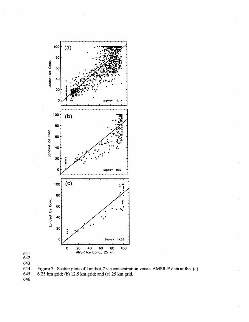
ice cover that is also accurate if resolution is not a factor. A quantitative comparative

analysis is done using the co-registered data sets. Ice concentration is derived from

Landsat-7 data within each of the AMSR-E pixel at the various grids and compared with

data from the latter in Figures 7a, 7b, and 7c for AMSR-E data at 6.25, 12.5 and 25 km

grid, respectively. Linear regression analysis was done on each of these plots and the

regression lines are as shown. Surprisingly, however, the set of data that provided the

best correlation is the 25 km data with the correlation coefficient being 0.90 while

corresponding value when the 12.5 and 6.25 data sets were used are 0.97 and 0,95,

respectively. The comparisons also show a large scatter of the data points with the

standard deviations being about 17.14, 16.0 and 14.2 % ice concentration between

Landsat data and AMSR-E data at 6.25 km, 12.5 km, and 25 km resolutions, respectively.

Part of the reason for the large standard deviation is the few hours difference between the

Landsat-7 coverage and the AMSR-E coverage. Thus, a slight mismatch of the location

of an ice floe affects the correlation and the impact is higher with 6.25 km grid than that

of the 25 km grid. The results of the comparative analysis, however, indicate that despite

the relatively coarse resolution, passive microwave provides a good representation of the

sea ice cover.

This also brings about the issue of what the ice concentration value, as derived

from passive microwave data, really represents. Because the emissivity of sea ice varies

with ice type, it is difficult to categorize the microwave footprint of ice covered areas as

either ice or water. Because new ice has lower emissivities at the different frequencies

and polarizations than thick ice, unless an ice typing can be done effectively, the

algorithm produces ice concentrations that are lower in new ice regions than in thick ice

regions. In the comparative analysis, ice concentration from Landsat was derived based

on the different albedo values with the highest being 100% ice and the lowest being

100% open water. It is apparent that albedo is even more sensitive to thickness than the

emissivity of sea ice.

3.2 PSR versus MODIS

The aircraft PSR data provide the means to compare data of approximately the

same resolution from passive microwave and MODIS. Figure 8 shows data from MODIS

and from PSR at 37 GHz(V), 18 GHz (V), 37 GHz (H), and 89 GHz (V) at the study area

in the north. The MODIS data indicate that the ice cover in the region is mainly

consolidated, with many large ice floes discernible, surrounded by either open water or

new ice. At the top right is part of the Marginal Ice Zone (MIZ) located at the eastern

part of the region (towards the Pacific Ocean, see aircraft track in Figure 1 and top right

in Figure 2). The region is shown to have much lower albedo than the rest of the region,

indicative of the presence of new or younger types of ice cover. The relatively elongated

areas of higher albedo in the region are likely bands of pancakes and surrounded by

newer ice types. Also at the top comer is a pattern suggestive of the presence of clouds

that could pass by the region anytime. It is apparent that the PSR is sensitive to same

general characteristics of the ice cover as the visible channel of MODIS. Except for the

89 GHz channel, a reduction in the brightness temperature in the MIZ is apparent,

especially in the horizontal channel (37 GHz) which exhibits larger contrast between

open ocean and ice covered areas. The 18 GHz channel also show more reduction in

brightness temperature than the 37 GHz channel at vertical polarization because of the

higher contrast in the emissivity of ice and water at lower frequencies. The pattern is not

so obvious with the 89 GHz channel which actually shows lower brightness temperature

within the pack (lower left) than the rest of the region. The aircraft went back and forth

in the region to form the mosaic pattern. Gaps are shown between tracks (see Figure 1)

because the aircraft was going at higher altitude than was originally planned. It took

about an hour for the aircraft to make each track. The 89 GHz data for the second track

(from the right) shows significantly lower brightness temperature than those of the other

tracks suggesting the possibility of an atmospheric effect passing by during the hour the

data were obtained. In the following track, the data apparently went back to normal.

The ice concentration algorithm was applied on the aircraft passive microwave

data and the results are shown in Figure 9. It is apparent that much of the region is

interpreted as basically consolidate (100%) ice with the MIZ and some leads being

retrieved as having concentrations generally between 80 %(light pink) and 95 % (dark

red). In this sense, the passive microwave data captures the basic characteristics of the

ice cover. Again, it does not provide complete information in that it does not capture

some of the features like the presence of large floes and refrozen leads. The "tie points"

for 100% ice can be adjusted in the algorithm (see Comiso, 2004) but it would depend on

what type of sea ice cover would be regarded as 100% ice. This is usually not so easy to

define, as indicated earlier, since during subfreezing temperatures in winter, ice can form

quickly and new ice has emissivity that changes from that of open water to that of thick

ice, depending on thickness.

To gain insights about the signature of the ice cover, several segments of the

northern study area are shown in terms of scatter plots between different channels in

Figures 10, 11, and 12. The specific segments shown in the scatter plots using of passive

microwave data from the PSR are indicated by rectangular boxes in the images at the

bottom. Low albedo values as determined by MODIS are plotted in red to determine how

the lead areas with different thickness of new ice cover are represented in the passive

microwave data. Some but limited variability is apparent at the 10, 19, and 37 GHz

channels at vertical polarization while significantly greater variability is shown for 37

GHz at horizontal polarization and for 89 GHz at both polarizations. The data from the

latter are especially interesting in Figure 11, suggesting that thickness information in lead

areas may be possible to obtain from these channels, especially with the linear trend of

the data from lead areas at the 89 GHz channels. In Figure 12, however, where a large

fraction of the data is of new types of ice, the patterns do not look so linear.

The images in Figure 13 show a comparison of PSR data taken at high altitude

(6000 m, when the aircraft was going north) and at low altitude (1000m, when the aircraft

was going south). The data in the latter provides even improved resolution at around (50

m) when compared to those of the former. The PSR data shown is for the 37 GHz

channel at horizontal resolution. It is apparent that at this resolution, much of the

mesoscale features observed with the MODIS data is captured by the higher resolution

PSR data. It is thus possible that if resolution is not a factor, passive microwave data can

capture much of the mesoscale features that are of interest in polar process studies.

To show relationships of passive microwave data as obtained by PSR with those

from AMSR-E, scatter plots of the various channels over the same ice covered regions

are presented in Figure 14. The column in the left represents plots of various channels

using aircraft data while those in the right represents plots for similar channels but using

AMSR-E data.

3.3. PSR versus Ship Data

The ship tract overlaid on a PSR data at 37 GHz (V) is shown in Figure 15. Ice floes

along the ship tract were sampled in terms of thickness, salinity, snow cover and

temperature. The brightness temperatures at all PSR channels were observed to increase

quite rapidly from near zero thickness to about 10 cm thickness. Between 10 and 20 cm,

the brightness temperatures also increase but more moderately. Beyond 20 cm, the

change in brightness temperature with thickness was no longer discernible. The changes

are more discernible with the horizontal channels than the vertical channels, which is

expected because of the larger contrast in the emissivity of water and ice with the former.

These information were used in conjuction with a model by Naoki et al. (2007), to show

that ice thickness can be inferred from passive microwave data in new ice areas. This

would be a most welcome development especially for heat flux studies.

4. Ice Types, patterns and distribution of sea ice in the Okhotsk Sea

To get a general idea about the distribution of the different types of surfaces in the .

Okhotsk Sea, a classification scheme was applied on the MODIS data in Figure 2a based

on histograms taken in various study areas. The range of albedo for the various types

were assigned arbitrarily according to what was suggested in the histogram study and we

arrived at 1 1 classes that is displayed in different colors in Figure 16. In this scheme,

thick first year ice shown in reds and the pinks represents about 37% of the Okhotsk Sea

ice cover. Young ice shown as brown and yellows represents about 22 % while new ice

shown in greens and blues represents about 28 % of the ice cover. Grease ice andlor

open water shown in gray represent 13%. There was no validation done mainly because

ship data was too limited but the qualitative representation as indicated in Figure 16 looks

reasonable. If the classification is approximately right, it appears that thick ice has the

highest percentage but not a dominant ice cover. This would mean that there is no

sizable core for the ice cover and the extent and area can be easily influenced by

enviromental factors on a year-to-year basis.

5. Seasonal and Interannual Variability and Trends

Monitoring even just the Okhotsk Sea ice cover using concurrent ship, aircraft

and satellite data on a daily basis for about 30 years would be an overwhelming talk that

would require a lot of manpower and money. A more practical way is to use satellite data

and ensuring that the latter are interpreted as accurately as possible. Through

comparative analysis of AMSR-E ice concentration data with co-registered and

concurrent Landsat and MODIS data and also PSR and ship data, we get to better

understand what the ice concentration derived from passive microwave data really means.

We also get a general idea about the distribution of the different ice types. We now try to

use these result to interpret the seasonal and interannual variability of the sea ice cover as

inferred from historical data. To make the latter relevant, we have reprocessed historical

satellite data (SMMR and SSMJI) with the same technique used to process the AMSR-E

data for compatibility in interpretation. During periods of overlap, the ice concentrations

derived from SSMII and AMSR-E have been shown to be very similar. The same

technique were also used to process SMMR data (1978 to 1987) for a longer time series.

The most important variables that can be derived from these ice concentration

maps are sea ice extent and ice area. Sea ice extent is the integrated sum of all areas with

ice concentration of at least 15 % while ice area is the integrated sum of the product of

the area and the ice concentration over all ice covered regions. The daily ice extents and

monthly ice anomalies are presented in Figure 17 while the daily ice areas and monthly

ice area anomalies are presented in Figure 18. The daily extents show the yearly

seasonality of the sea ice cover and how this has varied over the past 28 years. There is

apparently a large interannual variability in the yearly peak values with lows in 1984,

1991, 1997 and 2006 and highs in 1979, 1988, and 2001. Because of large seasonal

variability, trends in the ice cover are difficult to infer from the daily data. A more

standard procedure is to subtract the climatology based on the interannual average of all

available data for each month (e.g., Bjorgo et al., 1997; Cavalieri et al., 1997). The

monthly ice extent anomalies as presented in Figure 17b show large positive anomalies in

the late 1970s and early 1980s and some negative anomalies in the last 3 years.

Regression analysis using this data yielded a trend in ice extent of -8.8% per decade.

Such a trend is quite substantial considering that the overall trends for the entire Arctic

region is about -3% per decade (Parkinson et al., 1999). Similar analyses using ice area

as defined earlier are presented in Figures 18a and 18b. The overall trend in the ice area

is even greater at -12.0 % per decade. Such trend is quite alarming and indicates that the

Sea of Okhotsk is even more vulnerable in loosing its ice cover than the perennial ice

cover in the Arctic as reported in Comiso (2002), and Stroeve et a1.(2004) and updated in

Comiso (2006). To gain insights into this trend, the length of each ice season from 1979

to the present were inferred from daily data and the results are presented in Figure 19.

The trend is more modest showing declines of about 2 to 4 days per decade. The latter

may not mean much because the ice cover is seasonal ice and it takes only subfreezing

temperatures to create sea ice. The region is usually below freezing during the winter

period. An early or late start date is therefore not as significant as the observed decline

in ice extent and ice area since the latter suggest warmer winter temperatures. It is

warmer winter temperatures that could lead to lower rate of fi-eeze-up which means less

extensive ice cover. There are other complications including the composition of the ice

cover as discussed in the next section.

6. Discussion and Conclusions

The Sea of Okhotsk has the potential of providing an important signal about the

changing global climate since it is the southernmost region in the Northern Hemisphere

with an ice cover. We have been using passive microwave ice concentration data to

monitor the ice cover in the region but the latter is difficult to interpret especially in a

very divergent and rapidly changing environment like the Sea of Okhotsk. In this study,

we examined the general physical and radiative characteristics of the sea ice cover in the

Okhotsk Sea using concurrent in situ, aircraft and satellite data. High resolution satellite

data reveal a complex distribution of the ice cover with only about 37% .being covered by

thick ice types and the rest being young and new ice, the signature of which can be very

unpredictable. They show many complex features in the ice cover that cannot be

represented in the standard passive microwave data sets. With data from the recently

launched AMSR-E sensor, many of such mesoscale features are adequately represented,

especially in the 89 GHz images, making the latter a useful tool for polar process studies.

However, the data has to be used with care since data at this wavelength is sensitive to

atmospheric and snow cover effects. The standard sea ice data from passive microwave

at 12.5 krn resolution shows some of the mesoscale features as well but much of the

features are lost in the 25 km grids. Our results, however, show that the 25 km grid

provides dependable ice cover data that can be combined with historical data to study the

state and fhture of the ice cover.

The results of our analysis of historical data show that the sea ice cover in the

Okhotsk Sea is declining at a rapid rate of -8.8 and -12.0 % per decade for sea ice extent

and ice area, respectively. Such trend is alarming especially since the region is a very

productive region in part because of the presence of sea ice. Since the Okhotsk Sea ice

cover has a relatively small fraction of thick ice (about 37%) and the average

concentration of ice in the Okhotsk Sea is about 90%, a large fraction of the consolidated

ice consists of young and new ice. The ice cover has actually declined in a similar way in

the 1990s. The lack of a strong dependable core of thick ice that provides stability in the

ice cover could mean that the year-to-year variability can easily be attributed by

environmental forcing such as wind strength and direction during winter and spring. The

higher decline in ice area compared to that of the ice extent also indicates that the region

is getting more divergent with the average concentrations getting lower with time. What

this implies in the context of a warming Arctic is not known and will be the subject for

future studies. What we know is that the length of the ice season has been declining but

only by about 2 to 4 days per decade. Such change is not sufficient to explain the high

rate of decline since the entire region is in sub-freezing temperatures during the winter

months. Further studies are needed especially since the observed high rate of decline in

ice extent and ice area may mean that the rate of ice production in the region is declining

on account of a warmer winter.

495 Table 1. AMSR-E Sensor Characteristics

References

Alfultis, M.A. and S. Martin, Satellite passive microwave studies of the Sea of Okhotsk

ice cover and its relation to oceanic processes, 1978-1982, J. Geophys. Res., 92,

13,013-13,028, 1987.

Bjorgo, E. , O.M. Johannessen, and M.W. Miles, "Analysis of merged SSMR-SSM/I

time series of Arctic and Antarctic sea ice parameters 1978-1995," Geophys. Res.

Lett., Vol. 24, pp. 4 13-416, 1997.

Cavalieri, D.J., P. Gloersen, W.J. Campbell, Determination of sea ice parameters with the

Nimbus7 SMMR, J. Geophys Res., 89, 5355-5369,1984.

Cavalieri, D.J., P. Gloersen, C. Parkinson, J. Comiso, and H.J. Zwally, Observed

hemispheric asymmetry in global sea ice changes, Science, 2 78(7), 1 104- 1 106,1997.

Comiso, J. C., Characteristics of winter sea ice from satellite multispectral microwave

observations, J. Geophys. Rev., 91(C1), 975-994, 1986.

89.0

0.34 cm

H & V

6.0x4.9

5.4

1.1

1.3

0.18

Freq. GHz)

Wavelength

Polarization

IFOV (km)

Mean Res.

(km)

Sens (K)

Int. time

(msec)

Beamwidth

("1 Swath

Width

Satellite

Altitude

6.9

4.3 cm

H & V

73.0x43.1

56

0.3

2.6

2.2

1445 km

705 km

18.7

1.6 cm

H & V

26.2x16.5

2 1

0.6

2.6

0.8

10.65

2.8 cm

H & V

49.8x29.6

38

0.6

2.6

1.4

23.8

1.27 cm

H & V

30.8x19.0

24

0.6

2.6

0.9

36.5

0.82 cm

H & V

13.7x10.3

12

0.6

2.6

0.4

Comiso, J. C., A rapidly declining Arctic perennial ice cover, Geophys Res. Letts.,

29(20), 1956, doi:l 0.1029/2002GL015650, 2002.

Comiso, J.C., Sea ice algorithm for AMSR-E, Rivista Italiana di Telerilevamento (Italian

Journal of Remote Sensing), 30/31, 1 19-130,2004.

Comiso, J. C., Abrupt Decline in the Arctic Winter Sea Ice Cover, Geophys. Res. Lett.,33,

L18504, doi: lO.l029/2006GL02734 1,2006.

Comiso, J. C., D. J. Cavalieri, and T. Markus, Sea ice concentration, ice temperature, and

snow depth, using AMSR-E data, IEEE TGRS, 41(2), 243-252,2003.

Matzler, C., R. 0 . Ramseier, and E. Svendsen, "Polarization effects in sea ice

signatures," IEEE J. Oceanic Engineering, Vol. OE-9, pp. 333-338, 1984.

Naoki, K. J. Ukita, F. Nishio, M. Nkayama, J. Comiso and A. Gasiewski, Thin sea ice

thickness as inferred from passive microwave and in situ observations, J. Geophys.

Res. (2007, submitted).

Nishio, F. M. Aota, and K. Cho, Variability of se ice extent in the Okhotsk Sea,

Proceedings of the Sea of Okhotsk Symposium, pp. 1-4, 1998.

Parkinson, C.L., D.J Cavalieri, P. Gloersen, H.J. Zwally, and J.C. Comiso, Arctic sea ice

extents, areas, and trends, 1978-1996, J. Geophys. Res., 104(C9), 20837-20856, 1999.

Steffen, K. and J.A. Maslanik, Comparison of Nimbus 7 Scanning Multichannel

Microwave Radiometer radiance and derived sea ice concentrations with Landsat

imagery for the north water area of Baffin Bay, J. Geophys. Res., 93(C9), 10,760-

10,781, 1988.

Stroeve, J.C., M.C., Serreze, F. Fetterer, T. Arbetter, M. Meier, J. Maslanik and K.

Knowles, Tracking the Arctic's shrinking ice cover: Another extreme September

minimum in 2004, Geophys. Res. Lett. 32, doi: 10.1029/2004GL02 18 10,2004.

Svendsen, E., C. Matzler, T.C. Grenfell, "A model for retrieving total sea ice

concentration from a spaceborne dual-plarized passive microwave instrument

operating near 90 GHz," Int. J. Rem. Sens., Vol. 8, pp. 1479-1487, 1987.

Swift, C.T., L.S. Fedor, and R.O. Ramseier, An algorithm to measure sea ice

concentration with microwave radiometers, J. Geophys. Res., 90(Cl), 1087- 1099,

1985.

Toyota, T. , J. Ukita, K.I. Ohshima, M. Wakatsuchi and K. Muramoto, A measurement of

sea ice albedo over the southwestern Okhotsk Sea, J. Meteor. Soc. Japan, 77, 117-

133, 1999.

Tucker, W.B., D.K. Perovich, and A.J. Gow, "Physical properties of sea ice relevant to

remote sensing," Chapter 2, Microwave Remote Sensing of Sea Ice, (ed. by Frank

Carsey), American Geophysical Union, Washington, D.C., 9-28, 1992.

Ukita, J., T. Kawamura, N. Tanaka, T. Toyota, and M. Wakatsuchi, Physical and stable

isotopic properties and growth processes of sea ice collected in the southern Sea of

Okhotsk, J. Geophys. Res., 105, 22083-22093,2000.

Vant, M.R., R.B. Gray, R.O. Ramseier, and V. Makios. 1974. Dielectric properties of

fresh and sea ice at 10 and 35 GHz, J. AppliedPhysics, 45(11), 4712-4717.

Weeks, W.F., and S. F. Ackley, The growth, structure and properties of sea ice, The

Geophysics of Sea Ice, edited by N. Unterstiener, pp. 9-164, NATO ASI Ser.B, vol.

146, Plenum, New York, 1986.

List of Figures

Figure 1. AMSR-E ice concentration map of the Okhotsk Sea showing the P3 aircraft

track on 7 February 2003.

Figure 2. MODIS image of the Okhotsk Sea ice cover on 7 February 2003 in the (a)

visible and (b) infrared channels with general locations of coastal and sensible heat

polynya.

Figure 3. Enlarged MODIS image of the Okhotsk Sea ice cover on 7 February 2003 in

the (a) visible and (b) infrared channels.

Figure 4. Aerial photograph of (a) new ice and (b) thick ice floes in the Okhotsk Sea on 7

February 2003 as taken from the P3 aircraft.

Figure 5. Typical sea ice cover of (a) rafted ice and grease ice and (b) broken thick ice as

observed from the ship

Figure 6. Landsat-7 visible channel data and AMSR-E ice concentration images using (a)

6.25 km; (b) 12.5 km; and (c) 25 krn resolution data.

Figure 7. Scatter plots of Landsat-7 versus AMSR-E data at a resolution of (a) 6.25 krn;

(b) 12.5 km; and (c) 25 krn.

Figure 8. MODIS image in the northern region and corresponding PSR data at 37

GHz(V), 18 GHz (V), 37 GHz (H), and 89 GHz (V).

Figure 9. PSR data converted to ice concentration and corresponding MODIS data.

Figure 10. Scatter plots of 10 GHz (V) versus 37 GHz (V); 19 GHz (V) vs 37 GHz (V);

37 GHz (H) vs 37 GHz (V) and 89 GHz (H) vs 89 GHz (V). The red data points

represent low albedo areas inside the box in the image below the plots. The box is in a

divergence region.

Figure 11. Scatter plots of 10 GHz (V) versus 37 GHz (V); 19 GHz (V) vs 37 GHz (V);

37 GHz (H) vs 37 GHz (V) and 89 GHz (H) vs 89 GHz (V). The red data points

represent low albedo areas inside the box in the image below the plots. The box is in a

consolidated ice region.

Figure 12. Scatter plots of 10 GHz (V) versus 37 GHz (V); 19 GHz (V) vs 37 GHz (V);

37 GHz (H) vs 37 GHz (V) and 89 GHz (H) vs 89 GHz (V). The red data points

represent low albedo areas inside the box in the image below the plots. The box is in the

marginal ice zone.

Figure 13. MODIS image and PSR data at high (6000m) and low (1000m) altitudes with

the latter showing even higher resolution than MODIS data.

Figure 14. Scatter plots comparing aircraft data with AMSR-E data

Figure 15. Ship track on the PSR data on 7 February 2003

Figure 16. Ice class map using MODIS visible channel data. Red and pink represent

thick ice, brown and yellow represent young ice, while green and blues represent new ice.

Gray represents either grease ice or open water.

Figure 17. (a) Seasonal and interannual variability of the ice extent of the Sea of Okhotsk

and Sea of Japan; (b) Anomalies and trends in the ice extent of the Sea of Okhotsk ice

cover

Figure 18. (a) Seasonal and interannual variability of the ice area of the Sea of Okhotsk

and Sea of Japan; (b) Anomalies and trends in the ice area of the Sea of Okhotsk ice

cover.

Figure 19. Length of the ice season in the Okhotsk Sea from 1978 to 2005 (blue) and the

width at half-height of the plots in Figure 18a.

605 606 607 608 609 Figure 1 AMSR-E ice concentration map of the Sea of Okhotsk on 7 February 2003 and flight track of the 6 10 aircraft mission on the same day.

Figure 2. MODIS image of the Okhotsk Sea ice cover on 7 February 2003 in the (a) visible (6 pm) and (b) thermal infrared (1 1 pm) channels of AquaMODIS sensor.

Fig. 3 Enlarged MODIS image of the Okhotsk and (b) thermal infrared (1 1 pm) channels of Aqi

\

thick Ice floes

Sea ice cover in the (a) visible (6 pm) udMODIS sensor.

625 626 Figure 4. Typical (a) new ice and (b) thick ice floes in the Okhotsk Sea as viewed from the P3 627 Aircraft 62 8 629 630

632 633 Figure 5. Sample photographs of sea ice from ship of (a) rafted and grease ice; and (b) broken thick 634 ice in the Okhotsk Sea 63 5

63 6 63 7 638 Figure 6 Landsat-7 image of the Okhotsk Sea ice cover and corresponding AMSR-E ice 639 concentration map at the (a) 6.25 km grid; (b) 12.5 km grid; and (c) 25 krn grid. 640

0 20 40 60 80 1 0 0 AMSR Ice Conc.. 25 krn

Figure 7. Scatter plots of Landsat-7 ice concentration versus AMSR-E data at the (a) 6.25 km grid; (b) 12.5 km grid; and (c) 25 km grid.

;igure 8. MODIS image in the 7 GHz (H) and 89 GHz (V).

northern regiot 1 and PSR data _ at 37 GHz(V), 18 GHz (V),

Figure 9. PSR ice concentration data (in color) derived using the Bootstrap Algorithm and MODIS data (in black and white). Color scale is the same as in Figure 1.

Sea of Okhotsk (Feb 7, 2004)

656 657 Figure 10. Scatter plots of 10 GHz (V) versus 37 GHz (V); 19 GHz (V) vs 37 GHz (V); 658 37 GHz (H) vs 37 GHz (V) and 89 GHz (H) vs 89 GHz (V). The red data points 659 represent low albedo areas inside the box in the image below the plots. The box is in a 660 divergence region.

Sea of Okhotsk (Feb 7, 2004)

662 663 Figure 11. Scatter plots of 10 GHz (V) versus 37 GHz (V); 19 GHz (V) vs 37 GHz (V); 664 37 GHz (H) vs 37 GHz (V) and 89 GHz (H) vs 89 GHz (V). The red data points 665 represents low albedo areas inside the box in the image below the plots. The box is in a 666 consolidated ice area. 667

Seo of Okhotsk (Feb 7 , 2004)

668 669 670 Figure 12. Scatter plots of 10 GHz (V) versus 37 GHz (V); 19 GHz (V) vs 37 GHz (V); 67 1 37 GHz (H) vs 37 GHz (V) and 89 GHz (H) vs 89 GHz (V). The red data poits 672 represents low albedo areas inside the box in the image below. The box is in a marginal 673 ice zone region. 674

Figure 13. (b) MODIS image over image with PSR high (6000 m) and Sea.

the Okhotsk Sea on 7 February 2003; and (b) MODIS low altitude (1000 m) data at 37 GHz over Okhotsk

Y r n a

dm f ,

$50 IUI 200 210 240 2eo IbD M O I Z O H O ~ 2 W

P-J 0s-rrrbn

mm1402M28m M O t t O 2 4 0 2 6 0 m 680 JX P-J 3%

68 1 682 Figure 14 Scatter plots comparing PSR and AMSR-E data 683

685 686 Figure 15. Ship track on the PSR data on 7 February 2003

Figure 16. Ice class map using MODIS visible cha thick ice, brown and yellow represent young ice, w Gray represents either grease ice or open water.

.nnel d hile gr

ata. seen

Red and pink and blues rep1

repre .esent

sent new ice.

Seas of Okhotsk m d Jopon 2.0

1.0

a E 0.5 Y * 0 .- V

& 0.0 C fD 4

X W

$ -0.5 -

-1.0

693 78 80 82 84 86 88 90 92 94 96 98 00 02 04 06

694 695 Figure 17. (a) Seasonal and interannual variability of the ice extent of the Sea of Okhotsk 696 and Sea of Japan from 1978 to 2006; (b) Anomalies and trends in the ice extent of the Sea 697 of Okhotsk ice cover from 1978 to 2006. 698

-1.0

699 78 80 82 04 86 88 90 92 94 96 98 00 02 04 06 700 701 Figure 18. (a) Seasonal and interannual variability of the ice area of the Sea of Okhotsk 702 and Sea of Japan fiom 1978 to 2006; and (b) Anomalies and trends in the ice area of the 703 Sea of Okhotsk ice cover from 1978 to 2006. 704

300

250

200

QI e 150 Q

100 Y - - -

SCT Futr LC.. Season : -0.2 i 0 3 & y s / ~

-0.9 t r 25 X/drrc

-3.4 t 2.7 X/ch O - i . . . . f . . . . l . . . . t . . . . l * * . . t

t 980 1985 1990 1995 2000 2005 705 706 Figure 19. Length of the ice season in the Okhotsk Sea from 1978 to 2005 (blue) and the 707 width at half-height of the plot in Figure 18a.