1

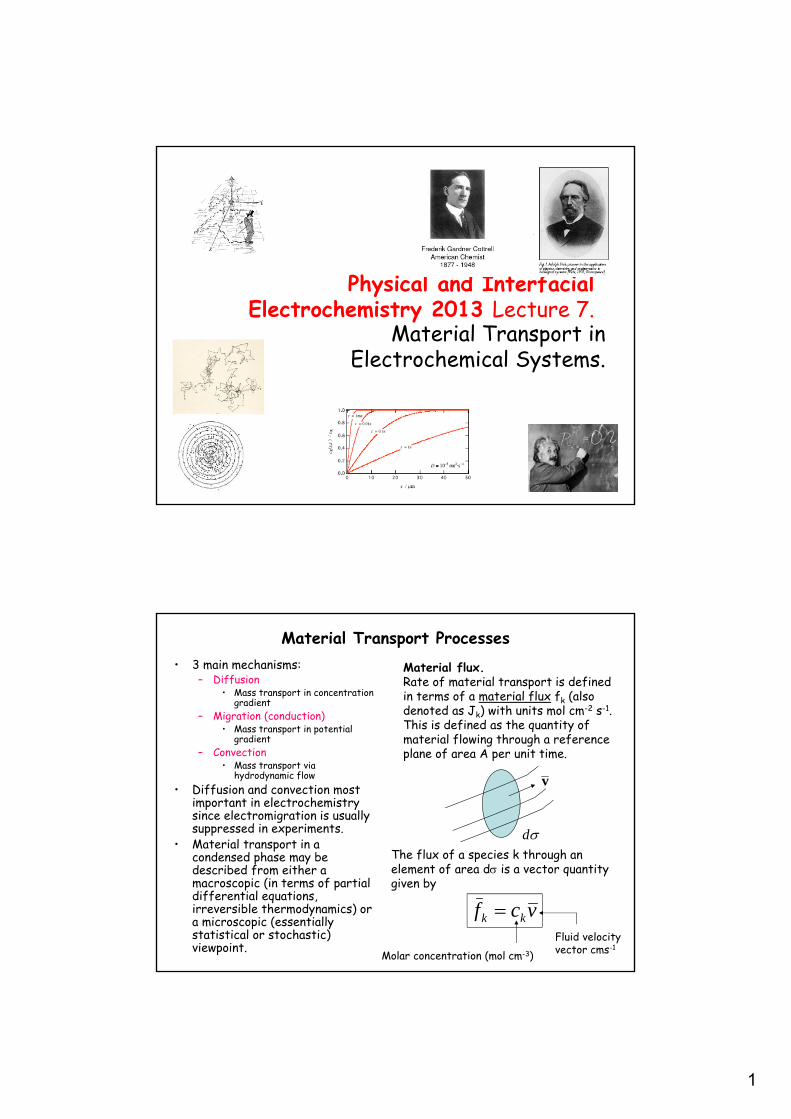
Physical and Interfacial Electrochemistry 2013 Lecture 7.

Material Transport in Electrochemical Systems.

Material Transport Processes• 3 main mechanisms:

– Diffusion• Mass transport in concentration

gradient– Migration (conduction)

• Mass transport in potential gradient

– Convection• Mass transport via

hydrodynamic flow• Diffusion and convection most

important in electrochemistry since electromigration is usually suppressed in experiments.

• Material transport in a condensed phase may be described from either a macroscopic (in terms of partial differential equations, irreversible thermodynamics) or a microscopic (essentially statistical or stochastic) viewpoint.

Material flux.Rate of material transport is definedin terms of a material flux fk (alsodenoted as Jk) with units mol cm-2 s-1.This is defined as the quantity of material flowing through a referenceplane of area A per unit time.

v

dThe flux of a species k through an element of area d is a vector quantity given by

vcf kk

Molar concentration (mol cm-3)

Fluid velocityvector cms-1

2

Diffusive Material TransportDiffusive material transport driven by presence of concentration gradient.Mathematically described by the Fick Diffusion equations (material flowexpressions directly analogous to Fourier heat flow (energy transfer in atemperature gradient) expressions.Macroscopically, mathematical expressions previously developed for heat flow can be used with suitable modification to corresponding material transport problem.

High soluteconcentration

Low soluteconcentration

Net diffusive flux

Assume driving force for diffusionis proportional to chemical potential gradient.

We consider two cases: steady state (timeindependent) diffusion and transient (timedependent) diffusion. In the first case c = c(x)only whereas in the second case c = c(x,t).

We introduce a diffusive pseudo-drivingforce FD which is related to the gradientin chemical potential via:

kD k

D k k

dF c

dxF c

1-D

3-D

Steady State Fickian Diffusion.A.E Fick1829-1901

http://en.wikipedia.org/wiki/Adolf_Eugen_Fickhttp://en.wikipedia.org/wiki/Fick's_law_of_diffusion

We now assume that diffusive pseudo force FD is associated with a diffusiveFlux f which serves as a measure of the diffusion rate.We use irreversible thermodynamics to relate flux and force:

....2 DDk FFf

Assuming FD is small corresponding to small departure from equilibrium(linear irreversible thermodynamics) we neglect terms in FD

2 and higher. AlsoSince if FD = 0 then fk = 0 (no effect exists without the corresponding cause) then = 0. This leaves us with the assignment that we have a linear relationship betweenFlux (the effect) and driving force (the cause):

kk D k

df F c

dx

0 ln

ln

k k k

k k k k

k k k

k

RT a

a c c

d d c dcRTRT

dx dx c dx

kk D k

k kk

k

df F c

dx

dc dcRTc RT

c dx dx

Ideal solution approximationActivity coefficient = 1.

We introduce the phenomenological diffusion coefficient (unit: cm2s-1) D

RTD

Introducing the definition of chemical potential:

We arrive at the Fick equationof steady state diffusion: kkk

kkk

cDfdx

dcDf

1-D

3-D

3

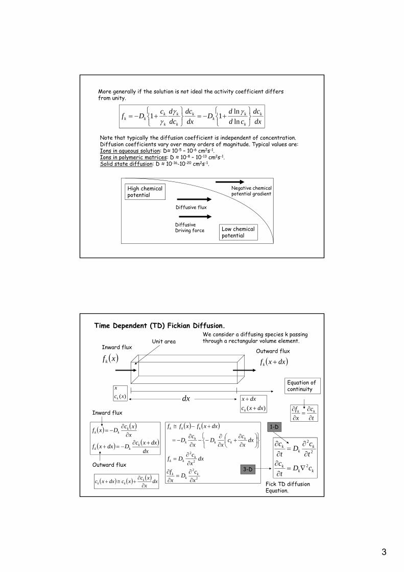
More generally if the solution is not ideal the activity coefficient differsfrom unity.

dx

dc

cd

dD

dx

dc

dc

dcDf k

k

kk

k

k

k

k

kkk

ln

ln11

Note that typically the diffusion coefficient is independent of concentration.Diffusion coefficients vary over many orders of magnitude. Typical values are:Ions in aqueous solution: D≈ 10-5 – 10-6 cm2s-1.Ions in polymeric matrices: D ≈ 10-8 – 10-13 cm2s-1.Solid state diffusion: D ≈ 10-16-10-20 cm2s-1.

High chemicalpotential

Low chemicalpotential

Diffusive flux

Negative chemicalpotential gradient

DiffusiveDriving force

Time Dependent (TD) Fickian Diffusion.

Inward flux

xfk

Outward flux

dxxfk

)(xc

x

k

)( dxxc

dxx

k

Unit area

dx

We consider a diffusing species k passingthrough a rectangular volume element.

dx

dxxcDdxxf

x

xcDxf

kkk

kkk

Inward flux

Outward flux

dx

x

xcxcdxxc k

kk

2

2

2

2

x

cD

x

f

dxx

cDf

dxx

cc

xD

x

cD

dxxfxff

kk

k

kkk

kkk

kk

kkk

Equation of continuity

t

c

x

f kk

kkk

kk

k

cDt

ct

cD

t

c

2

2

2

1-D

3-D

Fick TD diffusionEquation.

4

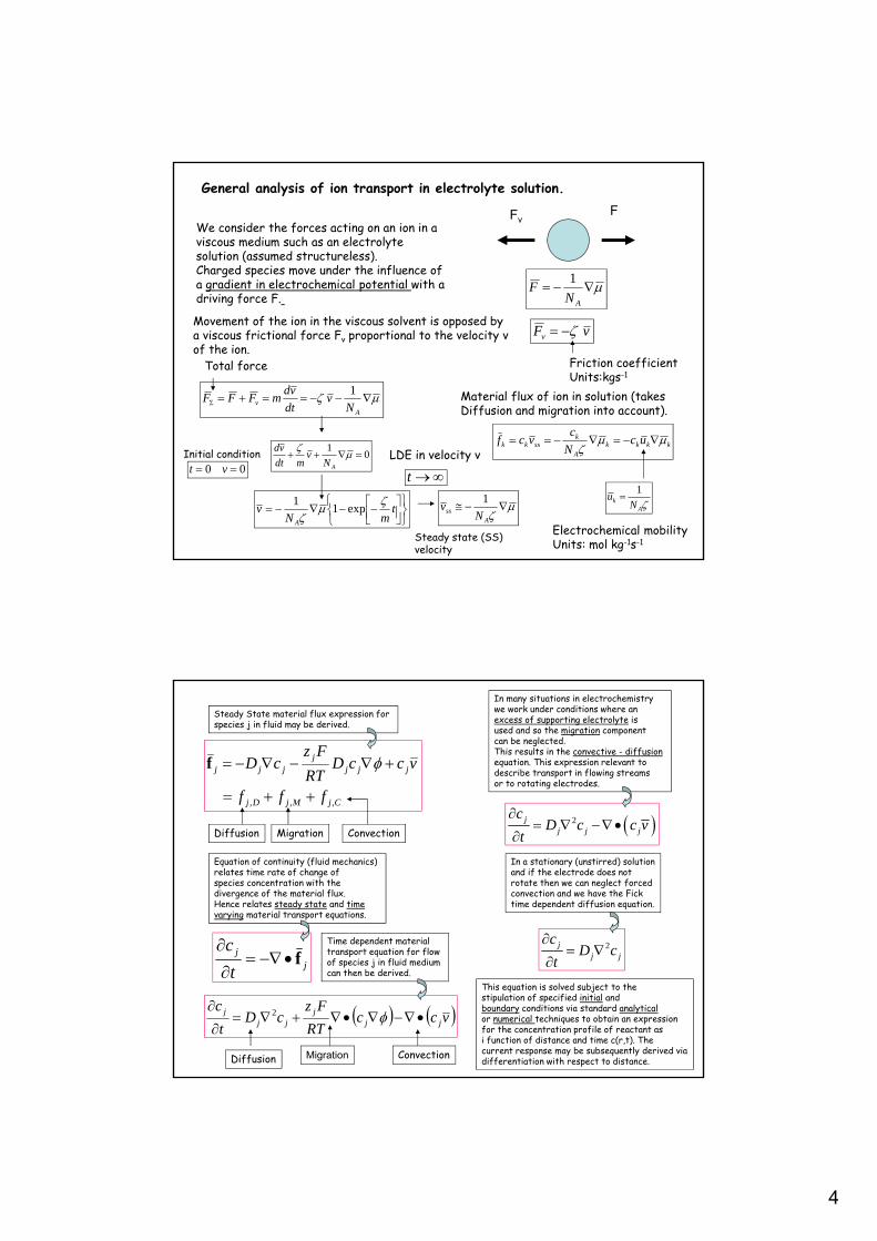
General analysis of ion transport in electrolyte solution.FFv

We consider the forces acting on an ion in aviscous medium such as an electrolytesolution (assumed structureless).Charged species move under the influence ofa gradient in electrochemical potential with adriving force F.

AN

F1

Movement of the ion in the viscous solvent is opposed bya viscous frictional force Fv proportional to the velocity vof the ion.

vFv

Friction coefficientUnits:kgs-1

A

v Nv

dt

vdmFFF

1

Total force

LDE in velocity v

t

mNv

A

exp11

00 vt0

1

ANv

mdt

vdInitial condition

Ass N

v1

t

Steady state (SS) velocity

Material flux of ion in solution (takesDiffusion and migration into account).

kkkkA

ksskk uc

N

cvcf

Ak N

u1

Electrochemical mobilityUnits: mol kg-1s-1

Steady State material flux expression for species j in fluid may be derived.

CjMjDj

jjjj

jjj

fff

vccDRT

FzcD

,,,

f

jj

t

cf

vccRT

FzcD

t

cjj

jjj

j

2

Time dependent material transport equation for flow of species j in fluid mediumcan then be derived.

Diffusion Migration Convection

Equation of continuity (fluid mechanics) relates time rate of change of species concentration with the divergence of the material flux.Hence relates steady state and timevarying material transport equations.

Diffusion Migration Convection

In many situations in electrochemistrywe work under conditions where anexcess of supporting electrolyte isused and so the migration componentcan be neglected.This results in the convective - diffusionequation. This expression relevant todescribe transport in flowing streamsor to rotating electrodes.

2jj j j

cD c c v

t

In a stationary (unstirred) solutionand if the electrode does notrotate then we can neglect forcedconvection and we have the Ficktime dependent diffusion equation.

2jj j

cD c

t

This equation is solved subject to thestipulation of specified initial andboundary conditions via standard analyticalor numerical techniques to obtain an expressionfor the concentration profile of reactant asi function of distance and time c(r,t). Thecurrent response may be subsequently derived viadifferentiation with respect to distance.

5

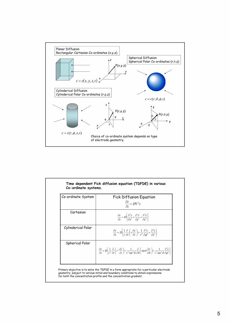
Planar DiffusionRectangular Cartesian Co-ordinates (x,y,z).

tzyxcc ,,,x

y

z

Cylinderical DiffusionCylinderical Polar Co-ordinates (r,,z)

r

P(r,,z)

z y

z

x

),,,( tzrcc

Spherical DiffusionSpherical Polar Co-ordinates (r,,)

P(r,,)r

z

yx

),,,( trcc

P(x,y,z)

Choice of co-ordinate system depends on typeof electrode geometry.

Co-ordinate System Fick Diffusion Equation

Cartesian

Cylinderical Polar

Spherical Polar

2

2

2

2

2

2

z

c

y

c

x

cD

t

c

2

2

2

2

2

11

z

cc

rr

cr

rrD

t

c

2

2

22222

2 sin

1sin

sin

11

c

r

c

rr

cr

rrD

t

c

cDt

c 2

Time dependent Fick diffusion equation (TDFDE) in variousCo-ordinate systems.

Primary objective is to solve the TDFDE in a form appropriate for a particular electrode geometry, subject to various initial and boundary conditions to obtain expressions for both the concentration profile and the concentration gradient.

6

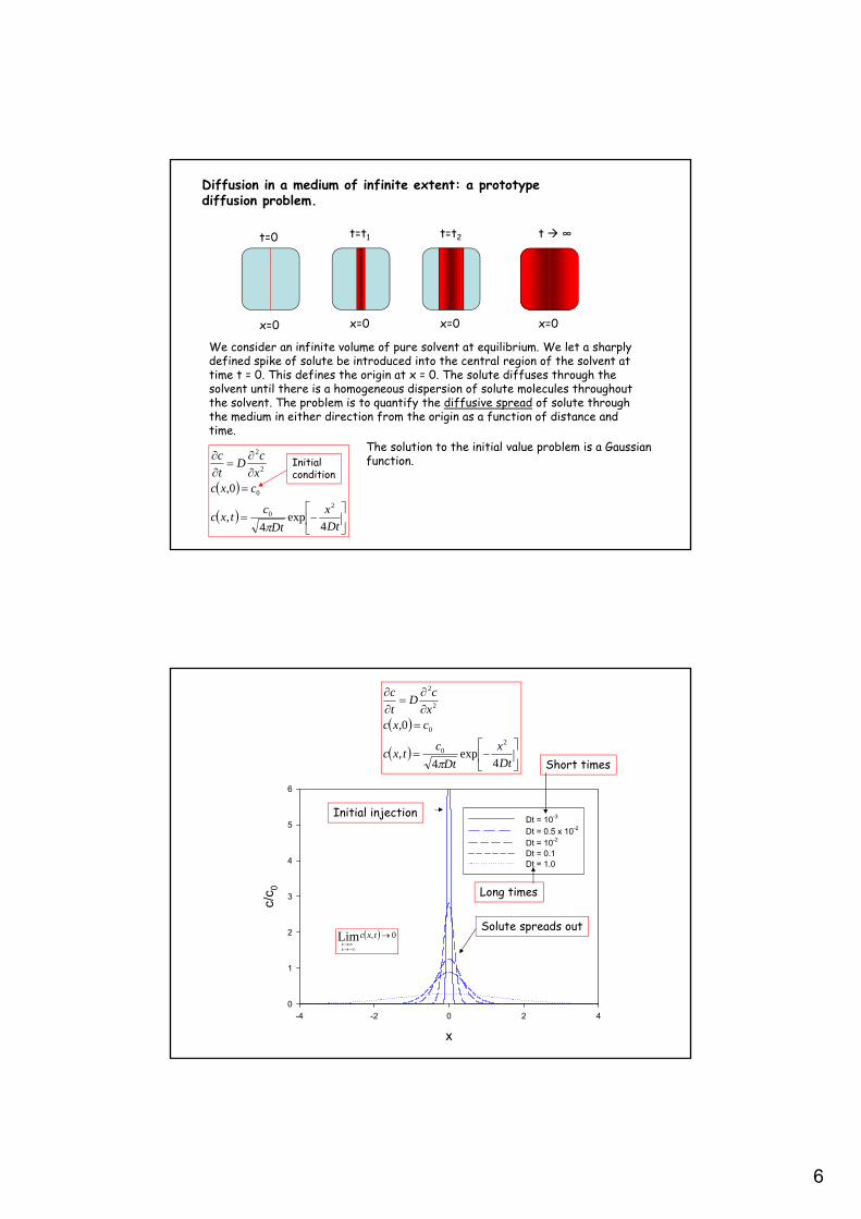
Diffusion in a medium of infinite extent: a prototypediffusion problem.

x=0 x=0 x=0 x=0

t=0 t=t1 t=t2 t ∞

We consider an infinite volume of pure solvent at equilibrium. We let a sharplydefined spike of solute be introduced into the central region of the solvent attime t = 0. This defines the origin at x = 0. The solute diffuses through thesolvent until there is a homogeneous dispersion of solute molecules throughoutthe solvent. The problem is to quantify the diffusive spread of solute throughthe medium in either direction from the origin as a function of distance andtime.

Dt

x

Dt

ctxc

cxcx

cD

t

c

4exp

4,

0,2

0

0

2

2

Initial condition

The solution to the initial value problem is a Gaussianfunction.

x

-4 -2 0 2 4

c/c 0

0

1

2

3

4

5

6

Dt = 10-3

Dt = 0.5 x 10-2

Dt = 10-2

Dt = 0.1Dt = 1.0

Dt

x

Dt

ctxc

cxcx

cD

t

c

4exp

4,

0,2

0

0

2

2

Initial injection

Solute spreads out

Short times

Long times

0,Lim

txc

xx

7

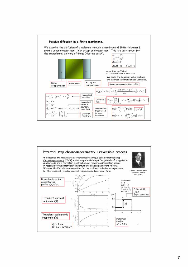
Passive diffusion in a finite membrane.

We examine the diffusion of a molecule through a membrane of finite thickness Lfrom a donor compartment to an acceptor compartment. This is a basic model forthe transdermal delivery of drugs (nicotine patch).

Donorcompartment

Acceptorcompartment

membrane

L 0,,0

00,

2

2

tLcctc

xcx

cD

t

c

= partition coefficientc∞ = concentration in membrane

We scale the boundary value problem and express in dimensionless variables.

2

2

2

1

,0 0 0, 1 1, 0

c x Dtu

c L L

u u

u u u

f L u

Dc

DiffusionFlux (rate)

Normalisedvariables

Normalised Initial & boundary conditions

22

1

exp1sin

21, nn

nu

n

1

22

1

exp121n

n nu

1

2222

0

exp1

2n

n

L nn

dN

N

61L

Membrane concentration profile

Diffusiveflux

Total amounttransferredthroughMembrane.

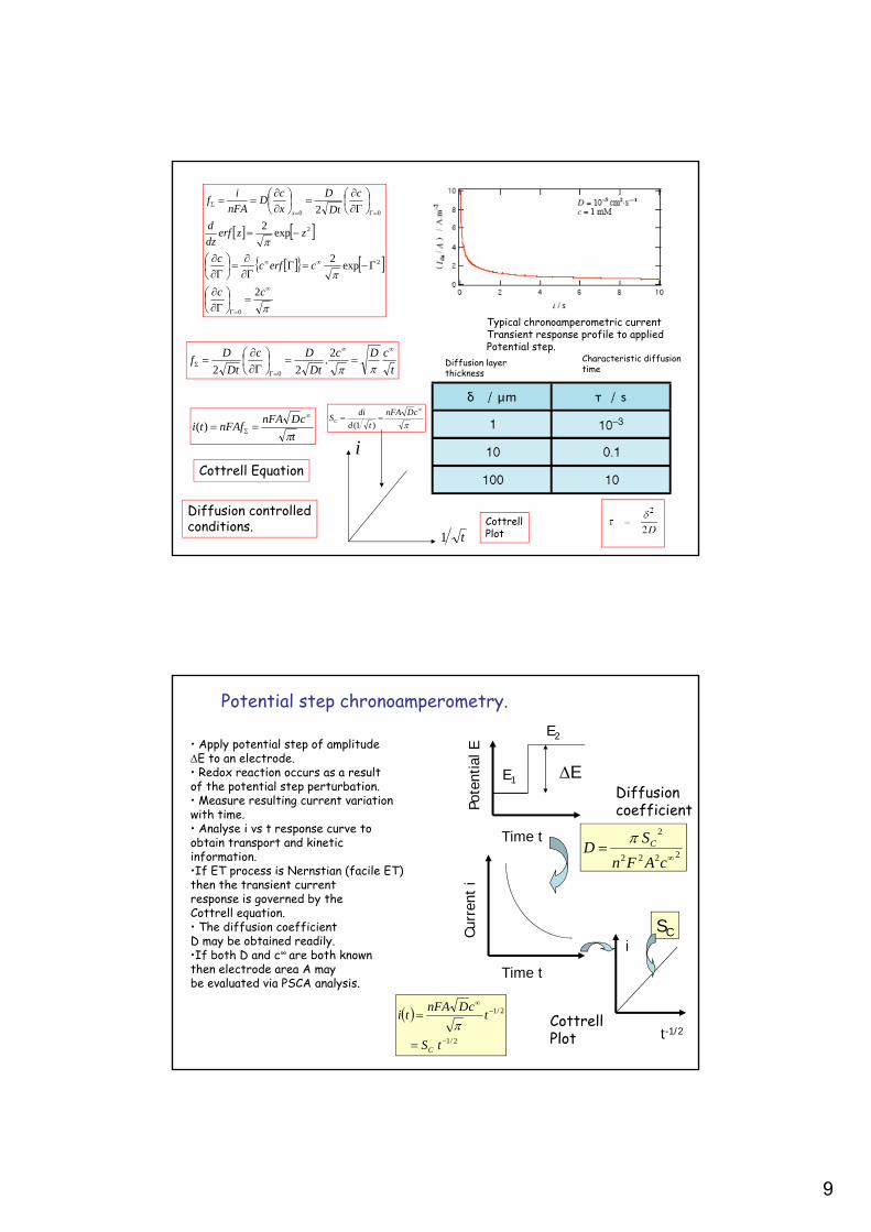
Potential step chronoamperometry : reversible process.We describe the transient electrochemical technique called Potential StepChronoamperometry (PSCA) in which a potential step of magnitude E is applied toan electrode and a Nernstian electrochemical redox transformation occursin response to the potential step perturbation causing a current to flow.We solve the Fick diffusion equation for the problem to derive an expressionfor the transient Faradaic current response as a function of time.

PotentialProfileE = 0.8 V

E

Pulse width (10 s)Expt. duration

Normalised reactant concentrationprofile c(x,t)/c∞.

Transient currentresponse i(t)

Transient coulometricresponse q(t)

CR∞ = 1 mM

D = 1.0 x 10-5cm2s-1

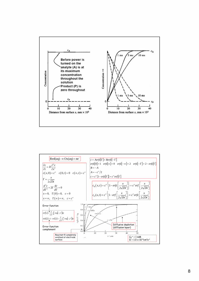
8

2

2

2

2

,0 0, 0 ,

2

2 0

0, 0 0, 0

, ,

c cD

t x

c x c c t c t c

x

Dt

d c dc

d dx c

x c c

erfcerfccc

cA

AB

erfcerfcerfcerfcerfc

BerfcAerfcc

1

2

22010

, 12 2

( , ) 12 2

R

O

x xc x t c erfc c erf

Dt Dt

x xc x t c erf c erfc

Dt Dt

CR∞ = 1 mM

D = 1.0 x 10-5cm2s-1

neOx(aq)Red(aq)

Diffusive depletion(diffusion layer)

Reactant R completelyoxidized at electrodesurface

z

z

dyyzerfzerfc

dyyzerf

2

0

2

exp2

1

exp2

Error function

Error functioncomplement

9

cc

cerfcc

zzerfdz

d

c

Dt

D

x

cD

nFA

if

x

2

exp2

exp2

2

0

2

2

00

t

cDc

Dt

Dc

Dt

Df

2.

22 0

t

cDnFAnFAfti

)(

Cottrell Equation

Diffusion controlledconditions.

Characteristic diffusiontime

Diffusion layerthickness

i

t1

cDnFA

td

diSC

)1(

CottrellPlot

Typical chronoamperometric currentTransient response profile to appliedPotential step.

Potential step chronoamperometry.

• Apply potential step of amplitudeE to an electrode.• Redox reaction occurs as a resultof the potential step perturbation.• Measure resulting current variation with time.• Analyse i vs t response curve toobtain transport and kineticinformation.•If ET process is Nernstian (facile ET)then the transient currentresponse is governed by theCottrell equation.• The diffusion coefficientD may be obtained readily.•If both D and c∞ are both knownthen electrode area A maybe evaluated via PSCA analysis.

2/1

2/1

tS

tcDnFA

ti

C

E2

E1 E

Time t

Pote

ntia

l E

Time t

Curr

ent

i

i

t-1/2

SC

2222

2

cAFn

SD C

Diffusioncoefficient

CottrellPlot

10

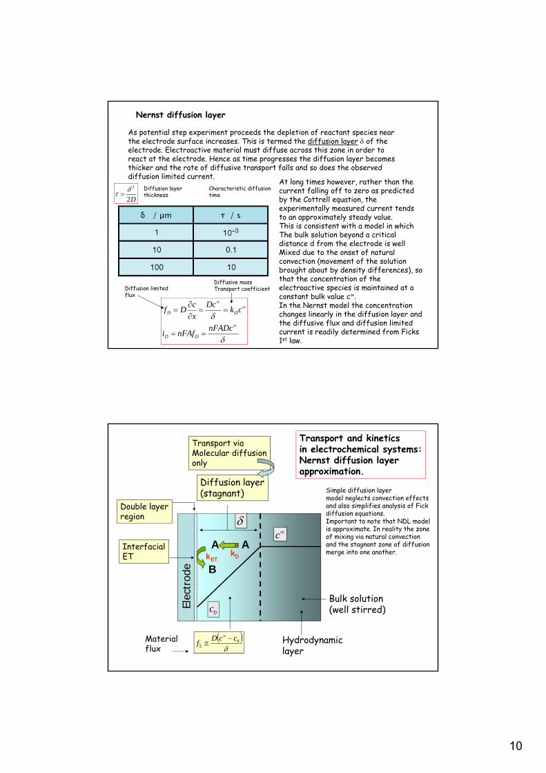
As potential step experiment proceeds the depletion of reactant species nearthe electrode surface increases. This is termed the diffusion layer of the electrode. Electroactive material must diffuse across this zone in order to react at the electrode. Hence as time progresses the diffusion layer becomesthicker and the rate of diffusive transport falls and so does the observeddiffusion limited current.

Nernst diffusion layer

Diffusion layerthickness

Characteristic diffusiontime

D2

2

At long times however, rather than thecurrent falling off to zero as predictedby the Cottrell equation, the experimentally measured current tends to an approximately steady value.This is consistent with a model in whichThe bulk solution beyond a critical distance d from the electrode is wellMixed due to the onset of natural convection (movement of the solution brought about by density differences), so that the concentration of the electroactive species is maintained at a constant bulk value c∞. In the Nernst model the concentration changes linearly in the diffusion layer and the diffusive flux and diffusion limited current is readily determined from Ficks 1st law.

nFADcnFAfi

ckDc

x

cDf

DD

DD

Diffusive massTransport coefficientDiffusion limited

flux

0c

c

Diffusion layer(stagnant)

Bulk solution(well stirred)

0ccDf

Materialflux

Elec

trod

e

Transport viaMolecular diffusiononly

Double layerregion

Hydrodynamiclayer

A

B

AkDkET

Transport and kineticsin electrochemical systems:Nernst diffusion layerapproximation.

InterfacialET

Simple diffusion layermodel neglects convection effectsand also simplifies analysis of Fickdiffusion equations.Important to note that NDL modelis approximate. In reality the zoneof mixing via natural convectionand the stagnant zone of diffusionmerge into one another.

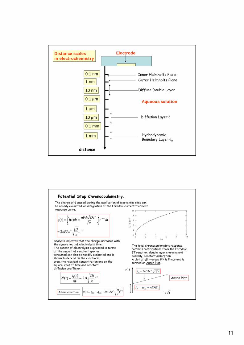
11

0.1 nm

1 nm

10 nm

0.1 m

1 m

10 m

0.1 mm

1 mm

Inner Helmholtz PlaneOuter Helmholtz Plane

Diffuse Double Layer

Diffusion Layer

HydrodynamicBoundary Layer 0

Electrode

Aqueous solution

distance

Distance scalesin electrochemistry

Potential Step Chronocoulometry.The charge q(t) passed during the application of a potential step canbe readily evaluated via integration of the Faradaic current transientresponse curve.

1/ 2

0 0

1/ 2

( ) ( )

2

t tnFA Dcq t i t dt t dt

DnFAc t

Analysis indicates that the charge increases with the square root of electrolysis time.The extent of electrolysis expressed in terms of the amount of reactant speciesconsumed can also be readily evaluated and is shown to depend on the electrodearea, the reactant concentration and on the square root of time and reactant diffusion coefficient.

cDt

AnF

tqtN

2

)()(

The total chronocoulometric responsecontains contributions from the FaradaicET reaction, double layer charging andpossibly, reactant adsorption.A plot of q(t) versus t1/2 is linear and istermed an Anson Plot.

)(tq

t

DnFAcSA 2

nFAqI DLA2/12)( t

DnFAcqqtq adsDL

Anson Plot

Anson equation

12

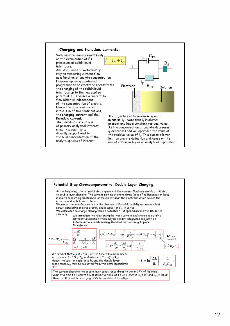
Charging and Faradaic currents.CDL

Electrode RCT

i

iC

iF

RS

Solution

CF iii Voltammetric measurements relyon the examination of ETprocesses at solid/liquidinterfaces.Analytical uses of voltammetryrely on measuring current flowas a function of analyte concentration.However applying a potentialprogramme to an electrode necessitatesthe charging of the solid/liquidinterface up to the new appliedpotential. This causes a current toflow which is independentof the concentration of analyte.Hence the observed currentis the sum of two contributions,the charging current and theFaradaic current.The Faradaic current iF is of primary analytical interestsince this quantity isdirectly proportional tothe bulk concentration of theanalyte species of interest.

The objective is to maximise iF and minimise iC . Note that iC is alwayspresent and has a constant residual value.As the concentration of analyte decreasesiF decreases and will approach the value of the residual value of iC. This places a lowerlimit on analyte detection and hence on theuse of voltammetry as an analytical application.

Potential Step Chronoamperometry: Double Layer Charging.

At the beginning of a potential step experiment the current flowing is mainly attributedto double layer charging. The current flowing at short times (tens of milliseconds or less)is due to supporting electrolyte ion movement near the electrode which causes the interfacial double layer to form.We model the interface region in the absence of Faradaic activity as an equivalentcircuit consisting of a resistor RS and a capacitor CDL in series.We calculate the charge flowing when a potential E is applied across this RS series assembly.

DLS C

qiRE

We introduce the relationship between current and charge to obtain a differential equation which may be readily integrated subject to a suitable initial condition using standard methods (e.g. Laplace Transforms).

00

qt

R

E

CR

q

dt

dqdt

dqi

SDLS

t

ECCR

tECtq DL

DLSDLc exp1exp1

DLSCR

RC timeconstant

DLSS

cc CR

t

R

E

dt

dqti exp)(

We predict that a plot of ln ic versus time t should be linearwith a slope S = 1/RS CDL and intercept I = ln(E/RS).Hence the solution resistance RS and the double layercapacitance CDL may be evaluated from this semi-logarithmicplot.

tCRR

Ei

DLSSc

1lnln

The current charging the double layer capacitance drops to 1/e or 37% of its initialvalue at a time t = and to 5% of its initial value at t = 3. Hence if RS = 1Ω and CDL = 20 Fthen t = 20s and DL charging is 95 % complete at t = 60 s.

13

Charging current and Faradaic current contribution can be computed for various transient electrochemical techniques

Potential step technique.

iE

FE

if EEE )(tiF

)(tiC

i

t

F

CF

ii

ii

DLSSC CR

t

R

Ei exp

2/12/1

2/1

t

cnFADiF

Take readingwhen iC is small.

A similar quantitative analysis can be done for other EC methodssuch as cyclic and linear potential sweep voltammetry.

Charging current decays much more rapidlythan Faradaic current.

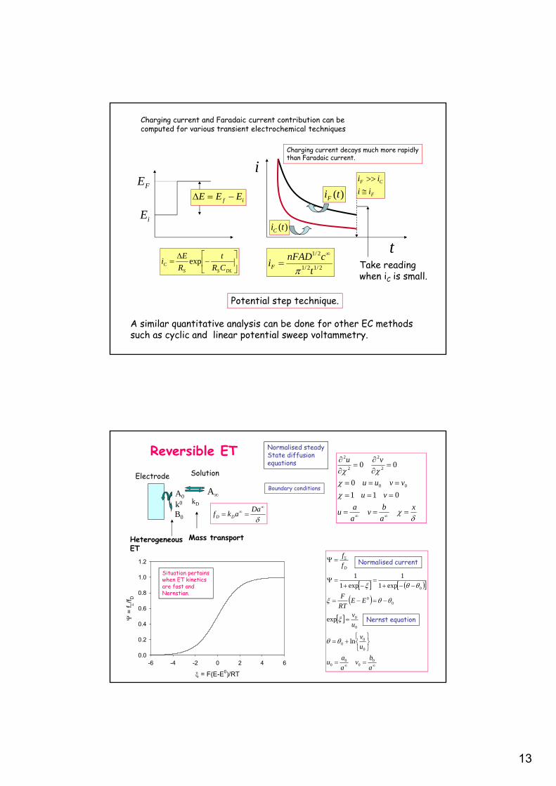
Reversible ET

= F(E-E0)/RT

-6 -4 -2 0 2 4 6

=

f/f D

0.0

0.2

0.4

0.6

0.8

1.0

1.2

a

bv

a

au

u

v

u

v

EERT

F

f

f

D

00

00

0

00

0

0

00

0

ln

exp

exp1

1

exp1

1

x

a

bv

a

au

vu

vvuu

vu

011

0

00

00

2

2

2

2

Normalised current

Nernst equation

Mass transportHeterogeneousET

AA0

B0

kDk0

Electrode Solution

Daakf DD

Normalised steadyState diffusionequations

Boundary conditions

Situation pertainswhen ET kineticsare fast and Nernstian.

14

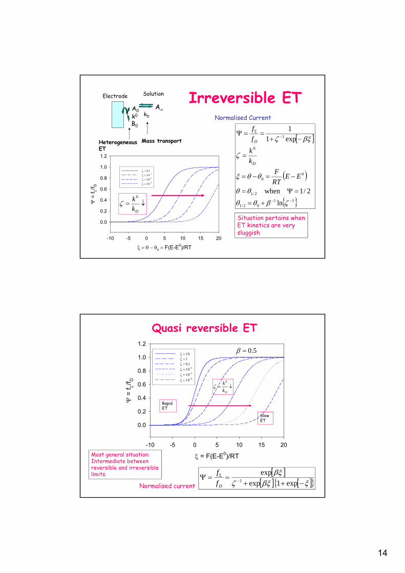
Irreversible ET

F(E-E0)/RT

-10 -5 0 5 10 15 20

=

f/

f D

0.0

0.2

0.4

0.6

0.8

1.0

1.2

1102/1

2/1

00

0

1

ln

2/1when

exp1

1

EERT

F

k

k

f

f

D

DMass transportHeterogeneousET

AA0

B0

kDk0

Electrode Solution

Dk

k 0

Normalised Current

Situation pertains whenET kinetics are verysluggish

= F(E-E0)/RT

-10 -5 0 5 10 15 20

=

f /f

D

0.0

0.2

0.4

0.6

0.8

1.0

1.2

exp1exp

exp1

Df

f

Rapid ET

Slow ET

Dk

k 0

Quasi reversible ET

5.0

Normalised current

Most general situation:Intermediate betweenreversible and irreversiblelimits.

15

= F(E-E0)/RT

-10 -5 0 5 10

-1.5

-1.0

-0.5

0.0

0.5

1.0

1.5

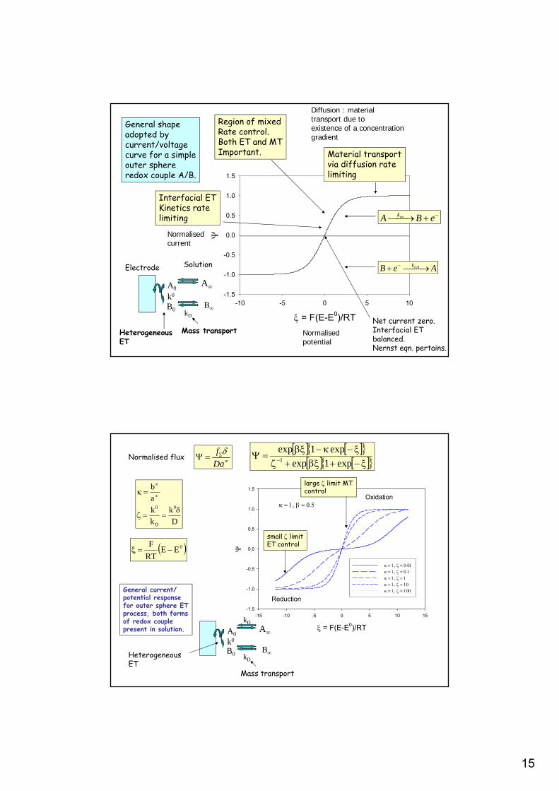
Material transportvia diffusion ratelimiting

Interfacial ETKinetics ratelimiting

Region of mixedRate control.Both ET and MTImportant.

eBA oxk

AeB redk

General shapeadopted bycurrent/voltagecurve for a simpleouter sphereredox couple A/B.

Mass transportHeterogeneousET

AA0

B0B

kD

k0

Electrode Solution

Net current zero.Interfacial ETbalanced.Nernst eqn. pertains.

Diffusion : materialtransport due toexistence of a concentrationgradient

Normalisedpotential

Normalisedcurrent

= F(E-E0)/RT

-15 -10 -5 0 5 10 15

-1.5

-1.0

-0.5

0.0

0.5

1.0

1.5

Oxidation

Reduction

exp1exp

exp1exp1

small limitET control

large limit MTcontrol

D

k

k

k

a

b

0

D

0

f

Da

Normalised flux

0EERT

F

General current/potential responsefor outer sphere ETprocess, both formsof redox couplepresent in solution.

kD

HeterogeneousET

AA0

B0B

kD

k0

Mass transport

16

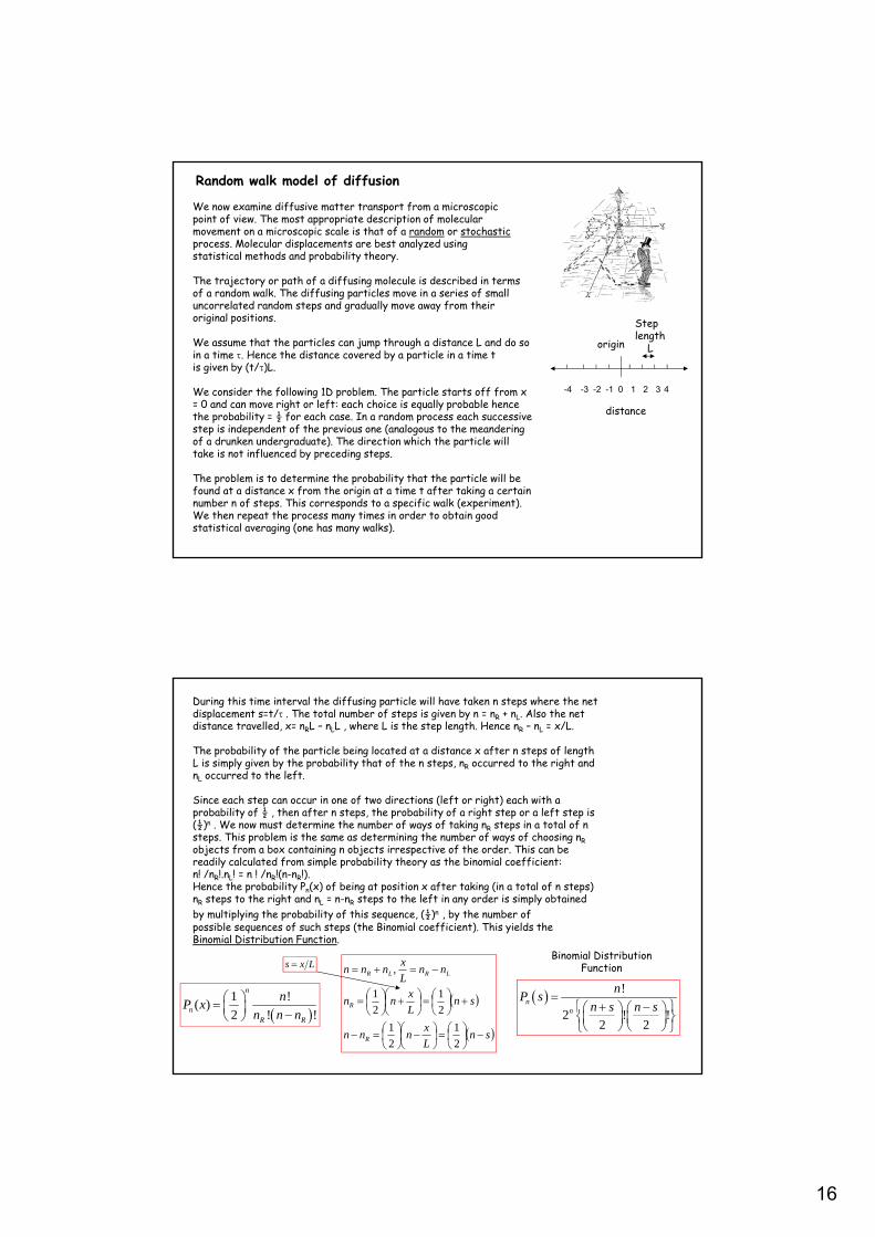
Random walk model of diffusion

We now examine diffusive matter transport from a microscopicpoint of view. The most appropriate description of molecularmovement on a microscopic scale is that of a random or stochastic process. Molecular displacements are best analyzed usingstatistical methods and probability theory.

The trajectory or path of a diffusing molecule is described in terms of a random walk. The diffusing particles move in a series of small uncorrelated random steps and gradually move away from theiroriginal positions.

We assume that the particles can jump through a distance L and do so in a time . Hence the distance covered by a particle in a time tis given by (t/)L.

We consider the following 1D problem. The particle starts off from x = 0 and can move right or left: each choice is equally probable hence the probability = ½ for each case. In a random process each successivestep is independent of the previous one (analogous to the meandering of a drunken undergraduate). The direction which the particle will take is not influenced by preceding steps.

The problem is to determine the probability that the particle will be found at a distance x from the origin at a time t after taking a certain number n of steps. This corresponds to a specific walk (experiment). We then repeat the process many times in order to obtain good statistical averaging (one has many walks).

0 1 2 3 4-1-2-3-4

origin L

distance

Step length

During this time interval the diffusing particle will have taken n steps where the netdisplacement s=t/. The total number of steps is given by n = nR + nL. Also the net distance travelled, x= nRL – nLL , where L is the step length. Hence nR – nL = x/L.

The probability of the particle being located at a distance x after n steps of length L is simply given by the probability that of the n steps, nR occurred to the right and nL occurred to the left.

Since each step can occur in one of two directions (left or right) each with a probability of ½ , then after n steps, the probability of a right step or a left step is (½)n . We now must determine the number of ways of taking nR steps in a total of n steps. This problem is the same as determining the number of ways of choosing nRobjects from a box containing n objects irrespective of the order. This can be readily calculated from simple probability theory as the binomial coefficient: n! /nR!.nL! = n ! /nR!(n-nR!).Hence the probability Pn(x) of being at position x after taking (in a total of n steps) nR steps to the right and nL = n-nR steps to the left in any order is simply obtained by multiplying the probability of this sequence, (½)n , by the number of possible sequences of such steps (the Binomial coefficient). This yields theBinomial Distribution Function.

1 !

( )2 ! !

n

nR R

nP x

n n n

snL

xnnn

snL

xnn

nnL

xnnn

R

R

LRLR

2

1

2

1

2

1

2

1

,

!

2 ! !2 2

nn

nP s

n s n s

Lxs Binomial Distribution

Function

17

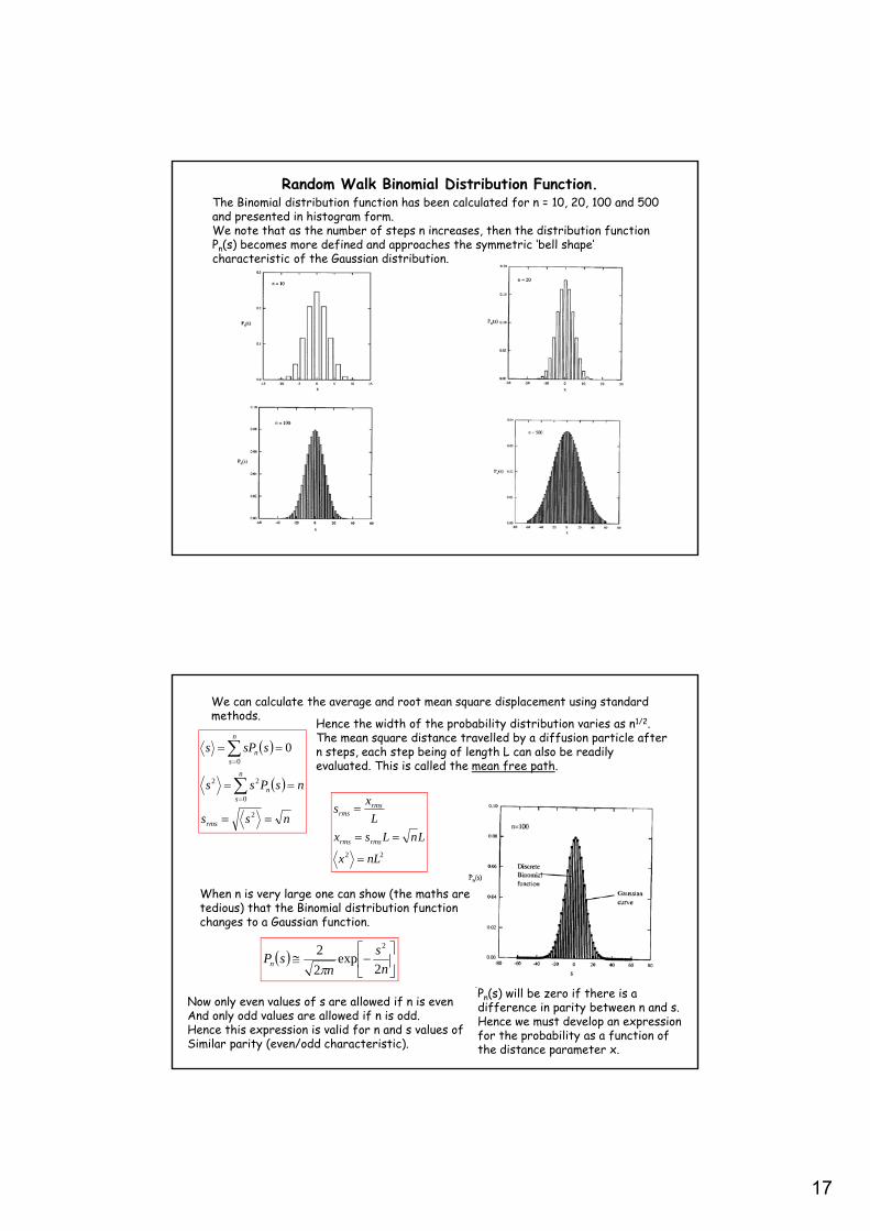
Random Walk Binomial Distribution Function.The Binomial distribution function has been calculated for n = 10, 20, 100 and 500 and presented in histogram form.We note that as the number of steps n increases, then the distribution function Pn(s) becomes more defined and approaches the symmetric ‘bell shape’ characteristic of the Gaussian distribution.

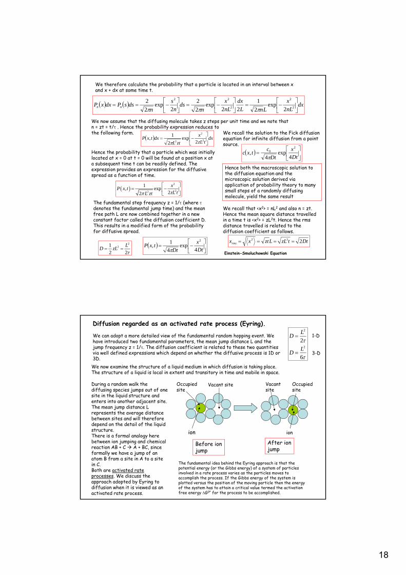
We can calculate the average and root mean square displacement using standard methods.

nss

nsPss

ssPs

rms

n

sn

n

sn

2

0

22

0

0

Hence the width of the probability distribution varies as n1/2.The mean square distance travelled by a diffusion particle after n steps, each step being of length L can also be readily evaluated. This is called the mean free path.

22 nLx

LnLsx

L

xs

rmsrms

rmsrms

When n is very large one can show (the maths are tedious) that the Binomial distribution function changes to a Gaussian function.

n

s

nsPn 2

exp2

2 2

Now only even values of s are allowed if n is evenAnd only odd values are allowed if n is odd.Hence this expression is valid for n and s values ofSimilar parity (even/odd characteristic).

Pn(s) will be zero if there is a difference in parity between n and s.Hence we must develop an expressionfor the probability as a function ofthe distance parameter x.

18

We therefore calculate the probability that a particle is located in an interval between x and x + dx at some time t.

dxnL

x

LnL

dx

nL

x

nds

n

s

ndssPdxxP nn

2

2

2

22

2exp

2

1

22exp

2

2

2exp

2

2

We now assume that the diffusing molecule takes z steps per unit time and we note thatn = zt = t/ . Hence the probability expression reduces tothe following form.

dxtzL

x

ztLdxtxP

2

2

2 2exp

2

1,

Hence the probability that a particle which was initiallylocated at x = 0 at t = 0 will be found at a position x at a subsequent time t can be readily defined. The expression provides an expression for the diffusive spread as a function of time.

2

22

1, exp

22

xP x t

zL tL zt

The fundamental step frequency z = 1/ (where denotes the fundamental jump time) and the mean free path L are now combined together in a new constant factor called the diffusion coefficient D. This results in a modified form of the probability for diffusive spread.

22

1 22 L

zLD

Dt

x

DttxP

4exp

4

1,

2

We recall the solution to the Fick diffusion equation for infinite diffusion from a point source.

Dt

x

Dt

ctxc

4exp

4,

20

Hence both the macroscopic solution to the diffusion equation and the microscopic solution derived via application of probability theory to many small steps of a randomly diffusing molecule, yield the same result

We recall that <x2> = nL2 and also n = zt.Hence the mean square distance travelledin a time t is <x2> = zL2t. Hence the rmsdistance travelled is related to thediffusion coefficient as follows.

DttzLLztxxrms 222

Einstein-Smoluchowski Equation

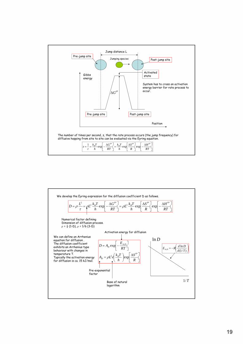
Diffusion regarded as an activated rate process (Eyring).

We can adopt a more detailed view of the fundamental random hopping event. We have introduced two fundamental parameters, the mean jump distance L and the jump frequency z = 1/. The diffusion coefficient is related to these two quantities via well defined expressions which depend on whether the diffusive process is 1D or 3D.

6

22

2

LD

LD

1-D

3-D

ion

Vacant siteOccupiedsite

Vacantsite

Occupiedsite

ion

Before ionjump

After ionjump

We now examine the structure of a liquid medium in which diffusion is taking place.The structure of a liquid is local in extent and transitory in time and mobile in space.

During a random walk the diffusing species jumps out of one site in the liquid structure and enters into another adjacent site.The mean jump distance L represents the average distance between sites and will therefore depend on the detail of the liquid structure.There is a formal analogy here between ion jumping and chemical reaction AB + C A + BC, since formally we have a jump of an atom B from a site in A to a site in C.Both are activated rate processes. We discuss the approach adopted by Eyring to diffusion when it is viewed as an activated rate process.

The fundamental idea behind the Eyring approach is that the potential energy (or the Gibbs energy) of a system of particles involved in a rate process varies as the particles moves to accomplish the process. If the Gibbs energy of the system is plotted versus the position of the moving particle then the energy of the system has to attain a critical value termed the activation free energy G0* for the process to be accomplished.

19

Pre-jump site Post-jump site

Post-jump sitePre-jump site

Jump distance L

Jumping species

Position

Gibbs energy

*0G

Activatedstate

System has to cross an activation energy barrier for rate process to occur.

The number of times per second, z, that the rate process occurs (the jump frequency) fordiffusive hopping from site to site can be evaluated via the Eyring equation.

RT

H

R

S

h

Tk

RT

G

h

Tkz BB

*0*0*0

expexpexp1

We develop the Eyring expression for the diffusion coefficient D as follows.

RT

H

R

S

h

TkL

RT

G

h

TkL

LD BB

*0*02

*02

2

expexpexp

Numerical factor definingDimension of diffusion process. = ½ (1-D), = 1/6 (3-D)

We can define an Arrhenius equation for diffusion .The diffusion coefficient exhibits an Arrhenius type behaviour with changes in temperature T.Typically the activation energy for diffusion is ca. 15 kJ/mol.

R

S

h

TkeLA

RT

EAD

BD

DAD

*02

,

exp

exp

Pre-exponential factor

Base of naturallogarithm

Activation energy for diffusion

Dln

T/1

)/1(

ln, Td

DdRE DA

20

Linear sweep and cyclic voltammetry.

• Linear sweep voltammetry (LPSV) and cyclic voltammetry (CV) are the most well known and popular electrochemical technique in use today.

• In both techniques a defined time varying potential ramp is applied to a working electrode causing an interfacial ET reaction to occur. The current flowing from this process is monitored and the resulting plot of current versus applied potential (the voltammogram) is recorded.

• Again the quantitative basis of the method is the solution of the time dependent Fick diffusion equation.

• This initial and boundary value problem cannot be solved totally analytically but the integral equation obtained which describes the voltammetric current response has to be solved numerically.

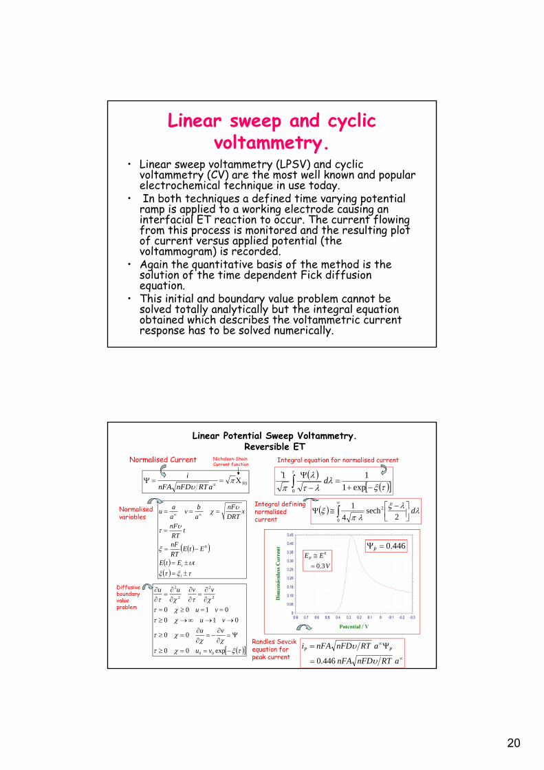
Linear Potential Sweep Voltammetry.Reversible ET

NSaRTnFDnFA

i

exp00

00

010

0100

00

2

2

2

2

vu

vu

vu

vu

vvuu

exp1

11̀

0

d

i

i tEtE

EtERT

nF

tRT

nF

xDRT

nF

a

bv

a

au

0

d

2sech

4

1 2

0

446.0P

aRTnFDnFA

aRTnFDnFAi PP

446.0

Normalised Current

Normalisedvariables

Diffusiveboundaryvalueproblem

Integral equation for normalised current

Integral definingnormalisedcurrent

Randles Sevcikequation forpeak current

Nicholson-ShainCurrent function

V

EEP

3.0

0

21

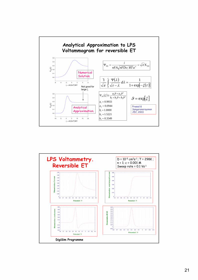
Analytical Approximation to LPS Voltammogram for reversible ET

nF(E-E0)/RT

-10 -5 0 5 10 15 20

N

S(

)

0.0

0.1

0.2

0.3

0.4

0.5

3349.0

5221.1

0000.1

0944.0

9933.0

3

2

1

2

1

2321

221

b

b

b

a

a

bbb

aaNS

NSNSaRTnFDnFA

i

exp1

11̀

0

dnF(E-E0)/RT

-6 -4 -2 0 2 4 6

N

S(

)

0.0

0.1

0.2

0.3

0.4

0.5

exp

Prasad &SangaranarayananJEC, 2003

Not good for large

NumericalSolution.

AnalyticalApproximation.

LPS Voltammetry.Reversible ET

D = 10-5 cm2s-1 ; T = 298K ; n = 1; c = 0.001 MSweep rate = 0.1 Vs-1

DigiSim Programme

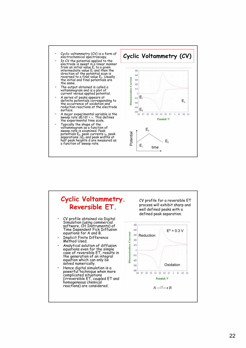
22

Cyclic Voltammetry (CV)• Cyclic voltammetry (CV) is a form of electrochemical spectroscopy.

• In CV the potential applied to the electrode is swept in a linear manner from an initial value Ei to a given intermediate value El, and then the direction of the potential scan is reversed to a final value Ef. Usually the initial and final potentials are the same.

• The output obtained is called a voltammogram and is a plot of current versus applied potential.

• A series of peaks appears at definite potentials corresponding to the occurrence of oxidation and reduction reactions at the electrode surface.

• A major experimental variable is the sweep rate dE/dt = . This defines the experimental time scale.

• Typically the shape of the voltammogram as a function of sweep rate is examined. Peak potentials EP, peak currents iP, peak separations EP and peak widths at half peak heights d are measured as a function of sweep rate. P

oten

tial

timeEi

E

Ef

EiE

Ef

Cyclic Voltammetry.Reversible ET.

• CV profile obtained via Digital Simulation (using commercial software, CH Instruments) of Time Dependent Fick Diffusion equations for A and B.

• Implicit Finite Difference Method Used.

• Analytical solution of diffusion equations even for the simple case of reversible ET, results in the generation of an integral equation which can only be solved numerically.

• Hence digital simulation is a powerful technique when more complicated situations (irreversible ET, coupled ET and homogeneous chemical reactions) are considered. BA e

Reduction

Oxidation

E0 = 0.3 V

CV profile for a reversible ETprocess will exhibit sharp andwell defined peaks with adefined peak separation.

23

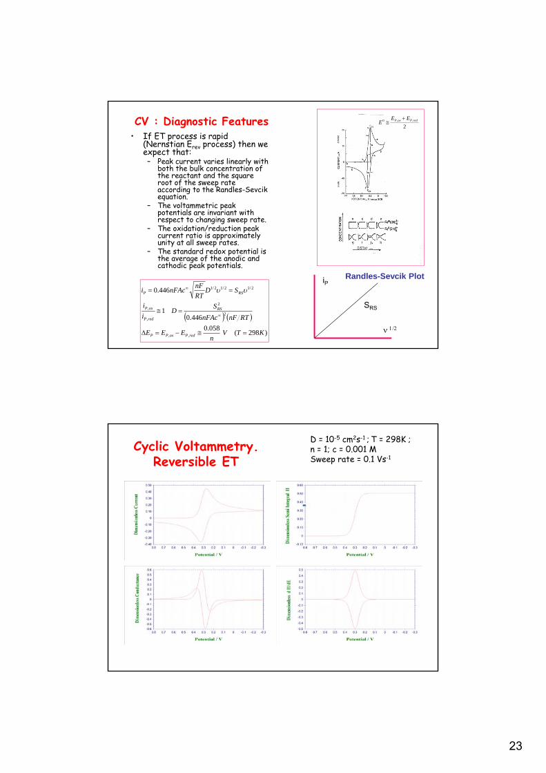
CV : Diagnostic Features• If ET process is rapid

(Nernstian Erev process) then we expect that:– Peak current varies linearly with

both the bulk concentration of the reactant and the square root of the sweep rate according to the Randles-Sevcik equation.

– The voltammetric peak potentials are invariant with respect to changing sweep rate.

– The oxidation/reduction peak current ratio is approximately unity at all sweep rates.

– The standard redox potential is the average of the anodic and cathodic peak potentials.

)298(058.0

446.01

446.0

,,

2

2

,

,

2/12/12/1

KTVn

EEE

RTnFnFAc

SD

i

i

SDRT

nFnFAci

redPoxPP

RS

redP

oxP

RSP

iP

SRS

Randles-Sevcik Plot

2,,0 redPoxP EE

E

Cyclic Voltammetry.Reversible ET

D = 10-5 cm2s-1 ; T = 298K ; n = 1; c = 0.001 MSweep rate = 0.1 Vs-1

24

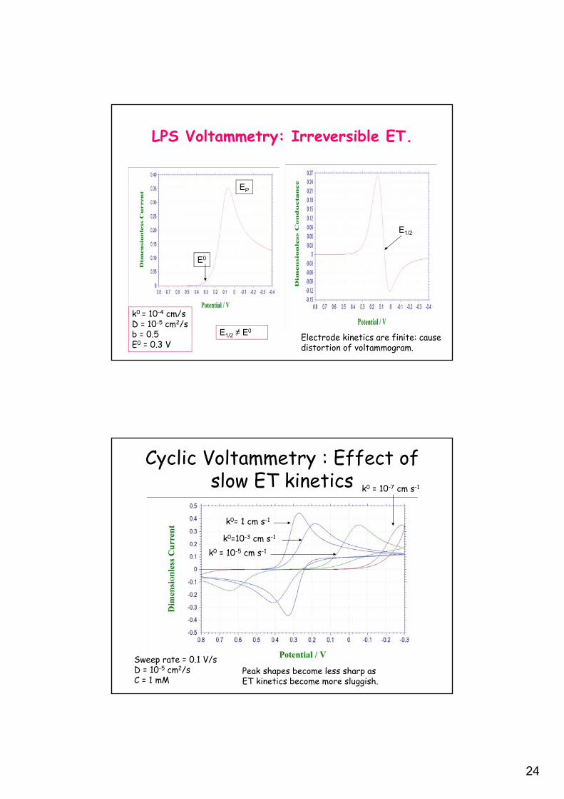
LPS Voltammetry: Irreversible ET.

k0 = 10-4 cm/sD = 10-5 cm2/sb = 0.5E0 = 0.3 V

E1/2

E1/2 ≠ E0

E0

EP

Electrode kinetics are finite: causedistortion of voltammogram.

Cyclic Voltammetry : Effect of slow ET kinetics

k0= 1 cm s-1

k0=10-3 cm s-1

k0 = 10-5 cm s-1

k0 = 10-7 cm s-1

Sweep rate = 0.1 V/sD = 10-5 cm2/sC = 1 mM

Peak shapes become less sharp asET kinetics become more sluggish.

25

N

0.01 0.1 1 10 100

n E

P/m

V

40

60

80

100

120

140

160

180

200

220

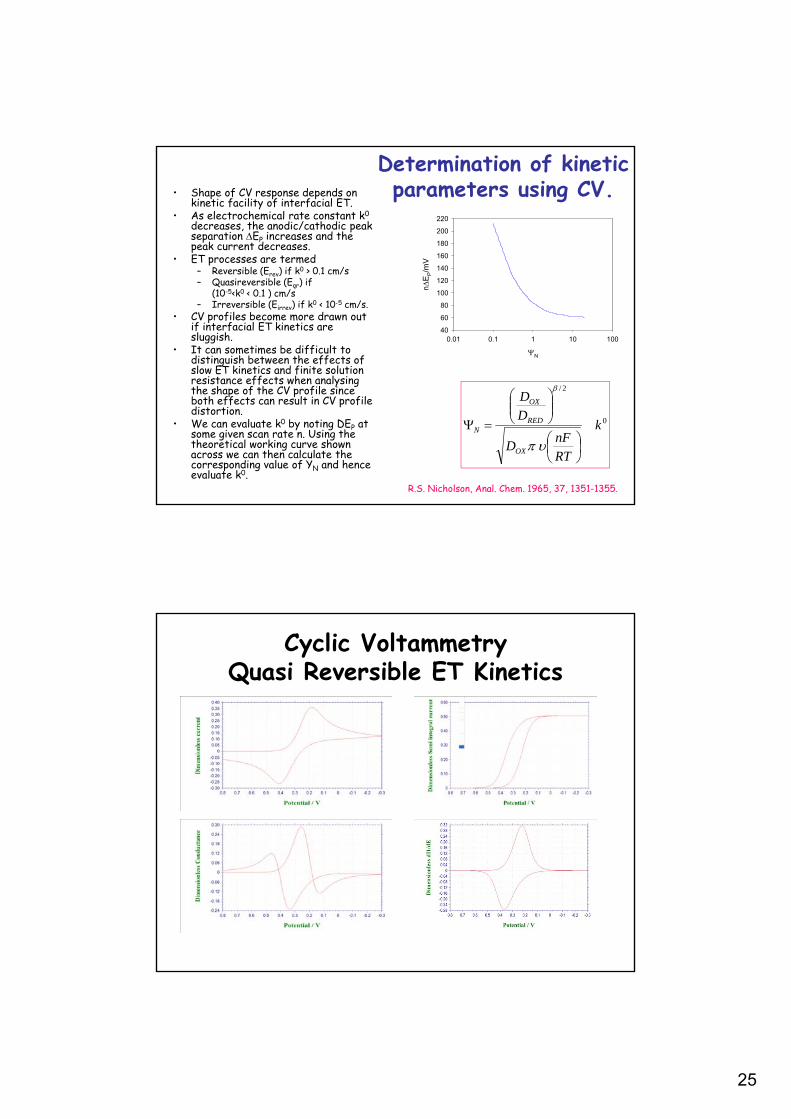
Determination of kinetic parameters using CV.• Shape of CV response depends on

kinetic facility of interfacial ET.• As electrochemical rate constant k0

decreases, the anodic/cathodic peak separation EP increases and the peak current decreases.

• ET processes are termed– Reversible (Erev) if k0 > 0.1 cm/s– Quasireversible (Eqr) if

(10-5<k0 < 0.1 ) cm/s– Irreversible (Eirrev) if k0 < 10-5 cm/s.

• CV profiles become more drawn out if interfacial ET kinetics are sluggish.

• It can sometimes be difficult to distinguish between the effects of slow ET kinetics and finite solution resistance effects when analysing the shape of the CV profile since both effects can result in CV profile distortion.

• We can evaluate k0 by noting DEP at some given scan rate n. Using the theoretical working curve shown across we can then calculate the corresponding value of YN and hence evaluate k0.

0

2/

k

RTnF

D

DD

OX

RED

OX

N

R.S. Nicholson, Anal. Chem. 1965, 37, 1351-1355.

Cyclic VoltammetryQuasi Reversible ET Kinetics

26

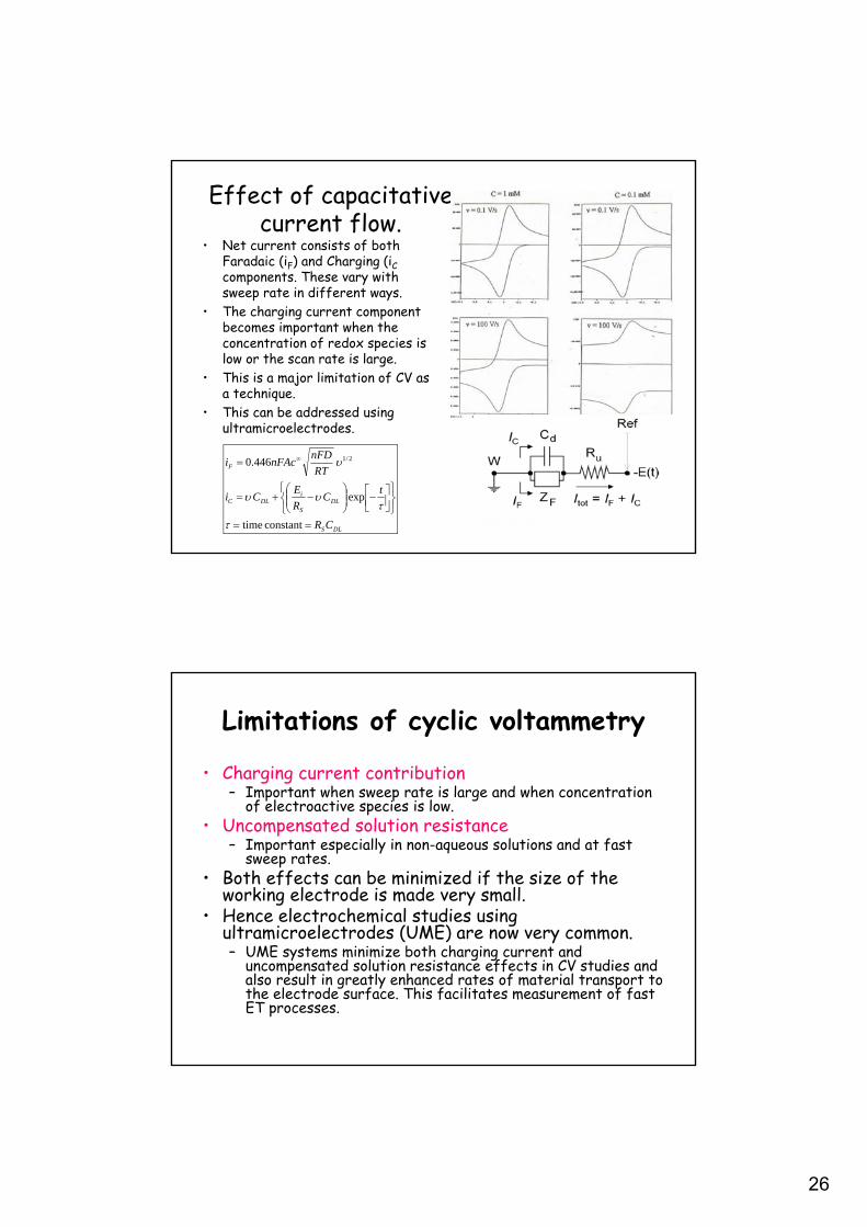
Effect of capacitative current flow.

• Net current consists of both Faradaic (iF) and Charging (iCcomponents. These vary with sweep rate in different ways.

• The charging current component becomes important when the concentration of redox species is low or the scan rate is large.

• This is a major limitation of CV as a technique.

• This can be addressed using ultramicroelectrodes.

DLS

DLS

iDLC

F

CR

tC

R

ECi

RT

nFDnFAci

constant time

exp

446.0 2/1

Limitations of cyclic voltammetry

• Charging current contribution– Important when sweep rate is large and when concentration

of electroactive species is low.• Uncompensated solution resistance

– Important especially in non-aqueous solutions and at fast sweep rates.

• Both effects can be minimized if the size of the working electrode is made very small.

• Hence electrochemical studies using ultramicroelectrodes (UME) are now very common.– UME systems minimize both charging current and

uncompensated solution resistance effects in CV studies and also result in greatly enhanced rates of material transport to the electrode surface. This facilitates measurement of fast ET processes.

27

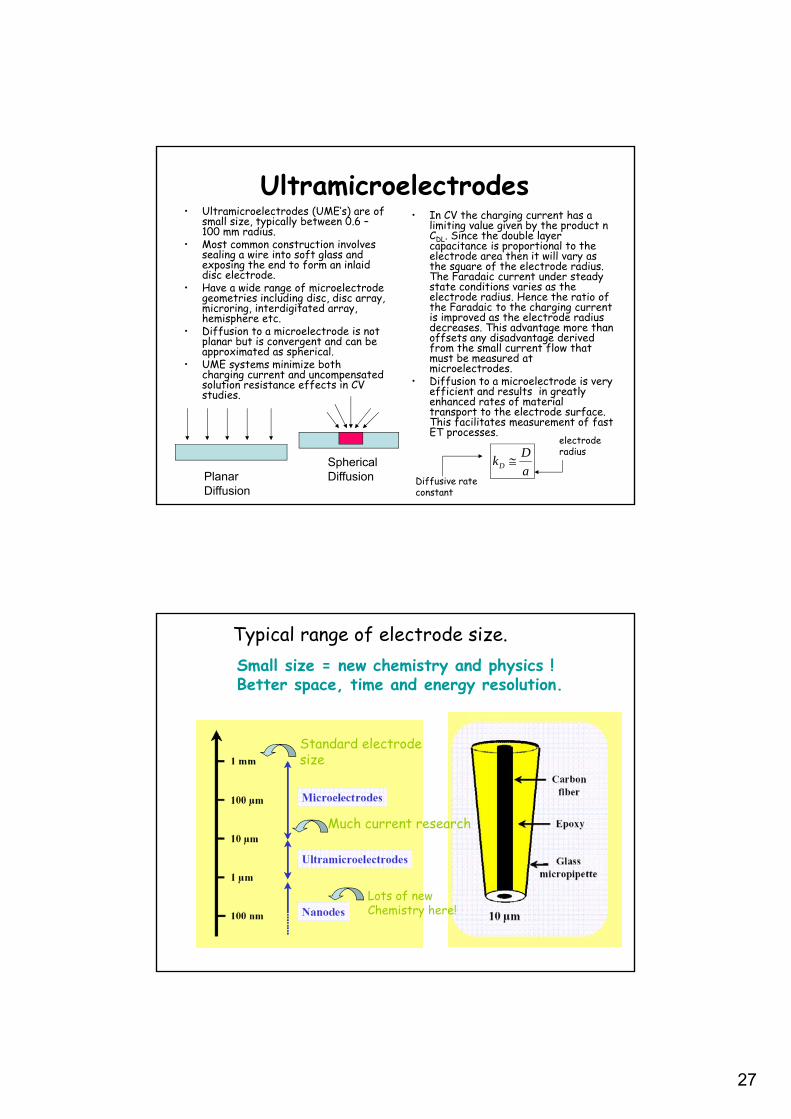
Ultramicroelectrodes• Ultramicroelectrodes (UME’s) are of

small size, typically between 0.6 –100 mm radius.

• Most common construction involves sealing a wire into soft glass and exposing the end to form an inlaid disc electrode.

• Have a wide range of microelectrode geometries including disc, disc array, microring, interdigitated array, hemisphere etc.

• Diffusion to a microelectrode is not planar but is convergent and can be approximated as spherical.

• UME systems minimize both charging current and uncompensated solution resistance effects in CV studies.

• In CV the charging current has a limiting value given by the product n CDL. Since the double layer capacitance is proportional to the electrode area then it will vary as the square of the electrode radius. The Faradaic current under steady state conditions varies as the electrode radius. Hence the ratio of the Faradaic to the charging current is improved as the electrode radius decreases. This advantage more than offsets any disadvantage derived from the small current flow that must be measured at microelectrodes.

• Diffusion to a microelectrode is very efficient and results in greatly enhanced rates of material transport to the electrode surface. This facilitates measurement of fast ET processes.

PlanarDiffusion

SphericalDiffusion a

DkD

electroderadius

Diffusive rateconstant

Typical range of electrode size.

Lots of newChemistry here!

Much current research

Standard electrodesize

Small size = new chemistry and physics !Better space, time and energy resolution.

28

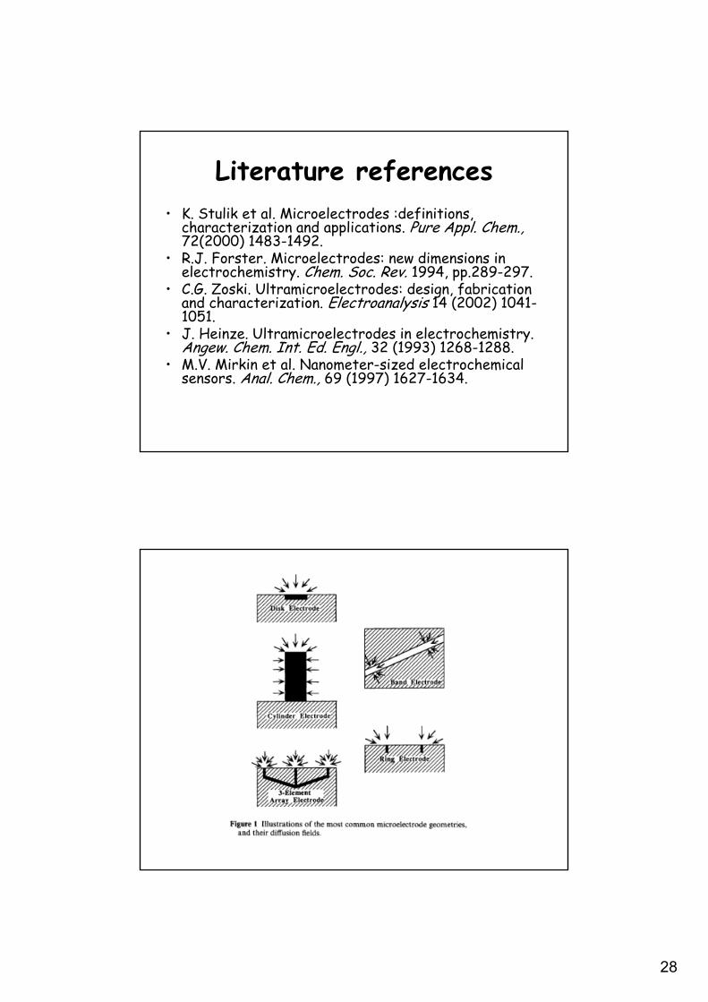
Literature references• K. Stulik et al. Microelectrodes :definitions,

characterization and applications. Pure Appl. Chem.,72(2000) 1483-1492.

• R.J. Forster. Microelectrodes: new dimensions in electrochemistry. Chem. Soc. Rev. 1994, pp.289-297.

• C.G. Zoski. Ultramicroelectrodes: design, fabrication and characterization. Electroanalysis 14 (2002) 1041-1051.

• J. Heinze. Ultramicroelectrodes in electrochemistry. Angew. Chem. Int. Ed. Engl., 32 (1993) 1268-1288.

• M.V. Mirkin et al. Nanometer-sized electrochemical sensors. Anal. Chem., 69 (1997) 1627-1634.

29

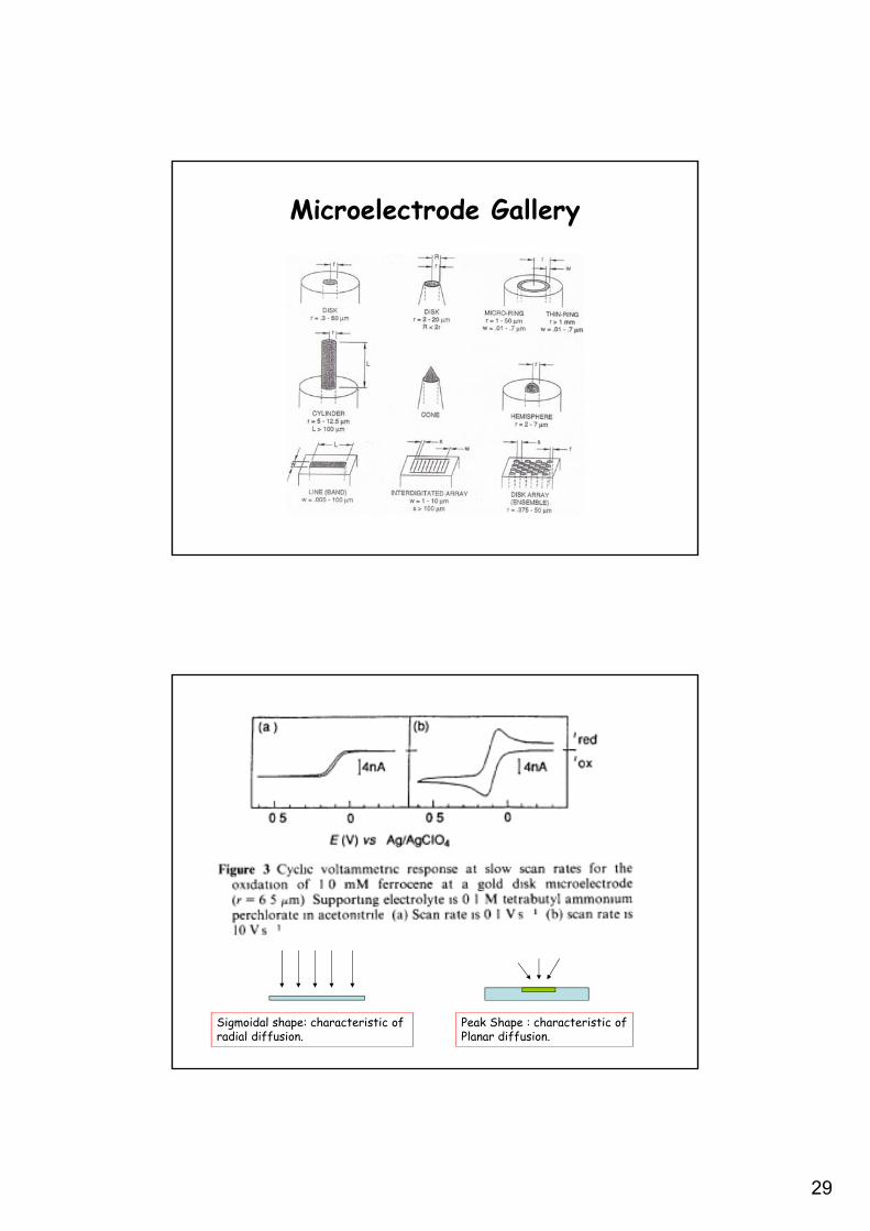
Microelectrode Gallery

Sigmoidal shape: characteristic of radial diffusion.

Peak Shape : characteristic ofPlanar diffusion.

30

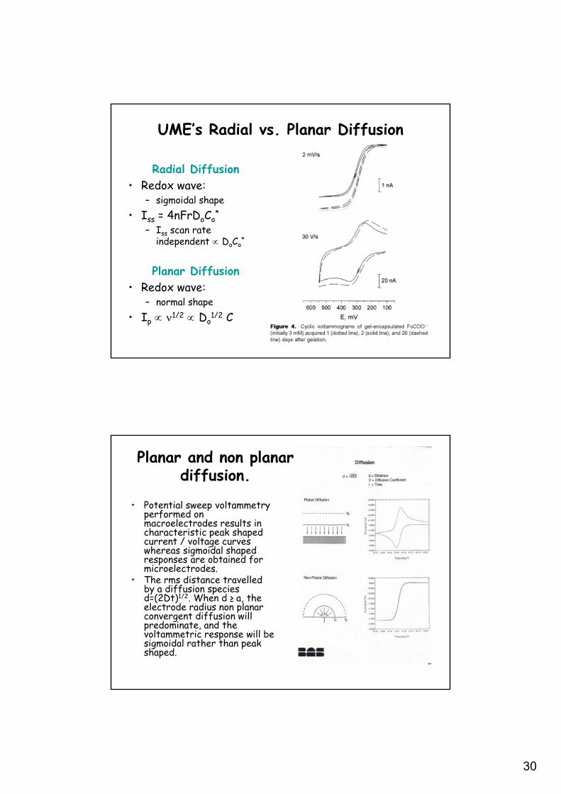
UME’s Radial vs. Planar Diffusion

Radial Diffusion• Redox wave:

– sigmoidal shape• Iss = 4nFrDoCo

*

– Iss scan rate independent DoCo

*

Planar Diffusion• Redox wave:

– normal shape• Ip 1/2 Do

1/2 C

Planar and non planar diffusion.

• Potential sweep voltammetry performed on macroelectrodes results in characteristic peak shaped current / voltage curves whereas sigmoidal shaped responses are obtained for microelectrodes.

• The rms distance travelled by a diffusion species d=(2Dt)1/2. When d ≥ a, the electrode radius non planar convergent diffusion will predominate, and the voltammetric response will be sigmoidal rather than peak shaped.

31

r

c

rr

cD

t

c 22

2

anFDci

anFDci

D

D

2

4

2

2

2

2 1

z

c

r

c

rr

cD

t

canFDciD

4

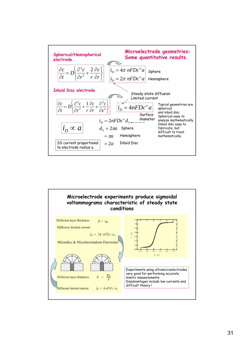
Spherical/Hemispherical electrode

Inlaid Disc electrode

Sphere

Hemisphere

a

a

ad

dnFDci

S

SD

2

2

2

Sphere

Hemisphere

Inlaid Disc

Surfacediameter

Steady state diffusionLimited current

aiD

SS current proportionalto electrode radius a.

Typical geometries are sphericaland inlaid disc.Spherical easy to analyze mathematically.Inlaid disc easy tofabricate, butdifficult to treat mathematically.

Microelectrode geometries:Some quantitative results.

Microelectrode experiments produce sigmoidal voltammograms characteristic of steady state

conditions

Experiments using ultramicroelectrodesvery good for performing accuratekinetic measurements.Disadvantages include low currents anddifficult theory !

32

2aXX

AC

HHDL

anFDciF 4

2aX

CiH

DLC

a

cK

aX

anFDc

i

i

HC

F

2

4

HnFDX

K4

Helmholtz layerthickness

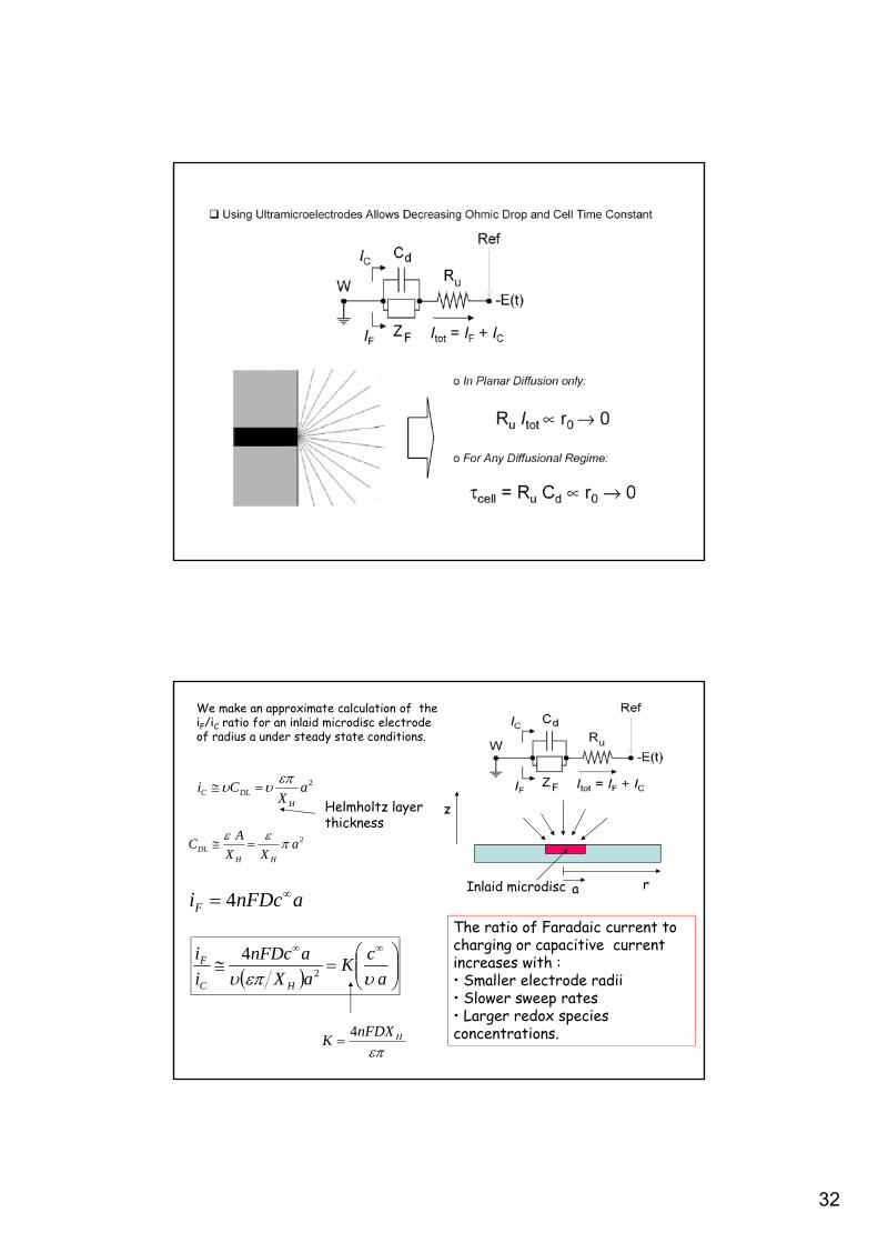
The ratio of Faradaic current to charging or capacitive current increases with :• Smaller electrode radii• Slower sweep rates• Larger redox species concentrations.

We make an approximate calculation of the iF/iC ratio for an inlaid microdisc electrode of radius a under steady state conditions.

Inlaid microdisc a r

z

33

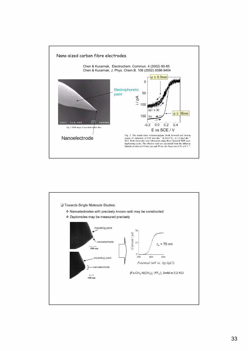
Nano-sized carbon fibre electrodes.

Chen & Kucernak, Electrochem. Commun. 4 (2002) 80-85Chen & Kucernak, J. Phys. Chem.B. 106 (2002) 9396-9404

Nanoelectrode

Electrophoreticpaint

nma 38

nma 9.0

34

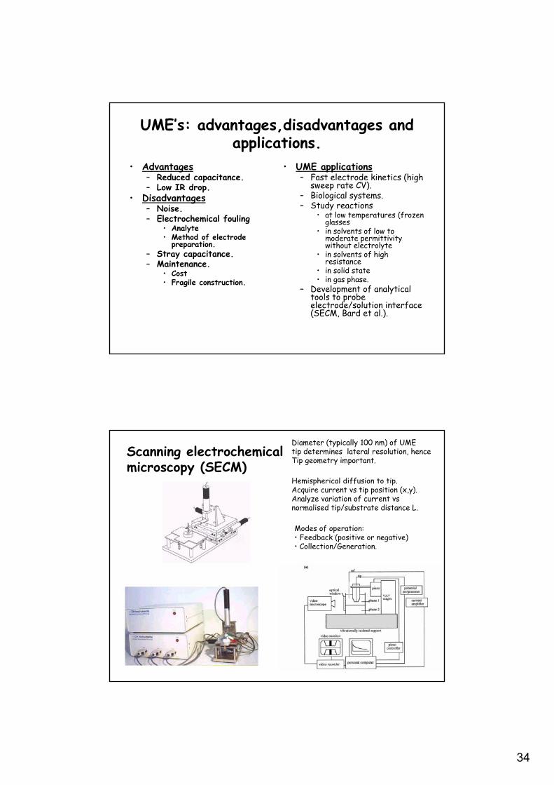
UME’s: advantages,disadvantages and applications.

• Advantages– Reduced capacitance.– Low IR drop.

• Disadvantages– Noise.– Electrochemical fouling

• Analyte• Method of electrode

preparation.– Stray capacitance.– Maintenance.

• Cost• Fragile construction.

• UME applications– Fast electrode kinetics (high

sweep rate CV).– Biological systems.– Study reactions

• at low temperatures (frozen glasses

• in solvents of low to moderate permittivity without electrolyte

• in solvents of high resistance

• in solid state• in gas phase.

– Development of analytical tools to probe electrode/solution interface (SECM, Bard et al.).

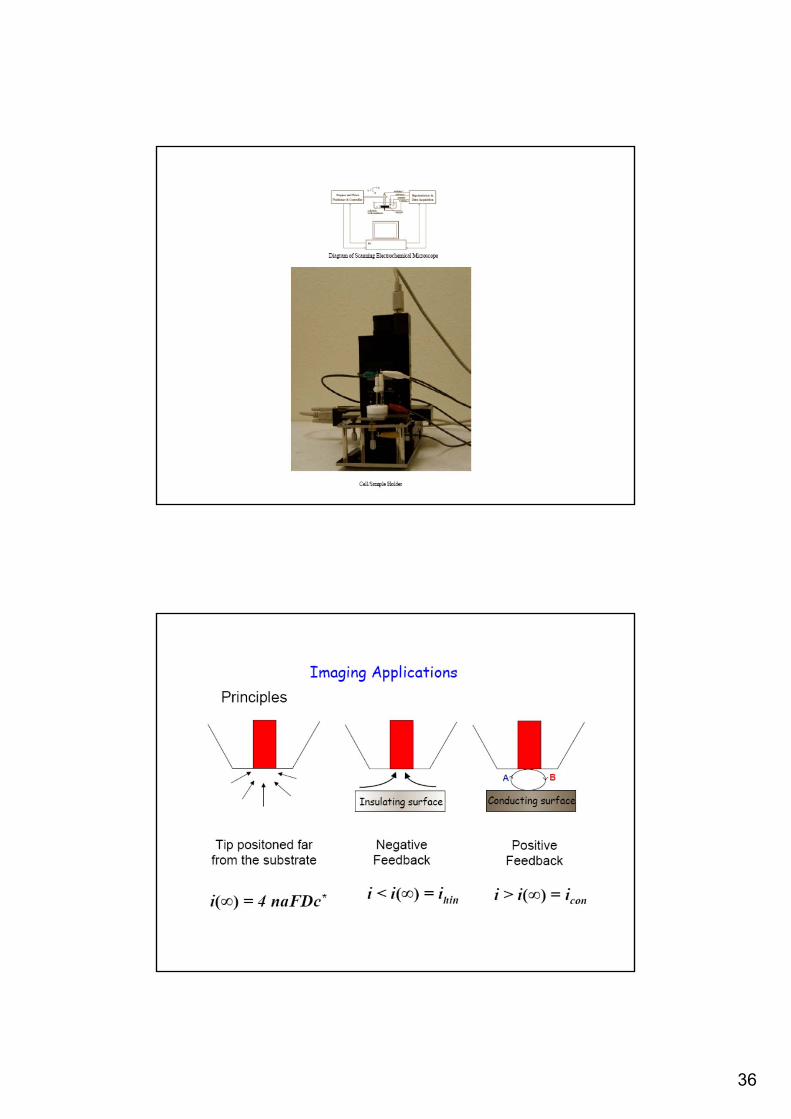
Scanning electrochemical microscopy (SECM)

Diameter (typically 100 nm) of UME tip determines lateral resolution, henceTip geometry important.

Modes of operation:• Feedback (positive or negative)• Collection/Generation.

Hemispherical diffusion to tip.Acquire current vs tip position (x,y).Analyze variation of current vs normalised tip/substrate distance L.

35

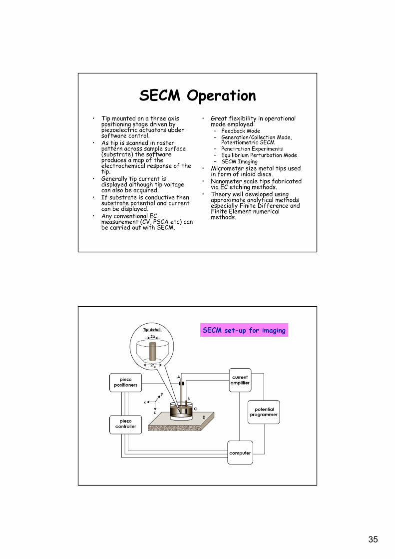
SECM Operation• Tip mounted on a three axis

positioning stage driven by piezoelectric actuators ubder software control.

• As tip is scanned in raster pattern across sample surface (substrate) the software produces a map of the electrochemical response of the tip.

• Generally tip current is displayed although tip voltage can also be acquired.

• If substrate is conductive then substrate potential and current can be displayed.

• Any conventional EC measurement (CV, PSCA etc) can be carried out with SECM.

• Great flexibility in operational mode employed:– Feedback Mode– Generation/Collection Mode,

Potentiometric SECM– Penetration Experiments– Equilibrium Perturbation Mode– SECM Imaging

• Micrometer size metal tips used in form of inlaid discs.

• Nanometer scale tips fabricated via EC etching methods.

• Theory well developed using approximate analytical methods especially Finite Difference and Finite Element numerical methods.

36

37

Feedback Modes

• For an oxidizable redox mediator A the process occuring at the tip during a feedback experiment is A –ne- B. Now if ET is poised sufficiently positive then the rate of reaction is diffusion controlled. For large L and if an inlaid disc is used then iT∞ = 4nFDc∞a.

• When L is smaller the product species B can diffuse to the substrate where it can be reduced back to A via B + ne- A.

• This reaction produces an additional flux of A to the tip and hence an increase in tip current and so iT > iT∞. When this reaction is also diffusion limited the tip current reaches a maximum value.

• This phenomenon is termed positive feedback.

• As tip-substrate distance d decreases, iT increases without limit.

• Negative feedback is the terminology used for situations where the product B does not react at the substrate surface since it may be insulating or the A/B reaction may be kinetically irreversible.

• In the feedback mode the tip potential is set to a value at which a particular species in the solution such as a redox mediator is consumed.

• Feedback is the term used to indicate that the measured tip current is influenced by the rate at which the mediator is regenerated at the substrate.

• The substrate may also be subjected to an independent bias and serve as a second working electrode, although it is not necessary that the substrate be another electrode or even be conductive.

• The feedback effect is sensitive to the tip-substrate separation d and this distance can be expressed in units of tip radius as L = d/a.

• At large values of normalised distance L the tip diffusion layer is not effected by the substrate and is independent of L.

• An inlaid microdisc is often used since this tip surface is parallel to the substrate surface and maximizes the feedback effect. Conical electrodes of the type used in STM produce smaller feedback effects than the disc.

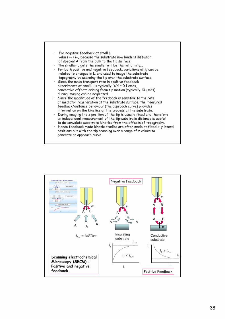
38

• For negative feedback at small L values iT < iT∞ because the substrate now hinders diffusionof species A from the bulk to the tip surface.

• The smaller L gets the smaller will be the ratio iT/iT∞.• For both positive and negative feedback, variations of iT can be

related to changes in L, and used to image the substrate topography by scanning the tip over the substrate surface.

• Since the mass transport rate in positive feedbackexperiments at small L is typically D/d ~ 0.1 cm/s,convective effects arising from tip motion (typically 10 m/s)during imaging can be neglected.

• Since the magnitude of the feedback is sensitive to the rateof mediator regeneration at the substrate surface, the measuredfeedback/distance behaviour (the approach curve) providesinformation on the kinetics of the process at the substrate.

• During imaging the z position of the tip is usually fixed and thereforean independent measurement of the tip-substrate distance is usefulto de-convolute substrate kinetics from the effects of topography.

• Hence feedback mode kinetic studies are often made at fixed x-y lateral positions but with the tip scanning over a range of z values togenerate an approach curve.

A B

A A

Insulatingsubstrate

e-

L

,TiTi

A B

BA

e-

e-

Conductivesubstrate

Ti

,Ti

L

A B

A AA

e-

nFDcaiT 4,

,TT ii ,TT ii

Scanning electrochemicalMicroscopy (SECM) :Positive and negativefeedback.

Negative Feedback

Positive Feedback

39

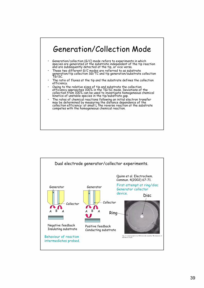
Generation/Collection Mode• Generation/collection (G/C) mode refers to experiments in which

species are generated at the substrate independent of the tip reaction and are subsequently detected at the tip, or vice versa.

• These two different G/C modes are referred to as substrate generation/tip collection SG/TC and tip generation/substrate collection TG/SC.

• The ratio of fluxes at the tip and the substrate defines the collection efficiency.

• Owing to the relative sizes of tip and substrate the collection efficiency approaches 100% in the TG/SC mode. Deviations of the collection from 100% can be used to investigate homogeneous chemical kinetics of unstable species in the tip/substrate gap.

• The rates of chemical reactions following an initial electron transfer may be determined by measuring the distance dependence of the collection efficiency: at small L the reverse reaction at the substrate competes with the homogeneous chemical reaction.

A B A A B A

Negative feedbackInsulating substrate

Positive feedbackConducting substrate

Generator

Collector

Generator

Collector

Dual electrode generator/collector experiments.

First attempt at ring/discGenerator collectordevice. Disc

Ring

Behaviour of reactionintermediates probed.

Quinn et al. Electrochem.Commun. 4(2002) 67-71.