Embed Size (px)
Citation preview

US Department of the Interior National Park Service
National Center for Preservation Technology and Training
Publication No. 1998-1l
Physical and Chemical Processes of Soiling and Washoff at the Cathedral of Learning.
Progress Report for the National Park Service
U.S. Department of the interior Cooperative Agreement 1443CA001960035
with Carnegie Mellon University
Report Authors Graduate Students: Vicken Etycmezian
Ross Strader
Faculty: Cliff Davidson Susan Finger
Undergraduate Students: Stephannic Behrens Thomas Curry Ivan Locke Preshanth Mekala John Murray Karen Pinkston Warinthorn Songkasiri Jiyoung Lee
Department of Civil and Environmental Engineering Carnegie Mellon University
Pittsburgh, PA 5213
November 1997
Funding for this report was provided by the National Park Service’s National Center for Preservation Technology and Training, Natchitoches, Louisiana. NCPTT promotes and enhances the preservation of prehistoric and
historic resources in the United States for present and future generations through the advancement and dissemination of preservation technology and training.
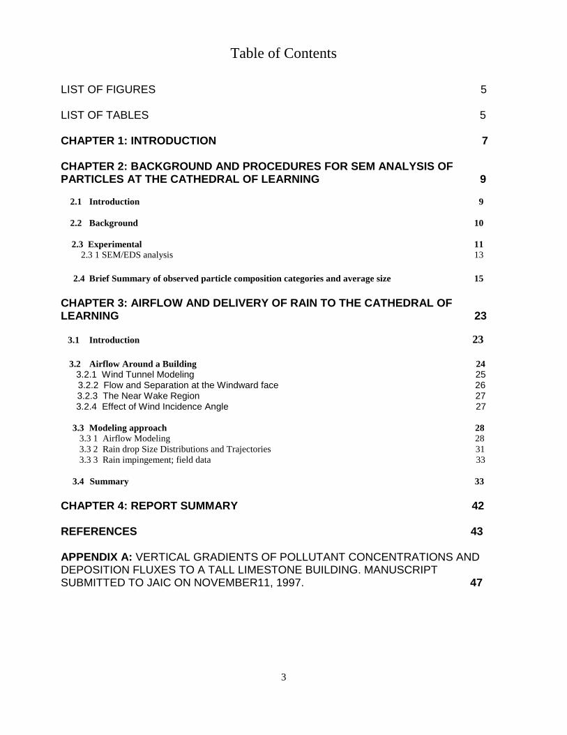
Table of Contents
LIST OF FIGURES 5 LIST OF TABLES 5 CHAPTER 1: INTRODUCTION 7 CHAPTER 2: BACKGROUND AND PROCEDURES FOR SEM ANALYSIS OF PARTICLES AT THE CATHEDRAL OF LEARNING 9 2.1 Introduction 9 2.2 Background 10
2.3 Experimental 11 2.3 1 SEM/EDS analysis 13
2.4 Brief Summary of observed particle composition categories and average size 15 CHAPTER 3: AIRFLOW AND DELIVERY OF RAIN TO THE CATHEDRAL OF LEARNING 23 3.1 Introduction 23 3.2 Airflow Around a Building 24 3.2.1 Wind Tunnel Modeling 25 3.2.2 Flow and Separation at the Windward face 26 3.2.3 The Near Wake Region 27 3.2.4 Effect of Wind Incidence Angle 27 3.3 Modeling approach 28 3.3 1 Airflow Modeling 28 3.3 2 Rain drop Size Distributions and Trajectories 31 3.3 3 Rain impingement; field data 33 3.4 Summary 33 CHAPTER 4: REPORT SUMMARY 42 REFERENCES 43 APPENDIX A: VERTICAL GRADIENTS OF POLLUTANT CONCENTRATIONS AND DEPOSITION FLUXES TO A TALL LIMESTONE BUILDING. MANUSCRIPT SUBMITTED TO JAIC ON NOVEMBER11, 1997. 47
3

LIST OF FIGURES Figure 2 1. Volumetric Displacement Device………………………………………………………….………….18 Figure 2.2 Sampling Locations at the Cathedral of Learning……………………………………………………..19 Figure 2.3. Surrogate Vertical Surfaces for Particle Deposition…………………………………………..………20 Figure 2 4. Schematic of Scanning Electron Microscope…………………………………………………………21 Figure 2.5. Scanning Electron Micrograph and Emission Spectrum for a Predominantly Aluminum Silicate
Particle……………………………………………………………………………..……………………….22 Figure 3 1. Model of Flow Near a Sharp-Edged Three-Dimensional Building in a Deep Boundary Layer. Hosker
(1984)………………………………………………………………………………………………………….………….35 Figure 3.2. Surface Pressure Coefficient on a Cube in a Wind Tunnel. Cas/ro and Robins (1977)……...…………36 Figure 3.3. Example of Computational Grid System for a Cube in a Boundary Layer. Zhou and Stathopoulos
(1996)………………………………………………………………………………………………………..…………….37 Figure 3.4 Example Profiles of Incident Flow Boundary Conditions Zhou and Stathopoulos (1996)…..………....38 Figure 3.5 Computed Shapes of Rain drops of Various Equivalent Diameters Beard and C/wang (1987)..………39 Figure 3.6. Equilibrium Drop Size Distribution as a Function of Drop Diameter. Brown and Whittlesey 1992).…40 Figure 3.7 Schematic of a Disdrometer. Loffler-Mang et al 1996…………………………………………….…………..41 LIST OF TABLES Table 2.1 Sampling Schedule at the Cathedral of Learning………………………………………………………….17
5

CHAPTER 1: INTRODUCTION
Sensitive building materials such as calcareous stone are subject to accelerated deterioration by several agents.
These may be physical processes such as freeze-thaw cycles, chemical processes such as reaction with sulfur dioxide
gas, or biological processes such as attack by microorganisms. We are now beginning to understand some of these
processes though our knowledge is very limited.
This project is oriented toward obtaining an improved understanding of pathways for air pollution damage to
limestone buildings. In particular, we have been studying some of these pathways at the Cathedral of Learning, a 42-
story limestone building on the University of Pittsburgh campus in Pittsburgh, Pennsylvania. Although the focus has
been on this building, the larger goal of this project is to extend experimental and modeling results to other historical
buildings in need of preservation. Such information can help conservators who are deciding on a best course of action
for a deteriorating building. e.g. cleaning, consolidation, or treatment.
Continuing studies within the Cathedral of Learning project can be classified into three Phases. Phase I consists
of on-site measurements of atmospheric pollutant concentrations and deposition. In Phase II. a computer program is
used to model the airflow around the Cathedral. Model results can be used to study mixing in the vicinity of the
Cathedral or as input parameters for later modeling efforts. Finally. Phase III includes development and testing of
mathematical models that describe physical events such as surface rain washing and mass transfer of atmospheric
pollutants to building surfaces. In addition to the three Phases, several long-term undergraduate projects are in progress.
These include developing a computer database for storage of project data, photo-documenting current soiling patterns on
the Cathedral. measuring vertical wind speeds near the walls of the Cathedral, and developing devices for measurement
of rain flux to the building walls.
This report summarizes the work conducted on the Cathedral of Learning project during the period
November 15, 1996 to November 15. 1997. Each of the three Phases described above is represented in the report.
Chapter 2 contains experimental procedures and a very brief summary of results for two types of samples that were
obtained at the Cathedral Airborne particles collected on polycarbonate filters and particles deposited on vertical
surrogate surfaces Chapter 3 discusses modeling of airflow and trajectories of individual raindrops near the
Cathedral. In this chapter we first summarize a portion of the relevant literature. Second, we give a preliminary
outline of the steps we intend to take for modeling airflow around the Cathedral. Third, we present a simple model
7

for the trajectory of an individual raindrop in the flow field of a building. A brief summary of the fill report is given in
Chapter 4. Finally, Appendix A contains a revised manuscript summarizing results from measurements of vertical
gradients of airborne pollutant concentrations and deposition fluxes. This manuscript has appeared in preliminary form
in a previous report for this project (Elycmezian et al., 1996). The revised version was submitted for publication to the
Journal of the American Institute for Conservation on November 11, 1997.
8

CHAPTER 2: BACKGROUND AND PROCEDURES FOR SEM ANALYSIS OF PARTICLES
AT THE CATHEDRAL OF LEARNING
2.1 INTRODUCTION
Damage to calcareous building stone can occur by gaseous species as well as by particles emitted from
anthropogenic activities. Damage by particles can occur through two pathways. First, deposition of particles may cause
surface soiling. Second, deposited particles can catalyze chemical reactions of some gaseous species, resulting in
accelerated stone deterioration rates. As part of an ongoing investigation of damage and soiling at the Cathedral of
Learning, on-site experiments have been conducted with the goal of characterizing both airborne particles and particles
that deposit to surrogate vertical surfaces.
Over the course of the 1995-96 fiscal year, experiments were conducted at the Cathedral of Learning during
four time periods, fall 1995, and winter, spring, and summer 1996 (Table 2.1). These experiments were intended to
elucidate vertical gradients of airborne concentrations of some important pollutants: SO2 gas. SO42- particles, total NO3-
(HNO3 gas and NO3- particles), elemental carbon particles, particle number >0.5 µm and particle number >5µm. Vertical
gradients of SO2 deposition were also investigated with the aid of surrogate surfaces. Details of these experiments were
summarized in a manuscript that has been submitted to the Journal of the American Institute for Conservation (JAIC)
(Appendix A). During the experiments of the spring and summer of 1996, samples were also collected for particle
analysis by scanning electron microscopy (SEM) with energy dispersive spectroscopy (EDS). Two types of samples
were collected. First, airborne particles were sampled using a poiycarbonate membrane filter. Second, vertical
deposition of airborne particles was sampled by using strips of adhesive carbon tape as surrogate surfaces. These two
sample types are different from those summarized in the JAIC manuscript; whereas in the latter case bulk chemical
analyses were used to estimate airborne pollutant concentrations and deposition, in the former case large numbers of
particles were analyzed individually in order to estimate particle size distributions and particle chemical compositions.
9

The experimental protocol used for obtaining and analyzing airborne particles and particles deposited to
surrogate surfaces is presented below. Some preliminary results are also presented. The analysis of these samples by
SEM/EDS is not yet complete; when completed, the results will be summarized in a manuscript for publication.
intended to be a companion paper for the manuscript that has already been submitted to JAIC.
2.2 BACKGROUND
Particles in many size ranges and various chemical compositions may be suspended in the atmosphere at any
given time. Their presence becomes relevant to building stone deterioration when they deposit on the building walls and
alter the appearance or chemical characteristics of the surface. Several authors have reported that soiling of a building
surface may be caused by biological growth (e.g. Young, 1996; Freemantle, 1996; and Wilmzig and Bock, 1995) as well
as particle deposition. Soiling at the Cathedral of Learning is most likely a result of the latter (see Appendix A).
Therefore, the work presented in this chapter pertains only to particles.
The deposition of particles is complicated, in part because many of the relevant processes occur very close to
the surface where measurement of parameters may be difficult. Davidson and Wu (1990) give a review of literature
pertaining to dry deposition of particles. Seinfeld (1986), Flagan and Seinfeld (1988), and Friedlander (1977) may be
consulted for an overview of the physical and chemical characteristics of airborne particles.
Several investigators (Nord et al. 1994; Camuffo et al., 1982; Amoroso and Fassina, 1983; and Sabbioni, 1994)
have reported a correlation between soiling of a building wall and the presence of particles on the stone surface. McGee
(1997) obtained 38 surface crust samples from the walls of the Cathedral of Learning for analysis by SEM/EDS. Results
of her study suggested that high concentrations of atmospheric particles in the surface crust were responsible for the
black color on soiled regions of the walls. McGee reported that these particles were spherical and rich in Al, Si, and Fe
compounds. The morphology and composition are consistent with fly ash particles.
In addition to soiling the walls of stone buildings, airborne particles may also assist in the formation of gypsum
(CaSO4). Soot, transition metal oxide, and fly ash particles have been suspected of catalyzing the oxidation of SO2 to
SO42- (Hutchinson et al., 1992). Hutchinson et al (1992) were able to Show that transition metal oxides
10

do enhance the formation of gypsum in pure CaCO3 samples. However, they report insignificant increases in sulfation
rates when samples of limestone were seeded with metal oxide or fly ash particles. On the other hand, Del Monte et al,
(1981) noticed that gypsum crystals tended to grow adjacent to carbonaceous particles whereas re precipitated calcite
crystals did not exhibit this trait. The findings of these authors were based on SEM/XRD analyses of surface crust
samples that were obtained from numerous marble and limestone monuments in Northern Italy.
2.3 EXPERIMENTAL
Airborne particles were sampled on the fifth floor, sixteenth floor, and roof of the Cathedral of Learning, while
deposition of particles to surrogate surfaces was only measured on the fifth and sixteenth floors. Since the collection of
these samples was concurrent with the collection of the samples for bulk chemical analysis that were presented in the
JAIC manuscript, many of the handling procedures were also identical. Therefore, we confine the discussion here to
elements of the experimental protocol that differ from those already outlined and refer the reader to Appendix A for
additional details.
The staged filterpack system used for measuring airborne concentrations of the chemical species (SO2 gas,
SO42- particles, total NO3
-, and elemental carbon particles) was modified to allow for the collection of airborne particles:
Quartz fiber filters (Pallflex 2500 QAT-UP) used to sample elemental carbon particles in fall 1995 and winter 1996
were replaced with polycarbonate membrane filters (Costar Nuclepore PC-MB-47mm, 0.4 µm pore size) in spring and
summer 1996. The same stainless steel filterpacks (Millipore XX50-047-10, open-faced) that were used with the quartz
filters were also used with the polycarbonate filters. In addition to switching filter types, during the summer 1996
sampling period, a metering valve (Hoke 1656 G4YA) was installed inline with the polycarbonate filter to limit the flow
to 0.2 liters per minute. The metering valve was installed because samples that were obtained at higher flowrates in the
spring were loaded with too many particles for accurate analysis by SEM/EDS.
During the spring and summer 1996 sampling periods, each lasting four weeks, samples of airborne particles
were collected on a weekly basis. Two replicate filterpacks contain polycarbonate filters were used on
11

each floor where airborne particles were sampled. Fitterpacks were installed on air sampling towers at a height of
meters Weekly sample changes lasted approximately two hours. On each floor, sample changes were
comprised of the following steps:
1. Measuring the flowrates through the two replicate polycarbonate filters that had been collecting particles for
the previous week (“exposed” samples)
2. Disconnecting the two “exposed” samples
3. Installing and connecting one field blank
4. Allowing air to flow through the field blank for three minutes in order to account for particles that may have
become suspended during sample changes
5. Measuring the flowrate through the field blank
6. Disconnecting the field blank
7. Installing and connecting two filterpacks containing “fresh” polycarbonate filters
8. Measuring the flowrates through the “fresh” polycarbonate filters
When sample changes were complete, “exposed” samples and field blanks were returned to the lab where
polycarbonate filters were stored in 47 mm polypropylene petri dishes until the time of analysis.
Flowrates through the polycarbonate filters were set very low (~0.2 liters per minute) during the summer
1996 experiments. Consequently, it was not possible to use a standard dry test meter since time periods required for
accurate flowrate measurement were too long. Therefore, volumetric displacement measuring devices were
developed. Plastic wrap-coated rubber stoppers were placed on either end of a 2.5 meter-long piece of flexible tubing.
This assembly was used to connect the open face of the filterpack to a clear plexiglass pipe, (ID = 4.5 cm). The pipe
was partially immersed in a five gallon polycthylene bucket containing deionized (DI) water (Figure 2.1). Plexiglass
pipes were marked at two points, with the volume between those points corresponding to 0.2 liters. To measure the
flow rate, 1) the filterpack was connected to the plexiglass pipe, 2) a stopwatch was started when the water level in the
pipe reached the first marked point and 3) the stopwatch was stopped when the water level reached the second marked
point. One volumetric displacement measuring device was constructed for each floor. 12

Each device was laboratory tested against a dry test meter (Singer DTM- 115). In these laboratory tests, the dry test
meter was allowed to operate for long periods of time in order to obtain accurate flow rates. In all cases, discrepancies
between flowrates obtained with a volumetric displacement device and the dry test meter never exceeded 2%.
Deposition of particles was sampled using adhesive carbon tape surrogate surfaces (Ladd Research Company)
at ten locations on the fifth floor and six locations on the sixteenth floor (Figure 2.2). These surrogate surfaces had
dimensions of 4.7 cm by 2.0 cm. With one small piece of duct tape on each end, surrogate surfaces were attached to a
PVC backing in the shape of a 90º corner which was, in turn, permanently anchored to the wall of the Cathedral of
Learning (Figure 2.3). The backing had two functions: 1) To provide a surface that duct tape can adhere to and 2) to
protect the carbon tape from raindrops that would otherwise interfere with deposited particles.
Sample changes of surrogate surfaces occurred weekly during the spring and summer 1996 experiments, On
each floor, sample changes were comprised of the following steps:
1. Removing the surrogate surfaces that had been exposed for a week from the PVC backing. The duct tape on the
outer edges of each surrogate surface was used to fasten the sample to the bottom of a 125 mm polypropylene petri
dish. Petri dishes were sealed with tape and placed in a clean polyethylene bag. Surrogate surfaces remained in
petri dishes until the time of analysis.
2. Exposing one field blank for three minutes
3. Removing the field blank and placing it in a petri dish
4. Attaching fresh strips of carbon tape to the PVC backing using small pieces of duct tape.
2.3.1 SEM/EDS ANALYSIS
Sample analyses by SEM/EDS have been in progress since the samples were collected in spring and summer
1996. To date, 94 of the 108 samples (36 airborne particle and 72 adhesive carbon tape) have been analyzed once. We
intend to perform replicate SEM/EDS analyses for 24 of the 72 adhesive carbon tape samples.
13

Since two replicate airborne particle samplers were used on each floor, replicate SEM/EDS analyses for these samples
was deemed unnecessary.
Sample analysis is performed using a Personal Scanning Electron Microscope (PSEM), developed by the R.J.
Lee Group, Export, PA (Schwoeble et al., 1990). Figure 2.4 shows the basic operational principle of an SEM. In short,
a scanning electron microscope focuses a beam of electrons on an object and analyzes the signals produced by the
interaction between the electron beam and the object. Three types of signals are produced by the interaction: secondary
electron (SE), back-scattered electron (BSE), and x-ray. To determine the composition of the object, an energy
dispersive spectrometer (EDS) is used to analyze the x-ray signal. Figure 2.5 is an example of the spectrum of a
predominantly aluminum silicate particle. The amplitudes of the various peaks, are indicative of the elemental
composition.
The PSEM belongs to a class of instruments known as CCSEMs (computer controlled SEMs). The advent of
CCSEM has made it possible to use the SEM/EDS technique to analyze large numbers of particles collected on a
surface such as a filter or a surrogate deposition surface. Once the PSEM has been set up correctly, it is able to scan the
sample for particles and perform analysis on those particles with little operator intervention. Whereas manually
analyzing 500 particles per sample would be time-consuming. CCSEMs can complete the task in less than an hour.
In preparation for analysis, samples must undergo two procedures. First, they must be mounted onto small
stubs that can be loaded onto the sample stage of the PSEM. Stubs consist of thin carbon disks (diameter = 2 cm)
attached to small round metal platforms. Petri dishes containing airborne particle samples (polycarbonate filters) are
opened and a small portion of the filter (~1 cm2) are affixed to a stub using colloidal graphite suspension. Filters are
cut with scalpels and handled with clean tweezers. For adhesive carbon tape samples, petri dishes are opened and a
small portion of the sample (~1 5 cm2) is removed, again using scalpel and tweezers. Each sample is then affixed to a
stub using double-sided carbon tape.
Second, both airborne particle and adhesive tape samples must be carbon-coated to prevent buildup of charge
that would result in degradation of image resolution. The fine carbon coating over the sample acts as a shunt that
disperses the negative charge created by the electron beam. Carbon coating involves placing the sample
14

in a vacuum chamber and vaporizing a short length of carbon rod (1 cm) over the sample. This covers the entire sample
with a uniform layer of carbon.
Once a sample is carbon coated, it is ready to be placed in the PSEM. Typically a batch of four samples is
loaded onto the stage for analysis. The sample chamber is then brought to a vacuum and the electron beam is turned
on. Several parameters are set before the PSEM can start automated analysis. The stage is moved manually and for
each sample, four boundary points are entered into the PSEM. The appropriate focus setting is specified at each point.
These boundary points comprise the vertices of the quadrilateral enclosing the target area for analysis. Brightness and
contrast levels are set to differentiate particles from the background. Finally, the threshold for detection must be
specified so that the PSEM only analyzes particles with emissions higher than a Set criterion. Threshold levels consist
of a “detect” setting as well as a “measure” setting. “Measure” allows the user to set the base level from which the
PSEM will calculate the amplitude of the peaks. In effect, this is equivalent to subtracting background noise from the
sample signal. The “detect” levels are set higher than “measure” levels. The PSEM analyzes a particle only if
emissions from that particle are higher than the “detect” level. After all parameters have been specified, automated
analysis may be started. All particles with average diameters between 0.2 µm and 100 µm emitting ,x-rays higher than
the “detect” level are analyzed for chemical composition. Analysis results for each particle, including size and
emission spectra are stored by the PSEM for later data analysis.
2.4 BRIEF SUMMARY OF OBSERVED PARTICLE COMPOSITION CATEGORIES AND AVERAGE SIZE
Analysis of samples by SEM/EDS is still underway. Upon completion of analysis. data sets including
airborne and deposition particle size distributions will be compiled and discussed more rigorously in a future report.
The software for the PSEM allows for particles to be classified into different categories based on the chemistry
of the particle. These categories are specified for the PSEM by a set of rules which are applied to the emission spectra
of a particle. Emissions of x-rays by an element constitute a certain percent of emissions by all elements that are found
in the particle. Thus, logical operators may be used in conjunction with percent emission
15

values to cluster a set of particles with similar composition into one category. At least three different categories of
particles have been identified for both airborne and deposition samples. They are: 1) calcium, sulfur and silicon rich
(Ca-S-Si), 2) aluminum, silicon, and iron rich (Al-Si-Fe), and 3) calcium and magnesium rich (Ca-Mg). The majority
of particles (~75%) can be classified into one of these categories. Since samples are carbon coated before analysis by
SEM/EDS, chemical compositions of elemental and organic carbon particles cannot be obtained. Thus, those particles
are not considered in this study.
In addition to chemical composition, particles may also be classified by size ranges. The size of a particle is
often closely linked with its origin (source) as well as chemical composition. In general particles found on airborne
filters are smaller than those found on surrogate deposition surfaces. Whereas in the former case average particle size
(diameter) based on number concentrations is between 1 and 2 µm, in the latter case average sizes are between 3 and 6
µm. This discrepancy may be due to some particle sizes depositing onto the vertical surfaces more readily than others.
Such a phenomenon is well-documented for deposition to horizontal surfaces (e.g. Friedlander, 1977; Flagan and
Seinfeld, 1988). Completion of sample analyses and scrutiny of the data may lead to a similar conclusion for vertical
surfaces.
16
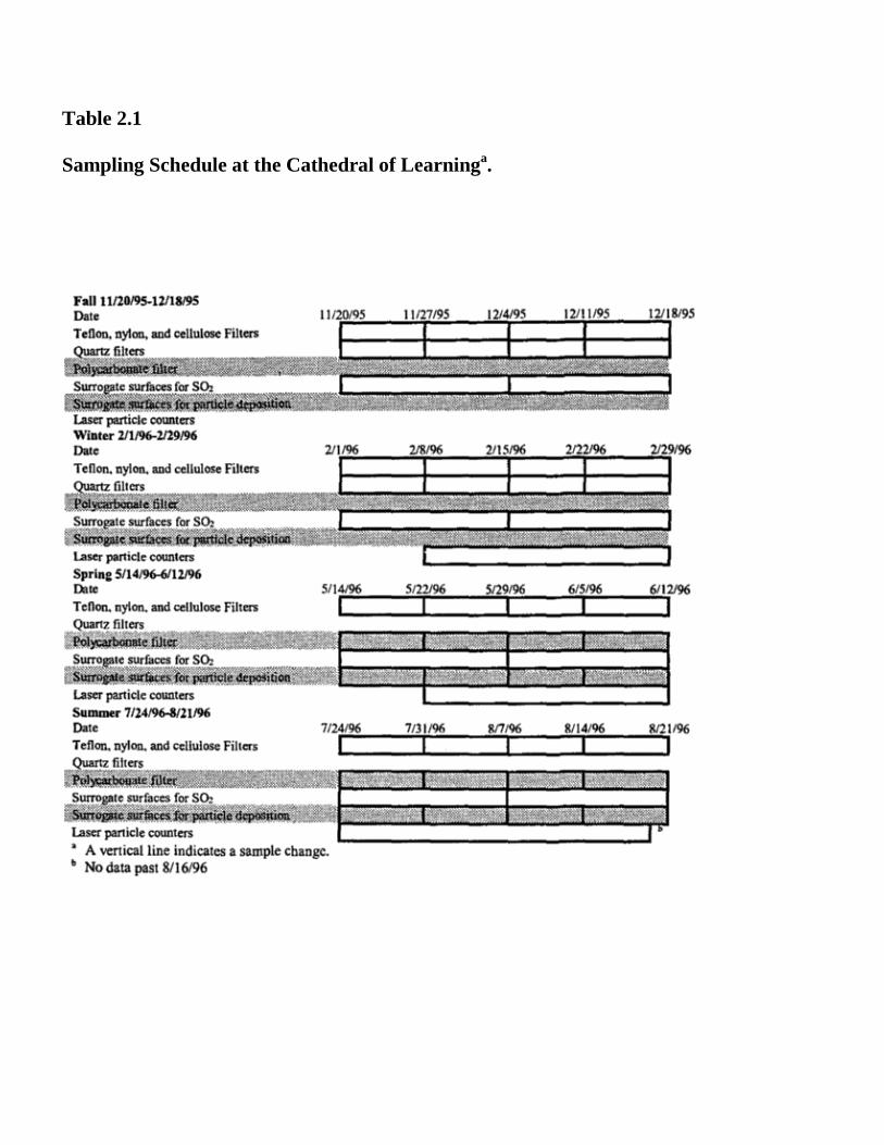
Table 2.1 Sampling Schedule at the Cathedral of Learninga.
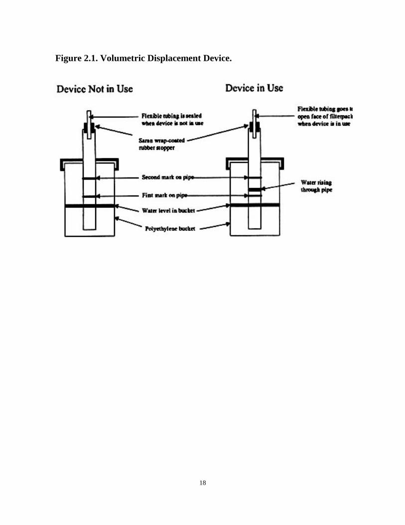
Figure 2.1. Volumetric Displacement Device.
18

Figure 2.2. Sampling Locations at the Cathedral of Learning. Locations 5-7 and 5-10 were not used
Figure 2.3. Surrogate Vertical Surfaces for Particle Deposition.
20

Figure 2.4. Schematic of Scanning Electron Microscope.
21

Figure 2.5. Scanning Electron Micrograph and Emission Spectrum for a Predominantly Aluminum Silicate Particle.
22

CHAPTER 3: AIRFLOW AND DELIVERY OF RAIN TO THE CATHEDRAL OF
LEARNING
3.1 INTRODUCTION
Estimating the extent to which surfaces, such as walls of a building, are exposed to rain is
essential for understanding the deterioration mechanisms for those surfaces. This is especiafly
true for historic calcareous stone structures since delivery of rain may have implications for the
rate of dissolution of calcite and gypsum (Mossotti and Eldeeb, 1994), productivity of harmful
microorganisms (Bock and Sand, 1993), and appearance of soiling patterns (Hamilton and
Mansfield, 1993). Experiments conducted at the Cathedral of Learning in 1995-1996 underscore
the importance of exposure of a limestone building to rain (Etyemezian et al., 1997, included in
Appendix A).
In general, the airflow near a solid obstacle such as a building has a profound impact on
the trajectory of an individual rain drop Wind approaching an obstacle such as a building must be
diverted, and this results in a change in the local wind velocities and causes a difference between
the velocity of a falling rain drop and the localized wind patterns. Because of friction and
aerodynamic pressure, the rain drop experiences a drag force. Qualitatively, the drag force
retards the motion of the drop towards the building Since most rain drops have diameters greater
than ~0.2 mm (Seinfeld, 1986), and therefore also have considerable inertia, the drag force may
not be sufficient to redirect the rain drop around the building. Consequently, some drops may
impinge on vertical surfaces such as walls.
This chapter is divided into three sections. First, we discuss the characteristics of airflow
around buildings in Section 3.2, with special focus on the distinctive features of the flow field Wind
tunnel studies have been a major source of information on this topic. Therefore, a brief discussion
on scaling parameters in wind tunnel experiments is also included. Second, we give an outline of
a computer model for rain delivery to a building (Section 3.3). The model is divided into two parts,
airflow simulation and rain drop trajectory calculation. Although this model is intended for use at
the Cathedral, the formulation 23

is not specific to any particular building Third, the contents of the chapter are summarized in
Section 3.4.
3.2 AIRFLOW AROUND A BUILDING
Airflow around buildings has received considerable attention in recent decades because
of the implications for the dispersion of pollutants emitted from nearby sources (e.g. Robins and
Castro, 1977a; Ogawa and Oikawa, 1983a; Snyder and Lawson, 1976). One of the primary
concerns is the entrainment of pollutants in the building wake cavity and the downwash of an
elevated plume as a result of the cavity. Consequently, much of the research has been geared
toward a better understanding of the flow separation that occurs at the leading edge as well as an
estimation of the size of the building wake cavity. Hosker (1984) has provided a comprehensive
review of studies conducted in this area of research through 1981.
The airflow over a bluff body, such as a building, is very complex. As a result, most
studies on such airflows have employed wind tunnel studies rather than field measurements.
Figure 3.1 illustrates some of the main features of the flow field. Typically, the flow of a fluid over a
bluff body at high Reynolds numbers can be divided into four regions: the windward faces, roof,
near wake, and far wake. The windward faces are expected to receive the most rain. Therefore,
flow patterns in this region are very important. Although we are not directly concerned with airflow
on the roof, the cavity formed in this area is closely linked with the flow over the windward face.
Likewise, flow patterns in the near wake of buildings are not directly pertinent to the impingement
of rain drops on windward faces. However, the cavity of the near wake is a major feature of flow in
the building envelope and therefore requires some attention. Characteristics of the far wake are not
discussed here. The discussion here focuses on incident flow normal to one side of the building,
although we briefly discuss the effect of incidence angle at the end of the section.
24

3.2.1 WIND TUNNEL MODELING
In order for wind tunnel data to be relevant to field conditions, certain characteristics of the
boundary layers in the atmosphere and the wind tunnel should be similar For example, we can assume
that the velocity profile in the region of the boundary layer to be modeled can be expressed as:
(3.1)
where U is the velocity at height z, and Ur and Zr are the reference velocity and reference height,
respectively. The boundary layers in the atmosphere and wind tunnel are considered similar if the
exponent n in Equation 3.1 is nearly the same for both situations (Plate, 1982). If the building height h is
larger than the atmospheric boundary layer height δ or if the influence of the airflow around the building is
not contained within the boundary layer, then there is an additional criterion that h/δ for the building and
for the model of the building in the wind tunnel should be similar. Boundary layer similarity is usually
achieved in the wind tunnel by placing appropriate roughness elements upstream of the model building.
Exact dynamic similarity can only be realized when the relevant dimensionless groups are
matched identically in the atmospheric and simulated flow. Some of these groups include the Rossby
number, Reynolds number, Richardson number, Prandtl number, and Eckert number. Of all these
parameters, only the Reynolds number Re has a significant effect in neutrally stratified boundary layer
flow. Here Re= Ur•Lr/ v, where Ur and Lr are respectively, the reference velocity and length scale, usually
taken as the building height, and v is the kinematic viscosity of air. Building models used in wind tunnels
are often at a scale of 1:1000. If exact Reynolds number similitude is to be achieved, freestream velocities
in wind tunnels would have to be about 1000 times the freestream velocities in the atmosphere.
Fortunately, for a boundary layer flow, the flow field becomes independent of Reynolds number (Re)
above a critical value and the major features of the flow can be captured in a wind tunnel. The critical
value needed to achieve Reynolds number independence ~10,000. Several authors discuss dynamic
similarity considerations for wind tunnel-simulated flow around buildings (Neff and Meroney 1996; Plate
1982; Snyder and Lawson 1976; Cermak 1976; Castro and Robins 1977; Saathoff et al (1995).
25
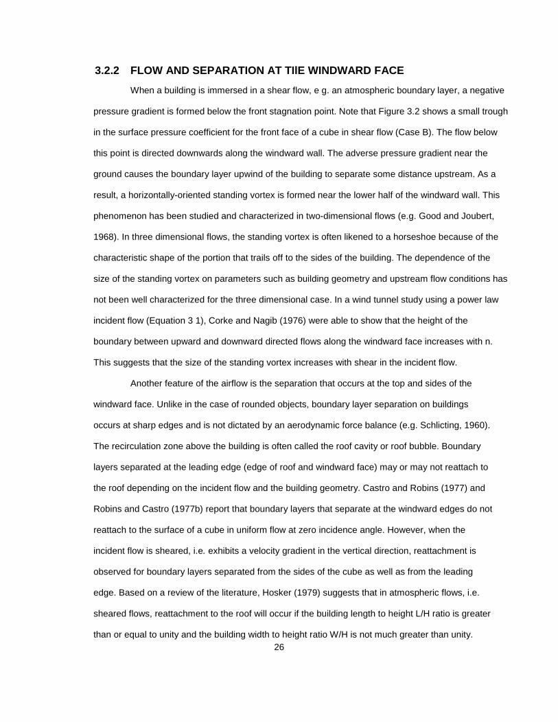
3.2.2 FLOW AND SEPARATION AT TIlE WINDWARD FACE When a building is immersed in a shear flow, e g. an atmospheric boundary layer, a negative
pressure gradient is formed below the front stagnation point. Note that Figure 3.2 shows a small trough
in the surface pressure coefficient for the front face of a cube in shear flow (Case B). The flow below
this point is directed downwards along the windward wall. The adverse pressure gradient near the
ground causes the boundary layer upwind of the building to separate some distance upstream. As a
result, a horizontally-oriented standing vortex is formed near the lower half of the windward wall. This
phenomenon has been studied and characterized in two-dimensional flows (e.g. Good and Joubert,
1968). In three dimensional flows, the standing vortex is often likened to a horseshoe because of the
characteristic shape of the portion that trails off to the sides of the building. The dependence of the
size of the standing vortex on parameters such as building geometry and upstream flow conditions has
not been well characterized for the three dimensional case. In a wind tunnel study using a power law
incident flow (Equation 3 1), Corke and Nagib (1976) were able to show that the height of the
boundary between upward and downward directed flows along the windward face increases with n.
This suggests that the size of the standing vortex increases with shear in the incident flow.
Another feature of the airflow is the separation that occurs at the top and sides of the
windward face. Unlike in the case of rounded objects, boundary layer separation on buildings
occurs at sharp edges and is not dictated by an aerodynamic force balance (e.g. Schlicting, 1960).
The recirculation zone above the building is often called the roof cavity or roof bubble. Boundary
layers separated at the leading edge (edge of roof and windward face) may or may not reattach to
the roof depending on the incident flow and the building geometry. Castro and Robins (1977) and
Robins and Castro (1977b) report that boundary layers that separate at the windward edges do not
reattach to the surface of a cube in uniform flow at zero incidence angle. However, when the
incident flow is sheared, i.e. exhibits a velocity gradient in the vertical direction, reattachment is
observed for boundary layers separated from the sides of the cube as well as from the leading
edge. Based on a review of the literature, Hosker (1979) suggests that in atmospheric flows, i.e.
sheared flows, reattachment to the roof will occur if the building length to height L/H ratio is greater
than or equal to unity and the building width to height ratio W/H is not much greater than unity. 26

3.2.3 THE NEAR WAKE REGION
After the flow separates from the windward edges of the building, it may either reattach to
the roof or sides, or to the ground at some distance downstream of the building. Reattachment on
the roof results in separation from the trailing edge on the leeward side of the building.
Consequently, the flow along the leeward face is directed upwards. Near the leeward face, the flow
along the ground is directed toward the building. If the boundary layer does reattach to the sides of
the building, two vertically oriented counter-rotating vortices are formed at the trailing edges where
the flow separates from the sides of the building once again (e.g. Ogawa et al., 1983b). This
phenomenon can be seen schematically in Figure 3. 1.
3.2.4 EFFECT OF WIND INCIDENCE ANGLE
Up to this point, the discussion has focused on incident wind normal to a side of the
building. Changing the incident wind angle has several repercussions. The majority of information
available is for incidence angles of 0° and 45°. It is instructive to highlight some of the major
differences in flow patterns between these two cases. Because of the wedge profile of the building
in the 45° case, a smaller fraction of the incident flow is diverted over the top of the building as
compared with the 0° case. Nevertheless, boundary layer separation does occur at the roof leading
edges (Castro and Robins, 1977). Unlike the case of 0° incidence, a separation bubble does not
appear on the roof Instead, a pair of counter-rotating vortices are created at the point where the two
leading edges meet In this geometry, the separated boundary layer does not reattach to the roof
(Hosker, 1984). Reattachment of the boundary layers separated from the roof and side edges does
occur on the ground further downstream of the building. However, the pattern of reattachment is
quite complex and heavily dependent on the incident wind profile (Ogawa et al, 1983b).
Similar to the case of 0° incidence, 45° incidence results in a pair of vertically oriented
counter-rotating vortices at the trailing edges. However, these vortices are much more pronounced
in the 45°
27

case (Ogawa et al., 1983b; Ogawa and Oikawa, 1982). In addition, the vortices, and indeed the entire flow
field, are more intermittent, even in the steady flow of a wind tunnel. This intermittence is due to the fact
that at 45° incidence, the stagnation point on the windward side is inherently unstable (Castro and Robins,
1977) and has a tendency to fluctuate across the plane of symmetry.
3.3 MODELING APPROACH
The calculation of rain drop trajectories around a building is a two-part process. First, the airflow
around the building must be determined. Second, the trajectory of rain subjected to the airflow must be
calculated. Other authors have investigated this two part process for various applications. Twohy and
Rogers (1993) calculate the delivery of rain drops to sampling instruments on aircraft In a similar study,
King and Dujmovic (1987) evaluate the impingement of snow on automobile windshields. However, in
both of these studies, the authors use potential flow theory to calculate the flow field, an approach that is
not applicable to inherently sheared flows such as in a boundary layer. Lakehal et al (1995) use the k-ε
model of turbulence to calculate the mean flow in a two dimensional street canyon and a Lagrangian
model to simulate rain drop trajectories. They also incorporate the effect of turbulence using a stochastic
method Finally, Choi (1993) uses a similar approach to simulate the trajectories of rain drops around a
building. However, he only considers normally incident flow using a generic shape for a building model.
3.3.1 AIRFLOW MODELING
Computational Fluid Dynamics (CFD) has become an increasingly popular method of studying
airfiows around and inside building environments (Scholes and Johnson, 1995). Advancements in
computing and in numerical techniques have rendered CFD a viable alternative to time-consuming wind
tunnel experiments and virtually unaffordable field experiments. In this project, the modeling of airflow
around the Cathedral of Learning will be accomplished numerically using the k- ε turbulence model.
Initially, the computer model will be run with a basic building shape such as a cube or rectangle. Results
from these model runs will be compared with field and wind tunnel data from the literature. Next, the
28

geometry of the building to be modeled wilt be altered to approach the geometry of the Cathedral of
Learning by the addition of smaller cubes and rectangles to the basic building shape.
There are several methods available for modeling turbulent flows numerically. They include
direct numerical simulation, one and two equation models of turbulence (Launder and Spalding, 1972),
and large eddy simulation (Deardorff, 1970), a combination of the former two In recent decades, a two
equation model, k-ε, has emerged as a popular technique for flow simulation. In this model, transport
equations for the turbulent kinetic energy (k) and the rate of energy dissipation (ε) are solved in
conjunction with the continuity and the Reynolds-averaged steady Navier-Stokes equations. The
formulation given by Launder and Spalding (1974) as it appears in Zhou and Stathopoulos (1996) is given
below:
29
(3.2)(continuity eqn). (3.3)(momentum eqn). (3.4)(k transport eqn). (3.5)(∉ transport eqn). (3.6) (3.7) (3.8) (3.9)

Ui ≡ mean velocity in x, direction ui ≡ fluctuating velocity in x, direction P ≡ augmented pressure Þ ≡ mean pressure ρ ≡ density of air k ≡ turbulent kinetic energy ∈ ≡ rate of energy dissipation νt ≡ eddy viscosity ν ≡ viscosity of air σ = l.0, σ2 =1.3,Cµ =0.09,C1 = 1.44, and C2 =1.92.
Equations 3 2-5 comprise a system of six equations and six unknowns (Equation 3.3 is actually
three equations, one for each of the Cartesian directions). They are solved numerically with the aid of a
finite element grid system and a set of boundary conditions. For this project, these equations will be
solved with the aid of commercially available software. Two software packages will be evaluated for
robustness, ease of use, and post-processing capabilities. These are ANSYS and FLUENT. The better
package, overall, will be used.
The computational domain for the flow around buildings (Figure 3 3) requires several different
types of boundary conditions. There are those at the inflow, the upper and side boundaries, and the solid
boundaries. There is some flexibility in choosing boundary conditions depending on the size of the
domain and the characteristics of the flow. At the inflow and upstream boundaries, the conditions for the
velocity components, k, and ε (Figure 3.4) are given by an assumed boundary layer profile (Zhou and
Stathopoulos, 1996). At the upper and side boundaries, tangential components of velocity, k, and ε are
Set to zero (Murakami and Mochida, 1989). On solid boundaries a form of the law of the wall is used
(Launder and Spalding, 1974; Patterson and Appelt, 1989; Murakami et al., 1996; Selvam, 1996;
Mikkelsen and Livesy, 1995). This boundary condition is based on the assumption that the velocity in the
boundary layer formed on a solid wall follows a logarithmic profile. Other researchers (e.g. Lam and
Bremhorst, 1979) have attempted to modify equations 3.2, 3.3, and 3.5 so that they apply from the fully
turbulent core through the viscous sublayer, thereby eliminating the need to assume a logarithmic profile
near the wall.
30

In its most simplified form, the Cathedral of Learning is a single rectangular structure. Detail
can be added to this basic form by appending additional cubic and rectangular pieces. Therefore, the
first step is to implement the k-ε airflow model for two basic building shapes, a rectangle and a cube.
Mode results for these shapes can then be compared with field and wind tunnel data from the literature.
Minson et al, (1995) have provided tabulated velocity information for a cube in a well characterized wind
tunnel low. These data are expressly intended for model testing by researchers in computational fluid
mechanics. However, airflow modeling results may also be compared with measurements by some of
the authors cited above (e.g. Castro and Robins, 1977, Ogawa et al., 1983b; Ogawa and Oikawa,
1982). Once the agreement between the computational model and literature data- for both 0° and 45°
incident flows- is acceptable, the geometry of the basic building model can be altered by the gradual
addition of detail. At some point, further detail ceases to improve the quality of the results and requires
higher computational effort. Thus, the degree of complexity of the model building is not without bounds.
3.3.2 RAIN DROP SIZE DISTRIBUTIONS AND TRAJECTORIES
The equations of motion for a single rain drop can be written as:
(3.10) M ≡ particle mass Up
i ≡ if particle velocity in xi direction FDi ≡ drag force in xi direction G ≡ gravitaional constant δif ≡ delta function; δif , =1 if I = j, δif = 0 if i≠ j.
The form of FD depends on the relative velocity of the drop in the flow field and the drag
coefficient, which is based on the assumed shape of the drop. Note that a rain drop moving through the
air experiences aerodynamic pressure forces that can alter its shape. Qualitatively, drops with diameter
greater than -200 µm are too large to retain a spherical shape at their terminal velocities. At these large
sizes, drops form, on average, a spherical obloid shape as shown in Figure 3.5 (Beard and Chuang, 31

1987; Ramaswamy, 1979; Reizebos and Epema, 1985). Furthermore, because of perturbations in the airflow at
the drop surface, the instantaneous shape may be quite variable (Beard and Chuang, 1987). These complexities
coupled with an absence of data on drop shapes at relative velocities different from the terminal velocity require
that a simplifying assumption be made. Other investigators have assumed that the drag coefficient for a rain drop
is identical to that of a sphere (Lakehal et al., 1995; Twohy and Rogers, 1992) and this assumption Will be
adopted for the present model. The resulting equation for FD becomes:
(3.11)
CD ≡ coefficient of drag f(Re)
Re sphere Reynolds number =
r ≡ raindrop diameter
ρ ≡ density of air
υ ≡ kinematic viscosity of air.
The size distribution of rain drops in free fall is determined by the competing processes of drop breakup
and coalescence (Brown and Whittlesey, 1992). Larger rain drops have higher terminal velocities than smaller
ones. Consequently, collisions between rain drops occur somewhat frequently. On the other hand, large drops
are unstable and tend to break up into smaller drops (Alusa, 1975). The result is an equilibrium size
distribution similar to the one shown in Figure 3.6. The theoretical model for this size distribution has the
attractive property that its shape does not vary with rainfall intensity (Gillespie and List, 1978/1979). However,
caution must be exercised before this model is used and a comparison with measured field data is necessary.
These data may be obtained either from the literature or from measurements at the Cathedral of Learning.
The possibility of using a disdrometer to sample rain drop sizes is being investigated. A disdrometer is a
simple instrument fashioned after a sensitive scale (Loffler-Mang et al., 1996). Individual rain drops impinging
on a horizontal plate cause the plate to move slightly (Figure 3.7). A series of springs and inductor coils
generate an electrical signal each time the horizontal plate is moved.
32

The sizes of the impinging rain drops are then deduced based on this signal. At this time, it is unclear if
the use of a disdrometer at the Cathedral of Learning is feasible.
3.3.3 RAIN IMPINGEMENT: FIELD DATA
The rain trajectory model is expected to generate three output parameters: the flux of rain to the
building surface (measured in units of mass per unit time per unit building surface area) and the normal
and tangential impingement velocities for rain drops of different sizes. Development of a device to
measure rain flux to the walls of the Cathedral of Learning is currently underway. Sheets of thin PVC at
being used as vertical rain collection surfaces on the roof of Porter Hall on the Carnegie Mellon
University campus. If these preliminary experiments are successful, then similar devices can be used a
surrogate surfaces for incident rain collection at the Cathedral of Learning. Data gathered from these
devices can be compared with model predictions.
Rain impingement modeling results can also be compared with soiling patterns directly. For
example, the spatial distributions of impingement velocities for individual rain drops can be transformed
into distributions of momentum flux to the walls. These can then be compared with observed soiling
patterns at the Cathedral of Learning, assuming that regions of high impingement velocities will have
greater erosion of surface material and therefore less visible blackness.
3.4 SUMMARY
Results from experiments conducted in 1995-1996 (Appendix A) suggested that the delivery of
rain to the Cathedral walls is an important process. Based on these findings, a modeling effort geared
toward a better understanding of rain trajectories around buildings, and the Cathedral in particular, has
been proposed. The simulation of airflow around a building will be accomplished numerically with the k-ε
model for turbulence Initial results, based on simple building geometries, will bi compared with data
available from the literature. Degrees of complexity will be added to the geometry subsequently until an
optimum level of detail is achieved. Rain trajectories near and around the building model will be
calculated based on simple equations of motion and the assumption that drag coefficients 33

for rain drops are similar to those for a sphere. Rain drop size distributions will be obtained from the
literature and, if possible, measured at a location near the Cathedral of Learning. It initial tests are
successful, rain fluxes to the Cathedral walls will be measured with PVC surrogate surfaces for rain
collection and compared to those from modeling results. Finally, soiling patterns at the Cathedral will be
compared with output parameters from the rain trajectory model.
34

Figure 3.1. Model of Flow Near a Sharp-Edged Three-Dimensional Building in a Deep Boundary Layer. Hosker (1984).
35

Figure 3.2. Surface Pressure Coefficient on a Cube in a Wind Tunnel. Castro and Robins (1977).
The incident flow is uniform in case A and in case B the boundary layer depth is 10 times the cube height. cpm(ps – pr)/1/2ρU2
r where ps , pr , and Ur are the static surface pressure and the reference pressure and velocity, taken at the wind tunnel exit.
36

Figure 3.3. Example of Computational Grid System for a Cube in a Boundary Layer. Zhou and Stathopoulos (1996).
x, y, and z are the streamwise, transverse, and vertical directions
37

Figure 3.4. Example Profiles of Incident Flow Boundary Conditions. Zhou and Stathopoulos (1996).
Computational domain extends to z 70 cm. Here, U is the velocity at height z, Ug is the velocity in the freestream, Ub is the velocity at the building height H, k and e (ε) are the kinetic energy and energy dissipation rate.
38

Figure 3.5. Computed Shapes of Rain drops of Various Equivalent Diameters.
Beard and Chuang (1987).
Computation based on a balance between hydrostatic pressure, aerodynamic pressure, and surface tension forces.
39
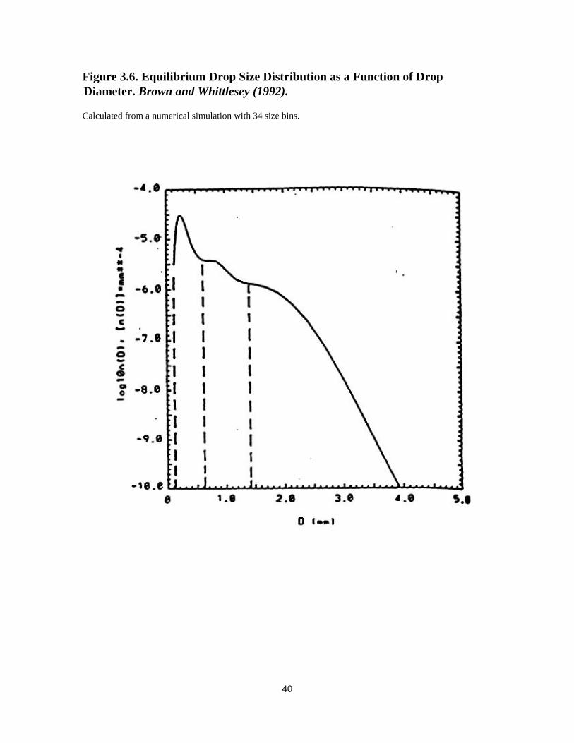
Figure 3.6. Equilibrium Drop Size Distribution as a Function of Drop Diameter. Brown and Whittlesey (1992).
Calculated from a numerical simulation with 34 size bins.
40
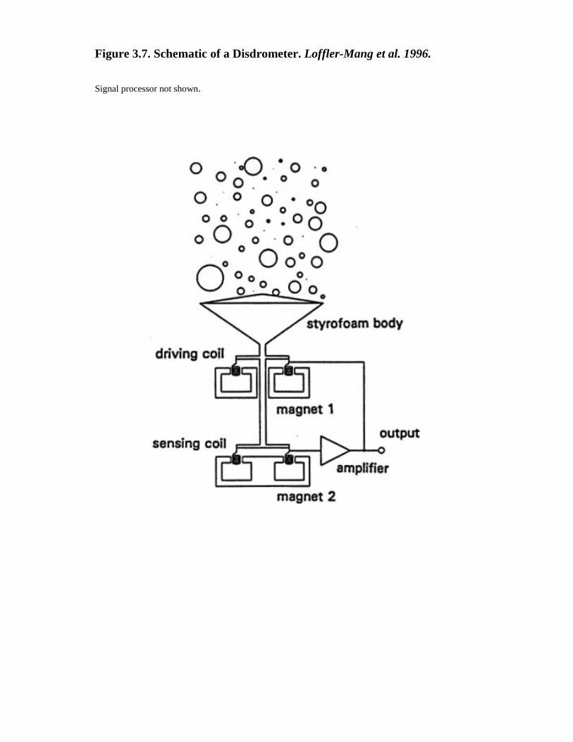
Figure 3.7. Schematic of a Disdrometer. Loffler-Mang et al. 1996.
Signal processor not shown.
4
1

CHAPTER 4: REPORT SUMMARY This project has focused on obtaining a better understanding of chemical and physical processes that further the
deterioration of calcareous stone buildings. Investigation of such processes has occurred primarily at the 42-story
Cathedral of Learning. However, some of the results obtained at the Cathedral can be extended to other limestone
buildings in similar environments. Such information can aid conservators in assessing mechanisms of damage or in
deciding on appropriate treatments for deteriorating buildings.
This report summarizes work conducted on the Cathedral of Learning project during November 15, 1996 and
November 15. 1997. Specifically, we have reported on the status of two on-going research efforts. First, we described
experiments at the Cathedral where particles were collected on air sampling filters as well as surrogate surfaces for
vertical deposition. These samples were obtained during spring and summer 1996 as part of a larger study in which
vertical gradients of pollutant concentrations and deposition fluxes were measured (Etyemezian et al., 1997;
Appendix A). Scanning electron microscopy analysis on a limited number of samples suggests the presence of at
least three types of particles, 1) calcium, sulfur, and silicon rich (Ca-S-Si), 2), aluminum, silicon, and iron rich (Al-
Si-Fe), and 3) calcium and magnesium rich (Ca-Mg). Preliminary results also indicate that size distributions of
particles found on air filters are different from those found on surrogate surfaces.
Second, we have described the development of two models: A computer model for describing airflow around the
Cathedral, and a simple mathematical model for calculating trajectories of individual raindrops. The airflow model
will utilize commercially available computational fluid dynamics software. Initially, the model will be used with
basic building shapes such as cubes and rectangles. Results with these shapes will be compared with field and wind
tunnel data from the literature. In later studies, we will use building shapes that better represent the geometry of the
Cathedral. The airflow model will provide input parameters for other modeling efforts including the calculation of
raindrop trajectories near the Cathedral..
42

REFERENCES Alusa, AL. . 1975. The Role of Drop Breakup in the Development of Rain drop Size Distributions. Journal de Recherches Atmosphericues 9 (1):1-10. Amoroso, G.G., and V. Fassina 1983. Stone Decay and Conservation: Atmospheric Pollution, Cleaning, Consolidation and Protection, Materials Science Monographs 11, Elsevier, 1983. Beard, K.V., and C. Chuang. 1987. A New Model for the Equilibrium Shape of Rain drops. Journal of the Atmospheric Sciences 44 (11): 1509-1524. Bock, E., and W. Sand. 1993. The Microbiology of Masonry Biodeterioration Journal of Applied Bacteriology 74: 503-514. Brown, P.S. Jr., and S.N. Whittlesey. 1992. Multiple Equilibrium Solutions in Bleck-Type Models of Drop Coalescence and Breakup. Journal of Atmospheric Sciences 49 (23): 2319-2324. Camuffo, D., M. Del Monte, C. Sabbioni, and O. Vittori. 1982. Wetting, Deterioration and Visual Features of Stone Surfaces in an Urban Area. Atmospheric Environment 16(9): 2253-2259. Castro, I.P., and A.G. Robins. 1977. The Flow around a Surface-Mounted Cube in Uniform and Turbulent Streams. Journal of Fluid Mechanics 79 (2): 307-335. Cermak, J.E., 1976. Aerodynamics of Buildings. In Annual Review of Fluid Mechanics 8: 75-106. Annual Reviews, Inc. Palo Alto, CA. 1976. Choi, E.C.C.1993. Simulation of Wind-Driven Rain around a Building. Journal of Wind Engineering and Industrial Aerodynamics 46: 721-729. Corke, T.C., and H.M. Nagib. 1976. As Cited in Hosker (1984). Sensitivity of Flow around and Pressures on a Building Model to Changes in Simulated Atmospheric Surface Layer Characteristics. lIT Fluids and Heat Transfer Report R76-1, May, Illinois Institute of Technology, Mechanics and Mechanical and Aerospace Engineering Deaprtment, Chicago, Illinois. Davidson, C.I., and V.L. Wu. 1990. Dry Deposition of Particles and Vapors. Chapter 3 in Acid Precipitation, Volume 2. Sources, Emissions, and Modeling, D.C. Adriano ed., Advances in Environmental Sciences Series, Springer-Verlag, New York. Deardorff, J.W.. 1969. A Numerical Study of Three-Dimensional Turbulent Flow at Large Reynolds Numbers Journal of Fluid Mechanics 41 (2): 453-480. Del Monte, M., C. Sabbioni, and O. Vittori. 1981, Airborne Carbon Particles and Marble Deterioration, Atmospheric Environmentl5: 645-652. Etyemezian, V., C.I. Davidson, S. Finger et al. 1995. Influence of Atmospheric Pollutants on Soiling of a Limestone Building Surface Progress Report for the NatiOnal Park Service. September, 1995. Etyemezian, V., C.I. Davidson, S. Finger et al. 1996. Vertical Gradients of Pollutant Concentrations and Deposition Fluxes at the Cathedral of Learning. Progress Report for the National Park Service. November, 1996.
43

Etyemezian, V E., C.I. Davidson, S. Finger, M. Striegel, N. Barabas, and J. Chow 1997. Vertical Gradients of Pollutant Concentrations and Deposition Fluxes on a Tall Limestone Building. Submitted to the Journal of the American Institute for Conservation, November 1997. Flagan, R.C., and J. H. Seinfeld. 1988. Fundamentals of Air Pollution Engineering. Prentice-Hall, New Jersey. Freemantle, M. 1996. Historic Monuments Pose Challenge to Conservation Scientists Chemical and Engineering News 74: 20-23. Friedlander, S.K. 1977. Smoke, Dust, and Haze- Fundamentals of Aerosol Behavior, Wiley, New York.
Gillespie. J.R., and R. List. 1978/1979. As cited in Brown and Whittlesey (1992). Effects of Collision-Induced Breakup on Dropsize Distributions in Steady-State Rain-Shafts. Pure Applied Geophysics 117: 599 –626. Good, M.C., and P.N. Joubert. 1968. The Form Drag of Two-Dimensional Bluff-Plates Immersed in Turbulent Boundary Layers. Journal of Fluid Mechanics 31 (3): 547-582. Hamilton, R.J., and T.A. Mansfield. 1993. The Soiling of Materials in the Ambient Atmosphere. Atmospheric Environment 27a (8): 1369-1374. Hosker, R.P.Jr., 1979. As cited in Hosker (1984). Empirical Estimation of Wake Cavity Size Behind Block-Type Structures. In Preprints of Fourth Symposium or Turbulence, Diffusion, and Air Pollution, Rena, Nevada. January, pp 603-609, American Meteorological Society, Boston, MA, 1979. Hosker, R.P.Jr., 1984. Flow and Diffusion near Obstacles In: Atmospheric Science and Power Production Report for United States Department of Energy. Darryl Randerson, editor. Hutchinson, A.J., J.B.Johnson, G.E.Thompson, G.C. Wood, P.W. Sage, and M.J. Cooke. 1992. The Role of Fly-ash Particulate Material and Oxide Catalysts in Stone Degradation. Atmospheric Environment 26a: 2795-2803. King, W.D., and S.Dujmovic. 1987. Fluid Flow and Particle Trajectories around Simple Bodies: Impaction of Snowflakes on Car Windshields. American Journal of Physics 55(2): 149-154. Lakehal, D., P.G. Mestayer, J.B. Edson, S. Anquetin and J.F. Sini. 1995. Eulero-Lagrangian Simulation of Rain drop Trajectories and Impacts within the Urban Canopy Atmospheric Environment 29: 3501-3517. Lam, C.K.G., and K. Bremhorst. 1981. A Modified Form of the K-ε Model for Predicting Wall Turbulence. Journal of Fluids Engineering 103: 456-460. Launder, B.E., and D.B. Spalding. 1972. Lectures in Mathematical Models of Turbulence. Academic Press London, England. Launder, B.E., and D.B. Spalding. 1974. The Numerical Calculation of Turbulent Flows. Computer Methods in Applied Mechanics and Engineering 3: 269-289. Loffler-Mang, M., K.D. Beheng,, and H.G. Karlruhe. 1996. Drop Size Distribution Measurements in Rain-a Comparison of Two Sizing Methods. Meteorol. Zeitschrift 5: 139-144. McGee, E.S. 1997. Surficial Alteration at the Cathedral of Learning in Pittsburgh, Pennsylvania. USGS Open-File Report 97-275.
44

Mikkelsen, A.C., and F.M. Livesey. 1995. Evaluation of the Use of the Numerical K-ε Model Kameleon II, for Predicting Wind Pressures an Building Surfaces. Journal of Wind Engineering and Industrial Aerodynamics 57: 375-389. Minson A.J., C.J. Wood, and R.E. Belcher. 1995. Experimental Velocity Measurements for CFD Validation. Journal of Wind Engineering and Industrial Aerodynamics 58: 205-215. Mossotti, V.G., and A.R. Eldeeb. 1994. Calcareous Stone Dissolution by Acid Rain. Manuscript in progress. Version-0 7, Dec. 12, 1994. Murakami, S., and A. Mochida. 1989. Three-Dimensional Numerical Simulation of Turbulent Flow around Buildings Using the k- ε Model. Building and Environment 24(1): 51-64. Murakami, S., A. Mochida, R. Ooka. S. Kato, and S. lizuka. 1996. Numerical Prediction of Flow around a Building with Various Turbulence Models Caomparison of k- ε EVM, ASM, DSM, and LES with Wind Tunnel Tests. ASHRAE Transactions 102(1): 741-753. Neff, D.E., and R.N. Meroney. 1996. Reynolds Number Independence of the Wind Tunnel Simulation of Transport and Dispersion about Buildings. Unpublished Report 23 pages. 15 references. Nord, A.G., A. Svardh, and K. Tronner. 1994. Air Pollution Levels Reflected in Deposits on Building Stone. Atmospheric Environment 28(16): 2615-2622. Ogawa, Y. and S. Oikawa. 1982. A Field Investigation of the Flow and Diffusion around a Model Cube. Atmospheric Environment 16: 207-222. Ogawa, Y. S. Oikawa, and K. Uehara. 1983a. Field and Wind Tunnel Study of the Flow and Diffusion around a Model Cube-Il. Nearfield and Cube Surface Flow and Concentration Patterns. Atmospheric Environment 17: 1161-1171. Ogawa, V., S. Oikawa, and K. Uehara. 1983b. Field and Wind Tunnel Study of the Flow and Diffusion around a Model Cube-I. Flow Measurements. Atmospheric Environment 17: 1145-1159. Paterson, D.A., and C.J. Apelt. 1989. Simulation of Wind Flow around Three-Dimensional Buildings. Building and Environment 24(1): 39-50. Plate, E., 1982. Wind Tunnel Modelling of Wind Effects in Engineering. In: Engineering Meteorology vol I. E.Plate, editor, Elsevier, Amsterdam, Oxford, and New York. 573-640. Ramaswamy, V., and P. Chylek. 1979. Shape of Rain drops. In Proceedings of the International Workshop on Light Scattering by Irregularly Shaped Particles. June, 1979. 334 pages. pp 55-61. Plenum, Albany, New York. 1979. Riezebos, H.T., and G.F. Epema. 1985. Drop Shape and Erosivity Part II: Splash Detachment, Transport, and Erosivity Indices. Earth Surface Processes and Landforms 10: 69-74. Robins. A.G., and I.P. Castro. 1977a. A Wind Tunnel Investigation of Plume Dispersion in the Vicinity of a Surface Mounted Cube-Il. The Concentration Field. Atmospheric Environment 11: 299-311. Robins, A.G., and I.P. Castro. 1977b. A Wind Tunnel Investigation of Plume Dispersion in the Vicinity of a Surface Mounted Cube-I. The Flow Field. Atmospheric Environment 11: 291-297. Saathoff, P.J., T. Stathopoulos, and M. Dobrescu. 1995. Effects of Model Scale in Estimating Pollutant Dispersion near Buildings. Journal of Wind Engineering and Industrial Aerodynamics 54: 549-559.
45

Sabbioni, C. 1994. Effects of Air Pollution on Historic Buildings and Monuments Scientific Basis for Conservation Physical, Chemical, and Biological Weathering. European Cultural Heritage Newsletter on Research 8 (1): 2-6. Schlichting, H., 1960. Boundary Layer Theory, 4th ed., McGraw Hill, New York, London, and Paris. Scholes, A.J., and I.H.Johnson. 1995. Impact of CFD Techniques on Environmental Engineering Environmental Engineering 8 (2): 12-17. Schwoeble, A.J., H.P.Lentz, W.J. Mershon, and G.S. Casuccio. 1990. Microimagining and Off-line Microscopy of Fine Particles and Inclusions. Materials Science and Engineering a124: 49-54. Seinfeld, J.H. 1986. Atmospheric Chemistry and Physics of Air Pollution John Wiley and Sons, New York.
Selvam, R.P. 1996. Numerical Simulation of Flow and Pressure around a Building ASHRAE Transactions 102(1): 765-772. Snyder, W.H., and R.E. Lawson Jr. 1976. Determination of a Necessary Stack Height for a Stack Close to a Building. A Wind Tunnel Study. Atmospheric Environment 10: 683-691. Twohy, C.H., and D. Rogers. 1993. Airflow and Water-Drop Trajectories at Instrument Sampling Points around the Beechcraft King Air and Lockheed Electra. Journal of AtmosDheric and Oceanic Technology 10: 566-578. Wilmzig, M., and E. Bock 1995. Endangerment of Mortars by Nitrifiers, Heterotrophic Bacteria and Fungi. In Biodeterioration and Biodegradation 9 eds. A Bousher et al., Institution of Chemical Engineers, Rugby, UK, 195-197. Young, P. 1996b. Mouldering Monuments. New Scientist 152: 37-38. Zhou, Y., and T. Stathopoulos. 1996. Application of Two-Layer Methods for the Evaluation of Wind Effects on a Cubic Building. ASHRAE Transactions 102(1): 754-764.
46

APPENDIX A: VERTICAL GRADIENTS OF POLLUTANT CONCENTRATIONS AND DEPOSITION
FLUXES TO A TALL LIMESTONE BUILDING. MANUSCRIPT SUBMITTED TO JAIC ON NOVEMBER
11, 1997.
47

Etyemezian et al. p.1
Vertical Gradients of Pollutant Concentrations and Deposition Fluxes on a Tall Limestone Building
V. Etyemezian1*, C.I. Davidson1 , S. Finger1, M. Striegel2, N. Barabas3, and J. Chow4
*Corresponding Author
1Deptartment of Civil and Environmental Engineering
Carnegie Mellon University Pittsburgh, PA 15213
2NationaI Center for Preservation Technology and Training
NSU Box 5682 Natchitoches, LA 71497
3Department of Civil and Environmental Engineering
University of Michigan 116 EWRE Building 1351 Beat Avenue
Ann Arbor. MI 48109
4Desert Research Institute 5625 Fox Avenue P.O. Box 60220 Reno, NV 89506
Submitted to the Journal of the American Institute for Conservation
Manuscript: DO NOT CITE OR CIRCULATE
11/10/97
Etyemezian et al. p.2
1. ABSTRACT
The role of air pollutants in the soiling of a limestone building was investigated by measuring pollutant airborne
concentrations and deposition at different heights at the Cathedral of Learning in Pittsburgh, Pennsylvania.
Airborne concentrations of SO42- particles, carbon particles, SO2 gas, and total NO3 (particles + HNO3) were
measured simultaneously on the fifth floor, sixteenth floor, and roof (forty-second floor), while laser particle
counts of>0.5 µm and >5 µm particles were obtained on the fifth and sixteenth floors. SO2 deposition fluxes to
wall-mounted surrogate surfaces were measured at a total of nine locations on the fifth and sixteenth floors.
Measurements were conducted during four time periods over the course of one year, each time period lasting four
weeks. Results showed that airborne concentrations of the chemical species were invariant with height. Airborne
number concentrations of>0.5 µm particles corroborated this result. Although not reflected in the chemical data,
measured number concentrations of>5 µm particles on the sixteenth floor were on average 30% greater than those
on the fifth floor. The spatially averaged highest and lowest deposition velocities of SO2 (1.0 cm/s and 0.6 cm/s)
never differed by more than a factor of two for the different time periods. The relative differences in deposition
velocities from one location to another were consistent throughout all of the sampling experiments. Sixteenth
floor deposition velocities were greater than those on the fifth floor but this was due, at least in part, to the fact
that sampling locations on the sixteenth floor were more exposed to wind. The absence of gradients suggests that
soiling patterns on the Cathedral are determined by the competing processes of pollutant deposition and rain
washing. This hypothesis is supported by comparing soiling patterns on the Cathedral from the 1930’s with recent
patterns: Archival photographs show much greater amounts of soiling, consistent with the greater air pollution
levels that existed then. Results of this study can assist in designing cleaning and treatment protocols for other
buildings with similar geometry in similar environments.
2. INTRODUCTION
Several types of building stone deterioration have been well documented, including discoloration, erosion of
material, and changes in the physical and chemical characteristics of the surface. Developing strategies to prevent
this deterioration requires knowledge of the processes by which the damage occurs, for example

Elyemezian et al p3
by deposition of air pollutants or by biological growth on the stone surface. Furthermore, the choice of cleaning
and restoration techniques depends on the processes causing the damage.
Differentiation between pollutant deposition and biological growth is difficult and generally requires on-site
testing. Unfortunately, getting access to the building walls sometimes demands scaffolding, and due to expense
scaffolds are typically not erected until shortly before restoration work begins Thus, early identification of the
primary deteriorating or discoloring agents is oflen difficult and tentative.
In this study, field measurements of air pollutant concentrations and deposition are used in conjunction with
archival photographs to draw conclusions regarding the role of pollutants in the soiling of a tall building. The
structure of interest is the 42-story Cathedral of Learning, a National Historic Landmark on the University of
Pittsburgh campus (Figure 1). The building is made of Indiana limestone and was constructed between 1929 and
1937 Since the time of construction, there have been numerous air pollution sources within a few kilometers of the
building. These include steel manufacturing plants that employ coke ovens and blast furnaces, a coal-burning steam
plant, heavy motor vehicle traffic, coal-burning railroads and riverboats, and a large number of domestic coal
combustion sources such as home furnaces
At present, two sides of the Cathedral of Learning have extensive soiling, particularly on the lower two-
thirds of the building In a study on the alteration crust at the Cathedral, McGee (1995; 1997) reports that Fe-, Si-. and
Al- rich fly ash particles are found in samples of soiled surfaces and that such particles are much less prevalent in
samples of unsoiled surfaces. This result indicates that surface soiling at the Cathedral is primarily due to deposition
of anthropogenic particles to the building walls.
This research had three major objectives. First, we wanted to identify the extent to which airborne
concentrations of certain pollutants vary with height on the Cathedral. The pollutants of interest include SO42-
particles, carbon particles. SO2 gas, total NO3- (HNO3 gas and NO3
- particles), and total particle number. Such
information can provide insight on the relative importance of local and regional sources of pollutants as well as
pathways for delivery of pollutants to the building surface. Second, we wished to examine variations in dry
deposition of SO2 with height and location. This can provide information on whether the variability in pollutant
deposition is partly responsible for the observed soiling patterns. Third, we wished to consider long-term variations
in soiling patterns on the building in light of changes in pollution concentrations. This part of the project made use of
previously obtained historical pollutant data

Etycmezian et al. p.4
as well as archival photographs. Such information enabled us to investigate the roles of pollutant deposition and
subsequent washoff by rain in affecting the soiling. Although this study focused on only one building, the results
may also be applicable to geometrically similar buildings in similar environments.
3. BACKGROUND
Calcareous stones exposed to the atmosphere are vulnerable to attack by several processes which occur
naturally. These processes include microbial activity on the stone surface, dissolution by rain, and
physical stresses such as freeze-thaw cycles. Anthropogenic air pollutants are frequently responsible for
accelerated deterioration, both directly through physical and chemical attack, and indirectly by providing
substrates for microbial growth.
In recent years,considerable attention has been given to the role of biological agents in damage to
buildings (e.g. Young. 1996a: Freemantle, 1996. Wilmzig and Bock. 1995: Mitchell et al. 1996). In
general, species of fungi, algae, lichens, and bacteria have been found on surfaces of building stones
(Bock and Sand. 1993). These organisms can accelerate deterioration either by physical processes such as
alteration of the normal wetting-drying cycle (Young. l996b), or by chemical processes such as mineral
and organic acid production and secretion of metal-chelating agents (Palmer et al., 1991). It is difficult to
estimate the quantities and overall effects of biodeteriogens, in part because the fecundity and
productivity of these organisms is strongly dependent on microenvironmental factors. These include
insolation, stone type and porosity, surface and air temperatures, availability of a suitable substrate, and
availability of water from incident rain, stone pore capillarity, or condensation and evaporation cycles
(Bock and Sand. 1993). In addition to the expected temporal variability caused by changes in the weather
(Tayler and May, 1991), there can be considerable spatial variability over short distance scales
Understanding biodeterioration processes is further confounded by a possible correlation between air
pollution levels and biodeterioration rates (Young, 1996b). For example, Warscheid et al (1991) have
shown that some chemo-organotrophic bacteria isolated from sandstones of historic monuments are able
to utilize petroleum derivatives as sources of carbon as well as energy.

Etyemezian et al. p.5
Several categories of air pollutants can accelerate the natural deterioration of Stone through two
primary processes, wet and dry deposition (e.g. Sherwood et al., 1990, Anioroso and Fassina, 1933). The
former refers to the deposition of a pollutant by a precipitation process such as rain or snow; acid rain is an
example. Several authors have considered the effects of acid rain on calcareous stones (Winkler, 1996; Braun
and Wilson, 1970; Mossotti and Eldeeb, 1994; Livingston, 1992; Hutchinson et at., 1993). Dry deposition
includes those process by which pollutants are transported to the surface in the absence of precipitation and
become physically or chemically bound to the surface. Damage to calcareous building stone by dry
deposition has been attributed largely to sulfur dioxide gas (SO2). For example, Meierding (1993) found that
mean surface recession rates of century-old Vermont marble tombstones in the United States were well
correlated with SO2 concentrations. In addition, some authors point out that nitric acid gas (HNO3) may also
be sorbed onto a carbonate surface (Kirkitsos and Sikiotis, 1995; Fenter et al., 1995).
The removal of SO2 by certain stone twes is a well-documented phenomenon (Judeikis et al 1978).
Calcareous stones subjected to high relative humidity develop a moist surface layer where SO2 can readily
dissolve (Spiker et al., 1995; Spedding, 1969); in general, the rate of dissolution increases at higher relative
humidities and wind speeds (Spiker et al., 1995). Dissolved SO2 can then oxidize to form a sulfite (SO32-) or
sulfate (SO42-) species. The oxidation process results in the production of acid which can cause the calcium
carbonate (CaCO3) in the stone to dissolve. When calcium ions (Ca2+) combine with SO32- or SO4
2-, CO32- is
effectively displaced from the stone surface. This process, known as sulfation, may also involve gaseous and
particulate air pollutants other than sulfur species. Gases such as ozone (O3) (Haneefet al., 1992) and
nitrogen dioxide (NO2) (Johansson et al., 1988) have been shown to increase SO2 deposition to limestone.
Surface crust analyses of damaged stone have also shown a close relation between deposited anthropogenic
particles and the formation of gypsum crystals (Zappia, 1993; Sabbioni, 1994; Del Monte et al., 1981),
suggesting a relationship between sulfation and the presence of airborne particles. However. Hutchinson et
al. (1992) have reported that limestone seeded with coal fly ash or transition metal oxide catalysts is not
susceptible to elevated SO2 deposition. These authors suggest that seeding stone samples with oxidation
catalysts has a negligible effect because natural stones already contain high levels of impurities. In contrast,
seeding pure CaCO3 with metal oxide catalysts does increase the rate of sulfation.

Etyemezian et al. p.6
Urban air pollution studies have considered effects of buildings on dispersion of vehicle emissions
as well as dispersion of individual plumes from stationary sources. In general, dispersion of vehicle
emissions in street canyons is a function of the building height divided by the street width, known as the
aspect ratio (Lee and Park, 1994), as well as the geometric configurations of city blocks, the ambient wind
direction, and the movement of motor vehicles (DePaul and Sheih, 1985; Dabbert and Hoydysh, 1991;
Hoydysh and Dabbert, 1994). Qin and Chan (1993) and Qin and Kot (1993) have reported that significant
differences in carbon monoxide and nitrogen oxides (NOx) concentrations exist between the top and bottom
of buildings surrounding Street canyons in Guangzhou. China Qin and Kot (1990) have also shown that
vehicle traffic near a 31 Story (100 m) tower can result in elevated NOx concentrations near the downwind
building surface up to a height of 66 meters. The effect of a building on the dispersion of a stationary source
plume is, in general, dependent on the building geometry, source location, and prevailing wind conditions
(e.g. Lee Ct al., 1991; Huber et al., 1991; Thompson. 1993). In some eases, direct measurement of the spatial
variability of surface concentrations may be easier than application of theoretical considerations.
4. EXPERIMENTAL
Vertical gradients of pollutant concentrations and deposition fluxes were measured by sampling at varying
elevations on the Cathedral of Learning. Three locations were chosen for sampling: the fifth floor and
sixteenth floor patios on the southeastern façade and the patio on the roof (Figure 2). The southeastern façade
was chosen for two reasons. First, it was one of the two heavily soiled sides of the building (the northeastern
façade being the other). Second, the fifth floor and sixteenth floor patios on the southeastern façade were
frequently on the windward side of the Cathedral (Figure 3) where mixing is not affected by the wake cavity
of the building.
The vertical gradient experiments were conducted on four separate occasions from the period of
11/20/95 to 8/21/96. The experiments were scheduled so that representative sets of data were obtained during
the different seasons of the year (Table 1). Each set of experiments included four consecutive sampling
periods of one week each. Sampling was uninterrupted throughout this period except for

Etyemezian et al. p.7
approximately three hours each week for changing samples. Airborne concentrations of SO42- particles, SO2 gas,
and total NO3- species (NO3
- particles and HNO3 gas) were measured. Airborne concentrations of elemental and
organic carbon particles were measured during the fall and winter experiments only. For the spring and summer
experiments, polycarbonate membrane filters were used in place of the carbon measurements to obtain samples
for scanning electron microscopy analysis (SEM). Laser particle counters were used to provide real-time data for
number concentrations of particles with diameter> 0.5 µm and> 5 µm. Each set of experiments also included two
two-week measurements of SO2 deposition fluxes.
All sampling was conducted using identical sets of sampling equipment at each site, two replicate
sets for airborne concentrations and four sets for deposition fluxes. Airborne concentrations were measured
on patios on the fifth floor, sixteenth floor, and roof of the Cathedral Deposition flux and laser particle
counter measurements were conducted on the fifth and sixteenth floors only.
4a. Airborne Concentrations of Chemical Species
Many of the procedures for measuring concentrations at the Cathedral were developed by Gould et al.
(1993). Air samplers were placed on supports 1.5 m above the surface of the patios. Concentrations of anions
were measured using multistage Teflon filterpacks (Savillex Corporation) with 47 mm diameter filters. Each
filterpack included a Teflon Zefluor filter (Gelman P5PL047, 1 µm pore size) followed by two back-to-back
nylon Nylasorb filters (Gelman 66509). These were followed by two sets of potassium carbonate
impregnated cellulose filters (Whatrnan 1441-047, ashless), with each set consisting of two back-to-back
filters. The Teflon filters were used to sample SO42- and NO3
- particles, while the nylon and cellulose filters
were used to sample HNO3 and SO2, respectively. A critical flow orifice maintained the flow at 1 liter per
minute.
Stainless steel filter holders (Millipore XX50-047-10. open-faced) were used with 47 mm
diameter quartz fiber filters (Pallflex 2500 QAT-UP) to measure carbon. A critical flow orifice maintained
the flow at 3 liters per minute. These same filter holders were used with polycarbonate membrane filters
(Costar Nuclepore PC-MB-47mm. 0.4 µm pore size) for SEM analysis. A metering valve (Hoke 1656
G4YA) was used to maintain the flow at 0.2 liters per minute through the membrane filters For all filter

Etyemezian et al. p 8
sampling systems, a dry test meter (Singer DTM- 115) was used to obtain accurate flow rates at the
beginning and end of each sampling run.
The Teflon, nylon, quartz. and polycarbonate filters were used as received from the manufacturer
without washing. The cellulose filters were immersed in a solution consisting of 76 ml deionized (DI) water,
24 ml glycerin, and 15 g K2CO3. The filters were then dried on a hot plate covered with clean aluminum foil.
Dry filters were placed in clean polyethylene bags (Clean Room Products 6 MIL-0406), heat sealed, and
stored in a dessicator. One batch of cellulose filters was prepared at the beginning of each of the four sets of
sampling experiments and used throughout that set.
Filterpacks and associated tubing were washed using three rinses with DI water, one rinse with
methanol (Fisher Scientific, Optima grade), 30 minute sonication in a DI water bath, and two subsequent
rinses with DI water. All procedures after washing such as drying, loading, assembling, and unloading of the
filterpacks were performed inside a laminar flow hood. Filters were handled only with clean Teflon-coated
tweezers. Assembled filterpacks were placed in clean polyethylene bags. Field blanks of all filters were
prepared in an identical manner as the samples. Air was drawn through the blanks for 3-8 minutes prior to
each sampling period.
When unloading the filterpacks, the same contamination control procedures were observed. The
Teflon, nylon, and cellulose filters were placed in clean 30 ml polypropylene bottles. The two sets of back-to
back cellulose filters were placed in separate bottles, and each set was analyzed individually. The quartz
fiber and polycarbonate membrane filters were unloaded into clean 47 mm polypropylene petri dishes. With
the exception of the polycarbonate membrane samples, all filters were frozen for later analysis. The quartz
fiber filters were shipped frozen to the Desert Research Institute for analysis by the thermal optical
reflectance method (Chowet al., 1993).
The Teflon, nylon, and cellulose filters were analyzed by ion chromatography. Extractions were
performed in a laminar flow hood. The upstream faces of the Teflon filters were wetted with 1 ml methanol,
and 29 ml of DI water were subsequently added to the sample bottle. Thirty ml of 0.003 M sodium
hydroxide and 30 ml of 0.05% hydrogen peroxide were added to the bottles containing the nylon and
cellulose filters, respectively. Sample bottles were sonicated for 45 minutes. After sonication, the nylon

Etyemezian et al. p.9
and Teflon filters were removed from the sample bottles and discarded. The cellulose filters remained
immersed in the extract solution. Extract solutions were refrigerated in order to maintain sample integrity.
Ion chromatography analysis was generally performed within two or three days of the extractions.
Analyses were performed on a Dionex 4500i ion chromatograph using a 4mm AS4A anion column.
Samples and standard solutions for calibrating the instrument were manually injected. After each
injection, the syringe was rinsed with DI water several times. A standard solution was analyzed at least
once every two hours. All sample handling occurred in a laminar flow hood.
4b. Laser Particle Counters
Two TSI model 3755 laser particle counters (LPC) were used in these experiments The LPCs were
mounted with the nozzle side facing down at a height of 1 5 m above the patios. A laptop computer was
used to log particle count data on a two minute basis. Some data were not properly logged during
sampling periods either because the laptop did not record LPC signals, or due to clogging of the inlet with
large particles. Problematic data were easily recognized and discarded. High particle concentrations
measured by the LPC had to be corrected for double counts in accordance with the manufacturer’s
recommendations.
4c.Vertical Deposition Sampling
Deposition fluxes of SO2 were measured on 125 mm potassium carbonate impregnated cellulose filters
(Whatman 1441-125, ashless). Four of these filters were mounted on a thin Teflon-coated aluminum
plate. Flat Teflon rings (inner diameter = 105 mm) were placed on top of the filters. Labeling tape was
used to fasten the rings to the plate. The fully assembled plates were transported to the Cathedral in a
polyethylene tray encased in a clean bag. Field blanks were exposed for approximately ten minutes in an
identical manner as the samples. As With the airborne concentration filters, loading, unloading, and
drying of equipment were performed on a clean surface in a laminar flow hood. Extraction and ion
chromatography analyses were conducted in the same manner as for the airborne concentration cellulose
filters except that 120 ml of hydrogen peroxide extraction solution was used for each filter.

Etyemezian et al. p.10
Nine Teflon-coated aluminum plates were exposed simultaneously in each deposition sampling
period. The samples were placed at six locations on the fifth floor (5a-5f) and three locations on the sixteenth
floor (16a-16c) (Figure 2) Locations 5a-5d and 16b were in areas where visible soiling was present, while the
remaining four were in areas that were free of soiling. To avoid exposure to rain, each Teflon-coated
aluminum plate was placed under a galvanized aluminum rainshield (Figure 4). Locations 5b and 5c were
adjacent and were placed under one larger rainshield. Previous work has shown that rainshields used in
different configurations may affect SO42- particle dry deposition (Davidson et al., 1985). The effect of the
rainshields on SO2 gas deposition was considered by comparing fluxes to the top two and bottom two
deposition surfaces for all sampling locations. If the rainshield had interfered with SO2 delivery, then
deposition to the upper surfaces should have been different from deposition to the lower surfaces. The
average fluxes to the top and bottom surfaces were not found to differ with statistical significance.
5. RESULTS 5a. Airborne Concentrations of Chemical Species
Airborne concentrations of SO42- particles, elemental carbon particles, SO2 gas. and total No3
- are shown in
Figures 5 and 6. Results of SEM analyses of the polycarbonate membrane filters will be presented in a
subsequent paper. Averages and standard deviations of concentrations are based on the two side by side
replicate samplers. When one of the replicate samplers malfunctioned, the concentration was obtained from a
single sample. The standard deviation for a single sample is approximated by the concentration multiplied by
the average coefficient of variation (COV) for all samples for which replicates are available (44 of 48
samples). The COV has been calculated as the standard deviation divided by the average concentration. Each
sample has been blank-corrected by subtracting the average mass of analyte found on field blanks from the
mass of analyte found on the sample (Table 2).
Several authors have documented artifacts associated with NO3 species measurement using staged
filterpack systems (Appel et al., 1981; Mulawa and Cadle, 1985; Hering et al., 1988). For example, volatile

Etyemezian et al. p.11
NO3- aerosol deposited on Teflon filters may subsequently evaporate. The vapor then redeposits on the
downstream nylon filters resulting in overestimated HNO3 gas and underestimated NO3 particle
concentrations. In order to account for possible sampling artifacts, NO3 species concentrations from the
experiments reported here are conservatively expressed as total NO3- (HNO3 gas and NO3
- particles) by
summing values from the Teflon and nylon filters.
SO2 concentrations are based on the chemical analyses of both the nylon and cellulose filters, since
the nylon filters tend to remove some SO2 from the air stream (Chan et al., 1986; Cadle and Mulawa, 1987).
Experiments in the fall of 1995 showed that two sets of cellulose filters may be needed to capture all of the
SO2 at high concentrations. Therefore, a second pair of cellulose filters was added downstream of the first set
for the latter part of the fall experiments and all remaining runs.
As with the other airborne concentration data presented here, the standard deviations of elemental
carbon concentrations reflect the variability between two side by side replicate airborne concentration
samplers. However, only 10 of the 48 samples and 5 of the 19 field blanks have had replicate chemical
analyses. Therefore, the standard deviations of carbon mass on each filter are approximated by the average
COV of the samples for which replicate chemical analyses have been performed.
5b. Laser Particle Counts
Examples of particle counts for the period 2/16/96-2/20/96 appear in Figure 7. Although particle
concentration data are available on a two-minute average basis, the concentrations in Figure 7 have been
averaged over ten minutes to improve legibility. Daily average, maximum, and minimum particle
concentrations are plotted in Figure 8 and weekday vs weekend particle concentrations are presented in
Table 3.
5c. Vertical Deposition Flux and Vertical Deposition Velocity
Measured vertical deposition fluxes and deposition velocities appear in Figures 9 and 10. SO2 flux averages
and standard deviations are based on the four replicate cellulose filters on each Teflon-coated aluminum
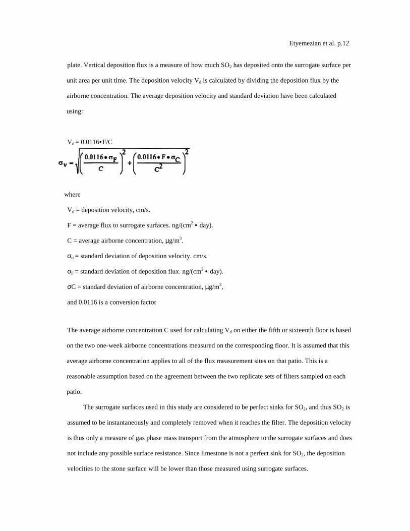
Etyemezian et al. p.12
plate. Vertical deposition flux is a measure of how much SO2 has deposited onto the surrogate surface per
unit area per unit time. The deposition velocity Vd is calculated by dividing the deposition flux by the
airborne concentration. The average deposition velocity and standard deviation have been calculated
using:
Vd = 0.0116•F/C
where
Vd = deposition velocity, cm/s.
F = average flux to surrogate surfaces. ng/(cm2 • day).
C = average airborne concentration, µg/m3.
συ = standard deviation of deposition velocity. cm/s.
σF = standard deviation of deposition flux. ng/(cm2 • day).
σC = standard deviation of airborne concentration, µg/m3,
and 0.0116 is a conversion factor
The average airborne concentration C used for calculating Vd on either the fifth or sixteenth floor is based
on the two one-week airborne concentrations measured on the corresponding floor. It is assumed that this
average airborne concentration applies to all of the flux measurement sites on that patio. This is a
reasonable assumption based on the agreement between the two replicate sets of filters sampled on each
patio.
The surrogate surfaces used in this study are considered to be perfect sinks for SO2, and thus SO2 is
assumed to be instantaneously and completely removed when it reaches the filter. The deposition velocity
is thus only a measure of gas phase mass transport from the atmosphere to the surrogate surfaces and does
not include any possible surface resistance. Since limestone is not a perfect sink for SO2, the deposition
velocities to the stone surface will be lower than those measured using surrogate surfaces.

Etyemezian et al. p.13
6. DISCUSSION
6a. Airborne Concentrations of chemical Species
The airborne concentration data have been analyzed statistically using a two sided t-test for averages.
Significant differences in concentrations among the three sampling locations do not exist for any of
the pollutants considered (Table 4).
The presence of a vertical concentration gradient requires that two conditions hold true.
First, emissions from nearby sources must be sufficiently large to increase pollutant concentrations
above the urban background level. Second, atmospheric mixing must be sufficiently small that
vertical concentration differences can persist.
SO42- and NO3
- particles and HNO3 gas are generally secondary pollutants that form from chemical
reactions in the atmosphere (Seinfeld and Pandis, 1997). Therefore, on spatial scales corresponding
to the height of the Cathedral, airborne concentrations of these species are expected to be spatially
homogeneous since their formation is sufficiently slow to allow mixing, SO42- and No3
- are
sometimes associated with coarse particles, in part due to sorption of SO2 and HNO3 onto alkaline
soil dust (Wolff 1984). The absence of a concentration gradient in S042- particles and total NO3
-
suggests that if these species are associated with coarse particles, there is adequate mixing to
distribute them over the height of the Cathedral. The fact that elemental carbon does not exhibit a
concentration gradient suggests that motor vehicle emissions from adjacent streets and the emissions
from the nearby coal-fired steam plant are either rapidly mixed or else do not contribute significantly
to concentrations at or above the fifth floor.
To investigate the extent of pollutant mixing near the building, a limited number of
measurements of vertical wind speed were conducted on the fifth and sixteenth floor patios on five
days during the term of this project. Results show the presence of strong vertical air motions along
the walls of the building on all days tested. Although preliminary, these results provide qualitative
evidence of vertical mixing as a consequence of wind impinging on the Cathedral. 6b. Laser Particle Counts

Etyemezian et al p.14
In the >0.5 µm size range, particle Counts by LPC do not show a significant difference between the fifth and sixteenth
floors (Figures 7 and 8). However, >5 µm particle counts are on average 30% higher on the sixteenth floor than on the
fifth floor Because of their greater inertia, sampling of large particles is more sensitive to factors such as inlet angle, flow
characteristics in the inlet, and ambient wind direction. Therefore, the discrepancy in >5 µm concentrations between the
two floors should be regarded with caution. Note that the chemical species data do not show a difference between the fifth
and sixteenth floors: if the >5 µm particle concentrations are indeed slightly greater on the sixteenth floor, then it is
unlikely that there is much SO42-. NO3
-, or carbon mass associated with these large particles.
Figures 7 and 8 both demonstrate that particle counts can vary considerably over the course of a day. In Figure 7,
maxima and minima for >0 5 µm particle concentrations coincide well with those for >5 µm particles. This agreement
between concentrations in the two particle sizes is found in most of the LPC data. However, changes in >0 5 µm particle
concentrations are not well proportioned with those of >5 µm particles. The correlation coefficient for the data in Figure
7 is 0.41 whereas the 24-hour based correlation coefficients for all available LPC data range from-0.27 to 0.90 with a
median value of 0.37. The low positive and occasional negative correlations are not surprising. Some meteorological
parameters such as atmospheric stability may qualitatively affect >0 5 µm and >5 µm particle concentrations similarly.
However, particles in these two size ranges are generally not emitted by the same sources and are not subjected to
identical transport processes.
Table 3 shows that concentrations on Saturdays and Sundays are lower than those on weekdays. This is consistent
with the expectation of reduced motor vehicle traffic and, possibly, reduced operations of some stationary sources on
weekends in the Pittsburgh area.
6c. Vertical Deposition Flux and Vertical Deposition Velocities
There is considerable spatial variability in SO2 deposition within each patio. However, most deposition velocities (Vd) are
in the range 0.6-1.0 cm/s which is in agreement with unpublished data obtained previously at the Cathedral (Lutz et al.,
1994; Etyemezian et al., 1995). The values are also in agreement

Etyemezian et al. p.15
with measurements using the same method by Wu et al. (1992) on a bronze equestrian Statue in Gettysburg National
Military Park. The greatest deposition velocities on the sixteenth floor correspond to locations 16a and 16c. The average
deposition velocities for the full year are 0.85 ± 0.13 cm/s for the sixteenth floor compared with 0.69 ± 0.07 cm/s for the
fifth floor. The sampling locations on the sixteenth floor are more exposed than those on the fifth floor which may, in
part, be responsible for the slightly higher deposition velocities. Note that Sites 5a and 5f the most exposed sites on the
fifth floor, have the highest deposition velocities on that floor. It is also of interest that the relative magnitudes of
deposition velocity at one location with respect to another location do not change seasonally. For example, Vd is
consistently higher at location 16c than it is at locations 5b, 5c, 5d, 5e. and 5f. Unpublished results of previous sampling
at the Cathedral show a similar trend for SO42- particle deposition (Gould et al., 1993; Lutz et al., 1994; and Etyemezian
et al., 1995). These data also show that deposition fluxes of SO42- particles to surrogate surfaces are usually at least a
factor often lower than those for SO2. In the earlier studies, surrogate surfaces for SO42- particle and SO2, gas collection
were exposed on the fifth floor at five locations.
Locations 5f, 16a, and l6c are on parts of the building where there is no visible soiling. Location Sa is inside a 0.5 m
heavily soiled indent on the wall. The portion of the wall immediately outside the indent and closer to the outer corner
of the patio is clean. Overall, those sampling locations with the highest deposition velocities correspond to unsoiled
parts of the building surface, and these are in relatively exposed areas. Furthermore, observations of the building during
rainstorms suggest that these exposed areas also experience the most impingement by rain. Thus, we propose that
deposition of pollutants and surface rain washing are processes in dynamic competition.
Archival photographs showing changes in soiling from the 1930’s to the present support this hypothesis. These
photographs show heavy soiling in the early years with decreasing amounts of soiling in more recent times. Examples of
two photographs, from the late 1930’s and from 1995, are shown in Figure II. The first photograph shows extensive
soiling on the southwestern façade. In contrast, the later photograph shows that the top one-third of the building is
virtually free of soiling, and that the demarcation line between soiled and unsoiled surfaces has receded on other parts of
the building. Figure 12 indicates that the amount of annual precipitation has been roughly constant over these decades.
However, airborne concentrations of SO2, and particles have decreased steadily over the same time period (Davidson.
1979).

Etyemezian et al. p.16
Thus, those areas of the façade that were soiled in the late 1930’s have become unsoiled in recent years because the rate
of removal of soiled material by rain washing is greater than the rate of soiling by pollutant deposition and chemical
reaction. The earlier photograph suggests that the opposite was true in the late 1930’s.
A study of the composition of the limestone on the Cathedral of Learning (McGee, 1997) supports the hypothesis that
the soiling is a direct result of pollutant deposition. McGee has collected 37 samples of black, light, and red-brown surface
material for examination by optical microscopy and electron scanning microscopy (SEM) with energy dispersive x-ray
analysis of some samples. The black samples are composed primarily of CaSO4 (gypsum) and contain numerous Fe-. Si-,
and Al-rich fly ash particles. This is attributed to deposition of metal-containing particles and sulfur from pollutant sources
in the area. The light surfaces are primarily calcite with only minor amounts of gypsum and metals. McGee reports that the
microscopic and macroscopic appearance of light samples is similar to that of other limestone samples that are regularly
washed either by rain or by routine cleaning. The color of the red-brown samples is attributed to rust from small metal
spheres lodged in the stone, probably as a result of surface finishing of the limestone block.
It is of interest that one of the rainshields shown in Figure 4 was deployed in a soiled area on the fifth floor patio
in January 1993; since then, the surface of the stone immediately above the rainshield has become cleaned by splashing
raindrops (Figure 13). Clearly, the presence of this rainshield has caused a local disturbance in the balance between
pollutant deposition and surface rain washing and has enhanced the amount of washing.
6d. Applicability of Results to Other Limestone Buildings
The absence of a vertical pollutant concentration gradient is probably due to a combination of factors that have
implications for buildings in other areas. First, it is likely that vertical mixing is enhanced by the presence of the building;
tall buildings in other areas may also have strong upward air motions that can deliver pollutants generated near the ground
to upper levels. Second, the location of pollution sources around the Cathedral can greatly affect the airborne
concentrations at the building. The Cathedral is located

Etyemezian et al. p.17
in a major urban area with considerable local traffic as well as mobile and stationary sources for several kilometers in all
directions. Thus, the contributions from nearby sources (within a few hundred meters) may be diminished by the presence
of numerous regional pollution sources. Note that pollutants from several kilometers away have time to mix vertically in
the atmosphere and can increase airborne concentrations at higher elevations. Effects of nearby sources may be more
pronounced in cases where a building is located in a less polluted setting.
Third, the presence of nearby buildings is likely to have a major effect on dispersion near any building. The
Cathedral is considerably taller than the surrounding buildings, and is 80 m from the nearest buildings to the north and
west and over 120 m from the nearest buildings to the south and east. This isolation eliminates some of the trapping of
pollutants that may occur in narrow street canyons, as reported by Lee and Park (1994).
It must be noted that no measurements in the present study were conducted below the fifth floor, and thus
conclusions regarding the absence of a concentration gradient apply only above this level.
The concept of pollutant deposition and rain washing as competing processes has implications for other buildings.
Comparing modem and archival photographs of the Cathedral shows general decreases in the soiling that are qualitatively
consistent with decreases in pollutant concentration. Archival photographs of buildings where soiling is due to microbial
activity may show distinctly different patterns.
7. SUMMARY AND CONCLUSIONS
In order to better understand pollutant sources and transport pathways responsible for the soiling of a tall limestone
building, this study has investigated whether vertical gradients in airborne pollutant concentrations and deposition fluxes
currently exist at the 42-story Cathedral of Learning in Pittsburgh, PA. The study has also considered long-term changes in
soiling on the building as a means of identifying the roles of pollutant deposition and rain washing in affecting the soiling
patterns.
The study involved measurements of airborne concentrations of SO42- particles, elemental carbon particles. SO2 gas,
and total NO3- (NO3
-; particles and HNO3 gas) on the fifth floor, sixteenth floor, and roof. In addition. SO2 deposition
fluxes were measured on the fifth and sixteenth floors, and laser particle

Etyemezian et al p.18
counters were used on these same two floors to measure airborne particle number concentrations in two size ranges: >0.5
µm and >5 µm. The experiments were conducted for four weeks during each of the four seasons of the year beginning in
fall 1995.
The airborne chemical species measurements indicate that there are no statistically significant vertical
gradients for any of the pollutants. The lack of a gradient is attributed to a variety of regional and local sources that are
expected to be well mixed by the time they reach the Cathedral, vertical winds in the vicinity of the building, and the lack
of buildings nearby that might otherwise trap pollutants and prevent vertical mixing. The laser particle counts for >0.5
µm particles likewise show lack of gradient, although the >5 µm particles show slightly greater airborne particle number
concentrations on the sixteenth floor compared with those on the fifth floor.
Deposition fluxes and deposition velocities of SO2 to surrogate surfaces show small but consistent
differences among the locations sampled. Values are greatest at locations that are most exposed to the wind such as the
outside corners of the patios. The values are greater on the sixteenth floor than on the fifth floor, partly because two of
the three sixteenth floor sampling locations are situated on the corners of the patio.
Comparison of archival with more recent photographs shows that the soiling on the Cathedral has decreased
over time. This is consistent with decreasing trends in airborne pollutant concentrations over the past several decades. It
is thus likely that rain is washing soiled material off the building surface at a greater rate than chemical species are
depositing and reacting with the surface. The opposite apparently was true in the 1930’s when air pollutant
concentrations were considerably greater than at present.
Overall, these results may be of interest to conservators who must develop strategies for cleaning and
restoring building surfaces and for preventing future damage. Although the conclusions reached here are a result of
testing at the Cathedral of Learning, it is likely that many of the findings also apply to buildings in other urban areas.
8. ACKNOWLEDGMENTS
This research was funded by the National Park Service Cooperative Agreements 042419005 and 00196035.
The assistance of the Department of Facilities Management at the University of Pittsburgh and Dominic

Etyemezian et al p.19
Fagnelli, the Cathedral of Learning building engineer, are greatly appreciated. The authors wish to acknowledge Susan
Sherwood for her valuable suggestions and assistance over the past several years. Thanks are due to Michael Lutz and
Timothy Gould for their earlier work on the Cathedral and to Mitchell Small for help with the statistical analysis. The
authors also wish to thank Spyros Pandis, Hampden Kuhns, Weiping Dai, Maria Zufall, and Ross Strader for their frequent
and welcome suggestions. Chandra Reedy and Elizabeth Bede provided comments and insights that were very helpful in
the writing of this manuscript. A large fraction of the airborne sampling setup was constructed by Larry Cartwright and his
crew. Karen Pinkston and Preshanth Mekala contributed their time to ion chromatography analyses. The historical
photograph was furnished by the Carnegie Library of Pittsburgh, Oakland Branch. Justin Parkhurst assisted with the
collection of several historical photographs. The computer drawings of the Cathedral that appear in Figure 2 were created
by Judy Lee and modified by Ivan Locke, Sean Jutahkiti, Anthony Paul, and Thomas Curry are thanked for their work on
measuring vertical wind speeds near the walls of the Cathedral of Learning.
9. REFERENCES
Amoroso, G.G., and V. Fassina. 1983. Stone Decay and Conservation: Atmospheric Pollution, Cleaning, Consolidation
and Protection. Materials Science Monographs 11, Elsevier, 1983.
Appel, B.R., Y. Tokiwa, and M. Haik. 1981. Sampling of Nitrates in Ambient Air. Atmospheric Environment 15: 283-289.
Bock, E. and W. Sand. 1993. A Review: The Microbiology of Masonry Deterioration .Journal of Applied
Bacteriology 74: 503-514.
Braun, R.C., and M.J.G. Wilson. 1970. The Removal of Atmospheric Sulphur by Building Stones.
.Atmospheric Environment 4: 371-378.

Etyemezian et al p.20
Cadle, S.H., and P..A. Mulawa. 1987. The Retention of SO2 by Nylon Filters. Atmospheric Environment 21:
599-603.
Chan, W.H., D.B. Orr, and D.H.S. Chung. 1986. An Evaluation of Artifact SO42- Formation on Nylon Filters
Under Field Conditions. Atmospheric Environment 20: 2397-2401.
Chow, J.C., J.G. Watson, L.C. Pritchet, W.R. Pierson, C..A. Frazier, and R.G. Purcell. 1993. The DR.I
Thermal/Optical Reflectance Carbon Analysis System: Description, Evaluation, and Applications in U.S.
Air Quality Studies. Atmospheric Environment 27a: 1185-1201.
Dabberdt, W.F., and W.G. Hoydysh. 1991. Street Canyon Dispersion: Sensitivity to Block Shape and
Entrainment. Atmospheric Environment 25a: 1143-1153.
Davidson. C.I. 1979. Air Pollution in Pittsburgh: A Historical Perspective. Journal of the Air Pollution
Control Association 29: 1035-1041.
Davidson. C.I., S.E. Lindberg. J.A. Schmidt, L.G. Cartwright, and L.R. Landis. 1985. Dry Deposition of Sulfate
Onto Surrogate Surfaces. Journal of Geophysical Research 90:. 2123-2130.
Del Monte. M., C. Sabbioni, and O. Vittori, 1981. Airborne Carbon Particles and Marble Deterioration.
Atmospheric Environment 15: 645-652.
DePaul, F.T., and C..M. Sheih. 1986. Measurements of Wind Velocities in a Street Canyon. Atmospheric
Environment 20: 455-459.
Etyemezian, V., C.I. Davidson, S. Finger et al. 1995. Influence of Atmospheric Pollutants on Soiling of a
Limestone Building Surface. Progress Report for the National Park Service. September, 1995.

Etyemezian et al. p.21
Fenter, F.F., C. Francois, and M..J. Rossi. 1995. Experimental Evidence for the Efficient “Dry Deposition” of
Nitric Acid on Calcite. Atmospheric Environmental 29: 3365-3372.
Freemantle, M. 1996. Historic Monuments Pose Challenge to Conservation Scientists. Chemical and
Engineering News 74: 20-23.
Gould, T.R., C.I. Davidson, S. Finger et al. 1993. Influence of Atmospheric Pollutant Concentrations and
Deposition Rates on Soiling of a Limestone Building Surface Progress Report for the National Park
Service. May, 1993.
Haneef, S.J., J..B. Johnson, C. Dickinson, G.E. Thompson, and G.C. Wood. 1992. Effect of Dry Deposition of
NOx and SO2 Gaseous Pollutants on the Degradation of Calcareous Building Stones Atmospheric Environment
26a: 2963-2974.
Hering, S.V. et al. 1988. The Nitric Acid Shootout Field Comparison of Measurement Methods.
Atmospheric Environment 22: 1519-1539.
Hoydysh, W G., and W..F. Dabberdt. 1994. Concentration Fields at Urban Intersections: Fluid Modeling Studies.
Atmospheric Environment 28: 1849-1860.
Huber, A.H., S. Pal Arya, S.A. Rajala, and J.W. Borek. 1991. Preliminary Studies of Video Images of Smoke
Dispersion in the Near Wake of a Model Building. Atmospheric Environment 25a: 1199-1209.
Hutchinson, A.J., J.B. Johnson, G.E. Thompson. G. C. Wood. P.W. Sage, and M.J. Cooke. 1992. The Role of Fly-
ash Particulate Material and Oxide Catalysts in Stone Degradation. Atmospheric Environment 26a:
2795-2803.

Etyemezian et al. p.22
Hutchinson, A.J., J.B. Johnson, G.E. Thompson, G.C. Wood, P.W. Sage, and M.J. Cooke. 1993. Stone
Degradation Due to Wet Deposition of Pollutants. Corrosion Science 34: 1881-1898.
Johansson. L.G., O. Lindqvist, and R.E. Mangio. 1988. Corrosion of Calcareous Stones in Humid Air Containing
SO2 and NO2. Durability of Building Materials 5: 439-449.
Judeikis, H.S., T.B. Stewart, and A.G. Wren. 1978. Laboratory Studies of Heterogeneous Reactions of SO2.
Atmospheric Environment 12: 1633-1641.
Kirkitsos, P., and D. Sikiotis. 1995. Deterioration of Pentelic Marble, Portland Limestone and Baumberger
Sandstone in Laboratory Exposures to Gaseous Nitric Acid. Atmospheric Environment 29: 77-86.
Lee, J.T., D.L. Call, R.E Lawson Jr., W.E. Clements, and D.E. Hoard. 1991. A Video Image Analysis
System for Concentration Measurements and Flow Visualization in Building Wakes. Atmospheric
Environment 25a: 1211-1225.
Lee, I.Y., and H.M. Park. 1994. Parametrization of the Pollutant Transport and Dispersion in Urban Street
Canyons. Atmospheric Environment 28: 2343-2349.
Livingston, R.A. 1992. Graphical Methods for Examining the Effects of Acid Rain and Sulfur Dioxide on
Carbonate Stones. Proceedings of the 7th International Congress on Deterioration and Conservation of
Stone. Lisbon, Portugal. 1992. 375-386.
Lutz, M.R., C.I. Davidson, S. Finger et al. 1994. Influence of Atmospheric Pollutants on Soiling of a Limestone
Building Surface 1991-1994. Progress Report for the National Park Service. September, 1994.
McGee, E.S. 1995. Sampling Protocol Used at the Cathedral of Learning in Pittsburgh, Pennsylvania.
USGS Open-File Report 95-672.

Etyemezian et al. p.23
McGee, E.S. 1997. Surficial Alteration at the Cathedral of Learning in Pittsburgh, Pennsylvania. USGS
Open-File Report 97-275.
Meierding, T.C. 1993. Marble Tombstone Weathering and Air Pollution in North America. Annals of the
Association ofAnierican Geographers 83 (4): 568-588.
Mitchell, J D. Gu.R., T.E. Ford, and N.S. Berke. 1996. Fungal Degradation of Concrete. DECHEMA
Monographs 133: 135-142.
Mossotti, V.G., and A.R. Eldeeb. 1994. Calcareous Stone Dissolution by Acid Rain. Manuscript in progress.
Version-0.7, Dec. 12, 1994.
Mulawa, P.A., and S.H. Cadle. 1985. A Comparison of Nitric Acid and Particulate Nitrate Measurements by the
Penetration and Denuder Difference Methods. Atmospheric Environment 19: 1317-1324.
Palmer et al. 1991 as cited in Bock and Sand (1993). Palmer, R.J., J. Siebert, and P. Hirsch 1991. Biomass and
Organic Acids in Sandstone of a Weathering Building: Production by Bacterial and Fungal Isolates.
Microbial Ecology 21: 253-266.
Qin, Y., and S.C. Kot. 1990. Validation of Computer Modeling of Vehicular Exhaust Dispersion Near a Tower
Block. Building and Environment 25: 125-131.
Qin, Y., and L.Y. Chan. 1993. Traffic Source Emission and Street Level Air Pollution in Urban Areas of
Guangzhou, South China (P.R.C.). Atmospheric Environment 27b: 275-282.
Qin, Y., and S.C. Kot 1993. Dispersion of Vehicular Emission in Street Canyons, Guangzhou City, South China
(P.R C.). Atmospheric Environment 27b: 283-291.

Etyemezian et al. p.24
Sabbioni, C. 1994. Effects of Air Pollution on Historic Buildings and Monuments. Scientific Basis for
Conservation: Physical. Chemical, and Biological Weathering. European Cultural Heritage Newsletter on
Research 8(1): 2-6.
Seinfeld, J.H., and S.N. Pandis. 1997. Atmospheric Chemistry Air Pollution to Global Change. John Wiley and Sons,
1997 (in press).
Sherwood, S.I., D.A. Gatz, R.P. Hosker Jr. et al. 1990. Processes of Deposition to Structures. NAPAP SOS/T Report
20 in National Acid Precipitation Assessment Program. Acidic Deposition: State of Science and Technology. Volume
III. September 1990.
Spedding, D.J. 1969. Sulphur Dioxide Uptake by Limestone. Atmospheric Environment 3: 683.
Spiker, E.C., R.P. Hosker Jr., V.C. Weintraub, and S.I. Sherwood. 1995. Laboratory Study of SO2 Dry
Deposition on Limestone and Marble: Effects of Humidity and Surface Variables. Water, Air, and Soil
Pollution Proceedings of the 1995 5th International conference on Acidic Deposition: Science and Policy.
Acid Reign 95, Goteberg, Sweden. 1995. 2679-2685.
Tayler, S., and E. May 1991. The Seasonality of Heterotrophic Bacteria on Sandstones from Ancient
Monuments. In Biodeterioration of Cultural Property ed. R.J. Koestler, Elsevier, New York, NY. 390-391.
Thompson, R.S. 1993. Building Amplification Factors for Sources Near Buildings:A Wind Tunnel Study.
Atmospheric Environment 27a: 2313-2325.
Warscheid, T., M. Oelting, and W.E. Krumbein. (1991). Physico-chemical Aspects of Biodeterioration
Processes on Rocks with Special Regard to Organic Pollutants. In Biodeterioration of Cultural Property ed.
R.J. Koestler, Elsevier, New York. NY. 397-399.

Etyemezian et al p.25
Wilmzig, M., and E. Bock 1995. Endangerment of Mortars by Nitrifiers, Heterotrophic Bacteria and Fungi.
In Biodeterioration and Biodegradation 9 eds. A. Bousher et al., Institution of Chemical Engineers, Rugby,
UK, 195-197.
Winkler, E.M. 1996. Important Agents of Weathering for Building and Monumental Stone. Engineering
Geology 1:381-400.
Wolff, G.T. 1984. On the Nature of Nitrate in Coarse Continental Aerosols Atmospheric Environment 18:
977-981.
Wu, Y.L., C.I. Davidson, D.A Dolske, and S.I. Sherwood. 1992. Dry Deposition of Atmospheric
Contaminants:The Relative Importance of Aerodynamic, Boundary Layer, and Surface Resistances.
Aerosol Science and Technology 16: 65-81.
Young, P. 1996a. Pollution-Fueled “Biodeterioration” Threatens Historic Stone Environmental Science
and Technology 30: 206a-208a.
Young, P. l996b. Mouldering Monuments. New Scientist 152: 37-38.
Zappia, G., C. Sabbioni, and G. Gobbi. 1993. Non-Carbonate Carbon Content on Black and White Areas of Damaged
Stone Monuments. Atmospheric Environment 27a: 1117-1121.

Etyemezian et al. p.26
10. SUPPLIERS OF EQUIPMENT
1. Clean Room Products Inc., 1800 Ocean Avenue, Ronkonkoma, NY 11779-6532.
2. Costar, One Alewife Center, Cambridge, MA 02140.
3. Dionex Corp., 1228 Titan Way, Sunnyvale, CA 94088-3603. 4. Fisher Scientific, 711 Forbes Avenue, Pittsburgh, PA 15219-4785.
5. Gelman Sciences, 600 South Wagner Road, Ann Arbor, MI 48106.
6. Hoke, One Tenakill Park, Cresskill, NJ 07626.
7. Millipore Corp., 80 Ashby Road, Bedford, MA 01730.
8. Pallflex Corp., 125 Kennedy Drive, Putnam, CT 06260.
9. Savillex Corp., 6133 Baker Road, Minnetonka, MN 55345.
10. Singer Corp., product division closed.
11. TSI Inc., P.O. Box 64394, St Paul, MN 55164.
12. Whatman, 9 Bridgewell Place, Clifton, NJ 07014.

Etyemezian et al. p.27
11. AUTHOR BIOGRAPHIES
Vicken Etyeinezian is a doctoral student at Carnegie Mellon University (CMU). He received combined bachelor degrees in
physics and engineering from Occidental College and Caltech, respectively and an MSE in environmental engineering from the
Johns Hopkins University. His research has focused on the effects of atmospheric pollutants on sensitive building materials, with
an emphasis on dry deposition and surface rain washing. Some of his other interests include policies for sustainable
environments in developing countries, urban and remote atmospheric chemistry, contaminant transport in groundwater, and
innovative solutions for wastewater treatment.
Cliff I. Davidson is Professor of Civil and Environmental Engineering/Engineering and Public Policy at Carnegie Mellon
University (CMU). He is also Director of the Environmental Institute at CMU. His main research interests involve atmospheric
pollutants, focusing on the way particles and gases are transported through the atmosphere, the mechanisms by which particles
and gases deposit from the atmosphere onto different types of surfaces, and historical trends in air pollution levels. His main
educational activities include developing material that can be used broadly in basic science and engineering courses to increase
student awareness of environmental issues.
Susan Finger is on the faculty of the Civil and Environmental Engineering Department at Carnegie Mellon University. She is
also affiliated with the Engineering Design Research Center, the Robotics Institute, and the Department of Mechanical
Engineering. She is a founder and Co-Editor-in-Chief of the journal Research in Engineering Design. Dr. Finger’s research
interests include representation languages for designs, integration of design and manufacturing concerns and computer-aided
engineering.
Barabas Noemi received a BS degree in chemical engineering and public policy with a minor in environmental engineering from
Carnegie Mellon University. She is completing work on a master’s degree (with subsequent Ph.D.) in Environmental
Engineering in the Water Resources and Environmental

Etyemezian et al p.28
Engineering Program at the University of Michigan. Her interests are water resource management and policy and its application
in Eastern Europe.
Mary F. Striegel currendy serves as the Materials Research Program Coordinator for the National Center for Preservation
Technology and Training, where she is responsible for the supervision of in-house and external research on the effects of air
pollution on cultural resources. Before coming to NCPTT, Mary was a researcher with the Getty Conservation Institute. She
holds bachelor degrees in fine arts and chemistry from the University of Louisville, a masters degree in analytical chemistry
from Indiana University-Purdue University in Indianapolis, and a doctoral degree in inorganic chemistry from Washington
University in St. Louis.
Dr. Judith C. Chow, Research Professor in the Energy and Environmental Engineering Center (EEEC) at the Desert Research
Institute (DRJ). University and Community College System of Nevada, has over 19 years of experience in conducting air quality
studies and performing statistical data analysis. She directs DRI’s Environmental Analysis Facility where she supervises filter
processing and chemical operations. In this capacity, she has developed cost-effective, yet accurate, methods for sampling and
analysis. Dr. Chow has gained extensive experience in program planning: ambient and source sampling from urban and non-
urban areas; gravimetric, x-ray fluorescence, atomic absorption spectrophotometric, ion chromnatographic, automated
colorimetric, and thermal/optical reflectance carbon analyses of filter samples, as well as interpretative statistical data analyses,
principal component analyses, such as multivariate statistical analysis, and chemical mass balance receptor modeling: data
interpretation: and reporting.

Etyemezian et al. p.29
12. LIST OF TABLES
Table 1. Sampling Schedule at The Cathedral of Learning a.
Table 2. Analytical Detection Limits. Average Sample Mass and Average Field Blank Mass.
Table 3. Weekday, Saturday, and Sunday Average Particle Concentrations.
The first and last days of a sampling period are not included in particle concentration averages.
Table 4. P-Values for Two Sided t-tests of Sample Mean for Chemical Species Airborne Concentrations a

Etyeniezian et al. p.30
13. LIST OF FIGURES
Figure 1. Location Map Centered at the Cathedral of Learning.
Enlarged from 7.5 minute by 7.5 minute USGS map (1969).
Figure 2. Sampling Sites at the Cathedral of Learning.
Figure 3a. Wind Direction Occurrence Frequency.
Markers indicate the fraction of time wind is blowing from the indicated direction during the sampling periods:
11/20/95-12/18/95, 2/1/96-2/29/96, and 5/14/96-6/12/96. Data were not available for the 7/24/96-8/21/96 sampling
period. Measurements were made at the AGC Meteorological station 10 km south of the Cathedral of Learning Data
were obtained from the National Climatic Data Center Web page
Figure 3b. Wind Speed Occurrence.
Markers indicate the average wind speed (meters per second) when the wind is blowing from the indicated direction
during sampling periods: 11/20/95-12/18/95, 2/1/96-2/29/96, and 5/14/96-6/12/96. Data were not available for the
7/24/96-8/21/96 sampling period Measurements were made at the AGC Meteorological station 10 km south of the
Cathedral of Learning. Data were obtained from the National Climatic Data Center Web page.
Figure 4. Schematic of a Vertical Deposition Sheet and Rainshield.
Figure 5. Concentrations Averaged Over All Four Seasons.
Figure 6. Seasonal Concentrations Averaged Over the Three Sampling Locations.
Figure 7a. Laser Particle Counts for >0.5 µrn Particles 2/16/96-2/21/96.
Major and minor tick marks correspond to midnight and noon of indicated date, respectively. Data have been averaged
over ten minutes for legibility
Figure 7b. Laser Particle Counts for >5 µm Particles 2/16/96-2/21/96.
Major and minor tick marks correspond to midnight and noon of indicated date, respectively. Data have been averaged
over ten minutes for legibility.

Etyemezian et al. p.31
Figure 8a. Daily Average, Maximum, and Minimum Laser Particle Counts for> 0.5 µrn Particles.
Maxima on 2/21.2/22,2/23,2/27/96 are 107, 133, 146, 109 particles/cm3, respectively. Minima on 2/24,
5/27, 5/29, and 7/26/96 are 0.90, 0.66, 0.97, and 0 86 particles/cm3, respectively Vertical bars extend from
minimum to maximum measured concentrations.
Figure 8b. Daily Average. Maximum, and Minimum Laser Particle Counts for> 5 urn Particles.
Maxima on 2/21,2/22.,2/23,2/27, and 8/13/96 are 1.38, 10.01,20.35, 1.33, and 3.78 particles/cm3,
respectively. Vertical bars extend from minimum to maximum measured concentrations.
Figure 9. SO2 Deposition fluxes.
Figure 10. SO2 Deposition Velocities.
Figure 11. The Cathedral of Learning 1930’s and Present.
The photograph on the left was taken C, late 1930’s (courtesy of the Carnegie Library of Pittsburgh, Oakland
Branch. Pittsburgh, PA) whereas the photograph on the right was taken in 1995. A comparison of the areas
within the circles illustrates how surface soiling at some locations on the building has decreased. This soiling
is due to deposition and chemical reaction of air pollutants on the limestone surface.
Figure 12. Annual Precipitation for Pittsburgh.
The numbers on the x-axis represent the middle year of the ten year period used to obtain the average annual
precipitation shown Data were obtained from the National Climatic Data Center Web page.
Figure 13. Washing of a Soiled Surface at the Cathedral by Raindrops Impinging on a Rainshield.
The rainshield shown was mounted on the wall of the Cathedral in January 1993. The photograph above was
taken in September 1997. The portion of the wall above the rainshield has been cleaned by raindrops
impinging on the top surface of the rainshield.

Table 1. Etyemezian et al.
a A vertical line indicates a sample change. b No data past 8/16/96

Table 2. Eyemezian et al. Filter Type Analytea Analytical
detection limit(µµµµg on filter)
Average sample mass
(µµµµg)
Average FieldBlank mass
(µµµµ&g) Teflon NO3
- 0.2 18.9 0.92 SO4
2- 0.2 56.2 0.43 Nylon NO3
- 0.2 28.0 0.47 SO4
2- 0.2 19.2 0.59 Cellulose SO4
2- 0.9 284 1.4 Cellulose Backup SO4
2- 0.9 20.9b 1.0 Quartz Elemental Carbon 0.6 70.5 0.30 Cellulose Vertical SO4
2- 0.9 2830 2.5 a Teflon filters collected NO3
- and SO42- particles, while nylon filters collected HNO3 and small amounts of SO2.
Cellulose filters collected SO2. b Average excludes Backup filters that were not found to be different from the blank at 95% confidence

Table 3. Etyemezian et al.
Sampling Period Average concentrations of >0.5 µµµµm particles
(particles/cm3)
Average concentrations of >5 µµµµm particles x 100
(particles/cm3) Weekdays Saturdays Sundays Weekdays Saturdays Sundays
2/8/96 - 2/29/96 24.1 14.4 5.2 8.86 0.68 0.76 5/22196 - 6/12/96 14.2 11.7 7.9 1.02 0.75 0.36 7/24/96 - 8/16/96 23.5 12.8 14.6 0.50 0.39 0.29

Table 4 Etvemezian et al
Chemical Species P-values for 5th floor and 16th floor
P-values for 5th floor and roof
P-values for 16th floor and roof
SO42- 0.953 0.993 0.959
total NO3- 0.981 0.478 0.500
SO2 0.375 0.539 0.895 Elemental carbon 0.897 0.518 0.451 a In order for two sets of data to have significantly different mean values (in a statistical sense), the P-value has to be lower than unity minus the confidence of the test. For example, to show that mean concentrations for a chemical species on the 5th floor are different than those on the 16th floor with 95% confidence, the P value would have to be less than 0.05 (1-0.95).

Figure 1. Etyemezian et al.

Figure 2. Etyemezian et al.
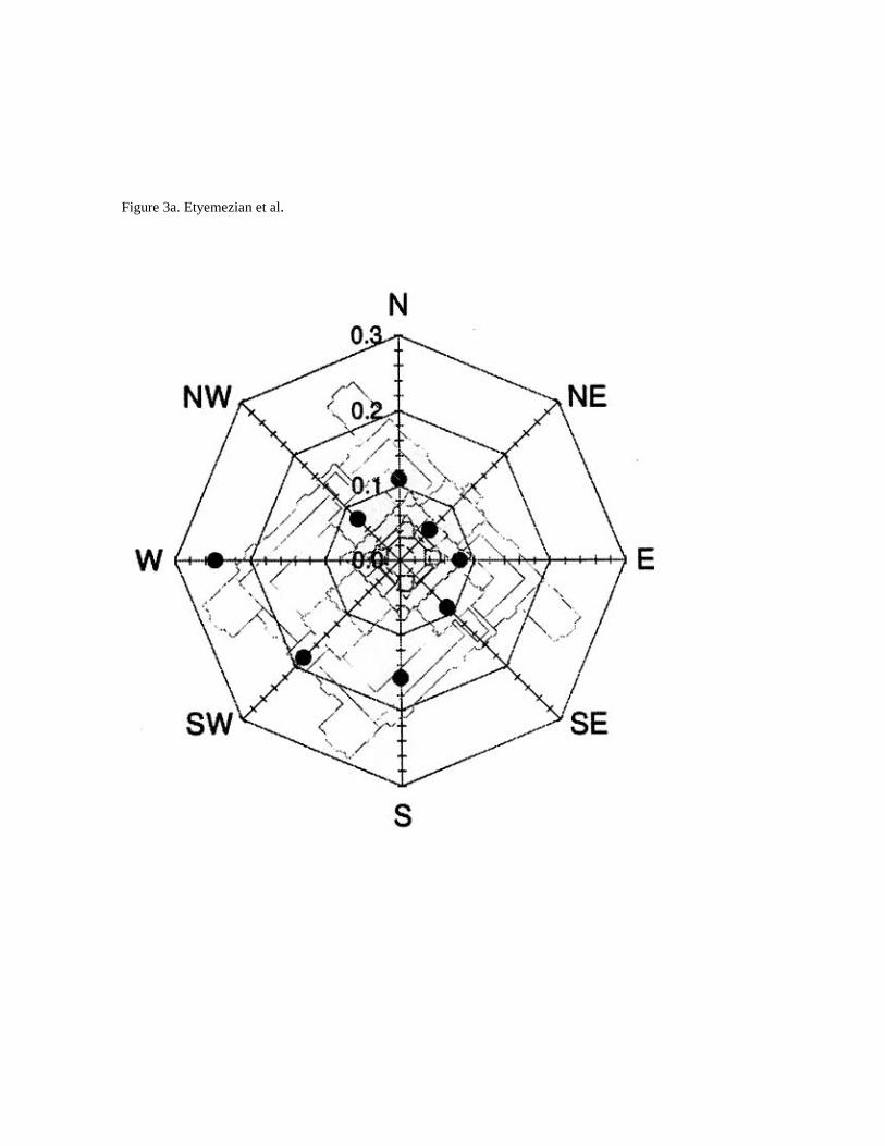
Figure 3a. Etyemezian et al.

Figure 3b. Etyemezian et al.

Figure 4. Etyemezian et al.
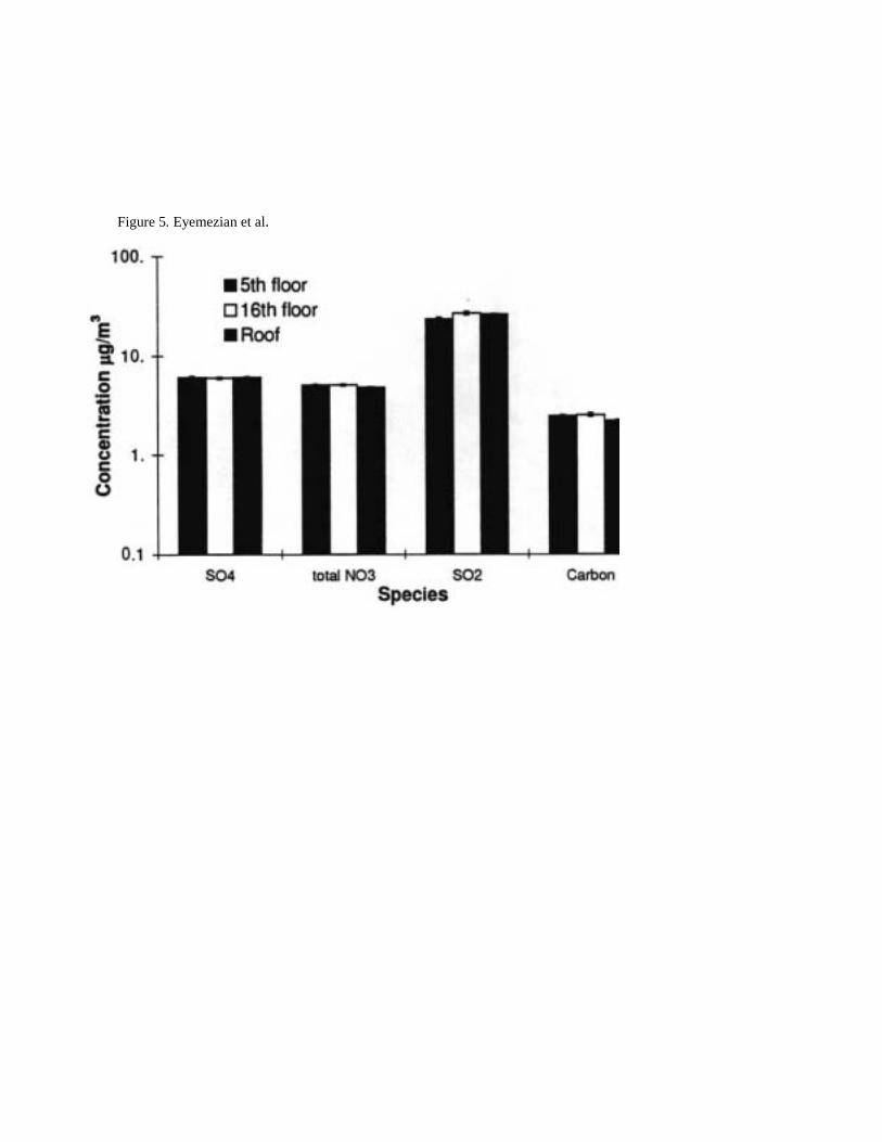
Figure 5. Eyemezian et al.

Figure 6. Etyemezian et al.

Figure 7a. Etyemezian et al.

Figure 7b. Etyemezian et al.

Figure 8a. Etyemezian et al

Figure 8b. Etyemezian et al.

Figure 9. Etyemezian et al.

Figure 10. Etyemezian et al

Figure 11. Etyemezian et al.

Figure 12. Etyemezian et al.
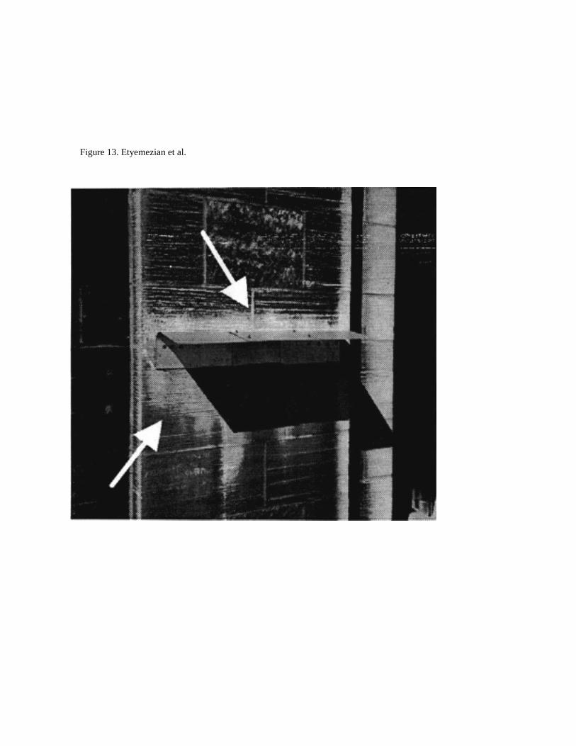
Figure 13. Etyemezian et al.