Physical Activity, Present Bias, and Habit Formation

Department of Economics Working Paper Series

Physical Activity, Present Bias, and Habit Formation: Theory and Evidence from Longitudinal Data Brad Humphreys, Jane Ruseski and Li Zhou

Working Paper No. 15-36

This paper can be found at the College of Business and Economics Working Paper Series homepage:

http://be.wvu.edu/phd_economics/working-papers.htm

Physical Activity, Present Bias, and Habit Formation: Theory and

Evidence From Longitudinal Data

Brad R. Humphreys∗

West Virginia University

Jane E. Ruseski†

West Virginia University

Li Zhou‡

University of Alberta

August 2015

Abstract

We investigate temporal decisions to participate in exercise in a dynamic model featuring present bias

and habit formation. The model highlights naivete about present bias and projection bias about habit

formation/decay and implies that promoting participation in physical activity must both encourage the

inactive to start and discourage the active from quitting as behavioral biases apply to both. Our empirical

analysis using data from the British Household Panel Survey (BHPS) develops evidence consistent with

predictions about present bias and habit formation/decay and an interesting asymmetry between starting

and quitting that furthers understanding of existing empirical evidence.

JEL Codes: D1, I12, L83

Key Words: present-bias, physical activity, habit formation, habit decay, projection bias

∗We thank Botond Koszegi and other participants at the 2015 Tsinghua Conference on Theoretical & Behavioral Economics

and the 2015 2nd Workshop on Behavioural and Experimental Health Economics at McMaster University for comments and

suggestions, and Filmer Chu for helping us get access to the British Household Panel data. Department of Economics, College

of Business and Economics, PO Box 6025, Morgantown WV 26506-6025; email: [email protected]; phone: 304-293-

7871.†Department of Economics, College of Business and Economics, PO Box 6025, Morgantown WV 26506-6025; email:

[email protected]; phone: 304-293-7835.‡Department of Economics, 8-14 Tory, Edmonton, AB T6G 2H4 Canada; email: [email protected]; phone: 780-492-4133.

1

1 Introduction

Promoting regular physical activity and reducing disparities in physical activity represents an important

public policy priority because of the many health benefits associated with regular physical activity. Physically

active people are less likely to be obese and less likely to suffer from chronic health conditions like diabetes,

high blood pressure, heart disease and cancer. Further, preventing obesity in part through regular physical

activity is important because once obese, the probability of returning to a healthy weight is low (Fildes

et al., 2015). Despite all we know about the health benefits of physical activity, and numerous campaigns

to promote it, many people still do not engage in the recommended levels of physical activity to achieve

sustainable health benefits. Participation in physical activity, like many other health behaviors, is episodic.

Some people exercise regularly, while others do not. Some people begin to exercise regularly but then stop

and start again. An improved understanding of patterns in physical activity behavior over time may help to

design and implement more effective policies aimed at promoting physical activity.

This paper is inspired by the literature on consumers’ choice of health club contracts and attendance

decisions. DellaVigna and Malmendier (2006), and Garon et al. (2013) find evidence of over-confidence in

future health club attendance consistent with consumers’ naivete about their own present bias. Charness and

Gneezy (2009) and Acland and Levy (2015) find evidence of post-intervention effects of paying subjects to

exercise at health clubs consistent with habit formation. In addition, Acland and Levy (2015) find evidence

of naivete with respect to present bias and projection bias with respect to habit formation. These studies

significantly advanced our understanding of behavioral patterns in gym and health club attendance.

Whether and how these findings can be generalized to the broader area of individual participation in

physical activity are important questions for extending this literature. We assess this in two ways. First,

whether decisions about gym or health club attendance can be generalized to other forms of leisure time

participation in physical activity, such as walking for exercise, going for a jog or run, or exercising in the

home. Second, whether the behavioral patterns observed in the special subject groups used in these studies

can be extended to a more general population.1 The objective of this research is to develop and empirically

test a dynamic model of participation in physical activity that features the behavioral patterns identified

by the gym attendance literature, and to test the predictions of this model using data from a nationally

representative survey.

Our theoretical model builds on dynamic inconsistency models developed by O’Donoghue and Rabin

(1999b) and includes habit formation (Becker and Murphy (1988)) and projection bias (Loewenstein et al.

(2003)). Our model abstracts from the contracting aspects associated with health club membership and

attendance emphasized in the models developed by DellaVigna and Malmendier (2006) and Acland and

1The subjects in Acland and Levy (2015)’s study are students and staff of the University of California, Berkeley. Charness

and Gneezy (2009) study students from the University of Chicago and University of California, San Diego. DellaVigna and

Malmendier (2006) study members of three health clubs in New England and Garon et al. (2013) study members at 14 health

clubs in Quebec.

2

Levy (2013) to focus on decisions about participating in general leisure time physical activity. Physical

activity is modeled as a task with immediate costs, in terms of money, time, effort, and psychic costs2

and delayed rewards, in terms of benefits associated with improved health and weight loss. The habit of

participation in physical activity is a binary state variable (O’Donoghue and Rabin (1999a) and Acland and

Levy (2013)): people who enter a period with the habit of participation in physical activity will face a lower

effort cost of participation in the current period than people who enter without the habit. The habit of

participation is defined by participation in the period immediately before the current period, which means

that the model implicitly includes habit decay. The model also includes conventional economic motivations

such as monetary and time costs associated with participation emphasized by Humphreys and Ruseski (2011)

and a stochastic period-specific participation cost shock.

The theoretical model yields a rich set of predictions on temporal decisions about participation in physical

activity. Predictions regarding naivete and projection bias are not directly testable with secondary data that

have no information on individuals’ ex ante “prediction/perception” of own behavior. The British Household

Panel Survey (BHPS), the data we use for our empirical analysis, unfortunately does not contain such

information. However, the BHPS are rich enough to test other predictions, including the role of present bias

and habit formation (and decay) in physical activity participation. The BHPS is a nationally representative

longitudinal sample of households residing in England, Scotland, Wales and Northern Ireland. This survey

began in 1991 and has been surveying participants annually since. BHPS participants are contacted annually

and asked a comprehensive set of questions on topics ranging from employment status and wages and income

to health status and education. We document participation in physical activity using data from waves 10

(2000), 12 (2002), 14 (2004) and 16 (2006) of the BHPS which included questions about the frequency of

participation in physical activity.

When direct measures of individuals’ time preference are not available, the critical aspect of empirically

testing the negative impact of present bias on physical activity participation lies in finding a reasonable proxy

for present bias. Studies that link directly elicited time preference measures to individual outcomes have

found significant correlation between present bias and smoking (Burks et al. (2012), Grignon (2009) and Kang

and Ikeda (2013)) and accumulation of credit card debt (Meier and Sprenger (2010)). We use information

from the BHPS to construct proxy variables for present bias using responses to questions about past smoking

and accumulation of credit card debt. We find that the probability of starting and continue to participate in

physical activity in later periods (2002, 2004, and 2006) was negatively correlated with smoking in 2000 and

the accumulation of credit card debt by 2000. The probability of quitting participating in physical activity

was positively correlated with smoking in 2000 but not with the accumulation of credit card debt by 2000.

Overall, these results, when combined with findings from the time preference literature, support the idea

that present bias negatively affects participation in physical activity in the general population.

2The model allows negative effort and psychic costs. For people with negative effort costs, they actually enjoy physical

activity and participate not just for the health benefits but also for the enjoyment.

3

The difficulty in empirically testing the role of habituation in decisions to participate in physical activity

using secondary data is endogeneity. An observed correlation between past participation and current partic-

ipation can purely reflect unobserved personal traits or learning about physical activity through experience.

We explore individuals’ past participation history in different ways to test these two alternative hypotheses.

First, we estimate the impact of participation in 2000, 2002, and 2004 on the probability of participation

in 2006. If there is no effect of habit formation and decay and past participation is correlated with cur-

rent participation through time-invariant unobservable personal traits, then the coefficient on the three past

participation variables should be the same. We find that all three coefficients are positive and significantly

different from each other: the coefficients of past participation decline with the time between the current

period and the past participation period, favoring habit formation and decay. Second, we limit our sample to

individuals who participated in physical activity in 2000 and 2002 who may have gone through the learning

process before 2004. We find that, for this group with a relative long history of past participation, partici-

pation in 2004 significantly increases their probability of participation in 2006. This result is consistent with

habit formation and decay and against learning unless learning is slow and takes more than 4 years.

Our empirical analysis also uncovers an interesting asymmetric impact of major events on quitting and

starting participation in physical activity that analysis using cross-sectional data cannot reveal. We find

that removing negative factors — a change in marital status, having children under 12, and reporting not

enough leisure time that significantly reduce participation through increased probability of quitting — does

not seem to increase the probability of starting participation. Consistent with habit formation and decay,

this asymmetry implies that negative transitory shocks may lead to persistent non-participation in physical

activity even though these shocks are not persistent.3 This problem will be exacerbated if people have

projection bias regarding habit formation and decay: people may quit too easily because they underestimate

the effect of habit decay when they are participating, and they may be overly hesitant to start because they

underestimate the effect of habit formation when they are inactive.

We also investigate the role of other socioeconomic and psychological variables that have been studied in

the literature using secondary data. Cobb-Clark et al. (2014) analyze longitudinal survey data from Australia,

the Household Labour, Income, and Dynamics in Australia (HILDA) Survey, and find that individuals with a

strong internal locus of control tend to exercise regularly (report exercising at least three time per week) and

engage in other healthy behaviors more than individuals with a weaker internal locus of control. Consistent

with the findings in Cobb-Clark et al. (2014), we find that individuals with a weak internal locus of control

are less likely to start participating in physical activity. We also find that having a university degree

is correlated with a higher probability of starting and continuing participation, and a lower probability

to quitting participation. Interestingly, income and hourly wage are generally not significant while the

3With habit formation and decay, a positive participation shock of the same size as the negative participation shock just big

enough to induce an individual to quit will not be big enough to induce the same individual to start again.

4

time constraint is significantly correlated with a higher probability of quitting and a lower probability of

participating.

2 Patterns of participation in longitudinal data

Much of the recent existing evidence on the economic determinants of participation in physical activity comes

from cross sectional data (Farrell and Shields, 2002; Downward, 2007; Humphreys and Ruseski, 2007; Eisen-

berg and Okeke, 2009; Humphreys and Ruseski, 2011; Brown and Roberts, 2011; Garcıa et al., 2011; Anokye

et al., 2012; Humphreys et al., 2014; Kokolakakis et al., 2012). While cross sectional data typically contain

large sample sizes and detailed information on the economic and demographic characteristics of participants

and non-participants, analyzing participation outcomes at a point in time cannot reveal information about

the decisions to quit, start, or continue to participate in physical activity over time. The World Health Or-

ganization recommendations on physical activity and health (World Health Organization, 2010) recommend

sustained participation in physical activity over time, so a complete understanding of the economic determi-

nants of participation in physical activity must look beyond cross sectional data and examine participation

decisions made by individuals over time.

2.1 Data Description

We obtained data from the British Household Panel Survey (BHPS), an annual longitudinal survey of

approximately 10,000 individuals over the age of 16 residing in England, Scotland, Wales and Northern

Ireland that contains detailed questions on participation in physical activity. The BHPS sample is nationally

representative of the UK population. Each year of data is referred to as a “wave.” The original sample,

wave 1, was identified and contacted in 1991 and contained about 5,500 households residing in England;

additional samples from Scotland and Wales were added in wave 9 (1999) and a third sample from Northern

Ireland was added in wave 11 (2001).

BHPS participants are contacted annually and asked a comprehensive set of questions on topics ranging

from employment status and wages and income to health status and education. Not all questions are asked

annually. We focus on participation in exercise and physical activity. Questions on participation in physical

activity and exercise are included in the questionnaire every other year. We analyze data from waves 10, 12,

14 and 16 (2000, 2002, 2004 and 2006), which includes the original sample of households from England and

the added samples from Scotland and Wales.

The question about participation in physical activity is included in a set of questions focusing on leisure

time activities. The question reads: “We are interested in the things people do in their leisure time, I’m

going to read out a list of some leisure activities. Please look at the card and tell me how frequently you

do each one.” One of the activities listed is “Play sport or go walking or swimming.” Possible answers

5

include: At least once a week (1); At least once a month (2); Several times a year (3); Once a year or less

(4); Never/almost never (5).

We use responses to this question to identify regular participants in exercise or physical activity. We

assume that individuals who report that they “play sport or go walking or swimming” at least once a week

are regular participants in physical activity. The WHO recommended levels of physical activity for health

benefits for individuals aged 18 to 64 are 150 minutes of moderate-intensity physical activity per week.e

strengthening activities. Individuals in the BHPS who participate in physical activity “at least once a week”

may or may not meet this requirement, but this is the most detailed information available on participation

in physical activity in the survey.

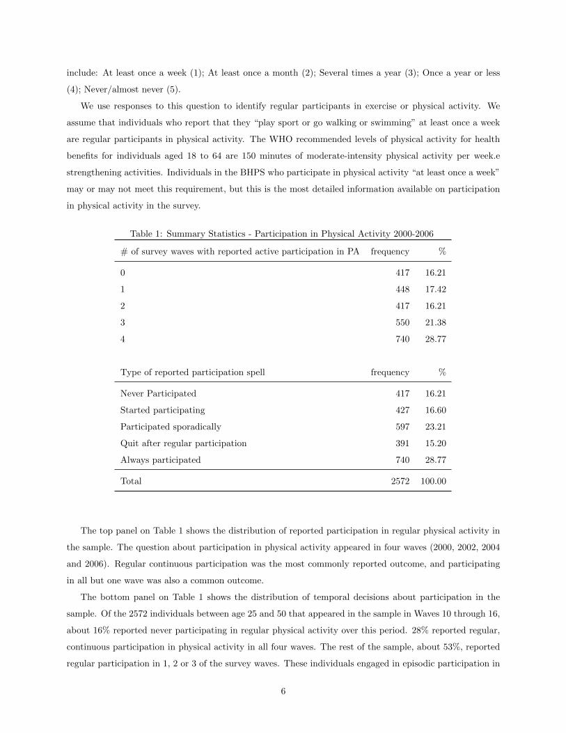
Table 1: Summary Statistics - Participation in Physical Activity 2000-2006

# of survey waves with reported active participation in PA frequency %

0 417 16.21

1 448 17.42

2 417 16.21

3 550 21.38

4 740 28.77

Type of reported participation spell frequency %

Never Participated 417 16.21

Started participating 427 16.60

Participated sporadically 597 23.21

Quit after regular participation 391 15.20

Always participated 740 28.77

Total 2572 100.00

The top panel on Table 1 shows the distribution of reported participation in regular physical activity in

the sample. The question about participation in physical activity appeared in four waves (2000, 2002, 2004

and 2006). Regular continuous participation was the most commonly reported outcome, and participating

in all but one wave was also a common outcome.

The bottom panel on Table 1 shows the distribution of temporal decisions about participation in the

sample. Of the 2572 individuals between age 25 and 50 that appeared in the sample in Waves 10 through 16,

about 16% reported never participating in regular physical activity over this period. 28% reported regular,

continuous participation in physical activity in all four waves. The rest of the sample, about 53%, reported

regular participation in 1, 2 or 3 of the survey waves. These individuals engaged in episodic participation in

6

physical activity. From the bottom panel of Table 1, about 17% were inactive at the beginning of the period

but started regular participation at a later point, and about 15% were physically active at the beginning of

the sample period and quit at some point.

These temporal patterns in participation paint a more complex picture of participation decisions than

can be seen in cross-sectional data. A substantial number of people participate regularly over a sustained

period of time, and another large group of people either quit or start regular participation over this period.

Observed participants in physical activity in cross sectional data could be regular participants or could have

recently started regular participation. Observed non-participants might never have participated or might

have recently quit after a spell of regular participation. Since the WHO recommendations stress sustained

participation, theoretical and empirical evidence that takes into account the temporal nature of participation

in physical activity can shed new light on this decision that may help to design effective interventions to

attract new participants and promote habituation to regular physical activity.

3 A model of physical activity participation decisions

We develop a behavioral economic model featuring formation, time inconsistent preferences, including naive

and sophisticated individuals, and projection bias with respect to habit formation and decay to explain

why individuals start, quit, and continue to participate in physical activity. The model also includes a

participation-specific cost shock and emphasizes the traditional economic factors that affect the decision to

participate in physical activity. The model developed here differs from DellaVigna and Malmendier (2006)

and Acland and Levy (2013) in that it applies to general decisions about leisure time participation in physical

activity, including activities like taking a walk, going for a jog or run, or performing exercises in the home.

We do not address the decision to join a gym or fitness club, and the related contracting decision involving

interaction between gym operators and potential members.4

3.1 Habit formation, Present bias, and Naivete

Consider a dynamic discrete-time, discrete choice model with periods t = 1, . . . , T . In each period individuals

either participate in physical activity (at = 1) or do not participate (at = 0). Individuals choose only current

participation and cannot commit to any future actions.

We adopt the general habit formation framework proposed by Becker and Murphy (1988) where in-

stantaneous utility in period t is ut(at, kt) and kt summarizes the history of the activity of interest. Like

O’Donoghue and Rabin (1999a) and Acland and Levy (2013), we simplify kt to be a binary state variable

where kt = at−1 = 0, 1.4DellaVigna and Malmendier (2006) develop a model of contract choice and health club attendance that includes stochastic

effort costs and delayed health benefits. Acland and Levy (2013) develop a model of gym attendance that includes habit

formation, projection bias, and present-biased preferences.

7

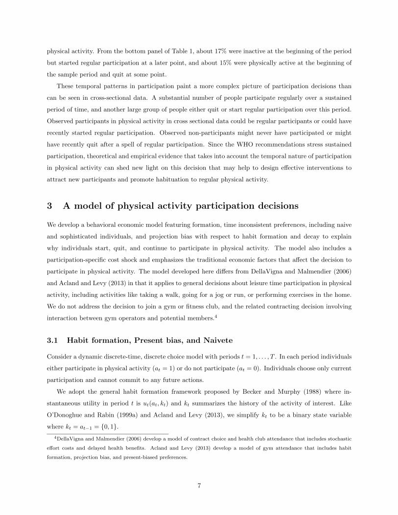
Assume that participation in physical activity involves immediate psychological, physical, time and fi-

nancial costs. et reflects immediate psychological and physical effort costs, Tt time costs, and ct the financial

costs associated with participation in physical activity. We assume that habitual physical activity reduces

psychological and physical effort costs, but not other costs, in that

et =

e if at−1 = 0

e− eh if at−1 = 1

where e > 0 and eh > 0. Note that e− eh can be positive or negative, so individuals habituated to physical

activity may experience a net immediate utility gain.5

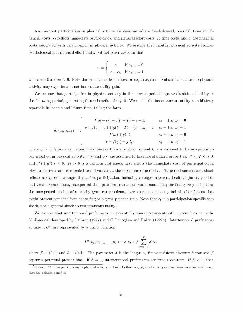
We assume that participation in physical activity in the current period improves health and utility in

the following period, generating future benefits of v > 0. We model the instantaneous utility as additively

separable in income and leisure time, taking the form

ut (at, at−1) =

f(yt − ct) + g(lt − T )− e− εt at = 1, at−1 = 0

v + f(yt − ct) + g(lt − T )− (e− eh)− εt at = 1, at−1 = 1

f(yt) + g(lt) at = 0, at−1 = 0

v + f(yt) + g(lt) at = 0, at−1 = 1

where yt and lt are income and total leisure time available. yt and lt are assumed to be exogenous to

participation in physical activity. f(·) and g(·) are assumed to have the standard properties: f ′(·), g′(·) > 0,

and f ′′(·), g′′(·) ≤ 0. εt > 0 is a random cost shock that affects the immediate cost of participation in

physical activity and is revealed to individuals at the beginning of period t. The period-specific cost shock

reflects unexpected changes that affect participation, including changes in general health, injuries, good or

bad weather conditions, unexpected time pressures related to work, commuting, or family responsibilities,

the unexpected closing of a nearby gym, car problems, over-sleeping, and a myriad of other factors that

might prevent someone from exercising at a given point in time. Note that εt is a participation-specific cost

shock, not a general shock to instantaneous utility.

We assume that intertemporal preferences are potentially time-inconsistent with present bias as in the

(β, δ)-model developed by Laibson (1997) and O’Donoghue and Rabin (1999b). Intertemporal preferences

at time t, U t, are represented by a utility function

U t(ut, ut+1, . . . , uT ) ≡ δtut + β

T∑τ=t+1

δτuτ

where β ∈ (0, 1] and δ ∈ (0, 1]. The parameter δ is the long-run, time-consistent discount factor and β

captures potential present bias. If β = 1, intertemporal preferences are time consistent. If β < 1, then

5If e−eh < 0, then participating in physical activity is “fun”. In this case, physical activity can be viewed as an entertainment

that has delayed benefits.

8

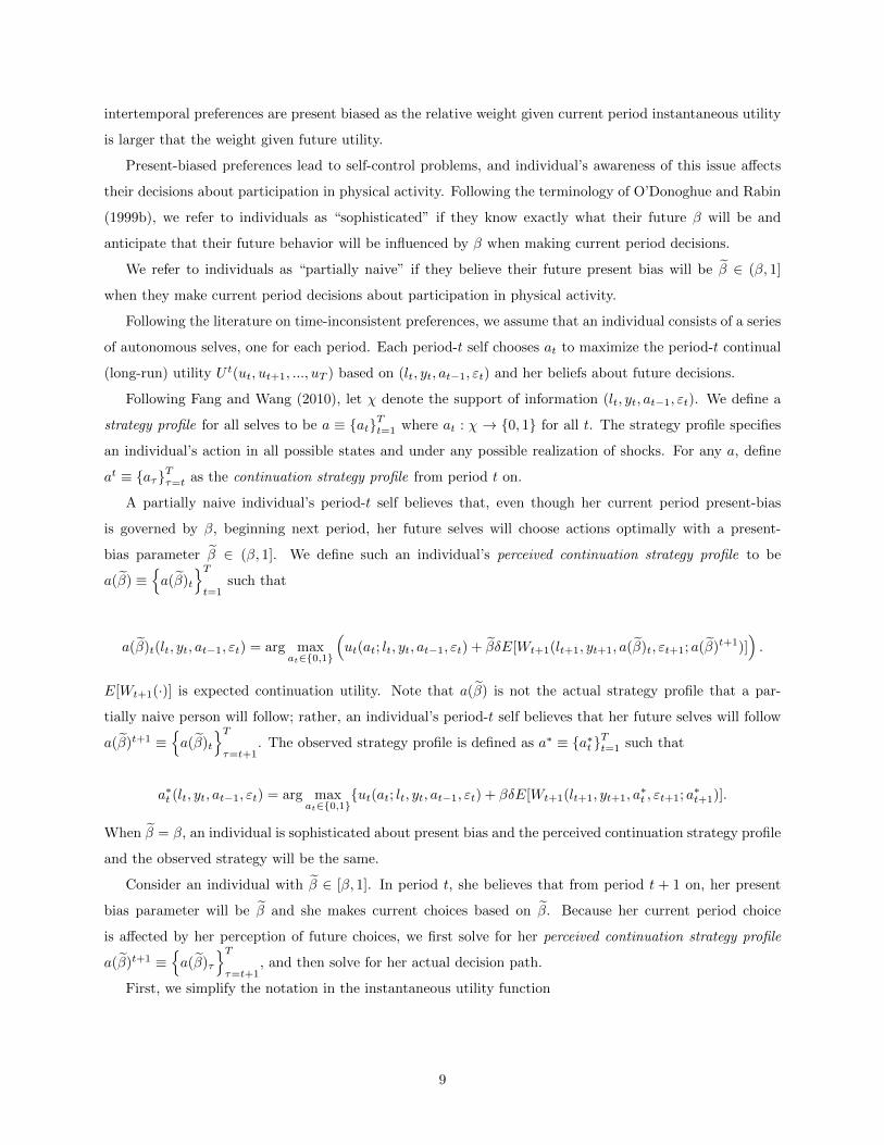
intertemporal preferences are present biased as the relative weight given current period instantaneous utility

is larger that the weight given future utility.

Present-biased preferences lead to self-control problems, and individual’s awareness of this issue affects

their decisions about participation in physical activity. Following the terminology of O’Donoghue and Rabin

(1999b), we refer to individuals as “sophisticated” if they know exactly what their future β will be and

anticipate that their future behavior will be influenced by β when making current period decisions.

We refer to individuals as “partially naive” if they believe their future present bias will be β ∈ (β, 1]

when they make current period decisions about participation in physical activity.

Following the literature on time-inconsistent preferences, we assume that an individual consists of a series

of autonomous selves, one for each period. Each period-t self chooses at to maximize the period-t continual

(long-run) utility U t(ut, ut+1, ..., uT ) based on (lt, yt, at−1, εt) and her beliefs about future decisions.

Following Fang and Wang (2010), let χ denote the support of information (lt, yt, at−1, εt). We define a

strategy profile for all selves to be a ≡ atTt=1 where at : χ → 0, 1 for all t. The strategy profile specifies

an individual’s action in all possible states and under any possible realization of shocks. For any a, define

at ≡ aτTτ=t as the continuation strategy profile from period t on.

A partially naive individual’s period-t self believes that, even though her current period present-bias

is governed by β, beginning next period, her future selves will choose actions optimally with a present-

bias parameter β ∈ (β, 1]. We define such an individual’s perceived continuation strategy profile to be

a(β) ≡a(β)t

Tt=1

such that

a(β)t(lt, yt, at−1, εt) = arg maxat∈0,1

(ut(at; lt, yt, at−1, εt) + βδE[Wt+1(lt+1, yt+1, a(β)t, εt+1; a(β)t+1)]

).

E[Wt+1(·)] is expected continuation utility. Note that a(β) is not the actual strategy profile that a par-

tially naive person will follow; rather, an individual’s period-t self believes that her future selves will follow

a(β)t+1 ≡a(β)t

Tτ=t+1

. The observed strategy profile is defined as a∗ ≡ a∗t Tt=1 such that

a∗t (lt, yt, at−1, εt) = arg maxat∈0,1

ut(at; lt, yt, at−1, εt) + βδE[Wt+1(lt+1, yt+1, a∗t , εt+1; a∗t+1)].

When β = β, an individual is sophisticated about present bias and the perceived continuation strategy profile

and the observed strategy will be the same.

Consider an individual with β ∈ [β, 1]. In period t, she believes that from period t + 1 on, her present

bias parameter will be β and she makes current choices based on β. Because her current period choice

is affected by her perception of future choices, we first solve for her perceived continuation strategy profile

a(β)t+1 ≡a(β)τ

Tτ=t+1

, and then solve for her actual decision path.

First, we simplify the notation in the instantaneous utility function

9

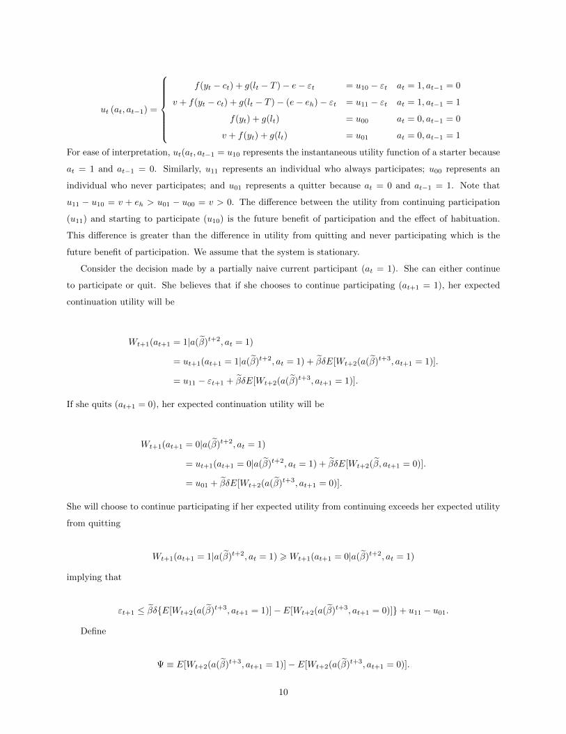
ut (at, at−1) =

f(yt − ct) + g(lt − T )− e− εt = u10 − εt at = 1, at−1 = 0

v + f(yt − ct) + g(lt − T )− (e− eh)− εt = u11 − εt at = 1, at−1 = 1

f(yt) + g(lt) = u00 at = 0, at−1 = 0

v + f(yt) + g(lt) = u01 at = 0, at−1 = 1

For ease of interpretation, ut(at, at−1 = u10 represents the instantaneous utility function of a starter because

at = 1 and at−1 = 0. Similarly, u11 represents an individual who always participates; u00 represents an

individual who never participates; and u01 represents a quitter because at = 0 and at−1 = 1. Note that

u11 − u10 = v + eh > u01 − u00 = v > 0. The difference between the utility from continuing participation

(u11) and starting to participate (u10) is the future benefit of participation and the effect of habituation.

This difference is greater than the difference in utility from quitting and never participating which is the

future benefit of participation. We assume that the system is stationary.

Consider the decision made by a partially naive current participant (at = 1). She can either continue

to participate or quit. She believes that if she chooses to continue participating (at+1 = 1), her expected

continuation utility will be

Wt+1(at+1 = 1|a(β)t+2, at = 1)

= ut+1(at+1 = 1|a(β)t+2, at = 1) + βδE[Wt+2(a(β)t+3, at+1 = 1)].

= u11 − εt+1 + βδE[Wt+2(a(β)t+3, at+1 = 1)].

If she quits (at+1 = 0), her expected continuation utility will be

Wt+1(at+1 = 0|a(β)t+2, at = 1)

= ut+1(at+1 = 0|a(β)t+2, at = 1) + βδE[Wt+2(β, at+1 = 0)].

= u01 + βδE[Wt+2(a(β)t+3, at+1 = 0)].

She will choose to continue participating if her expected utility from continuing exceeds her expected utility

from quitting

Wt+1(at+1 = 1|a(β)t+2, at = 1) >Wt+1(at+1 = 0|a(β)t+2, at = 1)

implying that

εt+1 ≤ βδE[Wt+2(a(β)t+3, at+1 = 1)]− E[Wt+2(a(β)t+3, at+1 = 0)]+ u11 − u01.

Define

Ψ ≡ E[Wt+2(a(β)t+3, at+1 = 1)]− E[Wt+2(a(β)t+3, at+1 = 0)].

10

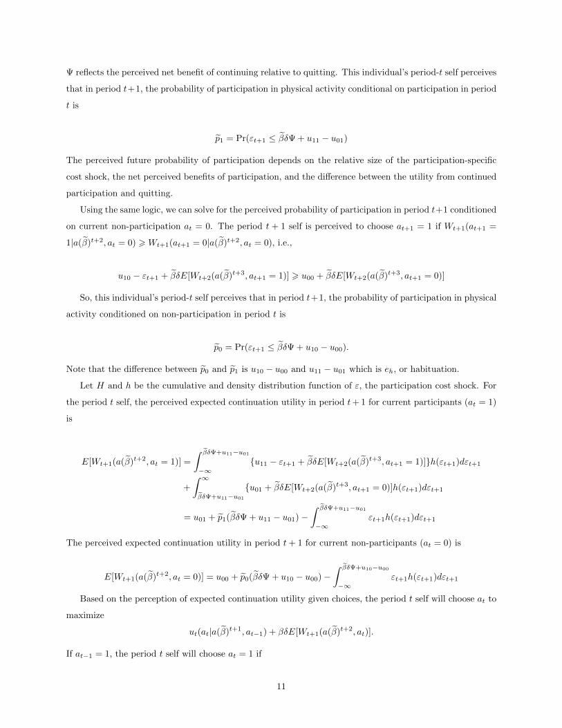
Ψ reflects the perceived net benefit of continuing relative to quitting. This individual’s period-t self perceives

that in period t+1, the probability of participation in physical activity conditional on participation in period

t is

p1 = Pr(εt+1 ≤ βδΨ + u11 − u01)

The perceived future probability of participation depends on the relative size of the participation-specific

cost shock, the net perceived benefits of participation, and the difference between the utility from continued

participation and quitting.

Using the same logic, we can solve for the perceived probability of participation in period t+1 conditioned

on current non-participation at = 0. The period t + 1 self is perceived to choose at+1 = 1 if Wt+1(at+1 =

1|a(β)t+2, at = 0) >Wt+1(at+1 = 0|a(β)t+2, at = 0), i.e.,

u10 − εt+1 + βδE[Wt+2(a(β)t+3, at+1 = 1)] > u00 + βδE[Wt+2(a(β)t+3, at+1 = 0)]

So, this individual’s period-t self perceives that in period t+1, the probability of participation in physical

activity conditioned on non-participation in period t is

p0 = Pr(εt+1 ≤ βδΨ + u10 − u00).

Note that the difference between p0 and p1 is u10 − u00 and u11 − u01 which is eh, or habituation.

Let H and h be the cumulative and density distribution function of ε, the participation cost shock. For

the period t self, the perceived expected continuation utility in period t+ 1 for current participants (at = 1)

is

E[Wt+1(a(β)t+2, at = 1)] =

∫ βδΨ+u11−u01

−∞u11 − εt+1 + βδE[Wt+2(a(β)t+3, at+1 = 1)]h(εt+1)dεt+1

+

∫ ∞βδΨ+u11−u01

u01 + βδE[Wt+2(a(β)t+3, at+1 = 0)]h(εt+1)dεt+1

= u01 + p1(βδΨ + u11 − u01)−∫ βδΨ+u11−u01

−∞εt+1h(εt+1)dεt+1

The perceived expected continuation utility in period t+ 1 for current non-participants (at = 0) is

E[Wt+1(a(β)t+2, at = 0)] = u00 + p0(βδΨ + u10 − u00)−∫ βδΨ+u10−u00


Based on the perception of expected continuation utility given choices, the period t self will choose at to

maximize

ut(at|a(β)t+1, at−1) + βδE[Wt+1(a(β)t+2, at)].

If at−1 = 1, the period t self will choose at = 1 if

11

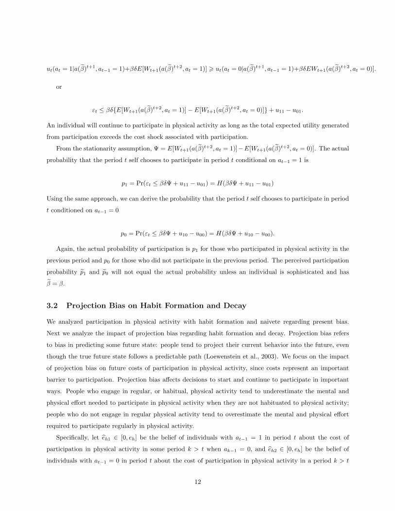
ut(at = 1|a(β)t+1, at−1 = 1)+βδE[Wt+1(a(β)t+2, at = 1)] > ut(at = 0|a(β)t+1, at−1 = 1)+βδEWt+1(a(β)t+2, at = 0)].

or

εt ≤ βδE[Wt+1(a(β)t+2, at = 1)]− E[Wt+1(a(β)t+2, at = 0)]+ u11 − u01.

An individual will continue to participate in physical activity as long as the total expected utility generated

from participation exceeds the cost shock associated with participation.

From the stationarity assumption, Ψ = E[Wt+1(a(β)t+2, at = 1)]−E[Wt+1(a(β)t+2, at = 0)]. The actual

probability that the period t self chooses to participate in period t conditional on at−1 = 1 is

p1 = Pr(εt ≤ βδΨ + u11 − u01) = H(βδΨ + u11 − u01)

Using the same approach, we can derive the probability that the period t self chooses to participate in period

t conditioned on at−1 = 0

p0 = Pr(εt ≤ βδΨ + u10 − u00) = H(βδΨ + u10 − u00).

Again, the actual probability of participation is p1 for those who participated in physical activity in the

previous period and p0 for those who did not participate in the previous period. The perceived participation

probability p1 and p0 will not equal the actual probability unless an individual is sophisticated and has

β = β.

3.2 Projection Bias on Habit Formation and Decay

We analyzed participation in physical activity with habit formation and naivete regarding present bias.

Next we analyze the impact of projection bias regarding habit formation and decay. Projection bias refers

to bias in predicting some future state: people tend to project their current behavior into the future, even

though the true future state follows a predictable path (Loewenstein et al., 2003). We focus on the impact

of projection bias on future costs of participation in physical activity, since costs represent an important

barrier to participation. Projection bias affects decisions to start and continue to participate in important

ways. People who engage in regular, or habitual, physical activity tend to underestimate the mental and

physical effort needed to participate in physical activity when they are not habituated to physical activity;

people who do not engage in regular physical activity tend to overestimate the mental and physical effort

required to participate regularly in physical activity.

Specifically, let eh1 ∈ [0, eh] be the belief of individuals with at−1 = 1 in period t about the cost of

participation in physical activity in some period k > t when ak−1 = 0, and eh2 ∈ [0, eh] be the belief of

individuals with at−1 = 0 in period t about the cost of participation in physical activity in a period k > t

12

when ak−1 = 1. We allow the projection bias to be asymmetric. In the following analysis, we assume for

simplicity that individuals are sophisticated about their present bias.

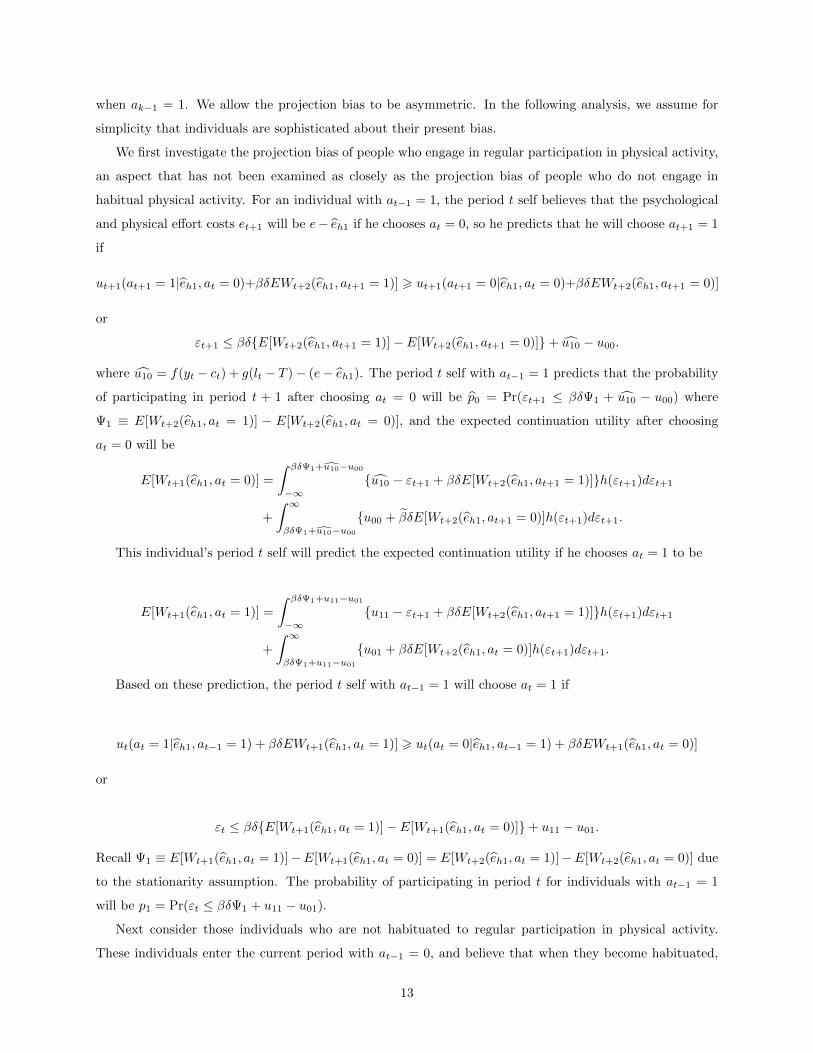
We first investigate the projection bias of people who engage in regular participation in physical activity,

an aspect that has not been examined as closely as the projection bias of people who do not engage in

habitual physical activity. For an individual with at−1 = 1, the period t self believes that the psychological

and physical effort costs et+1 will be e− eh1 if he chooses at = 0, so he predicts that he will choose at+1 = 1

if

ut+1(at+1 = 1|eh1, at = 0)+βδEWt+2(eh1, at+1 = 1)] > ut+1(at+1 = 0|eh1, at = 0)+βδEWt+2(eh1, at+1 = 0)]

or

εt+1 ≤ βδE[Wt+2(eh1, at+1 = 1)]− E[Wt+2(eh1, at+1 = 0)]+ u10 − u00.

where u10 = f(yt − ct) + g(lt − T )− (e− eh1). The period t self with at−1 = 1 predicts that the probability

of participating in period t + 1 after choosing at = 0 will be p0 = Pr(εt+1 ≤ βδΨ1 + u10 − u00) where

Ψ1 ≡ E[Wt+2(eh1, at = 1)] − E[Wt+2(eh1, at = 0)], and the expected continuation utility after choosing

at = 0 will be

E[Wt+1(eh1, at = 0)] =

∫ βδΨ1+u10−u00

−∞u10 − εt+1 + βδE[Wt+2(eh1, at+1 = 1)]h(εt+1)dεt+1

+

∫ ∞βδΨ1+u10−u00

u00 + βδE[Wt+2(eh1, at+1 = 0)]h(εt+1)dεt+1.

This individual’s period t self will predict the expected continuation utility if he chooses at = 1 to be

E[Wt+1(eh1, at = 1)] =

∫ βδΨ1+u11−u01


+

∫ ∞βδΨ1+u11−u01

u01 + βδE[Wt+2(eh1, at = 0)]h(εt+1)dεt+1.

Based on these prediction, the period t self with at−1 = 1 will choose at = 1 if

ut(at = 1|eh1, at−1 = 1) + βδEWt+1(eh1, at = 1)] > ut(at = 0|eh1, at−1 = 1) + βδEWt+1(eh1, at = 0)]

or

εt ≤ βδE[Wt+1(eh1, at = 1)]− E[Wt+1(eh1, at = 0)]+ u11 − u01.

Recall Ψ1 ≡ E[Wt+1(eh1, at = 1)]−E[Wt+1(eh1, at = 0)] = E[Wt+2(eh1, at = 1)]−E[Wt+2(eh1, at = 0)] due

to the stationarity assumption. The probability of participating in period t for individuals with at−1 = 1

will be p1 = Pr(εt ≤ βδΨ1 + u11 − u01).

Next consider those individuals who are not habituated to regular participation in physical activity.

These individuals enter the current period with at−1 = 0, and believe that when they become habituated,

13

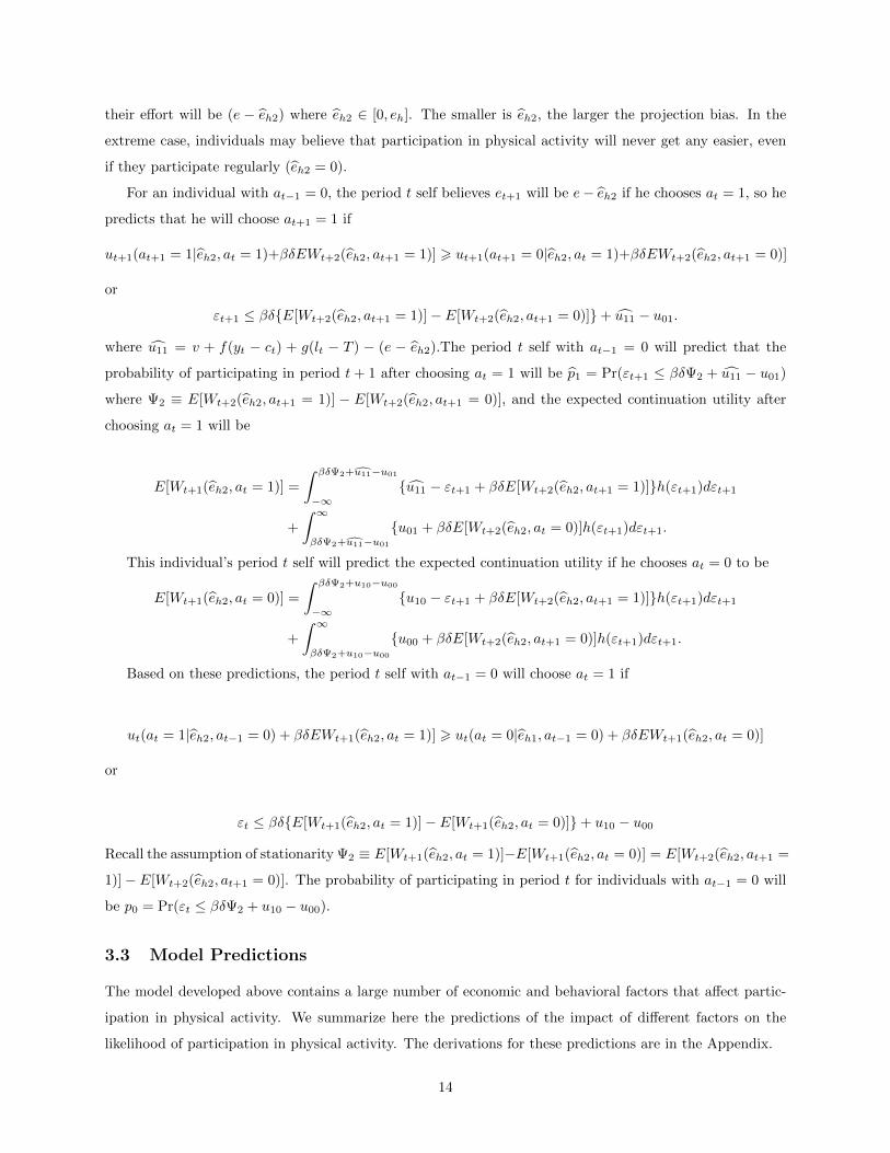
their effort will be (e − eh2) where eh2 ∈ [0, eh]. The smaller is eh2, the larger the projection bias. In the

extreme case, individuals may believe that participation in physical activity will never get any easier, even

if they participate regularly (eh2 = 0).

For an individual with at−1 = 0, the period t self believes et+1 will be e− eh2 if he chooses at = 1, so he

predicts that he will choose at+1 = 1 if

ut+1(at+1 = 1|eh2, at = 1)+βδEWt+2(eh2, at+1 = 1)] > ut+1(at+1 = 0|eh2, at = 1)+βδEWt+2(eh2, at+1 = 0)]

or

εt+1 ≤ βδE[Wt+2(eh2, at+1 = 1)]− E[Wt+2(eh2, at+1 = 0)]+ u11 − u01.

where u11 = v + f(yt − ct) + g(lt − T ) − (e − eh2).The period t self with at−1 = 0 will predict that the

probability of participating in period t + 1 after choosing at = 1 will be p1 = Pr(εt+1 ≤ βδΨ2 + u11 − u01)

where Ψ2 ≡ E[Wt+2(eh2, at+1 = 1)] − E[Wt+2(eh2, at+1 = 0)], and the expected continuation utility after

choosing at = 1 will be

E[Wt+1(eh2, at = 1)] =

∫ βδΨ2+u11−u01


+

∫ ∞βδΨ2+u11−u01

u01 + βδE[Wt+2(eh2, at = 0)]h(εt+1)dεt+1.

This individual’s period t self will predict the expected continuation utility if he chooses at = 0 to be

E[Wt+1(eh2, at = 0)] =

∫ βδΨ2+u10−u00


+

∫ ∞βδΨ2+u10−u00

u00 + βδE[Wt+2(eh2, at+1 = 0)]h(εt+1)dεt+1.

Based on these predictions, the period t self with at−1 = 0 will choose at = 1 if

ut(at = 1|eh2, at−1 = 0) + βδEWt+1(eh2, at = 1)] > ut(at = 0|eh1, at−1 = 0) + βδEWt+1(eh2, at = 0)]

or

εt ≤ βδE[Wt+1(eh2, at = 1)]− E[Wt+1(eh2, at = 0)]+ u10 − u00

Recall the assumption of stationarity Ψ2 ≡ E[Wt+1(eh2, at = 1)]−E[Wt+1(eh2, at = 0)] = E[Wt+2(eh2, at+1 =

1)]− E[Wt+2(eh2, at+1 = 0)]. The probability of participating in period t for individuals with at−1 = 0 will

be p0 = Pr(εt ≤ βδΨ2 + u10 − u00).

3.3 Model Predictions

The model developed above contains a large number of economic and behavioral factors that affect partic-

ipation in physical activity. We summarize here the predictions of the impact of different factors on the

likelihood of participation in physical activity. The derivations for these predictions are in the Appendix.

14

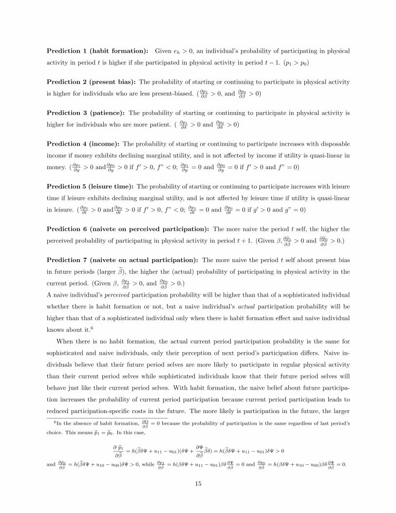
Prediction 1 (habit formation): Given eh > 0, an individual’s probability of participating in physical

activity in period t is higher if she participated in physical activity in period t− 1. (p1 > p0)

Prediction 2 (present bias): The probability of starting or continuing to participate in physical activity

is higher for individuals who are less present-biased. (∂p1

∂β > 0, and ∂p0

∂β > 0)

Prediction 3 (patience): The probability of starting or continuing to participate in physical activity is

higher for individuals who are more patient. ( ∂p1

∂δ > 0 and ∂p0

∂δ > 0)

Prediction 4 (income): The probability of starting or continuing to participate increases with disposable

income if money exhibits declining marginal utility, and is not affected by income if utility is quasi-linear in

money. (∂p1

∂y > 0 and∂p0

∂y > 0 if f ′ > 0, f” < 0; ∂p1

∂y = 0 and ∂p0

∂y = 0 if f ′ > 0 and f” = 0)

Prediction 5 (leisure time): The probability of starting or continuing to participate increases with leisure

time if leisure exhibits declining marginal utility, and is not affected by leisure time if utility is quasi-linear

in leisure. (∂p1

∂l > 0 and∂p0

∂l > 0 if f ′ > 0, f” < 0; ∂p1

∂l = 0 and ∂p0

∂l = 0 if g′ > 0 and g” = 0)

Prediction 6 (naivete on perceived participation): The more naive the period t self, the higher the

perceived probability of participating in physical activity in period t+ 1. (Given β,∂p1

∂β> 0 and ∂p0

∂β> 0.)

Prediction 7 (naivete on actual participation): The more naive the period t self about present bias

in future periods (larger β), the higher the (actual) probability of participating in physical activity in the

current period. (Given β, ∂p1

∂β> 0, and ∂p0

∂β> 0.)

A naive individual’s perceived participation probability will be higher than that of a sophisticated individual

whether there is habit formation or not, but a naive individual’s actual participation probability will be

higher than that of a sophisticated individual only when there is habit formation effect and naive individual

knows about it.6

When there is no habit formation, the actual current period participation probability is the same for

sophisticated and naive individuals, only their perception of next period’s participation differs. Naive in-

dividuals believe that their future period selves are more likely to participate in regular physical activity

than their current period selves while sophisticated individuals know that their future period selves will

behave just like their current period selves. With habit formation, the naive belief about future participa-

tion increases the probability of current period participation because current period participation leads to

reduced participation-specific costs in the future. The more likely is participation in the future, the larger

6In the absence of habit formation, ∂Ω

∂β= 0 because the probability of participation is the same regardless of last period’s

choice. This means p1 = p0. In this case,

∂ p1

∂β= h(βδΨ + u11 − u01)(δΨ +

∂Ψ

∂ββδ) = h(βδΨ + u11 − u01)δΨ > 0

and ∂p0

∂β= h(βδΨ + u10 − u00)δΨ > 0, while ∂p1

∂β= h(βδΨ + u11 − u01)βδ ∂Ψ

∂β= 0 and ∂p0

∂β= h(βδΨ + u10 − u00)βδ ∂Ψ

∂β= 0.

15

the benefit from current period participation. This is a case where naivety about present bias leads to a

higher probability of a preferred choice by the long-run self.

How could sophistication lead to worse outcomes than naivete? Remember, in the model we rule out

the possibility of any commitment devices. If individuals are allowed to use commitment devices, then

sophisticated individuals, knowing their self-control problems, will be more likely to pre-commit their future

selves to achieve the outcome their long-run selves would prefer. Naive individuals do not seek commitment

devices because they are not aware of their future self-control problem.

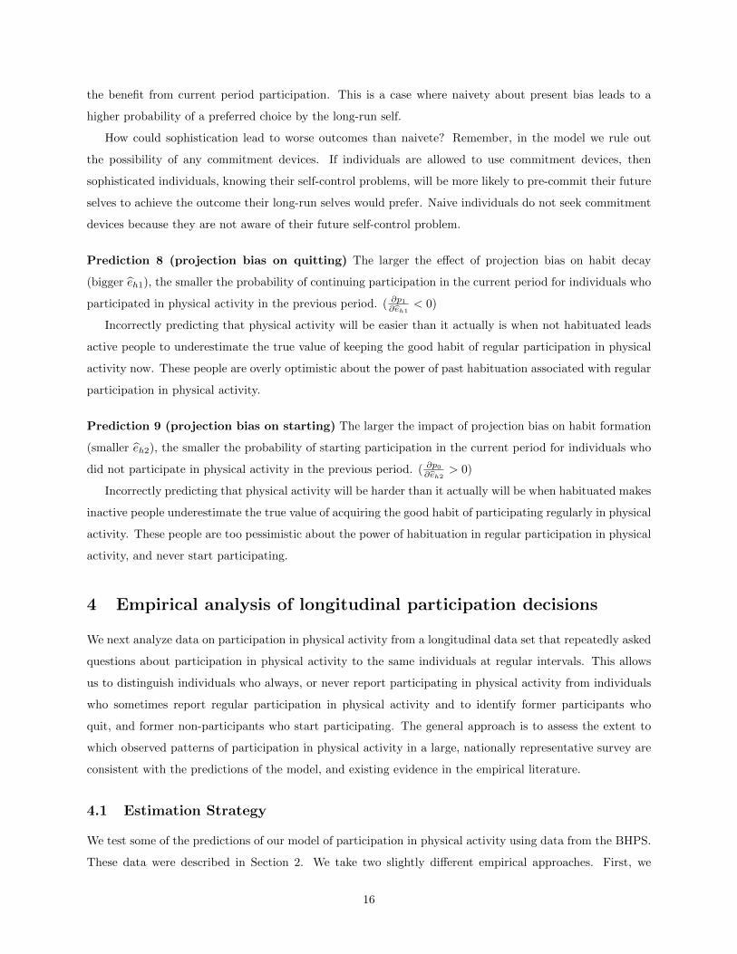
Prediction 8 (projection bias on quitting) The larger the effect of projection bias on habit decay

(bigger eh1), the smaller the probability of continuing participation in the current period for individuals who

participated in physical activity in the previous period. ( ∂p1

∂eh1< 0)

Incorrectly predicting that physical activity will be easier than it actually is when not habituated leads

active people to underestimate the true value of keeping the good habit of regular participation in physical

activity now. These people are overly optimistic about the power of past habituation associated with regular


Prediction 9 (projection bias on starting) The larger the impact of projection bias on habit formation

(smaller eh2), the smaller the probability of starting participation in the current period for individuals who

did not participate in physical activity in the previous period. ( ∂p0

∂eh2> 0)

Incorrectly predicting that physical activity will be harder than it actually will be when habituated makes

inactive people underestimate the true value of acquiring the good habit of participating regularly in physical

activity. These people are too pessimistic about the power of habituation in regular participation in physical

activity, and never start participating.

4 Empirical analysis of longitudinal participation decisions

We next analyze data on participation in physical activity from a longitudinal data set that repeatedly asked

questions about participation in physical activity to the same individuals at regular intervals. This allows

us to distinguish individuals who always, or never report participating in physical activity from individuals

who sometimes report regular participation in physical activity and to identify former participants who

quit, and former non-participants who start participating. The general approach is to assess the extent to

which observed patterns of participation in physical activity in a large, nationally representative survey are

consistent with the predictions of the model, and existing evidence in the empirical literature.

4.1 Estimation Strategy

We test some of the predictions of our model of participation in physical activity using data from the BHPS.

These data were described in Section 2. We take two slightly different empirical approaches. First, we

16

analyze the decision to quit participating after engaging in regular participation (the QUIT model) and

the decision to start participating after being physically inactive (the START model). As suggested by the

theoretical model, habit formation (and decay) and potential projection bias create an asymmetry between

quitting and starting.7 Second, we explore the history of past participation on current participation to test

the habit formation and decay effect.

4.1.1 Models of Starting and Quitting

We estimate separate probit models for starting or quitting regular participation in physical activity. In one

case, the QUIT model, the dependent variable yi is equal to one if individual i reported quitting regular

participation in physical activity later in the sample after earlier reporting regular participation. In the

other case, the START model, the dependent variable yi equal to one if individual i reported starting

regular participation in physical activity later in the sample after reporting inactivity earlier in the sample.

yi is equal to zero for individuals who reported continued regular participation in the QUIT model and for

those who reported continued inactivity in the START model.

The probit models estimated take the form

yi = f(γ,Xi, εi) (1)

where Xi is a vector of covariates, γ a vector of unobserved parameters to be estimated, and εi an unobserv-

able error term that captures other factors that affect individual’s decisions about participation in physical

activity. We assume that εi is distributed with mean zero and constant variance. f(·) is the cumulative

distribution function of the standard normal distribution. We estimate γ using maximum likelihood and

transform the estimates of γ into marginal effects that show the change in the conditional probability that

yi = 1 associated with a one unit change in each covariate. The vector of explanatory variables Xi contains

the variables reflecting the demographic and economics conditions faced by each respondent that might affect

the decision to participate in physical activity and proxy variables for present bias and other psychological

conditions.

Many factors may explain participation in physical activity, some may be unobservable to econometri-

cians. In order to control for unobservable heterogeneity, we restrict our sample to individuals appearing in

the BHPS in all seven waves administered between 2000 and 2006. We also restrict the sample to individuals

who were at least 25 years of age in 2000, and less than 50 years of age in 2006. This helps to control for

the effects of school attendance and retirement decisions on the decision to participate in physical activity.

We extract a number of variables related to education, employment, income, and other factors from the

BHPS that are frequently included in empirical models of participation in physical activity. Table 2 contains

7Grignon (2009) also find present bias has different impact on starting and quitting smoking. Quitting smoking is hard

because smoking brings instant gratification and delayed health benefits. Similarly, stating participation is hard because it

involves current costs and delayed health benefits.

17

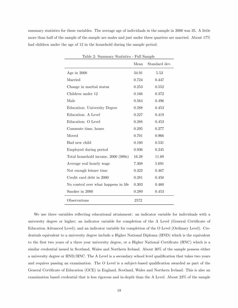
summary statistics for these variables. The average age of individuals in the sample in 2000 was 35. A little

more than half of the sample of the sample are males and just under three quarters are married. About 17%

had children under the age of 12 in the household during the sample period.

Table 2: Summary Statistics - Full Sample

Mean Standard dev.

Age in 2000 34.91 5.53

Married 0.724 0.447

Change in marital status 0.253 0.552

Children under 12 0.166 0.372

Male 0.564 0.496

Education: University Degree 0.288 0.453

Education: A Level 0.227 0.419

Education: O Level 0.288 0.453

Commute time, hours 0.295 0.277

Moved 0.701 0.966

Had new child 0.160 0.531

Employed during period 0.936 0.245

Total household income, 2000 (000s) 16.28 11.69

Average real hourly wage 7.308 5.691

Not enough leisure time 0.322 0.467

Credit card debt in 2000 0.281 0.450

No control over what happens in life 0.303 0.460

Smoker in 2000 0.289 0.453

Observations 2572

We use three variables reflecting educational attainment: an indicator variable for individuals with a

university degree or higher; an indicator variable for completion of the A Level (General Certificate of

Education Advanced Level); and an indicator variable for completion of the O Level (Ordinary Level). Cre-

dentials equivalent to a university degree include a Higher National Diploma (HND) which is the equivalent

to the first two years of a three year university degree, or a Higher National Certificate (HNC) which is a

similar credential issued in Scotland, Wales and Northern Ireland. About 30% of the sample possess either

a university degree or HND/HNC. The A Level is a secondary school level qualification that takes two years

and requires passing an examination. The O Level is a subject-based qualification awarded as part of the

General Certificate of Education (GCE) in England, Scotland, Wales and Northern Ireland. This is also an

examination based credential that is less rigorous and in-depth than the A Level. About 23% of the sample

18

passed the A Level exams and 29% passed the O level. The omitted educational attainment category is

individuals without a university degree, A Level or O level; these individuals make up about 20% of the

sample.

During the study period, 94% of the sample was employed at some point. From Table 2, the average time

commuting to work for individuals in the sample was about 30 minutes. The BHPS also asks respondents to

assess the amount time available for leisure activities. A feeling that there is not enough leisure time serves

as a general proxy for the presence of time constraints. 32% of the sample reported feeling they did not have

enough leisure time. Total household income in 2000 was 16,279 pounds sterling.

The variables moved, had new child, and change in marital status reflect events that are disruptive, at

least temporarily, to one’s daily schedule and raise participation costs to some extent. Not all these events

are unexpected, but the size of the effect of, say, a new child in the household, may be difficult to assess

before the event occurs. A rather large percentage of the sample (70%) moved during the study period. A

quarter of the sample had a change in marital status and 16% had a new child during the sample period.

A final group of control variables are proxies for present bias. The first proxy variable is an indicator

variable for individuals who reported positive credit card debt 2000. Credit card debt has been found to

be associated with present bias (Meier and Sprenger, 2010). The second proxy variable is an indicator for

reported smoking in 2000. Smoking has been linked to present biased time preferences in previous research

(Burks et al. (2012), Grignon (2009) and Kang and Ikeda (2013)). About 28-29% of the sample exhibit these

behaviors.

We also include an indicator variable for individuals with weak locus of control. The BPHS contains a

question that assesses the extent to which respondents feel they have control of their life, in other words a

self-assessed locus of control proxy: “I feel that what happens to me is out of my control.” We construct an

indicator variable that is equal to one if an individual responded either “sometimes” or “often” when asked

the frequency with which they have this feeling and zero otherwise.

4.1.2 History of Past Participation

Charness and Gneezy (2009) and Acland and Levy (2015) find evidence supporting the importance of habit

formation in health club exercise. These studies randomly assign individuals into groups that receive or do

not receive financial incentives to exercise in health clubs and track their attendance over time. They find a

significant post-intervention attendance increase of the treated groups relative to the control groups.

The model developed above assumes that past participation reduces effort costs of current participation

and predicts that past participation in physical activity increases the probability of current participation

(Prediction 1). We lack access to a “natural experiment” that would randomly increase the benefit to exercise

for some survey respondents in these data; but we observe participation decisions for each individual over

a sufficiently long period of time. This allows us to undertake simple tests of the effect of habit formation

19

on current participation decisions, assuming past participation is partly driven by the realization of the

stochastic period-specific participation cost shock.

These tests analyze decisions about participation in regular physical activity in 2006 when controlling

for past participation decisions and other individual characteristics. First, we estimate Probit models of the

general form

pi,2006 = α0 +

3∑j=1

αjpi,2006−2j + γXi + εi (2)

where pi,t is an indicator variable that is equal to one if individual i participated regularly in physical activity

in BHPS survey wave t and zero otherwise. pi,t reflects each individual’s history of participation in regular

physical activity throughout the sample period. Xi is a vector of individual economic and demographic

characteristics measured in 2000, or in some cases over the 2000-2006 period. εi is an unobserved random

error term capturing all other factors that affect the participation decision. The αs and γ are unobservable

parameters to be estimated.

Alternative to the habit formation and decay hypothesis, an empirical correlation between past participa-

tion and current participation can purely because of unobserved personal traits. If there is no effect of habit

formation and decay and past participation is correlated with current participation through time-invariant

unobservable personal traits, then the coefficient on the three past participation variables should be the same.

So, the personal traits hypothesis implies α1 = α2 = α3 while the habit formation and decay hypothesis

implies α1 > α2 > α3.

Another hypothesis relates to learning through participation. If there is no habit formation but people

generally over-estimate the true effort costs of participation, then actual participation in one period can lead

them to learn about actual effort costs, increasing the probability of future participation. To investigate this

alternative hypothesis, we break our sample into two subsamples. The first subsample includes individuals

who reported regular participation in physical activity in both 2000 and 2002 (pi,2000 = 1 and pi,2002 =

1). This subsample contains 1,061 individuals. The second subsample includes individuals who did not

report regular participation in physical activity in either 2000 or 2002 (pi,2000 = 0 and pi,2002 = 0). This

subsample contains 760 individuals. The individuals in the first subsample had a relatively long history of past

participation while the individuals in the second subsample had a relatively long history of non-participation.

We argue that learning learning should not be very important for individuals in the first subsample because

they participated in the recent past. However, learning might have an effect for individuals in the second

subsample because these individuals have not been physically active for quite some time, and they may

incorrectly predict the effort needed to participate in physical activity. We estimate Probit models

pi,2006 = α0 + α1pi,2004 + γXi + εi. (3)

The learning hypothesis implies α1 = 0 for the regression with the first subsample and α1 > 0 for the

regression with the second subsample, while habit formation and decay implies α1 > 0 for both subsamples.

20

4.2 Results

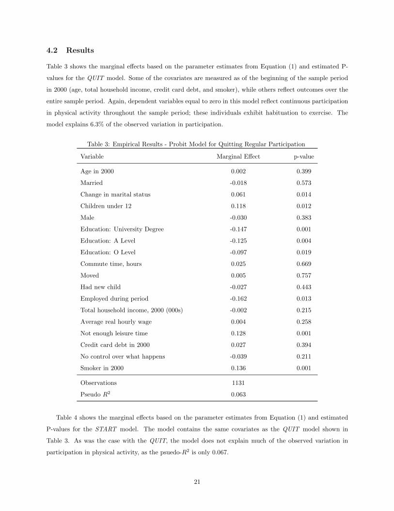
Table 3 shows the marginal effects based on the parameter estimates from Equation (1) and estimated P-

values for the QUIT model. Some of the covariates are measured as of the beginning of the sample period

in 2000 (age, total household income, credit card debt, and smoker), while others reflect outcomes over the

entire sample period. Again, dependent variables equal to zero in this model reflect continuous participation

in physical activity throughout the sample period; these individuals exhibit habituation to exercise. The

model explains 6.3% of the observed variation in participation.

Table 3: Empirical Results - Probit Model for Quitting Regular Participation

Variable Marginal Effect p-value

Age in 2000 0.002 0.399

Married -0.018 0.573



Male -0.030 0.383

Education: University Degree -0.147 0.001

Education: A Level -0.125 0.004

Education: O Level -0.097 0.019

Commute time, hours 0.025 0.669

Moved 0.005 0.757

Had new child -0.027 0.443

Employed during period -0.162 0.013

Total household income, 2000 (000s) -0.002 0.215


Not enough leisure time 0.128 0.001

Credit card debt in 2000 0.027 0.394

No control over what happens -0.039 0.211

Smoker in 2000 0.136 0.001

Observations 1131

Pseudo R2 0.063

Table 4 shows the marginal effects based on the parameter estimates from Equation (1) and estimated

P-values for the START model. The model contains the same covariates as the QUIT model shown in

Table 3. As was the case with the QUIT, the model does not explain much of the observed variation in

participation in physical activity, as the psuedo-R2 is only 0.067.

21

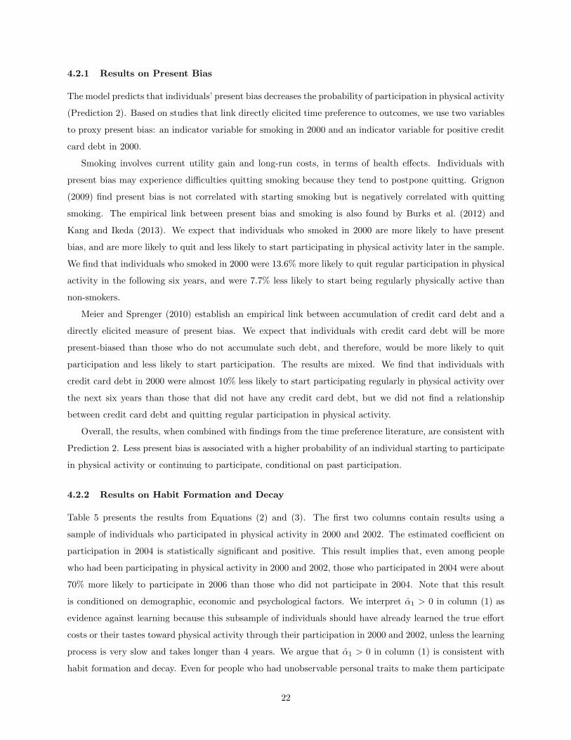
4.2.1 Results on Present Bias

The model predicts that individuals’ present bias decreases the probability of participation in physical activity

(Prediction 2). Based on studies that link directly elicited time preference to outcomes, we use two variables

to proxy present bias: an indicator variable for smoking in 2000 and an indicator variable for positive credit

card debt in 2000.

Smoking involves current utility gain and long-run costs, in terms of health effects. Individuals with

present bias may experience difficulties quitting smoking because they tend to postpone quitting. Grignon

(2009) find present bias is not correlated with starting smoking but is negatively correlated with quitting

smoking. The empirical link between present bias and smoking is also found by Burks et al. (2012) and

Kang and Ikeda (2013). We expect that individuals who smoked in 2000 are more likely to have present

bias, and are more likely to quit and less likely to start participating in physical activity later in the sample.

We find that individuals who smoked in 2000 were 13.6% more likely to quit regular participation in physical

activity in the following six years, and were 7.7% less likely to start being regularly physically active than

non-smokers.

Meier and Sprenger (2010) establish an empirical link between accumulation of credit card debt and a

directly elicited measure of present bias. We expect that individuals with credit card debt will be more

present-biased than those who do not accumulate such debt, and therefore, would be more likely to quit

participation and less likely to start participation. The results are mixed. We find that individuals with

credit card debt in 2000 were almost 10% less likely to start participating regularly in physical activity over

the next six years than those that did not have any credit card debt, but we did not find a relationship

between credit card debt and quitting regular participation in physical activity.

Overall, the results, when combined with findings from the time preference literature, are consistent with

Prediction 2. Less present bias is associated with a higher probability of an individual starting to participate

in physical activity or continuing to participate, conditional on past participation.

4.2.2 Results on Habit Formation and Decay

Table 5 presents the results from Equations (2) and (3). The first two columns contain results using a

sample of individuals who participated in physical activity in 2000 and 2002. The estimated coefficient on

participation in 2004 is statistically significant and positive. This result implies that, even among people

who had been participating in physical activity in 2000 and 2002, those who participated in 2004 were about

70% more likely to participate in 2006 than those who did not participate in 2004. Note that this result

is conditioned on demographic, economic and psychological factors. We interpret α1 > 0 in column (1) as

evidence against learning because this subsample of individuals should have already learned the true effort

costs or their tastes toward physical activity through their participation in 2000 and 2002, unless the learning

process is very slow and takes longer than 4 years. We argue that α1 > 0 in column (1) is consistent with

habit formation and decay. Even for people who had unobservable personal traits to make them participate

22

Table 4: Empirical Results - Probit Model for Starting Regular Participation

Variable Marginal Effect p-value

Age in 2000 -0.013 0.001

Married -0.017 0.668



Male -0.027 0.512

Education: University Degree 0.114 0.026

Education: A Level -0.021 0.663

Education: O Level -0.045 0.311

Commute time, hours -0.140 0.047

Moved 0.032 0.072

Had new child 0.010 0.775

Employed during period 0.060 0.370

Total household income, 2000 (000s) -0.001 0.930


Not enough leisure time -0.045 0.172

Credit card debt in 2000 -0.096 0.007

No control over what happens -0.084 0.017

Smoker in 2000 -0.077 0.025

Observations 902

Pseudo R2 0.070

23

in 2000 and 2002, had acquired the habit of regular participation, and potentially had learned the nature of

physical activity, stopping in 2004 significantly reduces their probability of participating in 2006, suggesting

that participating in physical activity is a rather delicate habit that decays quickly and requires careful

maintenance.

Columns 3 and 4 in Table 5 show the results using the sample of individuals who did not participate in

physical activity in 2000 or 2002. The estimated coefficient on participation in 2004 is statistically significant

and positive. This result implies that, among people who did not participate in physical activity in 2000 or

2002, those who participated in 2004 were about 76% more likely to participate in 2006 than those who did

not participate in 2004. We interpret α1 > 0 in column (1) to be consistent with a combination of learning

and habit formation. We do not know whether these individuals had participated before 2000 but it is safe

to say that they had a relatively long recent history of non-participation right before 2004. Participating in

2004 may help them learn or form a habit, both of which could increase their probability of participating

in 2006. The result suggests that encouraging people who have been inactive for a long time in the past

to participate now may have a temporal externality through habit formation and learning. Compared to

α1 > 0 in column (1), the size of the point estimate in column (2) is only slightly bigger, suggesting that the

effect of learning might be small compared to the effect of habit formation.

Columns and 6 in Table 5 contain results using the entire sample of prime age individuals who appeared

in every wave of the BHPS from 2000 to 2006. The estimated coefficient on the indicator variable for

participation in 2004 (α1), participation in 2002 (α2), and participation in 2000 (α3) are all positive and

significantly different from zero. Suppose the unobservable personal traits that make people more or less

likely to participate in physical activity is time invariant, then the pure personal traits hypothesis implies

α1 = α2 = α3. The result (α1 > α2 > α3) argues against the pure personal traits hypothesis. Note that it

does not rule out the effect of time-invariant personal traits, but personal traits alone cannot fully explain the

temporal correlation in participation. The result shows that more recent participation has a larger impact

on current participation (α1 > α2 > α3) and is consistent with the presence of habit formation and habit

decay.

Overall, the results in Table 5 suggest learning and time invariant personal traits cannot fully explain

the temporal pattern of participation in physical activity. The results are consistent with the hypothesis

that participation in physical activity is a habit that is subject to significant decay if not maintained. The

results are also consistent with positive serial correlation in the cost shocks associated with participation.

4.2.3 Other Socioeconomic and Psychological Factors

We now discuss the role of other demographic and psychological factors and compare the results in Table

3 to findings from cross-sectional studies. Studying physical activity behavior over time has the potential

to provide some important insight to the episodic nature of physical activity that cannot be gleaned from

cross-sectional or repeated cross-sectional data.

24

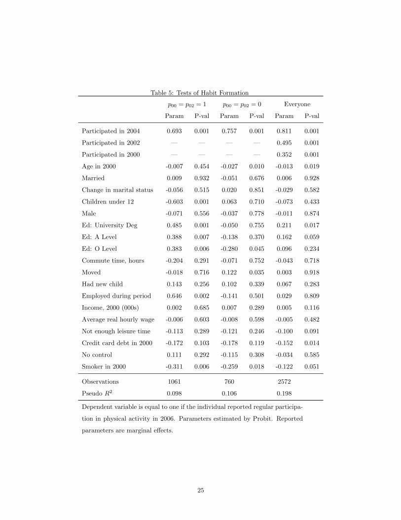
Table 5: Tests of Habit Formation

p00 = p02 = 1 p00 = p02 = 0 Everyone

Param P-val Param P-val Param P-val

Participated in 2004 0.693 0.001 0.757 0.001 0.811 0.001

Participated in 2002 — — — — 0.495 0.001

Participated in 2000 — — — — 0.352 0.001

Age in 2000 -0.007 0.454 -0.027 0.010 -0.013 0.019

Married 0.009 0.932 -0.051 0.676 0.006 0.928

Change in marital status -0.056 0.515 0.020 0.851 -0.029 0.582

Children under 12 -0.603 0.001 0.063 0.710 -0.073 0.433

Male -0.071 0.556 -0.037 0.778 -0.011 0.874

Ed: University Deg 0.485 0.001 -0.050 0.755 0.211 0.017

Ed: A Level 0.388 0.007 -0.138 0.370 0.162 0.059

Ed: O Level 0.383 0.006 -0.280 0.045 0.096 0.234

Commute time, hours -0.204 0.291 -0.071 0.752 -0.043 0.718

Moved -0.018 0.716 0.122 0.035 0.003 0.918

Had new child 0.143 0.256 0.102 0.339 0.067 0.283

Employed during period 0.646 0.002 -0.141 0.501 0.029 0.809

Income, 2000 (000s) 0.002 0.685 0.007 0.289 0.005 0.116

Average real hourly wage -0.006 0.603 -0.008 0.598 -0.005 0.482

Not enough leisure time -0.113 0.289 -0.121 0.246 -0.100 0.091

Credit card debt in 2000 -0.172 0.103 -0.178 0.119 -0.152 0.014

No control 0.111 0.292 -0.115 0.308 -0.034 0.585

Smoker in 2000 -0.311 0.006 -0.259 0.018 -0.122 0.051

Observations 1061 760 2572

Pseudo R2 0.098 0.106 0.198

Dependent variable is equal to one if the individual reported regular participa-

tion in physical activity in 2006. Parameters estimated by Probit. Reported

parameters are marginal effects.

25

The probability that an individual quits participation in physical activity at some point in the sample

after previously reporting regular participation is not associated with age in this sample as the marginal

effect, while positive and small, is not statistically different from zero. Contrary to the results for the QUIT

model, age did have an impact on decisions to start regular participation in physical activity. In this sample,

older individuals in 2000 were 1.3% less likely to become physically active than younger individuals. The

negative relationship between age and participation in physical activity from cross-sectional studies is likely

due to reluctance to start rather than inclination to quit participation when people get older. This finding

is important because the policy implication regarding the timing of policy intervention might be different.

Our result suggests that for a particular individual, an intervention of the same size is more likely to induce

participation when she is young.

Married individuals were no less likely to report quitting participation than singles, and males no less

likely than females. The marginal effects for married and male were not statistically significant in the START

model just as they were not significant in the QUIT model. These findings differ from the results of most, if

not all, cross-sectional studies of physical activity. Most studies find that men are more likely to participate

than women, and that married people are less likely to participate than single individuals.

Education has an important impact on the probability of quitting participation in physical activity.

All individuals with a university degree, A level or O level credential were less likely to report quitting

participation in physical activity and that the probability of quitting increases with less education. Those

with a university degree were 14.5% less likely to quit participation in physical activity, compared to 12.2%

for those with A level and 9.4% for those with O level. In contrast with the QUIT model, education is

not a particularly important factor influencing decisions to start participating in physical activity. The only

education variable that is significant is university degree. Respondents with a university degree were 10%

more likely to start participating in physical activity than those without a higher education credential.

Another variable commonly included in studies about participation in physical activity is the presence of

children in the household. Results from cross-sectional studies are mixed with respect to the presence of chil-

dren. Some studies find that the presence of very young children is negatively associated with participation

but that the presence of “older” children in the household is positively associated with participation. The

exact specification of this variable is driven by data, but most surveys ask questions reflecting the presence

of children under the age of 12, as is the case with the BHPS, or very young children, usually under the

age of 5. Our results indicate that the presence of children under the age of 12 was associated with a 12%

greater probability of quitting regular participation but was not correlated with the probability of starting

regularly participating in physical activity. Taken together the results from the QUIT and the START

model, having young children appears to exert an overall negative pressure on physical activity participation

in that an individual might quit when there are young children in the house, but this individual who quit

due to young children in the house is not more likely to participate when there are no young children in the

26

house (e.g., children grow up). This result reinforces the importance of habit formation and decay in regular


Our findings regarding the role of labor market conditions and income differ somewhat from those of many

studies using cross-sectional studies where income generally is positively related to participation and being

employed is negatively related to participation. Most of the variables measuring labor market conditions,

employed during period, total household income,8 and average real hourly wage were not significantly different

from zero, except employed during period in the QUIT model. Individuals who were employed during the

sample period were 15.7% less likely to quit engaging in physical activity. We also include commuting time

and wages in our regressions. The coefficient of wages was not significantly different from zero in either the

QUIT or the START model indicating no relationship to the probability of quitting or starting participation.

Individuals with a longer commute to work were less likely to start participating in physical activity but

commuting time was not significantly correlated with quitting. Very few studies have measures of wages and

even fewer, if any, include commuting time.

Next we investigate the role of major events that are likely to change people’s lives, including moving, a

change in marital status, and having a new child. Moving was not significant in the QUIT model but has a

positive effect on the decision to start participating. A change in marital status was associated with a 6.4%

increase in the probability of quitting but was not correlated with the probability of starting. Having a new

child was not statistically significant in either the QUIT or START models.

We also find some interesting asymmetric impacts on quitting and starting with respect to the time

constraint and internal locus of control. Individuals who felt they do not have enough leisure time were

12.8% more likely to quit engaging in physical activity than those who felt they had enough leisure time,

but not having enough leisure time was not associated with the decision to start participation. Individuals

who felt like they had no control over what happens in life, those with weak internal locus of control, were

8.4% less likely to start regularly participating in physical activity, but weak internal locus of control was

not associated with the decision to quit participation.

5 Conclusions

A substantial number of individuals decided to start regular participation in common forms of sport and

exercise like walking and swimming, or quit regular participation in these activities, over the six year period

analyzed here. Documenting the frequency of starts, quits, and episodic participation in physical activity is

important to further our understanding of this important health behavior. Most current evidence uses survey

data collected at a single point in time, or repeated cross-sectional survey data over time, to develop evidence

about factors associated with participation in physical activity. This evidence compares current participants

to current non-participants. Since the surveys typically ask questions about participation in the last few

8The same result was obtained when this variable was replaced with labor income and investment income.

27

weeks or months, little can be learned about the temporal nature of participation in physical activity.9

Individuals who report not participating in physical activity in a cross sectional survey that asks about

participation in the last month or six months could be individuals who never participate, or alternatively

they could be episodic participants who happen to be in a period of non-participation. Our empirical analysis

discover some interesting dynamic patterns in quitting and starting participating in physical activity that

cross sectional data will not be able to reveal.

Previous research established the importance of present bias, habit formation, naivete and projection bias

in gym contract choice and attendance decisions (Acland and Levy (2015), Charness and Gneezy (2009),

DellaVigna and Malmendier (2006), and Garon et al. (2013)). We develop a dynamic discrete-time, discrete

choice model incorporating these important behavioral factors and abstracting from the contracting aspects

associated with health club membership and attendance. Our model helps to understand the dynamic de-

cision to participate in general leisure time physical activity, which may not involve a complicated contract

choice. The model generates a rich set of predicts regarding these behavioral factors and traditional economic

factors. We find empirical results consistent with predictions regarding present-bias and habit formation us-

ing the BHPS, a nationally representative longitudinal sample. Predictions regarding naivete and projection

bias are not directly testable with our data, but the theoretical implication suggests that these are important

areas for future empirical investigation that may benefit policy making.

Many public policy initiatives focus on encouraging individuals to take up healthy habits like regular

participation in physical activity. These programs often approach the lack of participation in physical activ-

ity as the result of lack of information, and provide information about the benefits of regular participation

in physical activity. Implicitly, these campaigns assume that after learning about the future benefits of

regular participation, inactive individuals will revise their forecasts and some may choose to start partici-

pating regularly. These campaigns ignore the possibility that self-control problems due to present bias, and

misperception of the effect of habit formation and decay in participating in physical activity may act as

barriers to starting regular participation. In addition, these campaigns are not targeted towards people who

are currently active, implicitly assuming they will stay active. If self-control problems negatively affect both

inactive and active individuals, then educating people about their present bias and the importance of devel-

oping commitment tools should be important. If participating in physical activity is a habit but decays, then

it is important not only to educate inactive people about the habit formation effect to encourage starting,

but also to educate active people about the habit decay effect to discourage quitting.

We acknowledge that our results must be understood in the context of the existing literature and our

identification assumptions. Our data do not have directly elicited time preference measures or a clean

“natural experiment” for habit formation. We draw from studies using directly elicited time preference

measures and behavioral outcomes (Burks et al. (2012), Grignon (2009), Kang and Ikeda (2013), and Meier

9Cavaco et al. (2014) develop evidence of episodic participation in exercise at ages 25, 35, 45, and at their current age, using

retrospective data collected through an internet survey conducted in six European countries.

28

and Sprenger (2010)), and use smoking and the accumulation of credit card debt to proxy for present bias.

Our test of the habit formation (and decay) hypothesis against the pure personal traits hypothesis and the

learning hypothesis explores the history of past participation and assumes away positive serial correlation in

unobservable participation shocks. We believe that the theoretical model and empirical analysis can inspire

additional empirical investigation to reach more definitive conclusions about the role of behavioral factors in

the dynamic decision to participate in physical activity for general populations.

References

Acland, D. and Levy, M. (2013). Habit formation, naivete, and projection bias in gym attendance. Working

paper.

Acland, D. and Levy, M. R. (2015). Naivete, projection bias, and habit formation in gym attendance.

Management Science, 61(1):146–160.

Anokye, N. K., Pokhrel, S., Buxton, M., and Fox-Rushby, J. (2012). The demand for sports and exercise:

results from an illustrative survey. The European Journal of Health Economics, 13(3):277–287.

Becker, G. S. and Murphy, K. M. (1988). A theory of rational addiction. The Journal of Political Economy,

96(4):675–700.

Brown, H. and Roberts, J. (2011). Exercising choice: The economic determinants of physical activity

behaviour of an employed population. Social Science & Medicine, 73(3):383–390.

Burks, S., Carpenter, J., Gotte, L., and Rustichini, A. (2012). Which measures of time preference best predict

outcomes: Evidence from a large-scale field experiment. Journal of Economic Behavior & Organization,

84(1):308–320.

Cavaco, S., Eriksson, T., and Skalli, A. (2014). Life cycle development of obesity and its determinants in six

European countries. Economics & Human Biology, 14:62–78.

Charness, G. and Gneezy, U. (2009). Incentives to exercise. Econometrica, 77(3):909–931.

Cobb-Clark, D. A., Kassenboehmer, S. C., and Schurer, S. (2014). Healthy habits: The connection between

diet, exercise, and locus of control. Journal of Economic Behavior & Organization, 98:1–28.

DellaVigna, S. and Malmendier, U. (2006). Paying Not to Go to the Gym. American Economic Review,

96(3):694–719.

Downward, P. (2007). Exploring the economic choice to participate in sport: Results from the 2002 General

Household Survey. International Review of Applied Economics, 21(5):633–653.

29

Eisenberg, D. and Okeke, E. (2009). Too cold for a jog? weather, exercise, and socioeconomic status. The

BE Journal of Economic Analysis & Policy, 9(1).

Fang, H. and Wang, Y. (2010). Estimating dynamic discrete choice models with hyperbolic discounting, with

an application to mammography decisions. Technical report, National Bureau of Economic Research.

Farrell, L. and Shields, M. A. (2002). Investigating the economic and demographic determinants of sporting

participation in England. Journal of the Royal Statistical Society (Series B), 165(2):335–348.

Fildes, A., Charlton, J., Rudisill, C., Littlejohns, P., Prevost, A. T., and Gulliford, M. C. (2015). Probability

of an obese person attaining normal body weight: Cohort study using electronic health records. American

Journal of Public Health, 105(9):e54–e59.

Garcıa, J., Lera-Lopez, F., and Suarez, M. J. (2011). Estimation of a structural model of the determinants of

the time spent on physical activity and sport evidence for spain. Journal of Sports Economics, 12(5):515–

537.

Garon, J.-D., Masse, A., and Michaud, P.-C. (2013). Health club attendance, expectations and self-control.

Technical Report 13-17, CIRPEE. Cahier de recherche/Working Paper.

Grignon, M. (2009). An empirical investigation of heterogeneity in time preferences and smoking behaviors.

The Journal of Socio-Economics, 38(5):739–751.

Humphreys, B. R., McLeod, L., and Ruseski, J. E. (2014). Physical activity and health outcomes: evidence

from Canada. Health Economics, 23(1):33–54.

Humphreys, B. R. and Ruseski, J. E. (2007). Participation in physical activity and government spending on

parks and recreation. Contemporary Economic Policy, 25(4):538–552.

Humphreys, B. R. and Ruseski, J. E. (2011). An economic analysis of participation and time spent in

physical activity. The BE Journal of Economic Analysis & Policy, 11(1):1–38.

Kang, M.-I. and Ikeda, S. (2013). Time discounting and smoking behavior: Evidence from a panel survey.

Health Economics, 23(12):1443–1464.

Kokolakakis, T., Lera-Lopez, F., and Panagouleas, T. (2012). Analysis of the determinants of sports partic-

ipation in Spain and England. Applied Economics, 44(21):2785–2798.

Laibson, D. (1997). Golden eggs and hyperbolic discounting. The Quarterly Journal of Economics,

112(2):443–477.

Loewenstein, G., O’Donoghue, T., and Rabin, M. (2003). Projection bias in predicting future utility. The

Quarterly Journal of Economics, 118(4):pp. 1209–1248.

30

Meier, S. and Sprenger, C. (2010). Present-biased preferences and credit card borrowing. American Economic

Journal: Applied Economics, 2(1):193–210.

O’Donoghue, T. and Rabin, M. (1999a). Addiction and self-control. Addiction: Entries and exits, pages

169–206.

O’Donoghue, T. and Rabin, M. (1999b). Doing it now or later. American Economic Review, 89(1):103–124.

World Health Organization (2010). Global Recommendations on Physical Activity for Health. WHO Report,

World Health Organization.

31

Appendix

Derivation of Predictions

1. Habit formation

p1 − p0 = H(βδΨ + u11 − u01)−H(βδΨ + u10 − u00)

= H(βδΨ + u10 − u00 + eh)−H(βδΨ + u10 − u00) > 0.

∂p1

∂δ = h(βδΨ + u11 − u01)(βΨ + ∂Ψ∂δ ) > 0

∂p0

∂δ = h(βδΨ + u10 − u00)(βΨ + ∂Ψ∂δ ) > 0

∂p1

∂β = h(βδΨ + u11 − u01)(δΨ + βδ ∂Ψ∂β ) > 0

∂p0

∂β = h(βδΨ + u10 − u00)(δΨ + βδ ∂Ψ∂β ) > 0

2. Present Bias: See text.

3. Patience: See text.

4. Income

∂p1

∂y= h(βδΨ + u11 − u01)[βδ

∂Ψ

∂y+∂(u11 − u01)

∂y]

and

∂Ψ

∂y= −

∂Ω∂y

∂Ω∂Ψ

= 0

and

∂(u11 − u01)

∂y= 0

if f(y) = kyy. Also, if f ′ > 0, f” < 0, then ∂(u11−u01)∂y = ∂(u10−u00)

∂y = f ′(y − c)− f ′(y) > 0, and

∂Ω

∂y= −βδ(∂p1

∂y− ∂p0

∂y)Ψ− ∂p1

∂y(u11 − u01) +

∂p0

∂y(u10 − u00) +

∫ βδΨ+u11−u01

−∞ εt+1h(εt+1)dεt+1

∂y

−∫ βδΨ+u10−u00


∂y− p1

∂(u11 − u01)

∂y+ p0

∂(u10 − u00)

∂y

= (p0 − p1)[f ′(y − c)− f ′(y)] < 0

Therefore, ∂Ψ∂y = −

∂Ω∂y∂Ω∂Ψ

> 0 and ∂p1

∂y > 0. Using the same method ∂p0

∂y = h(βδΨ + u10 − u00)[βδ ∂Ψ∂y +

∂(u10−u00)∂y ] > 0 if f ′ > 0, f” < 0, and ∂p0

∂y = 0 if f ′ > 0 and f” = 0.

5. Leisure time

The derivation of this prediction is omitted as it follows the same procedure as the derivation of the

income effect.

32

6./7. Naivete

From above, p1 = Pr(εt+1 ≤ βδΨ + u11 − u01). It follows that

∂p1

∂β= h(βδΨ + u11 − u01)(δΨ +

∂Ψ

∂ββδ).

Since naivety increases the probability future participation, the perceived net benefit of continuing partici-

pation is positive, Ψ = E[Wt+1(a(β)t+2, at = 1)] − E[Wt+1(a(β)t+2, at = 0)] > 0, because at = 1 generates

more utility than at = 0 regardless of at+1.

Next, we show that ∂Ψ

∂β> 0. Partial naivety increases the perceived net benefit of future participation.

From the stationarity assumption

Ψ = E[Wt+1(a(β)t+2, at = 1)]− E[Wt+1(a(β)t+2, at = 0)]

= u01 − u00 + βδ(p1 − p0)Ψ + p1(u11 − u01)− p0(u10 − u00)

−∫ βδΨ+u11−u01

−∞εt+1h(εt+1)dεt+1 +

∫ βδΨ+u10−u00


Rearranging this equation

[1− βδ(p1 − p0)]Ψ− p1(u11 − u01) + p0(u10 − u00) +

∫ βδΨ+u11−u01


−∫ βδΨ+u10−u00

−∞εt+1h(εt+1)dεt+1 = u01 − u00 = v

Define the left side of the above equation as Ω. Differentiating Ω with respect to Ψ

∂Ω

∂Ψ= [1− βδ(p1 − p0)]− βδ(∂p1

∂Ψ− ∂p0

∂Ψ)Ψ− ∂p1

∂Ψ(u11 − u01) +

∂p0

∂Ψ(u10 − u00)

+

∫ βδΨ+u11−u01


∂Ψ−∫ βδΨ+u10−u00


∂Ψ

= [1− βδ(p1 − p0)]− βδh(βδΨ + u11 − u01)(βδΨ + u11 − u01) + βδh(βδΨ + u10 − u00)(βδΨ + u11 − u01)

+ βδh(βδΨ + u11 − u01)(βδΨ + u11 − u01)− βδh(βδΨ + u10 − u00)(βδΨ + u11 − u01)

= 1− βδ(p1 − p0) > 0

Differentiating Ω with respect to β

33

∂Ω

∂β= −δ(p1 − p0)]Ψ− βδ(∂p1

∂β− ∂p0

∂β)Ψ− ∂p1

∂β(u11 − u01) +

∂p0

∂β(u10 − u00)

+

∫ βδΨ+u11−u01


∂β−∫ βδΨ+u10−u00


∂β

= −δ(p1 − p0)]Ψ−

∂p1

∂β(βδΨ + u11 − u01)−

∫ βδΨ+u11−u01


∂β

+

∂p0

∂β(βδΨ + u10 − u00)−

∫ βδΨ+u10−u00


∂β

= −δ(p1 − p0)]Ψ < 0

Using the implicit function theorem

∂Ψ

∂β= −

∂Ω

∂β

∂Ω∂Ψ

> 0.

Therefore,

∂ p1

∂β= h(βδΨ + u11 − u01)(δΨ +

∂Ψ

∂ββδ) > 0

and

∂ p0

∂β= h(βδΨ + u10 − u00)(δΨ +

∂Ψ

∂ββδ) > 0.

Naivety also affects actual current participation in physical activity. This follows because

∂p1

∂β= h(βδΨ + u11 − u01)βδ

∂Ψ

∂β> 0

and

∂p0

∂β= h(βδΨ + u10 − u00)βδ

∂Ψ

∂β> 0

8. Projection bias on quitting or continuing

Under the assumption of stationarity,

Ψ1 ≡ E[Wt+1(eh1, at = 1)]− E[Wt+1(eh1, at = 0)] = E[Wt+2(eh1, at+1 = 1)]− E[Wt+2(eh1, at+1 = 0)].

The stationary condition above can be rewritten

[1− βδ(p1 − p0)]Ψ1 − p1(u11 − u01) + p0(u10 − u00) +

∫ βδΨ1+u11−u01

βδΨ1+u10−u00

εt+1h(εt+1)dεt+1 = v.

34

This relationship requires additional attention, as it describes the participation decision under projection

bias. Define Ω1 as the left hand side of the above equation and take the derivative with respect to Ψ1

∂Ω1

∂Ψ1= 1− βδ(p1 − p0) > 0

To see the effect of habituation in this context, differentiate Ω1 with respect to eh1

∂Ω1

∂eh1= βδΨ1

∂p0

∂eh1+

∂p0

∂eh1(u10 − u00) + p0

∂(u10 − u00)

∂eh1− (βδΨ1 + u10 − u00)h(βδΨ1 + u10 − u00)

∂(u10 − u00)

∂eh1

= p0 > 0

Using the implicit function theorem

∂Ψ1

∂eh1= −

∂Ω1

∂eh1

∂Ω1

∂Ψ1

< 0.

Therefore, ∂p1

∂eh1= h(βδΨ1 + u11 − u01)βδ ∂Ψ1

∂eh1< 0.

9. Projection bias on starting

The stationarity assumption implies

[1− βδ(p1 − p0)]Ψ2 − p1(u11 − u01) + p0(u10 − u00) +

∫ βδΨ2+u11−u01

βδΨ2+u10−u00

εt+1h(εt+1)dεt+1 = v.

Define the left side of the above equation as Ω2 and take the derivative with respect to Ψ2

∂Ω2

∂Ψ2= 1− βδ(p1 − p0) > 0

Differentiating Ω2 with respect to eh2 gives

∂Ω2

∂eh2= −βδΨ2

∂p1

∂eh2− ∂p1

∂eh2(u11 − u01)− p1

∂(u11 − u01)

∂eh1+ (βδΨ2 + u11 − u01)h(βδΨ2 + u11 − u01)

∂(u11 − u01)

∂eh1

= −p1 < 0.

Finally, from the implicit function theorem

∂Ψ2

∂eh2= −

∂Ω2

∂eh2

∂Ω2

∂Ψ2

> 0.

From this expression, it follows that

∂p0

∂eh2= h(βδΨ2 + u10 − u00)βδ

∂Ψ2

∂eh2> 0.

35

Documents

Physical Activity, Present Bias, and Habit Formation