Physics 53

Elect!city and OpticsLaboratory Course Manual

Fall 2005

In"ructorsT. Donnelly

J. EckertD. Hoard

T. LynnG. Lyzenga

P. Saeta

Joseph von Fraunhofer Carl Friedrich Gauss Gustav Kirchhoff

name

“Nothing in the world can take the place of persistence. Talentwill not; nothing is more common than unsuccessful men withtalent. Genius will not; unrewarded genius is almost a proverb.Education will not; the world is full of educated derelicts. Per-sistence and determination alone are omnipotent.”

Calvin Coolidge

Contents

I Introductory Material iii

Quick Start Guide for First Meetings iv

Schedule v

Overview vi

General Instructions ix

Philosophical Musings xii

II Experiments 1

1 Basic DC Circuits 2

1.1 Overview . . . . . . . . . . . . . . . . . . . . . . . . . . . . . . . . . . . . . . . . . . . . . . . . . . . . 21.2 Theory . . . . . . . . . . . . . . . . . . . . . . . . . . . . . . . . . . . . . . . . . . . . . . . . . . . . . . 21.3 Precautions . . . . . . . . . . . . . . . . . . . . . . . . . . . . . . . . . . . . . . . . . . . . . . . . . . . 31.4 Procedure . . . . . . . . . . . . . . . . . . . . . . . . . . . . . . . . . . . . . . . . . . . . . . . . . . . . 4

1.4.1 Resistors in series . . . . . . . . . . . . . . . . . . . . . . . . . . . . . . . . . . . . . . . . . . . . 41.4.2 Resistors in parallel . . . . . . . . . . . . . . . . . . . . . . . . . . . . . . . . . . . . . . . . . . 41.4.3 Circuit loading . . . . . . . . . . . . . . . . . . . . . . . . . . . . . . . . . . . . . . . . . . . . . 51.4.4 Charge and discharge of a capacitor in an RC circuit (optional) . . . . . . . . . . . . . . . . . . 5

2 Absolute Current 6

2.1 Overview . . . . . . . . . . . . . . . . . . . . . . . . . . . . . . . . . . . . . . . . . . . . . . . . . . . . 62.2 Background . . . . . . . . . . . . . . . . . . . . . . . . . . . . . . . . . . . . . . . . . . . . . . . . . . . 62.3 Theory . . . . . . . . . . . . . . . . . . . . . . . . . . . . . . . . . . . . . . . . . . . . . . . . . . . . . . 82.4 Experimental Equipment and Procedures . . . . . . . . . . . . . . . . . . . . . . . . . . . . . . . . . . 10

2.4.1 Preliminary setup . . . . . . . . . . . . . . . . . . . . . . . . . . . . . . . . . . . . . . . . . . . 102.4.2 The Current coil . . . . . . . . . . . . . . . . . . . . . . . . . . . . . . . . . . . . . . . . . . . . 102.4.3 Compass deflection measurements . . . . . . . . . . . . . . . . . . . . . . . . . . . . . . . . . . 112.4.4 The Bar magnet and torsional oscillations . . . . . . . . . . . . . . . . . . . . . . . . . . . . . . 11

2.5 Experimental Analysis . . . . . . . . . . . . . . . . . . . . . . . . . . . . . . . . . . . . . . . . . . . . . 122.5.1 Fitting . . . . . . . . . . . . . . . . . . . . . . . . . . . . . . . . . . . . . . . . . . . . . . . . . . 12

3 RLC Resonance 14

3.1 Overview . . . . . . . . . . . . . . . . . . . . . . . . . . . . . . . . . . . . . . . . . . . . . . . . . . . . 143.2 Theory . . . . . . . . . . . . . . . . . . . . . . . . . . . . . . . . . . . . . . . . . . . . . . . . . . . . . . 15

3.2.1 AC voltages as complex numbers . . . . . . . . . . . . . . . . . . . . . . . . . . . . . . . . . . . 153.2.2 Complex impedance . . . . . . . . . . . . . . . . . . . . . . . . . . . . . . . . . . . . . . . . . . 16

3.3 Experimental Procedure . . . . . . . . . . . . . . . . . . . . . . . . . . . . . . . . . . . . . . . . . . . . 173.3.1 Equipment and software . . . . . . . . . . . . . . . . . . . . . . . . . . . . . . . . . . . . . . . . 17

3.4 Analyzing a circuit with more than one element . . . . . . . . . . . . . . . . . . . . . . . . . . . . . . . 203.5 Instructions for Using the Igor RLC Application . . . . . . . . . . . . . . . . . . . . . . . . . . . . . . 213.6 Program Details . . . . . . . . . . . . . . . . . . . . . . . . . . . . . . . . . . . . . . . . . . . . . . . . 24

3.6.1 Uncertainties . . . . . . . . . . . . . . . . . . . . . . . . . . . . . . . . . . . . . . . . . . . . . . 24

i

CONTENTS CONTENTS

4 Geometrical Optics 254.1 Overview . . . . . . . . . . . . . . . . . . . . . . . . . . . . . . . . . . . . . . . . . . . . . . . . . . . . 254.2 Background and Theory — Refraction . . . . . . . . . . . . . . . . . . . . . . . . . . . . . . . . . . . . 264.3 Experimental Procedures — Refraction . . . . . . . . . . . . . . . . . . . . . . . . . . . . . . . . . . . 26

4.3.1 Measurements . . . . . . . . . . . . . . . . . . . . . . . . . . . . . . . . . . . . . . . . . . . . . 274.3.2 Analysis . . . . . . . . . . . . . . . . . . . . . . . . . . . . . . . . . . . . . . . . . . . . . . . . . 27

4.4 Background and Theory — Lenses . . . . . . . . . . . . . . . . . . . . . . . . . . . . . . . . . . . . . . 284.4.1 Diverging lens . . . . . . . . . . . . . . . . . . . . . . . . . . . . . . . . . . . . . . . . . . . . . . 29

4.5 Expt. Proc. — Image Formation . . . . . . . . . . . . . . . . . . . . . . . . . . . . . . . . . . . . . . . 304.5.1 Preliminaries . . . . . . . . . . . . . . . . . . . . . . . . . . . . . . . . . . . . . . . . . . . . . . 304.5.2 Converging lens . . . . . . . . . . . . . . . . . . . . . . . . . . . . . . . . . . . . . . . . . . . . . 314.5.3 Diverging lens . . . . . . . . . . . . . . . . . . . . . . . . . . . . . . . . . . . . . . . . . . . . . . 324.5.4 Chromatic aberration . . . . . . . . . . . . . . . . . . . . . . . . . . . . . . . . . . . . . . . . . 324.5.5 Depth of field . . . . . . . . . . . . . . . . . . . . . . . . . . . . . . . . . . . . . . . . . . . . . . 32

5 Fraunhofer Diffraction 335.1 Overview . . . . . . . . . . . . . . . . . . . . . . . . . . . . . . . . . . . . . . . . . . . . . . . . . . . . 335.2 Background and Theory . . . . . . . . . . . . . . . . . . . . . . . . . . . . . . . . . . . . . . . . . . . . 33

5.2.1 Single slit . . . . . . . . . . . . . . . . . . . . . . . . . . . . . . . . . . . . . . . . . . . . . . . . 345.2.2 Double slit . . . . . . . . . . . . . . . . . . . . . . . . . . . . . . . . . . . . . . . . . . . . . . . 345.2.3 Multiple slits . . . . . . . . . . . . . . . . . . . . . . . . . . . . . . . . . . . . . . . . . . . . . . 35

5.3 Experimental Procedures . . . . . . . . . . . . . . . . . . . . . . . . . . . . . . . . . . . . . . . . . . . 355.3.1 Alignment procedure and preliminary observations . . . . . . . . . . . . . . . . . . . . . . . . . 355.3.2 Removing the photocell mount . . . . . . . . . . . . . . . . . . . . . . . . . . . . . . . . . . . . 365.3.3 Potentiometer . . . . . . . . . . . . . . . . . . . . . . . . . . . . . . . . . . . . . . . . . . . . . . 375.3.4 Beam profile . . . . . . . . . . . . . . . . . . . . . . . . . . . . . . . . . . . . . . . . . . . . . . 375.3.5 Taking data . . . . . . . . . . . . . . . . . . . . . . . . . . . . . . . . . . . . . . . . . . . . . . . 385.3.6 Program details . . . . . . . . . . . . . . . . . . . . . . . . . . . . . . . . . . . . . . . . . . . . . 395.3.7 Saved data . . . . . . . . . . . . . . . . . . . . . . . . . . . . . . . . . . . . . . . . . . . . . . . 39

6 Grating Spectrometer 416.1 Overview . . . . . . . . . . . . . . . . . . . . . . . . . . . . . . . . . . . . . . . . . . . . . . . . . . . . 416.2 Theory . . . . . . . . . . . . . . . . . . . . . . . . . . . . . . . . . . . . . . . . . . . . . . . . . . . . . . 416.3 Using the Spectrometer . . . . . . . . . . . . . . . . . . . . . . . . . . . . . . . . . . . . . . . . . . . . 43

6.3.1 Focusing procedure . . . . . . . . . . . . . . . . . . . . . . . . . . . . . . . . . . . . . . . . . . . 436.4 Experimental Measurements . . . . . . . . . . . . . . . . . . . . . . . . . . . . . . . . . . . . . . . . . . 45

6.4.1 Grating calibration . . . . . . . . . . . . . . . . . . . . . . . . . . . . . . . . . . . . . . . . . . . 456.4.2 Hydrogen observations . . . . . . . . . . . . . . . . . . . . . . . . . . . . . . . . . . . . . . . . . 466.4.3 Forensic investigation . . . . . . . . . . . . . . . . . . . . . . . . . . . . . . . . . . . . . . . . . 46

6.5 Experimental Analysis . . . . . . . . . . . . . . . . . . . . . . . . . . . . . . . . . . . . . . . . . . . . . 46

III Appendices 48

A Electric Shock – it’s the Current that Kills 49

B Resistors and Resistance Measurements 51

C Electrical Techniques and Diagrams 53

D Technical Report 54

Physics 53 Lab Manual ii August 1, 2005

Part I

Introductory Material

iii

Quick Start Guide for First Meetings

The following is a brief summary of the essential in-formation you’ll need to prepare for the first meetingsof E&M Lab. Further details will be found elsewherein this manual and in the other resources provided toyou by the instructors.

First Meeting

The first meetings of each lab section will be dur-ing the week of Aug. 29 (except for Monday sectionswhich will first meet on Sept. 5). The sections will thenmeet on succeeding weeks for two hours throughout thesemester, following the schedule of meetings and breakson the following page. Although it is not heavy, there issome preparation for the first meeting. In the first meet-ing there will be a brief orientation by the instructor toall the experiments, with related discussions of meth-ods of data analysis. You will then perform Experiment1, which is an introduction to simple DC electrical cir-cuits. Prior to coming to lab, you must read the labmanual introduction and description for Experiment1 (pp. i–xiii, 1–5). Also come to lab prepared with abrown cover National Brand #43-648 ComputationNotebook (available from the bookstore). Experiment1 is shorter and simpler than the other experiments inthe course, so you should be able to complete it in theabbreviated time available and experience a relativelyeasy “warm-up” for the later lab activities.

Plotting Exercise

In this course, everyone will be responsible for be-ing fluent in a data plotting/fitting software pack-age. To help reinforce this, everyone is required tocomplete and turn in a data plotting exercise. Assoon as possible (but before your #2a meeting) goto the web page at http://www.physics.hmc.edu/analysis/exercise.php and complete the exercise.Turn in the finished plot to your instructor.

Subsequent Meetings

After the first week, you will perform four of thefive available experiments according to a schedule to beworked out with your instructor. With your instructor’sconsultation, you will sign up for the experiments andlab partners you will work with during the semester.

The experiments in this course are challenging, and

require advance reading and preparation! It is veryimportant that you come to the lab prepared. Be-fore the first laboratory meeting for a particular ex-periment, read the appropriate section of this lab man-ual and watch the short movie introducing the exper-iment you will be doing. The movies are available atthe course web site: http://www.physics.hmc.edu/courses/p053/. We will not require pre-lab homeworkor exercises; however, part of your grade will be basedon your instructor’s assessment of how prepared you arefor lab.

The semester schedule has built-in days off from labmeetings, so please take advantage of this in managingyour time, and remember to budget time for lab prepa-ration. The lab periods run for 2 hours every meeting,and each experiment (except #1) will take two lab pe-riods. The first week (meeting “a”) will typically beuseful for familiarizing yourself with and calibrating theapparatus and making a first set of measurements; thesecond week (meeting “b”) will normally be used forcompletion of data taking, recovery from any problemsor mistakes in the first week, and consultation with yourinstructor about analysis and write-up.

Write-up of the Experiment

A typical experiment summary is 2–3 typed pages,turned in along with your lab notebook for documen-tary support, at a time and place to be announced byeach instructor. All write-ups should be typed/wordprocessed, with all graphics neatly and professionallyincorporated. An example is available on the courseweb site. The experiment summary will be what is pri-marily read and marked by your instructor. The labbook may not be graded in detail, however the degreeto which it serves as a valid reproducible archival recordof your work in lab will form a part of your grade. In thewrite-up, you may assume your reader is familiar withyour experiment, the apparatus, and the basic proce-dures, so re-hashing of these is not needed. However,you should detail innovations, important observations,or unique insights that you have made during the ex-periment period. The write-up should be entirely de-rived from the content of your laboratory notebook, andnot from memory or other undocumented sources. Seethe rest of this manual for more detailed discussion ofwriteups and lab books.

Physics 53 Lab Manual iv August 1, 2005

Schedule

Section 1 Section 3 Section 5 Section 6 Section 8 Section 10M 12:40 Tu 12:40 W 12:40 W 15:15 Th 12:40 F 12:40

Week of Donnelly Lynn Saeta Eckert Lyzenga Hoard

1 8/29 Expt. 1 Expt. 1 Expt. 1 Expt. 1 Expt. 12 9/5 Expt. 1 Mtg. 2a Mtg. 2a Mtg. 2a Mtg. 2a Mtg. 2a3 9/12 Mtg. 2a Mtg. 2b Mtg. 2b Mtg. 2b Mtg. 2b Mtg. 2b4 9/19 Mtg. 2b open open open open open5 9/26 open Mtg. 3a Mtg. 3a Mtg. 3a Mtg. 3a Mtg. 3a6 10/3 Mtg. 3a Mtg. 3b Mtg. 3b Mtg. 3b Mtg. 3b Mtg. 3b7 10/10 Mtg. 3b Mtg. 4a Mtg. 4a Mtg. 4a Mtg. 4a Mtg. 4a8 10/17 Mtg. 4b Mtg. 4b Mtg. 4b Mtg. 4b9 10/24 Mtg. 4a Mtg. 4b open open open open10 10/31 Mtg. 4b open Mtg. 5a Mtg. 5a Mtg. 5a Mtg. 5a11 11/7 Mtg. 5a Mtg. 5a Mtg. 5b Mtg. 5b Mtg. 5b Mtg. 5b12 11/14 Mtg. 5b Mtg. 5b Report Prep Report Prep Report Prep Report Prep13 11/21 open open open open14 11/28 Report Prep Report Prep open open open open15 12/5 Makeup Week

Section 2 Section 4 Section 7 Section 9 Section 11M 15:15 Tu 15:15 W 18:00 Th 15:15 F 15:15

Week of Donnelly Lynn Eckert Lyzenga Hoard

1 8/29 Expt. 1 Expt. 1 Expt. 1 Expt. 12 9/5 Expt. 1 open open open open3 9/12 open Mtg. 2a Mtg. 2a Mtg. 2a Mtg. 2a4 9/19 Mtg. 2a Mtg. 2b Mtg. 2b Mtg. 2b Mtg. 2b5 9/26 Mtg. 2b open open open open6 10/3 open Mtg. 3a Mtg. 3a Mtg. 3a Mtg. 3a7 10/10 Mtg. 3a Mtg. 3b Mtg. 3b Mtg. 3b Mtg. 3b8 10/17 Mtg. 4a Mtg. 4a Mtg. 4a9 10/24 Mtg. 3b Mtg. 4a Mtg. 4b Mtg. 4b Mtg. 4b10 10/31 Mtg. 4a Mtg. 4b open open open11 11/7 Mtg. 4b open Mtg. 5a Mtg. 5a Mtg. 5a12 11/14 Mtg. 5a Mtg. 5a Mtg. 5b Mtg. 5b Mtg. 5b13 11/21 Mtg. 5b Mtg. 5b Report Prep14 11/28 Report Prep Report Prep open Report Prep Report Prep15 12/5 Makeup Week

August 1, 2005 v Physics 53 Lab Manual

Overview

Eppur si muove (but it does move. . . )

Galileo Galilei, 1564–1642

Our understanding of the physical universe derivesfrom comparing honest, careful observations to theoret-ical models. The principal goal of this course is for youto learn how to conduct experiments:

1. to figure out just what you need to do to obtainthe necessary data

2. to make careful observations

3. to record those observations accurately

4. to compare them to a theory

5. to communicate the observations, results, andconclusions clearly and succinctly

None of these is as easy as it may appear at first glance.Your success in the course will be determined by thecare and thought you demonstrate in these five aspectsof conducting experiments.

1. What do I need to do?

A great chef uses a recipe as a source of ideas, as asuggestion about how to accomplish a goal; she or hedoesn’t necessarily follow the recipe meticulously, theway a lesser cook might. It would be possible for us tospell out in excruciating detail each step you should fol-low in conducting the experiments of this course, butwe choose not to. We are uninterested in educatinglesser cooks who are bound merely to follow the recipes

developed by others. Such an approach gives an impov-erished view of experimental science. Rather, we wantyou to understand how to conduct original research,which involves experimental design in addition to care-ful observations and analysis. We won’t be answeringfor you questions such as

• “How many data points do I need?”

• “Do I need to measure both doublet lines, or isone enough?”

• “Should I measure the resistance of the induc-tor?”

• “Can you set up this circuit for me?”

even though this may frustrate you at times. Learn-ing how to answer such questions is an important partof understanding what it means to conduct an originalexperiment.

2. Fiddling

Never trust your equipment. Rather, assume thatMurphy’s law applies: Anything that can wrong will gowrong. Check out your equipment! Make sure you un-derstand how it works, and how well it works. Whenyou use a multimeter to measure resistance, for exam-ple, what value does it report when you simply connectthe leads together? Does the scale read zero when noth-ing is on it? What does it read when a 50-g test mass

Physics 53 Lab Manual vi August 1, 2005

Overview

sits in the pan? Does the detector signal change whenyou block the laser beam?

Before you begin to take data for any experiment,play with the equipment to make sure you understandhow it behaves.

3. Document

The second principal task is to record what you do.Not what you should have done, or thought you mightdo, or what you think you did yesterday. What youactually did. Every scientist can tell you stories aboutefforts wasted because he or she failed to keep adequatenotes on what went on in the lab, from hours, to days, tomonths or even more. Our memories fade annoyinglyquickly, but it is critical to know whether these datawere taken before or after that setting was changed.Document your work as you go.

• Sketches and figures are good. Use them to clar-ify (and sometimes avoid) discussion, define sym-bols, explain equations, etc. A picture speaks 103

words.

• Tables are good. Almost all measurementsshould be repeated, and the results collected in atable. Figure out what columns you’ll need, headthem and indicate units and uncertainties (or putuncertainties in their own column).

• Lists are good. If you have a multi-part proce-dure, a bulleted or numbered list is easier to figureout than such glowing phrases as “Then we turnedthe xxx on and . . . ”, “Then we fiddled with thealignment of the xxx until it was good . . . ”, “Then. . . ” A list saves time and is easier to read.

• Algebra is good. Using numbers without associ-ated algebraic explanation is evil.

• Units are good. Failing to put units on a valueis evil.

• Set off key results and formulas with boxes.

4. Analyze

An experiment is about understanding. The moreunderstanding you can develop while you are conduct-ing the experiment, the better your experiment willbe. Although it is tempting to lapse into “data-takingmode” — mindlessly writing down measurements —don’t! Instead, ask yourself if your data are makingsense as you take them.

For this, a spreadsheet and plot are invaluable. Useone of the lab computers or your own notebook com-puter to allow you to monitor data quality as you go,or plot by hand in your notebook. If you use a com-puter to record your data, print the data table out and

tape it into your notebook. If you finish a section ofthe experiment and have produced a graph, print it outand tape it into the notebook, as well. Annotate thegraph before moving on: what conclusion(s) can youdraw from the graph?

Uncertainties

Most measurements are not infinitely precise, eitherbecause you use instruments of imperfect accuracy tomake the measurement or because the precise positionor configuration you are attempting to quantify is dif-ficult to determine. For example, how tall are you?

One way to estimate the uncertainty of a measure-ment of a quantity y is to measure y several times andcompute the mean (y), standard deviation (σ), andstandard deviation of the mean (σy) of the measure-ments,

y =1N

N∑n=1

yn

σy =

[1

N − 1

N∑n=1

(yn − y)2]1/2

σy =σy√N

and then assume that your determined value is y ± σy.That is, the uncertainty in the measurement is the stan-dard deviation of the mean, δy = σy. These expressionsare justified when the errors are random and normallydistributed. Fortunately, this situation is quite com-mon. See Chapter 4 of Taylor for further discussion.

Sometimes you will estimate the uncertainty basedon the accuracy of a measuring device. Usually you doboth and take the larger, or add them in quadrature.Please record in your notebook how you arrived at youruncertainty estimate.

Error propagation

Suppose that you are measuring the speed of an ob-ject by measuring the time t it takes to travel a smalldistance d. The speed is then v = d/t, but what is theuncertainty in speed, δv? In this case, the desired quan-tity v is a function of two measured quantities, d ± δdand t± δt, namely v(d, t) = d/t.

Let’s say that you measured the distance d with aruler and you performed the time measurement with astopwatch. First assume that the time measurement ismuch less certain than the distance measurement, sothat we may neglect δd compared to δt. As illustratedin Fig. 1, the magnitude of the uncertainty in the de-duced value of v for a given uncertainty δt depends onthe value of t. For the comparatively small value t1, δtproduces a large uncertainty in the value of v1, whereasfor the larger value t2, it produces a much smaller un-certainty in v2.

August 1, 2005 vii Physics 53 Lab Manual

Overview

t

v

δt

δv

t1

v1

v2

t2

Figure 1 Effect of uncertainty in a time measurement, δt,on the uncertainty in a deduced speed, δv.

In general, you may approximate the uncertainty ina derived quantity y from an uncertainty in the mea-sured quantity x using a straight-line approximation tothe function y(x):

δy ≈∣∣∣∣∂y∂x

∣∣∣∣ δx (1)

Returning to our example of measuring speed, letus now assume that the uncertainty in d is significantand that the deduced value of v is uncertainty both be-cause of δt and δd. There is no reason to suspect thatif you measured the distance to be higher than its truevalue, you are more likely to have measured a time thatis higher than its true value. The errors in these mea-surements are uncorrelated. When this is the case, addthe two errors in quadrature using the formula

δv =

[(∂v

∂dδd

)2

+(∂v

∂tδt

)2]1/2

The extension to more uncorrelated (independent) vari-ables is straightforward. This is really all you need toknow to propagate errors.

We can specialize this formula to a common case. Iff = xmyn, then

δf

f=

√(mδx

x

)2

+(nδy

y

)2

This expresses the fractional error in the functionf(x, y) in terms of the fractional error of its argumentsx and y.

Example: As an example, suppose you have measuredthe speed of an object to an error of 3% and its massto within 1%. What is the error in its kinetic energy?

Solution: Since K = 12mv

2, the relative error is

δK

K=

√(δm

m

)2

+(

2δv

v

)2

=√

(0.01)2 + [2(0.03)]2 = 0.0608

which is 6%. Thus, the uncertainty in the speed pro-duces essentially all the uncertainty in the kinetic en-ergy, and this relative uncertainty is double the rela-tive uncertainty in the speed, because kinetic energydepends on the second power of speed.

You should work out error expressions in the laband evaluate them numerically for a sample data point.This will allow you to determine which terms in thequadrature sum are negligible. A spreadsheet can bea great time-saver for error propagation, showing youquickly which terms dominate and allowing you to repli-cate the sample calculation for all your data. If you havequestions, please ask your instructor.

5. Report

Following the second week of each experiment, youwill type a few-page summary of the lab containing aconcise discussion of important points, including proce-dure, analysis, and results, sometimes with referencesto specific entries in your lab notebook, as appropriate.Include a discussion of the major sources or experimen-tal uncertainty, how the raw uncertainties impact yourultimate result, and possible approaches to reducing theuncertainty in that result. Include any conclusions youhave reached on the basis of your experience and re-sults.

This summary should be turned in with your labnotebook write-up; it is the primary end product ofyour experiment. The lab notebook, while secondary,must provide documentary support for the results andclaims of the summary.

All work that is handed in for credit in this course,including technical reports, is regulated by the HMCHonor Code, which is described in general terms in thestudent handbook. In application, this Code meanssimply that all work submitted for credit shall be yourown. You should not hesitate to consult texts, the in-structor, or other students for general aid in the prepa-ration of laboratory reports. However, you must nottranscribe another student’s work without direct creditto him or her, and you must give proper credit for anysubstantial aid from outside your partnership. The reit-erate, while you may discuss the experiment with yourlab partner, your analysis of the experiment should bedone individually.

Physics 53 Lab Manual viii August 1, 2005

General Instructions

The first week consists of an introduction to thelaboratory and basic DC circuits. After that, four ex-periments will be done, each scheduled for two meetings(consult your section’s schedule for details). The firstweek (meeting “a”) of each experiment will typicallybe devoted to understanding and calibrating the appa-ratus and making a first round of measurements; thesecond week (meeting “b”) will normally be for com-pletion of data taking and analysis. Makeup work forexcused absences must be arranged with your labora-tory instructor, and is generally done during the lastweek of the semester.

Early in the semester, your instructor will work outwith you the selection of four experiments and lab part-ners you will work with during the semester. Althoughevery effort will be made to accommodate individualpreferences as to experiments, scheduling restrictionsmay prevent some students from getting all their firstchoices; we will appreciate your flexibility here. Theusual means of evaluating your lab work will be theexperiment summary, as described in the Quick Startsection of this manual. This, together with the docu-mentary support of your lab notebook, will form thebulk of your instructor’s basis for grades. These labwriteups are to be prepared and turned in individuallyby each student. Collaboration between lab partnersfollows rules similar to those for homework in classes;partners may share ideas and general methods (anddata, obviously), but the final product turned in byeach must be his/her own work.

About once during the semester (more or less; seeyour professor), the written experiment summary willbe replaced with an oral report presented by the labpartners as a team. The purpose is essentially the sameas that of the written summaries, but presented in anoral presentation format, usually lasting about 15 min-utes with graphical exhibits and a question-and-answerperiod. Again, your professor will provide you withmore detailed information as to the scheduling and for-mat of these presentations.

What to bring to the laboratory

1. A good (non-erasable) pen

2. A calculator (and a knowledge of such things asdegree/radian mode, etc.)

3. A brown-cover laboratory notebook of the ap-proved type: National Brand #43-648 Compu-tation Notebook

4. This laboratory experiment manual (also avail-able on the course web site)

5. The error analysis textbook, An Introduction toError Analysis, by John R. Taylor. Part I of thistext is assumed knowledge and must be masteredfor satisfactory completion of the experiments.

You may find it helpful to bring your Physics 51textbook, Physics (Vol. 2), by Halliday, Resnick, andKrane (HRK) to each laboratory meeting. If you havea notebook computer, you may find it very useful tobring to the laboratory to help in data recording andanalysis.

Laboratory Notebook

Your notebook will be an essential part of your lab-oratory work in this course, and it should contain arunning account of the work you do. Entries shouldbe made while the experiment is in progress, and youshould use a standard format. Your notebook should:

1. provide the reader with a table of contents at thebeginning, page 1, listing the number and titleof the experiment, the date or dates when it wasdone, the page numbers in the notebook, and thename of your partner (see p. vii below);

2. contain all pertinent information, schematic dia-grams, observations, data, rough calculations, re-sults, and conclusions. Think of your entries asbeing those in an informal diary or journal relat-ing daily experiences.

In the laboratory, each experiment will be per-formed by a team of two investigators. Respect forand cooperation with your partner is essential; neitherpartner should seek to dominate the partnership. Eachpartner should take a turn working with the apparatusand making measurements; each should be involved inrunning the computer for data acquisition or analysis,as appropriate.

Each person is responsible for the complete doc-umentation of the work performed and its analysis.That is, while you may discuss the experimental resultswith your lab partner, your analysis of the experimentshould be done individually. Remember, you will writea semester-end technical report based on one of theexperiments, and therefore a complete record of yourobservations and conclusions is essential when tryingto recall the pertinent facts of an experiment that you

August 1, 2005 ix Physics 53 Lab Manual

General Instructions

may have completed weeks previously. Besides its usefor the technical report, your lab notebook, along withthe written summary and/or oral presentation, will bepart of your grade on all four major experiments.

The exact form for any particular day’s record willdepend on the type of experiment and may vary con-siderably from one experiment to the next. Please ob-serve the precautions emphasized in the laboratory in-structions and appendices, and accord the research-typeequipment the respect it deserves. Report any dam-aged equipment to your instructor immediately. In twoof the experiments, computers are used to speed datagathering and analysis.

Warning: Do not alter the data acquisi-tion computers or their programs in anyway.

Do not install desktop backgrounds, utilities, or soft-ware on any laboratory computer. Tampering withthese computers, even if intended to be harmless, vi-olates the academic Honor Code.

There are some general rules for making entries inyour laboratory notebook:

1. Use permanent ink, not pencil or erasable ink.

2. Do not use scratch paper—all records must bemade directly in the notebook. Cultivate the skillof committing your thoughts to paper as you areworking; this will prove valuable to you later.(Left-hand pages may be used for scratch work.)

3. Do not erase or use “white out”—draw a sin-gle line through an incorrect entry and write thecorrect value nearby. Apparent errors sometimeslater prove to be important.

4. Record data in tabular form whenever possiblewith uncertainties and give units in the headingof each column. If you are taking data on a com-puter, make sure that you print out a copy of thespreadsheet holding the raw (and analyzed) data,and that it is appropriately labeled. Trim the pa-per as appropriate and tape the sheet into the labnotebook.

5. Define all symbols used in diagrams, graphs, andequations whenever necessary to make the de-scription or discussion understandable by anotherreader.

6. You may produce graphs using a data analysisprogram (Igor, Kaleidagraph, Excel) or by plot-ting by hand. In either ease, it is critical to plotdata as you take it and to consider whether thedata and plot make sense. If you use a com-puter to prepare the graph, be sure to annotatethe graph either before printing or after it hasbeen taped into your notebook. Discuss the sig-nificance of the graph in the notebook narrative.

7. Determine the uncertainties in your data and re-sults as you go, and let the calculations determinethe number of measurements needed.

8. Record qualitative observations as well as num-bers and diagrams. This is often very importantto give meaning to otherwise unintelligible pagesof numbers.

9. Do not fall into the habit of recording only youruncommented data in lab, leaving blank pages orspaces for description and calculation to be fin-ished later. Entries should be made in order cor-responding to the work you are doing, much likea diary report, although complicated computa-tions and analyses are usually undertaken afterthe data taking procedures have been completed.

10. Not all students, or all professors, can producea showcase-type notebook, but your work shouldbe as neat and orderly as possible. Sloppiness andcarelessness cannot be overlooked even when theresults are good.

11. Your notebook will be a success if you or a col-league could use it as a guide in repeating orexpanding upon the particular experiment at amuch later date.

Because your success in the laboratory will dependto a large extent upon your notebook and the write-upyou produce from it, the following additional require-ments for notebooks are provided.

The physics lab books are bound notebooks of pa-

per ruled horizontally and vertically into squares. Leavefour pages at the beginning of the notebook for a tableof contents. Pages are numbered in the upper right-hand corner, beginning with the first page in the book.Page 1 will be your table of contents. It should contain

Table 1: Table of contents of a laboratory notebook.Expt. # Title Partner Grade Date Page #s

Expt. 1 Sampling theory Marge Inovera 10/03/06 3–11

Physics 53 Lab Manual x August 1, 2005

General Instructions

the column headings shown in Table 1.

Head each experiment with the same material pro-vided in the Table of Contents. Begin with a brief state-ment of the purpose of the experiment and a brief out-line of the procedure or intended procedure. Two orthree sentences should be enough. There is no need tocopy that contained in the laboratory manual. Pleasenote that you do not always have at the beginning allthe information you need to prepare a full descriptionof purpose or procedure. The objectives may be poorlydefined at the start and become crystallized only in thefinal stages of the experiment.

Whenever practical and appropriate, include alarge, clear drawing, sketch, block diagram, or photo-graph of your experimental arrangement, to scale whennecessary. Indicate clearly on the sketch critical quan-tities such as dimensions, volumes, masses, etc. Avoidexcessive detail; include only essential features. In somecases you will want to record the manufacturer, modelname or number, and HMC identification number ofapparatus you use, as it may be essential that you getthe same apparatus later, or someone else may wish tocompare his results with yours. In any case you willneed to know and record the relevant accuracies andlimitations of the instruments you use.

After the data are recorded, there will generally besome calculations to be made. Make necessary calcu-lations in the lab notebook as you go along to verifythat your data is giving reasonable results; do not post-pone all calculations after the experiment. If the dataare all treated by some standard procedure, describethe procedure briefly for each calculation, giving anyformulas that are to be used. Computer spreadsheets,such as Excel, are extremely powerful for handling datareduction and error propagation. Make sure, however,that the relevant equations are shown algebraically inthe notebook.

(Define any quantities appearing in the formula thathave not previously been defined.) Always give a sam-ple calculation, starting with the formula, substitutingexperimental numbers, and carry the numerical workdown to the result.

Grading policies

Your laboratory grade will be based upon:

75% Experiment summaries and notebook, oral re-port(s), pre-lab preparation and in-lab perfor-mance and progress.

25% Technical report on one of the experiments.

Semester-end technical report

Each student is required to write one technical re-port for this course. This represents a significant frac-tion of your grade, so it is important that it is turnedin on time and is well written. It will be based on anin-depth treatment of one of the four experiments youperformed during the semester. After consultation withyour professor, you may decide it is desirable to takesupplementary data for your report. For this purpose,and for consultation with your professor on the contentof your report, a dedicated meeting date is provided inthe semester schedule for technical report preparation.Check with your laboratory professor for the due datesof the first draft (for comments) and of the final techreport. Allow sufficient time for several revisions afteryou receive comments on your draft. Appendix D ofthis manual contains some discussion of writing styleguidelines for your report, which should be prepared inthe manner of a more-or-less formal publication. Yourprofessor can provide you with further guidance andexamples of proper technical report style.

August 1, 2005 xi Physics 53 Lab Manual

Philosophical Musings

Some Notes on Scientific Method

from Zen and the Art of Motorcycle Maintenance by Robert M. Pirsig

Actually I’ve never seen a cycle-maintenance prob-lem complex enough really to require full-scale formalscientific method. Repair problems are not that hard.When I think of formal scientific method, an imagesometimes comes to mind of an enormous juggernaut, ahuge bulldozer–slow, tedious, lumbering, laborious, butinvincible. It takes twice as long, five times as long,maybe a dozen times as long as informal mechanic’stechniques, but you know in the end you’re going toget it. There’s no fault isolation problem in motorcyclemaintenance that can stand up to it. When you’ve hita really tough one, tried everything, racked your brainand nothing works, and you know that this time Na-ture has really decided to be difficult, you say, “Okay,Nature, that’s the end of the nice guy,” and you crankup the formal scientific method.

For this you keep a lab notebook. Everything getswritten down formally so that you know at all timeswhere you are, where you’ve been, where you’re going,and where you want to get. In scientific work and elec-tronics technology, this is necessary, because otherwisethe problems get so complex you get lost in them andconfused and forget what you know and what you don’tknow and have to give up. In cycle maintenance, thingsare not that involved; but when confusion starts, it’s agood idea to hold it down by making everything for-mal and exact. Sometimes just the act of writing downthe problems straightens out your head as to what theyreally are.

The logical statements entered into the notebook arebroken down into six categories: (1) statement of theproblem, (2) hypotheses as to the cause of the problem,(3) experiments designed to test each hypothesis, (4)predicted results of the experiments, (5) observed re-sults of the experiments, and (6) conclusions from theresults of the experiments. This is not different from theformal arrangement of many college and high-school labnotebooks, but the purpose here is no longer just busy-work. The purpose now is precise guidance of thoughtsthat will fail if they are not accurate.

The real purpose of scientific method is to make sureNature hasn’t misled you into thinking you know some-thing you don’t actually know. There’s not a mechanicor scientist or technician alive who hasn’t suffered fromthat one so much that he’s not instinctively on guard.

That’s the main reason why so much scientific and me-chanical information sounds so dull and so cautious. Ifyou get careless or go romanticizing scientific informa-tion, giving it a flourish here and there, Nature willsoon make a complete fool out of you. It does it oftenenough anyway, even when you don’t give it opportuni-ties. One must be extremely careful and rigidly logicalwhen dealing with Nature: one logical slip and an en-tire scientific edifice comes tumbling down. One falsededuction about the machine and you can get hung upindefinitely.

In Part One of formal scientific method, which isthe statement of the problem, the main skill is in stat-ing absolutely no more than you are positive you know.It is much better to enter a statement “Solve Problem:Why doesn’t cycle work?” which sounds dumb but iscorrect, than it is to enter a statement “Solve Prob-lem: What is wrong with the electrical system?” whenyou don’t absolutely know the trouble is in the electri-cal system. What you should state is “Solve Problem:What is wrong with cycle?” and then state as the firstentry of Part Two:

“Hypothesis Number One: The trouble is in theelectrical system.” You think of as many hypothesesas you can; then you design experiments to test themto see which are true and which are false.

This careful approach to the beginning questionskeeps you from taking a major wrong turn which mightcause you weeks of extra work or can even hang you upcompletely. Scientific questions often have a surface ap-pearance of dumbness for this reason. They are askedin order to prevent dumb mistakes later on.

Part Three, that part of formal scientific methodcalled experimentation, is sometimes thought of byromantics as all of science itself, because that’s theonly part with much visual surface. They see lots oftest tubes and bizarre equipment and people runningaround making discoveries. They do not see the experi-ment as part of a larger intellectual process, and so theyoften confuse experiments with demonstrations, whichlook the same. A man conducting a gee-whiz scienceshow with fifty thousand dollars’ worth of Frankensteinequipment is not doing anything scientific if he knowsbeforehand what the results of his efforts are gong tobe. A motorcycle mechanic, on the other hand, who

Physics 53 Lab Manual xii August 1, 2005

Philosophical Musings

honks the horn to see if the battery works is informallyconducting a true scientific experiment. He is testinga hypothesis by putting the question to nature. TheTV scientist who mutters sadly, “The experiment is afailure; we have failed to achieve what we had hopedfor,” is suffering mainly from a bad script-writer. Anexperiment is never a failure solely because it fails toachieve predicted results. An experiment is a failureonly when it also fails adequately to test the hypothe-sis in question, when the data it produces don’t proveanything one way or another.

Skill at this point consists of using experiments thattest only the hypothesis in question, nothing less, noth-ing more. If the horn honks and the mechanic concludesthat the whole electrical system is working, he is in deeptrouble. He has reached an illogical conclusion. Thehonking horn only tells him that the battery and hornare working. To design an experiment properly, he hasto think very rigidly in terms of what directly causeswhat. This you know from the hierarchy. The horndoesn’t make the cycle go. Neither does the battery,except in a very indirect way. The point at which theelectrical system directly causes the engine to fire is atthe spark plugs; and if you don’t test here at the out-put of the electrical system, you will never really knowwhether the failure is electrical or not.

To test properly, the mechanic removes the plug and

lays it against the engine so that the base around theplug is electrically grounded, kicks the starter lever, andwatches the sparkplug gap for a blue spark. If thereisn’t any, he can conclude one of two things: (a) thereis an electrical failure or (b) his experiment is sloppy.If he is experienced, he will try it a few more times,checking connections, trying every way he can think ofto get that plug to fire. Then if he can’t get it to fire, hefinally concludes that a is correct, there’s an electricalfailure, and the experiment is over. He has proved thathis hypothesis is correct.

In the final category, conclusions, skill comes in stat-ing no more than the experiment has proved. It hasn’tproved that when he fixes the electrical system, the mo-torcycle will start. There may be other things wrong.But he does know that the motorcycle isn’t going torun until the electrical system is working and he setsup the next formal question: “Solve problem: what iswrong with the electrical system?”

He then sets up hypotheses for these and tests them.By asking the right questions and choosing the righttests and drawing the right conclusions, the mechanicworks his way down the echelons of the motorcycle hi-erarchy until he has found the exact specific cause orcauses of the engine failure and then he changes themso that they no longer cause the failure.

August 1, 2005 xiii Physics 53 Lab Manual

Part II

Experiments

1

Experiment 1Basic DC Circuits

Abstract

At the commencement of a well-known technical institution a few years ago, graduates were handeda battery, some wire, and a lightbulb, and asked to light the bulb. Their fumblings and confusions werevideotaped and presented in the documentary Minds of Our Own. By the end of this experiment youshould be well-equipped to shine at graduation time, bringing fame and glory to Harvey Mudd College.

1.1 Overview

This experiment is an introduction to simple direct-current (DC) circuits, which consist of wires (good con-ductors), resistors (lousy conductors), and voltage sup-plies (batteries and DC power supplies). You can thinkof the flow of electric current in a wire much like theflow of water in a pipe. Water flow is measured as anamount of water per unit time (liters/second, for exam-ple) that passes a particular point in a pipe; an electriccurrent is an amount of electric charge per unit time(coulombs/second) that passes a particular point in acircuit. This combination is given a special name forconvenience’s sake, the ampere: 1 A = 1 C/s. A devicethat measures electric current is called an ammeter.

Water flows through a pipe because of a pressuredifference. Electricity flows through a wire because of

an electric potential difference. Potential differencesare measured in volts (V). The work done on a chargeQ by the electrostatic field as the charge moves frompoint A to point B is

W = Q(VA − VB) = QVAB (1.1)

It is easier to pump a lot of water quickly througha short pipe with a large cross section than through along, skinny pipe. Similarly, it is easier to pump a lotof current through a short fat wire than a long skinnyone. The long skinny one has a greater resistance tothe flow of current. A resistor is an electrical compo-nent made from a poor conductor (see Appendix B formore details) that functions like a very skinny sectionof pipe to limit the flow.

1.2 Theory

Aristotle (384 – 322 BCE) held that objects onEarth fall at steady speed, and heavier objects fallfaster than light objects. Think about dropping a stoneand a piece of paper at the same time from the sameheight and you may be willing to muster some char-ity for the seemingly naive Aristotle, who was said tohave performed his experiments with small stones inwater. Galileo Galilei (1564 – 1642) argued persuasivelyagainst this doctrine, holding that insofar as air resis-tance could be neglected, all objects fall the same way:at a steadily increasing rate. That is, they accelerate.You know all about that.

Electrons in a wire behave a whole lot more likeAristotelian pebbles than Galilean cannonballs. In re-sponse to an applied push (the electric field associatedwith the applied voltage), the free electrons in the metaldrift with an average speed that is proportional to thestrength of the push. In consequence, the electric cur-rent that flows in the conductor is proportional to theapplied voltage; double the voltage and you double theamount of current. (If the current gets too large, thislaw breaks down. The resistor may, too!)

The resistance is given by dividing the voltage bythe current,

R =V

I(1.2)

Resistances are measured in ohms: 1 Ω = 1 V/A. Theresistance of a conductor depends on the material of theconductor, as well as the conductor’s size and shape.Georg Simon Ohm (1789 – 1854) described the propor-tionality implied by (1.2) in 1827, and it is known asOhm’s law (usually written in the form V = IR).

Why don’t the electrons accelerate under the influ-ence of an applied force? Because they are continu-ally colliding with atoms fixed in the metal of the wire.The collisions transfer momentum and energy from theelectrons to the wire, preventing the electron drift ve-locity from increasing, and heating the atoms of thewire. This effect is called Joule heating. The rate atwhich electrical energy is converted to heat (dissipated)is

P = IV = I2R =V 2

R(1.3)

where in the final two forms we have used (1.2) to elim-

Physics 53 Lab Manual 2 August 1, 2005

EXPERIMENT 1. BASIC DC CIRCUITS 1.3. PRECAUTIONS

inate either V or I. If I is in amperes, V in volts, andR in ohms, then the power P is in watts (W).

Two conservation laws govern the flow of charges inconducting circuits and are known as Kirchhoff’s laws:

(a) Because electric charge is conserved, the algebraicsum of currents from any point in a circuit is zero.That is, the sum of the currents arriving at a pointin the circuit is equal to the sum of the currentsleaving the same point.

(b) Because the electrostatic force between any pairof charges is conservative, we can define a uniquevalue of electrostatic potential to each point in acircuit (up to an overall constant). Therefore, thesum of voltage changes across all elements form-ing a closed loop in a circuit is zero.

These laws are illustrated in Fig. 1.1.

i1 i2

i3(a)

(b)

V

A B

D C

Figure 1.1 (a) The sum of currents entering the junctionis equal to the sum of currents leaving it: i1 = i2 + i3. (b)The sum of voltage drops around a closed circuit vanishes:VAB + VBC + VCD + VDA = 0.

1.3 Precautions

Warning: Improperly connecting a circuitcan fry equipment, so please read the fol-lowing guidelines carefully.

Measuring current

To measure the current flowing through a compo-nent, insert an ammeter in series so that all the currentthat flows out of the wire must flow through the amme-ter (see Fig. 1.2). By design, an ammeter has very lowresistance to avoid changing the current it measures.If the ammeter is connected in parallel, so current canchoose whether to pass through the ammeter or theresistor you are investigating, you will destroy the am-meter!

Wrong!

Right!A

A

Figure 1.2 To measure current passing through a circuitelement you must insert the ammeter in series with the el-ement, as shown in the lower figure.

Meters have a maximum current or voltage they canhandle. Carefully respect this limit or you will damage

the equipment.

Measuring voltage

To use a voltmeter to measure the voltage dropacross a component, wire the voltmeter in parallel withthe component, as shown in Fig. 1.3. This is oppo-site to the case of the ammeter. A voltmeter ideallyhas a very high resistance, to avoid changing the volt-age drop it is measuring. If you hook it up in serieswith the component you are investigating, you proba-bly won’t damage the meter, but you will disrupt theflow of current through your circuit and get nonsensicalreadings.

Wrong!

Right! V

V

Figure 1.3 To measure the voltage drop across a circuitelement, you must wire the voltmeter in parallel with theelement, as shown in the lower figure.

Resistors have a maximum allowable power dissipa-tion. You can use (1.3) to compute the power that willbe produced as heat for a given current I.

August 1, 2005 3 Physics 53 Lab Manual

1.4. PROCEDURE EXPERIMENT 1. BASIC DC CIRCUITS

1.4 Procedure

This part of the experiment is intended for studentswith little or no experience with DC circuits. Whilethese exercises are elementary, they should familiarizeyou with the basic equipment and procedure to be usedin later experiments. It is recommended that you teamup with a partner of comparable experience and thatyou go through the experiment at a pace appropriateto your background. Consult your instructor if you havequestions or if you need to verify that a circuit is prop-erly wired.

You must document your work carefully in yourlab notebook. Be sure to reproduce schematics of thecircuits you construct and describe your observationsand measurements in sufficient detail that they couldbe reproduced by someone else at a later time. Neat-ness and organization are worth cultivating!

When making measurements of current and voltage,the accuracy of the meters will usually not be a limi-tation. Digital multimeters can have accuracies betterthan 1 part in 1000. All measurements will be uncer-tain in at least the last digit displayed, but you shouldconsult the back of the meter for more detailed errorestimates. Write down in your lab notebook not onlythe value of the estimates but how you have determinedthem.

When making current measurements in the experi-ments below, use the 20-mA scale on the multimeters.If the 2-mA scale is used, you will get an inaccuratereading due to a phenomenon called loading.

1.4.1 Resistors in series

PowerSource

47 Ω

470 Ω5 V

switch

R2

R1

+

A

ammeter

Figure 1.4 A series circuit

Set up the circuit shown in Fig. 1.4. Ask your in-structor how to set the meters to read voltage and cur-rent if you have any questions. Before powering anycircuit, it is important to verify that no componentswill be damaged when the circuit is completed. Forthis experiment, 1 V should be safe, since the currentin the circuit will not violate the power rating of the

resistors.

1. With the switch on, measure the voltage at theswitch outputs and the voltages across R1 andR2. Test Kirchhoff’s voltage law.

2. Measure the current through the circuit. Is it thesame in all segments?

3. Calculate the product of current and voltage foreach of the resistors to determine the power beingdissipated.

4. Does R1 or R2 dominate in determining the cur-rent in the circuit? Think of replacing both resis-tors with either R1 or R2 — which more closelyapproximates the circuit you have already built?Test your prediction by rebuilding the circuit.

5. Calculate the values for R1 and R2 from yourcurrent and voltage measurements (neglect errormeasurements). Compare these results with thegiven value of those resistors. Writing Rtot =R1+R2, do your current measurements agree withthe result that I = Vtot/Rtot?

1.4.2 Resistors in parallel

Now arrange Rs, R1, and R2 in a parallel configu-ration as shown in Fig. 1.5.

PowerSource

47 Ω

100 Ω

470 Ω5 V

switch

variable resistor

R1 R2

Rs

+

Figure 1.5 A parallel circuit

1. Measure the voltages across R1 and R2. Are theresults equal within uncertainty?

2. Measure the currents through all the resistors,and compare your measurements to the predic-tions of Kirchhoff’s current law.

3. Writing your result as Is = I1 + I2 or

V

R||=

V

R1+

V

R2

Physics 53 Lab Manual 4 August 1, 2005

EXPERIMENT 1. BASIC DC CIRCUITS 1.4. PROCEDURE

we see that

1R||

=1R1

+1R2

Are your resistance values consistent with this re-lation?

4. Does R1 or R2 dominate in determining the cur-rent through Rs? Think of replacing both of theseresistors with either R1 or R2. Which of the newcircuits would more closely approximate the oneyou have already built? Test your prediction byrebuilding your circuit. Compare your results towhat you found for the series circuit.

1.4.3 Circuit loading

If time permits, measure the resistance of a nominal4.7-MΩ resistor in two ways. (The color code for a 4.7-MΩ resistor is yellow–violet–green; see Appendix B.)First, using clip leads on banana jacks, connect the re-sistor directly to a multimeter set to measure resistance.Record the value and use information on the back of themeter to estimate the uncertainty in the value.

Then wire up the circuit illustrated in Fig. 1.6 andmeasure the voltage across the resistor, and the currentin the circuit. From these values, compute a value forthe resistance and compare to the value you obtainedwith the more straightforward method.

PowerSource 4.7 MΩ

5 V

switch

ammeter

+

A

V

Figure 1.6 Measuring the voltage across a resistor to de-termine its resistance.

1.4.4 Charge and discharge of a capacitor in an RCcircuit (optional)

If time allows, connect the circuit illustrated inFig. 1.7. The voltage source ε is a function genera-tor outputing a square wave. The variable resistanceand capacitance are provided by decade boxes. Set thefrequency of the square wave generator slightly higherthan 100 Hz, and adjust the value of the resistance andcapacitance to produce a rounded square wave.

oscilloscopeε

R

C

Figure 1.7 A basic RC circuit.

A capacitor is a pair of conducting plates separatedby a small gap. Current may flow onto one plate, whereit accumulates and establishes an electric field in the re-gion between the plates, whose effect is to oppose thefurther flow of current onto the plate. The greater thecapacitance C, the more charge must flow onto the plateto change the capacitor’s voltage.

If a steady voltage is applied to the circuit, currentwill flow through the resistor onto the top capacitorplate until the voltage drop across the capacitor justmatches the applied voltage. The current decays expo-nentially to zero, and the voltage across the capacitorapproaches the steady state value exponentially with acharacteristic time τ .

Play around with the values of R and C to deter-mine how each affects the rise and fall time of the volt-age across the capacitor. Do the dependencies makesense? Can you determine a quantitative relationshipbetween the values of R and C, and the exponential“decay” time τ? Hint: the voltage across a capacitorsatisfies

VC =Q

C(1.4)

whereas the voltage across the resistor satisfies

VR = IR = RdQ

dt(1.5)

August 1, 2005 5 Physics 53 Lab Manual

Experiment 2Magnetic Fields and an Absolute Determination of Current

Abstract

Electric currents produce magnetic fields, which in turn exert torques on permanent magnets. Byusing a simple geometry to permit the field to be readily calculated from the current, and by carefullybalancing the torques from the current and from the magnet, it is possible to measure the current (anelectrical quantity) by making measurements solely of the mechanical quantities of mass, length, andtime. Your mission: to measure a current as accurately as possible using a ruler, some compasses, a barmagnet, a stopwatch, and a scale.

2.1 Overview

1. Current in a coil produces a magnetic field Bcoil

along the axis at the coil’s center. The field isproportional to the current i flowing in the coiland given by (2.2) below. Measuring Bcoil willallow you to measure i.

2. To measure Bcoil, you will produce an equal andopposite magnetic field with a bar magnet, as de-termined using a magnetic compass needle. Toquantify the field of the bar magnet, and there-fore Bcoil, you will measure the strength of thebar magnet’s dipole moment M . The magneticfield of the bar magnet is proportional to M andfalls off with distance according to (2.3) below.The calibration requires two measurements.First, you will use a compass needle to comparethe strength of the bar magnet’s field to that ofthe Earth. Since the compass needle aligns withthe horizontal component of the total magneticfield at its center, by orienting the bar magnet’sfield perpendicular to the Earth’s, you can de-duce their relative strength from the angle of rota-tion from local magnetic north. Measurements at

several magnet positions yield a value for M/Bh,where Bh is the local value of the horizontal com-ponent of Earth’s magnetic field.

3. Second, you will suspend the bar magnet in a slingand make it oscillate about the Earth’s field. Therate of oscillation is proportional to both M andBh, allowing you to deduce their product, MBh.Since you already know M/Bh, you may calculateboth the magnet strength, M , and the local valueof Earth’s magnetic field, Bh.

4. Using the compass needle to make Bbar(x) equalto Bcoil(i) for different currents i, you can deducethe current i from the magnet position x.

As the above list makes plain, this experiment in-volves many individual measurements which are com-bined to determine the current flowing in the coil. Theymay be done in any order. Each measurement con-tributes to the uncertainty of that determination; yourchallenge is to make the combined uncertainty as smallas possible.

2.2 Background

The great mathematician, astronomer, and physi-cist Johann Carl Friedrich Gauss first realized in 1833the possibility of determining electromagnetic quanti-ties, such as electric current, by measuring only me-chanical quantities, such as mass, length, and time.To honor this work a common set of electromagneticunits are called gaussian units, and the gaussian unitfor magnetic field strength is called the gauss.1 Thisexperiment is a variant of Gauss’s original design.

Later work on electric currents focused on resistance

standards as the practical means of quantifying cur-rent, and the common unit of current, the ampere, wasdefined to have a convenient magnitude. The Italianphysicist J. Giorgi showed in 1901 that it was possibleto combine the mechanical units of the metric system(meters, kilograms, and seconds) with an electrical unit(ohms or amperes) to produce a “rational” system ofunits. In 1954 the CGPM2 officially added the funda-mental unit of the ampere to the Systeme international(SI), using the definition

11 gauss = 10−4 tesla, the SI unit of magnetic field. Gaussian units use the gram, centimeter, and second as base units for mechanicalquantities, although Gauss himself used the millimeter. See http://www.bipm.org/en/si/history-si/.

2General Conference on Weights and Measures, Conference generale des poids et mesures, in French.

Physics 53 Lab Manual 6 August 1, 2005

EXPERIMENT 2. ABSOLUTE CURRENT 2.2. BACKGROUND

Compare fields of bar magnet and

EarthM/Bh

Measure oscillation of

magnetMBh M, Bh

Compare field of bar magnet and

coilBcoil(ϕ) Icoil(ϕ)

Figure 2.1: Logical flow of the experiment.

The ampere is that constant currentwhich, if maintained in two straight parallelconductors of infinite length, of negligiblecircular cross-section, and placed 1 m apartin vacuum, would produce between theseconductors a force equal to 2 × 10−7 N/mof length.

The reconciliation of mechanical and electrical unitswas accomplished through the definition of the constantµ0, the magnetic permeability of free space; it is de-fined to have the exact value

µ0 ≡ 4π × 10−7 kg m A−2 s−2

and is used in expressions such as

dB =µ0

4πidl× rr2

(2.1)

which relate currents and geometric quantities to mag-netic fields. Notice that the odd factor of 10−7 in thedefinition of µ0 is chosen to give the ampere a “reason-able” size.

Recent work on circuits that permit one to transferone electron at a time across a conducting bridge maylead in the future to a more refined definition of the SIunit of charge, the coulomb, in terms of the electroncharge. In the meantime, the coulomb is defined as1 C = 1 A× 1 s, and the accepted number of electronsin a coulomb is 6.241 506× 1018 (1996 value).

Background information on the theory of magneticdipoles in external fields can be found in HRK Chapter32, sections 5 and 6. Review on the theory of magneticfields produced by current loops will be found in HRKChapter 33, sections 1 and 2.

Earth’s magnetic field

The strength of Earth’s magnetic field is sev-eral tens of microteslas, but the actual magnitudeand direction depend upon position on the surface.

Figure 2.2 illustrates the overall shape of Earth’sfield. Note that 1 tesla = 1 weber/meter2 =1 newton/(ampere meter) = 104 gauss.

Figure 2.2 Geometry of Earth’s magnetic field.

Recent evidence suggests that we are in a periodof rapid change in Earth’s field, perhaps heading to areversal of the field’s direction. For the present, thevalues in the following table describe Earth’s field.

Place Bhorizontal Bvertical

magnetic equator 3.5× 10−5 T ≈ 0

magnetic poles ≈ 0 7.0× 10−5 T

So. California 2.5× 10−5 T 4.5× 10−5 T

Fluctuations at a given position are on the order of10−8 T; the rate of gradual yearly change is on the or-der of 10−7 T, and magnetic storm fluctuations due tosolar activity are on the order of 10−7 T/min.

August 1, 2005 7 Physics 53 Lab Manual

2.3. THEORY EXPERIMENT 2. ABSOLUTE CURRENT

2.3 Theory

The magnetic field produced at the center of a cir-cular coil of N turns, radius R, and current i comesdirectly from applying the Biot-Savart law, (2.1), andresults in

Bcoil =µ0Ni

2R(2.2)

The magnetic field from a bar magnet on its sym-metry axis is also fairly simple. A magnetized objectlike a bar magnet is well approximated as a magneticdipole at distances large compared with the dimensionsof the dipole. The magnetic field of a dipole drops off inmagnitude proportional to 1/r3. However, the behav-ior is a bit more complicated at distances comparable tothe size of the dipole, as is the case in this experiment.An adequate description is to think of the magnet asconsisting of two point-like poles of equal and oppo-site strength, separated by a distance 2b. [Note: Suchmagnetic “monopoles” do not actually exist, as far asanybody knows. They are however, a convenient fictionto use here for the purpose of describing the magnet’sclose-in field.] You can readily show that the result-ing approximate magnetic field at a distance r from thecenter of the magnet is

Bbar =µ0

4π2Mr

(r2 − b2)2(2.3)

In the above expression, M = 2bp is the magneticdipole moment, and p is the monopole strength of eachpole. In SI units, dipole moment has the units of A m2.The geometry is illustrated in Fig. 2.3.

S N

2bL

s r

railcenter

Figure 2.3 Bar magnet dimensions and locations.

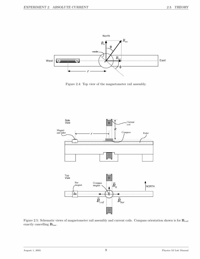
When the magnetometer rail is oriented as shown inFig. 2.4, perpendicular to the Earth’s horizontal mag-netic field Bh, the compass magnet points in the direc-tion of the net horizontal vector sum of the Earth’s fieldand that of the bar magnet. Accordingly, the angle ofdeflection φ is given by

tanφ = Bbar/Bh (2.4)

Combining equations (2.3) and (2.4), we obtain anexpression for the ratio M/Bh :

M

Bh=

2πµ0r3

(1− b2

r2

)2

tanφ (2.5)

By measuring the angle φ for a variety of distancesr (on both sides) we obtain a best estimate of the ra-tio M/Bh. If we knew the value of Bh, we would bealmost finished, since the dipole moment and there-fore the magnetic field Bbar would be known. However,the Earth’s magnetic field is highly spatially variable,especially in a building environment filled with ferro-magnetic materials, so we only know its value roughlyin advance. Measuring b and the oscillation frequencyof the bar magnet in Earth’s field gets us around thisproblem.

When the bar magnet is immersed in the Earth’smagnetic field, it experiences a torque, given by τ =M × Bh. Note that the magnitude of the torque isproportional to the product MBh. Once we know boththe product and the ratio of M and Bh, we know theirseparate values, since M =

√(M/Bh) (MBh).

If suspended by a thread of negligible torsion, themagnet will oscillate back and forth under the restoringtorque of the magnetic field. The magnet’s equation ofmotion is given by

Id2θ

dt2= −MBh sin θ (2.6)

where I is the rotational moment of inertia of the barmagnet about its center. This is the same equationthat governs a pendulum. For oscillations of small am-plitude, the oscillation frequency f is related to M Bh

by the expression

MBh = 4π2f2I (2.7)

Once M and Bh have been determined, the final re-sult of the experiment can be obtained. KnowingM , wecan use (2.3) to calculate Bbar at any distance r. For avariety of current values i (both positive and negative),we have measured the distance r at which the compassdeflection is zero, at which point |Bbar| = |Bcoil|. Thenfrom (2.2) we obtain i, a measurement of the currentwhich we have obtained without reference to externalelectrical standards.

Physics 53 Lab Manual 8 August 1, 2005

EXPERIMENT 2. ABSOLUTE CURRENT 2.3. THEORY

Figure 2.4: Top view of the magnetometer rail assembly.

Figure 2.5: Schematic views of magnetometer rail assembly and current coils. Compass orientation shown is for Bcoil

exactly cancelling Bbar.

August 1, 2005 9 Physics 53 Lab Manual

2.4. EXPERIMENTAL EQUIPMENT AND PROCEDURES EXPERIMENT 2. ABSOLUTE CURRENT

magnetometerrail

compasscurrent coil

power supply

Figure 2.6: Photograph of the magnetometer apparatus.

2.4 Experimental Equipment and Procedures

2.4.1 Preliminary setup

Figure 2.5 shows another layout view of the mag-netometer rail. As seen in the photo of Fig. 2.6, thescale on the side of the rail and the scribe mark on theside of the plastic magnet holder allow the distance rbetween the magnet and rail centers to be measured.Throughout the experiment, all superfluous magnetsand magnetic materials should be removed from thevicinity of the apparatus. Carefully orient the rail per-pendicular to the ambient magnetic field, so that theindicator needle reads zero degrees and is parallel tothe rail axis. The position of the rail on the laboratorybench should be marked with tape so that it can bereturned to the same position when it has to be movedlater in the experiment.

Before taking data, you should as always familiarizeyourself with the equipment and take some importantpreliminary measurements. After selecting a bar mag-net to use, mark its poles so that you always use it inthe same orientation throughout the experiment. (Youshould also identify the magnet you are using if you needto use the same one the following week. As a courtesyto the other students, please try not to drop or dam-age the magnets in any way that would require them toretake their data from the previous week! )

To determine the true magnetic center of your mag-net, compare the distances r measured on the right andleft sides of the compass where the compass deflection is45. If these distances differ slightly (as they probably

will), the magnet’s effective center is offset from its ge-ometric center. You should carefully record this offsetdistance and use it during the rest of the experiment tocorrect all your measured values of r.

2.4.2 The Current coil

In this part of the experiment, current from a vari-able source is connected to the circular coil. If you havenot already done so, you should determine the numberN and radius R of the coil’s turns, for use in (2.2).

Note: Large and potentially hazardous electric cur-rents are employed in this part of the experiment. Re-read Appendix A on this topic!

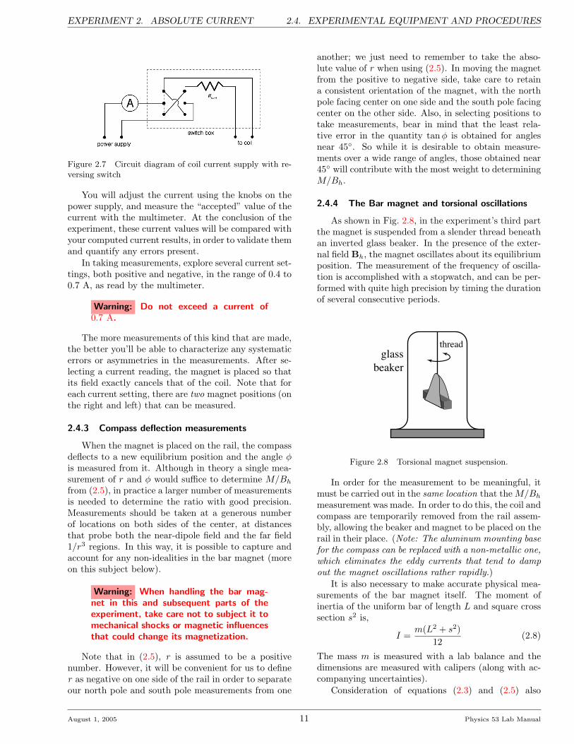
The circuit used to supply the current to the mag-net coils is shown in Fig. 2.7. The reversing switchallows you to change the direction of current, so thatyou can perform trials with the magnetic field pointingin both directions. To protect this switch from arc-ing damage, please reduce the current to zero beforereversing direction. The load resistor is located insidethe switch box, and its purpose is to limit the currentflowing in the circuit. Make sure that the meter (la-beled “A” in the diagram) is set to ammeter mode. Inorder to minimize the effects of stray magnetic fields,the switch box, the multimeter and power supply shouldbe kept several feet from the compass, and twisted pairwire leads are used to connect the coil to the supplyand switch box.

Physics 53 Lab Manual 10 August 1, 2005

EXPERIMENT 2. ABSOLUTE CURRENT 2.4. EXPERIMENTAL EQUIPMENT AND PROCEDURES

Figure 2.7 Circuit diagram of coil current supply with re-versing switch

You will adjust the current using the knobs on thepower supply, and measure the “accepted” value of thecurrent with the multimeter. At the conclusion of theexperiment, these current values will be compared withyour computed current results, in order to validate themand quantify any errors present.

In taking measurements, explore several current set-tings, both positive and negative, in the range of 0.4 to0.7 A, as read by the multimeter.

Warning: Do not exceed a current of0.7 A.

The more measurements of this kind that are made,the better you’ll be able to characterize any systematicerrors or asymmetries in the measurements. After se-lecting a current reading, the magnet is placed so thatits field exactly cancels that of the coil. Note that foreach current setting, there are two magnet positions (onthe right and left) that can be measured.

2.4.3 Compass deflection measurements

When the magnet is placed on the rail, the compassdeflects to a new equilibrium position and the angle φis measured from it. Although in theory a single mea-surement of r and φ would suffice to determine M/Bh

from (2.5), in practice a larger number of measurementsis needed to determine the ratio with good precision.Measurements should be taken at a generous numberof locations on both sides of the center, at distancesthat probe both the near-dipole field and the far field1/r3 regions. In this way, it is possible to capture andaccount for any non-idealities in the bar magnet (moreon this subject below).

Warning: When handling the bar mag-net in this and subsequent parts of theexperiment, take care not to subject it tomechanical shocks or magnetic influencesthat could change its magnetization.

Note that in (2.5), r is assumed to be a positivenumber. However, it will be convenient for us to definer as negative on one side of the rail in order to separateour north pole and south pole measurements from one

another; we just need to remember to take the abso-lute value of r when using (2.5). In moving the magnetfrom the positive to negative side, take care to retaina consistent orientation of the magnet, with the northpole facing center on one side and the south pole facingcenter on the other side. Also, in selecting positions totake measurements, bear in mind that the least rela-tive error in the quantity tanφ is obtained for anglesnear 45. So while it is desirable to obtain measure-ments over a wide range of angles, those obtained near45 will contribute with the most weight to determiningM/Bh.

2.4.4 The Bar magnet and torsional oscillations

As shown in Fig. 2.8, in the experiment’s third partthe magnet is suspended from a slender thread beneathan inverted glass beaker. In the presence of the exter-nal field Bh, the magnet oscillates about its equilibriumposition. The measurement of the frequency of oscilla-tion is accomplished with a stopwatch, and can be per-formed with quite high precision by timing the durationof several consecutive periods.

glassbeaker

thread

Figure 2.8 Torsional magnet suspension.

In order for the measurement to be meaningful, itmust be carried out in the same location that theM/Bh

measurement was made. In order to do this, the coil andcompass are temporarily removed from the rail assem-bly, allowing the beaker and magnet to be placed on therail in their place. (Note: The aluminum mounting basefor the compass can be replaced with a non-metallic one,which eliminates the eddy currents that tend to dampout the magnet oscillations rather rapidly.)

It is also necessary to make accurate physical mea-surements of the bar magnet itself. The moment ofinertia of the uniform bar of length L and square crosssection s2 is,

I =m(L2 + s2)

12(2.8)

The mass m is measured with a lab balance and thedimensions are measured with calipers (along with ac-companying uncertainties).

Consideration of equations (2.3) and (2.5) also

August 1, 2005 11 Physics 53 Lab Manual

2.5. EXPERIMENTAL ANALYSIS EXPERIMENT 2. ABSOLUTE CURRENT

shows that it is necessary to determine the distance2b between the effective poles of the magnet. There aredifferent possible approaches to getting this quantity.A simple preliminary approach is to estimate the posi-tions of the poles visually using small compasses, andmeasure the distance 2b between them with a ruler.This approach will give a fairly good “ballpark” value

for initial estimates, but often systematically differs byseveral millimeters from the results of mathematicallyfinding the best fit to (2.5). Measure and record thisprovisional value for b by this method, but keep in mindthat a better value will be obtained in later analysis bydetermining b to best fit the data with (2.9) below.

2.5 Experimental Analysis

The principal goal of this experiment is to calculatethe current i in the coil as accurately as possible, andto compare these calculations to the “accepted” valueread from the multimeter.

Perhaps the most significant challenge here is in dis-tilling the best value of M from all of the rail measure-ments. You should first carry out a quick “ballpark”calculation to verify that your results make sense, be-fore getting too deeply into the detailed analysis. It isat this stage that it is usually easiest to catch a simplemistake, such as incorrect unit conversion or a missingfactor of 2, etc. You should set up an organized spread-sheet to help with the analysis.

Pick a single representative measurement of r vs. φnear ∼ 45 and using (2.5), get a provisional value ofM/Bh. Then using (2.7), get a provisional value forM Bh; you can defer any error propagation until later,since your purpose here is to perform a quick check.If everything is correct up to this point, the dipolemoment M should be on the order of 0.5 − 1.0 Am2

and the horizontal magnetic field Bh should be roughly2×10−5 T. If your results are not in this range, go backand find the mistake before proceeding further. Finally,set equations (2.2) and (2.3) equal to one another us-ing your provisional values for M and b to obtain thecurrent i for one of your trials in the first part of theexperiment. If all is well, it should agree with the mul-timeter reading within about 10% or so. Next we’lldiscuss how the final analysis will hopefully refine thisresult.

The simplest approach would be to simply obtainseparate estimates of M/Bh from (2.5) for every mea-surement, and then take their average. However, thisapproach has some disadvantages. Some of the impor-tant sources of error, such as errors in the pole spacingb for example, tend to systematically push the M/Bh

estimate off in one direction, rather than randomly. Asa result, averaging over a lot of measurements yields aresult that retains a bias from the “true” value, thatcannot be averaged out.

A more sophisticated and potentially better ap-proach is to fit the expression of (2.5) to the unknownparameters M/Bh and b, given the experimental mea-surements of φ vs. r. Solving the expression for φ, wewant to fit the experimental data to the function,

φ = arctan

µ0

2π(M/Bh)

|r|3(1− b2

r2

)2

(2.9)

Using a plotting/fitting computer utility such asOrigin or Kaleidagraph and proper error weighting, youcan solve for the unknowns M/Bh and b, as well astheir uncertainties. Fig. 2.9 shows schematically howwe might expect this fit to look when plotted.

80°

60°

40°

20°

f

100806040200

Magnet Position (cm)

Eq. (2.9)

Figure 2.9 φ vs. r data fitted to (2.9).

2.5.1 Fitting

The use of a plotting program to perform such aparameter fit is a great labor-saving convenience, andpretty easy. However, it pays to be familiar with thesoftware and how it works before you need to use it.Here are some hints and reminders for using Kaleida-graph and Origin to analyze this experiment:

Kaleidagraph

When defining your fitting function, Kaleidagraphrequires the independent variable (i.e., r) to be namedm0. It requires the parameters (i.e b and M/Bh) to benamed m1 and m2 (and so on). So with the program setto compute in degrees (rather than radians), the defini-tion of your fitting function should look something likethis:

invtan(m2/(5e6*abs(m0^3)*(1-(m1/m0)^2)^2));

m1=0.03;

m2=32000

Physics 53 Lab Manual 12 August 1, 2005

EXPERIMENT 2. ABSOLUTE CURRENT 2.5. EXPERIMENTAL ANALYSIS

Note that it is necessary to provide the initial guessvalues following the function definition, or the programwon’t be able to get a solution. Also remember that youmust specify a weighted fit, or else the χ2 goodness-of-fit figure you obtain will be meaningless. In Kaleida-graph, you need to divide this number by the number ofdegrees of freedom (# of data pts. – # of parameters)in order to get χ2 per degree of freedom.

Origin

When defining your fitting function, Origin allowsyou to name the parameters whatever you like. Forsimplicity here, we will use the names b and M andcall the independent variable R. Origin works only inradians, so we must convert into degrees. The fittingfunction definition for Origin would look like:

(180/pi)*atan(M/(5e6*abs(R^3)*(1-((b^2)/(R^2)))^2))

Origin also requires you to provide starting guessvalues for the fitting parameters, but these are speci-fied in the ‘Start Fitting Session’ dialog, rather than inthe function definition. In Origin, the reported χ2 valueis already normalized to χ2 per degree of freedom.

Igor

Like Origin, Igor allows you to name the fit param-eters anything you like. For simplicity here, we will usethe names b and M and call the independent variabler. Igor works only in radians, so we must convert intodegrees. The fitting function definition for Igor wouldlook like:

f(r) = (180/pi)*atan(M/(5e6*abs(r^3)*(1-((b^2)/(r^2)))^2))

Igor also requires you to provide starting guess val-ues for the fitting parameters, but these are specifiedin the ‘Coefficients’ pane of the fitting dialog. Igor re-ports the value of χ2, so if you would like the reducedχ2 value, divide by the number of degrees of freedom.

All

In all cases the fitting programs do your error anal-ysis for you automatically. The fitted values of the pa-rameters are reported along with their propagated un-certainties. However, before you use these values uncrit-ically, remember that these uncertainties are only validto the extent that the residuals of the fit are randomlydistributed and χ2 per degree of freedom for the fit isapproximately unity. See http://www.physics.hmc.edu/analysis/fitting.php for more information.

August 1, 2005 13 Physics 53 Lab Manual

Experiment 3RLC Resonance

Abstract

Current in a series circuit comprising a resisitor, capacitor, and inductor tends to oscillate at afrequency that depends on the inductance L of the inductor and the capacitance C of the capacitor,although resistance damps out the oscillations. You will study how the oscillating current generatedby an applied AC voltage depends on frequency, observing the maximum response (resonance) at thenatural frequency set by L and C.

3.1 Overview

When you push a child on a swing, the amplitude ofthe child’s motion builds up swing by swing: with eachpush you pump energy into the child-swing system. Un-less you are warped, you tend to push the child at thenatural frequency, which is the frequency at which thesystem oscillates when you stop pushing and the childswings by herself.

In this experiment, you get to be warped and pushat all sorts of frequency, from the pathetically low tothe ridiculously high. Between these extremes lies thenatural frequency, the one the system likes the best, as

judged by the amplitude of the motion it experiences.In the case of the swing, it’s the child that moves. Inan RLC circuit, it’s the electric current. To help yougain an intuition for the three circuit elements involved,they are introduced in Fig. 3.1.

1. Before lab — Read this chapter of the lab man-ual. The theoretical introduction is significant,so devote adequate time to understanding it. Itwill make your experience in lab much easier. Ifneeded, you may read HRK Chapter 37 for more

Element Equation Properties

R VR = IR

A resistor is a piece of poorly conducting wire, a pipe throughwhich electric current flows. The magnitude of the current de-pends on the voltage across the resistor: double the voltage andyou double the electric current. The mechanical analog of a resis-tor is a viscous liquid, like honey, through which you are trying topush an object. Resistors turn good, clean electrical energy intoheat, a process that is called Joule heating.

C VC =Q

C

A capacitor is a pair of conducting plates facing one another acrossa gap. Electric charges flowing onto one plate produce an electricfield in the gap between the plates, causing the voltage of oneplate to differ from that of the other. The mechanical analog of acapacitor is a spring: as you pile up charge, it creates an electricforce that makes it harder to pile up more charge. Note, however,that as the capacitance C increases, it becomes easier to pile upcharge: a bigger capacitor behaves like a softer spring. As chargebuilds up, capacitors store energy in the electric field between theirplates.

L VL = LdI

dt

An inductor is a coil of wire. As current flows in the coil, it gener-ates a magnetic field inside the coil, which opposes a further changein the current. The mechanical analog of inductance is mass, whichopposes a change in the state of motion. The greater the induc-tance L, the more the inductor opposes a change in the currentthat flows through it. Inductors store energy in the magnetic fieldgenerated by the current flowing through them.

Figure 3.1: Basic properties of resistors, capacitors, and inductors.

Physics 53 Lab Manual 14 August 1, 2005

EXPERIMENT 3. RLC RESONANCE 3.2. THEORY

detail.

2. Choose a specific experiment option in consulta-tion with your instructor.

3. You must analyze the results and present a rigor-ous discussion of your findings. Often, the experi-

ence gained (and mistakes made) during the firstweek’s meeting will allow you to be that muchmore efficient and effective in completing the ex-periment the following week.

3.2 Theory

Resonance is a ubiquitous and very important phe-nomenon in physics, which is not restricted to electroniccircuits. “Pumping” a swing and tuning a radio areboth examples you are familiar with (although you maynot have realized you were “resonating” at the time!).The key feature of all resonance effects is that the sizeof the effect (for example, the height the swing goes orthe volume of the the sound) depends on the frequencyof the excitation. Several Nobel Prizes in physics havebeen awarded over the years for studies of resonance— for example, nuclear magnetic resonance (the basisof magnetic resonance imaging, or MRI, an importantmedical tool of recent vintage). In this experiment youwill study the phenomenon of resonance in a simple AC(alternating current) electrical circuit.

The electrical circuit you will study comprises a re-sistor, a capacitor, and an inductor. The resonanceeffect in this experiment stems from the fact that thevoltage drop across the individual circuit elements de-pends on the frequency of the sinusoidal voltage appliedto the circuit. In some cases, the voltage drop can be oflarger magnitude than the applied voltage (just as theswing can go much farther than you push it, given theright frequency). To understand this effect, we beginwith the basics of elements in an AC circuit, and howtheir frequency-dependent behavior is mathematicallydescribed.

Briefly, the three topics we should understand forthe purposes of this experiment are:

• AC voltages represented as complex numbers(what are amplitude and phase?)

• Impedance of discrete circuit elements (relation-ship between voltage and current)

• Analyzing a circuit with more than one element(how to apply the Kirchhoff laws)

3.2.1 AC voltages as complex numbers

A steady AC voltage is represented as a sinusoidalfunction of time, with a fixed amplitude, frequency andphase shift. We will call the the amplitude V0, the

phase φ, and the angular frequency ω (ordinary fre-quency ν = 1/T = ω/2π). Therefore, we write thetime-dependent voltage as

V = V0 cos(ωt+ φ) = V0 Re[ei(ωt+φ)

](3.1)

In the latter half of the above equation, we make useof Euler’s identity to express the sinusoid in terms ofcomplex exponentials. In this notation the imaginaryunit is i and the real part of the expression gives us thecosine part.1 At first this seems an unfriendly compli-cation, but upon reflection we see that the exponentialexpressions are much easier to manipulate algebraicallythan sines and cosines. In practice, we typically leavethe taking of the real part as tacitly understood, and justleave the expression in its complex form: V0e

i(ωt+φ).If we assume that the only time dependence in the

system is in the sinusoidal voltage at ω (that is, the sys-tem is in steady state), our expressions simplify evenfurther. Then without any loss of generality we cansimply factor out the time dependence in the expres-sions, and focus our attention on the amplitude andphase of the voltage. Schematically we have replacedreal voltages with a complex number as in,

V = V0eiφ (3.2)

We can perform all needed calculations using thiscomplex representation. When working with a quan-tity like (3.1) that has explicit time dependence, theobservable instantaneous voltage is always obtained bytaking the real part. When we leave out the time de-pendence as in (3.2), the absolute value of the complexnumber tells us its amplitude, while the argument orphase tells how much the sinusoid lags or leads in itscycle relative to the cosine function.2

This algebraic representation of the voltage has ageometrical analog called a phasor diagram. A phasoris a vector in the complex plane whose magnitude is theamplitude of the voltage and whose direction gives thephase.3 For example, we show the phasor diagram foran AC voltage in Fig. 3.2. In the illustrated case, theangle the phasor makes with the real axis is just ωt; ifthe waveform were delayed in phase by an amount φ(as it is in (3.1)), then this angle would be ωt− φ.

1Note that engjneers sometjmes use j =√−1 as the jmagjnary unjt, presumably so jt wjll not be confused wjth electrjcal current.

2Recall that if a complex number z = x + iy is not already expressed in polar form, its absolute value and argument are given byA = |z| =

px2 + y2 and φ = arg(z) = arctan(y/x). So x + iy = Aeiφ in this example.

3The “arrows” Feynman uses in QED to discuss photons are phasors that represent the complex probability amplitude.

August 1, 2005 15 Physics 53 Lab Manual

3.2. THEORY EXPERIMENT 3. RLC RESONANCE

ωtRe

Voeiωt

Im

Re[V] = Vocosωt

Figure 3.2 Phasor representation of a sinusoidally varyingvoltage at time t. The actual measured voltage is the pro-jection of the phasor on the real axis.

The locus of points traced out by the phasor as afunction of time is a circle as shown in Fig. 3.3. Thetrue voltage oscillates between ±V0.

t

V

Vocos(ωt)

Vo

ωt

Figure 3.3 Time dependence of relationship between pha-sor representation and real observed sinusoidal voltage.

Now consider two AC voltages, both at the samefrequency, as shown in Fig. 3.4. The voltages have dif-ferent phases. In Fig. 3.4 (a), the phase difference isshown as the angular separation of the phasor vectors.In Fig. 3.4 (b) this phase difference is appreciable in thedifferent instantaneous magnitudes of the two voltages,even though they have the same amplitude.

t

V

A

AB

B

Im

Re

Vo

Figure 3.4 Relationship between phasors of different phase.

3.2.2 Complex impedance

Impedance is just a slight generalization of the con-cept of resistance, with which you are already familiarin the context of Ohm’s law, (1.2). Just as in the case

of the resistance of a resistor, impedance is the ratioof voltage to current for a given element, be it a re-sistor, capacitor, or inductor. In general, this differsfrom resistance because the ratio of voltage to currentmay depend on frequency, and because there may bea phase difference (lag or lead) between the sinusoidalvoltage and current. For this reason, the impedance ofa circuit element is in general a number with both mag-nitude and phase (a complex number) and depends onfrequency (rather than being a fixed constant). In gen-eral we define impedance Z by the relation, V = IZ,where all the quantities may be complex. If for exampleV and I have different phases, then

V = V0eiφ1 and I = I0e

iφ2 (3.3)

imply that

Z =V0

I0ei(φ1−φ2) (3.4)

Impedance of a resistor

This is the simple and familiar case of Ohm’s law.As we discussed above, for a pure resistor there is nophase lag or frequency dependence, so the impedancereduces to the simple (real) result,

VR = IR implies ZR = R (3.5)

Thus the impedance for a resistor is just same as its DCresistance.

Impedance of an inductor

The relationship between the voltage and currentfor an (ideal) inductor is

VL = LdI

dt(3.6)

Applying the complex representation of the AC voltageand current, this becomes,

VLeiωt = iωLIeiωt or VL = iωLI (3.7)

Thus the impedance for an inductor is

ZL = iωL (3.8)

If the current is assumed real across an inductor(cosine-like) then the corresponding voltage is purelyimaginary (sine-like), or different in phase by 90. Also,we see that for low frequencies an inductor presents lit-tle obstruction to the flow of current, but at large ω ittakes a large voltage to cause current to flow; hence,the inductor will then act somewhat like a large resis-tor, neglecting phase effects. We say that an (ideal)inductor is a “short circuit” at low frequency and an“open circuit” at high frequency.4

4The inductor(s) you will use differ from an ideal inductory in two important respects. First, because it takes many turns of wire toproduce a significant inductance, the wire of the inductor is fairly fine. This means that it has nontrivial resistance, is shown schematicallyin Fig. 3.5.

Physics 53 Lab Manual 16 August 1, 2005

EXPERIMENT 3. RLC RESONANCE 3.3. EXPERIMENTAL PROCEDURE

Impedance of a capacitor

The relationship between voltage and current for acapacitor is

VC =Q

C=

∫I dt

C(3.9)

Again, going to complex representation we find,

VCeiωt =

Ieiωt

iωCor VC =

I

iωC

Thus, the impedance for the capacitor is

ZC =1iωC

= − i

ωC(3.10)

We see that the voltage and current of the capacitoralso differ in phase by 90, but in the sense opposite tothat of the inductor. The capacitor is also opposite tothe inductor in that it presents the greatest obstacle tocurrent flow at low frequencies, and little obstructionas ω grows large. A capacitor is an “open circuit” atlow frequency and a “short circuit” at high frequency.Much insight into asymptotic behavior can be achievedby considering these components to be large or smallresistors in the appropriate frequency limit.

These are the basic concepts to understand; the de-tailed use of these impedances to derive the behavior ofan RLC circuit is found in Sec. 3.4.

3.3 Experimental Procedure

3.3.1 Equipment and software

Having covered the theory behind this experiment,we now turn our attention to the equipment you willuse to carry it out. Although in principle you couldmeasure all the needed voltage amplitudes and phasesmanually with an oscilloscope, this would be very te-dious and limit the amount of data you could take in areasonable time. Instead, you have an Igor-based com-puter data acquisition system which greatly simplifiesthe procedure.5

The computer acquisition system has four analogsignal input channels; one for the driving voltage andthe remaining three for the voltages across the threecircuit components (R, L, and C). The application in-terface provides a virtual oscilloscope window, in whichyou can view up to all four waveforms simultaneouslyin real time. In addition to displaying the waveforms,the program displays the frequency of the applied sinu-soidal voltage signal, as well as the amplitude and phaseof the voltages across the resistor, inductor, and capac-itor (measured with respect to the driving voltage). Aconsistent color scheme is used throughout: the drivesignal is black, and the resistor, inductor, and capaci-tor are represented by red, green, and blue, respectively(RLC → RGB).

The application also produces plots of the ampli-

tude/phase results, and exports the data for use in othergraphing and analysis programs. Within the Igor ap-plication, you can view or print graphs of amplitudeand phase vs. frequency on either linear or logarith-mic axes. The application can superimpose theoreticalcurves for the RLC circuit [as described in equations(3.16), (3.18), and (3.20)]. There is also an option toplot data and theory in phasor form on the complexplane. More detailed step-by-step instructions on theuse of the program are provided at the end of this sec-tion.

In addition to the computer equipment, you are pro-vided with a variety of components and hook-up wireswith which to construct your circuit and connect it tothe computer. Figure 3.5 shows a schematic diagram ofthe arrangement of components for the standard RLCcircuit measurement. Attention should be paid to ob-serving the correct polarity in the connection of thecomputer input channels; if reversed the resulting volt-age will be negative and therefore 180 out of phasewith theory. Also note that you are provided with fourdigital multimeters, which when hooked up in parallelwith each channel provide valuable additional diagnos-tic information. Note that in AC voltage mode, themultimeters report the root-mean-square voltage, notthe peak-to-peak voltage, which is twice the amplitude.

The second nonideality of the inductor arises from its ferromagnetic core. To enhance the inductance of a coil one can fill the openspace inside the coil with a ferromagnetic material, typically iron. Because of hysteresis in the iron, the inductor in this experimentresponds somewhat nonlinearly to the current. The significance of this effect depends on both the amplitude and frequency of the drivevoltage. Exploring this nonlinearity can be a fruitful avenue for a technical report.

5 Igor is a powerful data acquisition, analysis, and graphics program that runs on both Macintosh and Windows. Unlike Kaleidagraph,Igor is entirely scriptable: virtually everything that can be accomplished using the graphical user interface can be programmed within Igorusing a C-like programming language. The programs that acquire and analyze data for the RLC and Fraunhofer diffraction experimentsproduce Igor experiment files holding your data, graphs, and tables, as well as a history of the operations you conduct. You may usethem to export data in text format for further analysis in Kaleidagraph, Origin, or other program, or you may analyze your data furtherwithin Igor. See http://www.physics.hmc.edu/analysis/Igor.php for further information about using Igor.

August 1, 2005 17 Physics 53 Lab Manual

3.3. EXPERIMENTAL PROCEDURE EXPERIMENT 3. RLC RESONANCE

f V1

V2

V3

V4

Computer InputChannel 1

Computer InputChannel 2

Computer InputChannel 3

Computer InputChannel 4

L

R

C

RL

Figure 3.5: A series RLC circuit driven by an oscillating voltage. The voltmeters shown as circles are the digitalmultimeters. The boxes showing channels are the connections to the analog-to-digital converter in the computerallowing the computer to function as an oscilloscope. The (unavoidable) internal resistance of the inductor is shownexplicitly.

Choosing an Experiment

This experiment provides you with the choice of sev-eral options to pursue. Depending on your particularinterests and previous electronics experience, you mayfind one of the options more attractive than the others.The following description details the procedure for thestandard experiment option, followed by descriptions ofother possible alternative experiments. You will prob-ably have time to do more than one.

(a) Standard option: series RLC circuit

Construct a series RLC circuit like the one shown inFig. 3.5. The usual nominal values to use for the capac-itance and inductance are C = 5 µF and L = 500 mH.With these values fixed, you will repeat the measure-ments twice for two different values of the resistance,R = 50 Ω and 500 Ω. Note that you can readily use oneof your digital multimeters to directly measure the ac-tual values of the resistances R andRL. It is a good ideato do this before assembling the series circuit. However,the actual values of L and C may differ from their nom-inal manufacturer’s values, so one of your objectives inthis experiment will be to extract from your results re-fined estimates of these component values. Pay atten-tion to the polarity of the banana-to-BNC connec-tors: the outside conductor on the BNC cable goesto the marked side of the banana jacks. What mighthappen if you reverse the polarity?

Using the Igor application, collect amplitude andphase data for each of the components. Vary the input

frequency from the function generator over the rangeof roughly 20 to 900 Hz. You can monitor the dataas you collect it on either a linear or logarithmic fre-quency scale in the data window (see Fig. 3.8). Youcan also superimpose theoretical curves. Unless youhave made a mistake somewhere, your amplitude andphase results should appear quite close to the theoret-ical curves using the nominal values of R, L, C, andRL. Compare and contrast the results you get for thetwo different choices of the damping resistor, R. In par-ticular, try to estimate the sharpness of the resonancepeak with the “quality factor” defined as Q = ω0/∆ω,where ω0 = 1/

√LC is the resonant (peak) frequency

and ∆ω is the peak’s full width at half-maximum. Alittle algebra shows that the quality factor of the volt-age resonance should be related to total resistance, L,and C through

Q =ω0L√

3(R+RL)(3.11)

Check the consistency of your experimentally deter-mined values of Q and ω0. The culmination of youranalysis will be in determining the best values of L andC consistent with your data. Although you could try aseries of trial-and-error guesses for the values in ques-tion, this approach can be tedious and unwieldy.

The preferred approach is to use “inverse model” orfitting techniques. Igor is a very powerful data analysisenvironment with a very flexible nonlinear least squaresfitting procedure built in. For the functions of the series

Physics 53 Lab Manual 18 August 1, 2005

EXPERIMENT 3. RLC RESONANCE 3.3. EXPERIMENTAL PROCEDURE

RLC circuit, the necessary fitting functions are alreadydefined for you. Using the Fit pop-up menu in the datawindow, you can fit each of the six data sets (amplitudeand phase for the resistor, inductor, and capacitor) toequations (3.16), (3.18), and (3.20). Note that for manyof these fits, the value of R and RL are redundant: onlytheir sum matters. You will need to hold fixed at leastone of the resistances to obtain reasonable results.

The validity of the fitting procedure is an open ques-tion, for reasons that are discussed in Sec. 3.6. A goodway to estimate the confidence with which a circuit pa-rameter is determined by fitting is to compare the valueobtained by fitting to different data. For example, dofits to the inductor phase and the inductor amplitudeyield similar values for L? Are the residuals shown atthe top of the fit window randomly distributed, or dothey exhibit systematic errors? Explore your data anddiscuss your observations and conclusions in your note-book. Note that it is unnecessary to print each andevery fit graph. Pick one or two representative graphsto print. Cut the two copies on the dashed line, tape acopy into your notebook, and write a brief discussion ofits salient features and your conclusions about the ex-tent of agreement or disagreement between your dataand the linear theory of a series RLC circuit.

(b) Parallel RLC analysis option

This option may appeal to students who enjoy themathematical or theoretical side of things. Construct acircuit as in the standard option, but instead of a seriescircuit, connect two of the three elements in parallelwith one another and the third element in series withthat pair. Which of the three elements, R, L, or C, tomake the series element is up to you; making the resis-tor the series element [R(L||C)] is a choice that leadsto a particularly interesting resonance behavior. Thetheory of the parallel-series circuit is not derived in thislab manual, although the method to do so is similar.The challenge of this option is to derive the appropri-ate equations describing your chosen circuit, and thencompare them with experimental data you take for asingle choice of R, L, and C. To keep the amount ofwork to a reasonable level, only derive the voltage am-plitude and phase for the single series element.

After gathering data for your circuit, use the Plotbutton of the data window (Fig. 3.8) to extract andplot either the amplitude or phase data from one of thechannels. A new plot window with these data is cre-ated, which you can use for fitting. To begin the fitting

procedure, with the plot window frontmost select Anal-ysis | Curve Fitting. . . and be sure to check the FromTarget box. See the Igor web page at http://www.physics.hmc.edu/analysis/igor.php for more infor-mation on using Igor for fitting data. You may alsoexport the data in text form for fitting in another pro-gram, such as Kaleidagraph. Click the Save button inthe data window to do this.

One word of caution in constructing fitting functionsfor phases. Inverse trigonometric functions are multiplevalued. You may need to add or subtract 180 in somecases.

(c) Unknown “black box” determination option

For those who find the standard experiment optiona little too cut-and-dried, this option provides a lit-tle “mystery.” Your instructor has a number of sealedboxes that contain a resistor, inductor and capacitorconnected in series inside. In addition to the two endterminals (to which you connect the driving voltage),there is a pair of test terminals that gives you accessto the voltage across one of the unknown components(you’re not told which one of the three). In additionto measuring the DC resistance across any pair of thefour terminals, you gain information about this systemby driving it with voltages of various frequencies, andusing the computer system to measure and record theamplitudes and phases across the test terminals. Donot drive the system with voltages greater than 0.1 Vor the inductors will not act as linear devices.

Using the methods and theory described above, youshould be able to deduce the values of L, C, R and RL

inside the box, and which of the three components thetest terminals are connected to. When using the com-puter to assist you in fits of your data, it is best to fixthe value of R since you have measured it directly andthe fit is not tightly constrained otherwise. You mayhave time to analyze more than one unknown box.

(d) Design your own experiment option

Using your own ideas and/or ideas from the abovethree options, you may want to devise your own customexperiment. It should use the basic methods and ap-paratus of the experiment as described above, but mayemphasize some different aspect or circuit design thatyou find particularly interesting. Consult with your in-structor for his or her approval of your experimentalplan.

August 1, 2005 19 Physics 53 Lab Manual

3.4. ANALYZING A CIRCUIT WITH MORE THAN ONE ELEMENT EXPERIMENT 3. RLC RESONANCE

3.4 Analyzing a circuit with more than one element

The payoff for our development of the ideas of com-plex impedance is realized now in the ease with whichwe can analyze circuits consisting of combinations ofthese three elements. Series and parallel impedancesadd in a manner exactly analogous to DC resistances.As a result, analyzing a circuit composed of inductors,capacitors and resistors is no harder conceptually thandealing with the same circuit composed of all resistors.

As an illustration, we’ll look at the series RLC cir-cuit and compare it with a series circuit of three resis-tors, as illustrated in Fig. 3.6.

The analogous resistor circuit is quite easy to an-alyze. The current through each resistor must be thesame, and follows from the series resistance of the three,

I =V0

R1 +R2 +R3(3.12)

Since the three resistors form a simple voltage divider,we can also easily write the voltage drop across eachone,

V1 = V0R1

R1 +R2 +R3

V2 = V0R2

R1 +R2 +R3

V3 = V0R3

R1 +R2 +R3

Now we apply the same reasoning to the series RLCcircuit. In this case the current through each elementof the circuit is given by,

I =V0

ZR + ZL + ZC(3.13)

Now in this case, the impedances are not all real,so we expect that the resulting current I will be some

amount out of phase with the driving voltage. The volt-ages across each of the elements are now simply givenby,

VR = V0ZR

ZR + ZL + ZC

VL = V0ZL

ZR + ZL + ZC

VC = V0ZC

ZR + ZL + ZC

We must take note of the fact that by virtue of theirconstruction as coils of wire, inductors generally have anon-negligible resistance, in addition to their designedinductive impedance. As a result, we have to replacethe expression in equation (7) with one that takes thefinite resistance of the inductor into account:

ZL = iωL+RL (3.14)

In this expression, RL is the resistance in ohms of the in-ductor that would be measured at DC (ω = 0). Armedwith these expressions, we can now predict all of thevoltages and phases across every element of our circuit.For the resistor, we obtain,

VR = V0R

R+ iωL+RL + −iωC

(3.15)

which yields the amplitude and phase (lag),

|VR| = V0R√

(R+RL)2 +(ωL− 1

ωC

)2

φR = arctan( 1

ωC − ωL

R+RL

)(3.16)

For the inductor, we obtain,

VL = V0iωL+RL

R+ iωL+RL + −iωC

(3.17)

I

R

C

L

RL

V0eiωt

(a) AC circuit

I

R1

R2

R3

Vo

(b) Resistor circuit

Figure 3.6: (a) An RLC circuit shown driven by an oscillating voltage. (b) An analogous DC circuit composed ofthree resistors.

Physics 53 Lab Manual 20 August 1, 2005

EXPERIMENT 3. RLC RESONANCE 3.5. INSTRUCTIONS FOR USING THE IGOR RLC APPLICATION

which yields the amplitude and phase,

|VL| = V0

[R2

L + (ωL)2

(R+RL)2 +(ωL− 1

ωC

)2

]1/2

φL = arctan(ωL

RL

)+ arctan

( 1ωC − ωL

R+RL

)(3.18)

And finally, for the capacitor, we obtain,

VC = V0−i/ωC

R+ iωL+RL + −iωC

(3.19)

which yields the amplitude and phase,

|VC | = V01/ωC√

(R+RL)2 +(ωL− 1

ωC

)2

φC = arctan( 1

ωC − ωL

R+RL

)− π

2(3.20)

These derived expressions for the amplitude and thephase lag depend on frequency, and contain the math-ematical essence of the resonance phenomena you willbe observing. Although it will be up to you in the ex-periment and analysis to explore these functions, wepresent in Fig. 3.7 some typical plots to show you whatyou might expect.

1.2

1.0

0.8

0.6

0.4

0.2

0.0

V /

Vo

200150100500

f = w / 2p (Hz)

VR

VL

VC

-180°

-90°

0°

90°

180°

f

200150100500

f = w / 2p (Hz)

fC

fR

fL

Figure 3.7: Example RLC voltage amplitudes as a function of frequency. For the illustrated case, R = 100 Ω,L = 0.6 H, C = 30 µF, and RL = 40 Ω.

In pondering these equations and their graphs, youshould ask yourself the following questions:

• What is significant about the system’s responseat the resonant frequency, ω0 =

√1/LC?

• Why do VL and VC approach the limits of zeroand V0 at opposite extremes?

• What influences the width of the peak in VR, andthe “overshoot” in VL and VC?

• Why do the phases always differ from each otherby 90, except for φL as ω → 0?

• How is this system analogous to resonance of amechanical spring-mass-damper system?

3.5 Instructions for Using the Igor RLC Application

The Igor RLC application (written by HMC studentAndy Fischer (’06) and Peter N. Saeta) is designed toacquire the data for voltages as a function of time forVapplied, VR, VL, and VC . It will also calculate the nor-malized voltages and phase relative to Vapplied, and plotthem on two types of graph: V or φ versus frequencyand a phasor plot. If you enter values for R, RL, L, orC, it will calculate the theoretical values and plot them.It will also export data to a text file.

Warning: Do not tamper with the dataacquisition computer.

Warning: The program that runs this ex-periment sometimes loses mouse clickswhile it is processing the data. Hold downthe Escape key to stop the oscilloscope ifyour mouse clicks are getting lost.

The basic operation of the program is as follows:

1. Launch Igor (if it is not already running). Clickon the Igor icon in the Dock at the right of the

August 1, 2005 21 Physics 53 Lab Manual

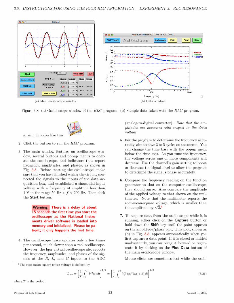
3.5. INSTRUCTIONS FOR USING THE IGOR RLC APPLICATION EXPERIMENT 3. RLC RESONANCE

(a) Main oscilloscope window. (b) Data window.

Figure 3.8: (a) Oscilloscope window of the RLC program. (b) Sample data taken with the RLC program.

screen. It looks like this: .

2. Click the button to run the RLC program.

3. The main window features an oscilloscope win-dow, several buttons and popup menus to oper-ate the oscilloscope, and indicators that reportfrequency, amplitudes, and phases, as shown inFig. 3.8. Before starting the oscilloscope, makesure that you have finished wiring the circuit, con-nected the signals to the inputs of the data ac-quisition box, and established a sinusoidal inputvoltage with a frequency of amplitude less than1 V in the range 50 Hz < f < 200 Hz. Then clickthe Start button.

Warning: There is a delay of about15 seconds the first time you start theoscilloscope as the National Instru-ments driver software is loaded intomemory and initialized. Please be pa-tient; it only happens the first time.

4. The oscilloscope trace updates only a few timesper second, much slower than a real oscilloscope.However, the Igor virtual oscilloscope also reportsthe frequency, amplitudes, and phases of the sig-nals at the R, L, and C inputs to the ADC

(analog-to-digital converter). Note that the am-plitudes are measured with respect to the drivevoltage.

5. For the program to determine the frequency accu-rately, aim to have 3 to 5 cycles on the screen. Youcan change the time base with the popup menubelow the time axis. As you tune the frequency,the voltage across one or more components willdecrease. Use the channel’s gain setting to boostor decrease the signal level to allow the programto determine the signal’s phase accurately.

6. Compare the frequency reading on the functiongenerator to that on the computer oscilloscope;they should agree. Also compare the amplitudeof the applied voltage to that shown on the mul-timeter. Note that the multimeter reports theroot-mean-square voltage, which is smaller thanthe amplitude by

√2.6

7. To acquire data from the oscilloscope while it isrunning, either click on the Capture button orhold down the Shift key until the point appearson the amplitude/phase plot. This plot, shown as(b) in Fig. 3.8, appears automatically when youfirst capture a data point. If it is closed or hiddeninadvertently, you can bring it forward or regen-erate it by clicking on the Plot Data button ofthe main oscilloscope window.

Mouse clicks are sometimes lost while the oscil-6The root-mean-square (rms) voltage is defined by

Vrms =

»1

T

Z T

0V 2(t) dt

–1/2

=

»1

T

Z T

0V 20 cos2(ωt + φ) dt

–1/2

(3.21)

where T is the period.

Physics 53 Lab Manual 22 August 1, 2005

EXPERIMENT 3. RLC RESONANCE 3.5. INSTRUCTIONS FOR USING THE IGOR RLC APPLICATION

loscope is running; you can use the Shift key fortaking data points and the Escape key to stop theoscilloscope. Note that you can take data con-tinuously by holding the shift key down as yougradually change the frequency. If you go toofast, your data will suffer because the frequencychanges during the measurement. You may alsooverload one of the channels.

8. To clear all data and start over, click the ClearData button. Note that this does not save thedata first; all unsaved data will be lost.

9. To remove points from the data, or to examine theraw numerical data, click the Edit button in theAmplitudes and Phases window. A spreadsheetwindow opens with one row for each data point.To delete a point, click in the “Row” column atthe left to select the entire row. Then use theData | Delete Points. . . command to delete thepoint(s). Note that there is no “undelete” func-tion. Any graphs that depend on these data willbe updated automatically.

10. To add theoretical curves to your data, click thePlot Theory button in the amplitude/phase win-dow. Enter the circuit parameters. The ex-pected curves (taking into account the inductorresistance) are shown superimposed on the data.(Note that this assumes a series RLC circuit. Ifyou have constructed a different circuit, you canuse the Plot menu to prepare a graph of a par-ticular data set, on which you can superimpose acurve of your own specification. See below.)

11. To fit your data to the expected theoretical ex-pressions, select the data set from the Fit pop-upmenu. Enter initial guesses for the circuit parame-ters, and check any boxes for parameters you wishheld fixed during the fitting procedure. Note thatfor many fitting operations, the value of R and RL

are redundant: only the sum of these resistancesmatters to the fit function. In such cases, youshould make sure to hold at least one resistancevalue fixed.

The fit results are shown on the plot window.Beside each parameter is either an open square(meaning the parameter was varied during the fit)or a filled square (meaning that it was held fixed).Note that the curves of the main data window areupdated to reflect the fitted values of the param-eters.

A more complete summary of the fit results isprinted to the History window at the bottom ofthe screen. The reported value of χ2 (V_chisq)is not reduced. The fits use the “measured uncer-tainties” (see below), but rarely produce a valueof χ2 consistent with a good fit. Inspect the panel

of residuals at the top of the plot window to inves-tigate the validity of the fitting procedure. Youshould also study the variation in fitted parame-ters when you hold different parameters fixed andwhen you fit a different curve of the data set.

12. When you have finished acquiring data for a givencircuit, click the Save button of the data window.This saves (1) the complete Igor experiment, (2)the current batch of data, setting its name basedon the current time, (3) a tab-delimited text ver-sion of the data with the same time stamp, (4)and an Igor binary version of the data with thesame time stamp. The text version can be readby any data analysis program on any platform.

The text file format is tab-delimited text, whichcan be opened by any data analysis package. Thefirst row holds column labels, and subsequentrows hold the data. There is a potential gotchawith text files: different operating systems usedifferent characters to indicate the end of a line.UNIX computers use the linefeed character (LF= ASCII 10), Macintosh computers use the car-riage return character (CR = ASCII 13), andDOS/Windows computers use both (CR+LF)! Ifyour data analysis program has trouble readingthe file, you can use Excel to open it first andhandle the conversion of line terminators.

To copy the data to your Charlie account, makesure you are in the Finder (check the first textitem in the menubar at the top of the screen;if it isn’t Finder, then click the first icon in theDock) and press Command-K or select Connectto Server. . . from the Go menu. Enter char-lie.ac.hmc.edu and you will be presented a logindialog.

13. If you would like to try your own fitting function(which is necessary if you have set up a circuitother than a series RLC circuit), use the Plotpop-up menu to copy the appropriate data andproduce a plot window of it. Then select Analysis| Curve Fitting. . . and be sure to select the FromTarget check box. This limits the data shown indialogs to that already in the figure. Click theNew Fit Function. . . button and enter your fitfunction. Proceed sequentially through the tabsat the top of the dialog window, entering infor-mation is necessary. In particular, make sure youenter reasonable parameter values. You may clickon the Graph Now button to see how close thedata are to the curve computed with the valuesyou have entered. When you are satisfied that itis close, click the Do It button to complete thefit. Results will be shown in the History area atthe bottom of the screen.

August 1, 2005 23 Physics 53 Lab Manual

3.6. PROGRAM DETAILS EXPERIMENT 3. RLC RESONANCE

14. The Load Data button allows you to restore a pre-viously saved data set (it must have been savedwithin the same Igor experiment, however). Se-

lect the data set you wish from the pop-up menuand it will be restored to the main data window.

3.6 Program Details

This section provides details about the internalworking of the RLC program. It is meant only for thecurious; you can complete the experiment quite satis-factorily without reading this section.

The voltage from the four input ports are sampled ata rate that depends on the setting of the Time/divisionpop-up menu. Because the channels are multiplexedand sampled sequentially, the nth data point from eachchannel does not correspond to the exact same instantof time. However, the phase delay from channel to chan-nel is predictable, and the data have been corrected forthis offset.

The maximum sampling rate of the National Instru-ments USB-6009 when recording 4 channels of data is11 KS/s for each channel, although the program uses amaximum rate of 10 KS/s. This is insufficient to pro-duce a smooth sinusoidal curve at frequencies greaterthan about 200 Hz. Spline interpolation is used to pro-duce a smooth curve through the data points, and topermit the temporal origin to be shifted (to remove theinterchannel delay and to ensure that the phase of thedrive voltage is 0).

3.6.1 Uncertainties

To determine the frequency, phase, and amplitudeof each signal, the applied voltage is fitted first to de-termine the signal frequency and to establish the phaseorigin. For this and subsequent fits, the raw data (notthe spline-adjusted data) are used. This fit removes anyDC offset in the data, uses as uncertainty for each datapoint half the voltage corresponding to a change in theleast-significant bit of the analog-to-digital converter,and produces frequency, amplitude, and phase valuesfor the drive voltage.

The data for each other channel is then fitted to asine wave with a possible DC offset. The frequency isheld fixed at the frequency determined from the drivevoltage. The fitted amplitude and its uncertainty aredivided by the amplitude of the drive voltage, and thephase value is shifted by the phase of the drive volt-age. The recorded phase uncertainty is the unmodifiedvalue (that is, any uncertainty in the phase of the drivevoltage is ignored).

This procedure does not account for potential non-linearities in the circuit, since it forces each signal to bea pure sine wave. The recorded uncertainties can thusbe much smaller than warranted by the agreement be-tween the fitted curve and the data, since these valuespresume agreement and a reasonable value of χ2.

Physics 53 Lab Manual 24 August 1, 2005

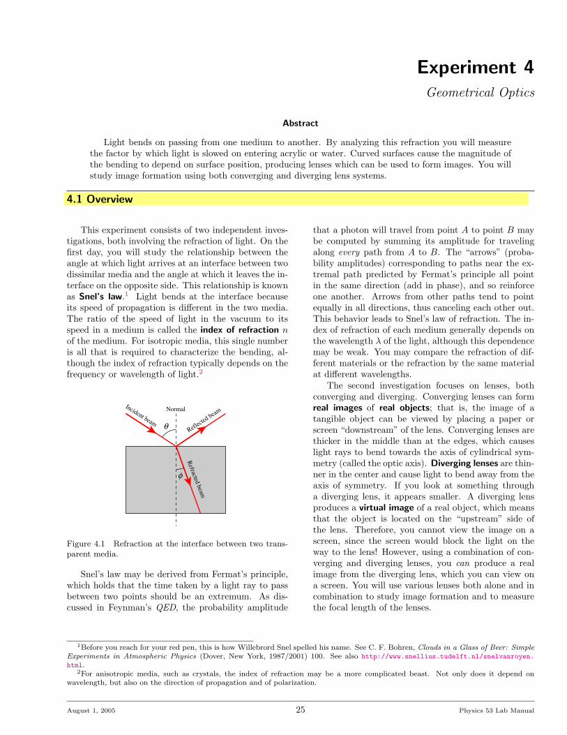
Experiment 4Geometrical Optics

Abstract

Light bends on passing from one medium to another. By analyzing this refraction you will measurethe factor by which light is slowed on entering acrylic or water. Curved surfaces cause the magnitude ofthe bending to depend on surface position, producing lenses which can be used to form images. You willstudy image formation using both converging and diverging lens systems.

4.1 Overview

This experiment consists of two independent inves-tigations, both involving the refraction of light. On thefirst day, you will study the relationship between theangle at which light arrives at an interface between twodissimilar media and the angle at which it leaves the in-terface on the opposite side. This relationship is knownas Snel’s law.1 Light bends at the interface becauseits speed of propagation is different in the two media.The ratio of the speed of light in the vacuum to itsspeed in a medium is called the index of refraction nof the medium. For isotropic media, this single numberis all that is required to characterize the bending, al-though the index of refraction typically depends on thefrequency or wavelength of light.2

θ

φ

NormalIncident beamRefle

cted beam

Refracted beam

Figure 4.1 Refraction at the interface between two trans-parent media.

Snel’s law may be derived from Fermat’s principle,which holds that the time taken by a light ray to passbetween two points should be an extremum. As dis-cussed in Feynman’s QED, the probability amplitude

that a photon will travel from point A to point B maybe computed by summing its amplitude for travelingalong every path from A to B. The “arrows” (proba-bility amplitudes) corresponding to paths near the ex-tremal path predicted by Fermat’s principle all pointin the same direction (add in phase), and so reinforceone another. Arrows from other paths tend to pointequally in all directions, thus canceling each other out.This behavior leads to Snel’s law of refraction. The in-dex of refraction of each medium generally depends onthe wavelength λ of the light, although this dependencemay be weak. You may compare the refraction of dif-ferent materials or the refraction by the same materialat different wavelengths.

The second investigation focuses on lenses, bothconverging and diverging. Converging lenses can formreal images of real objects; that is, the image of atangible object can be viewed by placing a paper orscreen “downstream” of the lens. Converging lenses arethicker in the middle than at the edges, which causeslight rays to bend towards the axis of cylindrical sym-metry (called the optic axis). Diverging lenses are thin-ner in the center and cause light to bend away from theaxis of symmetry. If you look at something througha diverging lens, it appears smaller. A diverging lensproduces a virtual image of a real object, which meansthat the object is located on the “upstream” side ofthe lens. Therefore, you cannot view the image on ascreen, since the screen would block the light on theway to the lens! However, using a combination of con-verging and diverging lenses, you can produce a realimage from the diverging lens, which you can view ona screen. You will use various lenses both alone and incombination to study image formation and to measurethe focal length of the lenses.

1Before you reach for your red pen, this is how Willebrord Snel spelled his name. See C. F. Bohren, Clouds in a Glass of Beer: SimpleExperiments in Atmospheric Physics (Dover, New York, 1987/2001) 100. See also http://www.snellius.tudelft.nl/snelvanroyen.

html.2For anisotropic media, such as crystals, the index of refraction may be a more complicated beast. Not only does it depend on

wavelength, but also on the direction of propagation and of polarization.

August 1, 2005 25 Physics 53 Lab Manual

4.2. BACKGROUND AND THEORY — REFRACTION EXPERIMENT 4. GEOMETRICAL OPTICS

4.2 Background and Theory — Refraction

The angles of incidence θ and refraction φ are il-lustrated in Fig. 4.1, and are related to each other bySnel’s law

n1 sin θ = n2 sinφ (4.1)

where n1 and n2 are the indices of refraction of thetwo media. By definition, the index of refraction is theratio of the speed of light in the vacuum to the speed oflight in the medium. The refractive index of air may betaken equal to one to the accuracy of this experiment.

The law of refraction has an interesting history. Theancient Greeks knew a version of this law that workedonly near normal incidence. Credit for the discoveryof (4.1) is customarily given to the Dutch mathemati-

cian and scientist, Willebrord Snel van Royen (1580–1626), who was the son of a University of Leiden math-ematics professor. He followed in his father’s footstepsat the University of Leiden, focusing his research onmathematics, including trigonometry; cartography; andoptics. He discovered the law of refraction in 1621,3

but did not publish his work. The first published ac-count was given by the French philosopher, mathe-matician, and scientist Rene Descartes (1596–1650) inLa Dioptrique (1637). Descartes did not acknowledgeSnel’s work, although many believe that he had seen it.Notwithstanding this bit of awkwardness, the law of re-fraction is known as Descartes’ law in French-speakingcountries.

4.3 Experimental Procedures — Refraction

In this part of the experiment you are provided witha helium-neon laser of wavelength 632.8 nm, attachedto a circular fixture, the center of which is occupied by asemicircular piece of transparent optical material. Theoptical sample can be rotated so that the entering laserbeam is presented at any desired angle of incidence tothe flat face of the sample (away from the laser). A

measuring tape has been affixed to the circular outsidescreen to permit you to measure the position of the re-flected and refracted laser spots, from which you caninfer the angles θ and φ.

Before beginning to take data, verify the alignmentof the beam through the center point of the samplepiece, and re-check this centering periodically through-

3M. Born and E. Wolf, Principles of Optics, 7th edition (Cambridge, 1999) xxvi.

reflected ray

refractivematerial

normal

measuringscreen

incident ray

He-Ne laser

refracted ray

θ

φθ

Figure 4.2: Index of refraction experimental setup.

Physics 53 Lab Manual 26 August 1, 2005

EXPERIMENT 4. GEOMETRICAL OPTICS 4.3. EXPERIMENTAL PROCEDURES — REFRACTION

Refl Unc Refr Unc

(mm) (mm) (mm) (mm) θ δθ φ δφ n δn

2738.5 1 987 2 0.071 0.003 0.048 0.002 1.463 0.060

2450 1 936 2 0.320 0.003 0.209 0.002 1.513 0.013

2503.5 1 945 2 0.274 0.003 0.179 0.002 1.520 0.016

Figure 4.3: A portion of a spreadsheet to record raw angular position data and to compute angles of reflection andrefraction.

out the session. Think carefully about how you willconvert distance measurements around the circumfer-ence of the measuring screen into the angles of reflec-tion and refraction. As suggested by Fig. 4.2, knowingthe angular position of the zero point and the reflectedand refracted rays allows you to determine the anglesφ and θ. Prepare a spreadsheet to hold the raw posi-tion data, as well as to compute the angles and theiruncertainties. An example is shown in Fig. 4.3.

One convenient way to check the alignment of theincident beam is to look for the faint reflection of thebeam from the curved first surface of the sample; ifthe beam is entering the sample normal to its surface,this reflection will be directed straight back toward thesource.

Warning: Do not look directly into thelaser beam.

Before starting the experiment, describe the beamyou see and give approximate dimensions. Use theseobservations to estimate the uncertainty in your angu-lar measurements.

4.3.1 Measurements

Using the optical acrylic (looks like glass) sample,measure the angles θ and φ at several positions. Makeenough well-spaced measurements that you produce asmooth graph in your spreadsheet and have a good ba-sis for later performing a fit to determine the index ofrefraction, n, of optical acrylic. (If you are efficient, youshould be able to perform that fit while you are still inthe laboratory. As always, ask your professor for helpwith this, if needed.)

Once you have completed these measurements forthe acrylic sample, select one of the following options:

1. Index dependence on material: Replace the sam-ple with the liquid sample container filled withdistilled water, or another liquid provided by theinstructor. This will allow you to contrast therefractive indices of different materials.

2. Index dependence on wavelength: Replace the633-nm (red) He-Ne laser with a 532-nm (green)diode laser. Repeat the measurements on theacrylic sample. This will allow you to observethe phenomenon of dispersion, which is the sub-tle dependence of the refractive index on wave-length. Note: this is a small effect and requiresvery careful measurements!

4.3.2 Analysis

There are two principal ways to analyze your mea-surements. Pick one or the other.

1. Prepare a plot of sinφ vs. sin θ. According to(4.1), you should obtain a straight line with slopeequal to the index of refraction of the semicircu-lar prism (either acrylic or water). Note that ifyou choose this option, you will need to computeδ(sinφ) from δφ via

δ(sinφ) ≈∣∣∣∣d sinφdφ

∣∣∣∣ δφ = | cosφ|δφ (4.2)

This expression is valid only when δφ is measuredin radians.

2. Plot φ vs. θ and fit directly to Snel’s law, (4.1).Use your uncertainties δθ (and δφ) on the plot andtake advantage of a nonlinear fitting program. Inthis case, the program takes care of transformingthe uncertainties for you.

In both cases, note that fitting routines only ac-count for the errors in the dependent variable (plottedon the y axis). If one variable has notably larger uncer-tainties than the other, put that one on the y axis andinvert the fitting function, if necessary. For the cu-rious, see http://www.physics.hmc.edu/analysis/fitting.php#ErrorsOnBoth for a method of account-ing for both x and y uncertainties.

August 1, 2005 27 Physics 53 Lab Manual

4.4. BACKGROUND AND THEORY — LENSES EXPERIMENT 4. GEOMETRICAL OPTICS

4.4 Background and Theory — Lenses

Both the ancient Greeks and Romans knew that acurved glass surface could focus light. Aristophanes’play The Clouds (424 BCE) mentions a “burning glass,”which was used to focus the sun’s rays to produce fire.The behavior of such a convex lens is illustrated inFig. 4.5. The Arabian mathematician Alhazen (965–1038) described how the lens in the human eye formsimages on the retina, and the use of lenses in spectaclesdates from the high Middle Ages in Italy.

The general theory of lenses is quite complicated;lens design is both art and science.4 However, in manycircumstances a simple approximate theory suffices. Weassume that the rays of light make only small angles θwith the optic axis, which is the symmetry axis of thelens(es), so that we may neglect the difference betweensin θ and θ. This is called the paraxial approximation.We also assume that we may neglect the separation ofthe two surfaces of the lens (the thin-lens condition).Under these assumptions, the distance from the centerof the lens to the object (o) and the distance from thecenter of the lens to the image (i) are related by thethin lens equation,

1o

+1i

=1f

(4.3)

where f is the focal length of the lens. These distancesare illustrated for a converging lens in Fig. 4.4.

Image

OpticAxis

f

Figure 4.5 A parallel beam of light converges to a point ata distance f from a convex (converging) lens.

The focal length of a lens depends upon the indexof refraction n of the lens material, and on the radiusof curvature of the two surfaces of the lens, accordingto the lens maker’s formula

1f

= (n− 1)(

1r1− 1r2

)(4.4)

Because the index of refraction depends on the wave-length of light, a singlet lens focuses different colorsslightly differently. You will have an opportunity toobserve this effect by interposing colored glass filtersin the beam from the source and looking for a subtledifference in the focal position of green and red light.

Ray diagrams such as Fig. 4.4 and Fig. 4.7 are ex-tremely helpful in understanding the behavior of lenses,and they are easy to construct. Here are the rules:

(a) A ray that passes through the center of the lensis undeviated.

(b) A ray that propagates parallel to the optic axis(the symmetry axis of the lens) emerges from thelens heading for the image focal point, a distancef downstream of the lens.

4Please note that the singular of lenses is lens, not lense.

Object Image(b)

(a)(c)

ff

o i

(*)

Figure 4.4: Formation of a real image by a converging lens. Light diverges from the object at the left, which is adistance o from the lens. It passes through the lens and converges to form an inverted image a distance i to the rightof the lens. The three principal rays are shown: (a) passes through the center of the lens undeviated; (b) arrives atthe lens parallel to the optic axis and leaves passing through the image focal point, a distance f from the lens; (c)passes through the object focal point on the way to the lens, and emerges from the lens parallel to the optic axis.

Physics 53 Lab Manual 28 August 1, 2005

EXPERIMENT 4. GEOMETRICAL OPTICS 4.4. BACKGROUND AND THEORY — LENSES

(c) A ray that passes through the object focal pointa distance f before the lens emerges from the lensparallel to the optic axis.

The location of the image can be described in twoways. First, if a screen is placed at the location of theimage, a focused picture of the object appears. Second,if you were to look at the system of the object and lensby putting your eye at the location marked with a starat the right of Fig. 4.4, you would see light rays ap-pearing to originate at the location of the image. Thatis, the object would “appear” to be at the location ofthe image. As shown in Fig. 4.4, it would be invertedand it may be either magnified or reduced in size. Youcan readily show from the first principal ray that themagnification is

γ = − io

(4.5)

The negative sign expresses that the image is inverted.

4.4.1 Diverging lens

Diverging lenses are thinner in the center andthicker at the edges; they divert incoming parallel raysaway from the optic axis, as illustrated in Fig. 4.6. Onthe downstream side of the lens the rays appear to di-verge from a point a distance |f | behind the lens, whichis the location of the virtual image. It is virtual, notreal, since you can’t image it by placing a paper orscreen there, the way you can with a real image pro-duced by a converging lens. Because the focus happens

on the upstream side of diverging lenses, their focallengths are negative.

The same set of three principal rays may be drawnfor a diverging lens to locate the virtual image of a realobject, as shown in Fig. 4.7. The trick is to rememberthat the focal points have exchanged places. Therefore,a ray that arrives at the lens parallel to the optic axisemerges from the lens as though it had come from theimage focal point, which is |f | in front of the lens.

OpticAxis

f

VirtualImage

Figure 4.6 Formation of a virtual image from a collimatedbeam by a diverging lens. The image is virtual because itis on the “wrong” side of the lens; you can’t put a screenthere and see it.

Similarly, a ray that is heading towards the objectfocal point a distance |f | beyond the lens emerges fromthe lens parallel to the optic axis.

Just as diverging lenses have negative focal lengths,virtual images have negative image distances i. In thecase illustrated in Fig. 4.7, the image distance i is equalto − 2

3o.

f

Object

Image

(b)

(a)

(c)

f

o

i

Figure 4.7: Formation of a virtual image by a diverging lens. The image is not inverted, is closer to the lens than theobject, and is reduced in size. As in Fig. 4.4, the principal rays are shown: (a) passes through the center of the lensundeviated; (b) arrives at the lens parallel to the optic axis and leaves as though it came from the image focal point,which is |f | from the lens on the upstream side; (c) is heading towards the object focal point, which is a distance |f |downstream of the lens, and emerges from the lens parallel to the optic axis.

Since there are virtual images, could there be vir-tual objects? What would they look like? Well, light di-verges from a real object, as shown at the left of Fig. 4.4.Light also diverges from the real image formed by the

converging lens in that figure. What if you were to stickanother lens downstream of that first image? The rayswould diverge from the first image and propagate to thesecond lens; the image of the first lens serves as the ob-

August 1, 2005 29 Physics 53 Lab Manual

4.5. EXPT. PROC. — IMAGE FORMATION EXPERIMENT 4. GEOMETRICAL OPTICS

ject of the second lens. On the other hand, if you wereto slide that second lens upstream of the real image, asillustrated in Fig. 4.8, the rays would encounter the sec-ond lens before they had finished the job of convergingto produce the first lens’s image (which is the secondlens’s object). Thus, they constitute a virtual objectfor the second lens. Not surprisingly, virtual objectshave a negative object distance o.

AB

C

Figure 4.8 A converging lens forms an image of an objectat A at position B, which is downstream of lens C. Theimage at B is a virtual object for lens C.

Amazingly, the thin lens equation, (4.3), handles allcases for both kinds of lenses, provided you respect thesign conventions outlined above. For easy reference,here’s a table summarizing them:

Qty Positive Negative

f converging lens diverging lenso upstream of lens downstream of lensi downstream of lens upstream of lens

4.5 Experimental Procedure — Image Formation

0 10 20 30 40 50 60 70 80 90 100 110

light source

objectdiv. lensconv. lens

image screen

Figure 4.9: Layout of the optical bench and components.

4.5.1 Preliminaries

Warning: Do not touch the surfaces ofoptical components; handle all optics withcare.

Your lab station should have several converginglenses and at least one diverging lens, mounted in inter-changeable protective holders. The lens mounts allowyou to exchange lenses without having to realign. Selectthe converging lenses and make a quick estimate of theirfocal length by projecting an image of an overhead flu-orescent light on the floor. You’ll probably need to putthe lens closer to the floor than about half a meter tosee an image of the glowing tube. In this case, i o,and if we neglect 1/o compared to 1/i in (4.3), thenthe distance from the lens to the floor is approximatelyequal to the focal length.

Take a look through each lens to get a feel for whatit does to light coming from the opposite side, then se-lect one of the converging lens with a focal length lessthan 25 cm. You will work with it first. Throughoutyour work with the optical bench it is critical for youto record carefully exactly what you are doing. Youwill need to make many sketches, explain tersely howyou made your measurements, and record uncertainties.Since you will be forming images on screens and mea-suring their positions, it will require some judgment onyour part to determine where the position of best focusis. Typically the uncertainty you assign to your mea-surements will be influenced by both your ability toread the bench scale, and by the uncertainty inherentin estimating the position of best focus. Use your sci-entific judgment here and explain the rationale clearlyin your lab notebook.5

5Beware the NFL absurdity: the referee carefully peels off gargantuan bodies as they wrestle for the ball, lovingly extracting thepigskin and setting it gently upon the field somewhere in the vicinity of where it might have been at the end of forward progress (butbefore the post-progress tug-of-war has moved the ball around). The chain gang then trots vigorously out, having carefully marked itslocation with respect to a yard line, and stretches the chain to see whether the nose of the ball has exceeded the requisite 10 yards. Thisfinal measurement is made with great precision as television cameras zoom in for exacting scrutiny. The moral: if you can’t tell betterthan a foot where the lens should go, don’t bother measuring its position to the nearest thousandth of an inch!

Physics 53 Lab Manual 30 August 1, 2005

EXPERIMENT 4. GEOMETRICAL OPTICS 4.5. EXPT. PROC. — IMAGE FORMATION

Sometimes your ability to find the position of bestfocus can be improved by adjusting the brightness of theobject. For example, if the images formed exhibit flar-ing that makes it hard to judge sharpest focus, a pieceof diffusing tissue paper between the illuminator andthe object can dim the images enough to improve theirvisibility. You may also find it helpful and/or interest-ing to insert a colored glass filter to reduce chromaticaberration.

Record raw values first, then compute derived quan-tities. That is, if you are really interested in o, but youmeasure the position xobj of the object and xlens of thelens so you can compute o = xlens − xobj, record bothxobj and xlens in your data table, as well as their differ-ence.

Set up the object and image screens on the opti-cal bench such that an image in sharp focus is formed.Place the object screen at the end of the optical benchnext to the illuminator and adjust it for some conve-nient height. The illuminator should be carefully ad-justed to obtain bright images:

1. Adjust the height of the illuminator to the sameheight as the object and position it at the end ofthe bench.

2. Remove both the white screen and the objectscreen from the bench, and focus the filament ofthe lamp on the far wall (which is effectively at in-finity) by sliding the part that contains the socketin and out.

3. Mount the white screen at the opposite end of thebench and adjust the tilt of the lamp so the beamis centered on the screen, at the same height asthe illuminator.

4.5.2 Converging lens

Now replace the object screen and place the imagescreen at the far end of the optical bench. Place theconverging lens with the shortest focal length betweenthe object and screen, and align the system. Adjustthe position of the lens to produce as clear an image aspossible on the screen. How reproducible is the positionof the lens? That is, if you slide the lens back and thenreposition it to produce the clearest image, how muchvariation in the optimal position of the lens do you getfrom iteration to iteration? Do you and your partneragree? Does the sensitivity depend on where the screenis located?

Pick a particularly good data point and computethe focal length of the lens, as well as its uncertainty.

You may find the following formulas helpful in makinguncertainty calculations:

δ

(1x

)=

∣∣∣∣∂(1/x)∂x

∣∣∣∣ δx =δx

x2(4.6)

δ

(1f

)=

√[δ

(1o

)]2

+[δ

(1i

)]2

δf = f2

√(δi

i2

)2

+(δo

o2

)2

(4.7)

Note that (4.7) assumes that the error in o is uncorre-lated with the error in i, which may or may not be thecase, depending on how you measure.

Repeat this procedure with the other converginglenses.

Even better measurements

Suppose that we plot a series of image and objectdistance measurements in the form of a graph with 1/oon the x-axis and 1/i on the y-axis. Rewriting the lensequation,

1i

=1f− 1o

(4.8)

we see that if the thin lens formula is obeyed, ourgraphed data should describe a straight line with a slopeof −1 and a y-intercept of 1/f , as shown in Fig. 4.10.Notice, as well, that your data points up to this pointall reside in the first quadrant of this plot. Your chal-lenge, now, is to add at least one point in quadrants IIand IV. After you have added these, you will be able tomake a very fine fit for the focal length f of the lens.Note that you will need to use another converging lenssomehow to obtain points in quadrants II and IV. Besure to document your work very carefully. If you arestuck, you might skip to the following section on thediverging lens, and then come back.

1/o

1/i

III

III IV

Figure 4.10 A plot of 1/i vs. 1/o should yield a straightline with slope −1 whose x and y intercepts are 1/f .

August 1, 2005 31 Physics 53 Lab Manual

4.5. EXPT. PROC. — IMAGE FORMATION EXPERIMENT 4. GEOMETRICAL OPTICS

Object(real)

Virtualimageof L1

Realimageof L2

Opticaxis

L1 L2

o1

o2

i2i1d

Figure 4.11: A method for forming a real image from the virtual image of a diverging lens.

4.5.3 Diverging lens

In this part of the experiment, you will investigatethe properties of a diverging lens, again by forming im-ages on a screen, this time using the diverging lens incombination with one or more converging lenses. Apossible geometry is shown in Fig. 4.11. The virtualimage of the diverging lens L1 is located a distance |i1|upstream of the lens, and a distance o2 = |i1| + d up-stream of lens L2.

How could you determine the position of the imageof L1? With both lenses and the screen in place to pro-duce a sharp image of L2, remove L1. The image onthe screen will disappear (or grow diffuse). Now slideforward the object until the image on the screen is onceagain sharp. At this point, the object’s position is thesame as the virtual image of L1 before the lens wasremoved.

4.5.4 Chromatic aberration

If time permits, consider investigating chromaticaberration by forming images with a single converginglens in combination with a colored-glass filter. Becausethe refractive index of glass decreases with increasingwavelength, the focal length of a singlet lens is shorterin the green than in the red. See (4.4). The change infocal length is fairly small—of order 1%—but if you’recareful, you can observe it.

4.5.5 Depth of field

Another possible phenomenon you can investigate isdepth of field. For a camera lens, this is the range ofdistances from the lens that can be imaged (sufficiently)clearly on the film (or sensor) plane. By adjusting theaperture of the lens using an iris diaphragm, which is anadjustable circular opening that limits the effective di-ameter of the lens, the photographer can blur the back-ground (by using a large open aperture) or make every-thing sharp (by using a small aperture). The ratio ofthe focal length f of the lens to the open diameter φ iscalled the “f/number.” A young Ansel Adams foundedGroup f/64 in 1932 as a statement of his æsthetic fa-voring razor-sharp “straight” photography.

A camera lens typically operates at high conjugateratio, which means that the lens is much closer to thefilm plane than to the object being imaged. Select aconverging lens of intermediate focal length and set upan arrangement with the screen near the far end of therail, to allow you a large range of object positions. Forman image with a conjugate ratio of about 4. Mount aniris diaphragm on the object side of the lens and asclose to the lens as possible and investigate how theopen aperture affects the range of object positions thatproduce a well-focused image.

Physics 53 Lab Manual 32 August 1, 2005

Experiment 5Fraunhofer Diffraction

Abstract

Diffraction refers to the fanning out of a wave upon encountering a constriction or obstacle. You willstudy Fraunhofer diffraction from single and multiple slits illuminated with a laser beam. Each point inthe opening serves as a source of secondary waves, whose interference produces the diffraction pattern.Comparing the observed patterns to theoretical curves permits you to make very accurate measurementsof the slit widths and slit separations.

5.1 Overview

As discussed by Feynman in QED, the probabilityfor a photon to pass from the source to the detectormay be calculated by adding up the “arrows” (proba-bility amplitudes) for each path from the source to thedetector, and then taking the square of the resultingarrow (amplitude). For a laser beam normally incidenton one or more slits, the arrows within the slits all pointin the same direction (the amplitudes are in phase withone another), and we may consider this the startingpoint for the interference effects. (The alignment ofthe arrows within the slit is part of the simplificationthat constitutes Fraunhofer diffraction.) For a finite slitwidth, the distance from a point within the slit to thedetector depends upon position within the slit. There-fore, arrows arriving at the detector from different po-sitions within the slit point in different directions andinterfere with one another.

You will investigate how the width of the slit in-fluences the pattern seen far from the slit, as well asthe influence of multiple slits on that pattern. Youshould observe the patterns both qualitatively on apiece of paper and quantitatively using a photodetec-tor, which is mounted behind a narrow window to yielda well-defined diffraction angle. By translating thewindow/detector with a micrometer, and by knowingthe distance between the slit and the window, you canrecord the diffracted intensity as a function of diffrac-tion angle. A computer data logging program will as-sist you in this effort, but you will have to supply thedistances it needs to convert a voltage proportional tomicrometer rotation into a diffraction angle. From thiscalibration, you will then be able to make a very precisedetermination of the slit width (and separation, in thecase of multiple slits).

5.2 Background and Theory

The first mention of diffraction phenomena appearsin the work of Leonardo da Vinci (1452–1519). Over acentury later, a professor of mathematics and physicsfrom Bologna, Francesco Maria Grimaldi (1613–1663),made more careful observations of the phenomenon byilluminating a thin rod by a “pencil” of sunlight ad-mitted into a darkened room. He was surprised to seea shadow behind the rod that exceeded in width thegeometric shadow, and that it was fringed with col-ored bands. Grimaldi coined the term diffraction, whichmeans “breaking up,” to describe the phenomenon andhe developed a theory that light was a fluid that exhib-

ited wave-like motion. His observations were publishedsoon after his death, and this work stimulated IsaacNewton (1642–1727) to study optics.

Newton took up Grimaldi’s observations in the thirdbook of his Opticks (1704). However, Newton’s insis-tence on a corpuscular theory of light prevented himfrom developing a satisfactory theory of diffraction. Acentury later Thomas Young (1773–1829) reported asimpler and more convincing demonstration of “double-slit” diffraction at the 24 November 1803 meeting of theRoyal Society of London, in which he split a narrowpencil of light into two parts using a card held edge-

1See Walter Scheider, The Physics Teacher 24 (1986) 217. Thomas Young’s interests were many and varied; the fact that his con-temporaries weren’t particularly interested in his diffraction experiments was perhaps not terribly troubling to him. He took up otherpursuits. A child prodigy, he was reading fluently at age two and by age 16 was proficient in Greek, Latin, and eight other languages. Heput to good use this facility for languages by helping decipher the Rosetta stone, which had been discovered in 1799 by French troopspreparing the foundation for a fort in the Nile Delta. Young provided the key breakthrough for deciphering ancient Egyptian hieroglyphs:cartouches on the stone contained a phonetic representation of the royal name Ptolemy. Jean-Francois Champollion took up where Youngleft off, applying his linguistic skills and knowledge of Coptic to decipher the rest of the stone. Besides working as a medical doctor,Young also investigated the elastic properties of materials—Young’s modulus relates the stretching of a solid (the strain) to the appliedforce per unit area (the stress).

August 1, 2005 33 Physics 53 Lab Manual

5.2. BACKGROUND AND THEORY EXPERIMENT 5. FRAUNHOFER DIFFRACTION

on into the beam.1 However, British science was un-prepared to admit that the lion, Newton, could haveerred, and further development of the wave theory oflight came on the Continent with the work of FrancoisJean Arago (1786–1853) and especially Augustin Fres-nel (1788–1827). Fresnel produced a mathematical the-ory of diffraction, for which he was awarded the GrandPrix of the French Academy of Sciences in 1819.2

5.2.1 Single slit

To compute the diffraction pattern for a single slit,we must add the amplitudes arising from each pointin the slit. Let x be the position in the slit, whichhas width a, as indicated in Fig. 5.1. If we center ourcoordinates on the slit, −a

2 ≤ x ≤ a2 , then the extra

distance traveled by a wave originating at point x inthe slit, compared to the wave originating at x = 0,is −x sin θ. Its amplitude is therefore proportional toe−ikx sin θ, where k = 2π/λ. We can thus add ampli-tudes (arrows) across the slit with the integral

ψ(θ) ∝∫ a/2

−a/2

e−ixk sin θ dx

=e−ika/2 sin θ − eika/2 sin θ

−ik sin θ

= asin(πa sin θ/λ)πa sin θ/λ

(5.1)

θ

θ

a

x

s

a

Figure 5.1 Geometry of Fraunhofer diffraction. A uniformwave illuminates a slit of width a at normal incidence. Thediffracted light is observed on a screen far from the slit, sothat we may approximate as parallel the rays coming fromeach point in the slit.

Squaring and normalizing, we get the intensity

I(θ) = I0 sinc2

(πa sin θ

λ

)(5.2)

where

sincφ ≡ sinφφ

(5.3)

The single-slit intensity distribution of (5.2) is shownin Fig. 5.2. Of course, when the angle θ is small, it ispossible to approximate sin θ ≈ θ, which simplifies thisexpression somewhat. Is the small-angle approximationappropriate in this experiment?

1.0

0.8

0.6

0.4

0.2

0.0

I / I

o

-3 -2 -1 0 1 2 3

a sinq / l

a

Figure 5.2 Diffracted intensity I(θ)/I0 far from a singleslit, as given by (5.2).

5.2.2 Double slit

It is actually slightly easier to compute the diffrac-tion pattern from a double slit, at least crudely. If wecan neglect the width of the slits, then there are onlytwo “arrows” to sum, giving

ψ(θ) ∝ e−i 12 kd sin θ + ei 1

2 kd sin θ

= 2 cos(πd sin θλ

)(5.4)

where d is the distance between the slits, and we haveused eiφ + e−iφ = 2 cosφ.

However, a more realistic calculation takes into ac-count the finite width a of each slit. We have alreadycomputed the sum of all the arrows from one slit, in(5.1), assuming the slit is centered on the origin. Allwe need to do is slide one slit up d/2 (which multipliesthe integral by e−i 1

2 kd sin θ) and slide the other down d/22There’s a great story about this prize. The prize committee included such notables as Arago, Simeon Poisson, Jean-Baptiste Biot,

and Pierre-Simon Laplace. Poisson, in particular, was sure that Fresnel’s theory was hogwash and set about a calculation of the shadowbehind an opaque disk to see if he could identify a fatal flaw. Indeed, Poisson deduced that along the axis of the disk, where the shadow“should” be darkest, Fresnel’s theory predicted a bright spot, which was obviously absurd. Arago requested that Poisson’s prediction betested, and to the general astonishment of the jury, the spot duly appeared! Fresnel won the prize, but credit for the spot is conventionallyawarded to the skeptical Poisson.

Physics 53 Lab Manual 34 August 1, 2005

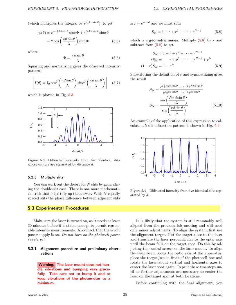
EXPERIMENT 5. FRAUNHOFER DIFFRACTION 5.3. EXPERIMENTAL PROCEDURES

(which multiplies the integral by ei 12 kd sin θ), to get

ψ(θ) ∝ e−i 12 kd sin θ sinc Φ + ei 1

2 kd sin θ sinc Φ

= 2 cos(πd sin θλ

)sinc Φ (5.5)

where

Φ =πa sin θ

λ(5.6)

Squaring and normalizing gives the observed intensitypattern,

I(θ) = I0 cos2(πd sin θλ

)sinc2

(πa sin θ

λ

)(5.7)

which is plotted in Fig. 5.3.

1.2

1.0

0.8

0.6

0.4

0.2

0.0

I / I

o

-6 -4 -2 0 2 4 6

d sinq / l

d

Figure 5.3 Diffracted intensity from two identical slitswhose centers are separated by distance d.

5.2.3 Multiple slits

You can work out the theory forN slits by generaliz-ing the double-slit case. There is one more mathemati-cal trick that helps tidy up the answer. With N equallyspaced slits the phase difference between adjacent slits

is r = e−ikd and we must sum

SN = 1 + r + r2 + · · ·+ rN−1 (5.8)

which is a geometric series. Multiply (5.8) by r andsubtract from (5.8) to get

SN = 1 + r + r2 + · · ·+ rN−1

rSN = r + r2 + · · ·+ rN−1 + rN

(1− r)SN = 1− rN (5.9)

Substituting the definition of r and symmetrizing givesthe result

SN =ei 1

2 Nkd sin θ − e−i 12 Nkd sin θ

ei 12 kd sin θ − e−i 1

2 kd sin θ

SN =sin

(Nπd sin θ

λ

)sin

(πd sin θλ

) (5.10)

An example of the application of this expression to cal-culate a 5-slit diffraction pattern is shown in Fig. 5.4.

1.0

0.8

0.6

0.4

0.2

0.0

I / I

o

-4 -3 -2 -1 0 1 2 3 4

d sinq / l

Figure 5.4 Diffracted intensity from five identical slits sep-arated by d.

5.3 Experimental Procedures

Make sure the laser is turned on, as it needs at least30 minutes before it is stable enough to permit reason-able intensity measurements. Also check that the 5-voltpower supply is on. Do not turn on the photocell powersupply yet.

5.3.1 Alignment procedure and preliminary obser-vations

Warning: The laser mount does not han-dle vibrations and bumping very grace-fully. Take care not to bump it and tokeep vibrations of the photometer to aminimum.

It is likely that the system is still reasonably wellaligned from the previous lab meeting and will needonly minor adjustments. To align the system, first usethe alignment target. Put the target close to the laserand translate the laser perpendicular to the optic axisuntil the beam falls on the target spot. Do this by ad-justing the control screws on the laser mount. To alignthe laser beam along the optic axis of the apparatus,place the target just in front of the photocell box androtate the laser about vertical and horizontal axes tocenter the laser spot again. Repeat these two steps un-til no further adjustments are necessary to center thelaser on the target spot at both locations.

Before continuing with the final alignment, you

August 1, 2005 35 Physics 53 Lab Manual

5.3. EXPERIMENTAL PROCEDURES EXPERIMENT 5. FRAUNHOFER DIFFRACTION

Figure 5.5: Fraunhofer photometer.

should observe a few examples of the single- and double-slit diffraction/interference patterns you will be measur-ing, and determine the effects of varying the slit widthand separation. To do this, remove the photocell mount

at the rear of the photometer box and project the pat-tern on a piece of paper after mounting a slide of singleslits in the holder on the front of the box.

5.3.2 Removing the photocell mount

The photocell mount is secured to the photometerby means of a set screw. The photocell mount is lo-cated at the rear of the light-tight box and the removalof the photocell mount is a simple matter of looseninga set screw and then sliding the photocell mount fromthe backside of the light-tight box. (See Fig. 5.6.)

Figure 5.6 Removing the detector.

The set screw securing the photocell mount to thelight-tight box is accessed via a hole drilled through thetop of the aluminum plate that is attached to the rearof the light-tight box. Move the photocell mount to themidpoint of its travel. Look into the hole in the above-mentioned aluminum plate. You should be able to seethe set screw. Use the hex wrench provided to loosenthe screw.

Warning: Do not remove the set screw.Simply back it out a single turn.

If you’re unable to see the set screw when the photo-cell mount position is set to the midpoint of its travel,

try moving the photocell mount back and forth a shortdistance while looking into the access hole. See yourinstructor for help.

Center the broadest slit in the laser beam. (Note:The clamping screw holding the slide in place should betightened only very lightly by hand. Over-tighteningcan damage the slide.) Sketch the diffraction patternseen when projected onto a piece of paper.

Warning: Do not look directly into thelaser beam!

Try some of the other single slits; then change tothe double slits. From your sketches write down howvarying the distances a and d affect the patterns. Nextremove the slide with the slits from the front of thephotocell box. You should now determine carefully forlater use the distance from the slits on the slide to thephotocell window when it is remounted in its box.

Here are some things to worry about while the pho-tocell is still out:

• How wide is the window (the opening slit mountedin front of the photodiode)?

• How should the window be oriented?

• What is the distance between the target slits andthe window in front of the detector?

When you have sufficiently pondered these questions,replace the photocell in the mounting bracket on theback of the photometer box and tighten the set screwthat holds the photocell in place.

The photocell is positioned by turning a micrometerdrive attached to the back of the photometer box. Themicrometer drive is connected by a gear arrangementto a 10-turn potentiometer. With 5 V applied across

Physics 53 Lab Manual 36 August 1, 2005

EXPERIMENT 5. FRAUNHOFER DIFFRACTION 5.3. EXPERIMENTAL PROCEDURES

the entire potentiometer, the relative position of thephotocell is given by the voltage (0 – 5 V) between thecenter tap and one end of the potentiometer, as read bya voltmeter.

5.3.3 Potentiometer

A potentiometer (as we are using the term) is noth-ing more than a resistor that allows one to make con-nections across the ends of the resistor and between oneend of the resistor and the movable center tap (Fig. 5.7).If 5 volts is set up across the ends of the resistor, thenthe voltage between the center tap and one end of theresistor will vary from 0 to 5 volts linearly with theposition of the tap.

Vout = (Rset/Rmax) Vin

Vin = 5 VRmax

Rset

Figure 5.7 Potentiometer position circuit.

If you haven’t already done so, now would be a goodtime to sketch the experimental apparatus and explainhow it works; i.e., how you can use it to measure adiffraction pattern.

Figure 5.8 The attenuator is the partially silvered glassslide at the left.

For the final alignment, you will use two volt-meters to monitor the photocell position and the photo-

voltage. To avoid saturating the photocell keep V <5 V; you need to reduce the laser beam intensity byadjusting the partially silvered mirror (“beam attenua-tor”) mounted on the rail near the laser (Fig. 5.8). Po-sition the mirror so that the laser beam passes throughit about one-fourth of the way from the top.

Finishing the alignment

Turn on the photocell power. Using the same hexwrench that you used to remove the photocell mount,remove the gear from the end of the potentiometer. Ro-tate the micrometer handle while watching the readingon the voltmeter connected to the photocell output.Adjust the photocell position so that the voltage ob-tained is a maximum. Then adjust the beam attenuatorso that the photocell has an output just less than 5 V soit is not saturated by the laser beam. Next, adjust thepotentiometer until the voltmeter connected across thecenter tap of the potentiometer reads 2.5 volts. With-out rotating either shaft, reinstall the gear onto the endof the potentiometer so that the two gears line up andare flush with each other. This should center the max-imum intensity peak in the range of travel.

At this point you should make fine adjustments ofthe vertical position of the laser beam spot by adjust-ing the tipping screw on the laser’s seesaw bracket. Ad-just for maximum photo-voltage. Now, again adjust thebeam attenuator to give a non-saturating peak photo-voltage close to, but not exceeding, 5.0 V.

Change the micrometer position and note the in-tensity profile of the laser beam. If you did everythingcorrectly, you should see a steep but smoothly varyingprofile with a peak photo-voltage of a bit less than 5.0 Vat a micrometer position voltage near 2.5 V.

5.3.4 Beam profile

You will be using a computer program to aid youin taking data and in comparing your results with thetheoretical expressions of section 5.2. The voltages fromthe potentiometer and photodetector are converted todigital values by an analog-to-digital converter (ADC),which is connected to a USB port on the computer.During an acquisition, these voltages are sampled sev-eral times per second and plotted in real time as photo-voltage vs. position voltage, allowing you to monitorthe data as you slowly rotate the micrometer or poten-tiometer gear to translate the detector window.

To get a feel for how the acquisition program works,you should first take a scan of the laser beam itself, withno target slit mounted at the front of the photometerbox. If Igor is not already running, launch the program

3 Igor is a powerful data acquisition, analysis, and graphics program that runs on both Macintosh and Windows. Unlike Kaleidagraph,Igor is entirely scriptable: virtually everything that can be accomplished using the graphical user interface can be programmed within Igorusing a C-like programming language. The programs that acquire and analyze data for the RLC and Fraunhofer diffraction experimentsproduce Igor experiment files holding your data, graphs, and tables, as well as a history of the operations you conduct. You may usethem to export data in text format for further analysis in Kaleidagraph, Origin, or other program, or you may analyze your data further

August 1, 2005 37 Physics 53 Lab Manual

5.3. EXPERIMENTAL PROCEDURES EXPERIMENT 5. FRAUNHOFER DIFFRACTION

by clicking on the Igor icon in the Dock at the rightof the screen. It is shown in Fig. 5.9. Then select theFraunhofer Diffraction program.3

Figure 5.9 Igor icon.

Rotate the micrometer to one edge of its range, notethe position of the micrometer (see Fig. 5.10), then clickthe Take Data button.

Warning: There is a long delay (up to 20

seconds) the first time you take data, asthe National Instruments driver softwareis loaded into memory. Be patient and donot touch the computer during this pe-riod.

Smoothly turn the micrometer shaft or gear to ad-vance the detector. Watch the computer screen as yougo to make sure that the data are smooth and quiet. Donot reverse the direction of the photocell motion whilecollecting data. If you do, you will see the effects of“screw backlash” in your data. Scan through the com-plete 5-V range of the potentiometer, then hold downthe Shift key to finish the acquisition. Note that thevertical axis rescales automatically during the acqui-sition, so that the noise in early points may appearexaggerated.

Figure 5.10 Reading the micrometer: it takes four revolu-tions to advance by one “major” unit. What do you supposethose units are? How could you check?

You may save and print these data, if you wish, butyou should at least note the width of the beam, whichyou can readily convert from volts to distance. De-termine the distance the micrometer has advanced and

use this information to calculate the width of the laserbeam. Is your value reasonable?

5.3.5 Taking data

At this point you are ready to take diffraction data.Select the slide of single slits and note the labeling ofthe slide and the slits (it will be handy later to haveidentified each slit before installing the slide). Placethe slide in the holder at the front of the photocell boxand center the slit you have selected under the laserspot. Advance the micrometer until the potentiometervoltage is about 2.5 V, and scan a short ways in ei-ther direction to look for the maximum intensity. Atthe maximum, adjust the attenuator slide to producea peak intensity slightly lower than 5 V. Then set themicrometer at the edge of its travel.

Start the data acquisition and carefully scan the mi-crometer across the full range of its motion, watchingthe computer screen to monitor the data acquisition asyou go. You should also confirm that the program isin agreement with the voltage levels reported on themultimeters. Hold down the Shift key when you havefinished.

When you are satisfied with your data, click theNormalize tab. To convert your position data (in volts)to angles, you must enter the complete angular range ofmotion of the detector window (corresponding to a 5-Vchange in the potentiometer voltage). Make a sketchof the relevant geometry in your notebook, and use thedistance from the target slit to the detector windowto compute the full angular range, in radians. Enterthis value in the box, then click the Normalize button.The Normalize routine both scales and shifts the datato produce a maximum peak height of 1 centered atθ = 0. For best results you should make sure to gosmoothly and rather slowly over the central maximumso the program can make an accurate determination ofthe peak height and position.

Comparing to theory

To compare your data to (5.2), click the Slit Dimen-sions tab and enter the slit width. Best estimates ofthe various slit widths and separations are provided ona sheet near the photometer set-up. Then select 1 slitfrom the popup menu. You should see the computedcurve superimposed on your data, as well as a panelof residuals at the top of the graph. The residual of adata point is its vertical distance from the computedcurve. When a curve accurately describes experimen-tal data, the residuals should be randomly distributedwith respect to the zero line. When there are signifi-cant disagreements between the curve and the data, theresiduals will exhibit a pattern.

If the calculated curve is either fatter or skinnierthan the central peak in your data, click on the Hypo-

within Igor. See http://www.physics.hmc.edu/analysis/Igor.php for further information about using Igor.

Physics 53 Lab Manual 38 August 1, 2005

EXPERIMENT 5. FRAUNHOFER DIFFRACTION 5.3. EXPERIMENTAL PROCEDURES

thetical Dimensions tab and enter a different value forthe slit width, adjusting that value until you get thebest agreement. Note that when a hypothetical curveis plotted, the residuals panel is adjusted to show resid-uals for the hypothetical curve. To narrow the peak doyou have to increase or decrease the value of the slitwidth? Why?

If you find that you must vary the hypothetical slitwidth appreciably from the expected value, stop andtake stock of your procedure. The slit widths were mea-sured carefully with a high-quality optical microscope.Is it likely that the sheet of slit widths is significantlyoff? What else could account for the discrepancy? Jotsome ideas in your notebook as you try to work thatout the problem.

Saving and printing

When you have found the best value for the hy-pothetical slit width, save and print your data. Clickthe Save & Print tab and click the Save button. Youwill be asked for each partner’s name and your sectionnumber so your data can be stored in your own localdirectory (you will be able to copy the files to yourown computer or your Charlie account later). A dia-log will tell you the name of the data file, which youshould record in your lab notebook. This informationis also copied to the History window at the bottom ofthe screen.

Then click Print. You will be asked for a (brief)comment. You may leave this blank, or enter a shortdescription (e.g., “Marge Inovera turned the microme-ter”). After this dialog is closed, you will be pesteredwith one more to check the positioning of the graph an-notations. Sometimes the text will overlap your data.Using the mouse, drag any annotations that are poorlypositioned into appropriate places, then click the Printbutton.

Two copies of the graph will be printed, one foreach partner. Cut the page in half, tape the graphinto your lab notebook, and comment briefly on the ex-tent of agreement between your data and the calculatedcurve(s) on the same notebook page. To test repeata-bility, you should realign the apparatus and record asecond run.

Explore

At this point you should be up and running withthe acquisition program.

If all has gone well in the first week, you should bewell into computer data taking by your second lab pe-riod. Repeat the experiment using another single slit,two different double slits and the three-, four-, and five-slit configurations. Readjust the laser optics to elimi-nate any saturation of the photocell response at inten-sity maxima and for a maximum as large as possiblebut not to exceed 5 V. Carefully re-center each set of

slits in the laser spot. There is a second set of gearsyou can use to change the range of the photocell posi-tions. These gears should be used for some of the slitsto record a useful portion of the pattern. Note thatyou will need to recompute the total angular rangefor the new gear set.

In analyzing your results, there are a number ofopportunities for quantitative comparison with theory.Your experimental curves should have the correct gen-eral qualitative form, but they will unavoidably differfrom the ideal theory in some particulars. The posi-tions (and uncertainties!) of the experimentally ob-served maxima and minima should be used togetherwith different trials for the hypothetical parameters toderive refined estimates of the slit dimensions and theiruncertainties for one particular single slit and one par-ticular pair of double slits. (These can be comparedwith direct microscopic measurements.)

Discrepancies in the heights, depths and symmetriesof the peaks should give you food for thought and fur-ther analysis. The theory section makes certain simpli-fying assumptions about the illumination and geome-try that may not describe your experiment accurately.Many of these “non-idealities” can be profitably simu-lated and studied at length in the context of a labora-tory report. Finally, you should use the trends of yourplots for the 3, 4, and 5 slit patterns to describe theeffect of increasing the number of slits, and explain thecause of this effect.

5.3.6 Program details

The program has two adjustable parameters to tai-lor the acquisition to your needs: the number of in-dividual analog-to-digital values to average to produceeach data point, and the number of data points per sec-ond to record. While you are acquiring data, the dataacquisition board samples the two input channels at asteady rate of 104 samples per second on each channel.To reduce electronic and digitization noise, many sam-ples are averaged together to produce each data point,and their standard error is recorded as the uncertaintyof the data point.

You may set the number of samples to average foreach data point. The default value is 100, which meansthat each data point is acquired during a time of 10 ms.You may also set the number of data points you wishrecorded each second. Note that this value is only ap-proximate. The default value is 5, but you may wish tosample either more or less rapidly.

Note that when you normalize your data, the un-certainties are scaled by the same factor as the data, sothat their relative value remains unchanged.

5.3.7 Saved data

The program saves your data in two different places.First, it is copied into a data folder within the Igor

August 1, 2005 39 Physics 53 Lab Manual

5.3. EXPERIMENTAL PROCEDURES EXPERIMENT 5. FRAUNHOFER DIFFRACTION

experiment itself. Second, it is exported to a tab-delimited text file in a subfolder of the Data folder onthe Desktop of the computer. Open this folder, thenopen your section’s folder, and then open the foldernamed for you and your partner. Each file is namedFraun xxxx, where xxxx represents the time at whichthe data were saved.

The text file format is tab-delimited text, which canbe opened by any data analysis package. The first rowholds column labels, and subsequent rows hold the data.There is a potential gotcha with text files: differentoperating systems use different characters to indicatethe end of a line. UNIX computers use the linefeed

character (LF = ASCII 10), Macintosh computers usethe carriage return character (CR = ASCII 13), andDOS/Windows computers use both (CR+LF)! If yourdata analysis program has trouble reading the file, youcan use Excel to open it first and handle the conversionof line terminators.

To copy the data to your Charlie account, make sureyou are in the Finder (check the first text item in themenubar at the top of the screen; if it isn’t Finder, thenclick the first icon in the Dock) and press Command-K or select Connect to Server. . . from the Go menu.Enter charlie.ac.hmc.edu and you will be presented alogin dialog.

Physics 53 Lab Manual 40 August 1, 2005

Experiment 6The Grating Spectrometer and the Balmer Series

Abstract

The colors emitted by many sources of light provide a spectral fingerprint that uniquely identifies them.You will study the discrete line spectrum of two elements having a single electron in their outermost shell:sodium and hydrogen. Using literature values for the wavelengths of the yellow sodium doublet, you willcalibrate the period of a diffraction grating. You will then measure the wavelengths of four visiblehydrogen lines and compare them to the Balmer equation, deducing a value for the Rydberg constant.

6.1 Overview

A diffraction grating is a transparent or opaque sub-strate on which a series of fine parallel, equally spacedgrooves are patterned. When a light wave illuminatesa grating, each groove scatters light in all directions.However, the scattering will be appreciable only in di-rections for which the light from adjacent grooves ar-rives in phase. The behavior of diffraction gratings canthus be readily explained using the wave theory of light.

Diffraction gratings may be used to disperse the col-ors of a polychromatic source and to identify its compo-nent wavelengths. To make a quantitative identificationof the wavelengths, you will need to calibrate the grat-ing, which means to determine the distance d betweenrulings. The grating you will use has a nominal pe-riod1 of 600 lines/mm, but you will determine d muchmore accurately than the 1 significant figure impliedby this value by observing the yellow light of a sodiumlamp. You have probably seen the bright yellow lightof a sodium lamp in parking lots, where they are usedbecause of their energy efficiency and power. By takingas given the literature values for the wavelengths of thetwo adjacent sodium lines,2 and by measuring preciselythe angles at which the yellow light is diffracted by thegrating, you can determine d.

Having calibrated the grating, you will then studythe spectrum of a Balmer hydrogen discharge tube,which allows you to investigate the energy levels of ahydrogen atom. When an atom in an excited electronicstate relaxes to a lower-energy state, it emits the energydifference between the states in the form of a photon oflight. In the case of hydrogen, most of these transi-tions produce photons either in the ultraviolet or theinfrared. For four transitions ending in the n = 2 level,the emitted photons are visible and you can study themby eye using the grating you have calibrated with thesodium lines.

Figure 6.1 The line spectrum of hydrogen.

6.2 Theory

In 1666 while Isaac Newton (1642–1727) was homein Lincolnshire because the plague had closed Cam-bridge University down, he discovered that whereas asingle prism of glass would cause sunlight to fan outinto a rainbow of colors, a subsequent prism caused no

further color changes. Newton reasoned that sunlightwas a mixture of all colors, and that a prism caused thevarious colors to bend (or refract) differently, therebyproducing a smooth, continuous band of gradually vary-ing appearance.

1“Nominal” here means “named”; that is, the manufacturer’s stated value.2The discrete wavelengths at which a particular atom or molecule emits light are called “lines” because this is how they appeared on

photographic plates in the early days of spectroscopy (see Fig. 6.1). A diffraction grating fans the light out in one direction, but doesn’taffect the extent of the beam in the perpendicular direction. Hence, the “signal” on the photographic plate looks like a line segment.

41

6.2. THEORY EXPERIMENT 6. GRATING SPECTROMETER

A century and a half later in 1814, an orphanedglassmaker, Joseph von Fraunhofer (1787–1826), dis-covered that the smooth solar spectrum was actually in-terrupted by a series of dark lines.3 To study these darklines quantitatively, Fraunhofer invented the diffractiongrating.4 By mid-century, scientists had determinedthat the dark (absorption) lines and the identically lo-cated bright (emission) lines serve as spectral finger-prints, uniquely identifying the atomic species involved.Comparing the yellow light of sodium to a prominentdark line in the solar spectrum allowed Gustav Kirch-hoff (1824–1887) and Robert Bunsen (1811-1899) to de-duce the presence of sodium in the solar atmosphere.

The positions of the spectral lines of different sub-stances made a challenging puzzle to nineteenth centuryscientists—and to modern quantum theory, for all butthe simplest atoms! In 1885, J. J. Balmer (1825–1898)showed that the wavelengths of the visible spectral linesof hydrogen were given by the expression

1λ

= R

(1N2

− 1n2

)(6.1)

where n is an integer and N = 2 for the visible linesof the Balmer series. The hunt was on to find a theorythat could explain Balmer’s relationship.

At the end of the century, Max Planck (1858–1947)found he could explain the smooth (dominant) part ofthe solar spectrum with the help of the relation

∆E = hν =hc

λ(6.2)

between the frequency and the quantum of energy emit-ted or absorbed by an atom. Niels Bohr (1885–1962)combined the Planck relation with his own idea of angu-lar momentum quantization to produce a simple theoryfor the hydrogen atom that reproduced Balmer’s rela-tion, (6.1). Bohr’s model described unphysical micro-scopic solar systems, but the principal idea of angularmomentum quantization survived the birth of modernquantum mechanics in 1925–26 and the hydrogen atomcalculations of Heisenberg (1901–1976) and Schrodinger(1887–1961).

Figure 6.2 A schematic representation of quantized atomicenergy levels.

Quantum mechanics also tells us that electrons inorbit around a nucleus cannot have just any energy(like planets orbiting the Sun), but are restricted tocertain quantized energy levels (Fig. 6.2). This pre-diction of quantum mechanics explained the previouslymysterious fact that elements emitted light only at dis-crete wavelengths. Quantum mechanics was able toexplain and quantitatively predict the wavelengths ofthese spectral lines for hydrogen, the simplest element.This confirmed the relation that had been empiricallydiscovered by Balmer for the wavelength of the visiblehydrogen lines,

In (6.1), N and n are integers corresponding tothe lower and upper energy levels, respectively. Forthe visible Balmer series, the lower level always cor-responds to N = 2. However, n is different for eachspectral line in the series, each corresponding to a dif-ferent upper energy level. The constant R is known asthe Rydberg constant, with an accepted value (1998) ofR = 1.097 373 157 × 107 m−1. In this experiment youwill first observe and carefully measure the wavelengthsof these spectral lines, and then determine best valuesfor n and R.

The technique used in this experiment to mea-sure the wavelengths makes use of diffraction gratings.When parallel light is incident upon an array of manyequally spaced rulings on a transparent substrate, lightemerges on the other side at certain specific angleswhere constructive interference occurs among the simul-taneously illuminated rulings. These intensity maximaoccur at angles θ for which

d sin θ = mλ m = 0,±1,±2, . . . (6.3)3Fraunhofer’s childhood augured anything but a scientific career. Orphaned at age 11, he was not strong enough to become a wood

turner and was apprenticed to a glassmaker, Philipp Anton Weichselberger. Weichselberger did his level best to frustrate the intellectualcuriosity of the boy for the next two years, but Fraunhofer’s life took a sudden turn when Weichselberger’s house/workshop collapsedin 1801. After being buried in the rubble for several hours, Fraunhofer was rescued and came to the attention of Prince Elector MaxIV Joseph, who directed the rescue operation. The prince took an interest in Fraunhofer and made sure that he had books and time tostudy while he learned the craft of lens grinding.

At age 22 he was appointed head of the glass factory in Benediktbeuern, where he worked to develop new types of glass and on methodsto avoid streaking and inhomogeneities. He expanded the product line to include telescopes, binoculars, microscopes, magnifying glasses,and the best and largest telescopes at the time. He invented the spectroscope in 1814 and the diffraction grating in 1821.

4Evidently, the American D. Rittenhouse preceded Fraunhofer by 28 years, but his work was hardly noticed. See M. Born and E.Wolf, Principles of Optics, 7th Edition, Cambridge, 1999, p. 453.

Physics 53 Lab Manual 42 August 1, 2005

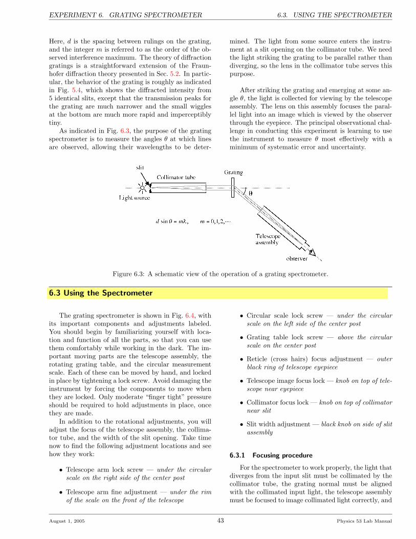
EXPERIMENT 6. GRATING SPECTROMETER 6.3. USING THE SPECTROMETER

Here, d is the spacing between rulings on the grating,and the integer m is referred to as the order of the ob-served interference maximum. The theory of diffractiongratings is a straightforward extension of the Fraun-hofer diffraction theory presented in Sec. 5.2. In partic-ular, the behavior of the grating is roughly as indicatedin Fig. 5.4, which shows the diffracted intensity from5 identical slits, except that the transmission peaks forthe grating are much narrower and the small wigglesat the bottom are much more rapid and imperceptiblytiny.

As indicated in Fig. 6.3, the purpose of the gratingspectrometer is to measure the angles θ at which linesare observed, allowing their wavelengths to be deter-

mined. The light from some source enters the instru-ment at a slit opening on the collimator tube. We needthe light striking the grating to be parallel rather thandiverging, so the lens in the collimator tube serves thispurpose.

After striking the grating and emerging at some an-gle θ, the light is collected for viewing by the telescopeassembly. The lens on this assembly focuses the paral-lel light into an image which is viewed by the observerthrough the eyepiece. The principal observational chal-lenge in conducting this experiment is learning to usethe instrument to measure θ most effectively with aminimum of systematic error and uncertainty.

Figure 6.3: A schematic view of the operation of a grating spectrometer.

6.3 Using the Spectrometer

The grating spectrometer is shown in Fig. 6.4, withits important components and adjustments labeled.You should begin by familiarizing yourself with loca-tion and function of all the parts, so that you can usethem comfortably while working in the dark. The im-portant moving parts are the telescope assembly, therotating grating table, and the circular measurementscale. Each of these can be moved by hand, and lockedin place by tightening a lock screw. Avoid damaging theinstrument by forcing the components to move whenthey are locked. Only moderate “finger tight” pressureshould be required to hold adjustments in place, oncethey are made.

In addition to the rotational adjustments, you willadjust the focus of the telescope assembly, the collima-tor tube, and the width of the slit opening. Take timenow to find the following adjustment locations and seehow they work:

• Telescope arm lock screw — under the circularscale on the right side of the center post

• Telescope arm fine adjustment — under the rimof the scale on the front of the telescope

• Circular scale lock screw — under the circularscale on the left side of the center post

• Grating table lock screw — above the circularscale on the center post

• Reticle (cross hairs) focus adjustment — outerblack ring of telescope eyepiece

• Telescope image focus lock — knob on top of tele-scope near eyepiece

• Collimator focus lock — knob on top of collimatornear slit

• Slit width adjustment — black knob on side of slitassembly

6.3.1 Focusing procedure

For the spectrometer to work properly, the light thatdiverges from the input slit must be collimated by thecollimator tube, the grating normal must be alignedwith the collimated input light, the telescope assemblymust be focused to image collimated light correctly, and

August 1, 2005 43 Physics 53 Lab Manual

6.3. USING THE SPECTROMETER EXPERIMENT 6. GRATING SPECTROMETER

eyepiece

diffractiongrating

collimatortube

slitassembly

telescopeassembly

autocollimationmirror

lightsource

illuminationpower supply

measurementscale

Figure 6.4: Photo of grating spectrometer and supporting equipment.

it must respect the grating axis. The following proce-dure will allow you to achieve these conditions.

Warning: Never touch a grating! Grat-ings cannot be cleaned, and are signifi-cantly degraded by fingerprints and dirt.

1. First you must adjust the telescope assembly toimage collimated (parallel) light properly. Lookthrough the eyepiece and rotate the ocular untilthe black crosshairs are clear and sharp.

2. Turn on the illumination power supply and placethe autocollimation mirror on the grating table,aimed to reflect light back into the telescope. Ro-tate the mirror slowly while looking through theocular until you see a green cross. Light from thegreen cross reflects from a mirror inside the eye-piece assembly, is collimated by the telescope lens,bounces off the autocollimation mirror, and thenback down the telescope to be viewed through theeyepiece.

When the green light is collimated at the mirror,the green cross will appear sharp and clear. Bysliding the eyepiece in its sleeve, adjust the focusof the green cross until it is sharpest. Lock theeyepiece in place, keeping the reticle line paral-lel to the slit image. You should now see boththe black crosshairs and the green cross sharplyfocused.

3. At this point it would be helpful to make surethat both partners can see both the green crossand the crosshairs simultaneously in focus. Ei-ther partner is allowed to adjust the ocular only.This accommodates for differences between eye-balls; no other adjustment should be necessary.If it is, go back to the previous step.

4. You must now make sure that the normal to thegrating is aligned with the axis of the telescope(which is fixed). Remove the autocollimation mir-ror and rotate the grating table so that the grat-ing can reflect (like a mirror) the green cross lightback down the telescope. Locate the brightest im-age of the green cross, rotate the grating to centerthe image in the eyepiece, and adjust the tilt ofthe grating table to put the strongest green crossat the horizontal crosshair in the top half of thefield of view. [Since the source of the green crossis at the bottom of the field of view, its imageshould appear symmetrically in the top part.]

5. Looking through the telescope eyepiece, line upthe telescope and collimator tube so that the slitimage is centered, vertical, and focused. You mayslide the slit assembly in or out of the tube slightlyto achieve best focus. Then lock it in place.

6. With the slit image carefully centered in the reti-cle adjust the circular scale until it is zeroed, andlock it in place.

Physics 53 Lab Manual 44 August 1, 2005

EXPERIMENT 6. GRATING SPECTROMETER 6.4. EXPERIMENTAL MEASUREMENTS

7. Rotate the grating table so that the ruled faceof the grating faces the telescope and make surethat the grating is centered in the holder. Lock

the grating table to prevent further rotation, andturn off the green illumination source.

6.4 Experimental Measurements

6.4.1 Grating calibration

From (6.3), it is evident that the observed positionθ of a spectral line allows its wavelength λ to be de-termined provided that the grating spacing d is known.The grating in this experiment is known to have a nom-inal spacing of about 600 lines/mm, but a more precisedetermination of d is required. For this purpose, wewill take the wavelengths of the yellow sodium doublet(588.995 nm and 589.592 nm) as accepted standards.

Turn on the sodium vapor lamp and place it at theslit opening of the spectrometer. It will take severalminutes for the light to change from a pinkish mixtureof contaminant wavelengths to the pure yellow colorcharacteristic of Na. While it is warming up, rotate thetelescope arm of the spectrometer and look for a seriesof red lines, as well as the yellow lines of the sodiumdoublet. [Until you have calibrated the grating, you arenot in a position to measure the wavelength of some ofthe red lines; however, an investigation of these linesto determine the contamination gas could be an inter-esting topic for a technical report.] Using the nominalvalue for d, estimate the angle(s) at which you expectto find the sodium doublet, and use the spectrometerto look for them.

During this step, you’ll be learning how to use thespectrometer, which will help you find the more diffi-cult lines of the hydrogen spectrum. One of the ad-justments available to you is the slit width. The widerthe slit opening, the brighter is the light seen, whichmay be helpful in trying to view particularly faint lines.(You can also see fainter lines more easily by darkeningthe room, using a black cloth to shield outside light,and allowing 10 minutes or so for your eyes to becomedark adapted.) A wider slit opening however, has theundesirable effect of making the line image wider, andtherefore making the uncertainty of its position greater.You’ll note that if you make the slit wide enough, theimages of the two doublet lines will merge together intoone wide line.

Make adjustments until you achieve a good compro-mise between maximum sharpness and adequate visibil-ity. Now is a good time to make and record estimatesof the uncertainties in θ and λ associated with yourchoice(s) of slit width. Also note that in addition tothe uncertainty caused by finite slit width, the spec-tral lines will have a finite width due to the resolvingpower of the grating. The smallest resolved wavelengthdifference ∆λ is

λ

∆λ= Nm (6.4)

where m is the order and N is the number of gratingrulings illuminated. If you use a piece of paper to coverpart of the width of the grating, you should see the ap-parent line width increase accordingly. Using standarderror propagation, this effect should be incorporatedinto your uncertainty budget.

(A) (B)

Figure 6.5 The vernier allows you to read angles to thenearest minute of arc. Start at (A) to determine 336 <θ < 33630′. Then look for the lines that match up best at(B) to obtain the final value 33620′.

Make careful measurements of θ for both the sodiumdoublet lines on both sides of zero, for as many ordersas you can. Figure 6.5 shows how to read the vernier toabout 1 minute of arc. At this point you may wish tothank the ancient Sumerians for the sexagesimal sys-tem we use for telling time and measuring angles. Ifyou have been careful in the alignment of the spectrom-eter and grating, the right and left angles of deflectionshould agree with one another to better than 10′; ifthey do not, now is the time to tweak the grating posi-tion to get symmetric readings, in preparation for thehydrogen measurements.

From your Na measurements, determine the bestvalue for d to be used in the study of the hydrogenspectrum in the next part. You will probably note thatsome orders appear brighter than others, and that thelines may appear brighter or clearer on one side thanthe other. This is because the grating is blazed or op-timized for maximum output in a particular direction.Make note of this information, as some of the fainterhydrogen lines may be hard to observe in any but thebrightest and best conditions. Consider carefully theuncertainty of your data in deciding whether to use the

August 1, 2005 45 Physics 53 Lab Manual

6.5. EXPERIMENTAL ANALYSIS EXPERIMENT 6. GRATING SPECTROMETER

first- and/or second-order measurements in obtaining acalibration for d and also in determining the hydrogenwavelengths.

6.4.2 Hydrogen observations

Replace the Na lamp with the Balmer hydrogen dis-charge tube lamp.

Warning: Be sure to turn on the coolingfan and direct it toward the base of theBalmer tube, or overheating may result.

Observe the hydrogen spectrum. You will be look-ing for four visible wavelength lines, corresponding tocolors of deep violet, violet, blue-green, and red. (Theshortest wavelength line can be particularly hard to see,and may require some patience and observation skill tolocate and measure.)

Record the color and angular position of all the spec-tral lines in all of the orders in which they can be ade-quately observed. Include appropriate uncertainties foreach measurement, so that the correct relative weight-ing can be assigned to observations of differing qualityin coming up with a final set of “best results” for thehydrogen wavelengths. Calculate the final values andpropagated uncertainties for the wavelengths of the hy-drogen Balmer lines.

6.4.3 Forensic investigation

If time permits, return to the sodium lamp, whichshould now be cool again, and investigate the pink lightit gives off before the discharge warms up. At room tem-perature, the vapor pressure of sodium in the lamp istoo small to operate the electric discharge. Therefore,the lamp is filled with buffer gas to help the lamp get go-ing. For the sodium lamp to work efficiently, the sodiumvapor must be heated by the discharge to 260C. Dif-ferent buffer gases may be used in sodium lamps to helplaunch the discharge and heat the sodium. Such gases

must not react with sodium metal, or sodium vaporwould be chemically removed from the cell.

You can figure out what is in the lamp if you usethe spectral finger print of the buffer gas(es). Record asprecisely as you can the positions of several prominantspectral lines, and convert them to wavelengths. Youcan then look them up at http://cfa-www.harvard.edu/amdata/ampdata/kurucz23/sekur.html.

To use the web-based database, you must enterranges for several parameters. Here’s how to find thesodium lines you have already observed:

1. Set the range from 500 nm to 700 nm.

2. Set the oscillator strength range from −2 to 4.Bright lines have large oscillator strength.

3. Set the lower level range from 0 to 105 cm−1 andthe upper level range from 0 to 4× 105 cm−1.

4. Select all the Na items in the left column, thenclick Search.

You should see a listing of 8 spectral lines, includ-ing the two prominent lines of the sodium doublet. No-tice that these are the only entries in this wavelengthrange that have the ground state as the lower energylevel. Notice further that these lines are described byNa I, which is traditional spectroscopic notation for theneutral sodium atom. (Na II indicates singly ionizedsodium, Na III is doubly ionized, etc.)

Another useful web site for spectral lines ismaintained by the National Institute for Standardsand Technology (NIST). It is available at http://physics.nist.gov/PhysRefData/Handbook/Tables/findinglist.htm. At this page, the lines are sorted bywavelength in 100-nm bands. However, you can clickon the Element Name button to select a particularelement, from which you can then display the strongestspectral lines, or focus only on the lines of the neutralatom.

6.5 Experimental Analysis

One simple way to evaluate your results is to com-pare them with accepted literature values, shown in thetable below. Statistically characterizing any discrepan-cies as random or systematic, probable or improbable,is important to demonstrating your understanding ofthe experiment.

Color Wavelength

red 656.17 nmblue-green 486.13 nm

violet 434.05 nmdeep violet 410.17 nm

A somewhat more instructive analysis is obtainedby comparing your results with the predictions of theBalmer relation of (6.1). There are a couple of ways tomanage this. Pick either one.

• A plot of 1/λ as a function of 1/n2 should the-oretically yield a straight line, whose slope andy-intercept are related to the Rydberg constantand the value for the constant N . (Here, the con-secutive integers n index the energy levels cor-responding to each line; it will be up to you todetermine convincingly what they are for the ob-served lines by comparing the linearity of the fit ofthe Balmer formula for several plausible choices of

Physics 53 Lab Manual 46 August 1, 2005

EXPERIMENT 6. GRATING SPECTROMETER 6.5. EXPERIMENTAL ANALYSIS

the sequence of n values.) You should prepare theplot giving the best straight line fit, along withappropriate error bars and a properly weightedlinear fit determining R and N .

• Plot λ vs. n and fit to (6.1). You don’t neces-sarily know the values of n, although you mayassume that you have measured lines correspond-ing to consecutive integers. Therefore, you mayfit to a modified version of (6.1):

λ(n) = R−1

(14− 1

(n+ n′)2

)(6.5)

where n′ is a fitting parameter that should comeout very nearly equal to an integer.

As before, discuss the results and their agreement(or lack thereof) with theoretical and accepted values.(How does your value of the Rydberg constant constrainother fundamental physical constants?) As quantita-tively as possible, ascribe any discrepancies to sourcesof uncertainty in the experimental equipment and pro-cedures. For example, if there is a lingering systematicbias between your wavelength estimates from the rightand left sides, you should quantitatively investigate theorigin of this error, and attempt to correct for it in com-ing up with your final results. Although the results ofthis experiment are actually well known to the physicsworld, you should approach the analysis task as if theresults are original, and strive to be as precise and rig-orous as possible in obtaining them.

August 1, 2005 47 Physics 53 Lab Manual

Part III

Appendices

48

Appendix AElectric Shock – it’s the Current that Kills

Naively, it would seem that a shock of 10 kV wouldbe more deadly than 100 V. This is not necessarilyso! Individuals have been electrocuted by appliancesusing ordinary house currents at 110 V and by electri-cal equipment in industry using as little as 42 V directcurrent. The real measure of a shock’s intensity liesin the amount of current forced through the body, notin the voltage. Any electrical device used on a housewiring circuit can, under certain conditions, transmit afatal current.

From Ohm’s law we know

I =V

R

The resistance of the human body varies so greatly it isimpossible to state the one voltage as “dangerous” andanother as “safe.” The actual resistance of the bodyvaries with the wetness of the skin at the points of con-tact. Skin resistance may range from 1000 Ω (ohms)for wet skin to over 500, 000 Ω for dry skin. However,if the skin is broken through or burned away, the bodypresents no more than 500-Ω resistance to the current.

The path through the body has much to do with theshock danger. A current passing from finger to elbowthrough the arm may produce only a painful shock, butthe same current passing from hand to hand or fromhand to foot may well be fatal. The practice of usingonly one hand (keeping one hand in your pocket) whileworking on high-voltage circuits and of standing or sit-ting on an insulating material is a good safety habit.

The Physiological Effect of Electric Shock

Electric current damages the body in three ways:

1. it interferes with proper functioning of the ner-vous system and heart

2. it subjects the body to intense heat

3. it causes the muscles to contract.

Figure A.1 shows the physiological effect of variouscurrents. Note that voltage is not a consideration. Al-though it takes a voltage to make the current flow, theamount of current will vary, depending on the body re-sistance between the points of contact.

As shown in the chart, shock is relatively more se-vere as the current rises. At values as low 20 mA,breathing becomes labored, finally ceasing completelyeven at values below 75 mA. As the current approaches100 mA, ventricular fibrillation of the heart occurs —

an uncoordinated twitching of the walls of the heart’sventricles. Above 200 mA, the muscular contractionsare so severe that the heart is forcibly clamped duringthe shock. This clamping protects the heart from goinginto ventricular fibrillation, and the victim’s chances forsurvival are good.

Death

Threshold of Sensation

Mild Sensation

Painful

Muscle Paralysis

Severe Shock

Breathing Stops

DEATH

Breathing Stops

Severe Burns

1 A

0.2 A

0.1 A

10 mA

0 A

Figure A.1 Common injuries at different currents

AC is four to five times more dangerous than DC,because it stimulates sweating that lowers the skin’s re-sistance. Along that line, it is important to note thatthe body’s resistance goes down rapidly with contin-ued contact. Induced sweating and the burning awayof the skin oils and even the skin itself account for this.That’s why it’s extremely important to free the vic-tim from contact with the current as quickly as possi-ble before the climbing current reaches the fibrillation-inducing level. The frequency of the AC has a lot ofinfluence over the severity of the shock. Unfortunately,

49

APPENDIX A. ELECTRIC SHOCK – IT’S THE CURRENT THAT KILLS

60 Hz (the frequency used in the lab) is in the mostharmful range — as little as 25 V can kill. On the otherhand, people have withstood 40 kV at a frequency of1 MHz or so without fatal effects.

A very small current can produce a lethal electricshock. Any current over 10 mA will result in seriousshock.

Summary

Voltage is not a reliable indication of danger, be-cause the body’s resistance varies so widely it’s impos-sible to predict how much current will be made to flowthrough the body by a given voltage. The current rangeof 100−200 mA is particularly dangerous, because it isalmost certain to result in lethal ventricular fibrillation.

Victims of high-voltage shock usually respond betterto artificial respiration than do victims of low-voltageshock, probably because the higher voltage and current

clamps the heart and hence prevents fibrillation. ACis more dangerous than DC, and low frequencies aremore dangerous than high frequencies. Skin resistancedecreases when the skin is wet or when the skin area incontact with voltage source increases. It also decreasesrapidly with continued exposure to electric current.

Prevention is the best medicine for electric shock.That means having a healthy respect for all voltage, al-ways following safety procedures when working on elec-trical equipment.

In case a person does suffer a severe shock, it isimportant to free him from the current as quickly ascan be done safely and to apply artificial respirationimmediately. The difference of a few seconds in start-ing this may spell life or death to the victim. Keepup the artificial respiration until advised otherwise bya medical authority.

References:

1. Electronics World, p. 50, December 1965

2. Tektronix Service Scope, No. 35, December 1965, The Fatal Current

Physics 53 Lab Manual 50 August 1, 2005

Appendix BResistors and Resistance Measurements

Types of Resistors

Resistance R is defined as the ratio of the potentialdifference V between the terminals of a conductor tothe current I in the conductor, or

R ≡ V

I

If the resistance of a conductor is independent of thepotential difference and the current; that is, if a plot ofV vs I is linear, then the conductor obeys Ohm’s law.

Almost all conductors offer some resistance to theflow of current and it is often desirable to keep suchresistance in a circuit at a minimum. However, spe-cial devices called resistors are widely used in electricalcircuits solely for their resistive value.

The most common resistor used in electronic circuitsis made of carbon molded in the form of a small cylinderwith wires attached at each end. The resistance valueis generally designated by a set of three colored bandson the resistor. The band closest to the end of the re-sistor represents the first figure of the resistance; thenext band gives the second figure; and the third bandgives the number of zeros which must be added to getthe total resistance. Figure B.1 below shows the valuesassociated with each color.

For example, a resistor with bands of green-yellow-orange would be 54000 Ω, or 54 kΩ. For resistancesranging 0.1–9.9 Ω, gold is used for the third band. Thus,violet-white-gold is 7.9 W. This labeling system candescribe resistances ranging from 0.01 Ω (black-brown-silver) to 99 MΩ (white-white-blue).

The fourth band indicates the tolerance; that is, theaccuracy assured by the manufacturer in designatingthe resistance value. The tolerance is expressed in per-cent of the nominal resistance value, with silver repre-senting 10 percent and gold 5 percent. The fifth bandis a failure rate indicator.

Another commonly used resistor is constructed bydepositing a thin metallic film on an insulating form.This type produces little noise in electronic circuits,and obeys Ohm’s law over a wide range of currents andtemperatures. A third type of resistor is made of a coilof resistance wire wound on an insulated form. Theseresistors can have very precise resistances, but it mustbe kept in mind that the inductive effect of the coil willdecrease this accuracy when used in a high frequencycircuit. Resistive values of these resistors do not followthe colored-band convention described in Fig. B.1, butare instead printed numerically on the resistor’s body.

1st Significant Figure

Color

BlackBrownRedOrangeYellowGreenBlueVioletGreyWhite

Value

0123456789

2nd Significant Figure

Color

BlackBrownRedOrangeYellowGreenBlueVioletGreyWhite

Value

0123456789

Multiplier

10n

0123456-2-1

Color

BlackBrownRedOrangeYellowGreenBlueSilverGold

Tolerance

Color

SilverGold

Tolerance

± 10%± 5%

E.I.A. RESISTOR COLOR CODE

Failure Rate Level (%/1000 Hours)

Color

BrownRedOrangeYellow

Level

M = 1.0%P = 0.1%

R = 0.01%S = 0.001%

Figure B.1: Resistor color band values

51

APPENDIX B. RESISTORS AND RESISTANCE MEASUREMENTS

The accuracy of a resistor may be affected by a num-ber of factors. For resistors of very low values (less than10 Ω, the resistance of the connection to the resistor canbecome a significant part of the total resistance. For re-sistors of very high values (greater than 10 MΩ, leakageof current between the contacts on the surface of the re-sistor may significantly decrease the resistance, thoughthis effect may be greatly reduced by the use of specialinsulating materials. The resistance of almost all resis-tors changes with temperature, and for this reason itis often necessary to hold the temperature of a resistorconstant in order to maintain stability in an electroniccircuit.

All resistors are limited in the amount of currentwhich they can carry. An excessive current will burnout a resistor, but even a small overload will cause theresistor to become overheated and change its resistance.To determine the maximum current which a resistor can

carry, useP = I2R

The power rating of some resistors is marked on theresistor body; but for the common carbon type, onlyits physical size indicates the power it can handle. Thesmallest ones with a diameter of 1/8 inch are rated at0.5 W, 1/4 inch at 1 W, and 3/8 inch at 2 W.

Resistors designed to operate “hot,” such as tubefilaments, heating coils, and light bulbs, have a muchlower resistance when they are cold than when they arehot. Thus, a heavy surge of current occurs when thecircuit is first closed, and at that instant the filamentwire is most likely to burn out.

Study the various resistors available to you, deter-mining their type, nominal resistance value, tolerance,and power rating. Some dissected resistors are on dis-play in the laboratory and should be examined for anunderstanding of their internal construction.

Physics 53 Lab Manual 52 August 1, 2005

Appendix CElectrical Techniques and Diagrams

Precautions

Electrical experiments call for special precautions,since applying power to an incorrectly wired circuit canseriously damage or destroy expensive equipment. Thekey rules are:

1. When in doubt about a circuit, do not applypower. Recheck each branch and consider thefunction of each element.

2. If still in doubt, ask your instructor or lab assis-tant to check the circuit.

It is disconcerting to hear a student say, “I don’tknow whether this is right or not, but let’s turn it onand see what happens.” Always check the polarity ofthe circuit before wiring up a DC meter and under-stand your circuit before “trying” it. Attention shouldbe paid to the power rating of every piece of electricalequipment — make certain never to exceed it. Includean appropriate fuse in your circuit whenever possible.

It will not be necessary for you to have your instruc-tor check every circuit before it is put into operation,especially if it is one with which you are familiar. How-ever, in the case of a new circuit or one involvingexpensive equipment, the instructor or lab assistantshould be asked to check the circuit before any powerconnections are made. Any time that a circuit doesnot behave as it should, open all switches immediatelyand correct the problem before applying power again.

Elementary Electrical Techniques

Good results in electrical experiments require thatthe circuits be correctly and neatly wired and that youunderstand the reasons for each connection. Translat-ing circuit diagrams to actual circuits quickly and ac-curately (and vice versa) takes practice. Some studentsmay already be skilled in reading and wiring circuits,while for others it may be a new experience. The fol-lowing notes are written primarily for beginners.

1. Circuits are usually specified by a schematic di-agram using the symbols illustrated in Fig. C.1.Actual laboratory circuits translate theseschematic diagrams into wires connected betweenbinding posts or spring clips on the apparatus.Power supplies, batteries, and meters have polar-ities which must be watched carefully.

2. Every circuit has a main series part in which mostof the current flows. Identify this main seriescircuit and connect it up first, then attach thebranches which make up the rest of the circuit.

3. Although in a schematic diagram it is often con-venient to indicate a junction point at the mid-dle of a connecting wire, in practice it is neces-sary to make every junction at a terminal of someapparatus. The results are equivalent if you as-sume negligible resistance in the connecting wires.Since this assumption is not always admissible,care must be taken not to include a long wire inseries with a small resistance. Never use a me-ter terminal as a junction point. Only one wireshould be connected to any meter terminal so thatit is possible to remove or replace any meter with-out otherwise disturbing the circuit.

4. A circuit should always be “dead” when it is be-ing made up or when any changes are being made,and the circuit should be checked carefully there-after before it is powered. A “dead” circuit is onein which at most one terminal of any battery isconnected, and no power plugs are inserted intopower sockets.

Connection

Resistor

Capacitor

Inductor

Batttery(DC Source)

Ammeter

Galvano- meter

Switch

NoConnection

VariableResistor

VariableCapacitor

VariableInductor

AC Source

Voltmeter

Ground

ReversingSwitch

A

G

V

Figure C.1 Common circuit Symbols

53

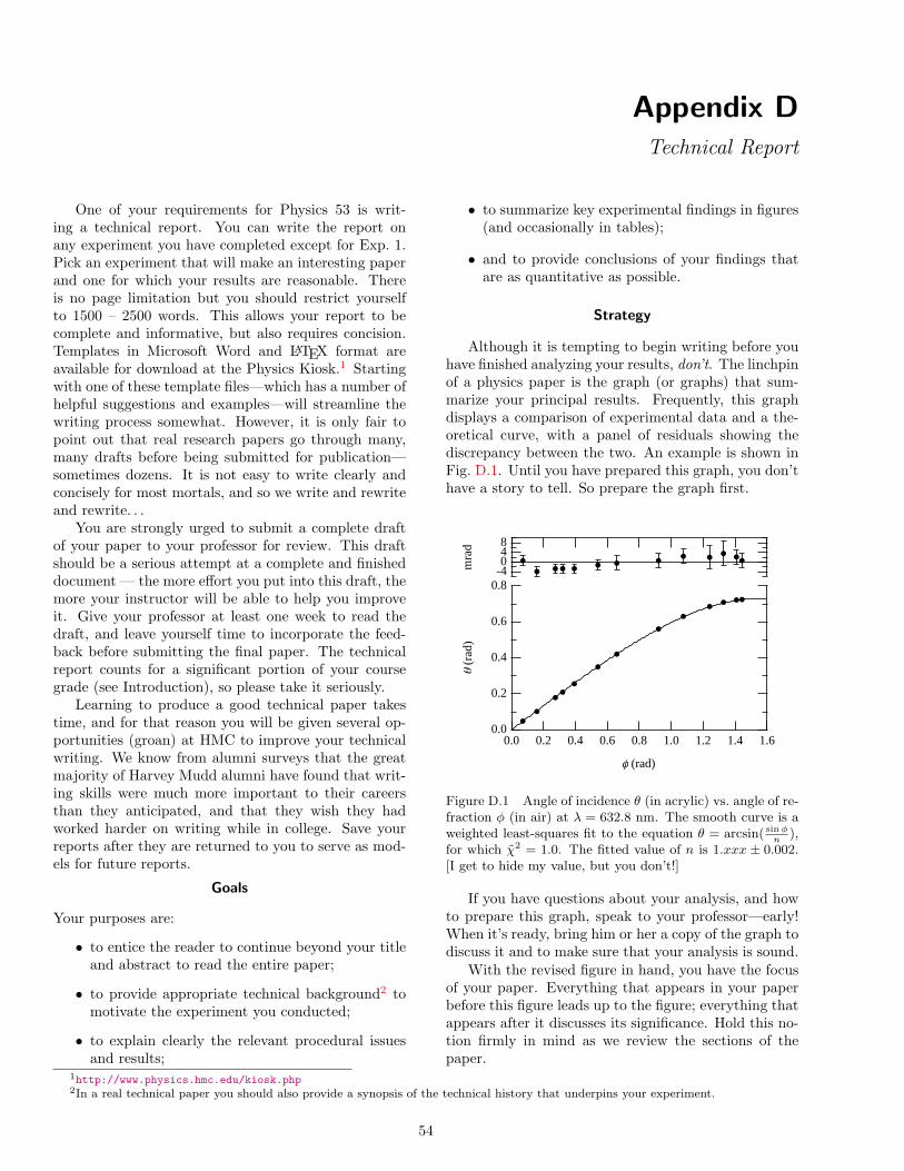
Appendix DTechnical Report

One of your requirements for Physics 53 is writ-ing a technical report. You can write the report onany experiment you have completed except for Exp. 1.Pick an experiment that will make an interesting paperand one for which your results are reasonable. Thereis no page limitation but you should restrict yourselfto 1500 – 2500 words. This allows your report to becomplete and informative, but also requires concision.Templates in Microsoft Word and LATEX format areavailable for download at the Physics Kiosk.1 Startingwith one of these template files—which has a number ofhelpful suggestions and examples—will streamline thewriting process somewhat. However, it is only fair topoint out that real research papers go through many,many drafts before being submitted for publication—sometimes dozens. It is not easy to write clearly andconcisely for most mortals, and so we write and rewriteand rewrite. . .

You are strongly urged to submit a complete draftof your paper to your professor for review. This draftshould be a serious attempt at a complete and finisheddocument — the more effort you put into this draft, themore your instructor will be able to help you improveit. Give your professor at least one week to read thedraft, and leave yourself time to incorporate the feed-back before submitting the final paper. The technicalreport counts for a significant portion of your coursegrade (see Introduction), so please take it seriously.

Learning to produce a good technical paper takestime, and for that reason you will be given several op-portunities (groan) at HMC to improve your technicalwriting. We know from alumni surveys that the greatmajority of Harvey Mudd alumni have found that writ-ing skills were much more important to their careersthan they anticipated, and that they wish they hadworked harder on writing while in college. Save yourreports after they are returned to you to serve as mod-els for future reports.

Goals

Your purposes are:

• to entice the reader to continue beyond your titleand abstract to read the entire paper;

• to provide appropriate technical background2 tomotivate the experiment you conducted;

• to explain clearly the relevant procedural issuesand results;

• to summarize key experimental findings in figures(and occasionally in tables);

• and to provide conclusions of your findings thatare as quantitative as possible.

Strategy

Although it is tempting to begin writing before youhave finished analyzing your results, don’t. The linchpinof a physics paper is the graph (or graphs) that sum-marize your principal results. Frequently, this graphdisplays a comparison of experimental data and a the-oretical curve, with a panel of residuals showing thediscrepancy between the two. An example is shown inFig. D.1. Until you have prepared this graph, you don’thave a story to tell. So prepare the graph first.

0.8

0.6

0.4

0.2

0.0

q (

rad)

1.61.41.21.00.80.60.40.20.0

f (rad)

840

-4mra

d

Figure D.1 Angle of incidence θ (in acrylic) vs. angle of re-fraction φ (in air) at λ = 632.8 nm. The smooth curve is aweighted least-squares fit to the equation θ = arcsin( sin φ

n),

for which χ2 = 1.0. The fitted value of n is 1.xxx ± 0.002.[I get to hide my value, but you don’t!]

If you have questions about your analysis, and howto prepare this graph, speak to your professor—early!When it’s ready, bring him or her a copy of the graph todiscuss it and to make sure that your analysis is sound.

With the revised figure in hand, you have the focusof your paper. Everything that appears in your paperbefore this figure leads up to the figure; everything thatappears after it discusses its significance. Hold this no-tion firmly in mind as we review the sections of thepaper.

1http://www.physics.hmc.edu/kiosk.php2In a real technical paper you should also provide a synopsis of the technical history that underpins your experiment.

54

APPENDIX D. TECHNICAL REPORT

Sections of a Technical Paper

The organization of a technical report follows a for-mulaic pattern, which is illustrated in Table D.1. Theelements of the paper are listed in the order in whichthey appear in the paper, not the order in which youshould write them! Although the abstract appears thirdon the list, you should probably leave it to the very last.Abstracts must be extremely concise and they can be achallenge to write. It is better to build momentum bywriting some of the easier sections first.

Theory

Assuming that you have completed the analysis ofyour data, and that you have prepared the figure(s) thatsummarize your results, I recommend beginning withthe theory section. For a Physics 53 technical report,this is apt to be a concise presentation of the theoryfrom the laboratory manual. Write for an educated per-son who understands mathematics and who has somescience background, but who has not conducted the ex-periment you did. The theory section should acquaintor remind your audience of the crucial theoretical back-ground to your experiment, without attempting to fillin all the steps. Make sure to define all symbols you em-ploy, and to explain the mathematics in plain English.Omit steps in a derivation that are merely algebraicmanipulations.

Number equations so that you can refer to them

later in the text. Remember that variables are set initalics (x), but functions and numbers are set in Roman(upright) font:

f(x) = sin(2x+ φ) (D.1)

If you are using Microsoft Word, be sure to use theEquation Editor to enter equations in proper format.You can find it at Insert | Object, and then selectingMicrosoft Equation 3.0 or something similar from thelist of objects. If you get tired of running this gauntlet,you can assign this task to a tool in the toolbar and/or akey combination using the Tools | Customize. . . com-mand.

Experiment

In writing this section you should have in mind areader who has your background in physics and is fa-miliar with typical laboratory apparatus, but has noknowledge of the specific experiment you are describingand probably has no intention of repeating it. There-fore, you should describe your experimental apparatusand the procedures you followed only insofar as it isnecessary for him or her to understand how you madeyour measurements. A careful drawing of the apparatusis often useful here.

In this regard it is important for you to understandthe distinction between a technical report and a labo-

Table D.1: Elements of a technical paper.Title

Author author’s nameauthor’s institution or companydate of submission

Abstract Summary of the principal facts and conclusions of the paper. Usually lessthan 100 words.

Introduction Concise discussion of the subject, scope, and purpose of the experiment.It should be accessible to the educated non-expert.

Theory Succinct development of the theory related to the experiment.

Experimentalmethods

Brief description of experimental apparatus and procedures.

Results Summary of important data and results, using figures (graphs) whereverpossible. Include error estimates for all relevant quantities. Note thatdata are typically presented graphically, not in tabular form, althoughthere are exceptions. If you feel a table is more appropriate, discuss thiswith your instructor.

Discussion orConclusions

Further analysis and discussion of results. Specific conclusions.Recommendations if needed. “Graceful termination.”

References The complete list of sources cited in the text.

August 1, 2005 55 Physics 53 Lab Manual

APPENDIX D. TECHNICAL REPORT

ratory manual. The latter is designed primarily to giveinstructions on how an experiment is to be carried out,while the former describes to the reader what the au-thor has done. Though it is sometimes necessary in atechnical report to describe the procedures that werefollowed in carrying out the experiment, such materialshould be kept to a minimum, and under no circum-stances should it instruct the reader as though he orshe were a student in a laboratory.

Data and Results

State first (or show first) your data before providingan interpretation. If you averaged 10 measurements ofthe pendulum period, simply state that the average of10 measurements was 1.87 s with a standard error of0.08 s.3

Usually, you will present your data in graphicalform, as in Fig. D.1. Occasionally, a table is more ap-propriate. However, do not display raw data in a table.

Figures and tables must be introduced and discussedin the text; they cannot be placed “inline” with thetext, and they certainly cannot be used to begin a sec-tion. Examples of the proper way to introduce figuresabound in this manual.

Some form of error analysis should be included withyour results, and the uncertainty of the final resultshould be stated clearly. The analysis of errors must bethorough and convincing. Your goal should be to per-suade a skeptical reader that your quantitative resultsare believable. This will often require a more thoroughanalysis of experimental errors than was done in yourlab notebook.

Discussion and Conclusions

This section will often contain further analysis anddiscussion of your results in order to support and clar-ify your conclusions. Your final conclusions shouldbe quantitative, precise, and specific, but they shouldnot be simply a summary of the experimental results.Rather, they should be convictions arrived at on thebasis of evidence previously presented and analyzed.

Until this section, the paper has grown progressivelynarrow, beginning with a broad introduction and taper-ing down to the nitty-gritty of your actual experiment.Once you have presented your most careful analysis, itis time to open up the discussion again, placing yourwork in a broader context. Make sure that you fulfillany promise you make to the reader in the Introductionas to what your paper would demonstrate or prove. Youmay want to include suggestions for further work.

Introduction

The Introduction needs to apprise the reader quicklyof the topic and scope of the paper, to engage the

reader, and to persuade her or him to continue read-ing. It may be the most challenging part of the paperto write. The first paragraph of the Introduction isparticularly critical, since it plays a major role in de-termining the reader’s attitude toward the paper as awhole. You will probably need to rewrite this sectionmore than other sections.

• Make the precise subject of the paper clear rel-atively early in the Introduction. You shouldassume your reader is someone with essentiallyyour background in physics but with no particu-lar knowledge of the experiment you performed.Thus you should include background materialonly to the extent necessary for the reader to un-derstand your statement of the subject of the pa-per and to appreciate the scientific reasons foryour doing the experiment to be described.

• State the purpose of the paper clearly. This state-ment should orient the reader with respect to thepoint of view and emphasis of the report and whathe should expect to learn from it. A well-doneIntroduction will also be of great help to you inproviding a focus for your writing and in drawingyour final conclusions (see below).

• Indicate the scope of the paper’s coverage of thesubject. State somewhere in the introductoryparagraphs the limits within which you treat thesubject. This definition of scope may include suchtopics as whether the work described was experi-mental or theoretical (In this particular case, thework is almost certainly experimental), the exactaspects of the general subject covered by the pa-per, the ranges of parameters explored, etc.

An example is given below in the section on passivevoice.

Abstract

The abstract should be a concise and specific sum-mary of the entire paper. It should be as quantitativeas possible and include important results and conclu-sions. Including all this in less than 100 words takescareful thought (and probably considerable rewriting).An example:

The speed at which light propagates through airat room temperature and atmospheric pressure wasstudied using a time-of-flight technique. A value of(2.995± 0.003)× 108 m/s was obtained, with the dom-inant error arising from the bandwidth of the oscillo-scope used to observe the light pulses. This value isconsistent with literature values for c and the refractiveindex of air.

3You may also report this result as (1.87± 0.08) s. Note that “standard error” and “standard deviation of the mean” are synonyms.

Physics 53 Lab Manual 56 August 1, 2005

APPENDIX D. TECHNICAL REPORT

References

Oy vey! Reference formatting is one of the dumb-est things in technical writing. Your paper should havereferences to published literature, where appropriate,but the format of those references as they appear instandard physics journals exhibits a remarkable (andpointless) variety. Every journal seems to have its ownpreferred way of doing things. Physical Review uses onestyle, except for Physical Review B, which uses a differ-ent one. Neither includes article titles, although IEEEstyle does. Physical Review used to put references atthe bottom of the page; now they appear as endnotesand all you see in the body of the text is a number inbrackets (or a superscripted number, in Phys. Rev. B).Neither approach is as civilized and useful as an (au-thor, date, page) in-text citation style, which is sadlyuncommon in physics publishing.4 Unless your profes-sor tells you otherwise, you may use either numbers or(author, date, page) citations in the text of your report.No matter what the format, though, the complete ref-erence must appear in the list of references at the end.If you use a numeric style, subsequent references to thesame source should use the same number, and the listof references should appear in the order of first cita-tion. For the (author, date, page) format, alphabetizethe references by author.

• No item should appear in the list of referenceswithout specific citation within the body of thetext.

• Cite published and commonly available sources(not the lab manual).

In the References section at the end of the paper,include the complete bibliographic information for eachof the cited works. Following is a list of references stylesthat roughly follow the American Institute of PhysicsStyle Manual. Note that the titles of majors works areitalicized, and volume numbers are set in boldface.

1. (journal article) Gale Young and R .E. Funderlic,J. Appl. Phys. 44 (1973) 5151.

2. (translated journal article) V. I. Kozub, Fiz. Tekh.Poluprovodn. 9 (1975) 2284 [Sov. Phys. Semi-cond. 9 (1976) 1479].

3. (book) L. S. Birks, Electron Probe Microanalysis,2nd ed. (Wiley, New York, 1971), p. 40.

4. (book section) D. K. Edwards, in Proceedings ofthe 1972 Heat Transfer and Fluid Mechanics In-stitute, Edited by Raymond B. Landis and Gary J.

Hordemann (Stanford University, Stanford, CA,1972), pp. 71-72.

5. R. C. Mikkelson (private communication).

6. James B. Danda, Ph.D. thesis, Harvard Univer-sity, 1965.

Passive Voice

In The Elements of Style, Strunk and White sug-gest using the active voice as much as possible. Thisis a worthy goal in scientific writing, but often the roleof the investigator is irrelevant to the topic at hand.Because the passive voice emphasizes the phenomenonnot the investigator, it is frequently more appropriate inscientific writing. Compare the following introductoryparagraphs, the first taken from a student’s technicalreport, and the second a rewritten version:

By running a current through a coil of wire, we canproduce a magnetic field which will deflect the needleof a compass. When we have done this, we can take abar magnet and position it such that the needle is nolonger deflected. Once this has been done, we need onlyto measure the distance from the needle’s center to themagnet. Using this and the properties we have alreadymeasured from the magnet and the coils, we can cal-culate the current through the loop. Because we onlytook measurements of mass, length, and time we havedetermined a value for current not based on any otherelectrical or magnetic quantities. [Emphasis added.]

Hans Christian Oersted discovered in 1820 that acurrent flowing in a wire generates a magnetic fieldproportional to the current.1 By comparing this fieldto that produced by a calibrated permanent magnet,and by using a geometry in which the constant of pro-portionality between field and current can be readilycalculated, it is possible to measure the current—anelectrical quantity—by measuring only the mechanicalquantities mass, length, and time. C. F. Gauss firstproposed a technique for making such an absolute de-termination of current in 1823.2 We report here a mod-ification of his technique which yields current measure-ments having an accuracy of 1%.

In my opinion, the use of the first person in the firstparagraph does not add useful information; rather, itdetracts from the message that these phenomena ex-ist independent of the observer. The second paragraphuses some active voice and some passive voice, throwsin some historical information, and keeps the discussionconceptual, as befits an introduction.

4Bibliographic database software, such as Endnote or ProCite, can simplify the task of reference formatting, but is apt to be overkillfor the technical report. These programs understand the styles of a vast number of publications, and can format the bibliographic infor-mation in their databases to match the requirements of whichever publication you target. You can also store notes and other informationassociated with references in your bibliography, and reuse this information in multiple publications. For extended research projects, suchsoftware can be extremely convenient.

August 1, 2005 57 Physics 53 Lab Manual

APPENDIX D. TECHNICAL REPORT

Make no mistake: good writing of any kind, whethertechnical or not, requires practice and a willingness torewrite. Simply put, it’s hard!

Do’s and Don’t’s

Do’s

1. Double space the report, except for the abstract.

2. Divide the report into clearly labeled sections(Abstract, Introduction, Theory, . . . ).

3. Number all pages.

4. Place tables and figures as soon as possible afterthey are referred to in the text.

5. Give each table and figure a complete title and/orself-descriptive caption.

6. Give each table and figure a complete title and/orself-descriptive caption.

7. Define all symbols used.

8. Number all equations. (Place numbers near right-hand margin.) Each equation should be on a sepa-

rate line. Use complete sentences and fit all equa-tions into the sentences that introduce them.

9. Avoid imprecise, vague, or unclear language.Carefully define your terms and use them consis-tently. Avoid jargon and excessive abbreviations.

10. Tell a story. Organize your information so thatthe narrative proceeds smoothly and logically.

11. Use SI units unless there is a compelling reasonnot to. That is, use µm or nm, but not A.

Don’t’s

1. Do not repeat every sordid detail from a lab diary;report the logically crucial ones.

2. Do not distort unpleasant realities; call it like itis. Don’t attempt to cover up flaws in your data;do explain departures from theory when you can.

3. Do not scan someone else’s figure.

Technical Typography

1. Algebraic symbols (variables and constants)should be italicized. E = mc2, not E = mc2.In Microsoft Word, modify the fonts yourself oruse the Equation Editor. In LATEX type inlineequations inside dollar signs: $E = mc^2$.

2. Subscripts are italicized when they refer to sym-bols, but Roman when they are words

Bbar = Bx tanφ (D.2)

LATEX: B_\rm bar = B_x \tan\phi

3. Vectors are written in boldface (usually not itali-cized), but their magnitude is set in italics. Func-tions such as sine are not italicized.

τ = M×B or ~τ = ~M× ~B

τ = MB sin θ

LATEX: \boldsymbol\tau =\mathbfM \times \mathbfB

4. Refer to the second figure as “Fig. 2”. Write out“Figure 2” if this starts the sentence.

5. Figures should have informative captions. Mostpeople “read” a paper by looking at the title, ab-stract, and figures. By making the figures clearand the captions informative, you increase yourchances of getting the reader to read the text.

6. Number pages.

7. Do not underline. Book titles should be italicized.Volume numbers should appear in bold. Exam-ple: D. Quayle, J. Irrepro. Res. 21 (1996) 1234.[Note that “1234” is the page number of the arti-cle.]

8. Get your symbols for units right: “Hz” not “hz”,“Ω” not “Ohm”, “30” not “30 degrees”. Note:units are not pluralized: don’t use “secs”, “hrs”,etc. Never ever screw up the capitalization of SIprefixes: there’s a crucial difference between MHzand mHz.

9. Abbreviations (e.g., RLC, rms, etc.) must be de-fined when first used (except in a title, where theyshould usually be avoided).

10. A number and the unit that modifies it should beseparated by a (nonbreaking) space (e.g., 50.1 Hz,not 50.1Hz). The space should be a hyphen whenthe number-unit phrase functions as an adjectivebefore the verb (e.g., A 50-Hz signal was appliedacross points A and B). In Microsoft Word, headto the Insert | Symbol command and select theSpecial Characters tab to find how to insert anonbreaking space. In LATEX it is typed with atilde (~).

Physics 53 Lab Manual 58 August 1, 2005

APPENDIX D. TECHNICAL REPORT

11. To type a multiplication symbol in MicrosoftWord, use the Insert | Symbol and select Symbolfont to get the palette of mathematical symbols.Then select the multiplication sign and click In-sert. In LATEX use the \times command in mathmode.

12. If you use superscripts as endnote markers, theyshould appear after the punctuation mark (e.g.,“. . . is given by the Biot-Savart law.1”) If you usenumbers in brackets, they go before (“. . . is givenby the Biot-Savart Law [1].”).

13. Do not start a sentence with a symbol.

14. Doan furget two speel cheque. An prufreed.Swapping papers with a friend for proofreadingis often very helpful.

Proofing marks

stet. Latin for “let it stand.” Leave as it was (Iscrewed up and marked something and thendecided to “unmark” it).

awk. awkward—rewrite the sentence or paragraphit. italics

August 1, 2005 59 Physics 53 Lab Manual