PHYS 642

Radiative Processes in Astrophysics

Winter term 2009

– 2 –

1. Radiative Transfer

These are notes for the first part of PHYS 642 Radiative Processes in Astrophysics. The

idea is to get as far as we can without worrying about the microphysics by which radiation is

emitted, absorbed, or scattered. We will develop a formalism to follow the radiation from its

source to the observer through intervening material, taking into account absorption, emis-

sion, and scattering, and discuss the properties of thermal radiation. Examples covered are

radiative di↵usion in stellar interiors and the Rosseland mean opacity, the grey atmosphere

as the simplest example of a stellar atmosphere, the spectrum of an atmosphere and limb

darkening, and the origin of emission and absorption lines.

1.1. The specific intensity and its moments

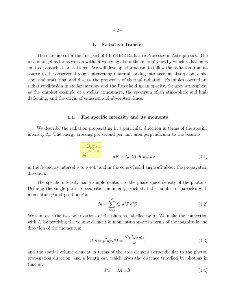
We describe the radiation propagating in a particular direction in terms of the specific

intensity I⌫ . The energy crossing per second per unit area perpendicular to the beam is

dE = I⌫ dA dt d⌦ d⌫ (1.1)

in the frequency interval ⌫ to ⌫+d⌫ and in the cone of solid angle d⌦ about the propagation

direction.

The specific intensity has a simple relation to the phase space density of the photons.

Defining the single particle occupation number f↵ such that the number of particles with

momentum ~p and position ~x is

dn =2X

↵=1

f↵ d3~x d3~p. (1.2)

We sum over the two polarizations of the photons, labelled by ↵. We make the connection

with I⌫ by rewriting the volume element in momentum space in terms of the magnitude and

direction of the momentum,

d3~p = p2dp d⌦ =h3⌫2d⌫ d⌦

c3

(1.3)

and the spatial volume element in terms of the area element perpendicular to the photon

propagation direction, and a length cdt, which gives the distance travelled by photons in

time dt,

d3~x = dA c dt. (1.4)

– 3 –

This gives

dn =X

↵

f↵h3

h⌫3

c2

dA dt d⌦ d⌫ (1.5)

and therefore

I⌫ ⌘

X

↵

f↵h3

h⌫3

c2

. (1.6)

The energy density of the radiation is

U =

Zd3~p

X

↵

f↵h⌫ =1

c

ZIv d⌫ d⌦ (1.7)

from which we see that

U⌫ =1

c

ZI⌫ d⌦. (1.8)

We can also write an expression for the energy flux ~F . In the x-direction, for example,

Fx =

Zd3~pX

↵

f↵ vx h⌫ (1.9)

where we construct the flux by multiplying the number density of particles by the velocity

in the x-direction and the quantity being carried, here energy. If ✓ is the angle with respect

to the photon propagation direction, then

Fx =

Zd3~pX

↵

f↵ h⌫c cos ✓ =

ZI⌫ d⌫ d⌦ cos ✓ (1.10)

Similarly, we can derive the pressure of the radiation by calculating the momentum flux

across a unit area. The flux of x-momentum in the x-direction is

Pxx =

Zd3~pX

↵

f↵ vx px =

Zd3~pX

↵

f↵ h⌫ cos2 ✓ =1

c

ZI⌫ d⌫ d⌦ cos2 ✓ (1.11)

We see that the energy density, pressure, and flux can be expressed in terms of the

zeroth, first, and second moments of the radiation field,

cU⌫

4⇡= J⌫ =

1

4⇡

ZI⌫d⌦ =

1

2

Z1

�1

dµ I⌫(µ) (1.12)

F⌫

4⇡= H⌫ =

1

4⇡

ZI⌫ cos ✓ d⌦ =

1

2

Z1

�1

dµ µI⌫(µ) (1.13)

cP⌫

4⇡= K⌫ =

1

4⇡

ZI⌫ cos2 ✓ d⌦ =

1

2

Z1

�1

dµ µ2I⌫(µ) (1.14)

– 4 –

where the integrals over µ are for an axially symmetric radiation field, where d⌦ = 2⇡ dµ

with µ = cos ✓. The quantity J⌫ is known as the mean intensity.

Let’s do some simple examples. An isotropic radiation field has I⌫ constant for photons

propagating in all directions. Then

cU⌫

4⇡= J⌫ = I⌫ =

3cP⌫

4⇡(1.15)

or

P⌫ =1

3U⌫ . (1.16)

The flux vanishes for integration over all solid angles. The flux from a surface is given by

integrating over a hemisphere in solid angle,

F⌫ = ⇡I⌫ . (1.17)

Another example is a unidirectional radiation field, e.g. I⌫ = I0

�(µ). This gives P⌫ = U⌫ in

contrast to the result for an isotropic radiation field. In an atmosphere as we move towards

the surface, the radiation field becomes more and more outwards directed, and P⌫/U⌫ goes

from 1/3! 1. Keeping track of this variation is important in modeling stellar atmospheres.

1.2. Thermal radiation

An important case is when the radiation is in thermal equilibrium at temperature T .

Then the photon distribution function is given by the Bose-Einstein distribution with zero

chemical potential (µ = 0)

h3f↵ =1

eh⌫/kBT� 1

(1.18)

the same for both spin states ↵, giving

Iv ⌘ B⌫(T ) =2h⌫3

c2

1

eh⌫/kBT� 1

(1.19)

which defines the Planck distribution B⌫(T ) or blackbody spectrum. The two limits h⌫ �

kBT and h⌫ ⌧ kBT both have names. The Rayleigh-Jeans part of the spectrum at low

frequency is given by

B⌫ =2⌫2

c2

kBT / ⌫2. (1.20)

This formula can be obtained by counting the photon modes and assuming each has kBT of

energy in thermal equilibrium. Taken to large frequency, this predicts infinite energy in the

photon field, the so-called ultraviolet catastrophe. The resolution is in the quantization of

– 5 –

the photon energy spectrum. At high frequencies, the photon energy becomes much greater

than the thermal energy h⌫/kBT , and the occupation number is exponentially suppressed,

giving the Wien tail

B⌫ =2h⌫3

c2

exp

✓�h⌫

kBT

◆. (1.21)

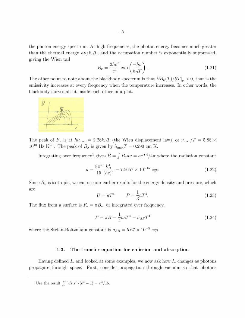
The other point to note about the blackbody spectrum is that @B⌫(T )/@T |⌫ > 0, that is the

emissivity increases at every frequency when the temperature increases. In other words, the

blackbody curves all fit inside each other in a plot.

The peak of B⌫ is at h⌫max

= 2.28kBT (the Wien displacement law), or ⌫max

/T = 5.88 ⇥

1010 Hz K�1. The peak of B� is given by �max

T = 0.290 cm K.

Integrating over frequency1 gives B =R

B⌫d⌫ = acT 4/4⇡ where the radiation constant

a =8⇡5

15

k4

B

(hc)3

= 7.5657⇥ 10�15 cgs. (1.22)

Since B⌫ is isotropic, we can use our earlier results for the energy density and pressure, which

are

U = aT 4 P =1

3aT 4. (1.23)

The flux from a surface is F⌫ = ⇡B⌫ , or integrated over frequency,

F = ⇡B =1

4acT 4 = �SBT 4 (1.24)

where the Stefan-Boltzmann constant is �SB = 5.67⇥ 10�5 cgs.

1.3. The transfer equation for emission and absorption

Having defined I⌫ and looked at some examples, we now ask how I⌫ changes as photons

propagate through space. First, consider propagation through vacuum so that photons

1Use the resultR10 dxx3/(ex

� 1) = ⇡4/15.

– 6 –

are neither created or destroyed. The single particle distribution function f↵ satisfies the

collisionless Boltzmann equation

1

c

@f

@t+ ~

k ·

~rf↵ = 0 (1.25)

where ~k is a unit vector giving the photon propagation direction. This is straightforward

to derive. The idea is that photons initially at position (~x, ~p) in phase space will be at

position (~x + ~kcdt, ~p) a time dt later. The photons conserve phase space volume as they

propagate. Setting the number of photons in a phase space volume d3~xd3~p constant implies

that f↵(~x, ~p, t) = f↵(~x + ~kcdt, ~p, t + dt). Equation (1.25) follows by a Taylor expansion.

Since I⌫ and f↵ are related by a constant factor, then

1

c

@I⌫

@t+ ~k ·

~rI⌫ = 0. (1.26)

There are two points to make about this equation. First, the first term is often much smaller

than the second term if the timescale for evolution of the system we’re interested in is

much longer than the light crossing time for that system. Second, in general photons are

not conserved but scattered, absorbed, and emitted and we account for these processes by

adding source and sink terms to the RHS. Define coordinate s along the photon path, we

then havedI⌫

ds= (sources)� (sinks). (1.27)

In general, we must solve a number of equations for I⌫ at di↵erent photon frequencies and

propagation directions. Emission and absorption of photons by matter are obvious sources

and sinks that we must include. Also, scattering moves photons from one direction to another

and perhaps from one frequency to another if it is inelastic.

The spontaneous emission coe�cient j⌫ is defined as the energy emitted per unit time,

volume, in a given direction and frequency, so that

dI⌫

ds= j⌫ (1.28)

with units erg cm�3 s�1 Hz�1 sterad�1. Often the emission process is isotropic, and it’s

useful to define an emissivity ✏⌫ , where

j⌫ =⇢✏⌫4⇡

(1.29)

(units of ✏⌫ are erg g�1 s�1 Hz�1). We’ll calculate j⌫ due to various physical processes later

in the course. Notice that locally where we can treat j⌫ as constant, the specific intensity

increases linearly due to emission.

– 7 –

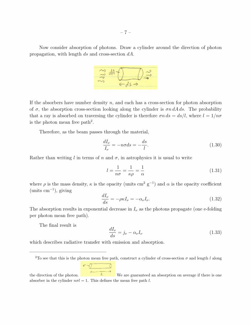
Now consider absorption of photons. Draw a cylinder around the direction of photon

propagation, with length ds and cross-section dA.

If the absorbers have number density n, and each has a cross-section for photon absorption

of �, the absorption cross-section looking along the cylinder is �n dAds. The probability

that a ray is absorbed on traversing the cylinder is therefore �n ds = ds/l, where l = 1/n�

is the photon mean free path2.

Therefore, as the beam passes through the material,

dI⌫

I⌫

= �n�ds = �ds

l. (1.30)

Rather than writing l in terms of n and �, in astrophysics it is usual to write

l =1

n�=

1

⇢=

1

↵(1.31)

where ⇢ is the mass density, is the opacity (units cm2 g�1) and ↵ is the opacity coe�cient

(units cm�1), givingdI⌫

ds= �⇢I⌫ = �↵⌫I⌫ . (1.32)

The absorption results in exponential decrease in I⌫ as the photons propagate (one e-folding

per photon mean free path).

The final result isdI⌫

ds= j⌫ � ↵⌫I⌫ (1.33)

which describes radiative transfer with emission and absorption.

2To see that this is the photon mean free path, construct a cylinder of cross-section � and length l along

the direction of the photon. We are guaranteed an absorption on average if there is oneabsorber in the cylinder n�l = 1. This defines the mean free path l.

– 8 –

1.4. Optical depth, source function, and Kircho↵ ’s theorem

We define the optical depth ⌧ by d⌧ = ↵ds = ⇢ds = ds/l, or

⌧(s)� ⌧(s0

) =

Z s

s0

↵(s)ds (1.34)

If ⌧ � 1 when integrated along a typical path in a medium, the medium is said to be optically

thick (most photons absorbed), whereas if ⌧ ⌧ 1 along a typical path, the medium is said

to be optically thin (most photons escape).

To get a sense of the size of the mfp as a function of density, we can estimate � ⇡ �T

where �T = 8⇡r2

0

/3 = 6.63 ⇥ 10�25 cm2 is the Thomson cross-section and r0

= e2/mec2

is the classical electron radius3. This cross-section is for Thomson scattering rather than

absorption, but gives a starting point for an estimate of an interaction cross-section. For a

gas of protons, the cross-section per gram is then

=�T

mp

= 0.40 cm2 g�1. (1.35)

The photon mfp is

l =1

n�=

0.5 Mpc

(n/cm�3)(1.36)

or

l =1

⇢=

2.5 cm

(⇢/g cm�2). (1.37)

The first case is a typical interstellar medium (ISM) density, the second case is for the mean

density of the Sun. For the Sun, the mean free path is a factor ⇠ 1011 smaller than the

radius of the star, so that the solar interior is extremely optically thick. For the ISM, the

mean free path we estimate is larger than the size of the Galaxy. Of course, we haven’t

included the correct opacity sources for optical photons travelling through the ISM, but still

this estimate makes the point that at ISM densities the mfp can be large.

In terms of optical depth, the transfer equation is

dI⌫

d⌧⌫=

j⌫

↵⌫

� I⌫ = S⌫ � I⌫ (1.38)

where we define the source function S⌫ ⌘ j⌫/↵⌫ .

3Note that in cgs, the electron charge is e = 4.8032⇥ 10�10 cgs.

– 9 –

The general solution of the transfer equation is4

I⌫(⌧⌫) = I⌫(0)e�⌧⌫ +

Z ⌧⌫

0

e�(⌧⌫�⌧ 0⌫)S⌫ (⌧ 0⌫) d⌧ 0⌫ . (1.39)

Each term has a simple physical interpretation. The first term describes absorption of the

incident radiation I⌫(0). The second term is an integral over the emitted photons given by

the source function, and a factor to include absorption of those emitted photons as they

propagate to optical depth ⌧⌫ .

As a simplified case, consider S =constant. Then the solution is

I⌫(⌧⌫) = I⌫(0)e�⌧⌫ + S⌫

�1� e�⌧⌫

�= S⌫ + e�⌧⌫ (I⌫(0)� S⌫) (1.40)

which shows that for large optical depths, I⌫ ! S⌫ . If initially I⌫ > S⌫ , then photons are

absorbed from the beam until I⌫ = S⌫ . Similarly, if I⌫ < S⌫ initially, then photons are added

to the beam until I⌫ = S⌫ . For small optical depth, I⌫(⌧⌫) ⇡ I⌫(0)(1� ⌧⌫) + ⌧⌫S⌫ .

An extremely important result is Kircho↵ ’s law, which states that a material in ther-

modynamic equilibrium at temperature T has

j⌫ = ↵⌫B⌫(T ) (1.41)

or

S⌫ = B⌫(T ). (1.42)

One way to see that this must be the case is to consider an object placed inside a thermal

cavity and allowed to come into equilibrium with it. It must replace any radiation it absorbs,

frequency by frequency.

A true blackbody has ↵⌫ constant, independent of frequency (a “perfect absorber”

absorbs all frequencies equally), and so has j⌫ / B⌫ . But this is not true for real materials,

which have an emissivity weighted by a non-constant absorption coe�cient. At frequencies

which are readily absorbed, the emissivity is high, and vice versa. An example of this is

emission lines from thermal optically thin gas (e.g. in the chromosphere of the Sun). The

absorption coe�cient ⌫ is larger at the frequencies of line transitions, and therefore so is

the emissivity.

4To see this, first take out the expected e�⌧ behavior by defining f = I⌫

e⌧ , and g = Se⌧ . Then df/d⌧ = g

can be integrated to give eq. [1.39].

– 10 –

1.5. Examples

1.5.1. Stellar interiors

Let’s consider optically thick regions such as stellar interiors. A good assumption is often

local thermodynamic equilibrium (LTE), in which the degrees of freedom associated with the

particles (e.g. atomic energy levels) are characterized by their values in thermodynamic

equilibrium (TE) at temperature T . In this case, S⌫ = B⌫(T ). The di↵erence from full TE is

that the radiation field in general does not have a Planck distribution, I⌫ = B⌫(T ). However,

our solution for the radiative transfer equation tells us that I⌫ ! B⌫ for optically thick LTE

material.

We first write ds in terms of the radial coordinate r, as ds = dr cos ✓ = µdr for a photon

propagating at angle ✓ to the radial direction. Then

µdI⌫

dr= j⌫ � ↵⌫I⌫ . (1.43)

Since the optical depth increases inwards, it makes sense to define the radial optical depth

as d⌧⌫ = �↵⌫dr, and so

µdI⌫

d⌧⌫= �S⌫ + I⌫ (1.44)

where the factor of µ on the LHS accounts for the fact that ⌧⌫ is the radial optical depth.

Next, we take the moments of equation (1.44). Integrating over solid angle gives

1

4⇡

dF⌫

d⌧⌫= �S⌫ + J⌫ (1.45)

and multiplying by µ and integrating gives

cdP⌫

d⌧⌫= F⌫ . (1.46)

We have assumed S⌫ is isotropic so thatR

d⌦µS⌫ = 0.

In a stellar interior, we already mentioned the fact that ⌧ � 1, and therefore we expect

I⌫ ⇡ B⌫ . However, there must be some anisotropy in the radiation field since the photons

transport heat outwards. Therefore

I⌫ = B⌫(T ) + (small anisotropic part) (1.47)

Now look at equation (1.46). The flux F⌫ must come from the anisotropic part of I⌫ , but

the pressure is mostly set by the isotropic part, P⌫ ⇡ 4⇡B⌫/3c. Therefore

F⌫ = �4⇡

3⇢⌫

dB⌫

dT

dT

dr. (1.48)

– 11 –

Integrating over frequency gives the total flux

F = �4⇡

3⇢

dT

dr

Zd⌫

1

⌫

dB⌫

dT. (1.49)

Next, we define the Rosseland mean opacityZ

d⌫dB⌫

dT

�1

R

=

Zd⌫

1

⌫

dB⌫

dT

�. (1.50)

The factor on the LHS isZ

d⌫dB⌫

dT=

d

dT

Zd⌫B⌫ =

d

dT

✓acT 4

4⇡

◆(1.51)

and therefore we arrive at

F = �4acT 3

3R⇢

dT

dr(1.52)

the radiative di↵usion equation.

We see that radiation di↵uses down the temperature gradient, as would be expected.

We can rewrite equation (1.52) as

F = �1

3c l

d

dr

�aT 4

�(1.53)

exactly what we would have guessed from a kinetic theory approach. The 1/3 factor is the

usual factor from integration over angles, and the transported quantity is the photon energy

density aT 4. At a given location, the photons coming from deeper in the star are hotter (by

an amount ⇡ ldT/dr) than those coming from cooler regions above.

We can use equation (1.52) to understand the solar luminosity. We expect

L� ⇡ 4⇡R2F

⇡ 4⇡R2

1

3cl

aT 4

c

R

⇡

✓4⇡R3

3aT 4

c

◆✓cl

R2

◆. (1.54)

In the second line, we approximate d(aT 4)/dr ⇡ aT 4

c /R, where Tc is the central temperature.

In the last line, the first term is the total energy content in radiation in the solar interior.

In the second term, we are dividing by the time for a photon to random walk out of the

Sun. Recall that for a random walk, the total distance travelled is R =p

Nl where N is the

number of steps. Therefore the time to escape is Nl/c = R2/lc = tesc

, and

L� ⇡E�

tesc

. (1.55)

– 12 –

Let’s plug in some numbers: the central density of the Sun is ⇢ ⇡ 150 g cm�3 which gives

l/R ⇡ 10�13 (see eq. [1.37]). The light travel time is R/c ⇡ 2 s, and therefore tesc

⇡ 106 years.

The luminosity of the Sun L� = 4⇥1033 erg s�1. Putting this together gives Tc ⇡ 9⇥106 K.

Not bad, the actual value is 1.5⇥ 107 K.

1.5.2. Grey atmosphere: temperature profile, limb darkening

Next, we consider the solution of the radiative transfer equation in the stellar atmo-

sphere, in which the optical depth drops from ⌧ � 1 to ⌧ ⌧ 1. The simplest case is a grey

atmosphere, in which “grey” refers to a frequency-independent opacity ⌫ = . Equation

(1.45) integrated over frequency is

1

4⇡

dF

d⌧= �S + J (1.56)

which for a constant flux F implies that we must have S = J . Similarly, the frequency-

integrated equation (1.46),

cdP

d⌧= F (1.57)

gives the simple result P = (F/c)(⌧ + ⌧0

). To close these equations, we make the Eddington

approximation that U = 3P or 3P = 4⇡J/c. Then,

S = J =3cP

4⇡=

3F

4⇡(⌧ + ⌧

0

). (1.58)

To find the constant ⌧0

, we solve the radiative transfer equation for I(⌧) and then use it

to find the flux F at the surface. Only for the correct choice of ⌧0

is the solution self-consistent

in this way. The specific intensity is

I(⌧, µ) =

Z 1

⌧

e�(⌧�⌧ 0)/µS (⌧ 0)d⌧ 0

µ. (1.59)

Substituting our expression for S gives I(0) = (3F/4⇡)(⌧0

+ µ) for µ > 0 and I(0) = 0 for

µ < 0. The flux at the surface can be found fromZ

1

0

2⇡µ dµ I(0), (1.60)

which is equal to F only if ⌧0

= 2/3.

If we assume LTE, then S = B, and therefore

B = S =3F

4⇡

✓⌧ +

2

3

◆(1.61)

– 13 –

but F = �T 4

e↵

and B = �T 4/⇡, giving

T 4 =3

4T 4

e↵

✓⌧ +

2

3

◆, (1.62)

the temperature profile of the grey atmosphere in the Eddington approximation. Note that

T = Te↵

at ⌧ = 2/3. This optical depth is often taken as the photosphere.

The specific intensity for arbitrary depth is (for outgoing rays, µ > 0)

I(µ, ⌧) =3F

4⇡

✓µ +

2

3+ ⌧

◆= B +

3Fµ

4⇡. (1.63)

This shows that at large optical depth, the anisotropic part of the specific intensity is ⇡ 1/⌧

of the isotropic part.

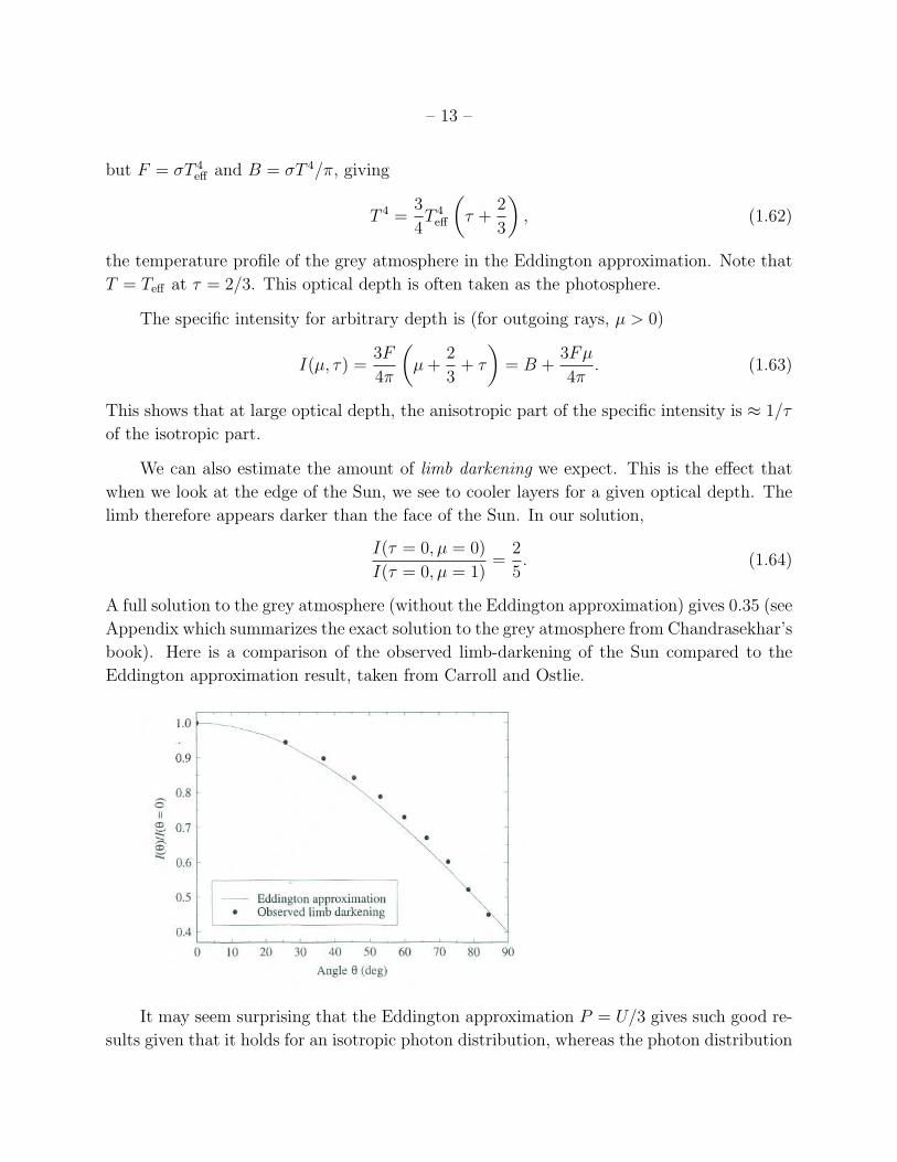
We can also estimate the amount of limb darkening we expect. This is the e↵ect that

when we look at the edge of the Sun, we see to cooler layers for a given optical depth. The

limb therefore appears darker than the face of the Sun. In our solution,

I(⌧ = 0, µ = 0)

I(⌧ = 0, µ = 1)=

2

5. (1.64)

A full solution to the grey atmosphere (without the Eddington approximation) gives 0.35 (see

Appendix which summarizes the exact solution to the grey atmosphere from Chandrasekhar’s

book). Here is a comparison of the observed limb-darkening of the Sun compared to the

Eddington approximation result, taken from Carroll and Ostlie.

It may seem surprising that the Eddington approximation P = U/3 gives such good re-

sults given that it holds for an isotropic photon distribution, whereas the photon distribution

– 14 –

is anisotropic in the stellar atmosphere. In fact, the Eddington approximation holds for more

general angular distributions of the photons. For example, if the photons are isotropic in

the outgoing and ingoing hemispheres, but with di↵erent intensities, the Eddington approx-

imation holds. Similarly, the Eddington approximation holds for the anisotropic intensity

I = a + bµ (or with additional terms as long as only odd powers of µ are included).

1.5.3. Spectrum of a grey atmosphere

Having calculated the temperature profile of the grey atmosphere, we can now go back

and calculate its spectrum if we assume LTE so that the source function is B⌫(T ) at each

depth. Then the outgoing specific intensity at the surface is

I⌫(0, µ) =

Z 1

0

e�⌧/µB⌫ (T (⌧))d⌧

µ(1.65)

where we can take T (⌧) as previously calculated using the Eddington approximation. The

emergent flux is

F⌫(0) =

Z1

0

dµ 2⇡µ I⌫(0, µ) (1.66)

=

Z1

0

dµ 2⇡µ

Z 1

0

e�⌧/µB⌫(T )d⌧

µ(1.67)

= 2⇡

Z 1

0

d⌧B⌫(T )

Z1

0

dµ e�⌧/µ (1.68)

= 2⇡

Z 1

0

d⌧B⌫(T )

Z 1

1

dx

x2

e�⌧x (1.69)

= 2⇡

Z 1

0

d⌧B⌫(T )E2

(⌧) (1.70)

where we have made the substitution x = 1/µ, and E2

(⌧) is an exponential integral5.

5Defined as En

(⌧) =R11 x�ne�⌧x dx. These functions occur often in analytic solutions to the radiative

transfer problem. Some properties (which are straightforward to prove) are: En

(x) ! e�x/x for x ! 1,E1(x) ! ln(1/x) as x ! 0, E

n

(x) ! 1/(n � 1) as x ! 0 (n > 1), (n � 1)En

(x) = e�x

� xEn�1(x),

dEn

/dx = �En�1(x), and

R10 dxE

n

(x) = 1/n. This last result can be used to show that eq. [1.70] gives thecorrect result for an isothermal atmosphere, F

⌫

= ⇡B⌫

(T ).

– 15 –

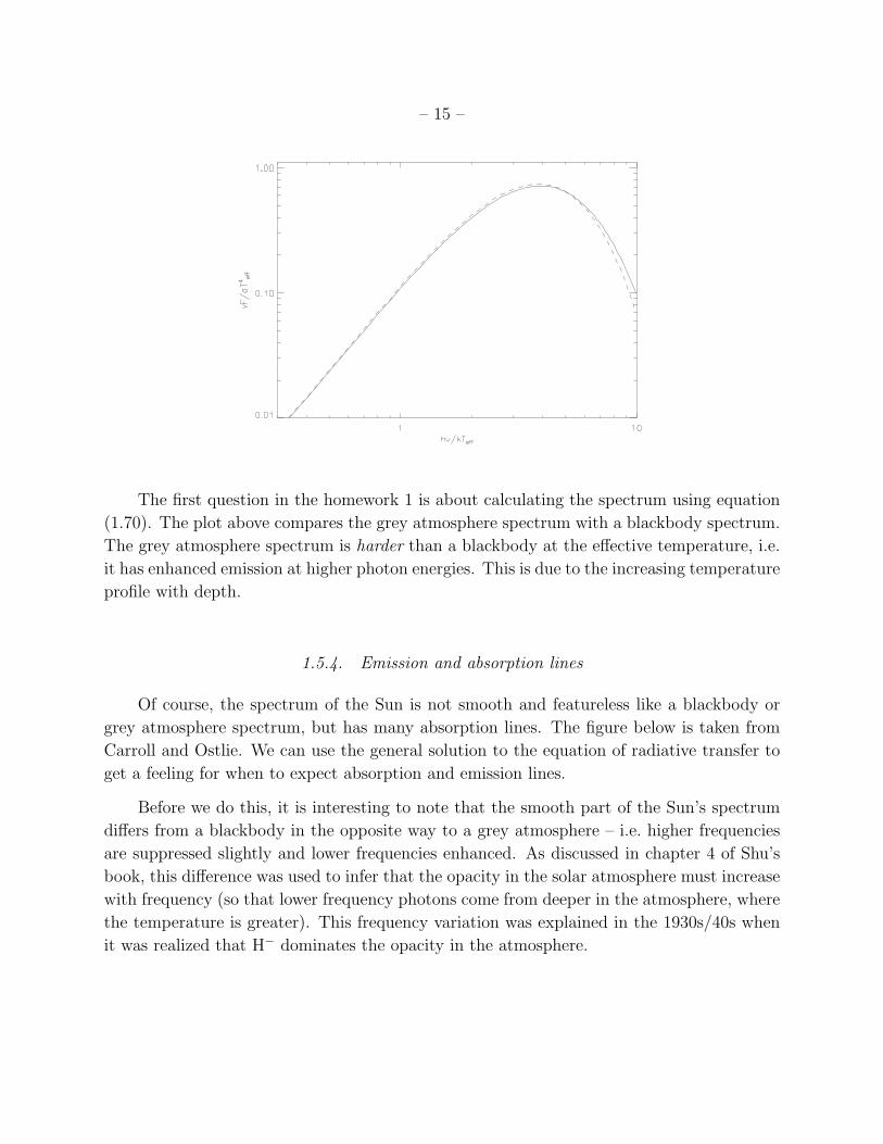
The first question in the homework 1 is about calculating the spectrum using equation

(1.70). The plot above compares the grey atmosphere spectrum with a blackbody spectrum.

The grey atmosphere spectrum is harder than a blackbody at the e↵ective temperature, i.e.

it has enhanced emission at higher photon energies. This is due to the increasing temperature

profile with depth.

1.5.4. Emission and absorption lines

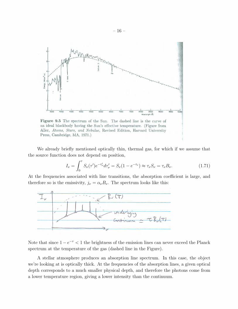
Of course, the spectrum of the Sun is not smooth and featureless like a blackbody or

grey atmosphere spectrum, but has many absorption lines. The figure below is taken from

Carroll and Ostlie. We can use the general solution to the equation of radiative transfer to

get a feeling for when to expect absorption and emission lines.

Before we do this, it is interesting to note that the smooth part of the Sun’s spectrum

di↵ers from a blackbody in the opposite way to a grey atmosphere – i.e. higher frequencies

are suppressed slightly and lower frequencies enhanced. As discussed in chapter 4 of Shu’s

book, this di↵erence was used to infer that the opacity in the solar atmosphere must increase

with frequency (so that lower frequency photons come from deeper in the atmosphere, where

the temperature is greater). This frequency variation was explained in the 1930s/40s when

it was realized that H� dominates the opacity in the atmosphere.

– 16 –

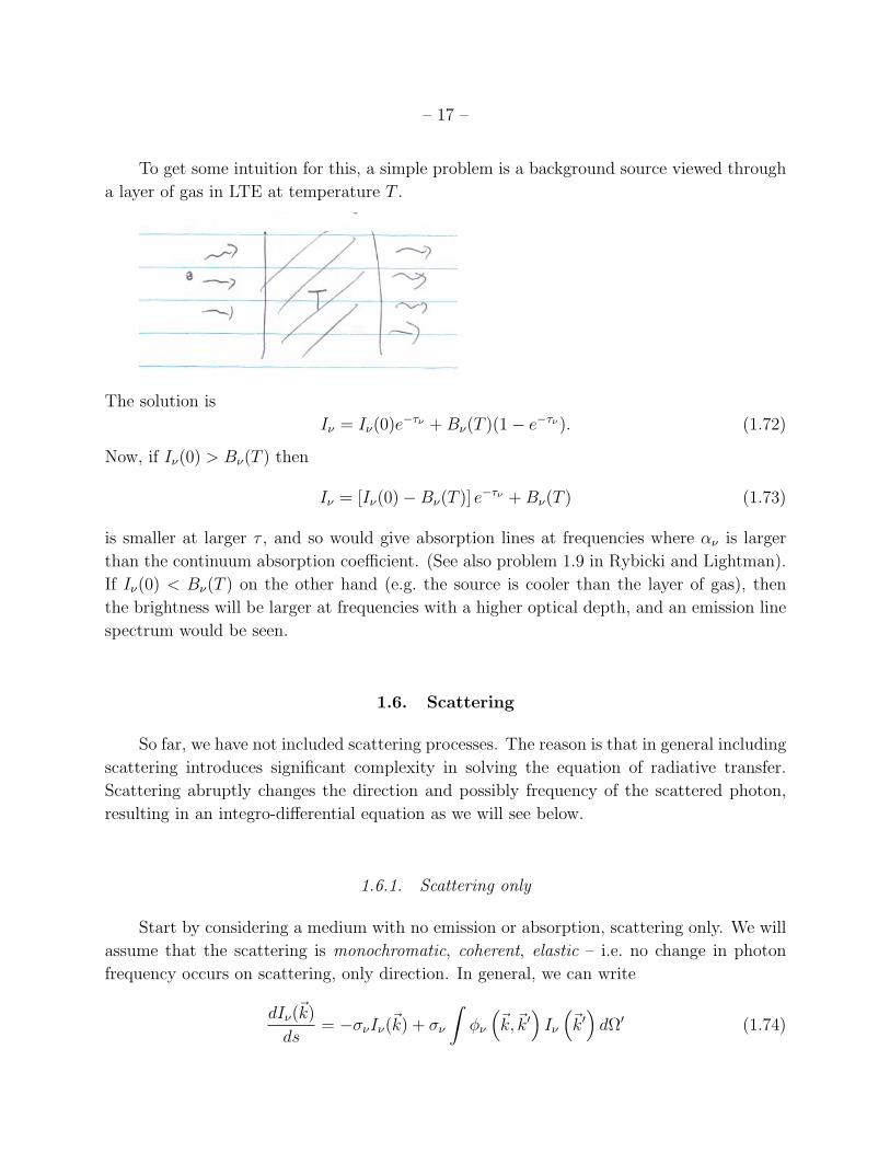
We already briefly mentioned optically thin, thermal gas, for which if we assume that

the source function does not depend on position,

I⌫ =

Z ⌧

0

S⌫(⌧0)e�⌧ 0⌫d⌧ 0⌫ = S⌫(1� e�⌧⌫ ) ⇡ ⌧⌫S⌫ = ⌧⌫B⌫ . (1.71)

At the frequencies associated with line transitions, the absorption coe�cient is large, and

therefore so is the emissivity, j⌫ = ↵⌫B⌫ . The spectrum looks like this:

Note that since 1� e�⌧ < 1 the brightness of the emission lines can never exceed the Planck

spectrum at the temperature of the gas (dashed line in the Figure).

A stellar atmosphere produces an absorption line spectrum. In this case, the object

we’re looking at is optically thick. At the frequencies of the absorption lines, a given optical

depth corresponds to a much smaller physical depth, and therefore the photons come from

a lower temperature region, giving a lower intensity than the continuum.

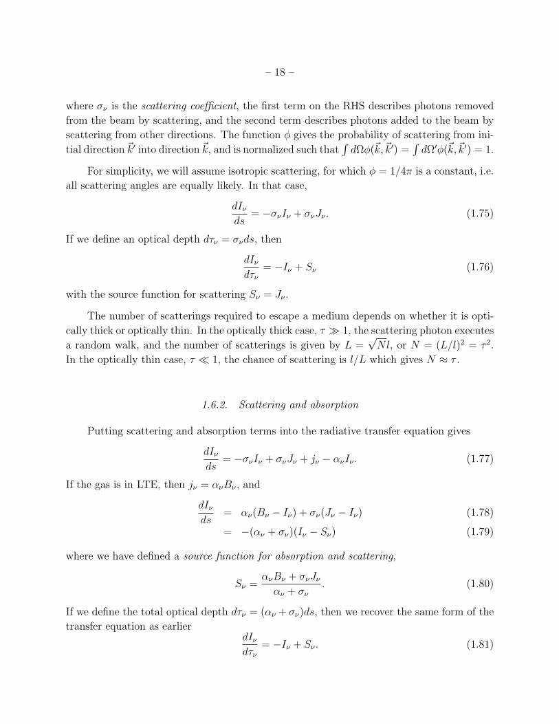
– 17 –

To get some intuition for this, a simple problem is a background source viewed through

a layer of gas in LTE at temperature T .

The solution is

I⌫ = I⌫(0)e�⌧⌫ + B⌫(T )(1� e�⌧⌫ ). (1.72)

Now, if I⌫(0) > B⌫(T ) then

I⌫ = [I⌫(0)�B⌫(T )] e�⌧⌫ + B⌫(T ) (1.73)

is smaller at larger ⌧ , and so would give absorption lines at frequencies where ↵⌫ is larger

than the continuum absorption coe�cient. (See also problem 1.9 in Rybicki and Lightman).

If I⌫(0) < B⌫(T ) on the other hand (e.g. the source is cooler than the layer of gas), then

the brightness will be larger at frequencies with a higher optical depth, and an emission line

spectrum would be seen.

1.6. Scattering

So far, we have not included scattering processes. The reason is that in general including

scattering introduces significant complexity in solving the equation of radiative transfer.

Scattering abruptly changes the direction and possibly frequency of the scattered photon,

resulting in an integro-di↵erential equation as we will see below.

1.6.1. Scattering only

Start by considering a medium with no emission or absorption, scattering only. We will

assume that the scattering is monochromatic, coherent, elastic – i.e. no change in photon

frequency occurs on scattering, only direction. In general, we can write

dI⌫(~k)

ds= ��⌫I⌫(~k) + �⌫

Z�⌫

⇣~k,~k0

⌘I⌫

⇣~k0⌘

d⌦0 (1.74)

– 18 –

where �⌫ is the scattering coe�cient, the first term on the RHS describes photons removed

from the beam by scattering, and the second term describes photons added to the beam by

scattering from other directions. The function � gives the probability of scattering from ini-

tial direction ~k0 into direction ~k, and is normalized such thatR

d⌦�(~k,~k0) =R

d⌦0�(~k,~k0) = 1.

For simplicity, we will assume isotropic scattering, for which � = 1/4⇡ is a constant, i.e.

all scattering angles are equally likely. In that case,

dI⌫

ds= ��⌫I⌫ + �⌫J⌫ . (1.75)

If we define an optical depth d⌧⌫ = �⌫ds, then

dI⌫

d⌧⌫= �I⌫ + S⌫ (1.76)

with the source function for scattering S⌫ = J⌫ .

The number of scatterings required to escape a medium depends on whether it is opti-

cally thick or optically thin. In the optically thick case, ⌧ � 1, the scattering photon executes

a random walk, and the number of scatterings is given by L =p

Nl, or N = (L/l)2 = ⌧ 2.

In the optically thin case, ⌧ ⌧ 1, the chance of scattering is l/L which gives N ⇡ ⌧ .

1.6.2. Scattering and absorption

Putting scattering and absorption terms into the radiative transfer equation gives

dI⌫

ds= ��⌫I⌫ + �⌫J⌫ + j⌫ � ↵⌫I⌫ . (1.77)

If the gas is in LTE, then j⌫ = ↵⌫B⌫ , and

dI⌫

ds= ↵⌫(B⌫ � I⌫) + �⌫(J⌫ � I⌫) (1.78)

= �(↵⌫ + �⌫)(I⌫ � S⌫) (1.79)

where we have defined a source function for absorption and scattering,

S⌫ =↵⌫B⌫ + �⌫J⌫

↵⌫ + �⌫

. (1.80)

If we define the total optical depth d⌧⌫ = (↵⌫ + �⌫)ds, then we recover the same form of the

transfer equation as earlierdI⌫

d⌧⌫= �I⌫ + S⌫ . (1.81)

– 19 –

We can check the limits of this expression: if J⌫ ⇡ B⌫ then S⌫ ⇡ B⌫ ; if J⌫ ⇡ 0 then

S⌫ ⇡ B⌫↵⌫/(↵⌫ + �⌫) < B⌫ .

Another way to write the source function is to define the absorption probability ✏⌫ =

↵⌫/(↵⌫ + �⌫). The source function is then S⌫ = ✏⌫B⌫ + (1� ✏⌫)J⌫ .

Now think about the random walk of a photon in a gas with scattering and absorption.

The number of steps before being absorbed is 1/✏⌫ , giving the mean free path to absorption

l? =p

Nl = l/p

✏⌫ . But l = 1/(↵⌫ + �⌫), and so

l? =1p

↵⌫(↵⌫ + �⌫). (1.82)

This length is known as the di↵usion length, thermalization length, or the e↵ective mean free

path. The e↵ective optical thickness is ⌧? = L/l? =p

✏⌧ . When ⌧? ⌧ 1, most photons escape

without being absorbed (but they might scatter multiple times depending on the value of

⌧). This implies a luminosity L = 4⇡↵⌫B⌫V where V is the volume. For ⌧? � 1, we expect

I⌫ ! B⌫ and S⌫ ! B⌫ , giving a luminosity L ⇡ 4⇡↵⌫B⌫(Al?) where Al? is the volume from

which photons can escape, or since ↵⌫l? =p

✏⌫ , we get L ⇡ 4⇡p

✏⌫B⌫A. For ✏⌫ = 1, we

should get L = ⇡B⌫A, so this estimate is o↵ by a factor of 4, but the important point is

that we see that when scattering is included, the emissivity is reduced by a factor ofp

✏⌫ .

There are two competing e↵ects. First, the emitting volume near the surface is increased by

scattering, since the depth from which photons escape is l/p

✏. However, the mean free path

l is shorter by a factor of ✏, so the overall emitting volume is actually smaller byp

✏.

Summary and Further Reading

Here are the main ideas and results that we covered in this part of the course:

• Specific intensity I⌫ and its moments F⌫ , P⌫ , U⌫ = 4⇡J⌫/c. Source function, S⌫ =

j⌫/↵⌫ . Outwards flux F⌫ = ⇡I⌫ for isotropic I⌫ . Closure relations: P⌫ = U⌫/3,

P⌫ = U⌫ .

• Mean free path l = 1/↵ = 1/n� = 1/⇢. Optical depth.

• Radiative transfer equationdI⌫

ds= j⌫ � ↵⌫I⌫

• General solution. For constant source function,

I⌫ = I⌫(0)e�⌧⌫ + S⌫

�1� e�⌧⌫

�,

– 20 –

giving I⌫ ! S⌫ for ⌧ � 1 and I⌫ ⇡ I⌫(0) + ⌧S⌫ for ⌧ ⌧ 1.

• Thermal radiation. U = aT 4, P = (1/3)aT 4. Properties of Planck spectrum. �max

=

0.29 cm/T . Kircho↵’s Law j⌫ = ↵⌫B⌫ .

• Local thermodynamic equilibrium (LTE). Radiative di↵usion equation. Rosseland

mean opacity.

• Stellar atmospheres. The Eddington approximation and the source function and tem-

perature profile of a grey atmosphere. ⌧ = 2/3 as the photosphere. Limb darkening.

• Emission lines from optically thin thermal gas. Conditions for forming absorption lines.

• Scattering as a random walk. Number of scatterings to escape max(⌧, ⌧ 2). Source

function

S⌫ =↵⌫B⌫ + �⌫J⌫

↵⌫ + �⌫

= ✏⌫B⌫ + (1� ✏⌫)J⌫ .

Thermalization depth. Emissivity of a scattering atmosphere F⌫ =p

✏⌫⇡B⌫ .

Reading

• Rybicki and Lightman, chapter 1.

• Chandrasekhar, S. “Radiative Transfer” Dover 1960. Classic treatise on radiative trans-

fer. Analytic solution for grey atmosphere.

• Mihalas, D. “Stellar atmospheres” W.H. Freeman & Co. 1978. Now unfortunately out

of print. Detailed treatment of the physics of atmospheres and also it tells you how to

calculate a “real” stellar atmosphere.

Appendix: Chandra’s exact solution for a grey atmosphere

In his book Radiative Transfer, Chandrasekhar presents a beautiful analytic solution

to the grey atmosphere. We summarize it here, and compare the results with our solution

derived using the Eddington approximation.

For a grey atmosphere, S = J regardless of the degree of scattering or absorption. The

transfer equation is

µdI

d⌧(⌧, µ) = I (⌧, µ)�

1

2

Z1

�1

dµ0I (⌧, µ0) (1.83)

– 21 –

an integral equation for I(⌧, µ).

If we follow only a finite set of µ values, the integral can be written as a sum,

µidIi

d⌧= Ii �

1

2

XajIj (1.84)

for i = ±1,±2,...±n. Gaussian quadrature is used to choose the appropriate µi’s and the

corresponding ai’s. For Z1

�1

f(µ)dµ =mX

j=1

ajf(µj) (1.85)

the appropriate choice is to choose the µi to be the zeroes of Pm(µ), and

aj =1

P 0m(µj)

Z1

�1

dµPm(µ)

µ� µj

(1.86)

(wherePm

j=1

aj = 1) (e.g. see Chandra’s book or numerical recipes). This choice gives an

exact solution for f(µ) a polynomial with order < 2m. For integrals of the formR

e�xf(x)dx,

the Laguerre polynomials are used instead. For any weight function (e�x in this case), a set of

µi and ai can be constructed that solves the integral exactly for f(x) a polynomial of degree

< 2m. This is therefore a good technique for numerically integrating smooth functions. Note

that Chandra uses the terminology “nth approximation” for m = 2n, i.e. we use the roots

of P2n(µ) for which aj = a�j and µ�j = �µj.

Chandra derived an analytic solution for equation (1.84). First, we look for a solution

with exponential dependence on ⌧ , Ii = gie�k⌧ , i = ±1,...±n. Substituting this into equation

(1.84) gives

gi =constant

1 + µik(1.87)

where k is determined by

1 =nX

j=1

aj

1� µ2

jk2

. (1.88)

There are 2n�2 roots ±k↵, for ↵ = 1,...n�1. We keep only the k > 0 roots, since we want I

finite at large optical depth. There is also a solution linear in ⌧ , Ii = b(⌧ + qi), i = ±1,...±n.

Substituting into equation (1.84) gives qi = Q + µi where Q is a constant. Therefore, the

solution is

Ii = b

"n�1X

↵=1

L↵e�k↵⌧

1 + µik↵

+ ⌧ + µi + Q

#(1.89)

which has n constants Q and L↵ to be determined. To fix their values, we set I�i = 0 at

⌧ = 0 (no ingoing radiation at the surface) which givesn�1X

↵=1

L↵

1� µik↵

� µi + Q = 0 i = 1, ...n (1.90)

– 22 –

Given the analytic expression for Ii, the flux, pressure and mean intensity can be cal-

culated

F = 2⇡X

aiµiIi (1.91)

cP

4⇡= K =

1

2

Xaiµ

2

i Ii =F

4⇡(⌧ + Q) (1.92)

J =1

2

XaiIi =

3F

4⇡[⌧ + q(⌧)] (1.93)

where

q(⌧) = Q +n�1X

↵=1

L↵e�k↵⌧ . (1.94)

Putting S = J , we can then solve for I(µ) for all values of µ,

I(⌧, +µ) =3F

4⇡

"n�1X

↵=1

L↵e�k↵⌧

1 + k↵µ+ ⌧ + µ + Q

#(1.95)

and at the surface

I(µ) =3F

4⇡

"n�1X

↵=1

L↵

1 + k↵µ+ µ + Q

#=

3F

4⇡

H(µ)p

3. (1.96)

The tables in Chandra’s book give Q, L↵, and k↵ for di↵erent n’s. At all orders, the Hopf-

Bronstein relation holds at ⌧ = 0, J(0) =p

3F/4⇡.

To make a connection with our Eddington approximation solution, let’s look at the first

approximation (n = 1). Then looking at Chandra’s table VIII we find Q = 1/p

3, and we

have two photon directions µ± = ±1/p

3 which are the roots of P2

(µ) (there are no L↵’s

to consider for n = 1). This gives another way to understand the discussion in Rybicki

and Lightman section 1.10, where they introduce a “two stream approximation” using these

angles, motivating them by saying that this choice gives moments that satisfy the Eddington

approximation. Another point to note is that this solution is very similar to the Eddington

approximation solution, but with Q = 1/p

3 = 0.58 rather than Q = 2/3 = 0.67. The

di↵erent approximations made in each case are that in Chandra’s solution, the ratio 3P/U

is not assumed to be constant, but only two photon directions are followed, whereas in the

Eddington approximation the ratio 3P/U is fixed to be unity, but all photon angles are

followed.

Let’s check the limb darkening ratio. For the Eddington approximation, this was I(µ =

0)/I(µ = 1) = 2/5. In the first approximation I(µ = 0)/I(µ = 1) = Q/(1+Q) = 0.37. In the

second approximation n = 2, we have Q = 0.694, k1

= 1.97, and L1

= �0.117. The angles are

– 23 –

µ±1

= ±0.340 and µ±2

= ±0.861. Then I(µ = 0)/I(µ = 1) = (Q+L1

)/(1+Q+L1

/(1+k1

)) =

0.35.

Next, look at the temperature profile which is given by equation (1.93) with J = S = B.

Then

T 4 =3

4T 4

e↵

(⌧ + q(⌧)) . (1.97)

In the Eddington approximation, q(⌧) = 2/3. In the first approximation n = 1, we have

q(⌧) = 1/p

3. In the second approximation,

q(⌧) = Q + L1

e�k1

⌧ (1.98)

which changes from Q + L1

= 0.577 at ⌧ = 0 to Q = 0.694 at large ⌧ .

– 24 –

2. Radiation from Accelerating Charges

These are notes for part two of PHYS 642 Radiative Processes in Astrophysics. The

basic physics underlying the radiation that we see is that accelerating charges radiate. The

power radiated from a single charged particle q moving non-relativistically (u ⌧ c) is given

by Larmor’s formula

P =2q2u2

3c3

(2.1)

where u is the magnitude of the acceleration. In this section, we derive this equation, and

use it to understand the emission from a thermal plasma due to scattering of electrons from

ions, bremstrahlung radiation. Next , we consider emission from collections of particles using

the multipole expansion. Applications include: X-ray emission from galaxy clusters, free-free

opacity in stars, the spectra of compact HII regions, emission from spinning dust, and the

spin down of radio pulsars.

2.1. Derivation of the radiation field of an accelerated charge

Here we go through the derivation of the radiation fields of an accelerating charge

starting with Maxwell’s equations. We’ll skip a lot of the algebra and focus on the physical

ideas.

In cgs units, Maxwell’s equations are

~r ·

~E = 4⇡⇢ (2.2)

~r⇥

~B =4⇡ ~J

c+

1

c

@ ~E

@t(2.3)

~r⇥

~E = �

1

c

@ ~B

@t(2.4)

~r ·

~B = 0 (2.5)

together with charge conservation

@⇢

@t+ ~r ·

~J = 0. (2.6)

In these units, the Lorentz force is

~F = q

~E +

~v ⇥ ~B

c

!. (2.7)

– 25 –

It is convenient to work with potentials

~r⇥

~A = ~B ~E = �~r��1

c

@ ~A

@t(2.8)

(recall that the ~B field is always divergence free, but ~E can have both divergence and curl if

@ ~B/@t is non-zero).

Substituting these potentials into Maxwell’s equations gives

r

2 ~A�1

c2

@2 ~A

@t2= �

4⇡ ~J

c+ ~r

~r ·

~A +1

c

@�

@t

�(2.9)

r

2��1

c2

@2�

@t2= 4⇡⇢+

1

c

@

@t

~r ·

~A +1

c

@�

@t

�. (2.10)

I’ve written the equations this way to emphasize that � and ~A satisfy the inhomogeneous

wave equation

r

2

⇣~A,�⌘�

1

c2

@2

@t2

⇣~A,�⌘

= 4⇡

�

~J

c, ⇢

!(2.11)

if we choose~r ·

~A +1

c

@�

@t= 0. (2.12)

In fact we are free to choose ~r ·

~A (only the curl of ~A which gives ~B is the physical quantity)

in this way – this choice is the Lorenz gauge.

The solutions to equations (2.11) are the retarded potentials

�(~r, t) =

Z ⇢⇣~r0, t0

⌘d3~r0

���~r � ~r0���

(2.13)

~A(~r, t) =1

c

Z ~J⇣~r0, t0

⌘d3~r0

���~r � ~r0���

(2.14)

where the integrand is evaluated at the retarded time

t0 = t�

���~r � ~r0���

c. (2.15)

The physics of this makes sense – the relevant value of the source (⇢ or ~J) is the value a light

travel time ago. Electromagnetic disturbances propagate at the speed of light. In electro- or

magnetostatics, t0 ! t, and the expressions for the potentials should be familiar.

– 26 –

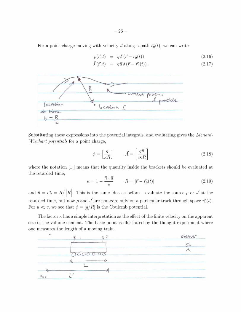
For a point charge moving with velocity ~u along a path ~r0

(t), we can write

⇢(~r, t) = q � (~r � ~r0

(t)) (2.16)~J (~r, t) = q~u � (~r � ~r

0

(t)) . (2.17)

Substituting these expressions into the potential integrals, and evaluating gives the Lienard-

Wiechart potentials for a point charge,

� =h q

R

i~A =

q~u

cR

�(2.18)

where the notation [...] means that the quantity inside the brackets should be evaluated at

the retarded time,

= 1�~n · ~u

cR = |~r � ~r

0

(t)| (2.19)

and ~n = ~eR = ~R/���~R���. This is the same idea as before – evaluate the source ⇢ or ~J at the

retarded time, but now ⇢ and ~J are non-zero only on a particular track through space ~r0

(t).

For u⌧ c, we see that � = [q/R] is the Coulomb potential.

The factor has a simple interpretation as the e↵ect of the finite velocity on the apparent

size of the volume element. The basic point is illustrated by the thought experiment where

one measures the length of a moving train.

– 27 –

Photon 1 is emitted from the far side of the train at t = 0. It is straightforward to show that

photon 2 from the front of the train should be emitted at position x = L0 if it is to arrive at

the observer at the same time as photon 1, where

L0 =L

1� v/c. (2.20)

The length L0 is the apparent length of the train. The volume element d3~r0 in the integral

undergoes the same distortionZ⇢d3~r0 =

q

1� ~n · ~u/c. (2.21)

We think the charge is spread out over a larger volume than it actually is.

Once we know the potentials, we can di↵erentiate to find the fields. This is where we

skip some algebra, and give the result,

~E(~r, t) =h q

3R2

⇣~n� ~�

⌘ �1� �2

�i+

"q

3Rc~n⇥

(⇣~n� ~�

⌘⇥

@~�

@t

)#(2.22)

~B(~r, t) =h~n⇥ ~E

i, (2.23)

where ~� = ~u/c.

Let’s take a closer look at each term and see if they make sense. The first term is known

as the velocity field,~EV =

h q

3R2

⇣~n� ~�

⌘ �1� �2

�i. (2.24)

For � ⌧ 1, ~EV = [q~n/R2] which is Coulomb’s law, and ~B is smaller by � than ~E. The vector

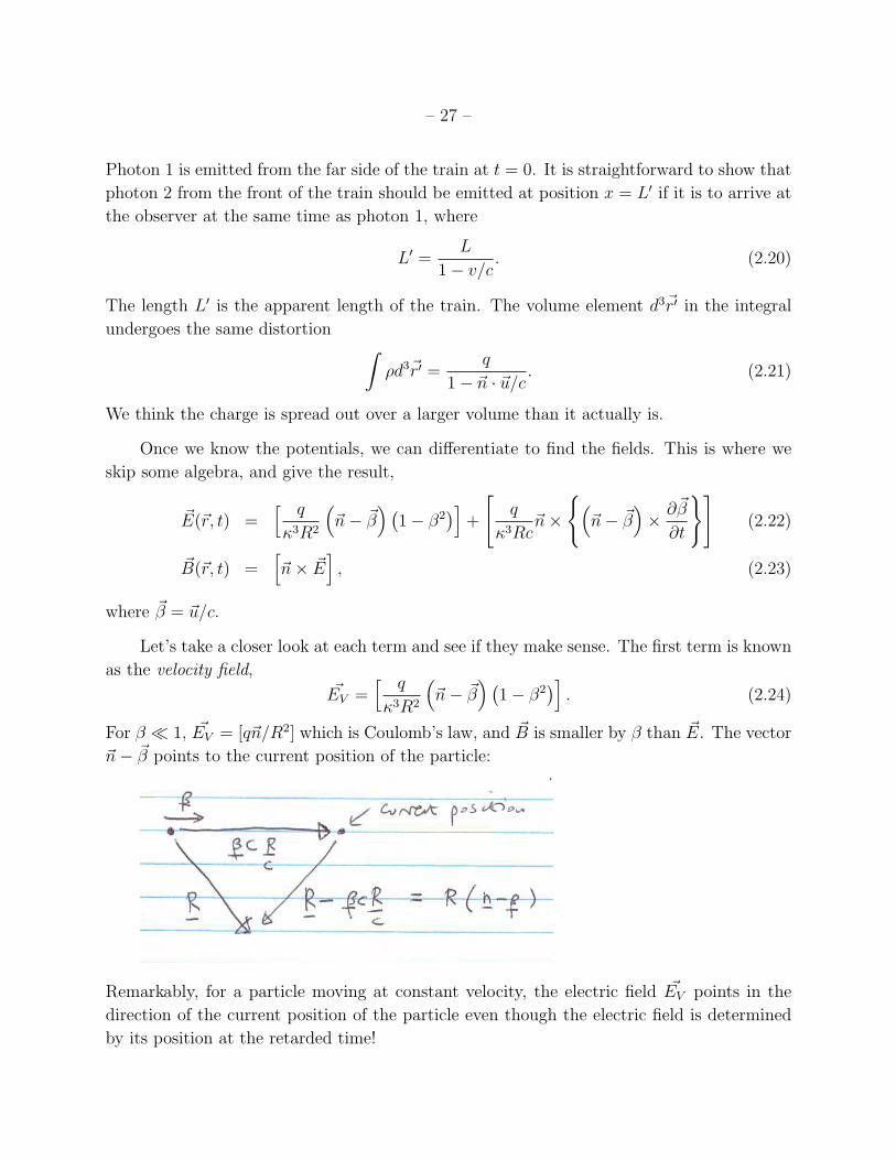
~n� ~� points to the current position of the particle:

Remarkably, for a particle moving at constant velocity, the electric field ~EV points in the

direction of the current position of the particle even though the electric field is determined

by its position at the retarded time!

– 28 –

The second term, which involves @~�/@t, is called the acceleration field or radiation field,

~Erad

=

"q

3Rc~n⇥

(⇣~n� ~�

⌘⇥

@~�

@t

)#. (2.25)

This is the term that gives rise to radiation. Since Erad

/ 1/R, the Poynting flux is / 1/R2,

giving a constant energy per unit area at large distance since the area of constant solid angle

increases / R2. The velocity field decreases as 1/R2 (as for the static Coulomb field), and

does not therefore contribute at large R.

2.2. Radiation from non-relativistic particles: Larmor’s formula

We will need the relativistic version of ~Erad

later for emission by relativistic particles,

but for now we assume � ⌧ 1, and therefore = 1, and we need not distinguish between

the current time and the retarded time. Our aim is to calculate the Poynting flux

~S =c

4⇡~E ⇥ ~B. (2.26)

Since ~B = ~n⇥ ~E, then

~S =c

4⇡

⇣~E ⇥

⇣~n⇥ ~E

⌘⌘=

c

4⇡~n��� ~E���2

(2.27)

where we use the fact that ~n ·

~E = 0.

Now substitute

~Erad

⇡

q

Rc~n⇥

~n⇥

@~�

@t

!(2.28)

gives

~S = ~nq2

4⇡c3R2

���~n⇥⇣~n⇥ ~u

⌘���2

. (2.29)

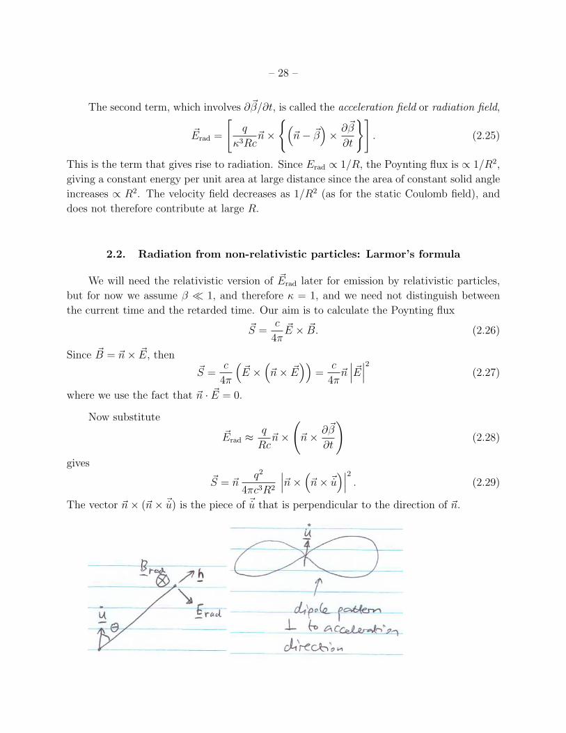
The vector ~n⇥ (~n⇥ ~u) is the piece of ~u that is perpendicular to the direction of ~n.

– 29 –

Therefore we see that the radiation electric field is perpendicular to the radial direction,

which is why it leads to a radial Poynting flux.

Defining the angle ⇥ so that���~n⇥ (~n⇥ ~u)

���2

= sin2 ⇥, we arrive at the final result

~S = ~nq2u2

4⇡R2c3

sin2 ⇥, (2.30)

which is the flux at distance R and angle ⇥. Now since the area element is dA = R2d⌦, then

we can rewrite this asdW

dtd⌦=

q2u2

4⇡c3

sin2 ⇥, (2.31)

which is the power radiated per unit solid angle at angle ⇥.

The total power radiated is given by integrating over all solid angles

P =dW

dt=

(qu)2

4⇡c3

Zsin ⇥2d⌦ (2.32)

or

P =2q2u2

3c3

, (2.33)

which is Larmor’s formula.

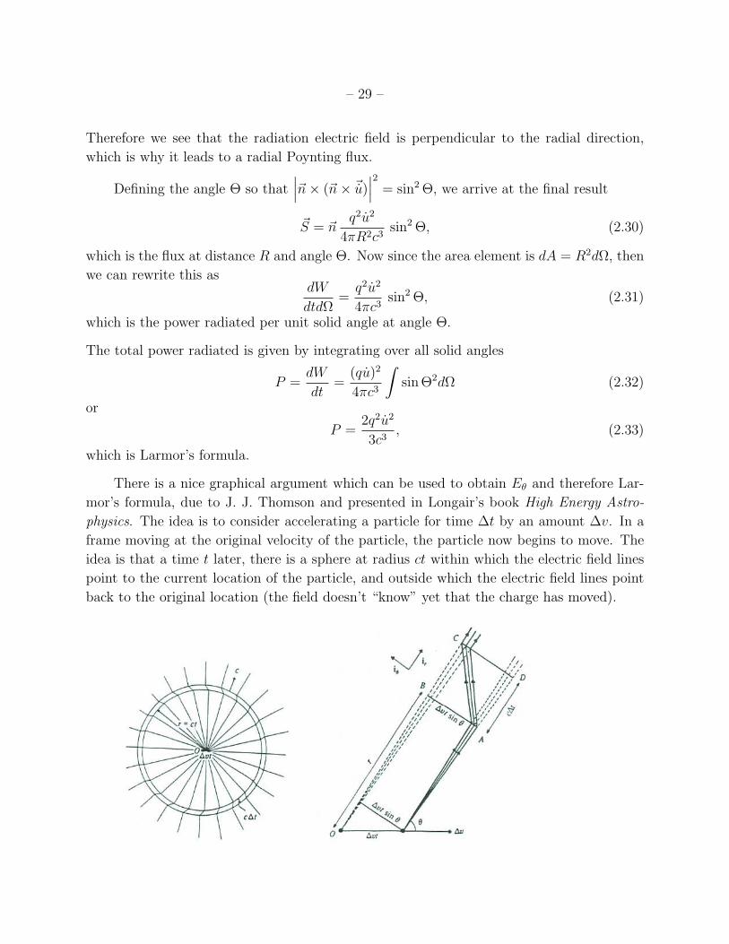
There is a nice graphical argument which can be used to obtain E✓ and therefore Lar-

mor’s formula, due to J. J. Thomson and presented in Longair’s book High Energy Astro-

physics. The idea is to consider accelerating a particle for time �t by an amount �v. In a

frame moving at the original velocity of the particle, the particle now begins to move. The

idea is that a time t later, there is a sphere at radius ct within which the electric field lines

point to the current location of the particle, and outside which the electric field lines point

back to the original location (the field doesn’t “know” yet that the charge has moved).

– 30 –

The Figures you need are above, taken from Longair. The graphical argument gives

E✓

Er

=(�v)t sin ✓

c�t(2.34)

but Er = q/r2 = q/(ct)2, and so E✓ = qu sin ✓/c2r, exactly as we found earlier. This shows

very nicely that E✓/Er grows with time t / r, and so E✓ / 1/r.

2.3. The spectrum of the emitted radiation

Next, we consider the frequency spectrum of the radiation. As might be expected, the

frequency spectrum is related to the time history of the acceleration of the particle. To see

this, we write the power radiated per unit solid angle as

dW

dtd⌦=

c

4⇡

���R ~E���2

=��� ~A(t)

���2

(2.35)

(note that ~A is not the vector potential, but a temporary definition for this section; we are

following the notation and argument of Jackson 14.5). The argument is to integrate over all

time to get the total energy emitted per unit solid angle,

dW

d⌦=

Z 1

�1

��� ~A(t)���2

dt =

Z 1

�1

��� ~A(!)���2

d! (2.36)

where Parseval’s theorem has been used to rewrite the integral in terms of the Fourier

transform of ~A(t). We write the Fourier transforms as6

~A(t) =1p

2⇡

Z 1

�1

~A(!)e�i!td! ~A(!) =1p

2⇡

Z 1

�1

~A(t)ei!tdt. (2.37)

If ~A(t) is real, then ~A(�!) = ~A⇤(!), and so we can integrate over positive frequencies over

and multiply by two. The energy radiated per unit solid angle per unit frequency interval is

thereforedW

d!d⌦= 2

��� ~A(!)���2

. (2.38)

6As usual, beware of di↵erent normalizations used by di↵erent authors. I prefer the symmetry of putting1/p

2⇡ in front of each integral in the pair; Rybicki and Lightman put the full 1/2⇡ in front of the integralfor ~A(!).

– 31 –

2.4. Thermal Bremsstrahlung

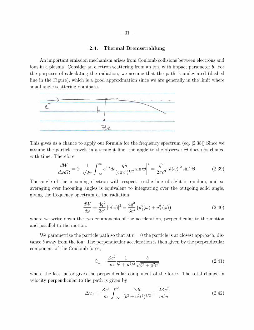
An important emission mechanism arises from Coulomb collisions between electrons and

ions in a plasma. Consider an electron scattering from an ion, with impact parameter b. For

the purposes of calculating the radiation, we assume that the path is undeviated (dashed

line in the Figure), which is a good approximation since we are generally in the limit where

small angle scattering dominates.

This gives us a chance to apply our formula for the frequency spectrum (eq. [2.38]) Since we

assume the particle travels in a straight line, the angle to the observer ⇥ does not change

with time. Therefore

dW

d!d⌦= 2

����1p

2⇡

Z 1

�1ei!tdt

qu

(4⇡c3)1/2

sin ⇥

����2

=q2

2⇡c3

|u(!)|2 sin2 ⇥. (2.39)

The angle of the incoming electron with respect to the line of sight is random, and so

averaging over incoming angles is equivalent to integrating over the outgoing solid angle,

giving the frequency spectrum of the radiation

dW

d!=

4q2

3c3

|u(!)|2 =4q2

3c3

�u2

k(!) + u2

?(!)�

(2.40)

where we write down the two components of the acceleration, perpendicular to the motion

and parallel to the motion.

We parametrize the particle path so that at t = 0 the particle is at closest approach, dis-

tance b away from the ion. The perpendicular acceleration is then given by the perpendicular

component of the Coulomb force,

u? =Ze2

m

1

b2 + u2t2b

p

b2 + u2t2(2.41)

where the last factor gives the perpendicular component of the force. The total change in

velocity perpendicular to the path is given by

�u? =Ze2

m

Z 1

�1

b dt

(b2 + u2t2)3/2

=2Ze2

mbu(2.42)

– 32 –

It is straightforward to see that this is much larger than the acceleration parallel to the

path. Energy conservation gives before and after scattering u2 = (u � �uk)2 + �u2

?, or

�uk/�u? ⇡ Ze2/bmu2 which is small for small angle collisions.

Therefore,

u(!) =1p

2⇡

Z 1

�1ei!tdt

Ze2

m

b

(b2 + u2t2)3/2

(2.43)

=1p

2⇡

Ze2

mub

Z 1

�1

dx eix!b/u

(1 + x2)3/2

=

r2

⇡

Ze2

mubyK

1

(y) (2.44)

where y = !b/u and K1

(y) is a modified Bessel function. The limits are yK1

(y) ⇡ 1 for

low frequencies ! ⌧ v/b, and yK1

(y) ⇡ (y⇡/2)1/2e�y for ! � v/b. That is the frequency

spectrum is constant below ! = u/b, and falls to zero for higher frequencies. This makes

sense because since b is the distance of closest approach, b/v is the shortest timescale in the

problem, and we might expect no higher frequency components. On the other hand, at low

frequencies, the ei!t term is approximately unity, and u(!) ⇡ �u/p

2⇡. Another way to look

at it is that the interaction is strongly peaked around t = 0 when the particle is at closest

approach, and therefore the frequency spectrum is very broad.

Substituting u?(!) into equation (2.40) gives the spectrum for a single particle collision

averaged over angles for a particle value of impact parameter b. The total emission rate per

unit volume is

dW

dt d! dV= nineu

Z bmax

bmin

2⇡b dbdW

d!(b) (2.45)

=16Z2e6

3m2c3uneni

Z bmax

bmin

db

b

✓!b

u

◆K

1

✓!b

u

◆�2

(2.46)

An approximate way to write this is

dW

dt d! dV=

16Z2e6

3m2c3uneni

Z bmax

bmin

db

b(2.47)

for !b/u < 1, and zero for !b/u > 1. The integral over impact parameters gives the Coulomb

logarithm

⇤ = ln

✓bmax

bmin

◆, (2.48)

which indicates a logarithmic divergence for large bmax

that arises because the Coulomb force

is a long range force.

How do we choose bmax

? To be consistent with our approximation for the integral, we

should choose bmax

= u/!, that is only consider values of b that give a contribution to the

– 33 –

spectrum at frequency !. For bmin

there are two possibilities. The “classical” approach is to

choose bmin

as the impact parameter where �u? = u, that is the impact parameter where

a large angle scatter occurs, giving bmin

= 2Ze2/mu2. (This is also the distance of closest

approach for a repulsive interaction.) However, if bmin

= ~/meu is larger, then we should

choose that instead. Then quantum mechanics sets bmin

. You can think of this as the impact

parameter of a particle with one quantum of angular momentum. The changeover occurs

when 2Ze2/mu2 = ~/mu or

1

2mu2 = Z2

✓e2

~c

◆2

mc2 = Z2↵2mc2 = Z2(13.6 eV) (2.49)

(where ↵ = e2/~c is the fine structure constant). We see that the classical calculation is no

longer appropriate when the electron energy exceeds Z2Ry.

In general, the emissivity is written as

dW

dt d! dV=

16e6

3m2c3uneniZ

2

⇡p

3gff

�(2.50)

where gff (!, u) is the Gaunt factor. As our classical calculation indicated, the Gaunt factor

is typically a slowly varying function of ! and u, so that the prefactor gives the major

dependence. A classic paper which presents calculations of gff is Karzas and Latter (1961).

The Gaunt factor is also plotted in Rybicki and Lightman’s book. You’ll see the parameter

� = Z2Ry/kBT which measures the transition between the classical and quantum regimes.

For a gas with a thermal distribution of velocities,

f(u)du =

✓m

2⇡kBT

◆3/2

exp

✓�

mu2

2kBT

◆4⇡u2du (2.51)

we can average over the velocity distribution to obtain the total emissivity due to ther-

mal bremsstrahlung. However, we must be careful to cut o↵ the velocity distribution at a

minimum velocity umin

where ~! = mu2

min

/2. This accounts for photon discreteness, that

is the incoming electron must have enough energy to produce the photon of frequency !.

Combining equations (2.50) and (2.51), we can see that the answer will look like

dW

dtdV d!/

Z 1

umin

u2du exp

✓�

mu2

2kBT

◆gff (u)

u(2.52)

/ gff

Z 1

u2

min

d(u2) exp

✓�

mu2

2kBT

◆(2.53)

/ gff exp

✓�

~!kBT

◆(2.54)

– 34 –

for a suitably averaged Gaunt factor gff . Keeping the prefactors, the result is

dW

dtdV d!=

25⇡e6

3mc3

✓2⇡

3kBm

◆1/2

Z2T�1/2nenie�~!/kBT gff (2.55)

or

✏ff⌫ = 6.8⇥ 10�38 erg s�1 cm�3 Hz�1 Z2neniT

�1/2e�h⌫/kBT gff (2.56)

where gff is the thermally-averaged Gaunt factor, ✏⌫ is the emissivity (where j⌫ = ✏⌫/4⇡).

We write “↵” for “free-free” which refers to the fact that we can think of the electron as

making a transition between states in the continuum.

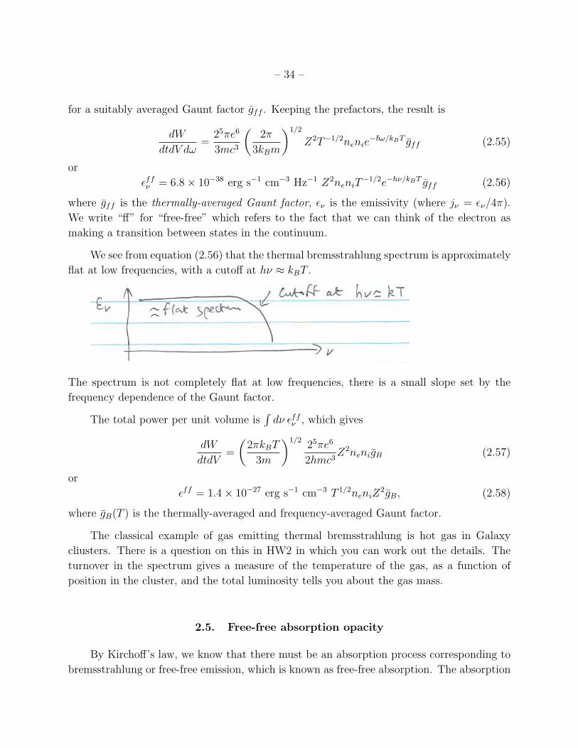
We see from equation (2.56) that the thermal bremsstrahlung spectrum is approximately

flat at low frequencies, with a cuto↵ at h⌫ ⇡ kBT .

The spectrum is not completely flat at low frequencies, there is a small slope set by the

frequency dependence of the Gaunt factor.

The total power per unit volume isR

d⌫ ✏ff⌫ , which gives

dW

dtdV=

✓2⇡kBT

3m

◆1/2 25⇡e6

2hmc3

Z2nenigB (2.57)

or

✏ff = 1.4⇥ 10�27 erg s�1 cm�3 T 1/2neniZ2gB, (2.58)

where gB(T ) is the thermally-averaged and frequency-averaged Gaunt factor.

The classical example of gas emitting thermal bremsstrahlung is hot gas in Galaxy

cliusters. There is a question on this in HW2 in which you can work out the details. The

turnover in the spectrum gives a measure of the temperature of the gas, as a function of

position in the cluster, and the total luminosity tells you about the gas mass.

2.5. Free-free absorption opacity

By Kircho↵’s law, we know that there must be an absorption process corresponding to

bremsstrahlung or free-free emission, which is known as free-free absorption. The absorption

– 35 –

coe�cient is given by

↵ff⌫ =

jff⌫

B⌫(T )=

1

4⇡B⌫(T )

dW

dtdV d⌫(2.59)

=4e6

3mch

✓2⇡

3kBm

◆1/2

T�1/2Z2neni⌫�3

�1� e�h⌫/kBT

�gff (2.60)

= 3.7⇥ 108 cm�1 T�1/2Z2neni⌫�3

�1� e�h⌫/kBT

�gff . (2.61)

In the Rayleigh-Jeans limit, h⌫ ⌧ kBT , ↵ff⌫ = 0.018 cm�1 T�3/2Z2neni⌫

�2gff .

In optically thick regions, the Rosseland mean opacity is the relevant quantity. Recall

that the Rosseland mean is defined byZ

d⌫dB⌫

dT

�1

↵R

=

Zd⌫

1

↵⌫

dB⌫

dT

�. (2.62)

The result is

↵ffR = 1.7⇥ 10�25 T�7/2Z2nenigR, (2.63)

where the prefactor comes from Rybicki and Lightman. The T�7/2 factor comes from the

T�1/2⌫�3 dependence of the frequency-dependent opacity, since the averaging replaces h⌫

with a multiple of kBT . For use in stellar interiors, it is more convenient to write down an

expression for the opacity R = ↵R/⇢. To do so, we write ne = ⇢Ye/mp, where Ye is the

number fraction of electrons, and ni = ⇢Yi/mp where Yi is the number fraction of nuclei.

The opacity is then

ffR = 6.1⇥ 1022 cm2 g�1

⇢Ye

T 7/2

gR

X

i

XiZ2

i

Ai

, (2.64)

where the sum is over the charges Zi, masses Ai, and mass fractions Xi of nuclei. In terms of

the nuclear charges and masses, Ye =P

i XiZi/Ai and Yi =P

i Xi/Ai. **The prefactor here

doesn’t agree with Clayton or Itoh who have 7.53⇥ 1022**. The result / ⇢T�7/2 is known

as Kramer’s law. A rough rule is that free-free absorption is important in stars less massive

than the Sun, and Thomson scattering in stars more massive than the Sun. This is shown

in HW2, where you will see that it results in a change in the slope of the luminosity-mass

relation for main sequence stars at around 1 M�.

Another application to mention is to compact HII regions, which can be optically thick

to free-free absorption at low frequencies (↵ff⌫ / ⌫�2 at low frequencies). They are said to

be self-absorbed and this gives a falling spectrum at low frequencies, as you will see in HW

2.

– 36 –

2.6. Multipole radiation

So far we have dicussed radiation resulting from acceleration of a single particle. We

now turn to a collection of particles, and use the multipole expansion to evaluate the radiated

power.

First, a reminder of the multipole expansion in electrostatics or magnetostatics. The

electrostatic potential at a large distance from a charge distribution can be expanded as

�(~r) =

Z⇢(~r0)d3~r0���~r � ~r0

���=

Q

r+~er · ~p

r2

+~er · Q2 · ~er

r3

+ ... (2.65)

where

Q =

Z⇢(~r0)d3~r0 (2.66)

is the total charge,

~p =

Z⇢(~r0)~r0d3~r0 (2.67)

is the electric dipole moment, and

(Q2)ij =

Z⇢(~r0)

⇥3r0ir

0j � r02�ij

⇤d3~r0 (2.68)

is the electric quadrupole moment tensor. Similarly, for a current distribution, the vector

potential can be expanded

~A(~r) =1

c

Z ~J(~r0)d3~r0���~r � ~r0���

=~m⇥ ~er

r2

+ ... (2.69)

where

~m =1

2c

Z~r0 ⇥ ~J(~r0)d3~r0 (2.70)

is the magnetic dipole moment. To derive these results, expand

1���~r � ~r0���⇡

1

r

1 +

~er ·~r0

r+

3(~er ·~r0)2

� r02

r2

+ ...

!. (2.71)

The idea is to now do something similar for the time-dependent case, in particular to

expand the retarded potentials (eqs. [2.13] and [2.14]) and therefore radiation fields as a

sum of multipole components. In the time-dependent case, there is a new lengthscale in the

problem, which is the wavelength of the emitted radiation �. We will assume that the size of

– 37 –

the emitting region d⌧ �⌧ r, and that the particles are non-relativistic. (In other words,

the light-crossing time d/c is much smaller than the wave period 2⇡/! = 2⇡/ck = �/c.)

We start by looking at an individual Fourier components ~J(~r, t) = ~J(~r)e�i!t etc. The

spatial part of the vector potential is then, from equation (2.14),

~A(~r) =1

c

Z~J(~r0)d3~r0

eik|

~r�~r0|

���~r � ~r0���

(2.72)

since the integrand is evaluated at the retarded time (t0 = t����~r � ~r0

��� /c). Our approach will

be to calculate ~A(~r) and then obtain the fields from

~B = ~r⇥

~A ~E =i

k~r⇥

~B (2.73)

(this is simpler than expanding � and using that to obtain ~E). The relation between ~E and~B holds since outside the source there are no currents and @ ~E/@t = c~r⇥ ~B.

2.6.1. Electric dipole

We start with the electric dipole term by writing���~r � ~r0

��� ⇡ r. This means that we

ignore variations in the retarded time across the source. Then

~A(~r) ⇡1

rceikr

Z~J(~r0)d3~r0. (2.74)

To simplify this term, integrate by parts using ~r · (ri

~J) = ri~r ·

~J + ~J ·

~rri = i!⇢ri + Ji.

The surface term vanishes, giving

~A(~r) = �ik

reikr

Z⇢(~r0)~r0d3~r0 = �

ik~peikr

r. (2.75)

The radiation fields are therefore

~B =k2eikr

r~n⇥ ~p (2.76)

~E = ~B ⇥ ~n =k2eikr

r~n⇥ (~p⇥ ~n) . (2.77)

The power radiated is

dP

d⌦=

c

8⇡Rehr2~n ·

~E ⇥ ~B?i

=c

8⇡k4

|~p|2 sin2 ✓ (2.78)

– 38 –

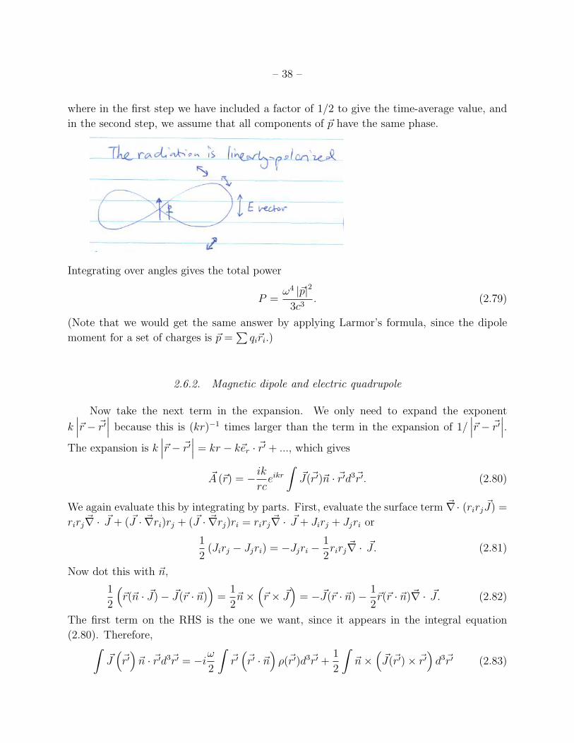
where in the first step we have included a factor of 1/2 to give the time-average value, and

in the second step, we assume that all components of ~p have the same phase.

Integrating over angles gives the total power

P =!4

|~p|2

3c3

. (2.79)

(Note that we would get the same answer by applying Larmor’s formula, since the dipole

moment for a set of charges is ~p =P

qi~ri.)

2.6.2. Magnetic dipole and electric quadrupole

Now take the next term in the expansion. We only need to expand the exponent

k���~r � ~r0

��� because this is (kr)�1 times larger than the term in the expansion of 1/���~r � ~r0

���.

The expansion is k���~r � ~r0

��� = kr � k~er ·~r0 + ..., which gives

~A (~r) = �ik

rceikr

Z~J(~r0)~n ·

~r0d3~r0. (2.80)

We again evaluate this by integrating by parts. First, evaluate the surface term ~r · (rirj

~J) =

rirj~r ·

~J + ( ~J ·

~rri)rj + ( ~J ·

~rrj)ri = rirj

~r ·

~J + Jirj + Jjri or

1

2(Jirj � Jjri) = �Jjri �

1

2rirj

~r ·

~J. (2.81)

Now dot this with ~n,

1

2

⇣~r(~n ·

~J)� ~J(~r · ~n)⌘

=1

2~n⇥

⇣~r ⇥ ~J

⌘= � ~J(~r · ~n)�

1

2~r(~r · ~n)~r ·

~J. (2.82)

The first term on the RHS is the one we want, since it appears in the integral equation

(2.80). Therefore,Z

~J⇣~r0⌘~n ·

~r0d3~r0 = �i!

2

Z~r0⇣~r0 · ~n

⌘⇢(~r0)d3~r0 +

1

2

Z~n⇥

⇣~J(~r0)⇥ ~r0

⌘d3~r0 (2.83)

– 39 –

The two terms on the RHS represent electric quadrupole radiation and magnetic dipole

radiation respectively.

Let’s take the magnetic dipole term first. Its contribution to ~A is

~A(~r) = �ik

rceikr 1

2~n⇥

Z~J(~r0)⇥ ~r0d3~r0 =

ik

reikr~n⇥ ~m (2.84)

which gives the radiation fields

~E = �k2(~n⇥ ~m)eikr

r~B = k2(~n⇥ ~m)⇥ ~n

eikr

r(2.85)

and radiated powerdP

d⌦=

!4

8⇡c3

|~m|

2 sin2 ✓ P =!4

|~m|

2

3c3

, (2.86)

the (time-averaged) power radiated by an oscillating magnetic dipole. Since the magnetic

dipole moment is of order v/c compared to the electric dipole moment, we see that the power

emitted in this term is ⇠ (v/c)2 times the electric dipole emission.

The electric quadrupole contribution to ~A is

~A = �ik

rceikr

✓�

i!

2

◆Z~r0(~r0 · ~n)⇢(~r0)d3~r0. (2.87)

The integral in this expression is the first term of (Q2

)ijnj ⌘~Q(~n). The remaining term

/ �ij vanishes when we take the cross product of ~A with ~k = ~n to find the magnetic field.

Therefore

~B = �ik3

6

eikr

r~n⇥ ~Q(~n). (2.88)

The radiated power is

dP

d⌦=

c

288⇡k6

���(~n⇥ ~Q(~n))⇥ ~n���2

P =ck6

360

X

ij

|(Q2)ij|2

/ !6. (2.89)

The power emitted is a factor of ⇠ (kd)2 smaller than the electric dipole emission.

2.7. Applications of multipole emission

2.7.1. Spinning dust emission

For example, see Draine and Lazarian (1998). In the interstellar medium, dust grains

become charged due to photoionization and collisions. In general, the charge distribution

– 40 –

has a di↵erent center than the mass distribution, which implies a net dipole moment. Small

molecules also have intrinsic dipole moments. If the rotation axis and dipole axis are mis-

aligned by angle ✓, the radiated power is P = (2/3)(!4p2 sin2 ✓/c3) (this is a factor of 2 larger

than eq. [2.79] since for rotation you can think of two components of ~p perpendicular to the

rotation axis that vary).

To estimate the rotation frequency and therefore frequency of the emitted radiation,

we note that for thermal equilibrium we expect (1/2)I!2 = (3/2)kBT , and the simplest

estimate is to assume I = (2/5)Ma2 where M = 4⇡a3⇢/3. Draine and Lazarian (1998)

assume ⇢ = 2 g cm�3. The result is

⌫ = 5.6⇥ 109 Hz⇣ a

10�7 cm

⌘�5/2

✓T

100 K

◆1/2

. (2.90)

Therefore, we expect radiation in the GHz range (wavelengths of ⇡ 10 cm). For estimates of

the dipole moment, see Draine and Lazarian (1998). There are two contributions: intrinsic

dipole moments and grain charging. A typical value is a Debye.

This emission mechanism is used to explain the 15–90 GHz anomalous emission which

was correlated with 100 µm from dust. An important question is whether the emission is

polarized, which could arise if the grains align with the local B field for example (Lazarian

and Draine 2000).

2.7.2. Radio pulsar spin down

The standard way to estimate the magnetic field of radio pulsars is to assume that the

star spins down due to magnetic dipole radiation, that is

d

dt

✓1

2I!2

◆=

2

3

!4µ2

c3

sin2 ✓. (2.91)

The magnetic moment of the star is µ = BR3 where B is the surface magnetic field strength

at the equator. For a neutron star, I ⇡ MR2/5 (Lattimer and Schutz 2005; this is 1/2 the

value for a constant density sphere). The magnetic field can then be written in terms of the

spin period of the star, P = 2⇡/!, and the spin period derivative P ,

B =

3

10

PP

4⇡2

Mc3

R4 sin2 ✓

!1/2

= 2.4⇥ 1019 G (PP )1/2

✓M

1.4 M�

◆1/2

✓R

10 km

◆�2 1

sin ✓. (2.92)

Since ! / !3, the braking index n ⌘ !!/!2 is predicted to have the value 3. The measured

values are all less than 3, although only a few have been measured so far. If the initial period

– 41 –

is much smaller than the current period, the age of the pulsar is

⌧ =P

2P= 9⇥ 106 yrs

✓P

1 s

◆2

✓B

1012 G

◆�2

. (2.93)

In fact, the spin down of the pulsar is not as a vacuum dipole because the magnetosphere

is filled with plasma! Even an aligned rotator (sin ✓ = 0) spins down, by driving a wind

through the light cylinder. This is a complex theoretical problem that has begun to be

solved only recently. Numerical simulations by Spitkovsky (2006) find

B = 2.6⇥ 1019 G (PP )1/2(1 + sin2 ✓)�1/2 (2.94)

amazingly close to the vacuum dipole spin down value.

Summary and Further Reading

Here are the main ideas and results that we covered in this part of the course:

• Radiation from an accelerated charge. Retarded time and potentials. Velocity and

radiation fields for a point charge. The velocity field always points to the current

position of the charge.

• Poynting flux ~S = c ~E ⇥ ~B/4⇡. Larmor’s formula

dP

d⌦=

q2u2

4⇡c3

sin2 ⇥ P =2q2u2

3c3

• Bremsstrahlung. Flat spectrum with cuto↵ at ! = v/b. Below the cuto↵,

dW

dtdV d!=

16e6

3c3m2vneniZ

2

⇡gffp

3

�.

The Gaunt factor gff ⇡ ln(bmax

/bmin

). The physics setting bmin

and bmax

.

• Thermal bremsstrahlung:

✏ff⌫ = 6.8⇥ 10�38 Z2neniT

�1/2e�h⌫/kBT gff erg s�1 cm�3 Hz�1

✏ff = 1.4⇥ 10�27 T 1/2neniZ2gB erg s�1 cm�3.

Application to cluster gas.

– 42 –

• Free-free absorption:

ff⌫ = 3.7⇥ 108

Z2neni

⇢T 1/2⌫3

�1� e�h⌫/kBT

�gff .

Rosseland mean free-free opacity:

ffR = 1.7⇥ 10�25

Z2neni

⇢T 7/2

gR cm2 g�1

/ ⇢T�3.5.

Self-absorption at low frequencies giving ✏ff⌫ / ⌫2. Example: compact HII regions.

• Multipole radiation. Physics of the electric dipole approximation. Power radiated by

oscillating electric and magnetic dipoles, and polarization of the radiation. dP/d⌦ =

(p2/4⇡c3) sin2 ✓, P = 2p2/3c3. Application to spinning charged dust grains and radio

pulsars.

Reading

• Rybicki and Lightman, chapters 3 and 5. Longair p64 gives a nice pictorial argument

for Larmor’s formula. See also of course Jackson.

• Karzas & Latter 1961, ApJS 6, 167 calculate the free-free Gaunt factor.

• Draine & Lazarian 1998, and Lazarian & Draine 2000 calculate spinning dust emission.

See Dickinson et al. 2006 ApJL for recent observations.

– 43 –

3. Compton Scattering

These are notes for part three of PHYS 642 Radiative Processes in Astrophysics. We

cover Compton scattering and its applications. An excellent reference is the review article

by Blumenthal and Gould (1970 Rev Mod Phys).

3.1. Thomson scattering

We mentioned earlier in the course that the cross-section for scattering of a photon by

an electron is the Thomson cross-section �T = 8⇡r2

0

/3 where r0

= e2/mec2 is the classical

electron radius.

Rybick and Lightman give a simple derivation of the cross-section in section 3.4, that we

go through here. We consider the response of a free electron to an incident electromagnetic

wave. The force on the electron is ~F = e ~E sin!t = m~r, and therefore the time-averaged

acceleration is given by r2 = (eE/m)2/2. Substituting this into Larmor’s formula gives the

power radiateddP

d⌦=

e4

8⇡m2c3

E2 sin2 ✓ P =e4E2

3m2c3

, (3.1)

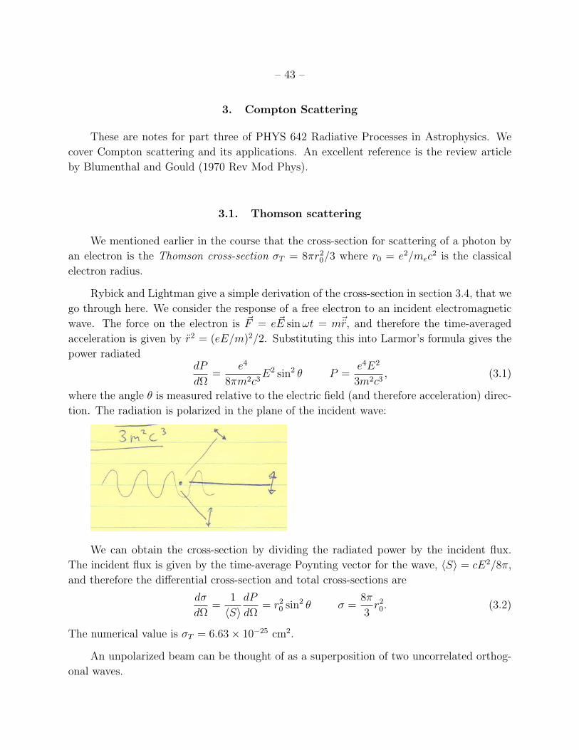
where the angle ✓ is measured relative to the electric field (and therefore acceleration) direc-

tion. The radiation is polarized in the plane of the incident wave:

We can obtain the cross-section by dividing the radiated power by the incident flux.

The incident flux is given by the time-average Poynting vector for the wave, hSi = cE2/8⇡,

and therefore the di↵erential cross-section and total cross-sections are

d�

d⌦=

1

hSi

dP

d⌦= r2

0

sin2 ✓ � =8⇡

3r2

0

. (3.2)

The numerical value is �T = 6.63⇥ 10�25 cm2.

An unpolarized beam can be thought of as a superposition of two uncorrelated orthog-

onal waves.

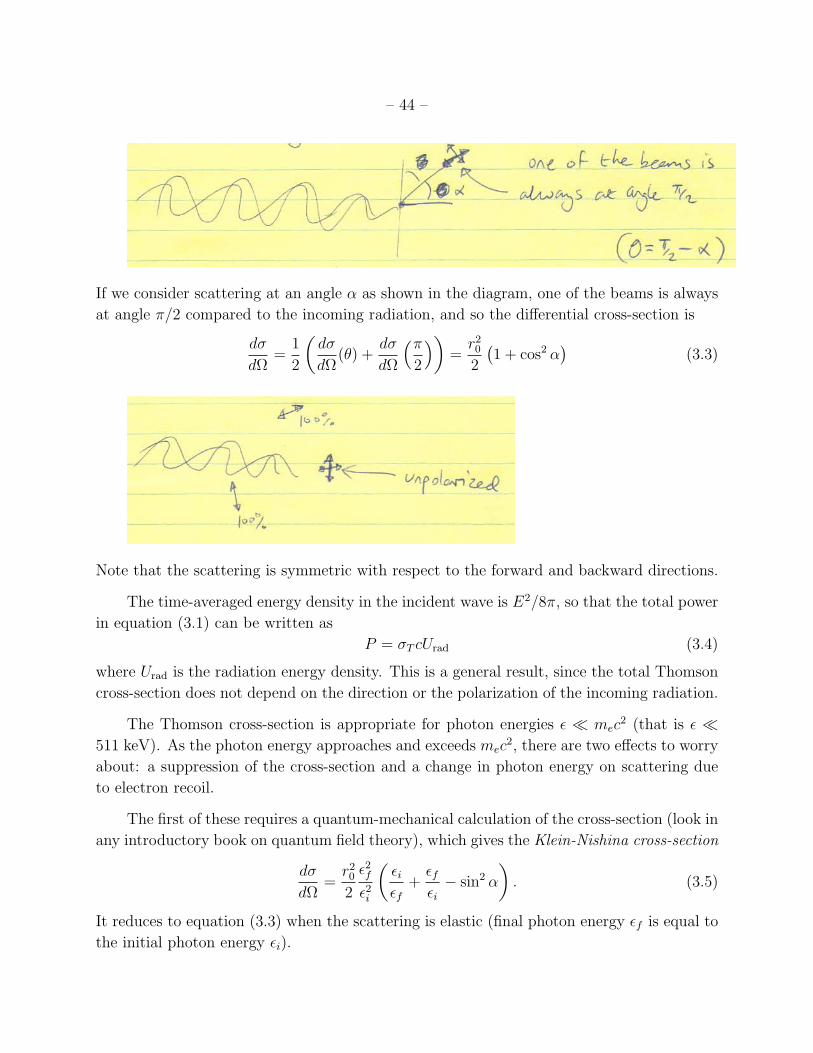
– 44 –

If we consider scattering at an angle ↵ as shown in the diagram, one of the beams is always

at angle ⇡/2 compared to the incoming radiation, and so the di↵erential cross-section is

d�

d⌦=

1

2

✓d�

d⌦(✓) +

d�

d⌦

⇣⇡2

⌘◆=

r2

0

2

�1 + cos2 ↵

�(3.3)

Note that the scattering is symmetric with respect to the forward and backward directions.

The time-averaged energy density in the incident wave is E2/8⇡, so that the total power

in equation (3.1) can be written as

P = �T cUrad

(3.4)

where Urad

is the radiation energy density. This is a general result, since the total Thomson

cross-section does not depend on the direction or the polarization of the incoming radiation.

The Thomson cross-section is appropriate for photon energies ✏ ⌧ mec2 (that is ✏ ⌧

511 keV). As the photon energy approaches and exceeds mec2, there are two e↵ects to worry

about: a suppression of the cross-section and a change in photon energy on scattering due

to electron recoil.

The first of these requires a quantum-mechanical calculation of the cross-section (look in

any introductory book on quantum field theory), which gives the Klein-Nishina cross-section

d�

d⌦=

r2

0

2

✏2f✏2i

✓✏i✏f

+✏f✏i� sin2 ↵

◆. (3.5)

It reduces to equation (3.3) when the scattering is elastic (final photon energy ✏f is equal to

the initial photon energy ✏i).

– 45 –

The final photon energy ✏f is given by a consideration of the kinematics of the scattering,

which we look at in the next section. The resulting total cross-section is given by Rybicki

and Lightman equation (7.5). The limits are

� ⇡ �T (1� 2x + ...) x⌧ 1 (3.6)

=3

8�T

1

x

✓ln 2x +

1

2

◆⇠ �T

✓mec

2

✏

◆x� 1 (3.7)

where x = ✏i/mec2. The cross-section is Thomson for low photon energies and suppressed

at high photon energies.

3.2. Kinematics of Compton scattering

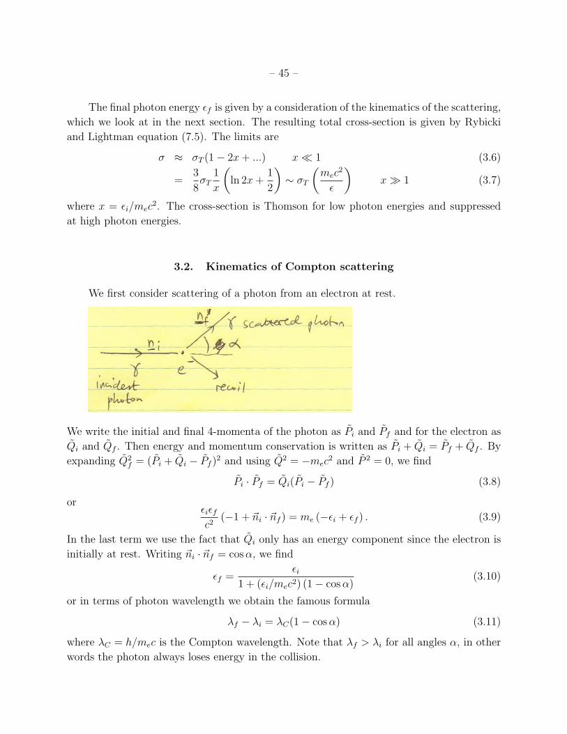
We first consider scattering of a photon from an electron at rest.

We write the initial and final 4-momenta of the photon as Pi and Pf and for the electron as

Qi and Qf . Then energy and momentum conservation is written as Pi + Qi = Pf + Qf . By

expanding Q2

f = (Pi + Qi � Pf )2 and using Q2 = �mec2 and P 2 = 0, we find

Pi · Pf = Qi(Pi � Pf ) (3.8)

or✏i✏fc2

(�1 + ~ni · ~nf ) = me (�✏i + ✏f ) . (3.9)

In the last term we use the fact that Qi only has an energy component since the electron is

initially at rest. Writing ~ni · ~nf = cos↵, we find

✏f =✏i

1 + (✏i/mec2) (1� cos↵)(3.10)

or in terms of photon wavelength we obtain the famous formula

�f � �i = �C(1� cos↵) (3.11)

where �C = h/mec is the Compton wavelength. Note that �f > �i for all angles ↵, in other

words the photon always loses energy in the collision.

– 46 –

3.3. Inverse Compton scattering

If the electron is moving with velocity v, energy can be transferred from the electron

to the photon, which is known as inverse Compton scattering. In the electron rest frame,

our previous result holds, but now written in terms of rest-frame variables which we indicate

with a prime:

✏0f =✏0i

1 + (✏0i/mec2) (1� cos↵0). (3.12)

The angle ↵0 = ✓0f � ✓0i is the scattering angle in the rest frame.

We just need to transform back into the lab frame. The angle ✓i is the initial angle

between the electron and photon propagation directions, so that

Pi =✏ic

(1, cos ✓i, sin ✓i, 0) . (3.13)

The Lorentz transform is

P 0i =

0

@� ��� 0

��� � 0

0 0 1

1

A Pi (3.14)

giving

P 0i =

✏ic

(�(1� � cos ✓i),��� + � cos ✓i, sin ✓i, 0) (3.15)

and

✏0i = ✏i�(1� � cos ✓i). (3.16)

The limits of this expression are (1) for ✓i ⇡ ⇡ (head on collision) ✏0i = ✏i�(1+�) or for large

�, ✏0i ⇡ 2�✏i, and (2) for ✓i ⇡ 0 (photon approaches from behind) we get ✏0i = ✏i�(1 � �) =

✏i/(�(1 + �)) or for large �, ✏0i ⇡ ✏i/2�. Similarly, the reverse transform gives

✏f = ✏0f�(1 + � cos ✓0f ). (3.17)

We see that the maximum energy we can expect is therefore ✏f,max

= 4�2✏i.

The general rule is that the photon energies before scattering, in the electron rest frame,

and after scattering are roughly in the ratios 1 : � : �2. A photon scattering from a relativistic

electron can therefore undergo a tremendous increase in frequency, scattering radio photons

into the optical to X-ray range for example, depending on the value of �.

As well as being boosted in energy, the photon distribution is strongly beamed in the rest

frame. Writing P 0i = (✏0i/c)(1, cos ✓0i, sin ✓

0i, 0), we see that cos ✓0i✏

0i/c = (✏i/c)(��� + � cos ✓i)

which gives the standard aberration formula (e.g. RL 4.86)

cos ✓0i =cos ✓i � �

1� � cos ✓i

. (3.18)

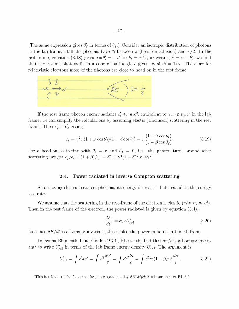
– 47 –

(The same expression gives ✓0f in terms of ✓f .) Consider an isotropic distribution of photons

in the lab frame. Half the photons have ✓i between ⇡ (head on collision) and ⇡/2. In the

rest frame, equation (3.18) gives cos ✓0i = �� for ✓i = ⇡/2, or writing � = ⇡ � ✓0i, we find

that these same photons lie in a cone of half angle � given by sin � = 1/�. Therefore for

relativistic electrons most of the photons are close to head on in the rest frame.

If the rest frame photon energy satisfies ✏0i ⌧ mec2, equivalent to �✏i ⌧ mec

2 in the lab

frame, we can simplify the calculations by assuming elastic (Thomson) scattering in the rest

frame. Then ✏0f = ✏0i, giving

✏f = �2✏i(1 + � cos ✓0f )(1� � cos ✓i) = ✏i(1� � cos ✓i)

(1� � cos ✓f ). (3.19)

For a head-on scattering with ✓i = ⇡ and ✓f = 0, i.e. the photon turns around after

scattering, we get ✏f/✏i = (1 + �)/(1� �) = �2(1 + �)2

⇡ 4�2.

3.4. Power radiated in inverse Compton scattering

As a moving electron scatters photons, its energy decreases. Let’s calculate the energy

loss rate.

We assume that the scattering in the rest-frame of the electron is elastic (�h⌫ ⌧ mec2).

Then in the rest frame of the electron, the power radiated is given by equation (3.4),

dE 0

dt0= �T cU 0

rad

(3.20)

but since dE/dt is a Lorentz invariant, this is also the power radiated in the lab frame.

Following Blumenthal and Gould (1970), RL use the fact that dn/✏ is a Lorentz invari-

ant7 to write U 0rad

in terms of the lab frame energy density Urad

. The argument is

U 0rad

=

Z✏0dn0 =

Z✏02

dn0

✏0=

Z✏02

dn

✏=

Z✏2�2(1� �µ)2

dn

✏. (3.21)

7This is related to the fact that the phase space density dN/d3~pd3~x is invariant; see RL 7.2.

– 48 –

Averaging over angles gives (assume isotropic radiation field)

1

2

Z1

�1

dµ(1� �µ)2 = 1 +�2

3(3.22)

and

U 0rad

= Urad

�2

✓1 +

�2

3

◆. (3.23)

There is another way to find U 0rad

, which is to transform the incident electric field

into the rest frame. For an EM wave/photon travelling at angle ✓ relative to the electron,

Ex = �E sin ✓, Ez = E cos ✓, and By = �E (since ~B = ~n ⇥ ~E). Now transform these

fields into the rest frame: E 0x = Ex = �E sin ✓, E 0

z = �(Ez + �B) = �E(cos ✓ � �). The

time-averaged energy density is

E 02

8⇡=

E2

8⇡

�1� µ2 + �2(µ� �)2

�=

E2

8⇡�2(1� µ�)2 (3.24)

which is the same as previously.

Equation (3.20) gives the power in scattered photons which are added to the radiation

field, but the scattering also removes energy from the radiation field at a rate �T cUrad

for an

isotropic photon distribution8. The di↵erence between these two rates must be supplied by

the energy of the electron. Therefore the rate of energy loss of the electrons is given by

�

dEe

dt= �T c (U 0

rad

� Urad

) (3.25)

or

�

dEe

dt= �T cU

rad

�2

✓1 +

�2

3

◆� 1

�=

4

3�2�2�T cU

rad

, (3.26)

where we use �2

� 1 = �2�2. This result is independent of the photon spectrum; applies for

an isotropic distribution and Thomson scattering in the rest frame. The average fractional

increase in photon energy is (4/3)�2�2.

When the energy transfer in the electron rest frame becomes significant, Blumenthal

and Gould (1970) showed that

�

dEe

dt=

4

3�2�2�T cU

rad

1�

63

10

�

mec2

h✏2i

h✏i

�, (3.27)

8You might wonder whether this formula would apply to an electron not at rest. Blumenthal and Gould1970 show that the rate of scatterings for photons moving at angle ✓ with respect to the electron is dn(✓)�

T

(c�v cos ✓). The cos term drops out when averaging over angles for an isotropic photon distribution.

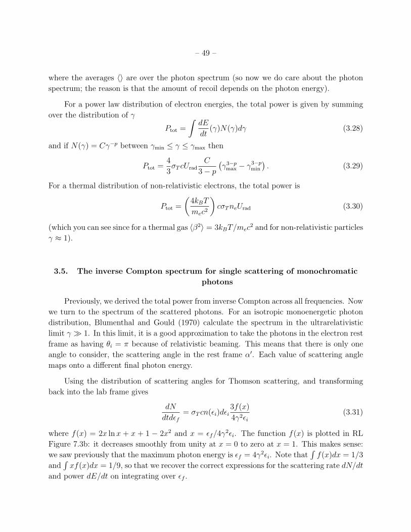
– 49 –

where the averages hi are over the photon spectrum (so now we do care about the photon

spectrum; the reason is that the amount of recoil depends on the photon energy).

For a power law distribution of electron energies, the total power is given by summing

over the distribution of �

Ptot

=

ZdE

dt(�)N(�)d� (3.28)

and if N(�) = C��p between �min

� �max

then

Ptot

=4

3�T cU

rad

C

3� p

��3�p

max

� �3�pmin

�. (3.29)

For a thermal distribution of non-relativistic electrons, the total power is

Ptot

=

✓4kBT

mec2

◆c�T neUrad

(3.30)

(which you can see since for a thermal gas h�2

i = 3kBT/mec2 and for non-relativistic particles

� ⇡ 1).

3.5. The inverse Compton spectrum for single scattering of monochromatic

photons

Previously, we derived the total power from inverse Compton across all frequencies. Now

we turn to the spectrum of the scattered photons. For an isotropic monoenergetic photon

distribution, Blumenthal and Gould (1970) calculate the spectrum in the ultrarelativistic

limit � � 1. In this limit, it is a good approximation to take the photons in the electron rest

frame as having ✓i = ⇡ because of relativistic beaming. This means that there is only one

angle to consider, the scattering angle in the rest frame ↵0. Each value of scattering angle

maps onto a di↵erent final photon energy.

Using the distribution of scattering angles for Thomson scattering, and transforming

back into the lab frame gives

dN

dtd✏f= �T cn(✏i)d✏i

3f(x)

4�2✏i(3.31)

where f(x) = 2x ln x + x + 1 � 2x2 and x = ✏f/4�2✏i. The function f(x) is plotted in RL

Figure 7.3b: it decreases smoothly from unity at x = 0 to zero at x = 1. This makes sense:

we saw previously that the maximum photon energy is ✏f = 4�2✏i. Note thatR

f(x)dx = 1/3

andR

xf(x)dx = 1/9, so that we recover the correct expressions for the scattering rate dN/dt

and power dE/dt on integrating over ✏f .

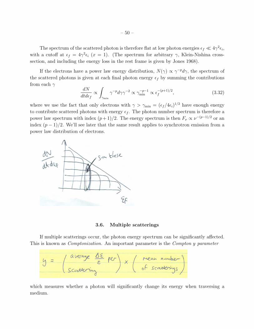
– 50 –

The spectrum of the scattered photon is therefore flat at low photon energies ✏f ⌧ 4�2✏i,

with a cuto↵ at ✏f = 4�2✏i (x = 1). (The spectrum for arbitrary �, Klein-Nishina cross-

section, and including the energy loss in the rest frame is given by Jones 1968).

If the electrons have a power law energy distribution, N(�) / ��pd�, the spectrum of

the scattered photons is given at each final photon energy ✏f by summing the contributions

from each �dN

dtd✏f/

Z

�min

��pd���2

/ ��p�1

min

/ ✏�(p+1)/2

f , (3.32)

where we use the fact that only electrons with � > �min

= (✏f/4✏i)1/2 have enough energy

to contribute scattered photons with energy ✏f . The photon number spectrum is therefore a

power law spectrum with index (p+1)/2. The energy spectrum is then F⌫ / ⌫�(p�1)/2 or an

index (p� 1)/2. We’ll see later that the same result applies to synchrotron emission from a

power law distribution of electrons.

3.6. Multiple scatterings

If multiple scatterings occur, the photon energy spectrum can be significantly a↵ected.

This is known as Comptonization. An important parameter is the Compton y parameter

which measures whether a photon will significantly change its energy when traversing a

medium.

– 51 –

Let’s look at each term separately. We saw previously that the average fractional change

in photon energy on scattering is (4/3)�2�2. For a thermal gas of non-relativistic electrons,

this is 4kBT/mec2 (since mehv

2

i/2 = 3kBT/2). However, this ignores electron recoil (we

assumed elastic scattering in the rest frame). We can estimate this from our earlier result

✏0f =✏0i

1 + (✏i/mec2)(1� cos↵0)⇡ ✏0i

✓1�

✏0imec2

(1� cos↵0)

◆. (3.33)

Averaging over angles gives �✏/✏ ⇡ �✏/mec2. Therefore,

�✏

✏=

✓4kBT

mec2

�

✏

mec2

◆. (3.34)

In the ultra-relativistic limit (� � 1), �✏/✏ ⇡ (4/3)�2 (the recoil term is negligible in this

limit).

The number of scatterings depends on the optical depth. We found in the section on

radiative transfer that the number of scatterings is max(⌧, ⌧ 2), where ⌧ ⇡ ⇢esR ⇡ ne�T R.

Therefore for a thermal gas of non-relativistic electrons

y =4kBT

mec2

max(⌧, ⌧ 2). (3.35)

How do multiple scatterings change the photon energy? If we start with a photon with

initial energy ✏0

⌧ kBT , then after N scatterings,

✏ = ✏0

✓1 +

4kBT

mec2

◆N

⇡ exp

✓4kBT

mec2

N

◆⇡ exp (y) . (3.36)

When the photon energy reaches ✏ = 4kBT , equation (3.34) shows that the photon energy

will no longer increase, that is we reach an equilibrium. By setting ⌧ 2 = N and ✏ = 4kBT in

equation (3.36), we find the optical depth required to reach equilibrium is

⌧ =

mec

2

4kBTln

✓4kBT

✏0

◆�1/2

. (3.37)

Because we are dealing with a fixed number of photons (scattering conserves photon

number), we expect the equilibrium distribution of photons to be a Bose-Einstein distribution

with a non-zero chemical potential µ, that is with energy density

U⌫d⌫ =8⇡h⌫3

c2

exp

✓h⌫

kBT+ µ

◆� 1

��1

d⌫. (3.38)

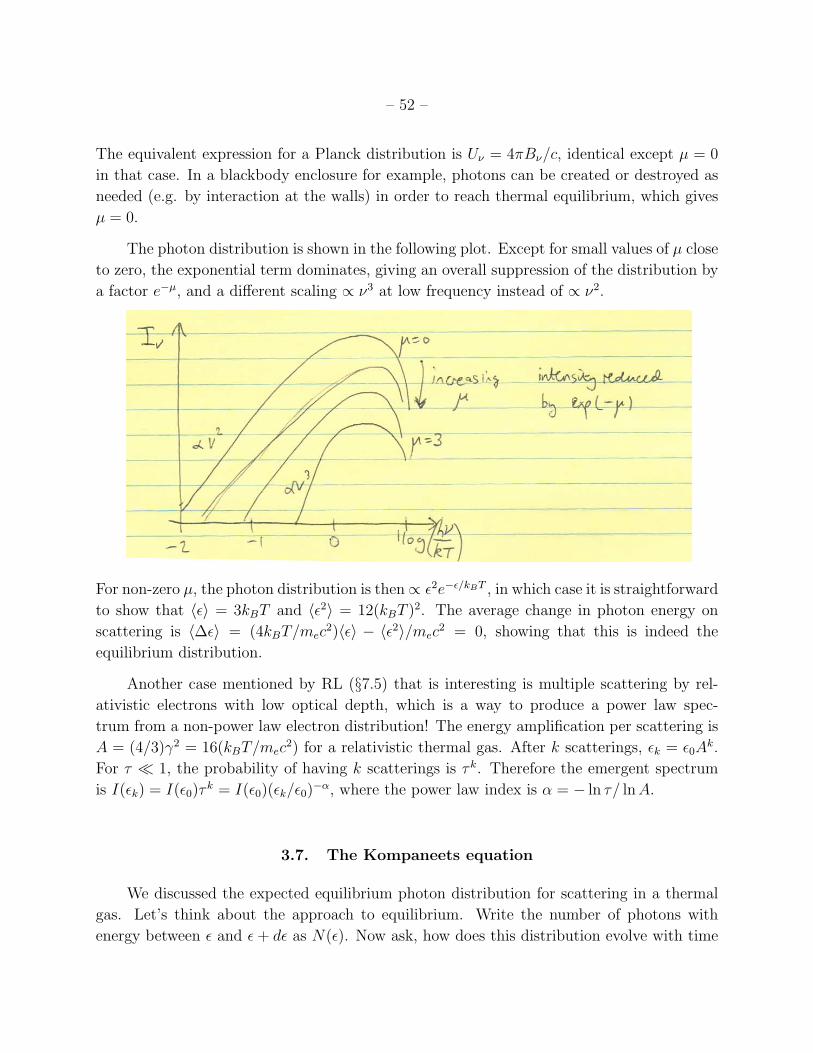
– 52 –

The equivalent expression for a Planck distribution is U⌫ = 4⇡B⌫/c, identical except µ = 0

in that case. In a blackbody enclosure for example, photons can be created or destroyed as

needed (e.g. by interaction at the walls) in order to reach thermal equilibrium, which gives

µ = 0.

The photon distribution is shown in the following plot. Except for small values of µ close

to zero, the exponential term dominates, giving an overall suppression of the distribution by

a factor e�µ, and a di↵erent scaling / ⌫3 at low frequency instead of / ⌫2.

For non-zero µ, the photon distribution is then/ ✏2e�✏/kBT , in which case it is straightforward

to show that h✏i = 3kBT and h✏2i = 12(kBT )2. The average change in photon energy on

scattering is h�✏i = (4kBT/mec2)h✏i � h✏2i/mec

2 = 0, showing that this is indeed the

equilibrium distribution.

Another case mentioned by RL (§7.5) that is interesting is multiple scattering by rel-

ativistic electrons with low optical depth, which is a way to produce a power law spec-

trum from a non-power law electron distribution! The energy amplification per scattering is

A = (4/3)�2 = 16(kBT/mec2) for a relativistic thermal gas. After k scatterings, ✏k = ✏

0

Ak.

For ⌧ ⌧ 1, the probability of having k scatterings is ⌧ k. Therefore the emergent spectrum

is I(✏k) = I(✏0

)⌧ k = I(✏0

)(✏k/✏0)�↵, where the power law index is ↵ = � ln ⌧/ ln A.

3.7. The Kompaneets equation

We discussed the expected equilibrium photon distribution for scattering in a thermal

gas. Let’s think about the approach to equilibrium. Write the number of photons with

energy between ✏ and ✏+ d✏ as N(✏). Now ask, how does this distribution evolve with time

– 53 –

as the scatterings occur? For each scattering, we can write down a probability distribution

for a change in the photon energy ✏! ✏+�, i.e. P (✏, �)d� is the probability that a photon

with energy ✏ changes its energy by an amount �. The normalization isR

d�P (✏, �) = 1

(the photon must change its energy by some amount).

Then the evolution of the photon distribution is given by

N(✏, t + �t)�N(✏, t) =

Zd� [N(✏��, t)P (✏��, �)�N(✏, t)P (✏, �)] (3.39)

where the timescale �t is a scattering timescale �t = ts = 1/ne�T c. For small �, we can

expand

N(✏��, t) ⇡ N(✏, t)��@N

@✏+

�2

2

@2N

@✏2+ ... (3.40)

P (✏��, �) ⇡ P (✏, �)��@P

@✏+

�2

2

@2P

@✏2+ ... (3.41)

which gives

N(✏, t + ts)�N(✏, t) = �@

@✏

Zd�NP� +

1

2

@2

@✏2

Zd�NP�2. (3.42)

Using this result and expanding N(t + ts) ⇡ N(t) + ts@N/@t, we obtain the Fokker-Planck

equation

ts@N

@t= �

@

@✏(h�iN) +

1

2

@2

@✏2�Nh�2

i

�. (3.43)

This is an advection-di↵usion equation in energy space.

For a thermal distribution of electrons,

h�i = ✏

✓4kBT

mec2

�

✏

mec2

◆h�2

i = ✏2✓

2kBT

mec2

◆. (3.44)

The second result is computed in RL §7.6 (compare RL eq. 7.54). Substituting these in and

simplifying gives

ts@N

@t= �

@

@✏

✓2✏N � ✏2

@N

@✏

◆✓kBT

mec2

◆�

✏2N

mec2

�(3.45)

Now to agree with RL, we switch notation to n(!) where !2n(!) / N(✏), and define

x = ~!/kBT . The result is

ts@n

@t=

✓kBT

mec2

◆1

x2

@

@x

x4

✓@n

@x+ n

◆�. (3.46)

– 54 –

The equilibrium solution (@n/@t = 0) is n / e�x or N / ✏2e�✏/kBT . This is the relativistic

Maxwell-Boltzmann distribution we discussed earlier.

Why didn’t we find the equilibrium distribution to be the Bose-Einstein distribution

n = (ex+↵� 1)�1? We should have included extra (1 + n) factors to account for the fact

that photons tend to mutual occupation of the same state (see RL eq. 7.48), i.e. the RHS

of equation (3.39) should be

Zd� [N(✏��, t)P (✏��, �)(1 + N(✏, t))�N(✏, t)P (✏, �)(1 + N(✏��, t))] . (3.47)

As we discussed earlier the extra terms are only important for µ approaching zero, which

indicates that multiple occupation of states is important. For non-zero µ the occupation

number is small and the extra 1 + n terms are no longer important. The particles then have

a Maxwell-Boltzmann distribution of energies.

With the extra terms, the analysis follows as before, but now the result is

ts@n

@t=

✓kBT

mec2

◆1

x2

@

@x

x4

✓@n

@x+ n + n2

◆�. (3.48)

This is the Kompaneets equation, which has the equilibrium solution n = (ex+↵� 1)�1.

3.8. Example: Sunyaev-Zeldovich e↵ect

The Sunyaev-Zeldovich or SZ e↵ect is a small distortion of the spectrum of the cosmic

microwave background (CMB) radiation due to inverse Compton scattering of CMB photons

by hot electrons in Galaxy clusters (for a review see Carlstrom, Holder, and Reese 2002

ARAA).

We can calculate the e↵ect by using the Kompaneets equation. Because Tgas

� Trad

,

the @n/@x term dominates on the RHS. To see this, note that x = h⌫/kBT ⌧ 1, and then

you can show that @n/@x ⇠ n/x for a Planck spectrum n = (ex� 1)�1. The Kompaneets

equation we need to solve is therefore

1

c

@n

@t=

✓ne�T

kBT

mec2

◆1

x2

@

@x

✓x4

@n

@x

◆. (3.49)

Following the path of a photon, dl = c dt, and so in terms of the Compton y parameter,

@n

@y=

1

x2

@

@x

✓x4

@n

@x

◆. (3.50)

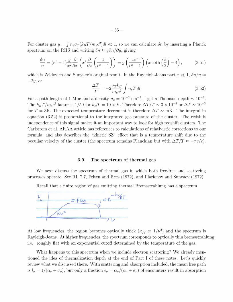
– 55 –

For cluster gas y =R

ne�T (kBT/mec2)dl ⌧ 1, so we can calculate �n by inserting a Planck

spectrum on the RHS and writing �n ⇡ y@n/@y, giving

�n

n= (ex

� 1)y

x2

@

@x

✓x4

@

@x

✓1

ex� 1

◆◆= y

✓xex

ex� 1

◆⇣x coth

⇣x

2

⌘� 4⌘

, (3.51)

which is Zeldovich and Sunyaev’s original result. In the Rayleigh-Jeans part x⌧ 1, �n/n ⇡

�2y, or�T

T= �2

�T kB

mec2

ZneT dl. (3.52)

For a path length of 1 Mpc and a density ne = 10�2 cm�3, I get a Thomson depth ⇠ 10�2.

The kBT/mec2 factor is 1/50 for kBT = 10 keV. Therefore �T/T ⇠ 3⇥ 10�4 or �T ⇠ 10�3

for T = 3K. The expected temperature decrement is therefore �T ⇠ mK. The integral in

equation (3.52) is proportional to the integrated gas pressure of the cluster. The redshift

independence of this signal makes it an important way to look for high redshift clusters. The

Carlstrom et al. ARAA article has references to calculations of relativistic corrections to our

formula, and also describes the “kinetic SZ” e↵ect that is a temperature shift due to the

peculiar velocity of the cluster (the spectrum remains Planckian but with �T/T ⇡ �⌧v/c).

3.9. The spectrum of thermal gas

We next discuss the spectrum of thermal gas in which both free-free and scattering

processes operate. See RL 7.7, Felten and Rees (1972), and Illarionov and Sunyaev (1972).

Recall that a finite region of gas emitting thermal Bremsstrahlung has a spectrum

At low frequencies, the region becomes optically thick (ff / 1/⌫2) and the spectrum is

Rayleigh-Jeans. At higher frequencies, the spectrum corresponds to optically thin bremsstrahlung,

i.e. roughly flat with an exponential cuto↵ determined by the temperature of the gas.

What happens to this spectrum when we include electron scattering? We already men-

tioned the idea of thermalization depth at the end of Part I of these notes. Let’s quickly

review what we discussed there. With scattering and absorption included, the mean free path

is l⌫ = 1/(↵⌫ + �⌫), but only a fraction ✏⌫ = ↵⌫/(↵⌫ + �⌫) of encounters result in absorption

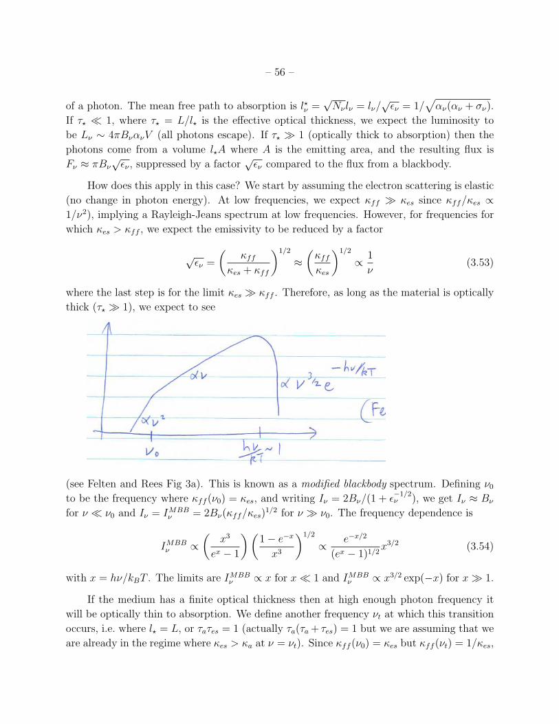
– 56 –

of a photon. The mean free path to absorption is l?⌫ =p

N⌫l⌫ = l⌫/p

✏⌫ = 1/p↵⌫(↵⌫ + �⌫).

If ⌧? ⌧ 1, where ⌧? = L/l? is the e↵ective optical thickness, we expect the luminosity to

be L⌫ ⇠ 4⇡B⌫↵⌫V (all photons escape). If ⌧? � 1 (optically thick to absorption) then the

photons come from a volume l?A where A is the emitting area, and the resulting flux is

F⌫ ⇡ ⇡B⌫p

✏⌫ , suppressed by a factorp

✏⌫ compared to the flux from a blackbody.

How does this apply in this case? We start by assuming the electron scattering is elastic

(no change in photon energy). At low frequencies, we expect ff � es since ff/es /

1/⌫2), implying a Rayleigh-Jeans spectrum at low frequencies. However, for frequencies for

which es > ff , we expect the emissivity to be reduced by a factor

p

✏⌫ =

✓ff

es + ff

◆1/2

⇡

✓ff

es

◆1/2

/

1

⌫(3.53)

where the last step is for the limit es � ff . Therefore, as long as the material is optically

thick (⌧? � 1), we expect to see

(see Felten and Rees Fig 3a). This is known as a modified blackbody spectrum. Defining ⌫0

to be the frequency where ff (⌫0

) = es, and writing I⌫ = 2B⌫/(1 + ✏�1/2

⌫ ), we get I⌫ ⇡ B⌫

for ⌫ ⌧ ⌫0

and I⌫ = IMBB⌫ = 2B⌫(ff/es)1/2 for ⌫ � ⌫

0

. The frequency dependence is

IMBB⌫ /

✓x3

ex� 1

◆✓1� e�x

x3

◆1/2

/

e�x/2

(ex� 1)1/2

x3/2 (3.54)

with x = h⌫/kBT . The limits are IMBB⌫ / x for x⌧ 1 and IMBB

⌫ / x3/2 exp(�x) for x� 1.

If the medium has a finite optical thickness then at high enough photon frequency it

will be optically thin to absorption. We define another frequency ⌫t at which this transition

occurs, i.e. where l? = L, or ⌧a⌧es = 1 (actually ⌧a(⌧a + ⌧es) = 1 but we are assuming that we

are already in the regime where es > a at ⌫ = ⌫t). Since ff (⌫0

) = es but ff (⌫t) = 1/es,

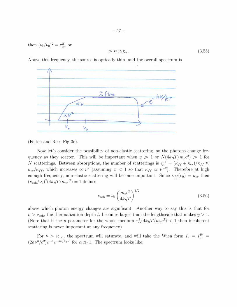
– 57 –

then (⌫t/⌫0

)2 = ⌧ 2

es, or

⌫t ⇡ ⌫0

⌧es. (3.55)

Above this frequency, the source is optically thin, and the overall spectrum is

(Felten and Rees Fig 3c).

Now let’s consider the possibility of non-elastic scattering, so the photons change fre-

quency as they scatter. This will be important when y � 1 or N(4kBT/mec2) � 1 for

N scatterings. Between absorptions, the number of scatterings is ✏�1

⌫ = (ff + es)/ff ⇡

es/ff , which increases / ⌫2 (assuming x < 1 so that ff / ⌫�2). Therefore at high

enough frequency, non-elastic scattering will become important. Since ff (⌫0

) = es then

(⌫coh

/⌫0

)2(4kBT/mec2) = 1 defines

⌫coh

= ⌫0

✓mec

2

4kBT

◆1/2

(3.56)

above which photon energy changes are significant. Another way to say this is that for

⌫ > ⌫coh

, the thermalization depth l? becomes larger than the lengthscale that makes y > 1.

(Note that if the y parameter for the whole medium ⌧ 2

es(4kBT/mec2) < 1 then incoherent

scattering is never important at any frequency).

For ⌫ > ⌫coh

, the spectrum will saturate, and will take the Wien form I⌫ = IW⌫ =

(2h⌫3/c2)e�↵e�h⌫/kBT for ↵� 1. The spectrum looks like:

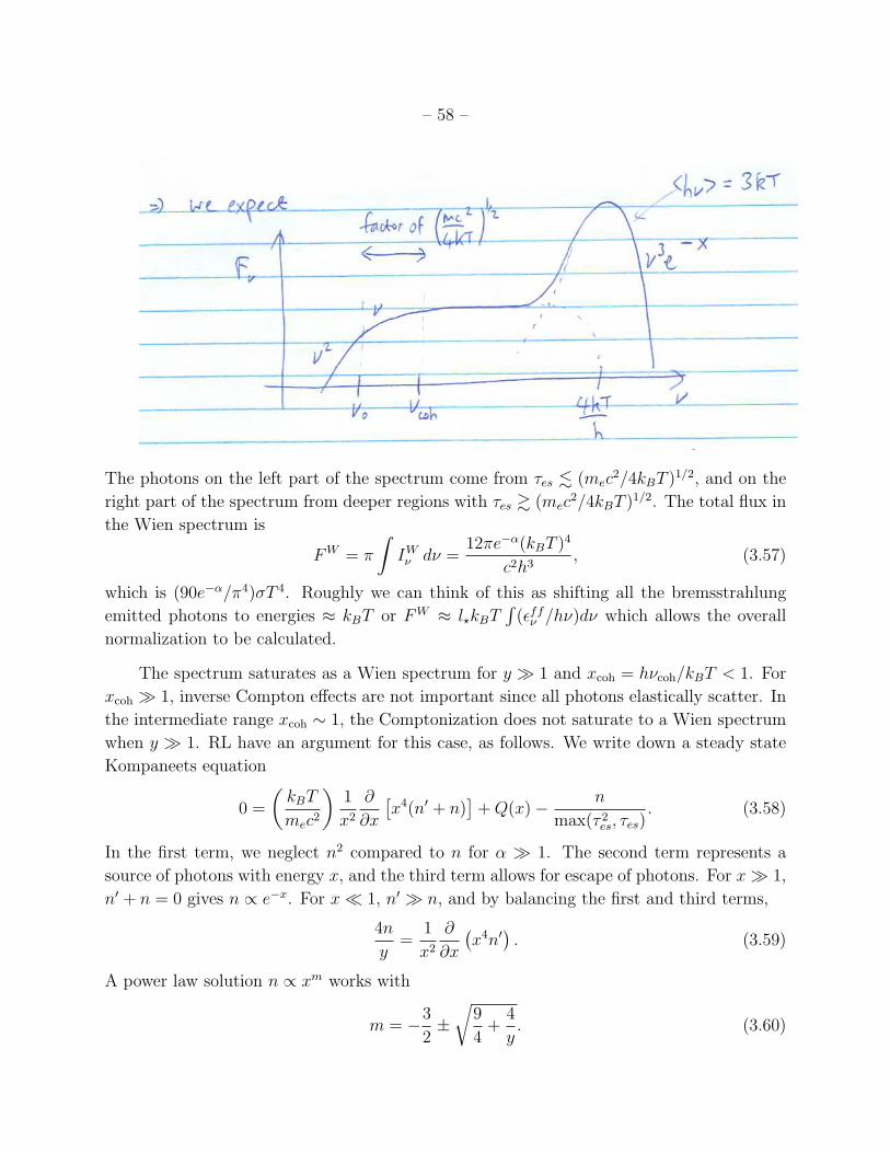
– 58 –

The photons on the left part of the spectrum come from ⌧es . (mec2/4kBT )1/2, and on the

right part of the spectrum from deeper regions with ⌧es & (mec2/4kBT )1/2. The total flux in

the Wien spectrum is

FW = ⇡

ZIW⌫ d⌫ =

12⇡e�↵(kBT )4

c2h3

, (3.57)

which is (90e�↵/⇡4)�T 4. Roughly we can think of this as shifting all the bremsstrahlung

emitted photons to energies ⇡ kBT or FW⇡ l?kBT

R(✏ff

⌫ /h⌫)d⌫ which allows the overall

normalization to be calculated.

The spectrum saturates as a Wien spectrum for y � 1 and xcoh

= h⌫coh

/kBT < 1. For

xcoh

� 1, inverse Compton e↵ects are not important since all photons elastically scatter. In

the intermediate range xcoh

⇠ 1, the Comptonization does not saturate to a Wien spectrum

when y � 1. RL have an argument for this case, as follows. We write down a steady state

Kompaneets equation

0 =

✓kBT

mec2

◆1

x2

@

@x

⇥x4(n0 + n)

⇤+ Q(x)�

n

max(⌧ 2

es, ⌧es). (3.58)

In the first term, we neglect n2 compared to n for ↵ � 1. The second term represents a

source of photons with energy x, and the third term allows for escape of photons. For x� 1,

n0 + n = 0 gives n / e�x. For x⌧ 1, n0 � n, and by balancing the first and third terms,

4n

y=

1

x2

@

@x

�x4n0

�. (3.59)

A power law solution n / xm works with

m = �3

2±

r9

4+

4

y. (3.60)

– 59 –

For y � 1 m = 0,�3 which gives either I⌫ / x3 or constant. For y ⌧ 1, I⌫ / ⌫3+m.

See Pozdniakov, Sobol, and Sunyaev (1983) for Monte Carlo calculations of spectra in this

regime. I’ve included a Figure from their paper below. It shows the change in the spectrum

with increasing y. I’ve also included a cartoon from that paper that shows astrophysical

environments where Comptonization is likely to be important.

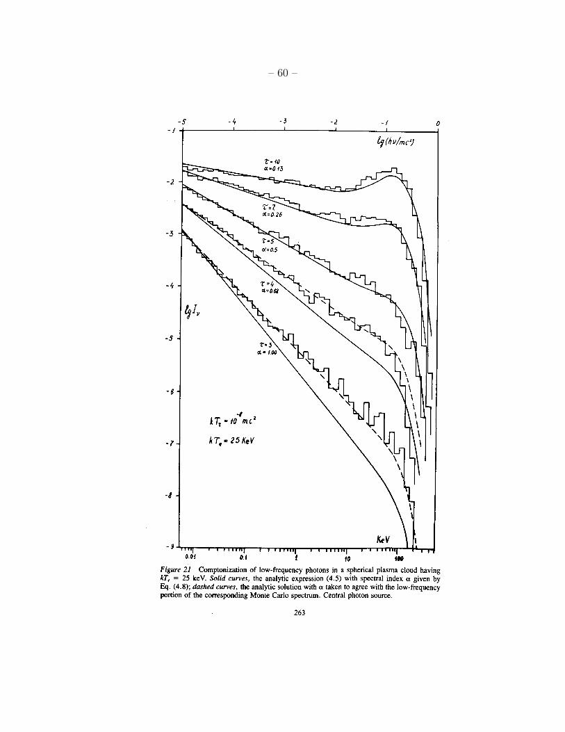
– 60 –

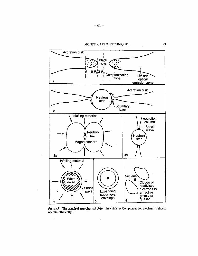
– 61 –

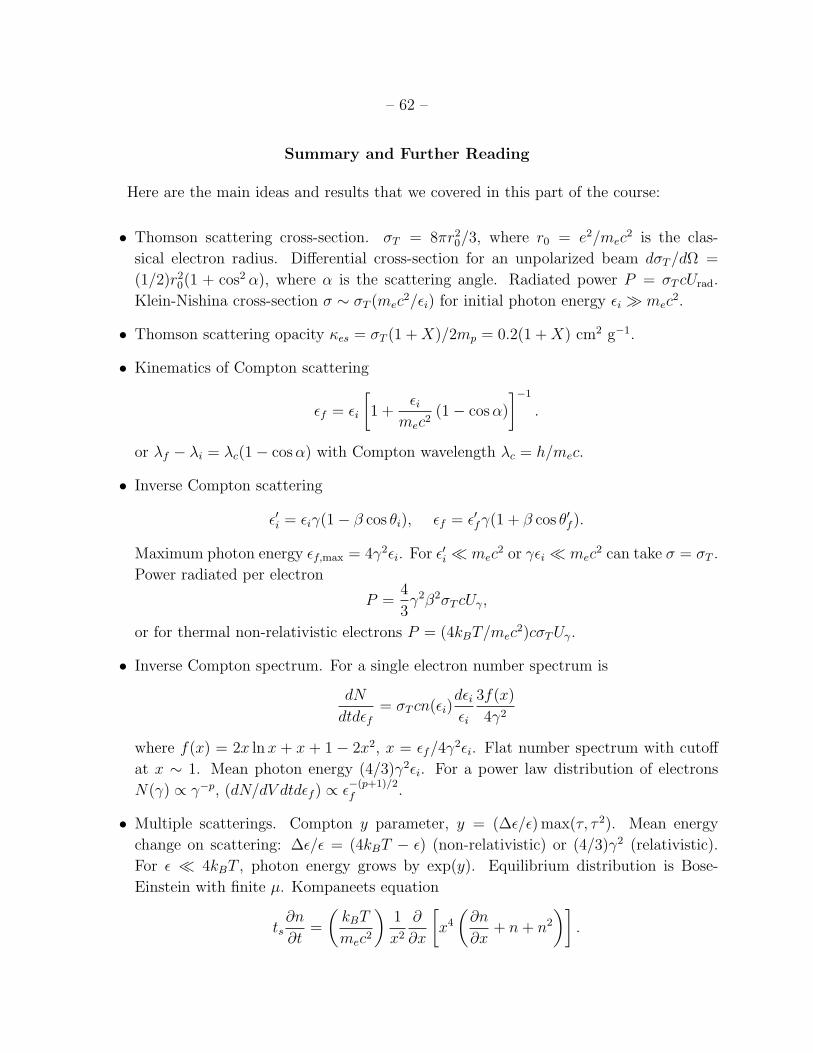
– 62 –

Summary and Further Reading

Here are the main ideas and results that we covered in this part of the course:

• Thomson scattering cross-section. �T = 8⇡r2

0

/3, where r0

= e2/mec2 is the clas-

sical electron radius. Di↵erential cross-section for an unpolarized beam d�T /d⌦ =

(1/2)r2

0

(1 + cos2 ↵), where ↵ is the scattering angle. Radiated power P = �T cUrad

.

Klein-Nishina cross-section � ⇠ �T (mec2/✏i) for initial photon energy ✏i � mec

2.

• Thomson scattering opacity es = �T (1 + X)/2mp = 0.2(1 + X) cm2 g�1.

• Kinematics of Compton scattering

✏f = ✏i

1 +

✏imec2

(1� cos↵)

��1

.

or �f � �i = �c(1� cos↵) with Compton wavelength �c = h/mec.

• Inverse Compton scattering

✏0i = ✏i�(1� � cos ✓i), ✏f = ✏0f�(1 + � cos ✓0f ).

Maximum photon energy ✏f,max

= 4�2✏i. For ✏0i ⌧ mec2 or �✏i ⌧ mec

2 can take � = �T .

Power radiated per electron

P =4

3�2�2�T cU�,

or for thermal non-relativistic electrons P = (4kBT/mec2)c�T U�.

• Inverse Compton spectrum. For a single electron number spectrum is

dN

dtd✏f= �T cn(✏i)

d✏i✏i

3f(x)

4�2

where f(x) = 2x ln x + x + 1 � 2x2, x = ✏f/4�2✏i. Flat number spectrum with cuto↵

at x ⇠ 1. Mean photon energy (4/3)�2✏i. For a power law distribution of electrons

N(�) / ��p, (dN/dV dtd✏f ) / ✏�(p+1)/2

f .

• Multiple scatterings. Compton y parameter, y = (�✏/✏) max(⌧, ⌧ 2). Mean energy

change on scattering: �✏/✏ = (4kBT � ✏) (non-relativistic) or (4/3)�2 (relativistic).

For ✏ ⌧ 4kBT , photon energy grows by exp(y). Equilibrium distribution is Bose-

Einstein with finite µ. Kompaneets equation

ts@n

@t=

✓kBT

mec2

◆1

x2

@

@x

x4

✓@n

@x+ n + n2

◆�.

– 63 –

• Applications. Sunyaev-Zeldovich e↵ect: �T/T = �2R

ne�T (kBT/mec2)dl. Spectrum

of thermal gas including free-free and scattering processes. Modified blackbody spec-

trum.

Reading

• RL chapter 7. Longair.

• Kinematic of Compton: see Blumenthal & Gould 1970, Rev Mod Phys, 42, 237

• Inverse Compton spectrum: Jones (1968) Phys Rev 167, 1159

• Sunyaev (1980) Sv A Lett, 6, 213 one of the original papers on SZ e↵ect. See also the

ARAA article by Carlstrom, Holder, & Reese (2002).

• Felten & Rees (1972), Illarionov & Sunyaev (1972) spectrum of thermal gas includ-

ing free-free and electron scattering. Unsaturated Compton spectra are calculated by

Pozdniakov, Sobol, & Sunyaev (1983).

– 64 –

4. Synchrotron Radiation

These are notes for part four of PHYS 642 Radiative Processes in Astrophysics. Syn-

chrotron radiation is radiation from particles accelerated by magnetic fields. For non-

relativistic electrons, the radiation is at the gyration frequency ! = eB/mec and is known

as cyclotron radiation. However, for relativistic particles, the emission extends to higher

frequencies, and we then describe the radiation as synchrotron radiation. We also include

a discussion of Fermi acceleration of high energy particles, and the evolution of the energy

spectrum.

4.1. Power radiated by a relativistic particle

First, we want to extend Larmor’s formula to relativistic electrons. To do this, recall

the “four-acceleration” a = du/d⌧ where u = (c, ~u) is the four-velocity, and d⌧ is the interval

of proper time, d⌧ = ds/c, ds2 = c2dt2 � |d~x|2 = c2dt2/�2.

Let’s evaluate a in the rest frame of the particle, where d⌧ = dt0. First note that

d�0/dt0 = 0 since

d�0

dt0=

d

dt0

✓1�

~u0 · ~u0

c2

◆�1/2

=�3

2c2

d

dt0(~u0 · ~u0) =

�3

c2

~u0 ·d~u0

dt0= 0 (4.1)

since ~u0 = 0 in the rest frame. Therefore a0 = du0/dt0 = (0,~a0), and so Larmor’s formula

gives the power radiated in the rest frame

P =2q2

3c3

|~a0|2 =

2q2

3c3

a0 · a0. (4.2)

The norm of a four vector is Lorentz invariant (the same in all reference frames), meaning

that we can write the general form of Larmor’s formula as

P =2q2

3c3

a · a (4.3)

where a is the four-acceleration in the frame of interest.

In the lab frame,

a · a = �

✓c�

d�

dt

◆2

+

✓�

d

dt(�~u)

◆2

. (4.4)

Using d�/dt = �3~u · ~a/c2, this is

a · a = �4

|~a|2 +�6 (~u · ~a)2

c2

. (4.5)

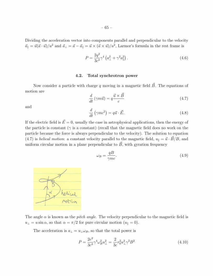
– 65 –

Dividing the acceleration vector into components parallel and perpendicular to the velocity

~ak = ~u(~a · ~u)/u2 and ~a? = ~a� ~ak = ~u⇥ (~a⇥ ~u)/u2, Larmor’s formula in the rest frame is

P =2q2

3c3

�4

�a2

? + �2a2

k�. (4.6)

4.2. Total synchrotron power

Now consider a particle with charge q moving in a magnetic field ~B. The equations of

motion ared

dt(�m~u) = q

~u⇥ ~B

c(4.7)

andd

dt

��mc2

�= q~u ·

~E. (4.8)

If the electric field is ~E = 0, usually the case in astrophysical applications, then the energy of

the particle is constant (� is a constant) (recall that the magnetic field does no work on the

particle because the force is always perpendicular to the velocity). The solution to equation

(4.7) is helical motion: a constant velocity parallel to the magnetic field, uk = ~u ·

~B/B, and

uniform circular motion in a plane perpendicular to ~B, with gyration frequency

!B =qB

�mc. (4.9)

The angle ↵ is known as the pitch angle. The velocity perpendicular to the magnetic field is

u? = u sin↵, so that ↵ = ⇡/2 for pure circular motion (uk = 0).

The acceleration is a? = u?!B, so that the total power is

P =2e2

3c3

�4!2

Bu2

? =2

3cr2

0

u2

?�2B2 (4.10)

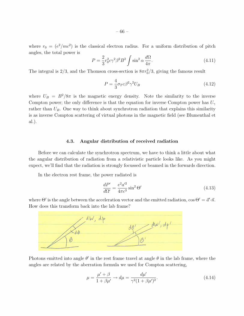
– 66 –

where r0

= (e2/mc2) is the classical electron radius. For a uniform distribution of pitch

angles, the total power is

P =2

3r2

0

c�2�2B2

Zsin2 ↵

d⌦

4⇡. (4.11)

The integral is 2/3, and the Thomson cross-section is 8⇡r2

0

/3, giving the famous result

P =4

3�T c�2�2UB (4.12)

where UB = B2/8⇡ is the magnetic energy density. Note the similarity to the inverse

Compton power; the only di↵erence is that the equation for inverse Compton power has U�

rather than UB. One way to think about synchrotron radiation that explains this similarity

is as inverse Compton scattering of virtual photons in the magnetic field (see Blumenthal et

al.).

4.3. Angular distribution of received radiation

Before we can calculate the synchrotron spectrum, we have to think a little about what

the angular distribution of radiation from a relativistic particle looks like. As you might

expect, we’ll find that the radiation is strongly focussed or beamed in the forwards direction.

In the electron rest frame, the power radiated is

dP 0

d⌦0=

e2a02

4⇡c3

sin2 ⇥0 (4.13)

where ⇥0 is the angle between the acceleration vector and the emitted radiation, cos ⇥0 = ~a0·~n.

How does this transform back into the lab frame?

Photons emitted into angle ✓0 in the rest frame travel at angle ✓ in the lab frame, where the

angles are related by the aberration formula we used for Compton scattering,

µ =µ0 + �

1 + �µ0! dµ =

dµ0

�2(1 + �µ0)2

. (4.14)

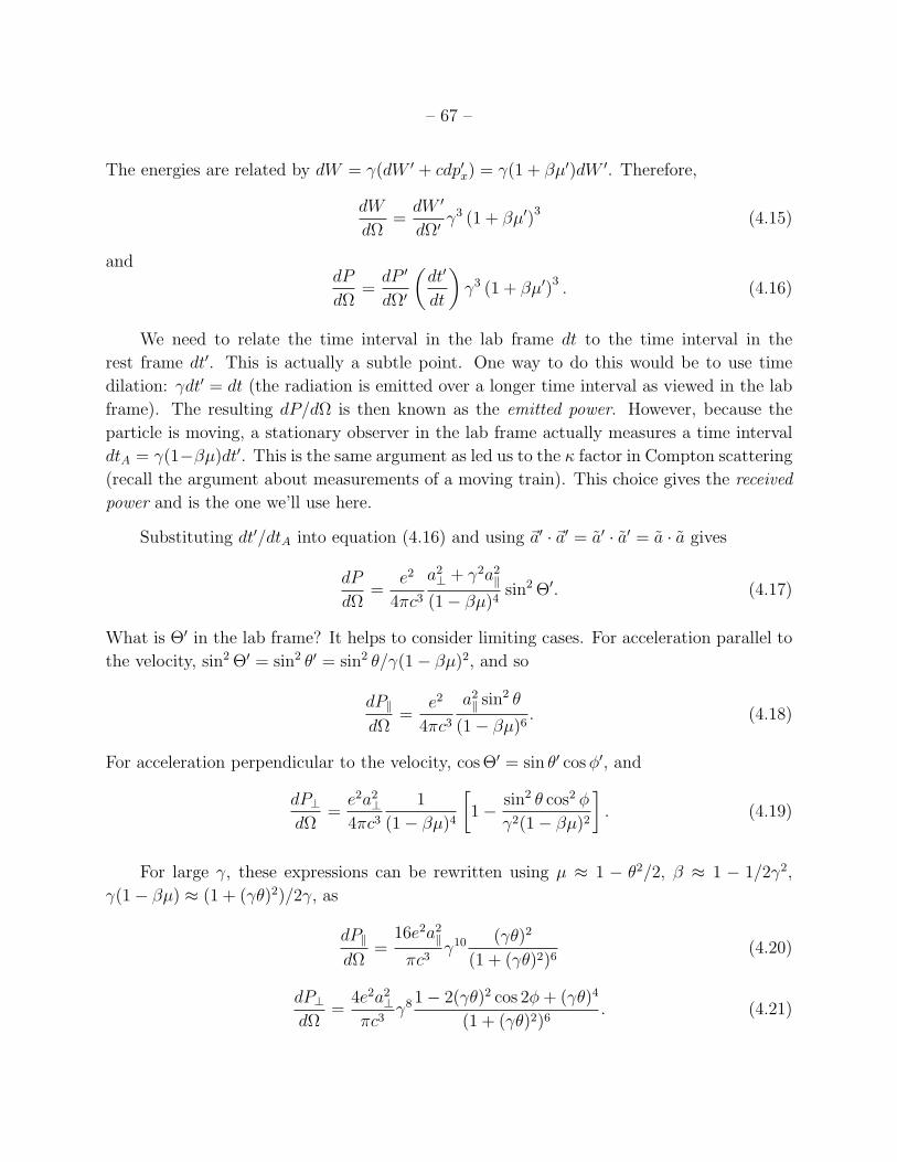
– 67 –

The energies are related by dW = �(dW 0 + cdp0x) = �(1 + �µ0)dW 0. Therefore,

dW

d⌦=

dW 0

d⌦0�3 (1 + �µ0)3 (4.15)

anddP

d⌦=

dP 0

d⌦0

✓dt0

dt

◆�3 (1 + �µ0)3

. (4.16)

We need to relate the time interval in the lab frame dt to the time interval in the

rest frame dt0. This is actually a subtle point. One way to do this would be to use time

dilation: �dt0 = dt (the radiation is emitted over a longer time interval as viewed in the lab

frame). The resulting dP/d⌦ is then known as the emitted power. However, because the

particle is moving, a stationary observer in the lab frame actually measures a time interval

dtA = �(1��µ)dt0. This is the same argument as led us to the factor in Compton scattering

(recall the argument about measurements of a moving train). This choice gives the received

power and is the one we’ll use here.

Substituting dt0/dtA into equation (4.16) and using ~a0 · ~a0 = a0 · a0 = a · a gives

dP

d⌦=

e2

4⇡c3

a2

? + �2a2

k

(1� �µ)4

sin2 ⇥0. (4.17)

What is ⇥0 in the lab frame? It helps to consider limiting cases. For acceleration parallel to

the velocity, sin2 ⇥0 = sin2 ✓0 = sin2 ✓/�(1� �µ)2, and so

dPkd⌦

=e2

4⇡c3

a2

k sin2 ✓

(1� �µ)6

. (4.18)

For acceleration perpendicular to the velocity, cos ⇥0 = sin ✓0 cos�0, and

dP?d⌦

=e2a2

?4⇡c3

1

(1� �µ)4

1�

sin2 ✓ cos2 �

�2(1� �µ)2

�. (4.19)

For large �, these expressions can be rewritten using µ ⇡ 1 � ✓2/2, � ⇡ 1 � 1/2�2,

�(1� �µ) ⇡ (1 + (�✓)2)/2�, as

dPkd⌦

=16e2a2

k

⇡c3

�10

(�✓)2

(1 + (�✓)2)6

(4.20)

dP?d⌦

=4e2a2

?⇡c3

�8

1� 2(�✓)2 cos 2�+ (�✓)4

(1 + (�✓)2)6

. (4.21)

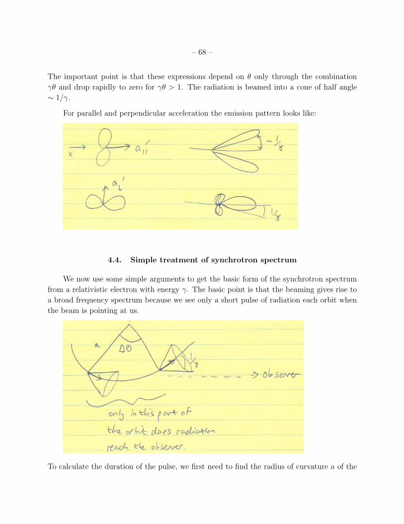
– 68 –

The important point is that these expressions depend on ✓ only through the combination

�✓ and drop rapidly to zero for �✓ > 1. The radiation is beamed into a cone of half angle

⇠ 1/�.

For parallel and perpendicular acceleration the emission pattern looks like:

4.4. Simple treatment of synchrotron spectrum

We now use some simple arguments to get the basic form of the synchrotron spectrum

from a relativistic electron with energy �. The basic point is that the beaming gives rise to

a broad frequency spectrum because we see only a short pulse of radiation each orbit when

the beam is pointing at us.

To calculate the duration of the pulse, we first need to find the radius of curvature a of the

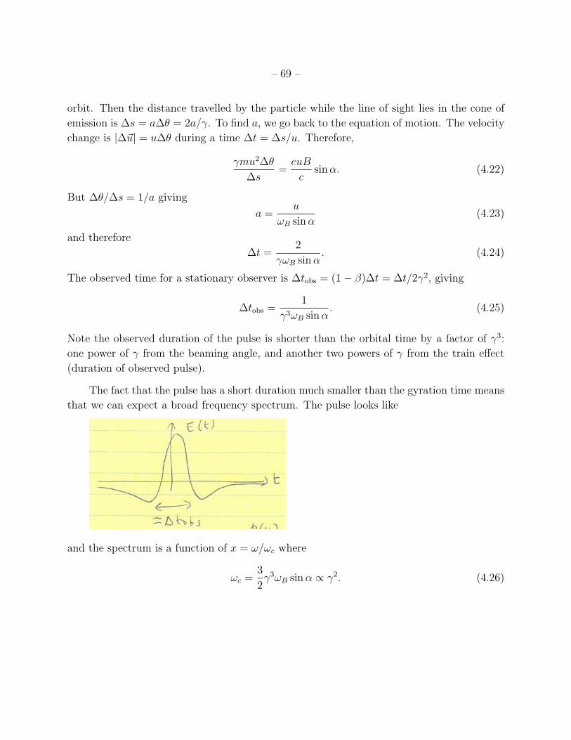
– 69 –

orbit. Then the distance travelled by the particle while the line of sight lies in the cone of

emission is �s = a�✓ = 2a/�. To find a, we go back to the equation of motion. The velocity

change is |�~u| = u�✓ during a time �t = �s/u. Therefore,

�mu2�✓

�s=

euB

csin↵. (4.22)

But �✓/�s = 1/a giving

a =u

!B sin↵(4.23)

and therefore

�t =2

�!B sin↵. (4.24)

The observed time for a stationary observer is �tobs

= (1� �)�t = �t/2�2, giving

�tobs

=1

�3!B sin↵. (4.25)

Note the observed duration of the pulse is shorter than the orbital time by a factor of �3:

one power of � from the beaming angle, and another two powers of � from the train e↵ect

(duration of observed pulse).

The fact that the pulse has a short duration much smaller than the gyration time means

that we can expect a broad frequency spectrum. The pulse looks like

and the spectrum is a function of x = !/!c where

!c =3

2�3!B sin↵ / �2. (4.26)

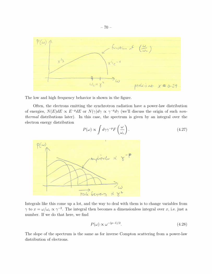
– 70 –

The low and high frequency behavior is shown in the figure.

Often, the electrons emitting the synchrotron radiation have a power-law distribution

of energies, N(E)dE / E�pdE or N(�)d� / ��pd� (we’ll discuss the origin of such non-

thermal distributions later). In this case, the spectrum is given by an integral over the

electron energy distribution

P (!) /

Zd���pF

✓!

!c

◆. (4.27)

Integrals like this come up a lot, and the way to deal with them is to change variables from

� to x = !/!c / ��2. The integral then becomes a dimensionless integral over x, i.e. just a

number. If we do that here, we find

P (!) / !�(p�1)/2. (4.28)

The slope of the spectrum is the same as for inverse Compton scattering from a power-law

distribution of electrons.

– 71 –

4.5. Detailed treatment of synchrotron spectrum

If you’ve looked in the books at the derivation of the synchrotron spectrum, you may

be a little nervous. Shu warns “The formal manipulations required for synchrotron theory

can get formidable” and Longair states ”I am not aware of any particularly simple way

of deriving [the synchrotron spectrum]..”. In fact it’s not that bad: in this section, we

outline the detailed derivation of the synchrotron spectrum, focussing on the methodology

and skipping a lot of the algebra. Here I follow the derivation given in Rybicki and Lightman

6.4, which in turn follows Jackson 14.6. Longair (volume 2) goes through it filling in more

of the steps. The classic paper is Westfold (1959) ApJ.

We start with the expressions for the radiation fields we derived earlier,

~Erad

=q

c

"~n⇥ (~n� ~�)⇥ ~�

3R

#~B

rad

= ~n⇥ ~Erad

(4.29)

where the notation [...] means evaluate at the retarded time t = t0+R/c and = 1�~n ·~u/c.

ThendW

d⌦=hR2~n ·

~Si

=c

4⇡

hR ~Ei

2

, (4.30)

and the Fourier component at frequency ! is

dW

d!d⌦=

q2

4⇡2c

����Z h

(~n⇥ (~n� ~�)⇥ ~�)�3

iei!tdt

����2

. (4.31)

Previously, we worked in the limit � ⌧ 1, but now we need to keep the relativistic factors.

A standard trick is to integrate by parts. First, change variables in the integral to

t0 = t�R(t0)/c. Since the source is very far from the observer, we can write R ⇡ R0

�~n ·~r(t0).

Then dt = dt0(1� ~n ·

~�) = dt0, and the integral is

dW

d!d⌦=

q2

4⇡2c

�����

Z(~n⇥ (~n� ~�)⇥ ~�)

2

ei!(t0�~r·~n/c)dt0

�����

2

. (4.32)

Now we can integrate by parts using

d

dt0

~n⇥ (~n⇥ ~�)

1� ~� · ~n

!=~n⇥ ((~n� ~�)⇥ ~�)

(1� ~� · ~n)2

(4.33)

to getdW

d!d⌦=

q2

4⇡2c

����Z

dt0 ei!(t0�~r·~n/c) ~n⇥ (~n⇥ ~�)

����2

(4.34)

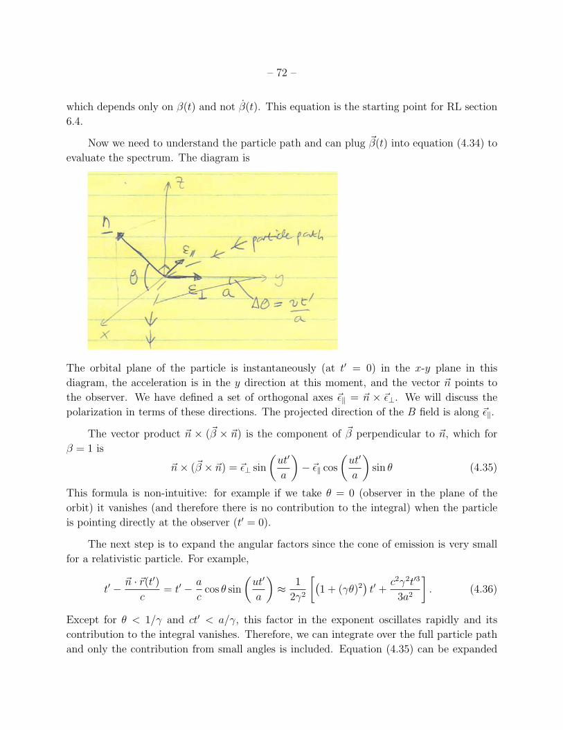
– 72 –

which depends only on �(t) and not �(t). This equation is the starting point for RL section

6.4.

Now we need to understand the particle path and can plug ~�(t) into equation (4.34) to

evaluate the spectrum. The diagram is

The orbital plane of the particle is instantaneously (at t0 = 0) in the x-y plane in this

diagram, the acceleration is in the y direction at this moment, and the vector ~n points to

the observer. We have defined a set of orthogonal axes ~✏k = ~n ⇥ ~✏?. We will discuss the

polarization in terms of these directions. The projected direction of the B field is along ~✏k.

The vector product ~n ⇥ (~� ⇥ ~n) is the component of ~� perpendicular to ~n, which for

� = 1 is

~n⇥ (~� ⇥ ~n) = ~✏? sin

✓ut0

a

◆� ~✏k cos

✓ut0

a

◆sin ✓ (4.35)

This formula is non-intuitive: for example if we take ✓ = 0 (observer in the plane of the

orbit) it vanishes (and therefore there is no contribution to the integral) when the particle

is pointing directly at the observer (t0 = 0).

The next step is to expand the angular factors since the cone of emission is very small

for a relativistic particle. For example,

t0 �~n · ~r(t0)

c= t0 �

a

ccos ✓ sin

✓ut0

a

◆⇡

1

2�2

�1 + (�✓)2

�t0 +

c2�2t03

3a2

�. (4.36)

Except for ✓ < 1/� and ct0 < a/�, this factor in the exponent oscillates rapidly and its

contribution to the integral vanishes. Therefore, we can integrate over the full particle path

and only the contribution from small angles is included. Equation (4.35) can be expanded

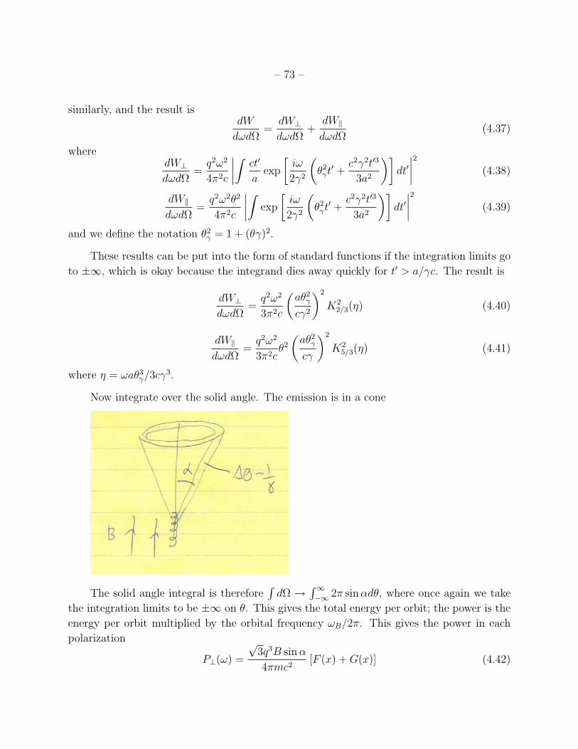
– 73 –

similarly, and the result isdW

d!d⌦=

dW?

d!d⌦+

dWk

d!d⌦(4.37)

wheredW?

d!d⌦=

q2!2

4⇡2c

����Z

ct0

aexp

i!

2�2

✓✓2

�t0 +

c2�2t03

3a2

◆�dt0����2

(4.38)

dWk

d!d⌦=

q2!2✓2

4⇡2c

����Z

exp

i!

2�2

✓✓2

�t0 +

c2�2t03

3a2

◆�dt0����2

(4.39)

and we define the notation ✓2

� = 1 + (✓�)2.

These results can be put into the form of standard functions if the integration limits go

to ±1, which is okay because the integrand dies away quickly for t0 > a/�c. The result is

dW?

d!d⌦=

q2!2

3⇡2c

✓a✓2

�

c�2

◆2

K2

2/3

(⌘) (4.40)

dWk

d!d⌦=

q2!2

3⇡2c✓2

✓a✓2

�

c�

◆2

K2

5/3

(⌘) (4.41)

where ⌘ = !a✓3

�/3c�3.

Now integrate over the solid angle. The emission is in a cone

The solid angle integral is thereforeR

d⌦ !R1�1 2⇡ sin↵d✓, where once again we take

the integration limits to be ±1 on ✓. This gives the total energy per orbit; the power is the

energy per orbit multiplied by the orbital frequency !B/2⇡. This gives the power in each

polarization

P?(!) =

p

3q3B sin↵

4⇡mc2

[F (x) + G(x)] (4.42)

– 74 –

Pk(!) =

p

3q3B sin↵

4⇡mc2

[F (x)�G(x)] (4.43)

where x = !/!c, F (x) = xR1

xd⇠K

5/3

(⇠) and G(x) = xK2/3

(x). The total power in both

polarizations is

P (!) =

p

3q3B sin↵

2⇡mc2

F (x). (4.44)

The following integrals of F (x) and G(x) are useful

Z 1

0

xµF (x)dx =2µ+1

µ + 2�

✓µ

2+

7

3

◆�

✓µ

2+

2

3

◆(4.45)

Z 1

0

xµG(x)dx = 2µ�

✓µ

2+

4

3

◆�

✓µ

2+

2

3

◆. (4.46)

For a power-law distribution of electron energies N(�) = N(�1

)(�/�1

)�p, the frequency

spectrum is given bydP

dV d!=

Z �2

�1

N(�)d�dP

d!. (4.47)

For �2

� �1

and p > 1, the number density of electrons is ne = N(�1

)�1

/(p� 1), giving

dP

dV d!=

p

3q3B sin↵

2⇡mc2

(p� 1)ne

�1

Z ✓�

�1

◆�p

F (x)d�. (4.48)

Now as we discussed earlier, changing integration variable from � to

x =!

!c

= ��2

✓2!mc

3eB sin↵

◆(4.49)

givesdP

dV d!/ B(p+1)/2!�(p�1)/2. (4.50)

4.6. Important features of synchrotron radiation and some applications

Let’s briefly highlight here some important aspects of synchrotron radiation. These are

worked out in more detail in HW4.

• Polarization. One of the distinguishing features of synchrotron radiation is that it

is strongly-polarized. For cyclotron emission, this is straightforward to see from the

following diagram

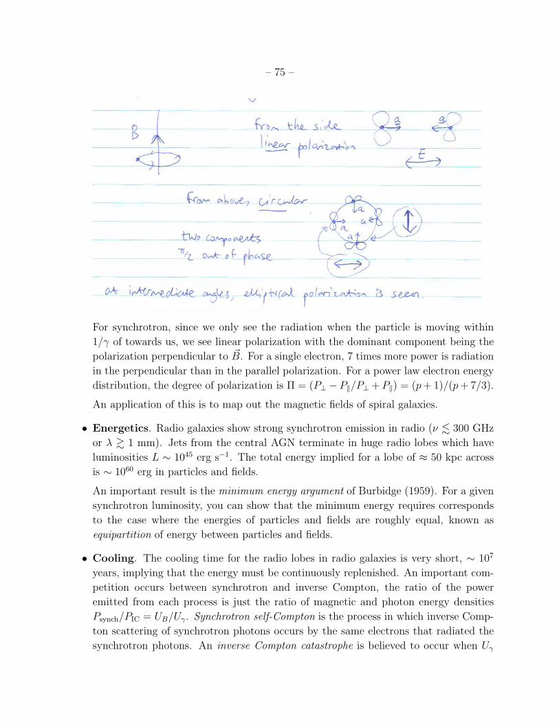
– 75 –

For synchrotron, since we only see the radiation when the particle is moving within

1/� of towards us, we see linear polarization with the dominant component being the

polarization perpendicular to ~B. For a single electron, 7 times more power is radiation

in the perpendicular than in the parallel polarization. For a power law electron energy

distribution, the degree of polarization is ⇧ = (P?� Pk/P? + Pk) = (p + 1)/(p + 7/3).

An application of this is to map out the magnetic fields of spiral galaxies.

• Energetics. Radio galaxies show strong synchrotron emission in radio (⌫ . 300 GHz

or � & 1 mm). Jets from the central AGN terminate in huge radio lobes which have

luminosities L ⇠ 1045 erg s�1. The total energy implied for a lobe of ⇡ 50 kpc across

is ⇠ 1060 erg in particles and fields.

An important result is the minimum energy argument of Burbidge (1959). For a given

synchrotron luminosity, you can show that the minimum energy requires corresponds

to the case where the energies of particles and fields are roughly equal, known as

equipartition of energy between particles and fields.

• Cooling. The cooling time for the radio lobes in radio galaxies is very short, ⇠ 107

years, implying that the energy must be continuously replenished. An important com-

petition occurs between synchrotron and inverse Compton, the ratio of the power

emitted from each process is just the ratio of magnetic and photon energy densities

Psynch

/PIC

= UB/U�. Synchrotron self-Compton is the process in which inverse Comp-

ton scattering of synchrotron photons occurs by the same electrons that radiated the

synchrotron photons. An inverse Compton catastrophe is believed to occur when U�

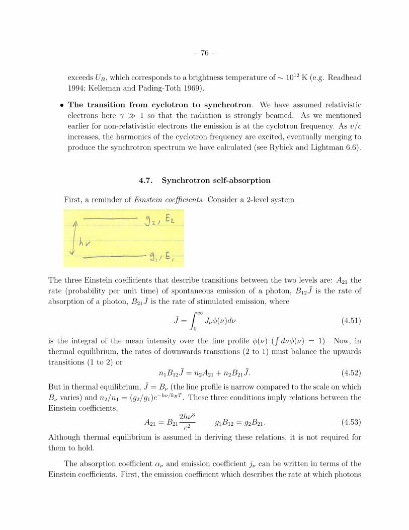
– 76 –

exceeds UB, which corresponds to a brightness temperature of ⇠ 1012 K (e.g. Readhead

1994; Kelleman and Pading-Toth 1969).

• The transition from cyclotron to synchrotron. We have assumed relativistic

electrons here � � 1 so that the radiation is strongly beamed. As we mentioned

earlier for non-relativistic electrons the emission is at the cyclotron frequency. As v/c

increases, the harmonics of the cyclotron frequency are excited, eventually merging to

produce the synchrotron spectrum we have calculated (see Rybick and Lightman 6.6).

4.7. Synchrotron self-absorption

First, a reminder of Einstein coe�cients. Consider a 2-level system

The three Einstein coe�cients that describe transitions between the two levels are: A21

the

rate (probability per unit time) of spontaneous emission of a photon, B12

J is the rate of

absorption of a photon, B21

J is the rate of stimulated emission, where

J =

Z 1

0

J⌫�(⌫)d⌫ (4.51)

is the integral of the mean intensity over the line profile �(⌫) (R

d⌫�(⌫) = 1). Now, in

thermal equilibrium, the rates of downwards transitions (2 to 1) must balance the upwards

transitions (1 to 2) or

n1

B12

J = n2

A21

+ n2

B21

J . (4.52)

But in thermal equilibrium, J = B⌫ (the line profile is narrow compared to the scale on which

B⌫ varies) and n2

/n1

= (g2

/g1

)e�h⌫/kBT . These three conditions imply relations between the

Einstein coe�cients,

A21

= B21

2h⌫3

c2

g1

B12

= g2

B21

. (4.53)

Although thermal equilibrium is assumed in deriving these relations, it is not required for

them to hold.

The absorption coe�cient ↵⌫ and emission coe�cient j⌫ can be written in terms of the

Einstein coe�cients. First, the emission coe�cient which describes the rate at which photons

– 77 –

are added to the radiation field independent of the incident radiation we relate to A21

j⌫ =h⌫

4⇡n

2

A21

�(⌫). (4.54)

Since the stimulated emission is proportional to J , we include it in the absorption coe�cient

as a negative absorption term. The net absorption is

n1

B12

J

✓1�

n2

n1

B21

B12

◆= n

1

B12

J�1� e�h⌫/kBT

�, (4.55)

where in the last step we use the level populations in thermal equilibrium. Note that this

does not require full thermal equilibrium to be valid, but only LTE; we assume that the level

densities are thermally-populated but the matter does not have to be in equilibrium with

the photons. Therefore it is often a good assumption. The term in brackets is referred to

as the correction for stimulated emission. We have seen it previously in the expression for

free-free absorption. The absorption coe�cient is then

↵⌫ =h⌫

4⇡n

1

B12

�(⌫)(1� e�h⌫/kBT ). (4.56)

Now we can apply these ideas to synchrotron absorption. The idea is to use the Einstein

relations to obtain the synchrotron absorption coe�cient from the emission coe�cient that

we have already calculated. The main di↵erence is that rather than a two-level system,

in this case we must consider transitions between states in the continuum. The emission

coe�cient can be written

j⌫ =1

4⇡

Zd3~pf(p)P⌫(p) (4.57)

where f(p) is the density of states as a function of electron momentum p, and P⌫(p) is

the power emitted at frequency ⌫ by an electron with momentum p (something we have

calculated in previous sections). Then applying the Einstein relations, we get the absorption

coe�cient

↵⌫ =c2

8⇡h⌫3

Zd3~p [f(~p?)� f(~p)] P⌫(p) (4.58)

where p? is the electron momentum corresponding to an energy ✏+ h⌫.

As a check, we can put in a thermal (Maxwell-Boltzmann) distribution for the electron

distribution, f(p) = Ce�✏/kBT . Then f(p?) = Ce�✏/kBT eh⌫/kBT , which gives

↵⌫ =c2

2h⌫3

(eh⌫/kBT� 1)

1

4⇡

Zd3~pf(p)P⌫(p) =

j⌫

B⌫

. (4.59)

And so we see that we recover Kircho↵’s law j⌫ = ↵⌫B⌫ . You may recall that we used

Kircho↵’s law directly to get the free-free absorption coe�cient from the free-free emissivity.

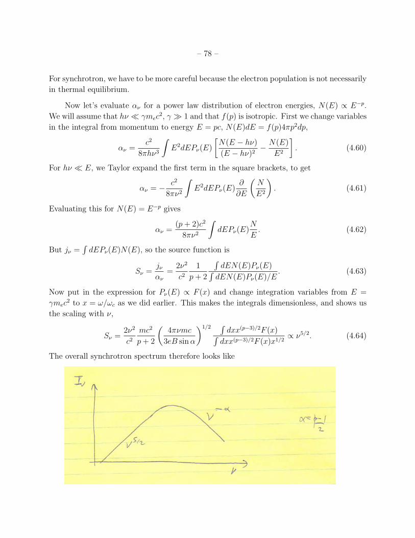
– 78 –

For synchrotron, we have to be more careful because the electron population is not necessarily

in thermal equilibrium.

Now let’s evaluate ↵⌫ for a power law distribution of electron energies, N(E) / E�p.

We will assume that h⌫ ⌧ �mec2, � � 1 and that f(p) is isotropic. First we change variables

in the integral from momentum to energy E = pc, N(E)dE = f(p)4⇡p2dp,

↵⌫ =c2

8⇡h⌫3

ZE2dEP⌫(E)

N(E � h⌫)

(E � h⌫)2

�

N(E)

E2

�. (4.60)

For h⌫ ⌧ E, we Taylor expand the first term in the square brackets, to get

↵⌫ = �c2

8⇡⌫2

ZE2dEP⌫(E)

@

@E

✓N

E2

◆. (4.61)

Evaluating this for N(E) = E�p gives

↵⌫ =(p + 2)c2

8⇡⌫2

ZdEP⌫(E)

N

E. (4.62)

But j⌫ =R

dEP⌫(E)N(E), so the source function is

S⌫ =j⌫

↵⌫

=2⌫2

c2

1

p + 2

RdEN(E)P⌫(E)R

dEN(E)P⌫(E)/E. (4.63)

Now put in the expression for P⌫(E) / F (x) and change integration variables from E =

�mec2 to x = !/!c as we did earlier. This makes the integrals dimensionless, and shows us

the scaling with ⌫,

S⌫ =2⌫2

c2

mc2

p + 2

✓4⇡⌫mc

3eB sin↵

◆1/2

Rdxx(p�3)/2F (x)R

dxx(p�3)/2F (x)x1/2

/ ⌫5/2. (4.64)

The overall synchrotron spectrum therefore looks like

– 79 –

turning over from the optically thin scaling / ⌫�(p�1)/2 at high frequency to / ⌫5/2 at low

frequencies where the source becomes optically thick to synchrotron self-absorption.

By comparing this with S⌫ = (2⌫2/c2)kBTb, we see that the brightness temperature is

kBTb

mec2

=

!

3

2

eBmec

sin↵

!1/2⇢

1

p + 2

Rdxx(p�3)/2F (x)R

dxx(p�3)/2F (x)x1/2

�. (4.65)

If we look at frequency !, that emission is primarily coming from electrons with energy �!

such that ! = !c = �2

!(3eB/2mec) sin↵, so we can write

kBTb

mec2

= �!

⇢1

p + 2

Rdxx(p�3)/2F (x)R

dxx(p�3)/2F (x)x1/2

�. (4.66)

This then gives us a way to think of the self-absorbed spectrum. At each frequency, we

calculate the � of the electrons that radiate the peak of their spectrum at that frequency,

i.e. we calculate �!. The brightness temperature at that frequency is then given by kBT ⇡

�!mec2

/ ⌫1/2 and therefore S⌫ / ⌫5/2. This is the back of the envelope understanding of

the spectrum that is often given in the books.

Summary and Further Reading

Here are the main ideas and results that we covered in this part of the course:

• Cyclotron radiation from non-relativistic electrons. Cyclotron frequency !c = eB/mec =,

or fc = 2.8 MHz (B/G).

• Synchrotron. Relativistic gyration frequency !B = eB/�mec. Power radiated per

electron P = (4/3)�2�2�T cUB. Distinction between “emitted” and “received” power.

Angular distribution of radiation from a relativistic charge – beaming into angle 1/�.

Characteristic frequency of radiation !c = (3/2)�3!B sin↵ (roughly 1/pulse duration).

Broad spectrum / x1/3 (x = !/!c ⌧ 1) or x1/2e�x (x � 1), peaks at x ⇡ 0.3. Exact

form

P?(!) =

p

3e3B sin↵

4⇡mec2

[F (x) + G(x)] P?(!) =

p

3e3B sin↵

4⇡mec2

[F (x)�G(x)]

• For a power law distribution of electrons, dP/dV d! / B(p+1)/2!�(p�1)/2. Typically,

p ⇡ 2.5 giving ↵ = (p� 1)/2 ⇡ 0.7.

– 80 –

• Einstein coe�cients. A21

= B21

(2h⌫3/c2), g1

B12

= g2

B21

. Correction to absorption co-

e�cient for stimulated emission. j⌫ = (h⌫/4⇡)n2

A21

�(⌫), ↵⌫ = (h⌫/4⇡)n1

B12

�(⌫)(1�

e�h⌫/kBT ).

• Synchrotron self-absorption. S⌫ / ⌫5/2, kBTb ⇡ �mec2 where � is such that !c = !.

• Important features of synchrotron radiation. Polarization as a characteristic feature of

synchrotron radiation. Minimum energy argument. Cooling timescales for synchrotron

and inverse Compton. The inverse Compton catastrophe. Application to radio galax-

ies, magnetic fields of spiral galaxies.

Reading

• Synchrotron derivation: RL section 6.4, Jackson 14.6, Longair volume 2. Westfold

(1959) ApJ.

• Minimum energy argument, Burbidge 1959. Inverse Compton catastrophe, Readhead

1994, Kelleman & Pauliny-Toth 1969.

– 81 –

5. Fermi Acceleration and Plasma E↵ects

These are notes for part five of PHYS 642 Radiative Processes in Astrophysics. We

discuss two distinct topics: the origin of power-law distributions of particle energy, in partic-

ular Fermi acceleration in strong shocks as a generic origin of power-law distributions, and

propagation of electromagnetic waves through plasma, including the e↵ects of dispersion and

Faraday rotation.

5.1. General way to make a power law spectrum of particle energies

A characteristic spectral index for synchrotron is ↵ ⇡ 0.7 (F⌫ / ⌫�0.7) which implies

p ⇡ 2.5 (N(�) / ��2.5) (recall that ↵ = (p � 1)/2). This raises the question of why the

electron distribution is a power law and in particular why p has this value.

We already have a clue as to how get a power law from our discussion of Compton

scattering by optically thin relativistic electrons (see also Rybicki and Lightman 7.5). There,

the photon energy increased by the same fractional amount �✏/✏ on each scattering, but

each subsequent scattering is less likely by a factor of the optical depth ⌧ . The resulting

spectrum is a power law.

Here the idea is similar: imagine a scattering process for particles in which the energy

of the particle changes by �✏/✏ = B on average, but there is also a probability per collision

that the particles escape Pesc

. If the mean time between collisions is tc, then the particle

energy obeys d✏/dt = ✏B/tc or ✏ = ✏0

eBt/tc . On the other hand, the number of particles drops

according to dN/dt = �NPesc

/tc so that N = N0

e�tPesc

/tc . Dividing these distributions gives

the energy distribution

dN

d✏=

dN

dt

dt

d✏/ e�P

esc

t/tce�Bt/tc/ e�(Bt/tc)(1+P

esc

/B)

/

✓✏

✏0

◆�(1+Pesc

/B)

. (5.1)

A power law distribution of energies is the result, with index p = 1 + Pesc

/B.

5.2. Second order Fermi acceleration

Originally, Fermi suggested a mechanism in which particles would be accelerated on

colliding from moving clouds of gas. For example, consider the collision of a particle with a

cloud moving with velocity V to the right. The particle travels to the left with velocity v

and makes an angle ✓ with respect to the normal to the surface.

– 82 –

The way to analyze this collision is to move into the frame of the cloud. The cloud

is much more massive than the particle and so in that frame we can think of the particle

reversing it’s momentum but not changing its energy. The incoming energy and momentum

in the rest frame of the cloud are E 0 = �V (E + pV cos ✓) and p0x = �V (p cos ✓ + V E/c2),

where �V refers to � calculated using the velocity V of the cloud. In the collision, the energy

is unchanged, but the x-component of momentum reverses. Now transforming back, the

energy of the particle post-collision in the original frame is E 00 = �V (E 0 + V p0x) or

E 00 = E�2

V

1 + 2

pV

Ecos ✓ +

V 2

c2

�(5.2)

or to second order in V/c,�E

E=

2vV

c2

cos ✓ + 2

✓V

c

◆2

. (5.3)

To average over angles, we note that the rate of encounters of the particle with a cloud

depends on whether the collision is a trailing collision or head-on collision. Specifically, the

rate of encounters is / 1 + (V/c) cos ✓). Therefore

h

�E

Ei =

R1

�1

dµ(1 + (V/c)µ)(2(V/c)2 + (2V v/c2)µ)R

1

�1

dµ(1 + (V/c)µ)(5.4)

which for v = c is h�E/Ei = (8/3)(V/c)2, second order in V/c.

The fact that the acceleration is only second order makes it ine�cient, but perhaps a

more important objection to this mechanism is that the values of Pesc

and B, and therefore

the power law index p, are not expected to be generic. They would presumably depend on

the environment that the particle happens to find itself in.

5.3. First order Fermi acceleration by strong shocks

This is a mechanism in which particles scatter back and forth across a shock. Consider

a strong shock9 in gas with � = 5/3. You may recall that in the frame of the shock, the

incoming supersonic matter is slowed by the shock to a speed us/4, and compressed by a

factor of 4 (⇢2

= 4⇢1

). Here is a picture of the shock in the lab frame and in the frame

moving with the shock:

9These results come from applying conservation of mass, momentum and energy across the shock. Massconservation is ⇢1u1 = ⇢2u2. For a strong shock, the force balance is P2 ⇡ ⇢1u

21.

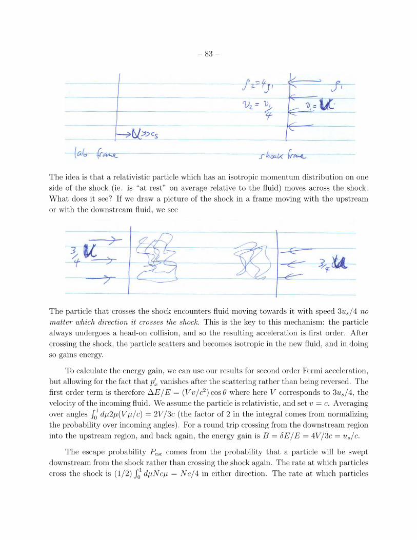
– 83 –

The idea is that a relativistic particle which has an isotropic momentum distribution on one

side of the shock (ie. is “at rest” on average relative to the fluid) moves across the shock.

What does it see? If we draw a picture of the shock in a frame moving with the upstream

or with the downstream fluid, we see

The particle that crosses the shock encounters fluid moving towards it with speed 3us/4 no

matter which direction it crosses the shock. This is the key to this mechanism: the particle

always undergoes a head-on collision, and so the resulting acceleration is first order. After

crossing the shock, the particle scatters and becomes isotropic in the new fluid, and in doing

so gains energy.

To calculate the energy gain, we can use our results for second order Fermi acceleration,

but allowing for the fact that p0x vanishes after the scattering rather than being reversed. The

first order term is therefore �E/E = (V v/c2) cos ✓ where here V corresponds to 3us/4, the

velocity of the incoming fluid. We assume the particle is relativistic, and set v = c. Averaging

over anglesR

1

0

dµ2µ(V µ/c) = 2V/3c (the factor of 2 in the integral comes from normalizing

the probability over incoming angles). For a round trip crossing from the downstream region

into the upstream region, and back again, the energy gain is B = �E/E = 4V/3c = us/c.

The escape probability Pesc

comes from the probability that a particle will be swept

downstream from the shock rather than crossing the shock again. The rate at which particles

cross the shock is (1/2)R

1

0

dµNcµ = Nc/4 in either direction. The rate at which particles

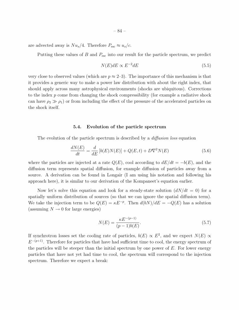
– 84 –

are advected away is Nus/4. Therefore Pesc

⇡ us/c.

Putting these values of B and Pesc

into our result for the particle spectrum, we predict

N(E)dE / E�2dE (5.5)

very close to observed values (which are p ⇡ 2–3). The importance of this mechanism is that

it provides a generic way to make a power law distribution with about the right index, that

should apply across many astrophysical environments (shocks are ubiquitous). Corrections

to the index p come from changing the shock compressibility (for example a radiative shock

can have ⇢2

� ⇢1

) or from including the e↵ect of the pressure of the accelerated particles on

the shock itself.

5.4. Evolution of the particle spectrum

The evolution of the particle spectrum is described by a di↵usion loss equation

dN(E)

dt=

d

dE[b(E)N(E)] + Q(E, t) + Dr2N(E) (5.6)

where the particles are injected at a rate Q(E), cool according to dE/dt = �b(E), and the

di↵usion term represents spatial di↵usion, for example di↵usion of particles away from a

source. A derivation can be found in Longair (I am using his notation and following his

approach here), it is similar to our derivation of the Kompaneet’s equation earlier.

Now let’s solve this equation and look for a steady-state solution (dN/dt = 0) for a

spatially uniform distribution of sources (so that we can ignore the spatial di↵usion term).

We take the injection term to be Q(E) = E�p. Then d(bN)/dE = �Q(E) has a solution

(assuming N ! 0 for large energies)

N(E) =E�(p�1)

(p� 1)b(E). (5.7)

If synchrotron losses set the cooling rate of particles, b(E) / E2, and we expect N(E) /

E�(p+1). Therefore for particles that have had su�cient time to cool, the energy spectrum of

the particles will be steeper than the initial spectrum by one power of E. For lower energy

particles that have not yet had time to cool, the spectrum will correspond to the injection

spectrum. Therefore we expect a break:

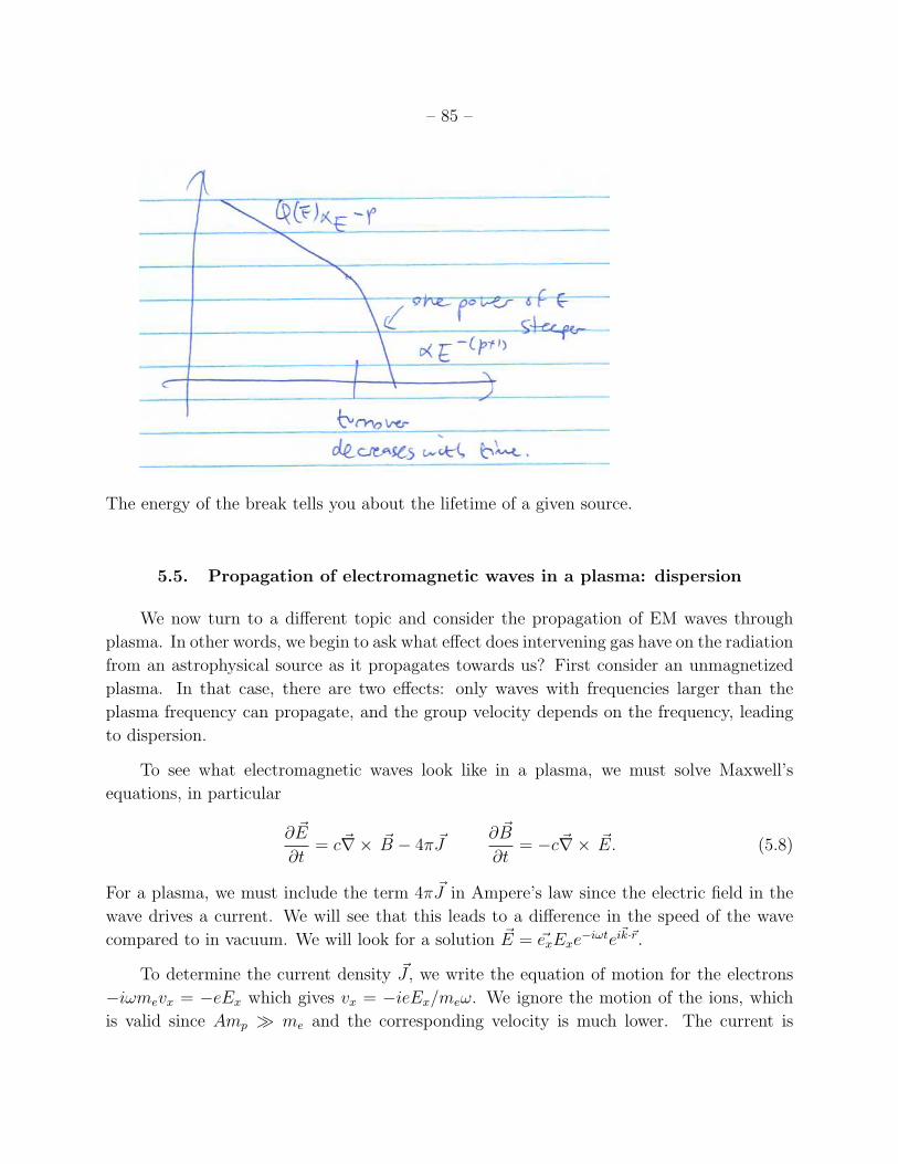
– 85 –

The energy of the break tells you about the lifetime of a given source.

5.5. Propagation of electromagnetic waves in a plasma: dispersion

We now turn to a di↵erent topic and consider the propagation of EM waves through

plasma. In other words, we begin to ask what e↵ect does intervening gas have on the radiation

from an astrophysical source as it propagates towards us? First consider an unmagnetized

plasma. In that case, there are two e↵ects: only waves with frequencies larger than the

plasma frequency can propagate, and the group velocity depends on the frequency, leading

to dispersion.

To see what electromagnetic waves look like in a plasma, we must solve Maxwell’s

equations, in particular

@ ~E

@t= c~r⇥ ~B � 4⇡ ~J

@ ~B

@t= �c~r⇥ ~E. (5.8)

For a plasma, we must include the term 4⇡ ~J in Ampere’s law since the electric field in the

wave drives a current. We will see that this leads to a di↵erence in the speed of the wave

compared to in vacuum. We will look for a solution ~E = ~exExe�i!tei~k·~r.

To determine the current density ~J , we write the equation of motion for the electrons

�i!mevx = �eEx which gives vx = �ieEx/me!. We ignore the motion of the ions, which

is valid since Amp � me and the corresponding velocity is much lower. The current is

– 86 –

~J = �ene~ve, or

Jx = inee

2

me!Ex. (5.9)

Note that the current and electric field are ⇡/2 out of phase, and therefore h ~J ·

~Ei = 0: there

is no net work done on the plasma by the wave. Therefore the wave propagates without

dissipation.

The next step is to write ~r⇥ ~B / ~E using the fact that ~J / ~E,

i~k ⇥ ~B =4⇡ ~J

c�

i! ~E

c= �

i!

c✏ ~E (5.10)

where we have introduced the dielectric constant of the plasma ✏,

✏ = 1�4⇡nee

2

me

1

!2

= 1�!2

p

!2

(5.11)

which defines the plasma frequency !2

p = 4⇡nee2/me.

Now we solve for the disperson relation for the wave. Maxwell’s equations are

i~k ⇥ ~B = �i!

c✏ ~E i~k ⇥ ~E =

i!

c~B (5.12)

which gives

~k ⇥ (~k ⇥ ~E) = �⇣!

c

⌘2

✏ ~E (5.13)

which is the dispersion relation for a transverse wave (~k. ~E = 0) with !2 = c2k2/✏, or

k =1

c

q!2

� !2

p. (5.14)

We see that for ! > !p, k is real and the wave propagates, but for ! < !p, k is imaginary

and the wave evanesces. Physically, what’s going on is that at high frequency, the electrons

don’t have time to accelerate, and therefore the current is small and has little e↵ect on the

wave. At low frequencies, a significant current can build up during a wave period that acts

to “short out” the wave (recall that there is no static electric field inside a conductor, ie. the

electric field vanishes in the limit ! ! 0). Putting in numbers, we get a useful formula

fp =!p

2⇡= 9.0 kHz

⇣ ne

cm�3

⌘1/2

. (5.15)

A terrestrial application is to the Earth’s ionsphere in which ne ⇠ 104

� 105 cm�3 and radio

waves with frequencies below a few MHz are reflected back towards the Earth’s surface.

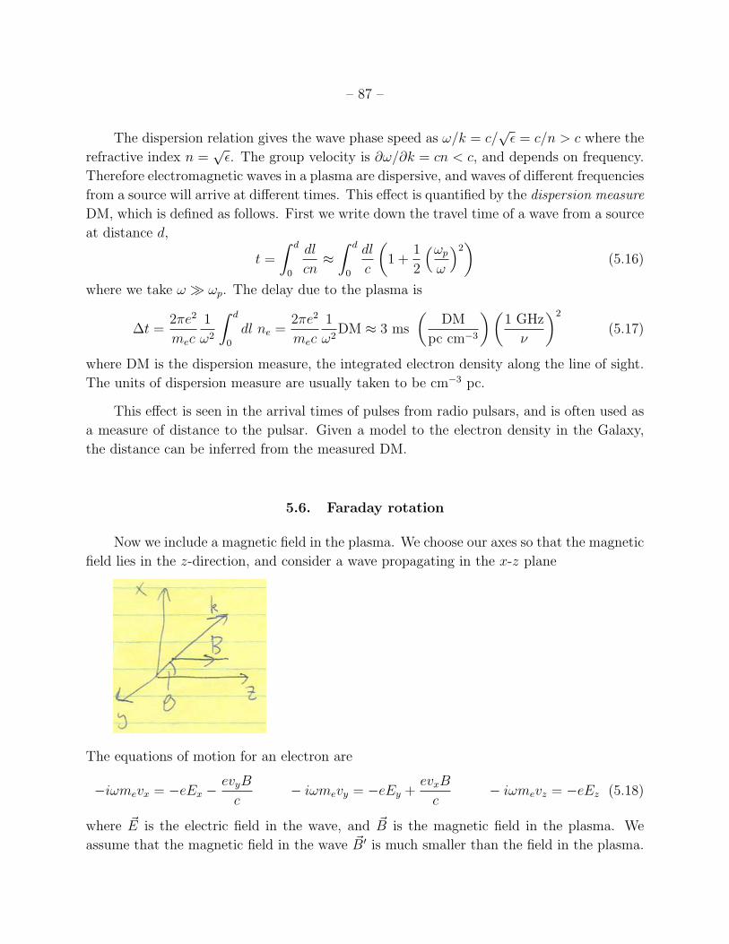
– 87 –

The dispersion relation gives the wave phase speed as !/k = c/p

✏ = c/n > c where the

refractive index n =p

✏. The group velocity is @!/@k = cn < c, and depends on frequency.

Therefore electromagnetic waves in a plasma are dispersive, and waves of di↵erent frequencies

from a source will arrive at di↵erent times. This e↵ect is quantified by the dispersion measure

DM, which is defined as follows. First we write down the travel time of a wave from a source

at distance d,

t =

Z d

0

dl

cn⇡

Z d

0

dl

c

✓1 +

1

2

⇣!p

!

⌘2

◆(5.16)

where we take ! � !p. The delay due to the plasma is

�t =2⇡e2

mec

1

!2

Z d

0

dl ne =2⇡e2

mec

1

!2

DM ⇡ 3 ms

✓DM

pc cm�3

◆✓1 GHz

⌫

◆2

(5.17)

where DM is the dispersion measure, the integrated electron density along the line of sight.

The units of dispersion measure are usually taken to be cm�3 pc.

This e↵ect is seen in the arrival times of pulses from radio pulsars, and is often used as

a measure of distance to the pulsar. Given a model to the electron density in the Galaxy,

the distance can be inferred from the measured DM.

5.6. Faraday rotation

Now we include a magnetic field in the plasma. We choose our axes so that the magnetic

field lies in the z-direction, and consider a wave propagating in the x-z plane

The equations of motion for an electron are

�i!mevx = �eEx �evyB

c� i!mevy = �eEy +

evxB

c� i!mevz = �eEz (5.18)

where ~E is the electric field in the wave, and ~B is the magnetic field in the plasma. We

assume that the magnetic field in the wave ~B0 is much smaller than the field in the plasma.

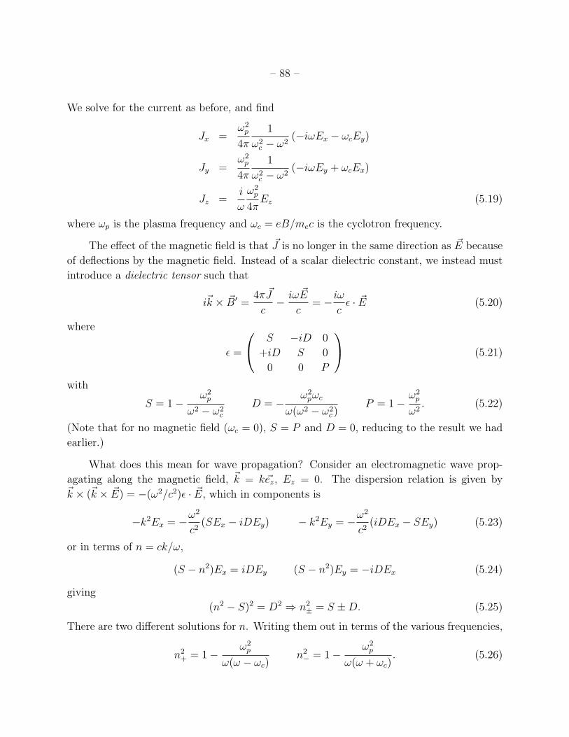
– 88 –

We solve for the current as before, and find

Jx =!2

p

4⇡

1

!2

c � !2

(�i!Ex � !cEy)

Jy =!2

p

4⇡

1

!2

c � !2

(�i!Ey + !cEx)

Jz =i

!

!2

p

4⇡Ez (5.19)

where !p is the plasma frequency and !c = eB/mec is the cyclotron frequency.

The e↵ect of the magnetic field is that ~J is no longer in the same direction as ~E because

of deflections by the magnetic field. Instead of a scalar dielectric constant, we instead must

introduce a dielectric tensor such that

i~k ⇥ ~B0 =4⇡ ~J

c�

i! ~E

c= �

i!

c✏ · ~E (5.20)

where

✏ =

0

@S �iD 0

+iD S 0

0 0 P

1

A (5.21)

with

S = 1�!2

p

!2

� !2

c

D = �!2

p!c

!(!2

� !2

c )P = 1�

!2

p

!2

. (5.22)

(Note that for no magnetic field (!c = 0), S = P and D = 0, reducing to the result we had

earlier.)

What does this mean for wave propagation? Consider an electromagnetic wave prop-

agating along the magnetic field, ~k = k~ez, Ez = 0. The dispersion relation is given by~k ⇥ (~k ⇥ ~E) = �(!2/c2)✏ · ~E, which in components is

�k2Ex = �!2

c2

(SEx � iDEy) � k2Ey = �!2

c2

(iDEx � SEy) (5.23)

or in terms of n = ck/!,

(S � n2)Ex = iDEy (S � n2)Ey = �iDEx (5.24)

giving

(n2

� S)2 = D2

) n2

± = S ± D. (5.25)

There are two di↵erent solutions for n. Writing them out in terms of the various frequencies,

n2

+

= 1�!2

p

!(! � !c)n2

� = 1�!2

p

!(! + !c). (5.26)

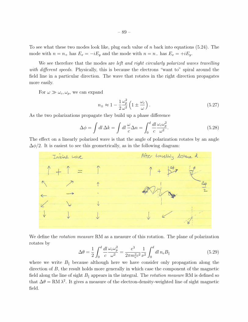
– 89 –

To see what these two modes look like, plug each value of n back into equations (5.24). The

mode with n = n+

has Ex = �iEy and the mode with n = n� has Ex = +iEy.

We see therefore that the modes are left and right circularly polarized waves travelling

with di↵erent speeds. Physically, this is because the electrons “want to” spiral around the

field line in a particular direction. The wave that rotates in the right direction propagates

more easily.

For ! � !c,!p, we can expand

n± ⇡ 1�1

2

!2

p

!2

⇣1 ±

!c

!

⌘. (5.27)

As the two polarizations propagate they build up a phase di↵erence

�� =

Zdl �k =

Zdl!

c�n =

Z d

0

dl

c

!c!2

p

!2

. (5.28)

The e↵ect on a linearly polarized wave is that the angle of polarization rotates by an angle

��/2. It is easiest to see this geometrically, as in the following diagram:

We define the rotation measure RM as a measure of this rotation. The plane of polarization

rotates by

�✓ =1

2

Z d

0

dl

c

!c!2

p

!2

=e3

2⇡m2

ec2

1

⌫2

Z d

0

dl neBk (5.29)

where we write Bk because although here we have consider only propagation along the

direction of B, the result holds more generally in which case the component of the magnetic

field along the line of sight Bk appears in the integral. The rotation measure RM is defined so

that �✓ = RM�2. It gives a measure of the electron-density-weighted line of sight magnetic

field.

– 90 –

Summary and Further Reading

Here are the main ideas and results that we covered in this part of the course:

• Origin and evolution of electron spectrum. How to generate a power law energy dis-

tribution. Fermi acceleration. Scattering across a strong shock front gives p ⇡ 2. A

break in the electron spectrum indicates the energy where the cooling time equals the

age of the population.

• Electromagnetic waves in a plasma. Plasma frequency !2

p = 4⇡nee2/me, or fp =

9 kHz n1/2

e . Refractive index n2 = 1 � !2

p/!2. Dispersion �t = (2⇡e2/mec)(DM/!2),

where DM =R

ne dl. Faraday rotation. Rotation measure �✓ = RM�2, RM /RneBk dl.

Reading

• Electron spectrum: good discussions are in Longair and Kulsrud 12.7.

• Electron model for Galaxy used to interpret DM measurements: Taylor & Cordes 1993

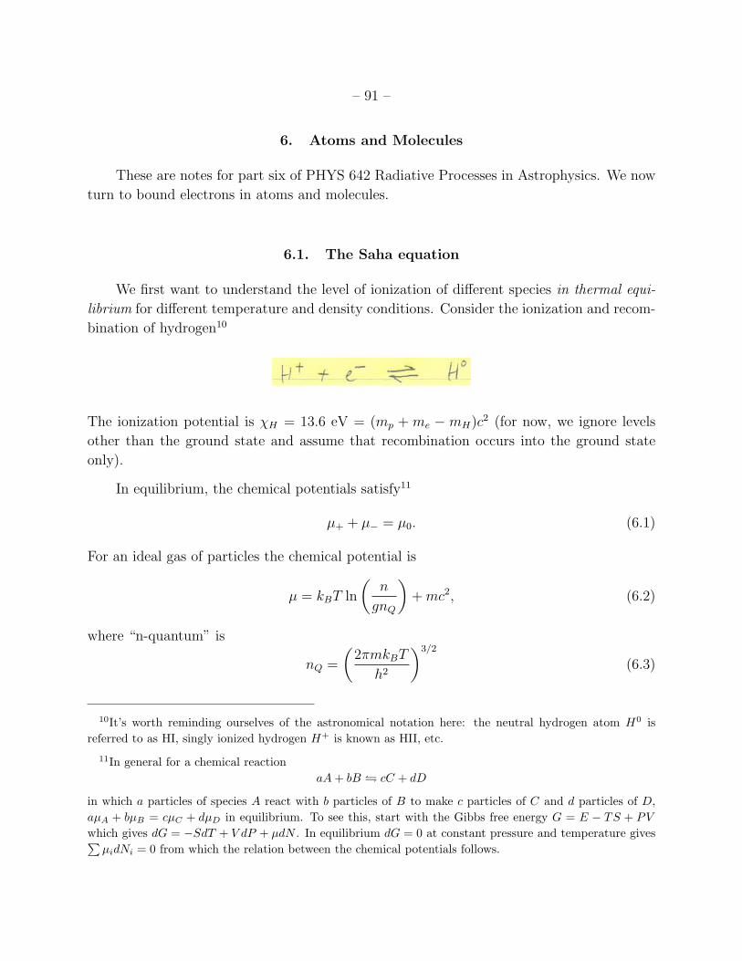
– 91 –

6. Atoms and Molecules

These are notes for part six of PHYS 642 Radiative Processes in Astrophysics. We now

turn to bound electrons in atoms and molecules.

6.1. The Saha equation

We first want to understand the level of ionization of di↵erent species in thermal equi-

librium for di↵erent temperature and density conditions. Consider the ionization and recom-

bination of hydrogen10

The ionization potential is �H = 13.6 eV = (mp + me � mH)c2 (for now, we ignore levels

other than the ground state and assume that recombination occurs into the ground state

only).

In equilibrium, the chemical potentials satisfy11

µ+

+ µ� = µ0

. (6.1)

For an ideal gas of particles the chemical potential is

µ = kBT ln

✓n

gnQ

◆+ mc2, (6.2)

where “n-quantum” is

nQ =

✓2⇡mkBT

h2

◆3/2

(6.3)

10It’s worth reminding ourselves of the astronomical notation here: the neutral hydrogen atom H0 isreferred to as HI, singly ionized hydrogen H+ is known as HII, etc.

11In general for a chemical reactionaA + bB ↵ cC + dD

in which a particles of species A react with b particles of B to make c particles of C and d particles of D,aµ

A

+ bµB

= cµC

+ dµD

in equilibrium. To see this, start with the Gibbs free energy G = E � TS + PV

which gives dG = �SdT + V dP + µdN . In equilibrium dG = 0 at constant pressure and temperature givesPµ

i

dNi

= 0 from which the relation between the chemical potentials follows.

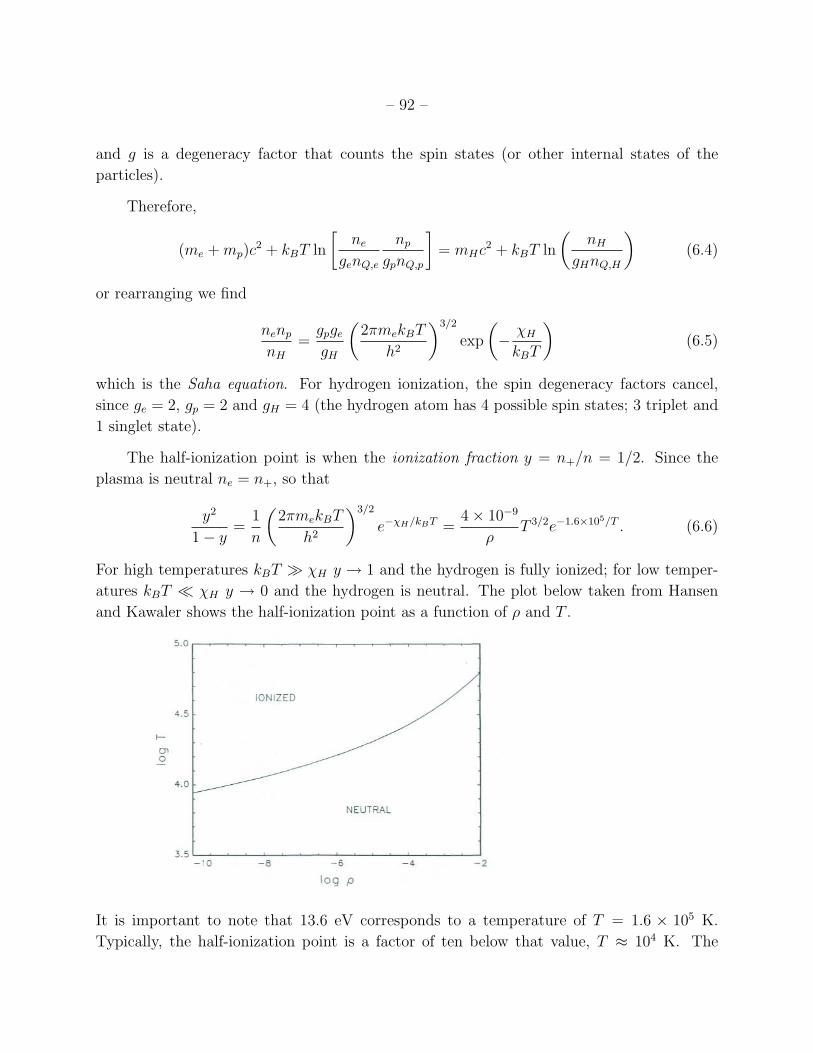
– 92 –

and g is a degeneracy factor that counts the spin states (or other internal states of the

particles).

Therefore,

(me + mp)c2 + kBT ln

ne

genQ,e

np

gpnQ,p

�= mHc2 + kBT ln

✓nH

gHnQ,H

◆(6.4)

or rearranging we find

nenp

nH

=gpge

gH

✓2⇡mekBT

h2

◆3/2

exp

✓�

�H

kBT

◆(6.5)

which is the Saha equation. For hydrogen ionization, the spin degeneracy factors cancel,

since ge = 2, gp = 2 and gH = 4 (the hydrogen atom has 4 possible spin states; 3 triplet and

1 singlet state).

The half-ionization point is when the ionization fraction y = n+

/n = 1/2. Since the

plasma is neutral ne = n+

, so that

y2

1� y=

1

n

✓2⇡mekBT

h2

◆3/2

e��H/kBT =4⇥ 10�9

⇢T 3/2e�1.6⇥10

5/T . (6.6)

For high temperatures kBT � �H y ! 1 and the hydrogen is fully ionized; for low temper-

atures kBT ⌧ �H y ! 0 and the hydrogen is neutral. The plot below taken from Hansen

and Kawaler shows the half-ionization point as a function of ⇢ and T .

It is important to note that 13.6 eV corresponds to a temperature of T = 1.6 ⇥ 105 K.

Typically, the half-ionization point is a factor of ten below that value, T ⇡ 104 K. The

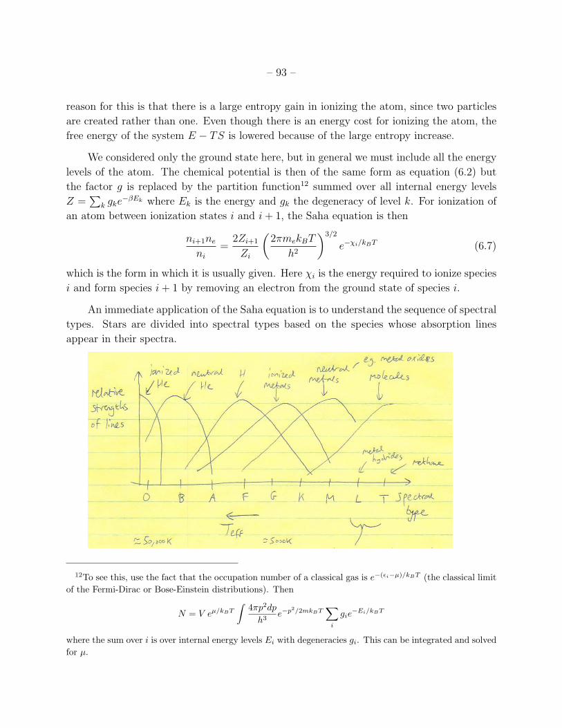
– 93 –

reason for this is that there is a large entropy gain in ionizing the atom, since two particles

are created rather than one. Even though there is an energy cost for ionizing the atom, the

free energy of the system E � TS is lowered because of the large entropy increase.

We considered only the ground state here, but in general we must include all the energy

levels of the atom. The chemical potential is then of the same form as equation (6.2) but

the factor g is replaced by the partition function12 summed over all internal energy levels

Z =P

k gke��Ek where Ek is the energy and gk the degeneracy of level k. For ionization of

an atom between ionization states i and i + 1, the Saha equation is then

ni+1

ne

ni

=2Zi+1

Zi

✓2⇡mekBT

h2

◆3/2

e��i/kBT (6.7)

which is the form in which it is usually given. Here �i is the energy required to ionize species

i and form species i + 1 by removing an electron from the ground state of species i.

An immediate application of the Saha equation is to understand the sequence of spectral

types. Stars are divided into spectral types based on the species whose absorption lines

appear in their spectra.

12To see this, use the fact that the occupation number of a classical gas is e�(✏i�µ)/kBT (the classical limitof the Fermi-Dirac or Bose-Einstein distributions). Then

N = V eµ/kBT

Z4⇡p2dp

h3e�p

2/2mkBT

X

i

gi

e�Ei/kBT

where the sum over i is over internal energy levels Ei

with degeneracies gi

. This can be integrated and solvedfor µ.

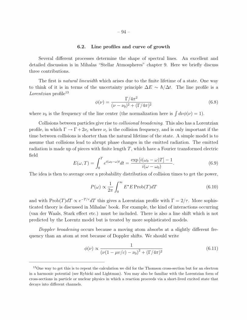
– 94 –

6.2. Line profiles and curve of growth

Several di↵erent processes determine the shape of spectral lines. An excellent and

detailed discussion is in Mihalas “Stellar Atmospheres” chapter 9. Here we briefly discuss

three contributions.

The first is natural linewidth which arises due to the finite lifetime of a state. One way

to think of it is in terms of the uncertainty principle �E ⇠ ~/�t. The line profile is a

Lorentzian profile13

�(⌫) =�/4⇡2

(⌫ � ⌫0

)2 + (�/4⇡)2

(6.8)

where ⌫0

is the frequency of the line center (the normalization here isR

d⌫�(⌫) = 1).

Collisions between particles give rise to collisional broadening. This also has a Lorentzian

profile, in which �! �+2⌫c where ⌫c is the collision frequency, and is only important if the

time between collisions is shorter than the natural lifetime of the state. A simple model is to

assume that collisions lead to abrupt phase changes in the emitted radiation. The emitted

radiation is made up of pieces with finite length T , which have a Fourier transformed electric

field

E(!, T ) =

Z T

0

ei(!0

�!)tdt =exp [i(!

0

� !)T ]� 1

i(! � !0

). (6.9)

The idea is then to average over a probability distribution of collision times to get the power,

P (!) /1

2⇡

Z 1

0

E?E Prob(T )dT (6.10)

and with Prob(T )dT / e�T/⌧dT this gives a Lorentzian profile with � = 2/⌧ . More sophis-

ticated theory is discussed in Mihalas’ book. For example, the kind of interactions occurring

(van der Waals, Stark e↵ect etc.) must be included. There is also a line shift which is not

predicted by the Lorentz model but is treated by more sophisticated models.

Doppler broadening occurs because a moving atom absorbs at a slightly di↵erent fre-

quency than an atom at rest because of Doppler shifts. We should write

�(⌫) /1

(⌫(1� µv/c)� ⌫0

)2 + (�/4⇡)2

(6.11)

13One way to get this is to repeat the calculation we did for the Thomson cross-section but for an electronin a harmonic potential (see Rybicki and Lightman). You may also be familiar with the Lorentzian form ofcross-sections in particle or nuclear physics in which a reaction proceeds via a short-lived excited state thatdecays into di↵erent channels.

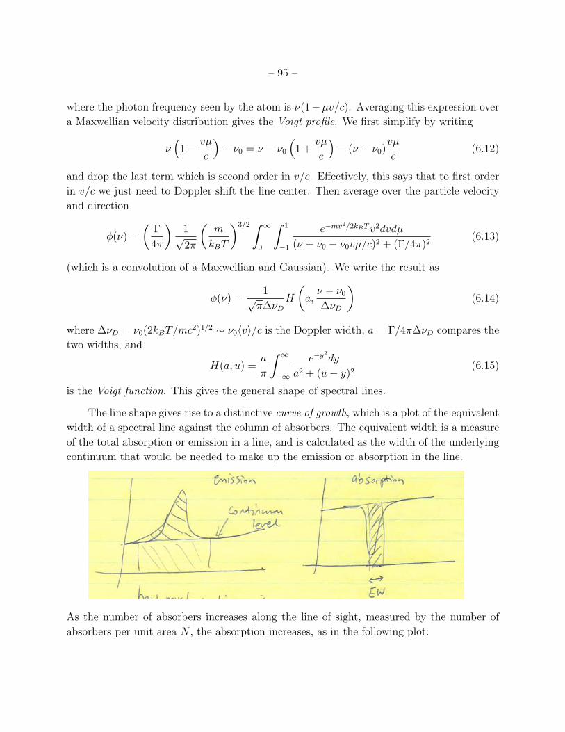
– 95 –

where the photon frequency seen by the atom is ⌫(1�µv/c). Averaging this expression over

a Maxwellian velocity distribution gives the Voigt profile. We first simplify by writing

⌫⇣1�

vµ

c

⌘� ⌫

0

= ⌫ � ⌫0

⇣1 +

vµ

c

⌘� (⌫ � ⌫

0

)vµ

c(6.12)

and drop the last term which is second order in v/c. E↵ectively, this says that to first order

in v/c we just need to Doppler shift the line center. Then average over the particle velocity

and direction

�(⌫) =

✓�

4⇡

◆1p

2⇡

✓m

kBT

◆3/2

Z 1

0

Z1

�1

e�mv2/2kBT v2dvdµ

(⌫ � ⌫0

� ⌫0

vµ/c)2 + (�/4⇡)2

(6.13)

(which is a convolution of a Maxwellian and Gaussian). We write the result as

�(⌫) =1

p

⇡�⌫D

H

✓a,⌫ � ⌫

0

�⌫D

◆(6.14)

where �⌫D = ⌫0

(2kBT/mc2)1/2

⇠ ⌫0

hvi/c is the Doppler width, a = �/4⇡�⌫D compares the

two widths, and

H(a, u) =a

⇡

Z 1

�1

e�y2

dy

a2 + (u� y)2

(6.15)

is the Voigt function. This gives the general shape of spectral lines.

The line shape gives rise to a distinctive curve of growth, which is a plot of the equivalent

width of a spectral line against the column of absorbers. The equivalent width is a measure

of the total absorption or emission in a line, and is calculated as the width of the underlying

continuum that would be needed to make up the emission or absorption in the line.

As the number of absorbers increases along the line of sight, measured by the number of

absorbers per unit area N , the absorption increases, as in the following plot:

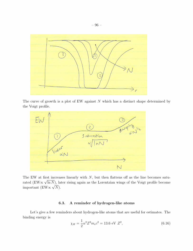
– 96 –

The curve of growth is a plot of EW against N which has a distinct shape determined by

the Voigt profile.

The EW at first increases linearly with N , but then flattens o↵ as the line becomes satu-

rated (EW/p

ln N), later rising again as the Lorentzian wings of the Voigt profile become

important (EW/p

N).

6.3. A reminder of hydrogen-like atoms

Let’s give a few reminders about hydrogen-like atoms that are useful for estimates. The

binding energy is

�H =1

2↵2Z2mec

2 = 13.6 eV Z2, (6.16)

– 97 –

the Bohr radius is

a0

=~

mec

1

Z↵=

0.53 A

Z(6.17)

where

↵ =e2

~c=

1

137(6.18)

is the fine structure constant. The classical electron radius is r0

= ↵2Za0

The spacing

between energy levels is

�Enm = �H

✓1

n2

�

1

m2

◆. (6.19)

Also, now is a good time to remind ourselves of the absorption line series of hydrogen.

The Lyman series corresponds to transitions to n = 1. The Ly limit is 912A, Ly↵ (n = 2

to n = 1) is 1216A, Ly� (n = 3 to n = 1) is 1025A. The Balmer series corresponds to

transitions to n = 2. The Balmer limit is 364.6 nm, H↵ (n = 3 to n = 2) is 656.3 nm, H�

(n = 4 to n = 2) is 486.1 nm.

6.4. Calculation of radiative transitions

In this section, we summarize the main steps in calculating radiative transitions in

atoms. We start with Fermi’s Golden Rule from time-dependent perturbation theory in

non-relativistic quantum mechanics. We consider two eigenstates of the Hamiltonian |ii and

|fi , e.g. H0

|ii = E0

i |ii , and perturb the Hamiltonian H = H0

+ H1

. The transition rate

from state i to f is

Rif =2⇡

~

Z Y

k

d3pk

h3

���hf | H1

|ii���2

�

E0

i � E0

f �

X

k

Ek

!�

~p0

i � ~p0

f �

X

k

~pk

!(6.20)

where the product k is over all final state particles, and the delta-functions enforce energy

and momentum conservation. This is often abbreviated as

Rif =2⇡

~ |Mfi|2 ⇢(E) (6.21)

where Mfi is the matrix element connecting the initial and final states, and ⇢(E) represents

the phase space of the outgoing particles.

To write down H1

for radiative transitions, we need the Hamiltonian of a (non-relativistic)

charged particle in an electromagnetic field,

H =(~p� q ~A/c)2

2m+ q� (6.22)

– 98 –

where ~A and � are the vector and scalar potentials. This Hamiltonian recovers the correct

equations of motion for the charged particle. Expanding the first term, we write

H0

=p2

2m� e� (6.23)

and

H1

=ep · A

mec+

e2

2mec2

A · A (6.24)

(here we have chosen the Coulomb gauge ~r·

~A = 0 so that [A, p] = 0). These terms represent

one and two photon processes. Their ratio is (n�a0

)�1/2 where n� is the photon density, so

that the first term dominates as long as the number of photons per atom is small.

The Hamiltonian for the electromagnetic field is

HEM =1

8⇡

Zd3~r�E2 + B2

�=

1

8⇡

Zd3~r

"✓�

1

c

@A

@t

◆2

+⇣~r⇥

~A⌘

2

#. (6.25)

The photon field is quantized by writing

A =X

~k,�

✓2⇡~c2

!

◆1/2 h

a~k,�~✏⇣~k,�

⌘ei(~k·~r�!t) + a†~k,�

~✏⇣~k,�

⌘e�i(~k·~r�!t)

i(6.26)

where a and a† are annilation and creation operators, satisfying [a~k,�, a†~k,�

] = �~k,~k0��,�0 . Here,

~k is the photon wavevector and � is the spin. This should be familiar to you if you think back

to the harmonic oscillator. Just as in that case, in terms of these operators, the Hamiltonian

is

H =X

~k,�

~!✓

a~k,�a†~k,�

+1

2

◆, (6.27)

and we also have

a~k,�

���n~k,�i =p

n~k,�

���n~k,� � 1i a†~k,�

���n~k,�i =q

n~k,� + 1���n~k,� + 1i . (6.28)

The idea then is that the annhilation and creation operators inside the A factors in the

perturbing Hamiltonian H1

couple the photon states in |ii and |fi . For example, h1 | h�n |

H1

|�mi |0i represents spontaneous emission from state m to n with the emission of a photon.

Now we make a dipole approximation. Substituting our expression for A into H1

, we see

that we have to evaluate

hf | e�i

~k·~r~✏ · p |ii (6.29)

– 99 –

where we drop the prefactor, including the a and a† operators that couple the photon states.

The approximation is to recognize that kr ⇠ (!/c)a0

⇠ Z↵/2 ⌧ 1 and so ei~k·~r⇠ 1. Just as

in the classical dipole approximation, we ignore phase changes across the source. Secondly,

we write

~✏ · hf | p |ii = m~✏ · hf |dr

dt|ii

=im

~ ~✏ · hf | [H, r] |ii

=im

~ (E0

f � E0

i )~✏ · hf | r |ii

= im!~✏ · hf | r |ii . (6.30)

Now we have everything we need to evaluate the rate. We discuss two aspects: first,

the spatial integrals which give rise to selection rules for the transitions, and then estimate

the rate of bound-bound transitions.

6.5. Selection rules from the spatial integral

If the initial and final states are hydrogen-like states, then we need to evaluate

h m | ~✏ · ~r | ki =

Z 1

0

dr r2 R?nf lf

(r) r Rnili(r)

Zd⌦ Y ?

lf mf(✓,�)~✏ · ~er Ylimi

(✓,�). (6.31)

For the angular integral, it is useful to write

~✏ · ~er = ✏x sin ✓ cos�+ ✏y sin ✓ sin�+ ✏z cos�

=

r4⇡

3

✓✏zY1,0 +

�✏x + i✏yp

2Y

1,1 +✏x + i✏yp

2Y

1,�1

◆, (6.32)

which reduces the angular integral to an integral of three Ylm’s,Z

d⌦ Y ?lf ,mf

(✓,�)Yl,mYli,mi(✓,�). (6.33)

Selection rules arise because these integrals are non-vanishing only for particular combi-

nations of initial and final quantum numbers. For example, the azimuthal angular integration

is Zd� e�imf �eim�eimi� = 2⇡�(m�mf + mi) (6.34)

– 100 –

which tells us that mf �mi = m = 1, 0, or �1. Choosing our z axis to lie along the photon

propagation direction, ✏z = 0, we see that m = ±1 only, or

�m = mf �mi = ±1 (6.35)

which is our first selection rule. For example a transition to the ground state has mf = 0 and

therefore must have m = �mi. If mi = 1 then m = �1 and the photon has a polarization

✏x + i✏y (third term in eq. [6.32]), carrying away the angular momentum of the initial state.

Another selection rule that is simple to see is that the parity must change so that the

radial integral is non-vanishingR

d3~r ?f~r i. Since the parity is (�1)l, we conclude that l

must change, and the angular integral gives the constraint

�l = ±1 (6.36)

(e.g. you could check the simple case lf = 0 and use the fact that Y0,0 = 1/

p

4⇡ =constant).

Selection rules for multi-electron atoms are more complex; see Rybicki and Lightman

for details. It is important to note that the selection rules we derived here can be violated

by higher order processes, e.g. magnetic dipole or electric quadrupole transitions.

6.6. Bound-bound transitions

We can now use our results so far to estimate a typical bound-bound transition rate:

Rif ⇠2⇡

~

"e

mec

✓2⇡~c2

!

◆1/2

↵mec

#2

4⇡(~!)2

c3h3

(6.37)

where we use equation (6.26) to estimate the size of A, and p ⇠ ↵mec for hydrogen, and

ignore the overlap integrals; we’re just trying to estimate the magnitude here. The final

factor is the phase space for the outgoing photon. Cancelling factors gives

Rif ⇠2↵2!e2

~c⇠ 2↵3!. (6.38)

Now assume a transition to the hydrogen ground state to get the energy scale, i.e. ~! ⇠(1/2)↵2mec

2. Therefore

Rif ⇠ ↵5

mec2

~ ⇠ ↵4

c

a0

⇠ 1010 s�1. (6.39)

If we had kept the Z scalings, we would find Rif / Z4.

– 101 –

A concrete example is the 2p! 1s transition in hydrogen (Ly↵). The energy is ~!21

=

(3/8)↵2mec2. The radial integral in that case is

Z 1

0

R?10

(r)R21

(r)r3dr =24p

6

✓2

3

◆5

a0

(6.40)

where we use R10

(r) = 2e�r/a0/a

3/2

0

and R21

= re�r/2a0/(p

24a5/2

0

). Averaging over m states

(1/3)P

1

m=�1

R2p!1s(m) gives the final result

R2p!1s = A

21

=

✓2

3

◆8

mec2

~ ↵5 = 0.6⇥ 109 s�1 (6.41)

(the Einstein A coe�cient for the 2p! 1s transition). This is just over an order of magnitude

below our simple estimate.

The Einstein relations allow us to get the cross-section for the reverse process, bound-

bound absorption. Using the results we wrote down relating j⌫ to the Einstein coe�cient

A and ↵⌫ to the Einstein coe�cient B (see the section on synchrotron self-absorption), we

have

�12

=h⌫

4⇡�(⌫)B

12

=g2

g1

�(⌫)c2

8⇡⌫2

A21

=g2

g1

�(⌫)�2

8⇡A

21

(6.42)

where we use the Einstein relations to relate B12

to A21

. Substituting in our expression for

A21

and ⌫21

gives

�12

= f⇡e2

mec�(⌫) (6.43)

where the oscillator strength f = (g2

/g1

)(213/310).

We expect the same scalings for A and � for other transitions, but the prefactor will be

di↵erent, depending on the overlap of the wavefunctions. For example, for transitions to the

ground state, f1n / 1/n3.

6.7. Bound-free transitions: photoelectric e↵ect

Now consider absorption of a photon that excites an electron into the continuum, the

photoelectric e↵ect. Fermi’s Golden Rule for this case is

R =2⇡

~

Zd3~pe

h3

|Mfi|2 �

✓~! � ��

p2

e

2m

◆(6.44)

where we integrate over the phase space of the outgoing electron, and � is the ionization

energy. This can be simplified if we write d3~p = d⌦p2dp = d⌦mpedEe, and integrate over

– 102 –

energy using the delta function, giving

R =2⇡

~

Zd⌦

mpe

h3

|Mfi|2 (6.45)

where pe = 2mp

~! � �. Writing dR/d⌦ = cd�/d⌦, we obtain an expression for the di↵er-

ential cross-sectiond�

d⌦=

2⇡

~c

mpe

h3

|Mfi|2 . (6.46)

The matrix element is the same as previously,

Mfi =e

mec

✓2⇡~c2

!

◆1/2

Zd3~r ?

f ~✏ · ~p ei~k·~r i. (6.47)

As an example, let’s take the initial state to be the hydrogen ground state,

i =1p

⇡

✓1

a0

◆3/2

e�r/a0 (6.48)

and we represent the electron part of the final state as a plane wave (Born approximation)

f / ei~pe·~r/~, (6.49)

giving

hf | ~✏ · pei

~k·~r

|ii = ~✏ · ~pe

hf | ei

~k·~r

|ii , (6.50)

or

|Mfi|2 =

✓e

mec

◆2 2⇡~c2

!

1

⇡a3

0

(~✏ · ~pe)2

����Z

d3~r ei(~k�~pe/~)·~re�r/a0

����2

. (6.51)

The integral is Zd3~r e�i~�·~re�mur =

8⇡µ

(µ2 + �2)2

, (6.52)

which gives (after simplifying)

d�

d⌦= 32a2

0

⇣pec

~!

⌘✓~✏ · ~pe

mec

◆2 1

(1 + a2

0

�2)4

. (6.53)

where

~~� = ~~k � ~pe (6.54)

is the momentum transfer and recall that energy conservation implies Ee = p2

e/2me = ~!��.

A simplification can be made if we assume ~! � � or Ee ⇡ ~!, then

d�

d⌦= 2p

2↵8a2

0

✓Ee

mec2

◆�7/2 sin2 ✓

(1� ve cos ✓/c)4

(6.55)

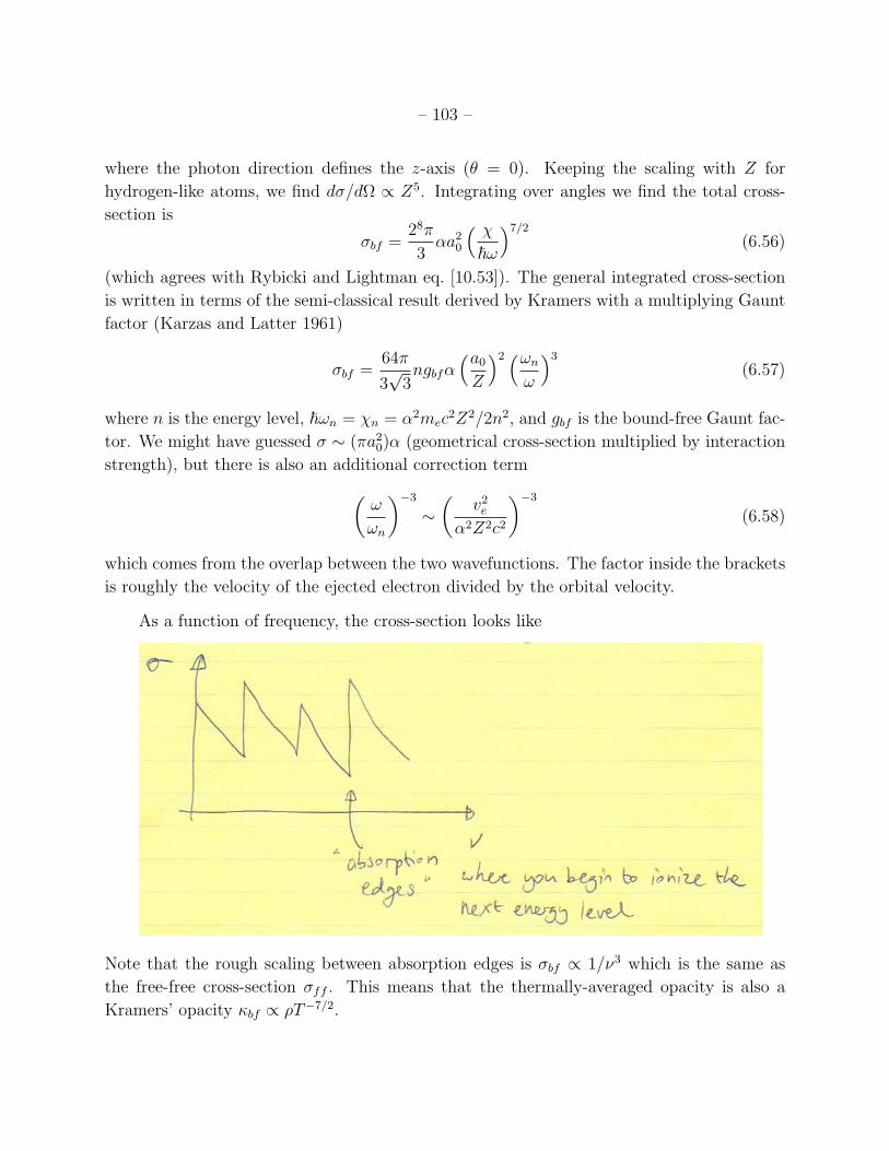
– 103 –

where the photon direction defines the z-axis (✓ = 0). Keeping the scaling with Z for

hydrogen-like atoms, we find d�/d⌦ / Z5. Integrating over angles we find the total cross-

section is

�bf =28⇡

3↵a2

0

⇣ �~!

⌘7/2

(6.56)

(which agrees with Rybicki and Lightman eq. [10.53]). The general integrated cross-section

is written in terms of the semi-classical result derived by Kramers with a multiplying Gaunt

factor (Karzas and Latter 1961)

�bf =64⇡

3p

3ngbf↵

⇣a0

Z

⌘2

⇣!n

!

⌘3

(6.57)

where n is the energy level, ~!n = �n = ↵2mec2Z2/2n2, and gbf is the bound-free Gaunt fac-

tor. We might have guessed � ⇠ (⇡a2

0

)↵ (geometrical cross-section multiplied by interaction

strength), but there is also an additional correction term

✓!

!n

◆�3

⇠

✓v2

e

↵2Z2c2

◆�3

(6.58)

which comes from the overlap between the two wavefunctions. The factor inside the brackets

is roughly the velocity of the ejected electron divided by the orbital velocity.

As a function of frequency, the cross-section looks like

Note that the rough scaling between absorption edges is �bf / 1/⌫3 which is the same as

the free-free cross-section �ff . This means that the thermally-averaged opacity is also a

Kramers’ opacity bf / ⇢T�7/2.

– 104 –

6.8. Bound-free transitions: recombination and the Milne relation

The inverse of the photoelectric e↵ect is recombination. To calculate this we can use

considerations of thermal equilibrium just as we did when deriving the Einstein relations.

We start by deriving the Milne relation,

�bf

�fb

=⇣mcv

h⌫

⌘2 geg+

2gn

. (6.59)

To see this, first write down the number of recombinations per unit time and volume

n+

ne�fbvf(v)dv (6.60)

and the rate of photoionizations per unit volume

nn�bfc

4⇡I⌫

h⌫c

� �1� e�h⌫/kBT

�d⌫ (6.61)

where the factor in square brackets is the photon number density, and we include a correction

for stimulated emission or “stimulated recombination” in this case. In thermal equilibrium,

they must be equal

1 =n

+

ne

nn

�fb

�bf

cvh⌫

4⇡

f(v)

I⌫

dv

d⌫. (6.62)

Now we use results for thermal equilibrium, I⌫ = B⌫ (Planck for photons),

f(v) = 4⇡

✓m

2⇡kBT

◆3/2

v2e�mv2/2kBT (6.63)

(Maxwell-Boltzmann for the electrons), the Saha equation for n+

ne/nn, and since mv2/2 =

h⌫ � �, mvdv = hd⌫ and therefore dv/d⌫ = h/mv. Simplifying, we arrive at the Milne

relation, equation (6.59).

We can apply this relation to get �fb from �bf . The quantity usually given is the

recombination coe�cient (units are cm3 s�1)

hv�fbi =

Zvf(v)�fbdv. (6.64)

Using the expression for �bf and the Milne relation with gn = 2n2, ge = 2, g+

= 1, gives

hv�fbi = 3.262⇥ 10�6 M(n, T ) (6.65)

where

M(n, T ) =e�n/kBT

n3T 3/2

E1

✓�n

kBT

◆(6.66)

– 105 –

(see Cillie 1932) or summed over levels n,

hv�fbi = 5.197⇥ 10�14 �1/2

✓0.4288 +

1

2ln�+ 0.469��1/3

◆cm3 s�1 (6.67)

where � = 13.6 eV/kBT = 1.579⇥ 105 K/T (Seaton 1959).

6.9. Summary of bound-bound and bound-free cross-sections

Let’s summarize our results so far in a form that is useful for making simple estimates

of quantities. First, bound-bound transitions. We have

A21

⇡ Z2↵3! ⇡ Z4↵5

mec2

~ ⇡ 1010Z4 s�1, (6.68)

although we saw that the wavefunction overlap makes this an overestimate, for example

2p! 1s in hydrogen is 6⇥ 108 s�1. The absorption cross-section is

� =g2

g1

�(⌫)A21

�2

8⇡(6.69)

or at the line center,

� ⇡�2

8⇡

A21

�⌫(6.70)

where �⌫ is the width of the line. For example, for Ly↵ (n = 1–2) � = 1216A. If we take

�⌫ ⇡ A21

, then � ⇠ �2/8⇡ = 6⇥ 10�12 cm2.

For bound-free absorption, we have

�bf ⇠↵

n5

⇣a0

Z

⌘2

⇣!n

!

⌘3

⇡

7⇥ 10�18 cm2

n5

⇣!n

!

⌘3

. (6.71)

The recombination coe�cient is hv�fbi ⇠ 10�13 cm3 s�1 and the cross-section is

�fb ⇡ 10�22 cm2

⇣!n

!

⌘✓ ~!n

mv2/2

◆1

n3

. (6.72)

6.10. Application: stellar opacities

We are now (almost) in a position to understand stellar opacities. Both free-free and

bound-free absorption have ⌫ / 1/⌫3 which leads to a Kramers type opacity law, /

⇢T�7/2. Although not obvious why, bound-bound transitions also have a Kramers type

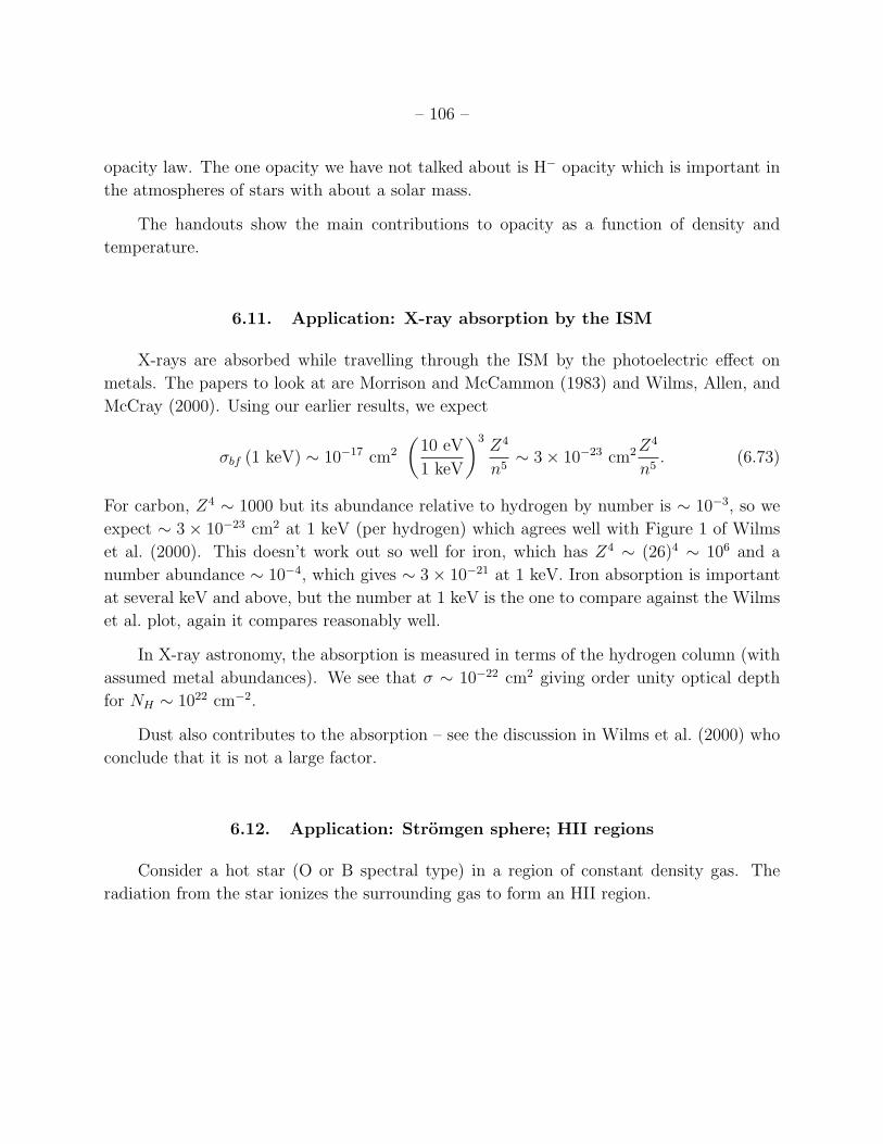
– 106 –

opacity law. The one opacity we have not talked about is H� opacity which is important in

the atmospheres of stars with about a solar mass.

The handouts show the main contributions to opacity as a function of density and

temperature.

6.11. Application: X-ray absorption by the ISM

X-rays are absorbed while travelling through the ISM by the photoelectric e↵ect on

metals. The papers to look at are Morrison and McCammon (1983) and Wilms, Allen, and

McCray (2000). Using our earlier results, we expect

�bf (1 keV) ⇠ 10�17 cm2

✓10 eV

1 keV

◆3

Z4

n5

⇠ 3⇥ 10�23 cm2

Z4

n5

. (6.73)

For carbon, Z4

⇠ 1000 but its abundance relative to hydrogen by number is ⇠ 10�3, so we

expect ⇠ 3⇥ 10�23 cm2 at 1 keV (per hydrogen) which agrees well with Figure 1 of Wilms

et al. (2000). This doesn’t work out so well for iron, which has Z4

⇠ (26)4

⇠ 106 and a

number abundance ⇠ 10�4, which gives ⇠ 3⇥ 10�21 at 1 keV. Iron absorption is important

at several keV and above, but the number at 1 keV is the one to compare against the Wilms

et al. plot, again it compares reasonably well.

In X-ray astronomy, the absorption is measured in terms of the hydrogen column (with

assumed metal abundances). We see that � ⇠ 10�22 cm2 giving order unity optical depth

for NH ⇠ 1022 cm�2.

Dust also contributes to the absorption – see the discussion in Wilms et al. (2000) who

conclude that it is not a large factor.

6.12. Application: Stromgen sphere; HII regions

Consider a hot star (O or B spectral type) in a region of constant density gas. The

radiation from the star ionizes the surrounding gas to form an HII region.

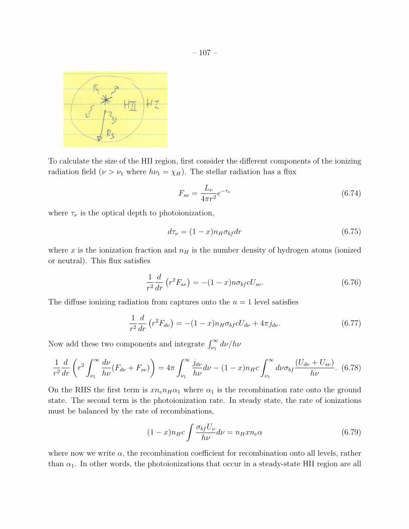
– 107 –

To calculate the size of the HII region, first consider the di↵erent components of the ionizing

radiation field (⌫ > ⌫1

where h⌫1

= �H). The stellar radiation has a flux

Fs⌫ =L⌫

4⇡r2

e�⌧⌫ (6.74)

where ⌧⌫ is the optical depth to photoionization,

d⌧⌫ = (1� x)nH�bfdr (6.75)

where x is the ionization fraction and nH is the number density of hydrogen atoms (ionized

or neutral). This flux satisfies

1

r2

d

dr

�r2Fs⌫

�= �(1� x)n�bfcUs⌫ . (6.76)

The di↵use ionizing radiation from captures onto the n = 1 level satisfies

1

r2

d

dr

�r2Fd⌫

�= �(1� x)nH�bfcUd⌫ + 4⇡jd⌫ . (6.77)

Now add these two components and integrateR1

⌫1

d⌫/h⌫

1

r2

d

dr

✓r2

Z 1

⌫1

d⌫

h⌫(Fd⌫ + Fs⌫)

◆= 4⇡

Z 1

⌫1

jd⌫

h⌫d⌫ � (1� x)nHc

Z 1

⌫1

d⌫�bf(Ud⌫ + Us⌫)

h⌫. (6.78)

On the RHS the first term is xnenH↵1

where ↵1

is the recombination rate onto the ground

state. The second term is the photoionization rate. In steady state, the rate of ionizations

must be balanced by the rate of recombinations,

(1� x)nHc

Z�bfU⌫

h⌫d⌫ = nHxne↵ (6.79)

where now we write ↵, the recombination coe�cient for recombination onto all levels, rather

than ↵1

. In other words, the photoionizations that occur in a steady-state HII region are all

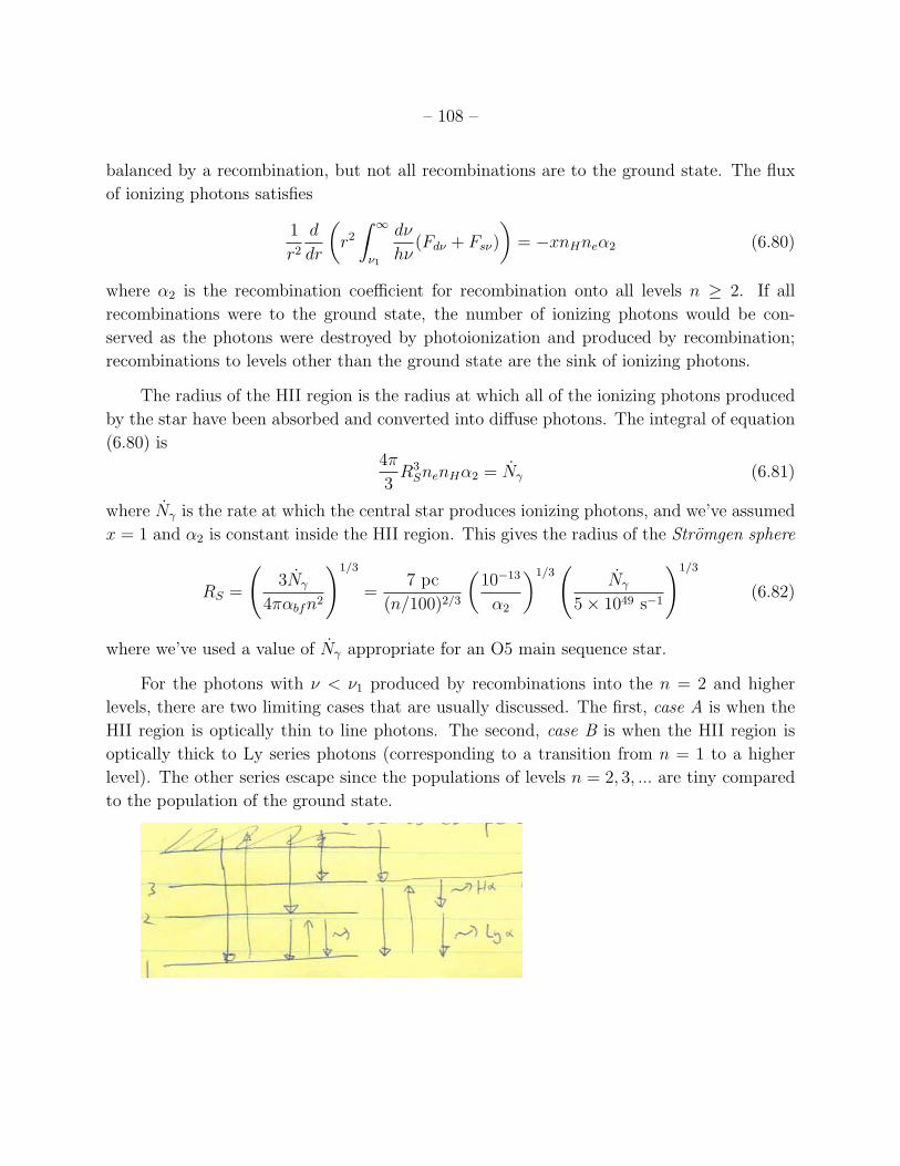
– 108 –

balanced by a recombination, but not all recombinations are to the ground state. The flux

of ionizing photons satisfies

1

r2

d

dr

✓r2

Z 1

⌫1

d⌫

h⌫(Fd⌫ + Fs⌫)

◆= �xnHne↵2

(6.80)

where ↵2

is the recombination coe�cient for recombination onto all levels n � 2. If all

recombinations were to the ground state, the number of ionizing photons would be con-

served as the photons were destroyed by photoionization and produced by recombination;

recombinations to levels other than the ground state are the sink of ionizing photons.

The radius of the HII region is the radius at which all of the ionizing photons produced

by the star have been absorbed and converted into di↵use photons. The integral of equation

(6.80) is4⇡

3R3

SnenH↵2

= N� (6.81)

where N� is the rate at which the central star produces ionizing photons, and we’ve assumed

x = 1 and ↵2

is constant inside the HII region. This gives the radius of the Stromgen sphere

RS =

3N�

4⇡↵bfn2

!1/3

=7 pc

(n/100)2/3

✓10�13

↵2

◆1/3

N�

5⇥ 1049 s�1

!1/3

(6.82)

where we’ve used a value of N� appropriate for an O5 main sequence star.

For the photons with ⌫ < ⌫1

produced by recombinations into the n = 2 and higher

levels, there are two limiting cases that are usually discussed. The first, case A is when the

HII region is optically thin to line photons. The second, case B is when the HII region is

optically thick to Ly series photons (corresponding to a transition from n = 1 to a higher

level). The other series escape since the populations of levels n = 2, 3, ... are tiny compared

to the population of the ground state.

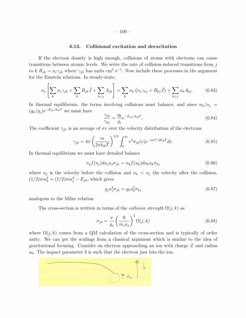
– 109 –

6.13. Collisional excitation and deexcitation

If the electron density is high enough, collisions of atoms with electrons can cause

transitions between atomic levels. We write the rate of collision-induced transitions from j

to k Rjk = ne�jk where �jk has units cm3 s�1. Now include these processes in the argument

for the Einstein relations. In steady-state,

nj

"X

k

ne�jk +X

k

BjkJ +X

k<j

Ajk

#=X

k

nk

�ne�kj + BkjJ

�+X

k>j

nkAkj. (6.83)

In thermal equilibrium, the terms involving collisions must balance, and since nk/nj =

(gk/gj)e�Ejk/kBT we must have�jk

�kj

=gk

gj

e�Ejk/kBT . (6.84)

The coe�cient �jk is an average of �v over the velocity distribution of the electrons

�jk = 4⇡

✓m

2⇡kBT

◆3/2

Z 1

0

v3�jk(v)e�mv2/2kBT dv. (6.85)

In thermal equilibrium we must have detailed balance

njf(uj)dujuj�jk = nkf(uk)dukuk�kj (6.86)

where uj is the velocity before the collision and uk < uj the velocity after the collision,

(1/2)mu2

k = (1/2)mu2

j � Ejk, which gives

gju2

j�jk = gku2

k�kj (6.87)

analogous to the Milne relation.

The cross-section is written in terms of the collision strength ⌦(j, k) as

�jk =⇡

gj

✓~

meuj

◆2

⌦(j, k) (6.88)

where ⌦(j, k) comes from a QM calculation of the cross-section and is typically of order

unity. We can get the scalings from a classical argument which is similar to the idea of

gravitational focusing. Consider an electron approaching an ion with charge Z and radius

a0

. The impact parameter b is such that the electron just hits the ion.

– 110 –

Conservation of angular momentum and energy conservation gives

bvi = avf v2

f = v2

i +2Ze2

ma0

. (6.89)

The cross-section is

� = ⇡b2 = ⇡a2

0

✓1 +

2Ze2

ma0

v2

i

◆. (6.90)

The second term in the brackets dominates: using a0

= (~/mec)(1/Z↵), we find it is

2Z2↵2c2/v2

i ⇠ 10Z2(T/104 K)�1, where we write vi ⇡ (3kBT/me)1/2 = 6.7 km s�1T 1/2.

The cross-section is then

� ⇡ ⇡a2

0

✓2Ze2

ma0

v2

i

◆= 2⇡

✓~

mevi

◆2

. (6.91)

Averaging over the electron velocity distribution usingR1

0

udue�l2u2

= 1/2l2 gives the

deexcitation rate as

�kj =h2⌦(j, k)

gk(2⇡me)3/2(kBT )1/2

= 8.63⇥ 10�6 cm3 s�1

⌦(j, k)

gkT 1/2

. (6.92)

The excitation rate coe�cient is given by14 gj�jk = gk�kje�Ejk/kBT .

6.14. Line diagnostics of temperature and density

Consider a two-level system. In equilibrium,

n1

ne�12

+ n1

B12

J = n2

ne�21

+ n2

A21

+ n2

B21

J (6.93)

which givesn

2

n1

=ne�12

+ B12

J

ne�21

+ B21

J + A21

=ne�12

/A21

+ B12

J/A21

1 + JB21

/A21

+ ne�21

/A21

. (6.94)

Now using the Einstein relations B21

/A21

= c2/2h⌫3, B12

/A21

= (g2

/g1

)(c2/2h⌫3) and �12

=

�21

(g2

/g1

)e�E12

/kBT , we get

n2

n1

=(g

2

/g1

)e�E12

/kBT�ne�12

/A21

+ eE12

/kBT c2J/2h⌫3

�

1 + c2J/2h⌫3 + ne�21

/A21

. (6.95)

14Using the relation in eq. [6.84] that we derived using arguments about thermal equilibrium. You can alsodirectly average the excitation cross-section over the electron velocity distribution, but be careful - if you dothat you must take into account the fact that a minimum energy (1/2)mv2 = E

jk

is required to excite thetransition. Including this as a lower limit on the range of velocities considered gives the factor of e�Ejk/kBT

that we deduced from thermal equlibrium.

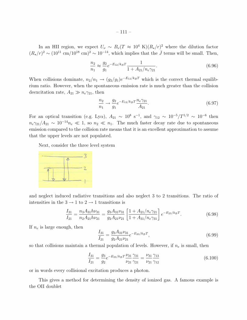
– 111 –

In an HII region, we expect U⌫ ⇠ B⌫(T ⇡ 104 K)(R?/r)2 where the dilution factor

(R?/r)2

⇠ (1011 cm/1018 cm)2

⇠ 10�14, which implies that the J terms will be small. Then,

n2

n1

⇡

g2

g1

e�E12

/kBT 1

1 + A21

/ne�21

. (6.96)

When collisions dominate, n2

/n1

! (g2

/g1

)e�E12

/kBT which is the correct thermal equilib-

rium ratio. However, when the spontaneous emission rate is much greater than the collision

deexcitation rate, A21

� ne�21

, then

n2

n1

!

g2

g1

e�E12

/kBT ne�21

A21

. (6.97)

For an optical transition (e.g. Ly↵), A21

⇠ 108 s�1, and �12

⇠ 10�5/T 1/2

⇠ 10�6 then

ne�21

/A21

⇠ 10�14ne ⌧ 1, so n2

⌧ n1

. The much faster decay rate due to spontaneous

emission compared to the collision rate means that it is an excellent approximation to assume

that the upper levels are not populated.

Next, consider the three level system

and neglect induced radiative transitions and also neglect 3 to 2 transitions. The ratio of

intensities in the 3! 1 to 2! 1 transitions is

I31

I21

=n

3

A31

h⌫31

n2

A21

h⌫21

=g3

A31

⌫31

g2

A21

⌫21

1 + A

21

/ne�21

1 + A31

/ne�31

�e�E

23

/kBT . (6.98)

If ne is large enough, thenI31

I21

=g3

A31

⌫31

g2

A21

⌫21

e�E23

/kBT , (6.99)

so that collisions maintain a thermal population of levels. However, if ne is small, then

I31

I21

=g3

g2

e�E23

/kBT ⌫31

⌫21

�31

�21

=⌫

31

⌫21

�13

�12

(6.100)

or in words every collisional excitation produces a photon.

This gives a method for determining the density of ionized gas. A famous example is

the OII doublet

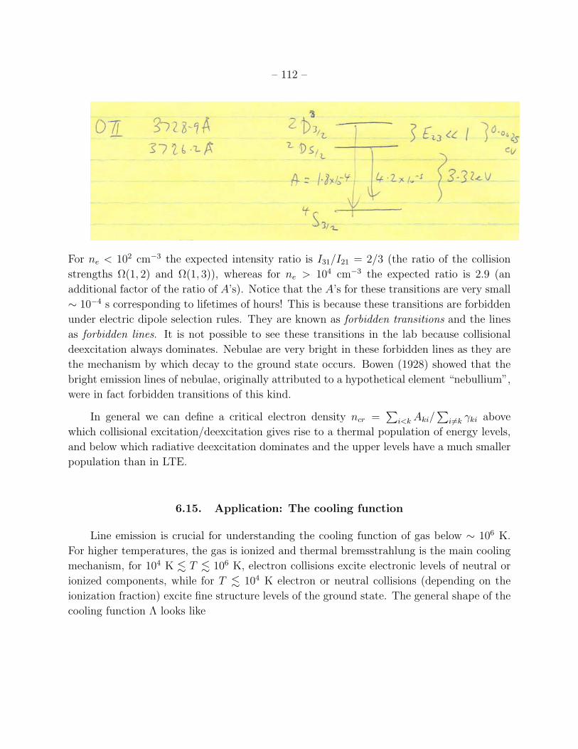
– 112 –

For ne < 102 cm�3 the expected intensity ratio is I31

/I21

= 2/3 (the ratio of the collision

strengths ⌦(1, 2) and ⌦(1, 3)), whereas for ne > 104 cm�3 the expected ratio is 2.9 (an

additional factor of the ratio of A’s). Notice that the A’s for these transitions are very small

⇠ 10�4 s corresponding to lifetimes of hours! This is because these transitions are forbidden

under electric dipole selection rules. They are known as forbidden transitions and the lines

as forbidden lines. It is not possible to see these transitions in the lab because collisional

deexcitation always dominates. Nebulae are very bright in these forbidden lines as they are

the mechanism by which decay to the ground state occurs. Bowen (1928) showed that the

bright emission lines of nebulae, originally attributed to a hypothetical element “nebullium”,

were in fact forbidden transitions of this kind.

In general we can define a critical electron density ncr =P

i<k Aki/P

i6=k �ki above

which collisional excitation/deexcitation gives rise to a thermal population of energy levels,

and below which radiative deexcitation dominates and the upper levels have a much smaller

population than in LTE.

6.15. Application: The cooling function

Line emission is crucial for understanding the cooling function of gas below ⇠ 106 K.

For higher temperatures, the gas is ionized and thermal bremsstrahlung is the main cooling

mechanism, for 104 K . T . 106 K, electron collisions excite electronic levels of neutral or

ionized components, while for T . 104 K electron or neutral collisions (depending on the

ionization fraction) excite fine structure levels of the ground state. The general shape of the

cooling function ⇤ looks like

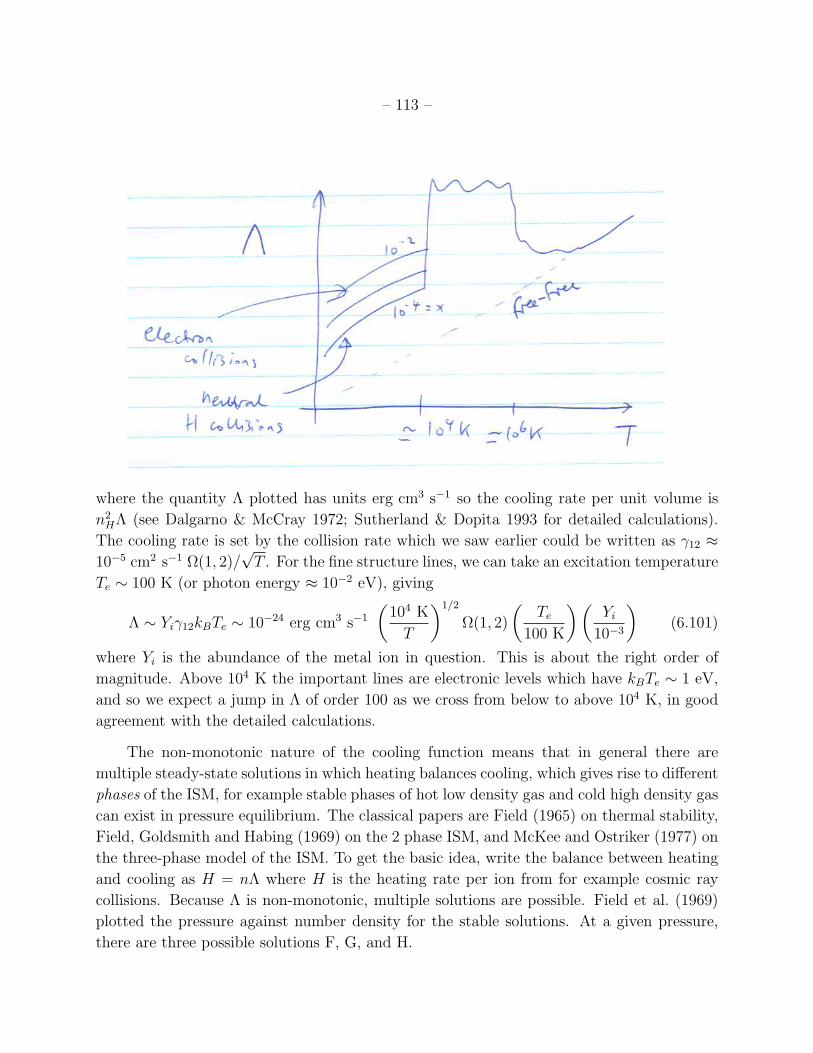
– 113 –

where the quantity ⇤ plotted has units erg cm3 s�1 so the cooling rate per unit volume is

n2

H⇤ (see Dalgarno & McCray 1972; Sutherland & Dopita 1993 for detailed calculations).

The cooling rate is set by the collision rate which we saw earlier could be written as �12

⇡

10�5 cm2 s�1 ⌦(1, 2)/p

T . For the fine structure lines, we can take an excitation temperature

Te ⇠ 100 K (or photon energy ⇡ 10�2 eV), giving

⇤ ⇠ Yi�12

kBTe ⇠ 10�24 erg cm3 s�1

✓104 K

T

◆1/2

⌦(1, 2)

✓Te

100 K

◆✓Yi

10�3

◆(6.101)

where Yi is the abundance of the metal ion in question. This is about the right order of

magnitude. Above 104 K the important lines are electronic levels which have kBTe ⇠ 1 eV,

and so we expect a jump in ⇤ of order 100 as we cross from below to above 104 K, in good

agreement with the detailed calculations.

The non-monotonic nature of the cooling function means that in general there are

multiple steady-state solutions in which heating balances cooling, which gives rise to di↵erent

phases of the ISM, for example stable phases of hot low density gas and cold high density gas

can exist in pressure equilibrium. The classical papers are Field (1965) on thermal stability,

Field, Goldsmith and Habing (1969) on the 2 phase ISM, and McKee and Ostriker (1977) on

the three-phase model of the ISM. To get the basic idea, write the balance between heating

and cooling as H = n⇤ where H is the heating rate per ion from for example cosmic ray

collisions. Because ⇤ is non-monotonic, multiple solutions are possible. Field et al. (1969)

plotted the pressure against number density for the stable solutions. At a given pressure,

there are three possible solutions F, G, and H.

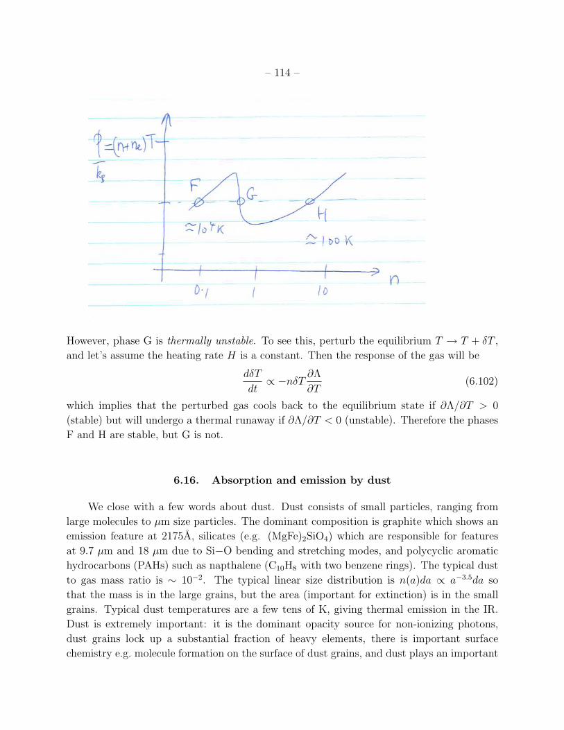
– 114 –

However, phase G is thermally unstable. To see this, perturb the equilibrium T ! T + �T ,

and let’s assume the heating rate H is a constant. Then the response of the gas will be

d�T

dt/ �n�T

@⇤

@T(6.102)

which implies that the perturbed gas cools back to the equilibrium state if @⇤/@T > 0

(stable) but will undergo a thermal runaway if @⇤/@T < 0 (unstable). Therefore the phases

F and H are stable, but G is not.

6.16. Absorption and emission by dust

We close with a few words about dust. Dust consists of small particles, ranging from

large molecules to µm size particles. The dominant composition is graphite which shows an

emission feature at 2175A, silicates (e.g. (MgFe)2

SiO4

) which are responsible for features

at 9.7 µm and 18 µm due to Si�O bending and stretching modes, and polycyclic aromatic

hydrocarbons (PAHs) such as napthalene (C10

H8

with two benzene rings). The typical dust

to gas mass ratio is ⇠ 10�2. The typical linear size distribution is n(a)da / a�3.5da so

that the mass is in the large grains, but the area (important for extinction) is in the small

grains. Typical dust temperatures are a few tens of K, giving thermal emission in the IR.

Dust is extremely important: it is the dominant opacity source for non-ionizing photons,

dust grains lock up a substantial fraction of heavy elements, there is important surface

chemistry e.g. molecule formation on the surface of dust grains, and dust plays an important

– 115 –

role in energy balance. Here, we focus on how to understand the typical dust absorption

cross-section, and the dust temperature.

The dust optical depth is generally written as

⌧ = L

Z a+

a�

n(a)da�d(a)Qext

(�, a)L (6.103)

where L is the path length, �d = ⇡a2 is the geometric cross-section for a sphere, and “ext”

refers to extinction which can be due to absorption or scattering (when the dust lies along

the line of sight to an object scattering removes photons from the beam), so that

Qext

(�, a) = Qabs

(�, a) + Qsca

(�, a). (6.104)

In astronomy, the extinction in magnitudes at a given wavelength A� = �2.5 log10

(e⌧�) =

1.086⌧�. Commonly dust extinction will be measured in AV the visual extinction. This is

related to the hydrogen column,

NH ⇡ 5.9⇥ 1021 cm�2 mag�1 EB�V (6.105)

where EB�V = AB �AV is the di↵erence between the B and V band extinctions. The slope

of the extinction curve near V band is RV = AV /EB�V with RV commonly taken to be 3.1

(can be as large as 5 for lines of sight into dense clouds).

For calculations of the optical properties of grains, cross-sections and dust temperatures

see Draine and Lee (1984). To calculate the absorption and scattering cross-sections from

first principles requires understanding the optical properties of the grains, in other words the

refractive index n or dielectric constant ✏ = n2. The dielectric constant is complex in general,

and the solutions for scattering and absorption by small particles are known as Mie theory.

For spherical particles, and in the long-wavelength limit x = 2⇡a/� ⌧ 1, the cross-sections

are

Qsca

=8

3x4

����✏� 1

✏+ 2

����2

/

1

�4

(6.106)

(Rayleigh scattering) and

Qabs

= 4x Im

✓✏� 1

✏+ 2

◆/

1

�. (6.107)

For short wavelength photons x� 1, Qsca

! 1 and Qabs

! 1. We’ve written the wavelength

scalings here for constant ✏. In fact, ✏ depends on frequency in general which changes the

scaling. The extinction cross-section is usually written

Qext

= Q0

✓�

0

�

◆�

(6.108)

– 116 –

with � = 1–2. For graphite and silicates the long wavelength emission has � ⇡ 2.

We can get the cross-sections in equations (6.106) and (6.107) from a straightforward

calculation along the lines of the classical derivation of the Thomson cross-section. A di-

electric sphere in a uniform electric field has an induced dipole moment ~p = ↵~E, where

the polarizability ↵ = 4⇡✏0

a3(✏ � 1/✏ + 2) (SI units). Plugging this into Larmors formula

P = (1/2)(!4p2/6⇡✏0

c3) and dividing by the incoming flux c✏0

E2/2 gives the scattering

cross-section in equation (6.106). The absorption cross-section is obtained by calculating

the work done ~J ·

~E, where ~J is the polarization current

@ ~P

@t=

i!~p

4⇡a3/3. (6.109)

The power dissipated is⇣~J ·

~E⌘✓4

3⇡a3

◆= i!~p ·

~E = i!↵E2 (6.110)

or taking a time average!

2Im(↵)E2. (6.111)

Again, dividing by the incoming flux in the wave gives the cross-section, which agrees with

equation (6.107).

The equilibrium dust temperature is given by balancing heating with cooling. The

heating rate is

4⇡a2

Z⇡J�Qabs

(�, a)d�. (6.112)

For short wavelength UV and optical photons which are responsible for most of the heating,

Qabs

⇠ 1 in which case we can write the heating rate as 4⇡2a2JUV where JUV is the mean

intensity of the photons with wavelengths shorter than typical dust sizes. The cooling or the

dust emissivity we can get from Kircho↵’s law, giving

4⇡a2

Z⇡B�(Td)Qabs

(�, a)d� (6.113)

where Td is the dust temperature. The dust temperature is therefore given by

JUV =

ZB�(Td)Qabs

(�, a)d�. (6.114)

For typical dust temperatures Td ⇡ 20 K, we need the absorption cross-section near � =

0.29 cm/T ⇡ 200 µm. Writing Qabs

= Q0

(�0

/�)� = (2⇡a/�)(�0

/�)��1 gives

JUV =

Z2⇡a

�

✓�

0

�

◆��1 2h⌫3

c2

1

eh⌫/kBT� 1

d⌫

d�d� =

4⇡a���1

0

h

c2+�

✓kBTd

h

◆4+� Z

x3+� dx

ex� 1

(6.115)

– 117 –

or Td / (JUV /a)1/(4+�). For 0.1 µm size grains, the temperatures are ⇡ 20K.

An interesting situation arises for small grains (Purcell 1976). A 100A grain at 20 K has

a thermal content of ⇠ 1 eV. Partly this is due to the (T/⇥D)3 suppression of the specific

heat at low temperatures, where the Debye temperature ⇥D is typically hundreds of K.

The temperature of these grains is time-dependent since absorption of a photon significantly

changes the thermal energy, followed by rapid cooling. The observed emission of small grains

can therefore be at significantly higher temperature, e.g. 50K (see Purcell 1976).

Summary and Further Reading

Here are the main ideas and results that we covered in this part of the course:

• Saha equation. Ionization of hydrogen at T ⇡ 104 K. Application to stellar spectral

types.

• Line profiles. Natural line width ⇤. Collisional broadening. Doppler broadening

�⌫/⌫ ⇡ hvi/c. Voigt function. Definition of equivalent width. Curve of growth.

• Hydrogen-like atoms. � = (1/2)Z2↵2mec2, a

0

= (~/mec)↵�1Z�1, Enm = �(n�2

�m�2).

• Calculation of radiative transitions. Fermi’s Golden Rule. Hamiltonian for a charged

particle in an electromagnetic field. Origin of selection rules in the spatial integrals.

• Bound-bound transitions. Einstein A coe�cients: A ⇠ (mc2/~)↵5. Ly↵ has A =

0.6 ⇥ 109 s�1. Bound-bound absorption cross-section: �12

= f(⇡e2/mec)�(⌫) or ⇡

(�2/8⇡)(A21

/�⌫), where �⌫ is the linewidth.

• Bound-free (photoionization) cross-section

�bf = ↵⇡a2

0

Z2

⇣!n

!

⌘3 64

3p

3ngbf

Absorption edges. bf / ⇢T�3.5. Milne relations. Recombination coe�cient h�fbvi ⇠

10�14 cm3 s�1. Application to HII regions. The Stromgen sphere. Case A and case B.

Application to X-ray absorption by the ISM.

• Collisional excitation and dexcitation. Cross-section �jk = (⇡/gj)(~/mev)2⌦(j, k).

Averaging over a Maxwell-Boltzmann distribution of velocities gives the deexcitation

rate coe�cient

�kj =8.6⇥ 10�6 ⌦(j, k)

gkT 1/2

cm3 s�1.

– 118 –

The excitation rate coe�cient is then �jk = (gk/gj)e�Ejk/kBT�kj. The critical density

ne,c = A21

/�21

. Application: the use of forbidden line ratios as a probe of density. The

importance of line emission in the cooling function.

• Dust. Sizes, composition, dust to gas ratio, temperatures, importance. The basic

idea of scattering and absorption by small particles. For � � a, � / 1/�4 (Rayleigh

scattering, constant ✏). Generally, Qext

/ ��� with � = 1–2.

Reading

• RL chapter 10. The calculation of radiative transitions is covered at the end of most

introductory quantum books, e.g. the books by Gasiorowicz and Townsend. Shu also

has a lot of detail on this.

• Radial integrals of hydrogen-like wavefunctions: Gordon (1929) Ann Phys 2, 1031.

• Osterbrock ”Astrophysical Gaseous Nebulae” is the classic book to look up cross-

sections and transition rates etc. A classic but somewhat dated book on ISM physics

is by Spitzer. Recombination coe�cients: Cillie 1932, MNRAS, 92, 820. Seaton 1959,

MNRAS, 119, 81.

• X-ray absorption by the ISM: Wilms, Allen, & McCray (2000), Morrison & McCammon

(1983).

• Cooling function: Dalgarno & McCray (1972), Sutherland & Dopita (1993). Thermal

stability and multi-phase interstellar medium: Field (1965), Field, Goldsmith & Habing

(1969), McKee & Ostriker (1977).

• Dust: Mathis (1990 ARAA), Draine & Lee (1984 ApJ).