PHYS 371: Electrons Laboratory Laboratory Manualfrantz/phys371/manual371.pdf · PHYS 371: Electrons Laboratory Laboratory Manual ... 4 The ratio Charge-to-Mass of the electron 21

PHYS 371: Electrons LaboratoryLaboratory Manual

Julie Roche and Carl Brune

September 30, 2010

Contents

1 Laboratory general directions 3

1.1 General conduct in the laboratory . . . . . . . . . . . . . . . . . . . . . . . . 3

1.2 Guidelines to prepare yourself to perform an experiment: Run plan . . . . . 4

1.3 Reporting experimental work . . . . . . . . . . . . . . . . . . . . . . . . . . 4

2 Statistics and treatment of experimental data 10

2.1 Physical concepts . . . . . . . . . . . . . . . . . . . . . . . . . . . . . . . . . 10

2.2 Reading and homework assignments . . . . . . . . . . . . . . . . . . . . . . . 10

2.3 Tutorial . . . . . . . . . . . . . . . . . . . . . . . . . . . . . . . . . . . . . . 12

3 The Hall Effect 15

3.1 Physical concept . . . . . . . . . . . . . . . . . . . . . . . . . . . . . . . . . 15

3.2 Experimental setup and procedure suggestion . . . . . . . . . . . . . . . . . 18

3.3 Lab objectives . . . . . . . . . . . . . . . . . . . . . . . . . . . . . . . . . . . 18

3.4 Preliminary questions . . . . . . . . . . . . . . . . . . . . . . . . . . . . . . . 19

4 The ratio Charge-to-Mass of the electron 21


4.2 Experimental setup . . . . . . . . . . . . . . . . . . . . . . . . . . . . . . . . 22

4.3 Lab objectives . . . . . . . . . . . . . . . . . . . . . . . . . . . . . . . . . . . 22

4.4 Determining the radius of curvature . . . . . . . . . . . . . . . . . . . . . . . 22


5 Electron diffraction 25


5.2 Experimental setup . . . . . . . . . . . . . . . . . . . . . . . . . . . . . . . . 28

5.3 Lab objectives . . . . . . . . . . . . . . . . . . . . . . . . . . . . . . . . . . . 28


1

6 The Millikan’s oil drop experiment 336.1 Physical concept . . . . . . . . . . . . . . . . . . . . . . . . . . . . . . . . . 336.2 Experimental setup . . . . . . . . . . . . . . . . . . . . . . . . . . . . . . . . 356.3 Lab objectives . . . . . . . . . . . . . . . . . . . . . . . . . . . . . . . . . . . 376.4 Preliminary questions . . . . . . . . . . . . . . . . . . . . . . . . . . . . . . . 37

7 The Franck-Hertz Experiment 397.1 Physical concept . . . . . . . . . . . . . . . . . . . . . . . . . . . . . . . . . 397.2 Experimental setup and procedure suggestion . . . . . . . . . . . . . . . . . 437.3 Lab objectives . . . . . . . . . . . . . . . . . . . . . . . . . . . . . . . . . . . 447.4 Preliminary questions . . . . . . . . . . . . . . . . . . . . . . . . . . . . . . . 44

2

1 Laboratory general directions

1.1 General conduct in the laboratory

These directions are to be considered a guide to your laboratory work rather than a recipeto be followed blindly.

- Come prepared: Before the lab session, prepare by reading this manual and doinganalysis in between sessions. Bring the necessary supplies and submit your reportpromptly. Also, if you ask the instructor for help between sessions bring your notesas it is much easier to talk about your data then to talk in general terms of theexperiment.

- Be safe: Be careful with the equipment as you take data in order to protect yourselfand the equipment. Especially, you will be using equipment which poses some hazardssuch as high-voltage power supplies. Listen to safety instructions and heed them. Alsoif a piece of equipment is not working even after you have followed all instructions, becareful what you fiddle with! Some fiddling is good, but if you are planning anythingmajor (like taking a piece of equipment apart), it is EXTREMELY IMPORTANT toask the instructor first. Also it is good lab practice not to eat or drink in the lab: youmight damage the equipment and/or eat or drink something you don’t intend to!

- Understand the purpose of the experiment: Think of the purpose of the experiment sothat you know why you are doing each step. A scientist or engineer knows what is to bemeasured before the experiments begins (i.e., Are you measuring a constant, verifyinga law?). In addition, professional scientists and engineers are paid for their work andconsequently do not do things without a good reason. Do not depend upon yourpartner to do your thinking for you. Plan your laboratory activities for the greatesteconomy of time and effort. Often a few minutes of preliminary manipulation of theapparatus will save an hour of repeating the experiment due to taking worthless datahurriedly. Laboratory work is a joint venture. Carry your share of the responsibility.Don’t leave the lab without making sure you understand your data and have recordedsufficient information to allow the data to be analyzed later. If you are unsure of aprocedure, ask a laboratory assistant.

- Record data completely and honestly: Record what you observe, not what you hope itshould be (or what someone else says it is). Keep a good laboratory book and recordyour data and the steps you take! Write down data in a neat and organized way.Don’t think it is a trivial task. Feel free to ask your instructor for advices on how toaccomplish this. The goal is to be able to read and understand what you did afteryou leave the laboratory. Do not be tempted to falsify data (in this course or later inyour career). Sometimes there may be pressure to do this. Those who succumb to thepressure are usually found out and the ramifications are very serious. These incidentsare damaging to society and the credibility of the scientific professions. The careersof the scientists responsible are typically severely damaged by these incidents.

3

- Cross-check your data: There are a variety of honest mistakes that an experimentalistcan make in recording or in analyzing data. One possible mistake is to assume that anobserved signal is due to the sample when it is actually due to the instrumentation.Another mistake is to reach the wrong conclusion in analyzing data. It may be difficultto avoid this pitfall. Perhaps the best advice is to urge caution, especially if you havesome doubts. Publishing a mistake and then publishing a retraction is embarrassingand may damage one’s career. For this lab, if the final result has intolerably largeerrors (more than 25% unless otherwise indicated), repeat the experiment after findingout what is wrong. If you find that the error cannon be reduced, you are expected toexplain why this is the case. You are not being graded on the “correctness” of yourdata.

- Investigate: Look out for refinements in technique and equipment which indicate acarefully and well-performed experiment with the least error possible. For example,in an experiment with pulleys and a force table, one refinement is to make sure thatall pulleys are the same size. Feel free to innovate and improve the apparatus andprocedure if you can. Record these changes in your report. Also, when doing anexperiment, it is important for the experimentalist not to accept the data as correctwithout adequately questioning it. Always be curious.

1.2 Guidelines to prepare yourself to perform an experiment:Run plan

The following questions are typically answered before hand by someone well prepared toperform an experiment. In this class, you are expected to answer these questions duringthe first session dedicated to an experiment. After discussing with your lab partner, writedown your plan and turn in your answers to the instructor before leaving class.

- What are the goals of this experiment?

- What is the method used to achieve these goals? Write down a list of steps detailingthe sequence of your work.

- What quantities will I measure? You may want to prepare tables that you will fillduring the data taking.

1.3 Reporting experimental work

In addition to planning and thinking about the experiment to be done and optimizingthe equipment and technique as indicated, there are several other important aspects ofexperimental work. These are: (1) organizing data and results into graphs and tables toaid in interpreting the experiment, (2) error analysis, and (3) writing a report to help incommunicating the results to other scientists. The error analysis treatment will be explainedin its own chapter later in this manual. A very good guide for how to write a report andorganize your data was produced by the Pomona College of California and can be found at:

4

http://www.physics.pomona.edu/sixideas/labs/LRM/LR08.pdf

or on the web site of the class. The grading system for the lab reports is given in Table 1.Various aspects of report writing are discussed below.

1.3.1 Sections in the scientific report

The following sections should be included in the technical report. It is good to look attextbooks to see how equations, graphs, figures, tables and statements are handled.

- Abstract: The abstract should be a very short and concise description of what is inthe report. Its purpose is to help others who may be looking up the literature on aparticular subject. They should be able to read the abstract in a matter of secondsand know if this report will be of any help to them. Only when they decide thatit will be of use will they read through the actual report. This cuts down on thetime spent searching the literature. The abstract should contain a short statementof: (1) the purpose of the experiment, (2) the methods used, (3) the results, and (4)the conclusions reached as to verification of theory and the causes of any significanterrors. For this class, the abstract should not be longer than five complete sentences.

- Introduction: The introduction section is meant to provide the reader with the an-swers to two very important questions: ”What is the question that your experimentis supposed to answer?” and ”Why is answering this question interesting (and/or im-portant)?”. This section often begins with a brief summary of current knowledge. Itcontinues with a statement of a problem that this knowledge raises, a brief descriptionof the experiment presented in your paper, and how it addresses the question asked.Detailed descriptions are not appropriate in this section. The point is to provide aconcise picture of your purposes and a broad survey of your approach.

- Theory: This section should contain a complete exposition of the theory, includingthe physical phenomena and equations behind the experiment as found in varioustextbooks of physics. It should include derivations (or references derivations) of theformulas used in the experiment from from underlying principles. Figures may beincluded. Be sure to include proper citations to this lab manual or other sources.Remember that all variables and symbols must be defined and used consistently; donot use the same variable or symbol for more than one quantity! Equations shouldbe numbered sequentially and reference where appropriate. Use your textbooks forexamples of how to properly include equations grammatically into your text. For thepurposes of this course, I would encourage you not to put an excessive amount of effortinto derivations and figures for the theory section. I would prefer to see most of yourefforts directed towards the exposition of your own work in the other sections.

- Experimental apparatus and procedure: This section should include a description of theequipment and how it was used. A schematic line drawing of the equipment and/orany critical components should be included. Finally, this section should include acomplete description of the data that were taken as well as the rational for takingthem. The data should be organized into tables if appropriate. The quantity and

5

units must be given, with sufficient and reasonable significant figures. This sectionshould also include estimates of any expected systematic errors and random errors.

- Analysis: This section should include at least three sub-sections: (1) Method of anal-ysis, (2) Presentation of the results, and (3) Discussion of the results. The variouscalculated values should be included here in clear tabular form, as appropriate. Graphsand tables should have titles and should help you to see trends and relations. Use yourand other textbooks as models for your tables and graphs. Table columns and theaxes of graphs must give the quantities and their units. Proper handling of significantfigures is important. The slope and intercept of a graph often have important physicalsignificance and should be explained. The discussion should include an interpretationof the graphs and tables. The level of agreement between the experiment and theoryshould also be discussed. It may also be appropriate to discuss problems with theexperiment or possible improvements here.

- Conclusions: The conclusions should contain a summary of the outcome(s) of theexperiment: the experimental results (with errors) and their agreement (or not) withtheory. The conclusions reached must be explained and justified. Remarks aboutpossible further research or other issues can also be included. The conclusion is im-portant and should show considerable thought about the experiment. Note that inthe working world, many people will only read the introduction and conclusion of yourreport. There is often some redundancy between between the discussion subsection ofthe analysis and the conclusions section. I suggest that you limit this redundancy byonly including the most important conclusions and issues in this section.

- Bibliography: The bibliography must contain a list of all works cited in the report. Itis important that sufficient information be provided so that somebody else can findthe reference. Your format should be consistent; a good reference for formatting is:

http://authors.aps.org/STYLE/ms.html#footnotes

which gives the format used by the Physical Review family of journals (the mostwidely-used physics journals in the United States). An example of an item in abibliography is:F.V. Hunt, Electro-acoustics (John Wiley, New York, 1954), p. 124.

An outline of your report could for example look like this:

ABSTRACT

1. INTRODUCTION

A. Motivation (that is what are the goals of your experiment)

B. Summary of the experiment you performed

2. THEORETICAL BACKGROUND

6

3. EXPERIMENTAL PROCEDURE

A. Description of apparatus including the operating ranges of the devices

B. Description of experimental procedure

C. Description in plain English of the observed phenomena

D. Description of sources of errors separating the systematic and random error

4. ANALYSIS1

A. Method of analysis including precision estimation

B. Presentation of results

C. Discussion of results

D. (optional) Suggestions for future improvements

5. CONCLUSIONS

A. Summary of results

B. Pertinence of results to the questions raised in the introduction

1.3.2 General comments on style

Your report is expected be of high quality. The report must be original, well organized,complete and precise. It must be correct with respect to grammar and spelling. After writingthe report, read over it, watch for lack of precision and for ambiguity. Each sentence shouldpresent a clear message. Here are a few tips:

- With regard to precision, you should qualify what is written so that there is no questionas to what was done or concluded. For example, instead of saying, ”The temperaturedependence of the surface tension of water was measured”, you should be more preciseand complete and say, ”The temperature dependence of the surface tension of waterwas measured in the range 20 C to 60 C”. Avoid using only adjectives as they aresubject to interpretation and always try to make quantitative statements.

- The data and results should be well organized in tables and the graphs should be neatwith legends on each axis explaining the quantity plotted and its units, a title and acaption. Figure 1 is an example of a graph with a proper caption and legend. Tables,figures and equations should be numbered for easy access (for example see Table 2,Figure 4, Equation 39). All tables and figures must be referenced and explained inthe report. Tables and figures may be interspersed throughout the text, or includedat the very end of the report.

1If your experiment had multiple goals or parts you might want to create multiple analysis sections.

7

Figure 1: Example of the proper way to present a figure in a report. Observe the legendon each axis, the use of different symbols to disentangle the data and the numbering of thisfigure. Note how the caption points spells out what the figure is about.

- Avoid using the first person, ”I” or ”we” in writing. Instead of writing ”We weighedthe frogs and put them in a glass jar”, write ”The frogs were weighed and put in aglass jar”. Be consistent in the use of the tense throughout the paper - do not switchbetween past and present. Using past tense is standard. Be sure that pronouns referto antecedents. For example, in the statement ”Sometimes cecropia caterpillars are inthe cherry trees but they are hard to find,” does “they are hard to find” refer to thecaterpillars or the trees?

- Use metric system of measurements. Abbreviation of units are used without a fol-lowing period (for example 2 mm or 6 g). Number should be written as numeralswhen they are greater than ten or when they are associated with measurements. Forexample: 2 mm or 6 g but two explanations or six factors. Spell out numbers thatbegin sentences.

Additional References

D. Preston and E. Dietz, The Art of Experimental Physics (Wiley, New York, 1991).Physical Review Style and Notation Guide (http://authors.aps.org/STYLE/). This is agood source of grammar, punctuation, abbreviation, etc... information.The undergraduate lab manual for the Ohio University 250 series.

8

Student: Lab: (0: not acceptable, → 3: correct)

your pts weight total

Structure of the report (A) 1.Summarize the entire paper in abstract 0 1 2 3State the problem and summarize procedure in introduction 0 1 2 3Introduce all relevant variables in the theory section 0 1 2 3Show considerable after-though about the experiment in the conclusion 0 1 2 3Presentation (B) 1.Quote results with proper precision, significant figures, and units 0 1 2 3Display relevant equations properly 0 1 2 3Give appropriate legends and headings to tables, graphs and sketches 0 1 2 3Use logical transition words and sentences to tie together the report 0 1 2 3

Procedure (C) 1.Provide a sketch and a description of the experimental setup 0 1 2 3Report the precision and operating range of the apparatus 0 1 2 3Completely discuss all precautions taken to make a good measurement 0 1 2 3Describe all measurements as well as the rational to take them 0 1 2 3Describe in plain English the phenomena you are observing∗ 0 1 2 3

Analysis (D) 3.Report the data on proper tabular form 0 1 2 3Show sample calculation(s) 0 1 2 3Recognize and quantify the main sources of uncertainty∗∗ 0 1 2 3Show details of your precision determination 0 1 2 3Present well-chosen graphs of the data that includes error bars 0 1 2 3

Completeness (E) 2.Fulfill all of the experimental objectives of the lab 0 1 2 3Fulfill all of the theoretical objectives of the lab 0 1 2 3Thoroughness of data taking 0 1 2 3

Final grade: A+B+C+D+E /100∗This should be at least 5 sentences long. ∗∗List separately random and systematic errors.

Comments:

Table 1: The grading system for the PHYS 371 the lab reports. Note that the sum of pointsis actually 102, so there are two “bonus points” (in some sense).

9

2 Statistics and treatment of experimental data

2.1 Physical concepts

There is no such thing as a perfect experiment. Each measurement contains some degree ofuncertainty due to the limits of instruments and the people using them. In physics, theseof uncertainties are called errors (think of the error as the difference between the measuredvalue and the true underlying value). We will consider two distinct error concepts: accuracyand precision. Precision refers to how close together a group of measurements actually areto each other. It is often called random error or statistical error. The accuracy of themeasurement refers to how close the measured value is to the true or accepted value, afteraveraging over many measurements so that the error due to precision is negligible. Theaccuracy is often called the systematic error. Precision has nothing to do with the trueor accepted value of a measurement, so it is quite possible to be very precise and totallyinaccurate. In many cases, when precision is high and accuracy is low, the fault can lie withthe instrument.2

2.2 Reading and homework assignments

The following book is the required reading for this class3.P.R. Bevington and D.K. Robinson, ”Data reduction and error analysis for the physicalsciences,” ISBN 0-07-247227-8.

- For the second class: Read Chap 1, work out exercises 1.3 and 1.5.

- For the third class: Read Chap 2, work out exercises: 2.8, 2.13.

- For the fourth class: Read Chap 3, work out exercises: 3.5, 3.6.

- For the fifth class: Read Chap 4, work out exercises: 4.5 and 4.12 (skip t-distributionquestion).

- For the sixth class: Read Chap 6, work out exercise given in class.

2.2.1 Important formulas

Straight average: This method applies when one performs a set of N measurements ofa given quantity xi with equal precision ∆xi = ∆x for each measurement. For this sample,the mean value is x, the standard deviation of the sample is σx and should be equal to ∆x,and the precision on the mean is ∆x:

x =1

N

∑xi σx =

√1

N − 1

∑(xi − x)2 ∆x =

σx√N. (1)

2This section is based on a document of the Fordham Preparatory School.3Another excellent reference is: .R. Taylor, “An introduction to error analysis, The study of uncertainties

in physical measurements,” ISBN 0-935702-75

10

Weighted average: This method applies when one performs a set of N measurementsof a given quantity xi with different precisions ∆xi for each measurement. For this sample,the mean value is x, and the precision on the mean is ∆x:

x =

∑(xi/∆x

2i )∑

(1/∆x2i )

∆x =1√∑

(1/∆x2i ). (2)

χ2 minimization: A numerical comparison between the observed distribution of mea-surements xi with precisions ∆xi and a function y can be defined via χ2:

χ2 =∑ (xi − y)2

∆x2i

(3)

The number of degrees of freedom ν is defined to be the number of data points minus thenumber of free parameters in the function y. The “best fit” is determined by minimizing χ2.The minimum value of χ2 should be approximately equal to ν. The reduced χ2 is definedto be χ2

ν = χ2/ν.

Linear fit: Suppose a set of measurements of xi, yi and ∆yi, from which one to extract alinear function of the form y(x) = ax+ b. One way to extract the parameters a and b is tominimize the χ2 between the data and the function. The solution for the least-squares fitof a straight line is:

a =EB − CADB − A2

b =DC − EADB − A2

(4)

(∆a)2 =B

DB − A2(∆b)2 =

D

DB − A2(5)

where

A =∑ xi

(∆yi)2B =

∑ 1

(∆yi)2(6)

C =∑ yi

(∆yi)2D =

∑ x2i

(∆yi)2(7)

E =∑ xiyi

(∆yi)2F =

∑ y2i

(∆yi)2(not used). (8)

Note that in many real life experiments, the measured quantities are xi±∆xi and yi±∆yi.How to deal with errors on both x and y is a non-trivial and sometimes controversial issue.For the purpose of this class and in this case, if on supposes yi = f(xi), one should translate∆xi into a ∆yi error by replacing ∆yi with√

(∆yi)2 + (∂f

∂xi∆xi)2. (9)

11

2.3 Tutorial

This exercise is extracted from “An introduction to error analysis: The study of uncertain-ties in physical measurements,” 2nd edition, J.R. Taylor, University Science Book.

Systematic errors sometime arise when an experimenter unwittingly measures the wrongquantity. Here is an example.

Gravity can be measured using a pendulum made of a steel ball suspended by a lightstring. Gravity g can then be extracted using the following formula:

g = 4π2l/T 2 (10)

where l is the length of the pendulum and T is its period. A student tries to measure gusing this method. He records six different lengths of the pendulum l and the correspondingperiods T . He estimates that his precision on the measurement of the length is 0.1 cm andon the periods is 0.0005 s. His data are presented in table 2.

Length l (cm) 51.2 59.7 68.2 75.0 79.7 88.3Period T (s) 1.4485 1.5655 1.669 2.098 1.8045 1.896

Table 2: Measurements of the length and the period of the pendulum

1. For each pair (li, Ti), he calculates gi. He then calculates the mean gm of those values,their standard deviation σm and their standard deviation of mean ∆gm, assumingall his errors are random. What is his answer for gm ± ∆gm? He now compares hisanswer with the accepted value g = 979.6 cm/s2 and he is horrified to realize that hisdiscrepancy is nearly 10 times larger than his uncertainty. Confirm this sad conclusion.

2. Studying his results, the student notices that the values gi he extracted from his resultsseem to increase as the period T increases which might be the sign of systematic bias.He decides to check if his observation is correct.

First he computes the precision of each of his measurements gi, i.e.,

(∆g)2 =

(∂g

∂l∆l

)2

+

(∂g

∂T∆T

)2

(11)

Using his set of gi and ∆gi values, he recomputes gw±∆gw using the weighted averagemethod. How does gm and gw compare? Why are they different? Which methodshould be used to compute the average value of g? Explain your answer.

Then he plots gi ±∆gi as a function of T 2 and draws the line corresponding to gw onhis plots. Reproduce his plot. Finally, he computes the χ2 of gw compared to his dataand concludes that indeed there is bias in his data. What is the χ2, the reduced χ2

and the probability of his data being independent of T 2? Why would you say, like thestudent did, that there is a bias in his data?

12

3. Having checked his calculations and found them to be correct, the student concludesthat he must have overlooked some systematic errors. He is sure there was no problemwith the measurement of the period T and that the problem must be in his measure-ment of l. So he asks himself: How large would a systematic error in the length lhave to be so that his result would be the accepted value 979.6 cm/s2? Show that theanswer is approximately 1.5%.

4. In order to make a maximum usage of his data, the student decides to extract thebest value of his systematic error on the length l by performing a linear fit of his data.First he rewrites Equation 10 to take into account his supposed systematic error l0such that he measured l when he should have measured l − l0:

T 2g + 4π2l0 = 4π2l (12)

Then he plots 4π2l versus T 2 such that the slope of straight line is g and the offset is4π2l0. Reproduce this plot, don’t forget the error bars. Using the linear fit method,extract gl ±∆gl, as well as l0 ±∆l0. How does the reduced χ2 of this fit compared tothe case where l0 was ignored? What does it mean?

5. This result would mean that the student’s length measurement suffered a systematicerror of about a centimeter – a conclusion he first rejects as absurd. As he staresat the pendulum, he realizes that 1 cm is about the radius of the steel ball andthat the lengths he recorded were the lengths of the string. Because the correctlength of the pendulum is the distance from the pivot to the center of the ball, hismeasurements were indeed systematically off by the radius of the ball (see Figure2). He, therefore, uses a caliper to find the ball’s diameter, which turns out to be2.00±0.01 cm. Make the necessary corrections to his data and compute his finalresult for gf with its uncertainties. Don’t forget to take into account the precision onthe ball radius. Justify your choice to use the straight average method or the weightedaverage method. What about the χ2 of the corrected values of g?

l−l0l

Figure 2: A pendulum consists of a metal ball suspended by a string. The effective length ofthe pendulum (l) is the length of the string (l-l0) plus the radius of the ball.

13

14

3 The Hall Effect

The Hall Effect was discovered by E. Hall in 1879 while working on his doctoral thesis. Hall’sexperiments consisted of exposing thin gold leaf (and, later, using various other materials) ona glass plate and tapping off the gold leaf at points down its length. The effect is a potentialdifference (Hall voltage) on opposite sides of a thin sheet of conducting or semiconductingmaterial (the Hall element) through which an electric current is flowing. This was createdby a magnetic field applied perpendicular to the Hall element. The ratio of the voltagecreated to the amount of current is known as the Hall Resistance and is a characteristic ofthe material in the element. In 1880, Hall’s experimentation was published as a doctoralthesis in the American Journal of Science and in the Philosophical Magazine. One veryimportant feature of the Hall Effect is that it differentiates between positive charges movingin one direction and negative charges moving in the opposite. The Hall Effect offered thefirst real proof that electric currents in metals are carried by moving electrons, not byprotons. The Hall Effect also showed that in some substances (especially semiconductors),it is more appropriate to think of the current as positive ”holes” moving rather than negativeelectrons.

3.1 Physical concept

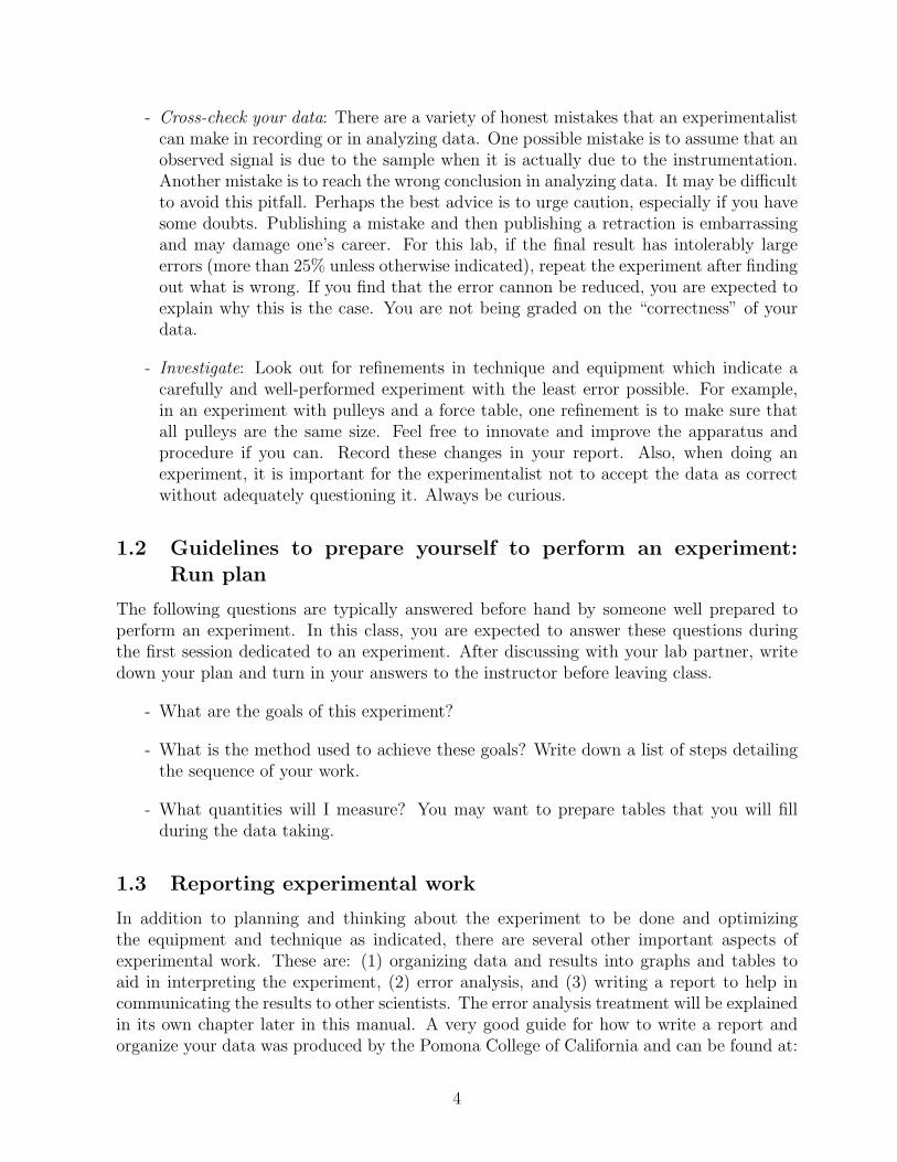
The Hall Effect comes about due to the nature of the current flow in the conductor. Currentconsists of many small charge-carrying ”particles” (typically electrons) which experience aforce (called the Lorentz Force) when in the presence of a magnetic field (see figure 3) .When a perpendicular magnetic field is absent, there is no Lorentz Force and the chargefollows an approximate ’line of sight’ path. When a perpendicular magnetic field is present,the path is curved perpendicular to the magnetic field due to the Lorentz Force. The resultis an asymmetric distribution of charge density across the Hall element perpendicular tothe ’line of sight’ path the electrons would take in the absence of the magnetic field. As aresult, an electric potential is generated between the two ends.

For a metal or for a n- or p-type semiconductor4 at normal temperature, electric con-duction is due to a single carrier type with charge q and mobility µ. If a magnetic field ~B isapplied along the axis z as on Figure 4, then the carrier of charge q experiences a LorentzForce :

~F = q( ~E + ~v × ~B) (13)

If the definition of carrier mobility is expanded to include magnetic forces, the drift velocityis given by :

~v = ±µ( ~E + ~v × ~B) (14)

where the plus and minus sign is used for holes and the minus sign is used for electrons.For this configuration of fields, the drift velocity components are related by

vx = ±µ(Ex + vyBz) vy = ±µ(Ey − vzBx) vz = ±µEz (15)

4You may want to refresh your knowledge on semiconductors

15

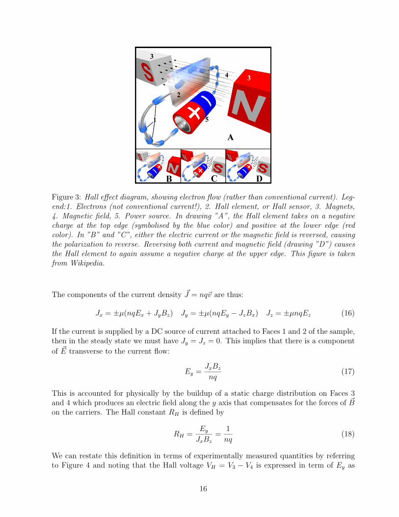
Figure 3: Hall effect diagram, showing electron flow (rather than conventional current). Leg-end:1. Electrons (not conventional current!), 2. Hall element, or Hall sensor, 3. Magnets,4. Magnetic field, 5. Power source. In drawing ”A”, the Hall element takes on a negativecharge at the top edge (symbolised by the blue color) and positive at the lower edge (redcolor). In ”B” and ”C”, either the electric current or the magnetic field is reversed, causingthe polarization to reverse. Reversing both current and magnetic field (drawing ”D”) causesthe Hall element to again assume a negative charge at the upper edge. This figure is takenfrom Wikipedia.

The components of the current density ~J = nq~v are thus:

Jx = ±µ(nqEx + JyBz) Jy = ±µ(nqEy − JzBx) Jz = ±µnqEz (16)

If the current is supplied by a DC source of current attached to Faces 1 and 2 of the sample,then in the steady state we must have Jy = Jz = 0. This implies that there is a component

of ~E transverse to the current flow:

Ey =JxBz

nq(17)

This is accounted for physically by the buildup of a static charge distribution on Faces 3and 4 which produces an electric field along the y axis that compensates for the forces of ~Bon the carriers. The Hall constant RH is defined by

RH =EyJxBz

=1

nq(18)

We can restate this definition in terms of experimentally measured quantities by referringto Figure 4 and noting that the Hall voltage VH = V3 − V4 is expressed in term of Ey as

16

Vt

l

xy

z

2

34

1w

B

Figure 4: A Hall sample is a conducting sample through which a current I is flowing. Forthe Hall voltage to appear, the sample needs to be in region where a magnetic field B exists.The current I flows from face 1 to face 2. The resulting Hall Voltage appears between face3 and 4, that is perpendicularly to both the current I and the magnetic field B. This figureis taken from Preston.

VH = wEy, and that Jx = I/wt. Thus, the experimental Hall Coefficient normalized by thethickness t of the sample is expressed in terms of measurable quantities as

RH

t=

VHIBz

(m2/C) (19)

Note that the carrier density in this case can be calculated directly from a measurementof RH , and that the sign of RH can be used to determine the sign of the charge carriers.This, of course, means that careful analysis of the signs of I, Bz, as well as VH needs to beperformed.

3.1.1 Thermo-magnetic effects

Because of several thermo-magnetic effects, the measured voltage V34 = V3 − V4 may notbe the ”true” Hall voltage VH (see figure 4). Reference5 gives a concise description of theNernst Effect, the Righi-Leduc Effect, and the Ettingshausen Effect, along with suggestionsfor reducing their respective contributions to measured voltages. The Ettingshausen Effectcannot be separated from the Hall Effect in the present experiment but will be small insamples with good bulk thermal conduction. The Nernst and Righi-Leduc effects, alongwith any residual IR drop, can be compensated by averaging V34 over both directions ofcurrent and field. Thus the Hall voltage corresponding to a current I and a field B shouldbe taken as an average of four separate measurements:

VH =1

4(V34(I, B)− V34(I,−B)− V34(−I, B) + V34(−I,−B)) (20)

3.1.2 To go further

- What is the quantum Hall Effect?

5O. Lindberg, Proc IRE 40, 1414 (1952): A brief discussion of the Hall effect in semiconductors and thethermo-magnetic effects that complicates measurements of the Hall voltages

17

3.2 Experimental setup and procedure suggestion

The Hall apparatus used in this lab is a product of the Leybold Cie. A copy of the operatingmanual for this device is available on the class web site, it describes the apparatus as wellas suggest a procedure for the experiment. Figure 5 is extracted from this manual anddescribes roughly how the apparatus should be setup. The Silver foil you will be workingwith is 50 µm thick. Setting up the experiment has revealed it self as a little tricky, hereare some typical results to consider:

- When the electromagnet is setup correctly, one measures a magnetic field of ∼ 0.7 Tfor a current of ∼ 5 A,

- When the whole apparatus is correctly setup, the Hall voltage for a Silver foil sunkinto a ∼ 0.7 T magnetic field and traversed by a current of 15 A is 16 µV.

Figure 5: Typical arrangement for the Hall apparatus.

3.3 Lab objectives

- Verify the proportionality of the Hall voltage with the magnetic flux density and thecurrent through the sample.

- Determine the Hal constant RH and the charge carrier concentration of Silver andcompare to literature. Do not forget to quote your results with their error bars. Theliterature value of RH for Silver is 8.9 10−11 m3/C, the concentration of charge carrierfor Silver is 6.6 1028 m−3.

- Determine the polarity of the charge carriers in Silver

18

3.4 Preliminary questions

The following questions should help you prepare for this lab:

- Describe at least 4 industrial applications of the Hall Effect.

- What are magnetic hysteresis and magnetic saturation for an electromagnet?

- Because of several thermo-magnetic effects, the voltage V34 measured on a semi-conductor, may not be the ”true” Hall voltage VH (see section 3.1.1). For exampleV34 = VH + Vbias. What are the name of the effects creating Vbias? For your datataking, how will you deal with this issue?

- Suppose you measure RH/t for a fixed magnetic field B0 and three different currentsthrough the Hall probe. Suppose you know B0 and I to 1% relative precision andeach V34 to 1%. What is the final relative precision on RH/t ? How much of this israndom, and how much of this is systematic?

- The number density of free electrons in gold is 5.90 1028 electrons per cubic meter. Ifa metal strip of gold 2 cm wide carries a current of 10 A, how thin would it need tobe to produce a Hall Voltage of at least one 1 mV. What would the drift velocity ofthe electrons be in this case? (Assume a perpendicular field of 5000 Gauss)

References

The discussion of the Hall Effect is taken up from ”Wikipedia, The Free Encyclopedia” aswell as from “The art of experimental physics”, D. Preston, ISBN 0-471-84748-8.

19

20

4 The ratio Charge-to-Mass of the electron

J.J. Thomson first measured the charge-to-mass ratio of the fundamental particle of chargein a cathode ray tube in 1897. A cathode ray tube basically consists of two metallic platesin a tube which has been evacuated and filled with a very small amount of backgroundgas. One plate is heated and “particles” boil off of the cathode and accelerate toward theother plate which hold a positive potential. The gas in between the two plates inelasticallyscatters the electrons, emitting light which shows the path of the particles. The charge-to-mass ratio of the particle can be measured by observing their motion in an appliedmagnetic field. Thomson repeated his measurement of e/m many time with different metalsand also different gases. Having reached the same value of e/m every time, he concludedthat a fundamental particle having a negative charge e and a mass 2000 times less thanthe lightest atoms existed in all atoms. Thomson named these particle “corpuscles,” butwe now know them electrons. In this lab, you will essentially repeat Thomson’s experimentand measure e/m for electrons.


The mass-to-charge ratio is a physical quantity that is widely used in the electrodynamicsof charged particles, e.g., in electron optics and ion optics. It appears in the scientificfields of lithography, electron microscopy, cathode ray tubes, accelerator physics, nuclearphysics, auger spectroscopy, cosmology and mass spectrometry. The importance of themass-to-charge ratio is that according to classical electrodynamics two particles with thesame mass-to-charge ratio move in the same path in a vacuum when subjected to the sameelectric and magnetic fields.The magnetic force Fm acting on a charged particle of charge q moving with velocity v in amagnetic field B is given by the equation

Fm = q~v × ~B (21)

In the case where the initial velocity is perpendicular to the magnetic field, the equationcan be written in scalar form as:

Fm = evB (22)

Since the electrons are moving in a circle, they must be experiencing a centripetal force ofmagnitude

Fc = mv2/r (23)

where m is the mass of the electron, v is its velocity, and r is the radius of the circularmotion. Since the only force acting on the electrons is that caused by the magnetic field,Fm = Fc. So Equations 22 and 23 can be combined to give

e

m=

v

Br(24)

Therefore, in order to determine e/m, it is only necessary to know the velocity of theelectrons, the magnetic field and the radius of the circle described by the electrons. Sup-pose electrons are accelerated from a quasi-null speed through the accelerating potential

21

V , gaining kinetic energy equal to their charge times the accelerating potential. Therefore,eV = 1/2mv2. The velocity of the electron is:

v =

√2eV

m(25)

Suppose also that the magnetic field in which the electron beam travels is produced nearthe axis of a pair of Helmholtz coils. The magnetic field B is, therefore:

B =Nµ0I

(5/4)3/2a(26)

where µ0 is the magnetic permeability6, I is the current through the Helmholtz coil, a isthe radius of the Helmholtz coils, and N is the number of turns on each Helmholtz coil. Inthis case, the final formula for e/m is:

e/m =2V (5/4)3a2

(Nµ0Ir)2(27)

4.1.1 To go further

Mass spectroscopy is a widely used technique. How does it work ? How does it relate tothe e/m experiment?

4.2 Experimental setup

A stream of electrons is accelerated by having them fall through a measured potential differ-ence. This stream is projected into a uniform magnetic field, perpendicular to the velocityvector of the electrons that cause the electrons to bend into a circular path. An electronbeam tube with Helmholtz coils will be provided. The circular path of the electrons willbe used to measure the the ratio e/m. A copy of the operating manual for the CENCOapparatus you will be using is available on the class website.

4.3 Lab objectives

To measure the ratio of e/m for electrons and to compare it to the accepted world data.

4.4 Determining the radius of curvature

This lab requires that one determine the radius of the the electron trajectory from measure-ments of the trajectory in Cartesian coordinates. How does one do this? One approach is tochoose three points from the trajectory, and use those points to determine the radius, sincethree points (in a 2-dimensional plane) uniquely determine a circle. I suggest utilizing twopoints from near the respective ends of the trajectory and one from near the middle (why?).

6µ0 = 4π10−7Tm/A

22

The following formulas are from the Wolfram MathWorld website (given below). Assumingan arbitrary triangle with sides of length a, b, and c, one can define the the semiperimeters:

s ≡ 1

2(a+ b+ c). (28)

The area A of the triangle is then given by Heron’s Formula:

A =√s(s− a)(s− b)(s− c) (29)

and the circumradius R is given by

R =abc

4A. (30)

The circumradius is the radius of the circumscribed circle – in other words the radius ofthe circle which intersects the three vertices of the triangle. It is thus also the radius of ourelectron trajectory. Note that the lengths a, b, and c can be easily determined from theCartesian coordinates using the Pythagorean Theorem.


The following questions should also help you to prepare for this lab:

- What are Helmholtz coils and what are they used for? Draw a diagram showing themagnetic field profile along the axis crossing the center of the coils for 3 differentsetups : 1) the coils are separated by a distance larger than their radius, 2) the coilsare separated by a distance equal to their radius, 3) the coils are separated by adistance smaller than their radius.

- Suppose you perform 4 measurements of e/m by choosing one magnetic field andvarying the accelerating voltage. Suppose you know the current through the coil, theaccelerating voltage and the radius of the electron trajectory to 1%. What is the finalrelative precision of e/m? Which part of the error is systematic precision and whichpart is random?

- Assuming the Helmholtz coils have a radius of 10 cm, 130 turns and are powered with2A. The accelerating voltage is typically 100 V. How does the magnetic field theycreate compare to Earth magnetic field?

- Classical mechanics was used to derive the equations used in this experiment. Evaluatethe value of β = v/c used in determining the charge-to-mass ratio of the electron forthe setup described above. Based on these values of β, can relativistic corrections beneglected?

- Draw a diagram with the following features: a region of space containing a magneticfield pointing into the page, the path an electron would follow if injected into thisspace with a certain velocity initially pointing upward, and the path a proton wouldfollow if injected in this same space with the same velocity.

23

References

- The SSS Theorem, from the Wolfram MathWorld website:http://mathworld.wolfram.com/SSSTheorem.html

24

5 Electron diffraction

A primary tenet of quantum mechanics is the wave-like properties of matter. In 1924,graduate student Louis de Broglie suggested in his dissertation that since light has bothparticle-like and wave-like properties, perhaps all matter might also have wave-like prop-erties. He postulated that the wavelength of object was given by l = h/p, where p = mvis the momentum. This was quite a revolutionary idea, since there was no evidence at thetime that matter behaved like waves. De Broglie received a Nobel prize in 1929 for hisdiscovery of the wave nature of electron. In 1927, however, C. Davisson and L. Germer,and G. Thomson independently discovered experimental proof of the wave-like propertiesof matter -particularly electrons. Davisson and Thomson won the Nobel Prize in 1937 fortheir experimental discovery of the diffraction of electrons by crystal. Not only was thisdiscovery important for the foundation of quantum mechanics, but electron diffraction is anextremely important tool used to study new material.


De Broglie’s Law states that:

λ =h

p(31)

where λ is the electron wave length, h is the Planck’s Constant and p is the electron mo-mentum. For an electron accelerated through a potential V , the momentum p is given bythe following relation:

p =√

2meV (32)

where m is the mass of the electron and e its charge. The above assumes a non-relativisticapproximation. Substituting in the de Broglie’s relation:

λ =h

p=

h√2meV

=

√h2/2me

V(33)

And when h, m and e are substituted:

λ (nm) =

√1.505

V (V olts)(34)

5.1.1 Bragg’s law

The case of waves (electromagnetic waves such as x-rays or ”matter” waves such as electrons)scattering off a crystal lattice is similar to light being scattered by a diffraction grating.However, the three-dimensional case of the crystal is geometrically more complex than thetwo- (or one-) dimensional diffraction grating case. Bragg’s Law governs the position ofthe diffracted maxima in the case of the crystal. A wave diffracted by a crystal behaves asif it were reflected off the planes of the crystal. Moreover there is an outgoing diffractedwave only if the path length difference between rays ”reflected” off adjacent planes are an

25

integral number of wavelengths. Figure 6 shows the extra path length off the electron beamscattering of two parallel planes as well as the diffraction patterns produce by electron beamsof two different crystal structure.

Figure 6: Top: A beam incident on a crystal structure which planes are separated by adistance d. Bottom left: Diffraction pattern when scattering off a single crystal. Bottomright: Diffraction pattern off a polycrystal.

The extra path length of the lower ray may be shown to be 2d sin θ so that maxima inthe diffraction pattern will occur when:

2d sin(θ) = n n = 0, 1, 2... (35)

This is Bragg’s Law. Furthermore, the beam is deflected a total angle 2θ. Thus, supposeone observes the diffraction pattern on a screen. The maxima will registered as spots orrings on the screen. The distance of the spot from the incoming beam axis will be R, suchthat:

R = D tan(deflection) = D tan(2θ) ∼ 2Dθ (36)

where D is the distance from target to screen. Combining Equations 35 and 36 and takingsin(θ) ∼ θ, then:

R =nλD

d(37)

26

Note, that obtaining a diffraction maximum requires that two conditions be met. Notonly must the angle of deflection bear an appropriate relationship to d and λ, but also thecrystal orientation must be correct to provide an apparent ”reflection” off the crystal planes.The way the crystals are oriented relative to the incoming beam will thus determine theappearance of the diffraction pattern.

5.1.2 Electron diffraction patterns

In relation to diffraction patterns, it is interesting to consider three types of solid matter:single crystals, polycrystals and amorphous materials.

1. Single crystals:Single crystals consist of atoms arranged in an orderly lattice. Some types of crystallattices are simple cubic, face center cubic (FCC), and body center cubic (BCC).In general, single crystals with different crystal structures will cleave into their owncharacteristic geometry. You may have seen single crystals of quartz, calcite, or carbon(diamond). Single crystals are the most ordered of the three structures. An electronbeam passing through a single crystal will produce a pattern of spots. From thediffraction spots, one can determine the type of crystal structure (FCC, BCC) andthe ”lattice parameter” (i.e., the distance between adjacent (100) planes). Also, theorientation of the single crystal can be determined: If the single crystal is turnedor flipped, the spot diffraction pattern will rotate around the center beam spot in apredictable way.

2. Polycrystalline materials:Polycrystalline materials are made up of many tiny single crystals. Most commonmetal materials (copper pipes, nickel coins, stainless steel forks) are polycrystalline.Also, a ground-up powder sample appears polycrystalline. Any small single crystal”grain” will not in general have the same orientation as its neighbors. The singlecrystal grains in a polycrystal will have a random distribution of all the possible ori-entations. A polycrystal, therefore, is not as ordered as a single crystal. An electronbeam passing through a polycrystal will produce a diffraction pattern equivalent tothat produced by a beam passing through a series of single crystals of various ori-entations. The diffraction pattern will, therefore, look like a superposition of singlecrystal spot patterns: a series of concentric rings resulting from many spots very closetogether at various rotations around the center beam spot. From the diffraction rings,one can also determine the type of crystal structure and the ”lattice parameter.” Onecannot determine the orientation of a polycrystal, since there is no single orientationand flipping or turning the polycrystal will yield the same ring pattern.

3. Amorphous materials:Amorphous materials do not consist of atoms arranged in ordered lattices, but inhodgepodge random sites. Amorphous materials are completely disordered. Theelectron diffraction pattern will consist of fuzzy rings of light on the fluorescent screen.

27

The diameters of these rings of light are related to average nearest neighbors distancesin the material.

5.1.3 Diffraction gratings

In optics, a diffraction grating is an optical component with a regular pattern, which splitsand diffracts light into several beams travelling in different directions. The directions ofthese beams depend on the spacing of the grating and the wavelength of the light so thatthe grating acts as the dispersive element. Because of this, gratings are commonly used inmonochromators and spectrometers. When scattering an electron beam off a crystal, theatoms that seat on regular spots on the lattice of this crystal acts like the many slits ofan optical diffraction grating. Figure 7 summarizes the important features of a diffractiongrating light curve when both interference and diffraction effect are taken into account. Agood discussion of the combined effect of diffraction and interference can be found in thebook by Melissinos7.

5.1.4 To go further

The particle electron produces diffraction patterns, thus revealing its wave-like properties.Which experiment shows that light which produces diffraction patterns has particle-likeproperties? Hint: What is the Compton effect?


The apparatus is an Electron diffraction tube (555 626) from ”KEP-KLINGER, EDUCA-TIONAL PRODUCTS CORP.”. In order to operate the tube, a 10 kV high-voltage powersupply is used. The tube is mounted on a dedicated stand. The target is a polycrystallinegraphite foil. Knowing the distance from the screen to the target crystal (13.5 cm), aninvestigation into the crystal structure can be carried out using Bragg’s law. A copy ofthe operating manual for this device is available on the class web site, it describes how tooperate the tube safely.

5.3 Lab objectives

The objectives of this experience are :

- For the two diffraction rings, measure R versus V , the accelerating voltage. Does yourdata agree with the V dependence predicted by de Broglie’s Law? Hint: To check thevalidity of a relationship, evaluate the χ2 of your data compared to your hypothesis.

- Determine the lattice plane spacings of the target. What is the precision of yourextraction? How do your results compare to literature values? Note: with this devicethat shows only two rings, the lattice spacings accessible for the graphite target arethe ones shown on figure 8

7”Experiments in Modern Physics”, A. Melissinos and J, Napolitano, ISBN:0-12-489851-3

28

Figure 7: Light curves produced by a plane wave passing through one (top row), two (mid-dle row) or three (bottom row) slits. The left column shows the light curves obtained ifone considers only interference effect while the right column shows the combined effect ofinterference and diffraction effects. This plots are extracted form the ”hyperphysics” website.

29

Figure 8: Lattice plan spacing observable with the electron tube used in this experiment.


The following questions should also help you to prepare for this lab:

- How do you steer an electron beam to a specific position? In the diffraction exper-iment, how can you be sure that you are looking at diffraction patterns created byelectrons and not by light?

- What is the χ2 test? What is it used for?

- How do electron microscopes relate to the wave-particle duality properties of electrons?What is the advantage of an electron microscope compared to a visible microscope?

- Suppose you observe the diffraction pattern produced by an electron beam interactingwith a crystal of lattice parameter d1. If the radius of the ring produced by the firstmaximum is R1, what is the radius of the ring produced by the second maxima? Nowsuppose that the crystal you are looking at has two relevant lattice parameters d1 andd2 (see figure 8), suppose d2 = αd1, how does the radius R1 of the first maximum ringproduced by d1 compare to the radius of the first maximum ring produced by d2?

- An electron and a photon each have kinetic energy equal to 50 keV. What are theirde Broglie wavelengths?

- To verify de Broglie’s law you will plot R versus 1/√

(V ). The data will line up on a

straitht line. To compute the χ2 , you will first only consider the error on the radiusThen you will add the precision on V according to the last sentence of section 2.2.1.Suppose you are observing a diffraction pattern produced by a lattice spacing d=125µm on a screen 135 cm away from the sample. Suppose you measure R and V to 1%.By how much does the precision on R increases when you include or not the precisionon V ?

30

Reference

Lab manual of the Physics Department of the Toronto University, Canada.Lab manual of the Physics Department of the Austin College.

31

32

6 The Millikan’s oil drop experiment

In 1910, Robert Millikan published the details of an experiment that proved beyond doubtthat charge was carried by discrete positive and negative entities, each of which had anequal magnitude. He was also able to measure the unitary charge (which we now recognizeto be the electron) accurately. Millikan received the Nobel Prize in 1923 ”for his work on theelementary charge of the electricity and on the photoelectric effect.” In order to measure thecharge of the electron, Millikan carefully balanced the gravitational and electric forces ontiny charged droplets of oil suspended between two metal electrodes. Knowing the electricfield, the charge on the droplet could be determined. Repeating the experiment for manydroplets, he found that the values measured were always multiple of the same number. Heinterpreted this as the charge on a single electron. This experiment has since been repeatedby generations of physics students, although it is rather difficult to do properly.

The oil-drop experiment appears in a list of Science’s 10 Most Beautiful Experimentsoriginally published in the New York Times. See

http://physics.nad.ru/Physics/English/top10.htm.


In the experiment, a small charged drop of oil is observed in a closed chamber between twohorizontal parallel plates. By measuring the velocity of the fall of the drop under gravityand its velocity of rise when the plates are at a high electrical potential difference, datais obtained from which the charge of the drop may be computed. In the experiment, theoil drops are subjected to three different forces: viscous, gravitational and electrical. Byanalyzing these various forces, an expression can be derived which will enable measurementof the charge on the drop and determination of the unit charge of the electron.

When there is no electric field present, the drop under observation falls slowly, subjectto the downward pull of gravity and the upward force due to the viscous resistance of theair to the motion of the drop. The resistance of a viscous fluid to the steady motion of asphere is obtainable from Stroke’s Law from which the retarding force acting on the sphereis given by:

Fr = 6πaηv (38)

where a is the radius of the sphere, η is the coefficient of viscosity of the fluid, and v is thevelocity of the sphere. For an oil drop of mass m, which has reached constant or terminalvelocity, vg, the upward retarding force equals the downward gravitational force and

Fr = mg = 6πaηvg (39)

Now let an electrical field, E, be applied between the plates in such a direction as to makethe drop move upward with a constant velocity, vE. The viscous force again opposes its

33

motion but acts downward in this case. If the oil drop has an electrical charge, q, when itreaches constant velocity, the forces acting on the drop are again in equilibrium and

Eq −mg = 6πaηvE (40)

Solving Equation 40 for mg and equating to Equation 39, one obtains

q =6πaη

E(vE + vg) (41)

The electrical field is obtained by applying a voltage, V , to the parallel plates of the con-denser which are separated by a distance, d. Therefore,

q =6πaηd

V(vE + vg) (42)

From Equation 42, it is seen that for the same drop and with a constant applied voltage, achange in q results only in a change of vE and

∆q = C∆vE (43)

When many values of ∆vE are obtained, it is found that they are always integral multiplesof a certain small value. Since this is true for ∆vE, the same must be true for ∆q; that is,the charge gained or lost is the exact multiple of a unit charge. Thus the discreteness of theelectrical charge may be demonstrated without actually obtaining a numerical value of thecharge.

In Equation 42, all quantities are known or measurable expect a, the radius of the drop.To obtain the value of a, Stoke’s Law is used. It states that when a small sphere falls freelythrough a viscous medium, it acquires a constant velocity,

vg =2ga2(α− α1)

9η(44)

where α is the density of the oil, α1 the density of the air, and η, as stated previously, isthe viscosity of air. Since the density of the air is very much smaller than the density of oil,α1 is negligible and Equation 44 is reduced to

a =

√9ηvg2gα

(45)

Substituting this value of a in Equation 42 gives an expression for q in which all the quantitiesare known or measurable:

q =6πd

V

√9η3

2αg(vE + vg)

√vg (46)

Millikan, in his experiments found that the electric charge resulting from the measurementsseemed to depend somewhat on the size of the particular drop used and on the air pressure.He suspected that the difficulty was inherent in Stroke’s Law which he found not to hold for

34

very small drops. It is necessary to make a correction, dividing the velocities by the factor(1 + b

pa) where p is the barometric pressure (in cm of Hg), b is a constant of numerical value

6.16×10−6, and a is the radius of the drop. The value of this correction is sufficiently smallso that the rough value of a obtained in Equation 45 may be used in calculating it. Thecorrected charge on the drop is, therefore, given by:

q =6πd

V

√9η3

2αg

(1 +

b

pa

)− 32

(vE + vg)√vg (47)

Using the MKS system throughout, the charge q will be in Coulomb when: b = 6.17× 10−6

p is the pressure in cm of mercurya is the radius in metersη = 1.827× 10−5 N.s/m−2 is the air viscosity at 18oCg is the acceleration of gravityvE is the velocity in m/sd is the distance in mV is the potential difference between plates in voltsα is the density of oil.

For this experiment, the oil used is the doped with small latex shells. The shells have a1.02 µm diameter. The density of the solution is 1.05 g/ml and there is 1.7% solids.

6.1.1 How do the drops get charged?

The oil used is the type that is usually used in vacuum apparatus. This is because thistype of oil has an extremely low vapour pressure. Ordinary oil would evaporate away underthe heat of the light source and so the mass of the oil drop would not remain constant overthe course of the experiment. Some oil drops will pick up a charge through friction withthe nozzle as they are sprayed, but more can be charged by exposing them to an ionizingradiation source (such as an x ray tube).

6.1.2 To go further

- Millikan and his contemporaries were only able to measure integer values of electroncharge? Has anyone succeeded in measuring fractional values of electron charge? Hint:look up fractional quantum Hall effect, or the 1998 Nobel Prize for Physics. Also whatis the electric charge of the quarks ? What are quarks?

- What are alpha particles? What are common sources of alpha particles? How muchmatter stops a beam of alpha particles?

- How does a CCD camera work?


The oil drop apparatus you will use in this lab is the oil drop apparatus from CENCO#71263. A copy of the operating manual is available on the class web site. It consists

35

Figure 9: Sketch of the oil drop apparatus.

basically of two plates separated by a three millimeter illuminated gap (see Figure 9). Amicroscope equipped with a CCD camera allows us to watch the droplet motion within thegap. In operation, a cloud of oil is sprayed into the chamber above the top plate and chargeddroplets fall through a small hole in this plate and into the gap between the plates. Theoil drop apparatus is equipped with two individually operated alpha ray sources; one in thechamber above the top plate, and one in the gap between the plates. The upper source isused to insure that the droplets are ionized before they enter the gap, and the bottom isused to change the number of electrons on the droplet inside the gap.To operate the apparatus:

1. Level the apparatus on the work surface by adjusting the legs until the level, builtinto the cover of the oil chamber, indicates that the instrument is level.

2. The condenser should be disassembled and cleaned of oil regularly. Be sure to cleanthe holes and the caps too.

3. A small block of Aluminum is provided. This blocks is marked on of its side withscratched 0.4 mm apart. Use this block to calibrate the distance travelled by thedrops on the TV screen.

4. Set the polarity switch to the neutral position and open the top alpha source byturning it until the indicating handle is vertical. Remove the top cover and spraya little oil into the chamber above the top plate. Replace the cover. A great manydrops should be visible at first. If not, the holes in the top plate may be clogged, theatomizer might not be atomizing or the oil might be to thick.

5. It is advisable to choose a drop which moves slowly when the electric field is applied.This indicates that the charge on the drop is small, therefore probably being only asmall multiple of that of the electron. For this experiment to succeed it is essential tomeasure a large number of drops with small electric charge, that is drops with largecharge are pretty much useless.

6. If the drop is too small, it will not travel up and down in a straight line but will waiverback and forth. This is due to the Brownian Motion. If the drop tends to drift out

36

of focus, move the microscope gently in and out of focus but not while timing a riseor a fall. If drifting is excessive, re-level the entire instrument. Practice following thedrop up and down to develop the technique of observing it and controlling its motionbefore starting to record data.

Pieces of wisdom:

• To calibrate the distance on the screen to the actual distance, you will need to openthe top of the apparatus. First release the two clips holding it on as well as theconnector that provides voltage to the upper plate. Focus on an object of known ormeasured dimensions.

• Measure the time of rise and fall for the same charge several times. Use the average.A sudden change in velocity indicates that the charge on the droplet or the mass ofthe droplet has suddenly changed, therefore, voiding the trial. Do this for at leastfifteen different charges. You can alter the charge with the bottom radiation source.Set the polarity switch to neutral and open the bottom alpha source.

6.3 Lab objectives

Verify that the charge of the droplets are quantized. That is, verify that each droplet charge,Q, is an integer multiple of a common elementary charge e. The more droplets you measure,the better your result; plan on measuring at least 20 droplets with very similar total electriccharge.You should plot the electric charge of each droplet versus the droplet number, once thedroplets have been ordered by their electric charge. Do not forget to include error bars.If this plot fail to reveal the electric charge quantization, you might want to plot for eachdroplet Q/e− n (do not forget error bars). You will have to estimate n for each droplet asthe integer the closest from Q/e.


The following questions should help you to prepare for this lab:

- What are the forces acting on the droplets in the Millikan’s oil drop experiment?What is the effect of each of these forces on the droplets?

- In the context of this experiment, what is the role of the atomizer? Does it charge thedroplet?

- The Millikan apparatus has two parallel plates separated by approximately 3 mm anda high-voltage power supply. Each time you start a new observation with zero fieldand a squirt from the atomizer you will see a myriad of droplets falling through thefield of view. Your problem will be to pick droplet of similar size and total electriccharge of few e. In this experiment, you will use oil that is enriched with little latexspheres. How much time does it take for such a little sphere to drop a distance of 1mm?

37

- Once you succeed in trapping a little latex sphere, you will need to quickly decide ifit carries a charge of a few electron (e.g. 1-3e). Calculate the time it takes for a littlelatex sphere to rise by 1mm if it is pulled up by a 200 V potential and carries anelectric charge of 1 e. What is this time, if the sphere carries an electric charge of 3 e.

- Suppose you measure the rise time of a droplet to be 7.0±0.1 s, the time down to be31.0 ± 0.1 s, the distance the droplet travels up and down to be 0.80 ± 0.01 mm.Suppose you work at atmospheric pressure and with a voltage of 200V. To whichprecision can you evaluate the charge of the droplet? Do not consider the precisionon the correction to Stoke’s law.

Reference

”Instructions for the Hoag-Millikan oil drop apparatus”, The Welch scientific company, Cat# 0620.

38

7 The Franck-Hertz Experiment

In 1914, James Franck and Gustav Hertz performed an experiment which demonstrated theexistence of excited states in mercury atoms, helping to confirm the quantum theory whichpredicted that electrons occupied only discrete, quantized energy states. In 1925, Franck andHertz were awarded the Nobel Prize on Physics for their discovery of the laws governingthe impact of an electron upon an atom. In the Franck-Hertz apparatus, electrons areaccelerated and collected after passing through a gas of mercury. As the Franck-Hertz datashows (see figure 10), when the accelerating voltage reaches 4.9 volts, the current suddenlydrops, indicating the sharp onset of a new phenomenon which takes enough energy awayfrom the electrons that they cannot reach the collector. This drop is attributed to inelasticcollisions between the accelerated electrons and atomic electrons in the mercury atoms. Thesudden onset suggests that the mercury electrons cannot accept energy until it reaches thethreshold for elevating them to an excited state. This 4.9 volt excited state corresponds toa strong line in the ultraviolet emission spectrum of mercury at 254 nm (a 4.9eV photon).Drops in the collected current occur at multiples of 4.9 volts since an accelerated electronwhich has 4.9 eV of energy removed in a collision can be re-accelerated to produce othersuch collisions at multiples of 4.9 volts. This experiment was strong confirmation of theidea of quantized atomic energy levels.

Figure 10: Sketch of the Franck-Hertz apparatus (left) and graph of typical data (rigth).Thermionic electrons are emited by a cathode (rigth), accelerated in capsule containing mer-cury and collected on a anode (left). The data show the current collected as a function ofthe accelerating voltage, the peaks reveal the first excited state of Mercury.


In the Franck-Hertz experiment, an electron beam is produced by thermionic emission froma filament. The electrons are accelerated, pass through the vapor, and are then retarded(decelerated) by a few volts before collection at the anode. This all takes place in a tubecontained within an oven that controls the tubes temperature and thus the mercury vapordensity. The setup is illustrated schematically in Figure 11.

39

Figure 11: The Franck-Hertz tube and electrical connections. The cathode is a filamentheated by the current provided from a 6.3 V supply. The voltage Va accelerates the electronstoward the grid. A voltage, Vg slows the electrons as they travel between the grid and the an-ode. The current of electrons reaching the anode is measured by a picoammeter/electrometer.

Consider first what happens as the filament is heated, thus raising the average energyof conduction electrons in the metal. As the temperature increases, a greater fraction ofthe electrons have kinetic energy exceeding the work function WPt of the cathode material(platinum) . Some of these even reach the anode and a small current (e.g., nanoamps) flows.When the accelerating voltage Va is increased from zero, filament electrons are acceleratedtoward the grid and a much greater current reaches the anode. If Vg =0, some of the emittedelectrons reach the anode and the electron current is registered. The path of current in thiscircuit passes through the two power supplies, the filament, the mercury vapor in the tube,and through the ammeter. Not all the electrons make it to the anode: the beam really isnt abeam, and the trajectories spread out over a large range of angles. The planar geometry doesimprove the situation. As the accelerating voltage increases, the anode current increasesbecause the electron trajectories are more focused, and the electrons are deflected less byscattering from the atoms of vapor in the tube. The anode current is observed to rise fasterthan linearly with Va.

We now take into account electron collisions with the mercury atoms in the vapor.Elastic scattering is one channel that results in deflection of the electrons from their originaltrajectory. In an elastic scattering, the atom recoils in its ground state like a hard sphere,so the electron loses very little energy. Inelastic scattering is also possible. In this process,kinetic energy is lost to excitation or ionization of mercury atoms. The excitation energyis Eex ∼ 5 eV, so when (eVa − WPt) < Eex, no such excitation is possible. For electronkinetic energy greater than Eex, it is, in principle, possible for the inelastic process to occurand decrease the electron kinetic energy by about Eex for each mercury atom an electronexcites.

The scattering process is best represented by a cross section σ - the effective area of amercury atom presented to the electrons as they move through a vapor. Imagine lookingthrough the vapor with total thickness t and a number density n atoms/cm3 from the per-spective of an electron with some initial trajectory. The vapor may look partly transparentwith an areal density of nt atom/cm2 in the electrons path. The total fraction of that area

40

taken up by mercury atoms from which the electron can scatter is nt , a measure of theprobability the electron will scatter while propagating through the vapor. The cross sectionis an effective area and depends on the nature of the interaction, initial energy, final energyand direction, and other quantum mechanical features of the process. The elastic and in-elastic cross sections are generally quite different: the inelastic excitation cross section canbe a resonant process with a relatively large cross section.

As an electron passes through the vapor, it gains energy in the accelerating field producedby Va. At the point where the electrons energy exceeds Eex, inelastic scattering becomespossible, and the electron scatters with a short scattering length and loses almost all ofits kinetic energy so that the process begins again. Thus multiple inelastic scatterings arepossible as an electron moves from cathode to grid.

The final energy of electrons that reach the grid is the initial energy, eVa, minus energylost in scatterings. A small retarding voltage between the grid and anode deflects electronswith energy less than eVg + WCu, where WCu is the work function of the anode. This en-ergy is a few eV. Electrons with greater energy reach the anode and the electron currentis registered by the ammeter. For electrons that lose total energy ∆E by scattering, therequirement for detection (reaching the anode) is ∆E ≤ e(Va − vg −∆W ), where ∆W , thecontact potential, is the difference of work functions of the cathode and anode. The anodecurrent is therefore a measure of the integral number of electrons that satisfy this inequal-ity. These raw data must be analyzed to determine the electron energy loss spectrum andextract Eex.

7.1.1 Energy levels of Mercury

A mercury atom has 80 electrons. For an atom in the ground state the K, L, M, and Nshells of mercury are filled and the O and the P shells have the following electrons: O shell(5s2, 5p6, 5d10) and P shell (6s2). The energy levels of mercury, which are relevant to thisexperiment, are shown in figure 12. In this figure the energy levels are labeled with twonotations:- nl where n is the principal quantum number and l is the orbital angular momentumquantum number designated by s(l = 0) and p(l = 1).- 2S+1Lf , where S, L, and J are the total spin quantum number, total orbital angularmomentum quantum number, and total momentum quantum number.The 1P1 and 3P1 are ordinary states, having lifetimes of about 10−8s before decaying to 1S0

ground state by photon emission. The 3P2 and 3P0 are meta-stable states, having lifetimesof about 10−3s or 105 times as long as an ordinary state. Hence the probability per secondof an electron making a transition from either the 3P2 or 3P0 state to the 1S0 ground stateby photon emission is 105 times smaller than the transition from either the 1P1 and 3P1

state to the 1S0 ground state. Thus some transitions are forbidden while other are allowed.The allowed transitions for photon emission are indicated by the two arrows on the left offigure 12, and the four arrows on the right indicate energy spacing in units of electron volts.

41

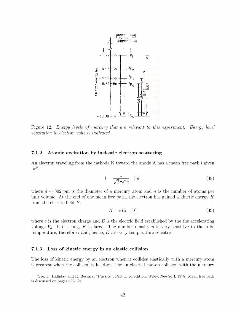
Figure 12: Energy levels of mercury that are relevant to this experiment. Energy levelseparation in electron volts is indicated.

7.1.2 Atomic excitation by inelastic electron scattering

An electron traveling from the cathode K toward the anode A has a mean free path l givenby8 :

l =1√

2πd2n[m] (48)

where d ∼ 302 pm is the diameter of a mercury atom and n is the number of atoms perunit volume. At the end of one mean free path, the electron has gained a kinetic energy Kfrom the electric field E:

K = eEl [J ] (49)

where e is the electron charge and E is the electric field established by the the acceleratingvoltage Va. If l is long, K is large. The number density n is very sensitive to the tubetemperature; therefore l and, hence, K are very temperature sensitive.

7.1.3 Loss of kinetic energy in an elastic collision

The loss of kinetic energy by an electron when it collides elastically with a mercury atomis greatest when the collision is head-on. For an elastic head-on collision with the mercury

8See, D. Halliday and R. Resnick, ”Physics”, Part 1, 3d edition, Wiley, NewYork 1978. Mean free pathis discussed on pages 522-524.

42

atom initially at rest, the change in electron energy is given by9:

∆K =4mM

(m+M)2K0 [J ] (50)

where m and M are the masses of an electron and a mercury atom and K0 is the initialelectron energy.

7.1.4 Ionization potential of mercury

The Franck Hertz tube can be connected such that the ionization potential of mercury canbe measured. In this case, the anode is connected so that the anode is maintained at anegative potential of a couple of volts with respect to the cathode. In this condition, itis energetically impossible for any electron to reach the anode. When the grid potentialis made positive with respect to the cathode, electrons are accelerated to the grid. Somepass to through the grid into the space between the the grid and the anode, but all areeventually puled back and collected by the grid. However, if the electrons enter the spacebetween the grid and anode have sufficient energy to ionize the mercury atoms, then theresulting positive mercury ions are drawn to the anode and a positive current is registered.The measure of the anode current as a function of the grid to cathode potential differenceyields a measure of the ionization potential. The first difficulty is to determine the optimaloven temperature. If the vapor pressure of the mercury is too low, then the electronsentering the grid-to-anode region with sufficient energy to cause ionization will have a smallprobability of collision (long mean free path) and the ion current collected by the anodewill be too low. If the vapor pressure of mercury is too high, then the electrons will sufferinelastic collisions in the space between the cathode and the grid as soon as they energyslightly exceed the energy required to raise mercury atoms to their first excited state andwill therefore never attain sufficient energy to cause ionization.

7.2 Experimental setup and procedure suggestion

In this experiment, we will use a version of the Franck Hertz tube Mounted on Front-Platewith Mercury Filling and Heating Chamber from Klinger KEP (Model KA6040-KA6041),the Franck Hertz tube control unit KA6045, read out by an digital oscilloscope. A copyof the operating manual for this device is available on the class web site, it describes theFranck Hertz tube, the power supply used in this experiment as well as suggestions for thedata taking.

The Franck-Hertz tube is contained within an oven, which is a metal box with a ther-mostatically controlled heater and terminals for connections to the tube. A thermometercan be inserted through a hole in the top of the oven. The tube has a parallel system ofelectrodes in order to produce a fairly uniform electric field. The distance between the fila-ment/cathode and the perforated grid is much larger than the mean free path of electronsthrough the mercury vapor under normal operating conditions. A platinum ribbon with a

9See K. Rossberg, ”A first course in Analytical Mechanics”, Wiley, New York, 1983. Collision of twoparticles is discussed on page 157-160

43

small barium-oxide spot serves as a direct heated cathode. An electrode connected withthe cathode limits the current and suppresses secondary and reflected electrons, making theelectric field more uniform. In order to avoid current leakage along the hot glass wall ofthe tube, a protective ceramic ring is fused in the glass as a feed-through to the counterelectrode. The tube is evacuated and coated inside with a getter which absorbs traces ofair that leaked in during the manufacturing process and over the lifetime of the tube.

Before making any connections, be sure you understand the circuit. Figure 13 showsthe setup used for this experiment, this figure is extracted from the manufacturer manual.The web site gives a list of important caution and tips that you should read before startingyour experiment. When using the scope, couple the channel to DC to provide a good zeropoint for voltage. Also we will use the 60 Hz functionality of the power supply to minimizetemperature correlated drifts of the measured voltages.

Figure 13: The Franck-Hertz tube and electrical connection used in this experiment.

7.3 Lab objectives

To measure the energy of the 1st excited state of Hg and the work function of the heatingfilament.For this lab, you are asked to:

- in the theory section, explain in at least ten full sentences how the Bohr model of theatoms explains the quantization of excited states,

- use both peaks and valleys of your data to extract your results,

- use the result of your linear regression, to present a residual plot of your data.


The following questions should help you prepare for this lab:

44

- What is an ion? What is an excited state of an atom? How do those two conceptscontrast? Which energy is larger ionization potential or first excited state, explain.

- Why does the Franck-Hertz apparatus have a cathode, anode and grid? Why is theretarding voltage needed to observe the Franck-Hertz effect?

- Considering that the energy of the first excited state of the mercury atom is about 5.0eV above that of the ground state, what is the maximum amount of energy that anelectron with 4.0 electron volts of kinetic energy can impart to a mercury atom withwhich it collides? Same question for a 6.0 eV electron.

- What is vapor pressure? How does it apply to the Franck-Hertz apparatus you aregoing to work with?

- What is the mean free path of electrons propagating in a gas (see equation 48) at 180oC? At this temperature, the vapor pressure of Mercury is 1.1728 kPa.

- Suppose a voltage V is maintained between a cathode and an anode. The cathodeand the anode are separated by a distance d = 10cm. Suppose and electron is releasedat rest from a filament attached to the cathode, the electron will be accelerated to theanode. At what distance d′ from the cathode will this electro reach an energy of 5 eVif V = 6V, 12V or 24V?

References

The discussion of theFranck-Hertz Effect is copied from:

- the HyperPhysics web site: http://hyperphysics.phy-astr.gsu.edu/Hbase/hph.html

- The lab manual of the Michigan University: http://instructor.physics.lsa.umich.edu/adv-labs/Franck Hertz/franck-hertz.pdf

- The Franck-Hertz experiment web page at MIT: http://web.mit.edu/8.13/www/07.shtml

- D. Preston and E. Dietz, The Art of Experimental Physics, Wiley, New York, 1991.

45

Documents

PHYS 371: Electrons Laboratory Laboratory Manualfrantz/phys371/manual371.pdf · PHYS 371: Electrons Laboratory Laboratory Manual ... 4 The ratio Charge-to-Mass of the electron 21