Phys 256B Project Report (Spring Quarter 2013):Artifacts of Molecular Dynamics

Nithin DhananjayanGrad Group:Biophysics, Department:Chemistry

University of California, Davisndhananj@ucdavis.edu

June 15, 2013

Abstract

To understand the non-linear behavior that algoritms that make time discrete add to simulations(in addition to the potentially non-linear behavior of what is being simulated) I compared Stromer-Verlet algorithm with Runge-Kutta Order 4 for both a harmonic oscillator and a harmonic oscillatorbouncing against a hard wall. I wanted to do this so that I can get a better understanding of thetypes of issues that people doing molecular dynamics run into, since many available codes (Amber,CHARMM, Gromacs) use some version of the Stromer-Verlet Algorithm (usually the Leap-Frogalgorithm). Although, I would like to study the cases where damping and noise are accountedfor, there was some non-linear behavior seen in Runge-Kutta 4 near the point where it becomesunstable. I isolated some the parameters and some return maps that seem to indicate an attractorof some kind that would be interesting to characterize.

1

2 BACKGROUND

1 Introduction

1.1 Motivation

The Stromer-Verlet algorithm is used my many molecular dynamics simulation packages. Thisincludes popular molecular simulation packages like Gromacs, Amber, and CHARMM. Although thereare different implementations: velocity explicit formulation, leap-frog formulation, and position-Verletformulations, these formulations can be proven to give the same results. They need slightly differentinitialization procedures with velocity explicit having the simplest initialization.

In addition, Stromer-Verlet has some nice properties given its simplicity that higher order systems,like Runge-Kuttta-4, do not have. Because of this, I wanted to make a comparison between twoalgorithms, Stromer-Verlet, and Ruge-Kutta-4 regarding the non-linear dynamics that they introduce(in additions to the dynamics that they are simulating). So my project is to explore what theseadditional dynamics are.

1.2 Why is it interesting?

Computational chemists make use of Molecular Dynamics to answer many questions about chemicalsystems that range from complicated periodic materials to a biological complex of molecules. I am,myself, working on a biological system known as NADH:Dehydrogenase, that acts as a chemical protonpump that is powered by electron transport from a higher reduction potential to lower reductionpotential. I wonder what we are sacrificing by using the Stromer-Verlet algorithm, and what we aregaining as over an explicit Runge-Kutta method.

1.3 Project Summary

Initially, I was interested in finding out about the artifacts that simulation algorithms can injectinto the simulation. Unfortunately, many of the artifacts that I had tried to track down were createdby subtle bugs in my code, having to do with how I initialized the algorithm, or the order in which Iupdated the variables.

In this report, I give some details about one artifact I still believe to real and would like to investigatefurther. At particular parameters I am able to see a structured loss of energy in the phase space plotof the Runge-Kutta 4 method, while the Stromer-Verlet remained stable. Following up on this case,I was able to isolate a set of points that show up in return maps of multiple periods. I believe goingthrough the whole ’learning channel’, studying this one case (which I did not find till late), would beinstructive.

2 Background

2.1 Molecular Dynamics

Molecular Dynamics software packages are used in computational biochemistry to answer basicquestions about conformations and placements about particular molecules in relation to each otherand to get order of magnitude estimates on the forces, energies, and free energies involved.

In order to do a simulation of this sort, molecular dynamics software packages simulate a discretetime version of Newton’s Laws working in response to a variety of bonded and non-bonded forces.Although, there are packages (sometimes called ab intio molecular dynamics, or QM-MM) that takeinto account quantum mechanics, even these packages use quantum mechanics only to create a static

Phys 256B Project Report 2 Nithin Dhananjayan

2.2 Gromacs as an example molecular dynamics package 2 BACKGROUND

potential created by electrons for the nuclei to move in for each time step (making use of the Born-Oppenheimer approximation). Because of this, I will only go into detail regarding the Newtonianparts of the simulation.

2.2 Gromacs as an example molecular dynamics package

One popular, and one of the fastest molecular dynamics simulation packages, is called Gromacs–which stands for GROningen MAchine for Chemical Simulations.

The basic algorithm that Gromacs follows is outlined below:

(i) compute accelerations in accordance with forces disregarding constraints, a(t)i = F

(t)imi

(ii) Update and scale velocities: v′(t) = λ(v(t−∆t) + a ∗∆t) where λ =[1 + ∆t

τt

(T0

T t− 12 ∆t− 1

)] 12

(iii) Compute new unconstrained positions: r′(t) = r(t−∆t) + v′(t)∆t(iv) Apply constraint solver: r′(t) → r′′(t)

(v) Adjust velocity based on constraints: v(t) = r′′(t)−rt−∆t

∆t

(vi) Scale coordinates and size of simulation box: r(t) = µr′′(t), b = µb, µ =[1 + ∆t

τpβ(P (t) − P0

)] 13

The scaling in step (ii) is for the purpose of applying a thermostat, to try to maintain constanttemperature. I will be using a different method because it is not clear that this method creates theproper use of time steps to keep the nice properties of Stromer-Verlet that I will talk about later.Also, for a single particle, applying a background ”noise” to simulate a ”heat bath” and a dampingfactor to simulate and implicit solvent is more appropriate.

The scaling in step (vi) is to apply a barostat to maintain a desired pressure. I will not be makingany adjustments to pressure, since this becomes quite confusing for a single particle case, and again,I am not sure how to maintain the nice properties of Stromer-Verlet when applying a barostat.

Constrains are another complication in Gromacs that I will be avoiding. The purpose of constraintsin a molecular dynmics simulation is to create infinitely stiff bonds without having forces that havevery steep curves. The time step required for a simulation is usually limited by how steep the potentialbeing simulated are. Also, very stiff bonds, like Carbon-Hydrogen bonds are usually not activated bythe temperatures typical in biology, and since our simulations don’t account for quantum mechanics,we would want to treat bonds like this as constraints rather than extremely stiff springs.

The forces that are usually involved in molecular dynamics are: (1) Harmonic forces use to simulatebonds, angles between two bonds, and dihedral angles. (2) long range electrostatic forces modeledby Coulomb forces. (3) r−12 potentials to model strong repulsive interactions without discontinuities,and (4) r−6 potentials to model dipole-dipole interactions.

2.3 Stability of Stromer-Verlet and Runge-Kutta

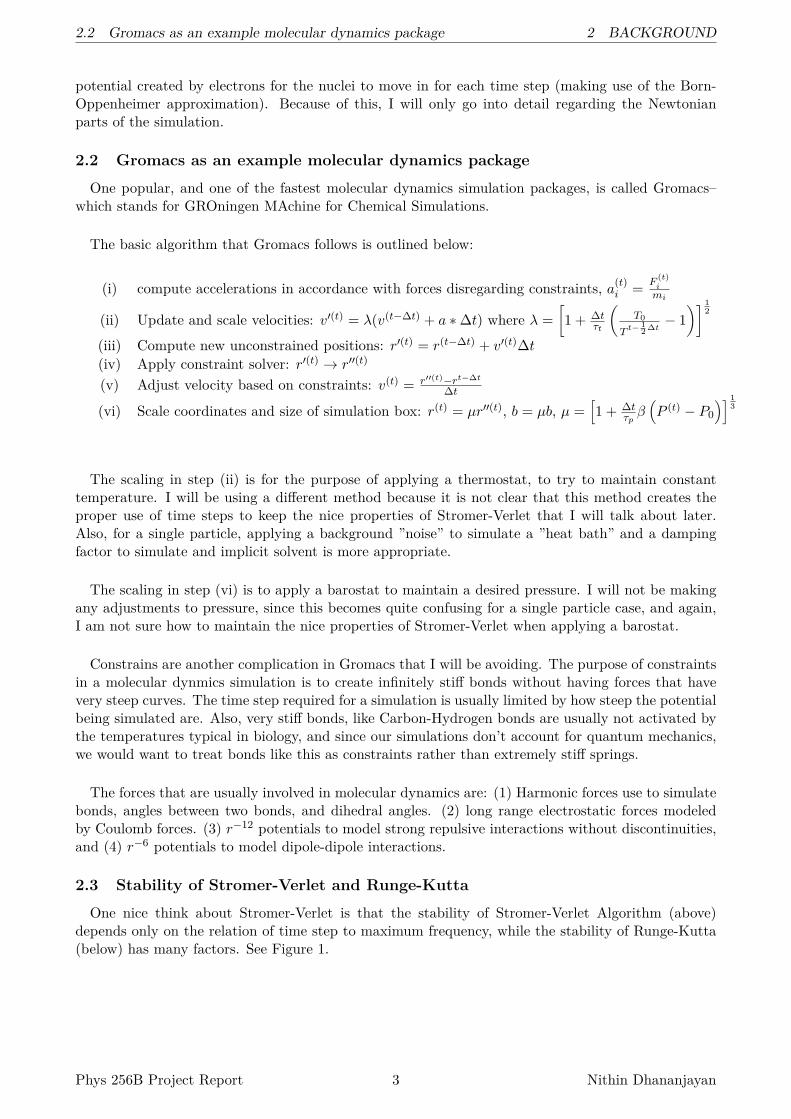
One nice think about Stromer-Verlet is that the stability of Stromer-Verlet Algorithm (above)depends only on the relation of time step to maximum frequency, while the stability of Runge-Kutta(below) has many factors. See Figure 1.

Phys 256B Project Report 3 Nithin Dhananjayan

2.3 Stability of Stromer-Verlet and Runge-Kutta 2 BACKGROUND

Figure 1: Stability of Stromer-Verlet Algorithm (above[2]) depends only on the relation of time stepto maximum frequency, while the stability of Runge-Kutta (below[3]) has many factors.

Phys 256B Project Report 4 Nithin Dhananjayan

3 DYNAMICAL SYSTEM

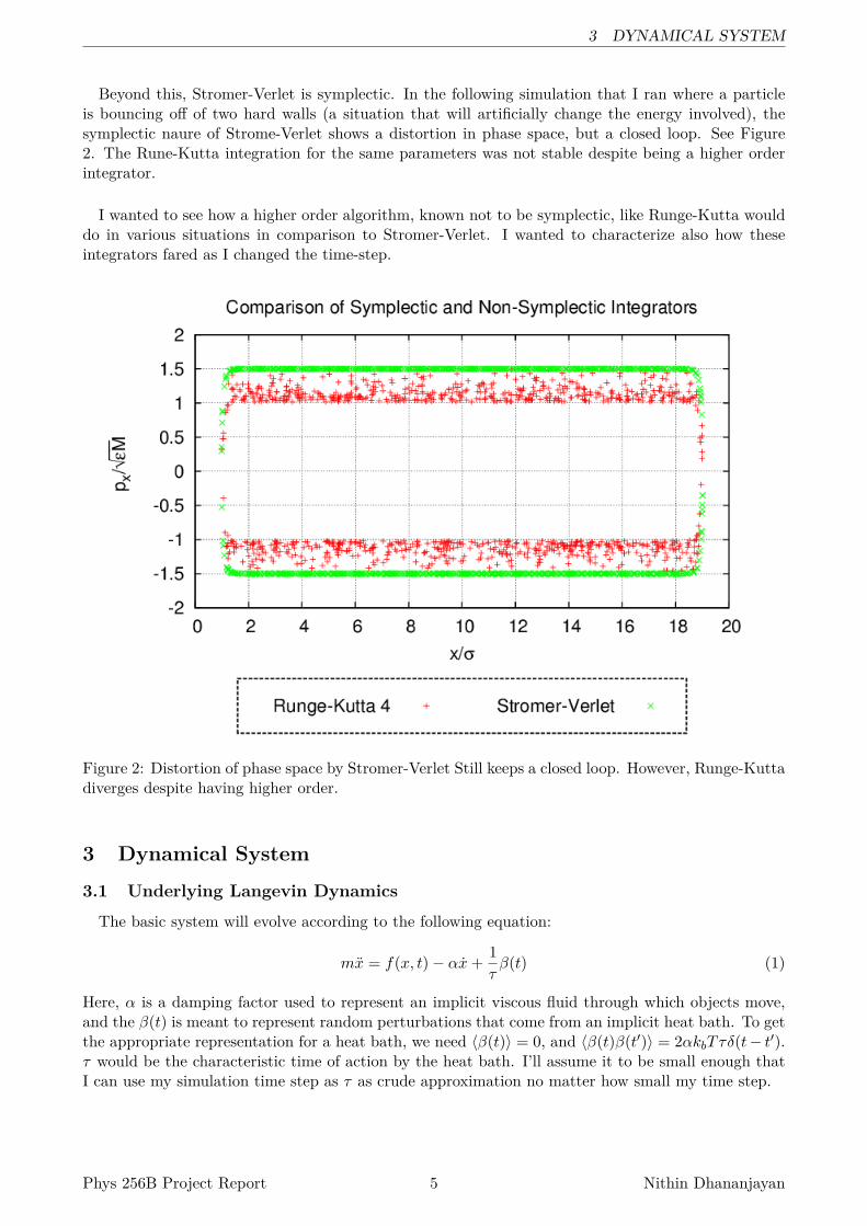
Beyond this, Stromer-Verlet is symplectic. In the following simulation that I ran where a particleis bouncing off of two hard walls (a situation that will artificially change the energy involved), thesymplectic naure of Strome-Verlet shows a distortion in phase space, but a closed loop. See Figure2. The Rune-Kutta integration for the same parameters was not stable despite being a higher orderintegrator.

I wanted to see how a higher order algorithm, known not to be symplectic, like Runge-Kutta woulddo in various situations in comparison to Stromer-Verlet. I wanted to characterize also how theseintegrators fared as I changed the time-step.

Figure 2: Distortion of phase space by Stromer-Verlet Still keeps a closed loop. However, Runge-Kuttadiverges despite having higher order.

3 Dynamical System

3.1 Underlying Langevin Dynamics

The basic system will evolve according to the following equation:

mx = f(x, t)− αx+ 1τβ(t) (1)

Here, α is a damping factor used to represent an implicit viscous fluid through which objects move,and the β(t) is meant to represent random perturbations that come from an implicit heat bath. To getthe appropriate representation for a heat bath, we need 〈β(t)〉 = 0, and 〈β(t)β(t′)〉 = 2αkbTτδ(t− t′).τ would be the characteristic time of action by the heat bath. I’ll assume it to be small enough thatI can use my simulation time step as τ as crude approximation no matter how small my time step.

Phys 256B Project Report 5 Nithin Dhananjayan

3.2 Model Systems 3 DYNAMICAL SYSTEM

3.2 Model Systems

The basic systems I want to look at are a harmonic oscillator and a harmonic oscillator bouncingagainst a hard-wall. To this end, I place the harmonic oscillator inside a box in such a way that I canmove the equilibrium position or change the initial velocity so that the system can easily be adjustedto be one of the two model systems I want to explore. The ”force field” for this underlying system is:

f = k(x− xeq) + 12εσ

[(σ

x

)13+(

σ

Lbox − x

)13]

(2)

The first term is the harmonic oscillator, with a k that can be set to zero to get rid of the spring,while the second term represents the walls. I made the simulator use natural units where ε and σ areused as units of energy and distance. So to get rid of the walls, I would need to comment that partout of my code.

3.3 Algorithms

In some sense, what the algorithms themselves are (was included in my presentation) matter lessthan what my actual implementation was.

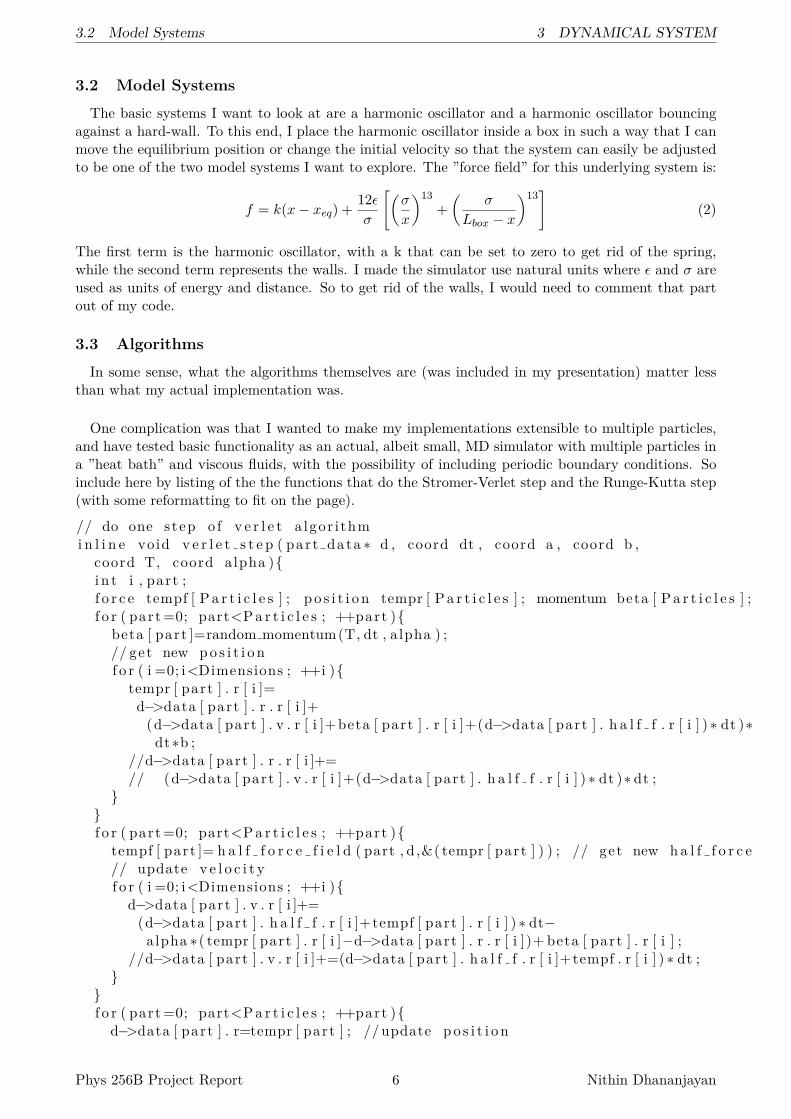
One complication was that I wanted to make my implementations extensible to multiple particles,and have tested basic functionality as an actual, albeit small, MD simulator with multiple particles ina ”heat bath” and viscous fluids, with the possibility of including periodic boundary conditions. Soinclude here by listing of the the functions that do the Stromer-Verlet step and the Runge-Kutta step(with some reformatting to fit on the page).

// do one step o f v e r l e t a lgor i thmi n l i n e void v e r l e t s t e p ( part data ∗ d , coord dt , coord a , coord b ,

coord T, coord alpha ){i n t i , part ;f o r c e tempf [ P a r t i c l e s ] ; p o s i t i o n tempr [ P a r t i c l e s ] ; momentum beta [ P a r t i c l e s ] ;f o r ( part =0; part<P a r t i c l e s ; ++part ){

beta [ part ]=random momentum(T, dt , alpha ) ;// get new p o s i t i o nf o r ( i =0; i<Dimensions ; ++i ){

tempr [ part ] . r [ i ]=d−>data [ part ] . r . r [ i ]+

(d−>data [ part ] . v . r [ i ]+ beta [ part ] . r [ i ]+(d−>data [ part ] . h a l f f . r [ i ] ) ∗ dt )∗dt∗b ;

//d−>data [ part ] . r . r [ i ]+=// (d−>data [ part ] . v . r [ i ]+(d−>data [ part ] . h a l f f . r [ i ] ) ∗ dt )∗ dt ;

}}f o r ( part =0; part<P a r t i c l e s ; ++part ){

tempf [ part ]= h a l f f o r c e f i e l d ( part , d ,&( tempr [ part ] ) ) ; // get new h a l f f o r c e// update v e l o c i t yf o r ( i =0; i<Dimensions ; ++i ){

d−>data [ part ] . v . r [ i ]+=(d−>data [ part ] . h a l f f . r [ i ]+tempf [ part ] . r [ i ] ) ∗ dt−

alpha ∗( tempr [ part ] . r [ i ]−d−>data [ part ] . r . r [ i ])+ beta [ part ] . r [ i ] ;//d−>data [ part ] . v . r [ i ]+=(d−>data [ part ] . h a l f f . r [ i ]+tempf . r [ i ] ) ∗ dt ;

}}f o r ( part =0; part<P a r t i c l e s ; ++part ){

d−>data [ part ] . r=tempr [ part ] ; // update p o s i t i o n

Phys 256B Project Report 6 Nithin Dhananjayan

3.3 Algorithms 3 DYNAMICAL SYSTEM

p b c c o r r e c t (&(d−>data [ part ] . r ) ) ;d−>data [ part ] . h a l f f=tempf [ part ] ; // update f o r c e

}}

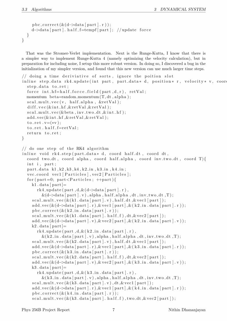
That was the Stromer-Verlet implementation. Next is the Runge-Kutta, I know that there isa simpler way to implement Runge-Kutta 4 (namely optimizing the velocity calculation), but inpreparation for including noise, I setup this more robust version. In doing so, I discovered a bug in theinitialization of my simpler version, and found that this new version can use much larger time steps.

// doing a time d e r i v i a t i v e o f so r t s , i gno r e the p o i t i o n s l o ti n l i n e s t ep data rk4 update ( i n t part , par t data ∗ d , p o s i t i o n ∗ r , v e l o c i t y ∗ v , coord alpha , coord ha l f a lpha , coord dt , coord inv two dt , coord T){

s t ep data t o r e t ;f o r c e i n t h f=h a l f f o r c e f i e l d ( part , d , r ) , r e tVal ;momentum beta=random momentum(T, dt , alpha ) ;s c a l m u l t v e c (v , ha l f a lpha , &retVal ) ;d i f f v e c (& i n t h f ,& retVal ,& retVal ) ;s c a l m u l t v e c (&beta , inv two dt ,& i n t h f ) ;add vec(& i n t h f ,& retVal ,& retVal ) ;t o r e t . v=(∗v ) ;t o r e t . h a l f f=retVal ;r e turn t o r e t ;

}

// do one step o f the RK4 algor i thmi n l i n e void rk4 s t ep ( par t data ∗ d , coord h a l f d t , coord dt ,

coord two dt , coord alpha , coord ha l f a lpha , coord inv two dt , coord T){i n t i , part ;par t data k1 , k2 , k3 , k4 , k2 in , k3 in , k4 in ;vec coord vec1 [ P a r t i c l e s ] , vec2 [ P a r t i c l e s ] ;f o r ( part =0; part<P a r t i c l e s ; ++part ){

k1 . data [ part ]=rk4 update ( part , d ,&(d−>data [ part ] . r ) ,

&(d−>data [ part ] . v ) , alpha , ha l f a lpha , dt , inv two dt ,T) ;s c a l m u l t v e c (&(k1 . data [ part ] . v ) , h a l f d t ,& vec1 [ part ] ) ;add vec (&(d−>data [ part ] . r ) ,& vec1 [ part ] ,&( k2 in . data [ part ] . r ) ) ;p b c c o r r e c t (&( k2 in . data [ part ] . r ) ) ;s c a l m u l t v e c (&(k1 . data [ part ] . h a l f f ) , dt ,& vec2 [ part ] ) ;add vec (&(d−>data [ part ] . v) ,& vec2 [ part ] ,&( k2 in . data [ part ] . v ) ) ;k2 . data [ part ]=

rk4 update ( part , d ,&( k2 in . data [ part ] . r ) ,&( k2 in . data [ part ] . v ) , alpha , ha l f a lpha , dt , inv two dt ,T) ;

s c a l m u l t v e c (&(k2 . data [ part ] . v ) , h a l f d t ,& vec1 [ part ] ) ;add vec (&(d−>data [ part ] . r ) ,& vec1 [ part ] ,&( k3 in . data [ part ] . r ) ) ;p b c c o r r e c t (&( k3 in . data [ part ] . r ) ) ;s c a l m u l t v e c (&(k2 . data [ part ] . h a l f f ) , dt ,& vec2 [ part ] ) ;add vec (&(d−>data [ part ] . v) ,& vec2 [ part ] ,&( k3 in . data [ part ] . v ) ) ;k3 . data [ part ]=

rk4 update ( part , d ,&( k3 in . data [ part ] . r ) ,&( k3 in . data [ part ] . v ) , alpha , ha l f a lpha , dt , inv two dt ,T) ;

s c a l m u l t v e c (&(k3 . data [ part ] . v ) , dt ,& vec1 [ part ] ) ;add vec (&(d−>data [ part ] . r ) ,& vec1 [ part ] ,&( k4 in . data [ part ] . r ) ) ;p b c c o r r e c t (&( k4 in . data [ part ] . r ) ) ;s c a l m u l t v e c (&(k3 . data [ part ] . h a l f f ) , two dt ,& vec2 [ part ] ) ;

Phys 256B Project Report 7 Nithin Dhananjayan

5 RESULTS

add vec (&(d−>data [ part ] . v) ,& vec2 [ part ] ,&( k4 in . data [ part ] . v ) ) ;k4 . data [ part ]=

rk4 update ( part , d ,&( k4 in . data [ part ] . r ) ,&( k4 in . data [ part ] . v ) , alpha , ha l f a lpha , dt , inv two dt ,T) ;

}f o r ( i =0; i<Dimensions ; ++i ){

f o r ( part =0; part<P a r t i c l e s ; ++part ){d−>data [ part ] . h a l f f . r [ i ]=

( k1 . data [ part ] . h a l f f . r [ i ]+2.0∗ k2 . data [ part ] . h a l f f . r [ i ]+2 .0∗ k3 . data [ part ] . h a l f f . r [ i ]+k4 . data [ part ] . h a l f f . r [ i ] ) / 6 . 0 ;

}f o r ( part =0; part<P a r t i c l e s ; ++part ){

d−>data [ part ] . r . r [ i ]+=dt ∗( k1 . data [ part ] . v . r [ i ]+2.0∗ k2 . data [ part ] . v . r [ i ]+

2 .0∗ k3 . data [ part ] . v . r [ i ]+k4 . data [ part ] . v . r [ i ] ) / 6 . 0 ;p b c c o r r e c t (&(d−>data [ part ] . r ) ) ;

}f o r ( part =0; part<P a r t i c l e s ; ++part ){

d−>data [ part ] . v . r [ i ]+=two dt∗d−>data [ part ] . h a l f f . r [ i ] ;}

}}

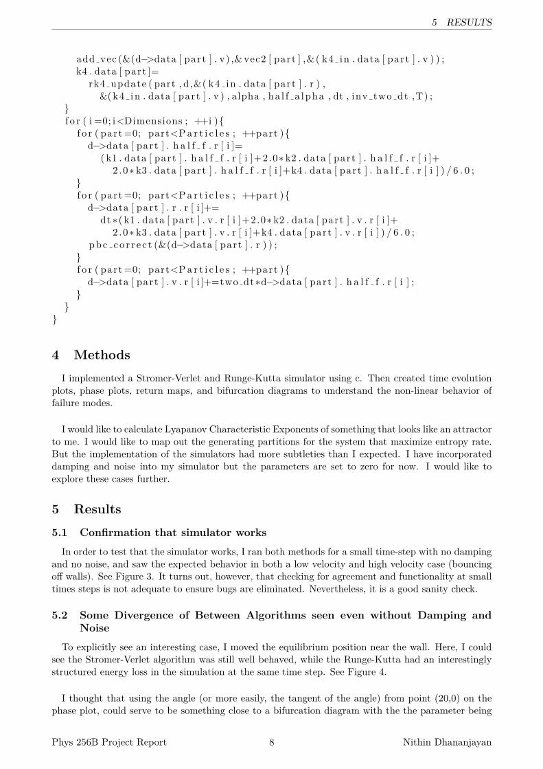
4 Methods

I implemented a Stromer-Verlet and Runge-Kutta simulator using c. Then created time evolutionplots, phase plots, return maps, and bifurcation diagrams to understand the non-linear behavior offailure modes.

I would like to calculate Lyapanov Characteristic Exponents of something that looks like an attractorto me. I would like to map out the generating partitions for the system that maximize entropy rate.But the implementation of the simulators had more subtleties than I expected. I have incorporateddamping and noise into my simulator but the parameters are set to zero for now. I would like toexplore these cases further.

5 Results

5.1 Confirmation that simulator works

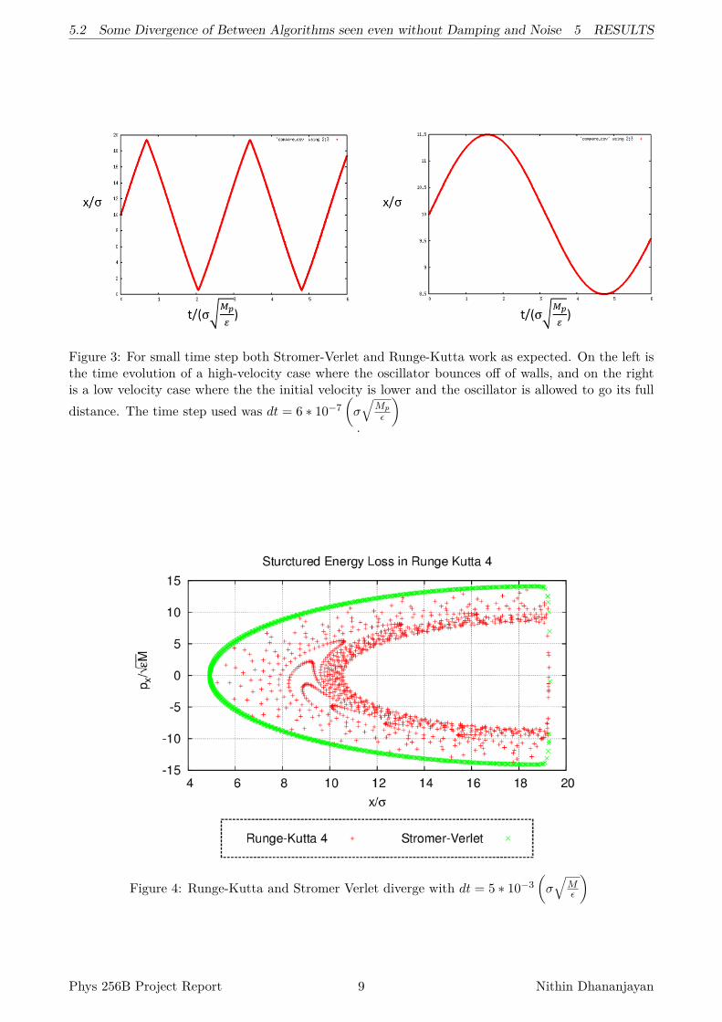
In order to test that the simulator works, I ran both methods for a small time-step with no dampingand no noise, and saw the expected behavior in both a low velocity and high velocity case (bouncingoff walls). See Figure 3. It turns out, however, that checking for agreement and functionality at smalltimes steps is not adequate to ensure bugs are eliminated. Nevertheless, it is a good sanity check.

5.2 Some Divergence of Between Algorithms seen even without Damping andNoise

To explicitly see an interesting case, I moved the equilibrium position near the wall. Here, I couldsee the Stromer-Verlet algorithm was still well behaved, while the Runge-Kutta had an interestinglystructured energy loss in the simulation at the same time step. See Figure 4.

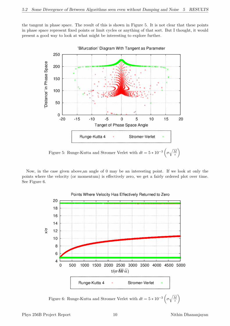
I thought that using the angle (or more easily, the tangent of the angle) from point (20,0) on thephase plot, could serve to be something close to a bifurcation diagram with the the parameter being

Phys 256B Project Report 8 Nithin Dhananjayan

5.2 Some Divergence of Between Algorithms seen even without Damping and Noise 5 RESULTS

Figure 3: For small time step both Stromer-Verlet and Runge-Kutta work as expected. On the left isthe time evolution of a high-velocity case where the oscillator bounces off of walls, and on the rightis a low velocity case where the the initial velocity is lower and the oscillator is allowed to go its fulldistance. The time step used was dt = 6 ∗ 10−7

(σ√

Mp

ε

).

Figure 4: Runge-Kutta and Stromer Verlet diverge with dt = 5 ∗ 10−3(σ√

Mε

)

Phys 256B Project Report 9 Nithin Dhananjayan

5.2 Some Divergence of Between Algorithms seen even without Damping and Noise 5 RESULTS

the tangent in phase space. The result of this is shown in Figure 5. It is not clear that these pointsin phase space represent fixed points or limit cycles or anything of that sort. But I thought, it wouldpresent a good way to look at what might be interesting to explore further.

Figure 5: Runge-Kutta and Stromer Verlet with dt = 5 ∗ 10−3(σ√

Mε

)

Now, in the case given above,an angle of 0 may be an interesting point. If we look at only thepoints where the velocity (or momentum) is effectively zero, we get a fairly ordered plot over time.See Figure 6.

Figure 6: Runge-Kutta and Stromer Verlet with dt = 5 ∗ 10−3(σ√

Mε

)

Phys 256B Project Report 10 Nithin Dhananjayan

6 CONCLUSIONS

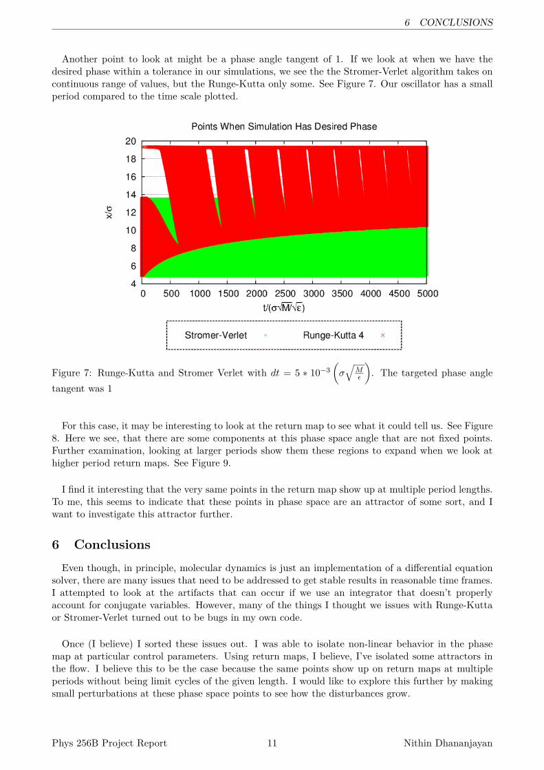
Another point to look at might be a phase angle tangent of 1. If we look at when we have thedesired phase within a tolerance in our simulations, we see the the Stromer-Verlet algorithm takes oncontinuous range of values, but the Runge-Kutta only some. See Figure 7. Our oscillator has a smallperiod compared to the time scale plotted.

Figure 7: Runge-Kutta and Stromer Verlet with dt = 5 ∗ 10−3(σ√

Mε

). The targeted phase angle

tangent was 1

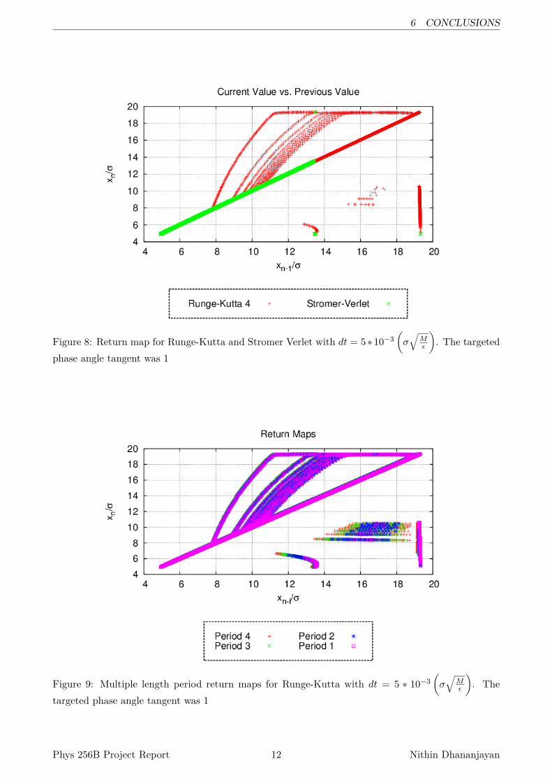
For this case, it may be interesting to look at the return map to see what it could tell us. See Figure8. Here we see, that there are some components at this phase space angle that are not fixed points.Further examination, looking at larger periods show them these regions to expand when we look athigher period return maps. See Figure 9.

I find it interesting that the very same points in the return map show up at multiple period lengths.To me, this seems to indicate that these points in phase space are an attractor of some sort, and Iwant to investigate this attractor further.

6 Conclusions

Even though, in principle, molecular dynamics is just an implementation of a differential equationsolver, there are many issues that need to be addressed to get stable results in reasonable time frames.I attempted to look at the artifacts that can occur if we use an integrator that doesn’t properlyaccount for conjugate variables. However, many of the things I thought we issues with Runge-Kuttaor Stromer-Verlet turned out to be bugs in my own code.

Once (I believe) I sorted these issues out. I was able to isolate non-linear behavior in the phasemap at particular control parameters. Using return maps, I believe, I’ve isolated some attractors inthe flow. I believe this to be the case because the same points show up on return maps at multipleperiods without being limit cycles of the given length. I would like to explore this further by makingsmall perturbations at these phase space points to see how the disturbances grow.

Phys 256B Project Report 11 Nithin Dhananjayan

6 CONCLUSIONS

Figure 8: Return map for Runge-Kutta and Stromer Verlet with dt = 5∗10−3(σ√

Mε

). The targeted

phase angle tangent was 1

Figure 9: Multiple length period return maps for Runge-Kutta with dt = 5 ∗ 10−3(σ√

Mε

). The

targeted phase angle tangent was 1

Phys 256B Project Report 12 Nithin Dhananjayan

7 BIBLIOGRAPHY

7 Bibliography

1. Crutchfield, J.P. “Lecture Notes” Natural Computation and Self-Organization Winter/Spring2013

2. C. C. Strelioff and J. P. Crutchfield, ”Optimal Instruments and Models for Noisy Chaos”, CHAOS17 (2007) 043127. Santa Fe Institute Working Paper 06-11-042. arxiv.org e-print cs.LG/0611054.

3. GROMACS: A message-passing parallel molecular dynamics implementation, H.J.C. Berendsen,D. van der Spoel, R. van Drunen, Computer Physics Communications 91 (1995) 43-56

4. A simple and effective Verlet-type algorithm for simulating Langevin Dynamics, Neils Gronbach-Jensen, Oded Farago, Molecular Physics 2013

5. Suli, Endre; Mayers, David (2003), An Introduction to Numerical Analysis, Cambridge Univer-sity Press, ISBN 0-521-00794-1.

6. http://en.wikipedia.org/wiki/Runge%E2%80%93Kutta methods

Phys 256B Project Report 13 Nithin Dhananjayan