Important points

• Spherical (convex or concave) mirrorsform images that are magnified andat a different location than the origi-nals.

• Images for concave mirrors are real,while convex-mirror images are vir-tual.

Important equations

• Spherical mirror

1/s + 1/s′ = 1/ f

f = R/2

• Magnification

m = y′/y

= −s′/s

1 One way to remember convex vs. con-cave is that concave mirrors form a“cave”, or hollowed out surface, by curv-ing inward.

PHYS 202 Notes, Week 9Greg Christian

March 22 & 24, 2016Last updated: 03/24/2016 at 12:23:56

This week we learn about images by mirrors, refraction, and thin lenses.

Images

Spherical Mirrors

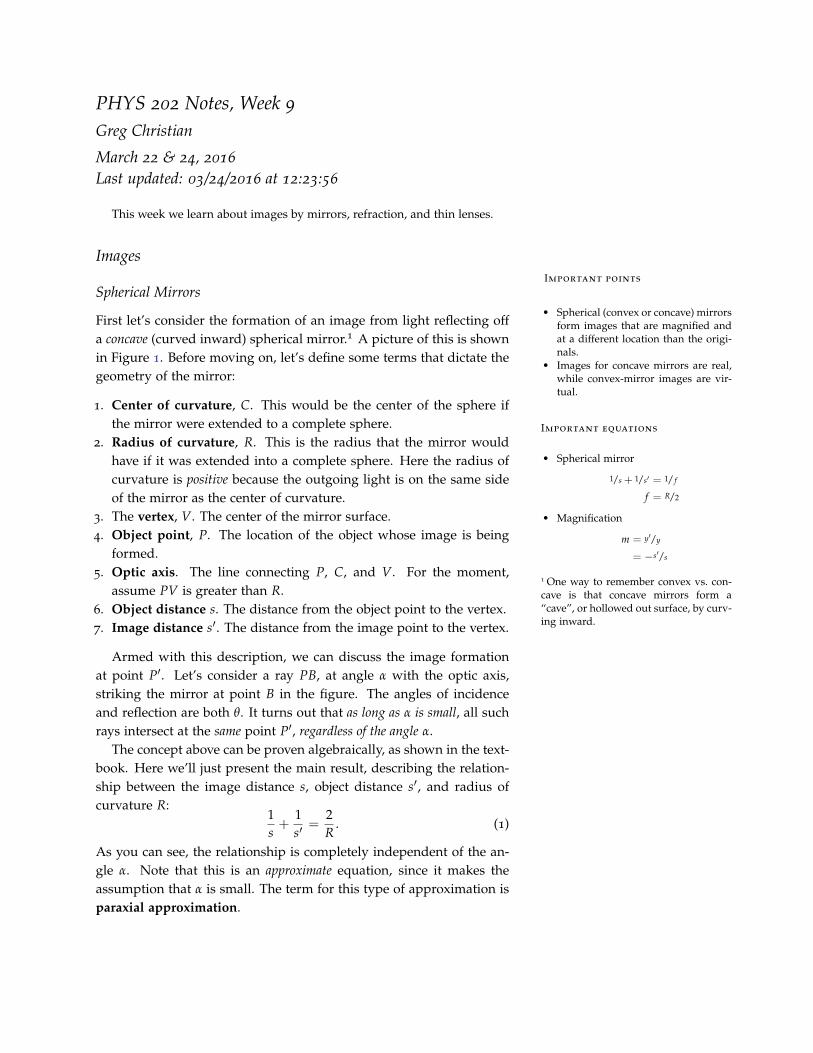
First let’s consider the formation of an image from light reflecting offa concave (curved inward) spherical mirror.1 A picture of this is shownin Figure 1. Before moving on, let’s define some terms that dictate thegeometry of the mirror:

1. Center of curvature, C. This would be the center of the sphere ifthe mirror were extended to a complete sphere.

2. Radius of curvature, R. This is the radius that the mirror wouldhave if it was extended into a complete sphere. Here the radius ofcurvature is positive because the outgoing light is on the same sideof the mirror as the center of curvature.

3. The vertex, V. The center of the mirror surface.4. Object point, P. The location of the object whose image is being

formed.5. Optic axis. The line connecting P, C, and V. For the moment,

assume PV is greater than R.6. Object distance s. The distance from the object point to the vertex.7. Image distance s′. The distance from the image point to the vertex.

Armed with this description, we can discuss the image formationat point P′. Let’s consider a ray PB, at angle α with the optic axis,striking the mirror at point B in the figure. The angles of incidenceand reflection are both θ. It turns out that as long as α is small, all suchrays intersect at the same point P′, regardless of the angle α.

The concept above can be proven algebraically, as shown in the text-book. Here we’ll just present the main result, describing the relation-ship between the image distance s, object distance s′, and radius ofcurvature R:

1s+

1s′

=2R

. (1)

As you can see, the relationship is completely independent of the an-gle α. Note that this is an approximate equation, since it makes theassumption that α is small. The term for this type of approximation isparaxial approximation.

phys 202 notes, week 9 2

Figure 1: Image formation from a con-cave spherical mirror.

Because the light rays really do converge at point P′, this is an ex-ample of a real image. Contrast with the virtual image formed by aplane mirror, which only had apparent convergence behind the mirror.

When dealing with spherical mirrors, we can define something calledthe focal point, F, which is the image point formed when the objectis “infinitely” far away from the mirror, i.e. when s → ∞. We call thedistance to the focal point the focal length, f . This can be derived fromEq. (1):

1∞

+1f=

2R

(2)

⇒ f =R2

. (3)

Note that f > 0 for a concave mirror. For a convex mirror, f < 0.Equation (1) is usually written in terms of the focal length f rather

than the radius R. In this form, it becomes

1s+

1s′

=1f

. (4)

Magnification

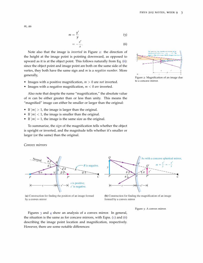
As shown in Figure 2, the height of a finite object is not the same at theobject point (point P) as at the image point (point P′). This leads to thephenomenon of magnification. Assuming some object has height y atthe object point and Y′ at the image point, we can define magnification,

phys 202 notes, week 9 3

Figure 2: Magnification of an image dueto a concave mirror.

m, as

m =y′

y(5)

= − s′

s. (6)

Note also that the image is inverted in Figure 2: the direction ofthe height at the image point is pointing downward, as opposed toupward as it is at the object point. This follows naturally from Eq. (6):since the object point and image point are both on the same side of thevertex, they both have the same sign and m is a negative number. Moregenerally,

• Images with a positive magnification, m > 0 are not inverted.• Images with a negative magnification, m < 0 are inverted.

Also note that despite the name “magnification,” the absolute valueof m can be either greater than or less than unity. This means the“magnified” image can either be smaller or larger than the original:

• If |m| > 1, the image is larger than the original.• If |m| < 1, the image is smaller than the original.• If |m| = 1, the image is the same size as the original.

To summarize, the sign of the magnification tells whether the objectis upright or inverted, and the magnitude tells whether it’s smaller orlarger (or the same) than the original.

Convex mirrors

Figure 3: A convex mirror.

Figures 3 and 4 show an analysis of a convex mirror. In general,the situation is the same as for concave mirrors, with Eqns. (1) and (6)describing the image point location and magnification, respectively.However, there are some notable differences:

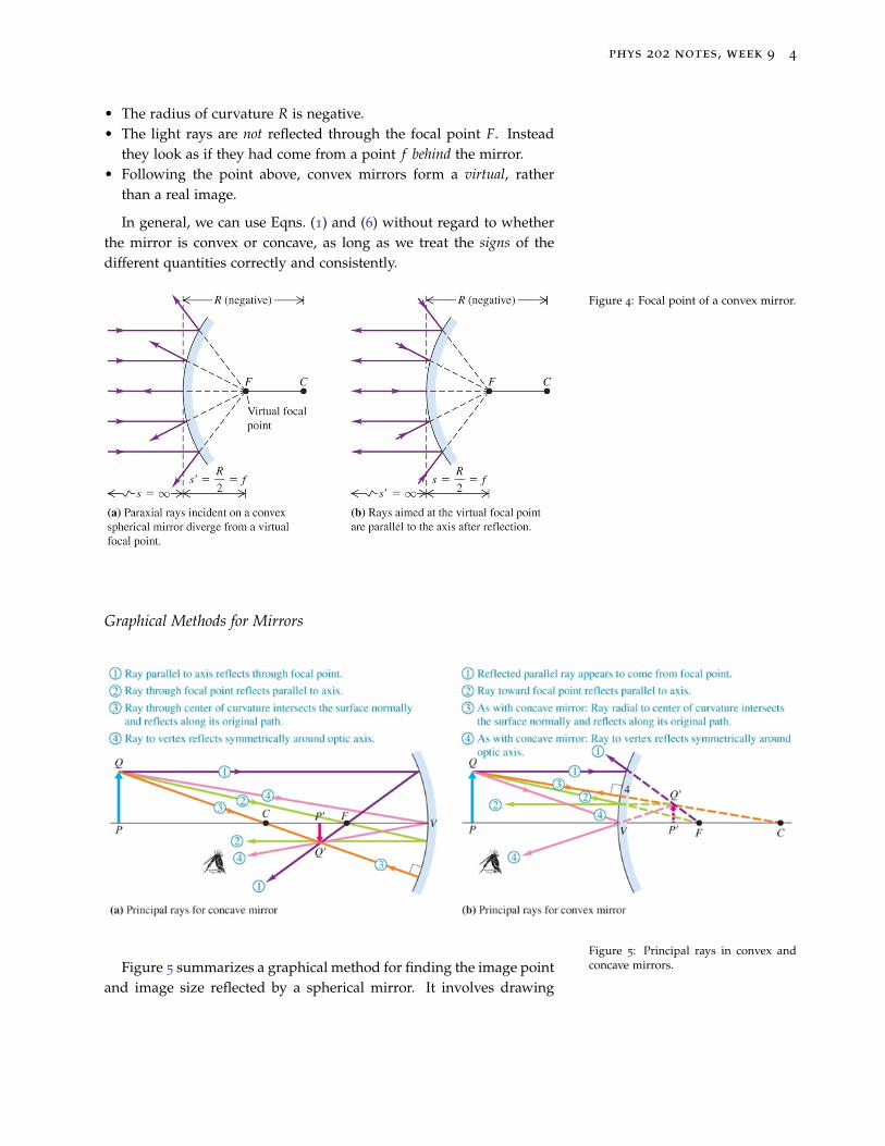
phys 202 notes, week 9 4

• The radius of curvature R is negative.• The light rays are not reflected through the focal point F. Instead

they look as if they had come from a point f behind the mirror.• Following the point above, convex mirrors form a virtual, rather

than a real image.

In general, we can use Eqns. (1) and (6) without regard to whetherthe mirror is convex or concave, as long as we treat the signs of thedifferent quantities correctly and consistently.

Figure 4: Focal point of a convex mirror.

Graphical Methods for Mirrors

Figure 5: Principal rays in convex andconcave mirrors.Figure 5 summarizes a graphical method for finding the image point

and image size reflected by a spherical mirror. It involves drawing

phys 202 notes, week 9 5

Important points

• Spherical refracting surfaces can beanalyzed in terms of the radius ofcurvature, similar to spherical mir-rors.

• The same equations can be used toanalyze lenses as mirrors, but younust take care to pay attention to thesigns of quantities.

Important equations

• Spherical refraction image point

na/s + nb/s′ = (nb−na)/R

• Spherical refraction magnification

m = −nas′/nbs

• Thin lens equation

1/ f = 1/s + 1/s′ (7)

= (n− 1) (1/R1 − 1/R2) (8)

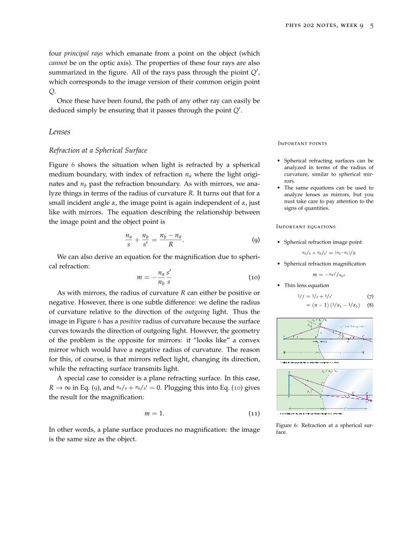
Figure 6: Refraction at a spherical sur-face.

four principal rays which emanate from a point on the object (whichcannot be on the optic axis). The properties of these four rays are alsosummarized in the figure. All of the rays pass through the pioint Q′,which corresponds to the image version of their common origin pointQ.

Once these have been found, the path of any other ray can easily bededuced simply be ensuring that it passes through the point Q′.

Lenses

Refraction at a Spherical Surface

Figure 6 shows the situation when light is refracted by a sphericalmedium boundary, with index of refraction na where the light origi-nates and nb past the refraction bnoundary. As with mirrors, we ana-lyze things in terms of the radius of curvature R. It turns out that for asmall incident angle α, the image point is again independent of α, justlike with mirrors. The equation describing the relationship betweenthe image point and the object point is

na

s+

nbs′

=nb − na

R. (9)

We can also derive an equation for the magnification due to spheri-cal refraction:

m = −na

nb

s′

s(10)

As with mirrors, the radius of curvature R can either be positive ornegative. However, there is one subtle difference: we define the radiusof curvature relative to the direction of the outgoing light. Thus theimage in Figure 6 has a positive radius of curvature because the surfacecurves towards the direction of outgoing light. However, the geometryof the problem is the opposite for mirrors: it “looks like” a convexmirror which would have a negative radius of curvature. The reasonfor this, of course, is that mirrors reflect light, changing its direction,while the refracting surface transmits light.

A special case to consider is a plane refracting surface. In this case,R→ ∞ in Eq. (9), and na/s + nb/s′ = 0. Plugging this into Eq. (10) givesthe result for the magnification:

m = 1. (11)

In other words, a plane surface produces no magnification: the imageis the same size as the object.

phys 202 notes, week 9 6

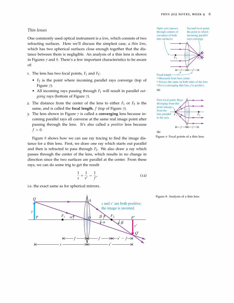
Figure 7: Focal points of a thin lens.

Thin lenses

One commonly used optical instrument is a lens, which consists of tworefracting surfaces. Here we’ll discuss the simplest case, a thin lens,which has two spherical surfaces close enough together that the dis-tance between them is negligible. An analysis of a thin lens is shownin Figures 7 and 8. There’s a few important characteristics to be awareof:

1. The lens has two focal points, F1 and F2:

• F2 is the point where incoming parallel rays converge (top ofFigure 7).

• All incoming rays passing through F1 will result in parallel out-going rays (bottom of Figure 7).

2. The distance from the center of the lens to either F1 or F2 is thesame, and is called the focal length, f (top of Figure 7).

3. The lens shown in Figure 7 is called a converging lens because in-coming parallel rays all converse at the same real image point afterpassing through the lens. It’s also called a positive lens becausef > 0.

Figure 8 shows how we can use ray tracing to find the image dis-tance for a thin lens. First, we draw one ray which starts out paralleland then is refracted to pass through F2. We also draw a ray whichpasses through the center of the lens, which results in no change indirection since the two surfaces are parallel at the center. From theserays, we can do some trig to get the result:

1s+

1s′

=1f

, (12)

i.e. the exact same as for spherical mirrors.

Figure 8: Analysis of a thin lens.

phys 202 notes, week 9 7

Figure 9: A diverging thin lens.

2 See the textbook for a derivation; wewon’t repeat it here.

Similarly, the magnification is the same as for mirrors:

m =y′

y= − s′

s. (13)

Essentially you can apply the exact same equations, but still musttake care to pay attention to the signs of the quantities to get the correctresults.

In addition to the converging lens already mentioned, we can alsodeal with diverging lenses. An example is shown in Figure 9. Hereincoming parallel rays diverge, or spread out after the lens. In thiscase, the focal points are flipped relative to the converging lens:

• F2 appears in front of the lens, at the point where parallel incidentrays look like they’re diverging from.

• F1 appears behind the lens, at the point there emergent parallel rayswould converge if the lens wasn’t there.

As a result, the focal length of a diverging lens is negative. For thisreason, it’s sometimes called a negative lens because f < 0.

Equations (12) and (13) apply equally well to diverging lenses. How-ever, take care to use the correct signs, in particular to remember thatf is a negative quantity for diverging lenses.

Thin Lens Equation

Figure 10: Illustration of lens geometryused in the lensmaker’s equation.

So far, we’ve seen Eq. (12) describing the image distance in termsof the focal length and object distance. Similar to mirrors, we can alsoexpress f in terms of the lens geometry and index of refraction. Thisis called the lensmaker’s equation. As an example, consider the lensshown in Figure 10. The focal length can be expressed as2

1f= (n− 1)

(1

R1− 1

R2

), (14)

phys 202 notes, week 9 8

where n is the index of refraction of the lens and the radii R1 and R2

are as shown in Figure 10.From this, we can write down what is called the thin lens equation,

fully describing the image distance in terms of the lens geometry andobject distance:

1s+

1s′

=1f

(15)

= (n− 1)(

1R1− 1

R2

). (16)

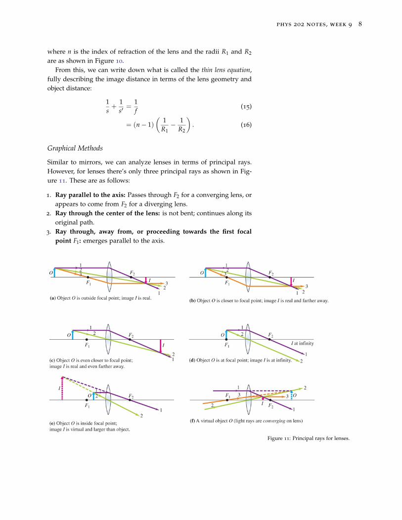
Graphical Methods

Similar to mirrors, we can analyze lenses in terms of principal rays.However, for lenses there’s only three principal rays as shown in Fig-ure 11. These are as follows:

1. Ray parallel to the axis: Passes through F2 for a converging lens, orappears to come from F2 for a diverging lens.

2. Ray through the center of the lens: is not bent; continues along itsoriginal path.

3. Ray through, away from, or proceeding towards the first focalpoint F1: emerges parallel to the axis.

Figure 11: Principal rays for lenses.