Embed Size (px)
Citation preview

Physics 1210
Lab Book
Spring 2018
Instructor: Brad Lyke
Created by and used with permission from:
Dr. Kobulnicky

Physics 1210 Experiments
Physics 1210
General guidelines for experiment reports
1) Reports should be typed and include tables and graphs, as appropriate, to demonstrate the
work and support the conclusions.
2) Reports should include the full names of all persons contributing to the work.
3) Matlab scripts used to make plots or do computations should be included as an appendix
4) There are no particular font or margins or pages requirements
5) A complete report should include:
An Abstract stating the main goal, the methods, and the main result or finding. Include
numerical results and their uncertainties (if calculated) in this section as well.
A short Introduction describing why the experiment is being performed, and the physics
concepts in use.
A Methods & Data section that describes the experimental setup in both words and with
appropriate graphics. This section may also include formulae or derivations needed to
demonstrate the objectives of the experiment. The Data section should also include
tables of data or derived parameters with appropriate units.
An Analysis section interpreting the data. This section may also talk about the precision
of the results achieved and the main sources of error or uncertainty. This section should
include graphs or figures that help interpret the data. Equations or derivations using basic
data to compute other parameters may also be included here. If a lab calls for a derivation
or extensive calculation, it will appear in this section. All data interpretation should be in
this section (graphs, calculations, etc).
A Results & Conclusions section describing what worked well or what could be changed
to achieve better results in the future if the equipment or the goals were slightly different.
An Appendix (or Appendices), which includes work performed but perhaps not essential
to the main body of the report. Things such as Matlab scripts used to make plots should
be included in the Appendix.
6) Feel free to include a digital photo of pertinent aspects of your setup or equipment.
Drawings are often better as they can be labeled to show sizes, distances, etc. All drawings or
photos MUST be original.
7) The text of the report should follow standard English grammar, punctuation and sentence
structure.
8) Grading of experimental reports will follow the rubric distributed to the class.
9) An example of a well-written report will be posted to the website.

Physics 1210 Experimental Report Grading Rubric
0 1 2 3 4
Poor Excellent
Abstract and overall: Does the abstract
state clearly the purpose and results of
the experiment? Does the report
conform to standard English sentence
structure and grammar usage? – 10%
Introduction: Does it contain a brief
background of why the experiment is
being performed and the relevant
physical principles or equations? –
20%
Methods & Data: Does the methods
section show figure(s) illustrating the
experimental setup and clearly
describe the procedure followed? Are
the fundamental relationships
explained in equations that stem from
fundamental physics principles? Does
the data section include tables
summarizing the individual
measurements, include multiple
measurements to reduce random error,
as needed, averages are computed, and
any needed figures to show the data or
its relation to an underlying physical
principle or hypothesis? – 20%
Analysis: Does the analysis show
original thought? Does it all (or
examples of all) calculations used
throughout the experiment? Does it
include diagrams for vectors, forces,
energy, etc. where those are
calculated? – 20%
Results and Conclusions: Are the
results succinctly stated, along with an
analysis of the errors or uncertainties
and how they affect the final result?
This section should also include what
was learned from re-doing the
experiment after any changes were put
into place. Are questions posted in the
Experiment Handout answered
completely and correctly? – 20%
Is the work, overall, neat and legible
and does it show original thought and
understanding (or is the work copied
from a friend or a solutions manual?) –
10%
Experiment 0 - Numerical Review
Name: _____________________
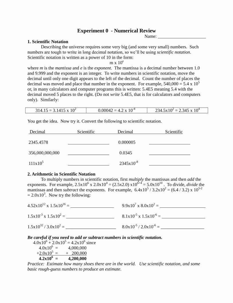
1. Scientific Notation
Describing the universe requires some very big (and some very small) numbers. Such
numbers are tough to write in long decimal notation, so we’ll be using scientific notation.
Scientific notation is written as a power of 10 in the form:
m x 10e
where m is the mantissa and e is the exponent. The mantissa is a decimal number between 1.0
and 9.999 and the exponent is an integer. To write numbers in scientific notation, move the
decimal until only one digit appears to the left of the decimal. Count the number of places the
decimal was moved and place that number in the exponent. For example, 540,000 = 5.4 x 10⁵
or, in many calculators and computer programs this is written: 5.4E5 meaning 5.4 with the
decimal moved 5 places to the right. (Do not write 5.4E5, that is for calculators and computers
only). Similarly:
314.15 = 3.1415 x 10² 0.00042 = 4.2 x 10
-4 234.5x10
2 = 2.345 x 10
4
You get the idea. Now try it. Convert the following to scientific notation.
Decimal Scientific Decimal Scientific
2345.4578 __________________ 0.000005 __________________
356,000,000,000 __________________ 0.0345 __________________
111x105 __________________ 2345x10
-8 __________________
2. Arithmetic in Scientific Notation
To multiply numbers in scientific notation, first multiply the mantissas and then add the
exponents. For example, 2.5x106 x 2.0x10
4 = (2.5x2.0) x10
6+4 = 5.0x10
10 . To divide, divide the
mantissas and then subtract the exponents. For example, 6.4x10⁵ / 3.2x10
2 = (6.4 / 3.2) x 10
5-2
= 2.0x10³. Now try the following:
4.52x1012
x 1.5x1016
= ___________________ 9.9x107 x 8.0x10
2 = ____________________
1.5x10-3
x 1.5x102 = _____________________ 8.1x10
-5 x 1.5x10
-6 = ___________________
1.5x1032
/ 3.0x102 = ______________________ 8.0x10
-5 / 2.0x10
-6 = ___________________
Be careful if you need to add or subtract numbers in scientific notation. 4.0x10
6 + 2.0x10
5 = 4.2x10
6 since
4.0x106 = 4,000,000
+2.0x105 = + 200,000
4.2x106 = 4,200,000
Practice: Estimate how many shoes there are in the world. Use scientific notation, and some
basic rough-guess numbers to produce an estimate.

3. Converting Units
Often we make a measurement in one unit (such as meters) but some other unit is desired
for a computation or answer (such as kilometers). You can use the tables in the Appendix of your
textbook to find handy conversion factors from one unit to another.
Example: You have 2340000000000 meters. How many kilometers is this?
There are 1000 m/km. Because kilometers are larger than meters, we need fewer of them to
specify the same distance, so divide the number of meters by the number of meters per kilometer
and notice how the units cancel out and leave you with the desired result.
Another way to think about this operation, is that you want fewer km than m, so just move the
decimal place three to the left since there are 103 m per kilometer. Or, if the new desired unit is
smaller, and you expect more of them, then multiply. For example, how many cm are there in 42
km?
Use the information in the appendix of your text to convert the following.
2 year = _____________________ s 1000 feet= _______________________ m
50 km = _____________________ m 3x10⁶ m = _______________________ cm
52,600,000 km = ______________ m 3450 seconds = ___________________ minute
6.0x10¹⁸
m = _________________ mm 600 hours = _______________________ days
5.2x10¹²
kg = _________________ g 365 days = _______________________ s
99 minutes = ________________ hr 1200 days = ______________________ yr

4. Angles and Trigonometry
Science and engineering is filled with examples where we need to use trig functions to
determine angles or sides of triangles, or to compute the projection of one vector onto another.
Solve for the unknown side or angle in the following triangles as review and practice.
5. Vector Addition
Vectors allow us to specify directions in two or three dimensions by expressing a
direction as the sum of direction along two or more axes. In two dimensions, we let be the unit
vector in the X-direction and is the unit vector in Y-direction, and then r is the vector sum of the
X- and Y-components. See the first example below for an instance of vector addition, and then
complete the two vector addition problems, drawing the individual vectors and the total vector in
each case, following the example.
3.5m
φ
2.1m
θ
θ
α
β
γ
δ
6. Measurement and Uncertainties
Very few measurements are direct measurements. Length, perhaps, is a direct
measurement, when one uses a well-calibrated comparison tool of a standard length. Most
measurements, such as mass and temperature are indirect; they depend on intermediate
measurements and apparatuses and a subsequent calculation. For many students it comes as a
surprise that absolutely exact measurements are impossible. If we weigh a small piece of
material on a balance, a typical result could be 1.7438 grams. This is, however, only an
approximation to the true weight, just as the value 3.1416 is only an approximation to the
number π. A more sensitive balance would give a more accurate number. This is true of all
measurements. Measurements always are imprecise, that is, there is some inherent uncertainty
(we use the word uncertainty rather than error in most cases, as error implies a mistake) in the
measurement, no matter how careful we try to be. In any kind of science or engineering, getting
the right answer is usually the easy part; calculating how certain you are of that answer, i.e., what
is the uncertainty on your answer, is the hard part, and an important part. The uncertainties
reflect both the precision of the measurement/measurer and the accuracy of the instrument.
The degree of precision with which an observer can read a given linear scale depends
upon the definiteness of the marks on the scale and the skill with which the observer can estimate
fractional parts of scale division. In many instruments of precision, the linear scale is provided
with some sort of vernier, which is a mechanical substitute for the estimation of fractional parts
of scale divisions. Its use requires skill and judgment.
The degree of accuracy is determined by how close we can expect to be to the true or
actual value. For instance, when we measure the length of a small object, we should expect that a
meter stick will give a less accurate answer than a micrometer, provided that both instruments
have been calibrated well.
A common way of increasing the accuracy of a measurement done with an instrument of
a given precision is to repeat a measurement many times under identical circumstances and then
build an experimental average.
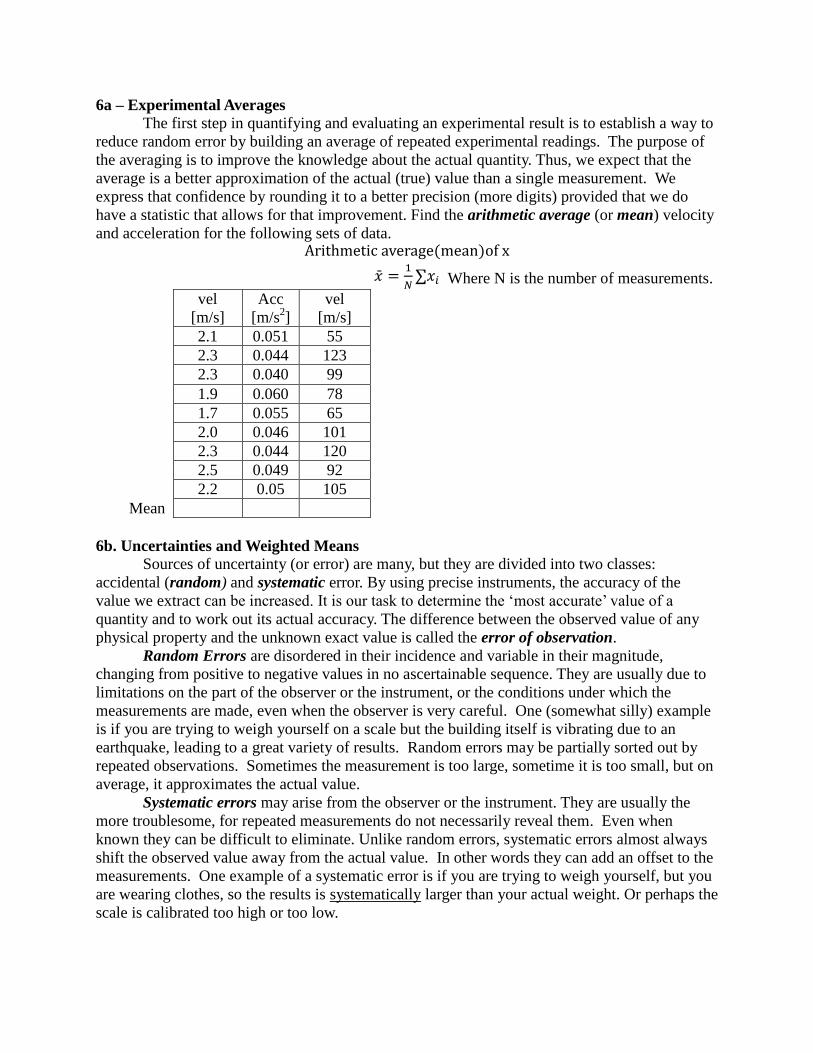
6a – Experimental Averages
The first step in quantifying and evaluating an experimental result is to establish a way to
reduce random error by building an average of repeated experimental readings. The purpose of
the averaging is to improve the knowledge about the actual quantity. Thus, we expect that the
average is a better approximation of the actual (true) value than a single measurement. We
express that confidence by rounding it to a better precision (more digits) provided that we do
have a statistic that allows for that improvement. Find the arithmetic average (or mean) velocity
and acceleration for the following sets of data.
vel
[m/s]
Acc
[m/s2]
vel
[m/s]
2.1 0.051 55
2.3 0.044 123
2.3 0.040 99
1.9 0.060 78
1.7 0.055 65
2.0 0.046 101
2.3 0.044 120
2.5 0.049 92
2.2 0.05 105
6b. Uncertainties and Weighted Means
Sources of uncertainty (or error) are many, but they are divided into two classes:
accidental (random) and systematic error. By using precise instruments, the accuracy of the
value we extract can be increased. It is our task to determine the ‘most accurate’ value of a
quantity and to work out its actual accuracy. The difference between the observed value of any
physical property and the unknown exact value is called the error of observation.
Random Errors are disordered in their incidence and variable in their magnitude,
changing from positive to negative values in no ascertainable sequence. They are usually due to
limitations on the part of the observer or the instrument, or the conditions under which the
measurements are made, even when the observer is very careful. One (somewhat silly) example
is if you are trying to weigh yourself on a scale but the building itself is vibrating due to an
earthquake, leading to a great variety of results. Random errors may be partially sorted out by
repeated observations. Sometimes the measurement is too large, sometime it is too small, but on
average, it approximates the actual value.
Systematic errors may arise from the observer or the instrument. They are usually the
more troublesome, for repeated measurements do not necessarily reveal them. Even when
known they can be difficult to eliminate. Unlike random errors, systematic errors almost always
shift the observed value away from the actual value. In other words they can add an offset to the
measurements. One example of a systematic error is if you are trying to weigh yourself, but you
are wearing clothes, so the results is systematically larger than your actual weight. Or perhaps the
scale is calibrated too high or too low.
Where N is the number of measurements.
Mean
There are all kinds of systematic errors. As another example, let’s take a look at a
hypothetical sequence of values made for the gravitational acceleration on earth: 9.78, 9.81,
9.81, 9.79, 12.5, 9.80 [m/s2]. It seems quite possible that some mistake was made in recording
’12.5’ and it is reasonable to exclude that value from further analysis. It represents an obvious
systematic error. There is no absolute limit for which we may assume that the above is the case.
For our undergraduate lab we want to keep records of all data and exclude outliers only if they
are off the average of the remaining data by 100% or more and only if we have just one outlier.
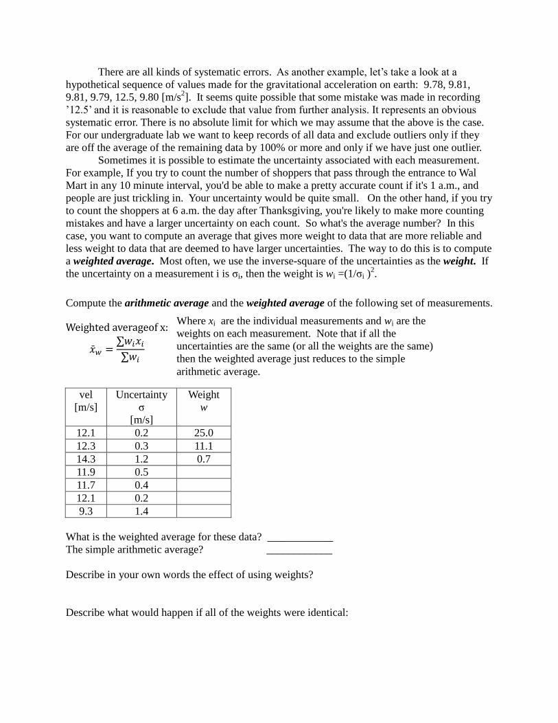
Sometimes it is possible to estimate the uncertainty associated with each measurement.
For example, If you try to count the number of shoppers that pass through the entrance to Wal
Mart in any 10 minute interval, you'd be able to make a pretty accurate count if it's 1 a.m., and
people are just trickling in. Your uncertainty would be quite small. On the other hand, if you try
to count the shoppers at 6 a.m. the day after Thanksgiving, you're likely to make more counting
mistakes and have a larger uncertainty on each count. So what's the average number? In this
case, you want to compute an average that gives more weight to data that are more reliable and
less weight to data that are deemed to have larger uncertainties. The way to do this is to compute
a weighted average. Most often, we use the inverse-square of the uncertainties as the weight. If
the uncertainty on a measurement i is σi, then the weight is wi =(1/σi )2.
Compute the arithmetic average and the weighted average of the following set of measurements.
vel
[m/s]
Uncertainty
σ
[m/s]
Weight
w
12.1 0.2 25.0
12.3 0.3 11.1
14.3 1.2 0.7
11.9 0.5
11.7 0.4
12.1 0.2
9.3 1.4
What is the weighted average for these data? ____________
The simple arithmetic average? ____________
Describe in your own words the effect of using weights?
Describe what would happen if all of the weights were identical:
Where xi are the individual measurements and wi are the
weights on each measurement. Note that if all the
uncertainties are the same (or all the weights are the same)
then the weighted average just reduces to the simple
arithmetic average.
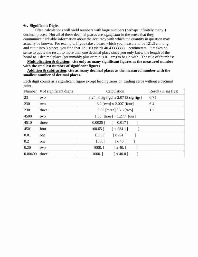
6c. Significant Digits
Often calculations will yield numbers with large numbers (perhaps infinitely many!)
decimal places. Not all of these decimal places are significant in the sense that they
communicate reliable information about the accuracy with which the quantity in question may
actually be known. For example, if you take a board which you measure to be 121.3 cm long
and cut it into 3 pieces, you find that 121.3/3 yields 40.43333333... centimeters. It makes no
sense to quote the result to more than one decimal place since you only knew the length of the
board to 1 decimal place (presumably plus or minus 0.1 cm) to begin with. The rule of thumb is:
Multiplication & division: cite only as many significant figures as the measured number
with the smallest number of significant figures.
Addition & subtraction: cite as many decimal places as the measured number with the
smallest number of decimal places.
Each digit counts as a significant figure except leading zeros or trailing zeros without a decimal
point.
Number # of significant digits Calculation Result (in sig figs)
23 two 3.24 [3 sig figs] x 2.07 [3 sig figs] 6.71
230 two 3.2 [two] x 2.007 [four] 6.4
230. three 5.55 [three] / 3.3 [two] 1.7
4500 two 1.05 [three] + 1.277 [four]
4510 three 0.0025 [ ] – 0.017 [ ]
4501 four 100.65 [ ] + 234.1 [ ]
0.01 one 1005 [ ] x 231 [ ]
0.2 one 1000 [ ] x 40 [ ]
0.20 two 1000. [ ] x 40. [ ]
0.00400 three 1000. [ ] x 40.0 [ ]

6d. Experimental Error and Data Scatter
Another step in quantifying and evaluating an experimental result is to establish a way to
describe the scatter or dispersion in the data due to random error. The first way to build such a
measure of data dispersion is called the standard deviation, defined as σ
where N is the number of data points, is the arithmetic average, and xi is each of the individual
data points. Find the mean and the standard deviation for the data set in the table below:
vel [m/s]
2.1
2.3
2.3
1.9
1.7
2.0
2.3
2.5
1.9
2
2.2
1.9
1.8
=
σ =
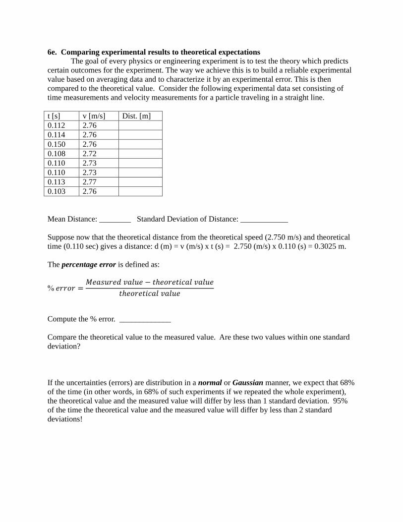
6e. Comparing experimental results to theoretical expectations
The goal of every physics or engineering experiment is to test the theory which predicts
certain outcomes for the experiment. The way we achieve this is to build a reliable experimental
value based on averaging data and to characterize it by an experimental error. This is then
compared to the theoretical value. Consider the following experimental data set consisting of
time measurements and velocity measurements for a particle traveling in a straight line.
t [s] v [m/s] Dist. [m]
0.112 2.76
0.114 2.76
0.150 2.76
0.108 2.72
0.110 2.73
0.110 2.73
0.113 2.77
0.103 2.76
Mean Distance: ________ Standard Deviation of Distance: ____________
Suppose now that the theoretical distance from the theoretical speed (2.750 m/s) and theoretical
time (0.110 sec) gives a distance: d (m) = v (m/s) x t (s) = 2.750 (m/s) x 0.110 (s) = 0.3025 m.
The percentage error is defined as:
Compute the % error. _____________
Compare the theoretical value to the measured value. Are these two values within one standard
deviation?
If the uncertainties (errors) are distribution in a normal or Gaussian manner, we expect that 68%
of the time (in other words, in 68% of such experiments if we repeated the whole experiment),
the theoretical value and the measured value will differ by less than 1 standard deviation. 95%
of the time the theoretical value and the measured value will differ by less than 2 standard
deviations!
Dis
tance
Time (s)
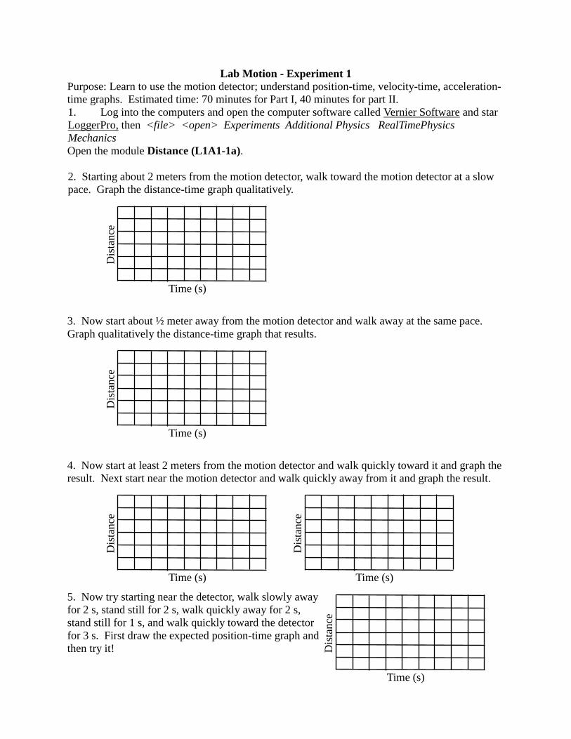
Lab Motion - Experiment 1
Purpose: Learn to use the motion detector; understand position-time, velocity-time, acceleration-
time graphs. Estimated time: 70 minutes for Part I, 40 minutes for part II.
1. Log into the computers and open the computer software called Vernier Software and star
LoggerPro, then <file> <open> Experiments Additional Physics RealTimePhysics
Mechanics
Open the module Distance (L1A1-1a).
2. Starting about 2 meters from the motion detector, walk toward the motion detector at a slow
pace. Graph the distance-time graph qualitatively.
3. Now start about ½ meter away from the motion detector and walk away at the same pace.
Graph qualitatively the distance-time graph that results.
4. Now start at least 2 meters from the motion detector and walk quickly toward it and graph the
result. Next start near the motion detector and walk quickly away from it and graph the result.
5. Now try starting near the detector, walk slowly away
for 2 s, stand still for 2 s, walk quickly away for 2 s,
stand still for 1 s, and walk quickly toward the detector
for 3 s. First draw the expected position-time graph and
then try it!
Dis
tance
Time (s)
Dis
tance
Time (s)
Dis
tance
Time (s)
Dis
tance
Time (s)
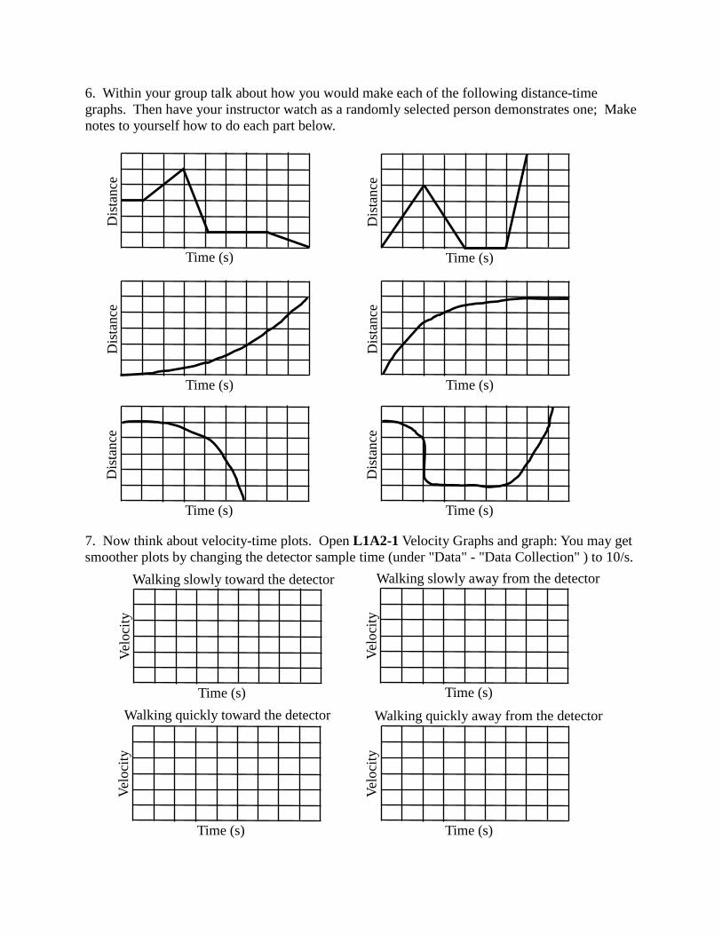
6. Within your group talk about how you would make each of the following distance-time
graphs. Then have your instructor watch as a randomly selected person demonstrates one; Make
notes to yourself how to do each part below.
7. Now think about velocity-time plots. Open L1A2-1 Velocity Graphs and graph: You may get
smoother plots by changing the detector sample time (under "Data" - "Data Collection" ) to 10/s.
Vel
oci
ty
Time (s)
Vel
oci
ty
Time (s)
Vel
oci
ty
Time (s)
Vel
oci
ty
Time (s)
Walking slowly toward the detector Walking slowly away from the detector
Walking quickly toward the detector Walking quickly away from the detector
Dis
tance
Time (s)
Dis
tance
Time (s)
Dis
tance
Time (s)
Dis
tance
Time (s)
Dis
tance
Time (s)
Dis
tance
Time (s)

8. Talk about with your group and sketch a velocity-time graph if you were to
walk toward the detector slowly for 2 s
stand still for 1 s
walk quickly away for 2 s
walk slowly away for 2 s
Try it out and verify your prediction.
9. Open Velocity from Position (L1A3-1). Study the position-time graph below and sketch
quantitatively the corresponding velocity-time graph. Then try it out. Did it match?
When each person can do this, demonstrate it for your instructor and have them initial. ___
They may want to ask you things like “How can you tell from a position-time graph that you are
moving at a constant speed?” or “How does the position time graph change if you move faster?”
Vel
oci
ty
Time (s)
0 1 2 3 4 5 6 7 8 9
Time (s)
D
ista
nce
(m
)
-2
-1
0
1
2
0 1 2 3 4 5 6 7 8 9
Time (s)
V
eloci
ty (
m/s
)
-2
-1
0
1
2
0 1 2 3 4 5 6 7 8 9
Time (s)
D
ista
nce
(m
)
-2
-1
0
1
2
0 1 2 3 4 5 6 7 8 9
Time (s)
V
eloci
ty (
m/s
)
-2
-1
0
1
2
Now have your instructor draw a velocity-time graph and your group tries to predict the position-
time graph. Then perform the motion and graph it with the motion detector.
Your instructor will ask something like “On the basis of just the velocity-time graph, can you tell
where you end up?” Can you tell how far you've moved? If so, how can you tell?”
10. As a group come up with a way to make an object accelerate, an object for which you can
measure its motion using the motion detector (suggestion: rolling an object down a slope tends to
work better than dropping an object). You may get better graphs by increasing the sample rate to
30/s.
Discuss and sketch
what do you expect
the velocity-time and
position-time graph to
look like for your
experiment. Dropping
objects onto the
motion detector can
damage them, so be
careful, or come up
with some method that
does not involve
dropping.
When you have agreed
on an experimental
approach, describe it
to your instructor for
their ok and have them initial. _______
0 1 2 3 4 5 6 7 8 9
Time (s)
D
ista
nce
(m
)
-2
-1
0
1
2
0 1 2 3 4 5 6 7 8 9
Time (s)
V
eloci
ty (
m/s
)
-2
-1
0
1
2
11. Describe briefly your experiment below.
Test your plan by using the motion detector to make a position-time and a velocity-time plot.
Print out your actual v-t and x-t plots and affix them below (or save a jpeg and email it to your
whole group). You can use the cursor to measure points on your graph fairly precisely.
How might you measure the acceleration by using these plots? Show below how you compute
the acceleration and then show your instructor. _______
0 1 2 3 4 5 6 7 8 9
Time (s)
D
ista
nce
(m
)
-2
-1
0
1
2
0 1 2 3 4 5 6 7 8 9
Time (s)
V
eloci
ty (
m/s
)
-2
-1
0
1
2
Use the software module called "Speeding Up (L2A1-1)" to re-perform your experiment and
show the acceleration-time plot along with the v-t and x-t plot. Print out and affix these below
and annotate them to describe what you are seeing. You may need to limit the sample time to
just a fraction of a second and plot that part.
How did your computed acceleration compare with the graphed one here? Show how you
computed the acceleration.
Dis
tance
(m
)
-2 -1
0
1
2
0 1 2 3 4 5 6 7 8 9
Time (s)
A
ccel
erat
ion (
m/s
2)
-2
-1
0
1
2
V
eloci
ty (
m/s
)
-2
-1
0
1
2
0 1 2 3 4 5 6 7 8 9
Time (s)
0 1 2 3 4 5 6 7 8 9
Time (s)

12. Given the following acceleration-time curve, try to predict the v-t and x-t curve. Do you
have to assume that your object starts from rest? Do you have to assume that your object starts at
x=0?
Assuming that the objects starts at v=0, x=0, find the final velocity and the final position. Show
how you do this. Instructor initial at end of section. _________
0 1 2 3 4 5 6 7 8 9
Time (s)
D
ista
nce
(m
)
-2
-1
0
1
2
0 1 2 3 4 5 6 7 8 9
Time (s)
V
eloci
ty (
m/s
)
-2
-1
0
1
2
0 1 2 3 4 5 6 7 8 9
Time (s)
A
ccel
erat
ion (
m/s
2)
-2
-1
0
1
2

Part II
13. Devise an experiment to measure g. Show whether g is the same or different for a massive
object or a less massive object. Also show whether g is the same acting over a big distance
versus a small distance. There are many ways to do this. You need not even use any fancy
equipment. Concentrate on simplicity and accuracy. When you have a plan, describe it to your
instructor for approval and initial. ________ Then go conduct your experiment. Be sure to ask
if you would like equipment or tools that you don't see available in the room.
Perform your experiment as many times as you like to obtain results that you trust. Collect data
carefully as you will need to write up a formal experimental paper describing your purpose, your
method, your data, and your results. Turn in a report on your experiment using the provided
example Experimental Report as a template. Include a Matlab graph of the position of your
dropped object versus time as it falls from the roof. Include a digital photo of pertinent
equipment or events in your experiment. Include an estimate of the % error in your
measurement of g.
Be sure to include details of all of your equipment used. Feel free to ask for advice. It is
possible to be very precise with your measurement of g if sufficient attention to detail and
measurement is achieved! Practicing your method ahead of time can significantly reduce
measurement errors.
Please turn in the rubric on pg. 4 at the beginning of the manual with your report.
Lab Projectiles – Experiment 2
In this experiment, your team will fire a projectile at a given random angle to hit an intended
target accurately. Your instructor will show you the experimental setup. In brief, the rules are:
1) You pick the muzzle velocity (one, two, or three clicks of the spring-loaded cannon).
2) You will be given a standard cannonball.
3) You may test fire the cannon with any launch angle, but the final angle will be given to you.
4) You pick the target location and the launch location.
5) You may test fire your cannon as many times as you like on your tabletop without letting
the cannonball hit the tabletop or the floor.
6) The projectile must be fired from the table and land on the floor.
7) When you fire for real, you only get one shot. If you fail to hit the paper target on the
ground a new angle will be given to you and you will have to recompute the range. We will
use carbon paper underneath a target piece of paper to record the distance from the intended
landing site.
8) Think and measure carefully. The most accurate groups often land within 3 cm of the target
location!!
When you have a strategy for computing the landing location, discuss your intended launch plan
and your plan to compute the landing location with your instructor and have them initial. Make
sure that everyone in your group can explain the procedure that will be used. ________
Launch angle 1: _________ Instructor initials: __________
Launch angle 2: _________ Instructor initials: __________
Report guidelines
1) Be sure to include in your report a diagram of the experimental setup with any necessary
measurements and other details, such as masses, distances, etc.
2) Include a set of calculations (can be handwritten if done neatly) that shows your
theoretical target location and how you arrived at this number. What other things did you
have to measure to estimate your intended target location? No guessing allowed. Make
careful measurements and document everything!
3) Include a Matlab plot that shows the landing location as a function of θ, where θ is the
launch angle above the horizontal. You will only be given one θ for your real launch, but
your graph will nicely show how distance varies with θ given your fixed values of launch
velocity and initial height.
4) After your experimental test firing, you will have a chance to assess your results and
fix/remedy any mistakes that you can identify. If something went wrong, include an
analysis of where the problem occurred. Then, document any changes you made and re-
perform the experiment to show that you have caught and fixed any mistakes.
Equipment
Spring-launched cannon, standard cannonball, meter sticks, paper, carbon paper, c-clamps.
Please turn in the rubric at the beginning of the manual with your report.
Lab Springs – Experiment 3
Part I – Measure a spring constant. Make several measurements with tools you already know as
you stretch the spring several different distances. Make a Matlab plot to show the force required
as a function of distance and fit a reasonable looking function to your data. Take as much data as
you need to get a reliable result, using the best practices that you already know.
Hints:
1) The more data points you have the better the Matlab fit will be.
2) Remember to measure an unweighted length.
3) Do not use many similar masses. Try using some very large and very small masses.
When you have your data, show your instructor your method and have them initial. _______
Integrate this curve to show how much energy is stored in the spring and make a plot of energy
stored in your spring versus distance. This involves doing an integral. Show the calculations in
the Analysis section of your experiment report. If you want a challenge, I'll show you how to do
a numerical integral in Matlab (optional). The report for this experiment only covers part I.
Part II is not part of the experiment. Something for part II will be included at the end of
the report, however.
Equipment:
Large spring, rod, rod clamps, standard mass set, meter sticks, laptop (provided in lab)
Part II – Devise a workout. The guidelines are that your workout must
1) Consume at least 400 Calories (1 Calorie = 4186 J) of work for one individual person,
you!!! (If this seems too easy because you're a superstar, you are welcome to go for more
Calories.)
2) Have a peak power output of at least 300 W for some 30-sec duration or longer (or go for
more W if you are a superstar.)
3) Consist of at least 3 and not more than 6 activities from the following lists
4) Where needed, adopt the mass of a 70 kg person (or use your own mass if you wish).
5) Muscles are only about 33% efficient, meaning that the Calories required are actually
about three times greater than the actual mechanical work achieved. Compute your
mechanical work in the strict physics sense, and the multiply by a factor of 3 to find the
Calories used.
Group I – These are activities are relatively easy to figure out the work required. Pick most or
all of your activities from this list.
A. Lifting weights (either free or simple machine weights). You can do several of these in
your workout (e.g., bench, curls, leg press, etc) but it counts as one activity.
B. Climbing stairs (or stepping repeatedly onto a box) or the stair climber machine.
C. Squats or similar (note, you do as much work going down as up, why? Also with pushups,
etc.)
D. Pushups, pull-ups, or similar
E. Walking/running (ask for help as the work you do here is mostly against gravity; on
average, walking 1 mile burns about 110 Calories). Look for information on how to
calculate this on the internet. Calories burned are dependent on walking/running speed.
F. Shuttle relay (suicides; where you run back and forth, changing your kinetic energy many
times)
Group II – These are activities it is a challenge to compute the work/power for. Pick at most one
activity from this list. If you use a machine at a gym that calculates Calories burned, cite the
machine.
A. Rowing machine with variable resistance
B. Stationary bike with variable resistance
C. Elliptical trainer
D. Swimming
E. Ask about others that you may want to invent.
First sketch out your workout plan and have your instructor initial to approve the basic plan.
Instructor initials: _________
After the end of the full experimental report for part I, include a short section for part II. Show
calculations for each of your proposed activities to demonstrate how much work you do in each
activity, and your average power during the activity. Show explicitly how the peak power in W
is achieved. Summarize your workout in a table showing the activity, the work done, the average
power, and the time of each activity. This short writeup is separate from the spring report in part
I. It is not a full experimental report. A couple paragraphs and a couple tables (with some
calculations) should be enough.
If you actually do your workout, on your honor, add in your report how easy or hard, doable or
undoable each phase exercise was and how you would modify your workout based on what you
experienced.
For 5 extra credit points, get at least 2/3 of your group to go do your workout together. Again, on
your honor. I trust you. Mention it in your short writeup mentioned above.
Please turn in the rubric at the beginning of the manual with your report.
Lab Engineering – Experiment 4
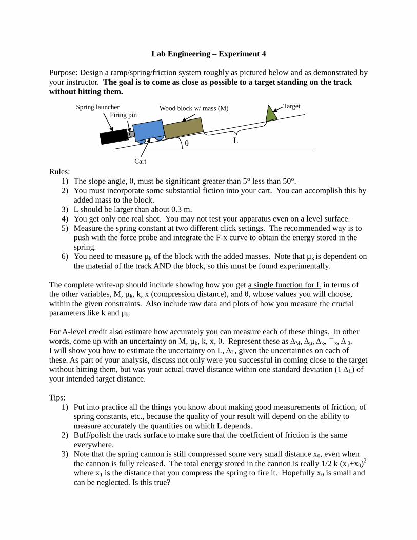
Purpose: Design a ramp/spring/friction system roughly as pictured below and as demonstrated by
your instructor. The goal is to come as close as possible to a target standing on the track
without hitting them.
Rules:
1) The slope angle, , must be significant greater than 5° less than 50°.
2) You must incorporate some substantial fiction into your cart. You can accomplish this by
added mass to the block.
3) L should be larger than about 0.3 m.
4) You get only one real shot. You may not test your apparatus even on a level surface.
5) Measure the spring constant at two different click settings. The recommended way is to
push with the force probe and integrate the F-x curve to obtain the energy stored in the
spring.
6) You need to measure µk of the block with the added masses. Note that µk is dependent on
the material of the track AND the block, so this must be found experimentally.
The complete write-up should include showing how you get a single function for L in terms of
the other variables, M, µk, k, x (compression distance), and , whose values you will choose,
within the given constraints. Also include raw data and plots of how you measure the crucial
parameters like k and µk.
For A-level credit also estimate how accurately you can measure each of these things. In other
words, come up with an uncertainty on M, µk, k, x, . Represent these as ΔM, Δµ, Δk x, Δ .
I will show you how to estimate the uncertainty on L, ΔL, given the uncertainties on each of
these. As part of your analysis, discuss not only were you successful in coming close to the target
without hitting them, but was your actual travel distance within one standard deviation (1 ΔL) of
your intended target distance.
Tips:
1) Put into practice all the things you know about making good measurements of friction, of
spring constants, etc., because the quality of your result will depend on the ability to
measure accurately the quantities on which L depends.
2) Buff/polish the track surface to make sure that the coefficient of friction is the same
everywhere.
3) Note that the spring cannon is still compressed some very small distance x0, even when
the cannon is fully released. The total energy stored in the cannon is really 1/2 k (x1+x0)2
where x1 is the distance that you compress the spring to fire it. Hopefully x0 is small and
can be neglected. Is this true?
θ
Wood block w/ mass (M) Spring launcher
Firing pin
Cart
Target
L
4) You must add mass to the block to obtain sufficiently high frictional values.
Complete a report on this experiment, giving details of your preparations, your calculation, and
your results, along with what you learned and how you later modified your apparatus or
calculation to ultimately make it work the way you intended. Once you have set up your
spring/cart/block/target system you should take before and after photos of the experiment to
make measuring travel distance easier.
Equipment:
Spring cannon, 2m track, wheeled cart with masses to add, wood block, meter stick, firing pins
for the cannon, target object, bricks to elevate one end of the track, force probe.
Please turn in the rubric at the beginning of the manual with your report.
To use the force probe:
- Connect the force probe to the lab laptop.
- Open Logger Pro.
- Set the force probe to ±50 N
- Click “* Force =” in Logger Pro above the data table.
- Click the force meter.
- Click “Zero”
- The spring launcher at one and two clicks is less than 50 N. At three clicks most are
above 50 N, so the reading with the force probe cannot be trusted.
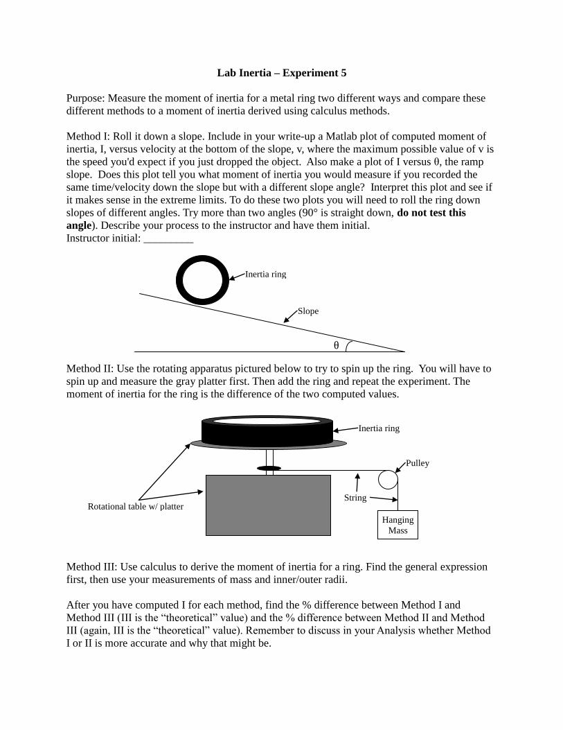
Lab Inertia – Experiment 5
Purpose: Measure the moment of inertia for a metal ring two different ways and compare these
different methods to a moment of inertia derived using calculus methods.
Method I: Roll it down a slope. Include in your write-up a Matlab plot of computed moment of
inertia, I, versus velocity at the bottom of the slope, v, where the maximum possible value of v is
the speed you'd expect if you just dropped the object. Also make a plot of I versus , the ramp
slope. Does this plot tell you what moment of inertia you would measure if you recorded the
same time/velocity down the slope but with a different slope angle? Interpret this plot and see if
it makes sense in the extreme limits. To do these two plots you will need to roll the ring down
slopes of different angles. Try more than two angles (90° is straight down, do not test this
angle). Describe your process to the instructor and have them initial.
Instructor initial: _________
Method II: Use the rotating apparatus pictured below to try to spin up the ring. You will have to
spin up and measure the gray platter first. Then add the ring and repeat the experiment. The
moment of inertia for the ring is the difference of the two computed values.
Method III: Use calculus to derive the moment of inertia for a ring. Find the general expression
first, then use your measurements of mass and inner/outer radii.
After you have computed I for each method, find the % difference between Method I and
Method III (III is the “theoretical” value) and the difference between Method II and Method
III (again, III is the “theoretical” value). Remember to discuss in your Analysis whether Method
I or II is more accurate and why that might be.
Hanging
Mass
Inertia ring
Pulley
Rotational table w/ platter String
θ
Inertia ring
Slope

Write up the report in the standard style describing your experiments. Note that two different
setups require two different diagrams in the Methods section. Include the calculus derivation of
your expression for moment of inertia. For Methods I/II decide which variable is known LEAST
accurately, that is, which one is responsible for creating the largest error in your result?
Equipment:
Large metal ring, rotational table, standard masses, pulleys, wood plank (slope), bricks to set
slope angle, vernier calipers, meter stick, string, rotational platter, stop watch.
Please turn in the rubric at the beginning of the manual with your report.
Lab Raft – Experiment 6
Construct a raft from the specified materials to hold a number of pennies that you will predict.
The winning team must hold the most pennies and ALSO correctly predict the number of pennies
it will hold, within the errors.
In your report, give your single equation for N, the number of pennies that the raft will support
without sinking. This equation will be in terms of any other important measurable variables. Be
sure to measure EVERYTHING (don't assume!)
Also, estimate uncertainties on each of the other parameters in your equation and compute an
uncertainty on the number of pennies the raft will hold, ΔN, using the same method as Lab 4. For
example, you don't know the boat volume with infinite precision...so let ΔV be the uncertainty on
the volume of your boat in cm3. Do you claim to know the volume of your boat to ΔV =1 cm
3,
ΔV = 0.5 cm3, ΔV = 0.1 cm
3? How about the mass of a penny; do you know that to ΔM =1 g or
better? In other words, estimate the level of uncertainty on your ability to measure the key
variables you need to measure to predict N.
Equipment:
A big vat of some liquid, balsa wood sheets for each group, knife, hot glue, lots of pennies
Please turn in the rubric at the beginning of the manual with your report.