phyluce DocumentationRelease 2.0.0

Brant C. Faircloth

December 31, 2013

Contents

1 Guide 31.1 Purpose . . . . . . . . . . . . . . . . . . . . . . . . . . . . . . . . . . . . . . . . . . . . . . . . . . 31.2 Installation . . . . . . . . . . . . . . . . . . . . . . . . . . . . . . . . . . . . . . . . . . . . . . . . 41.3 Configuration . . . . . . . . . . . . . . . . . . . . . . . . . . . . . . . . . . . . . . . . . . . . . . . 101.4 Data Pre-processing . . . . . . . . . . . . . . . . . . . . . . . . . . . . . . . . . . . . . . . . . . . 101.5 Read Assembly . . . . . . . . . . . . . . . . . . . . . . . . . . . . . . . . . . . . . . . . . . . . . . 131.6 UCE Processing for Phylogenomics . . . . . . . . . . . . . . . . . . . . . . . . . . . . . . . . . . . 15

2 Project info 292.1 Citing . . . . . . . . . . . . . . . . . . . . . . . . . . . . . . . . . . . . . . . . . . . . . . . . . . . 292.2 License . . . . . . . . . . . . . . . . . . . . . . . . . . . . . . . . . . . . . . . . . . . . . . . . . . 292.3 Changelog . . . . . . . . . . . . . . . . . . . . . . . . . . . . . . . . . . . . . . . . . . . . . . . . 302.4 Attributions . . . . . . . . . . . . . . . . . . . . . . . . . . . . . . . . . . . . . . . . . . . . . . . . 302.5 Funding . . . . . . . . . . . . . . . . . . . . . . . . . . . . . . . . . . . . . . . . . . . . . . . . . . 312.6 Acknowledgements . . . . . . . . . . . . . . . . . . . . . . . . . . . . . . . . . . . . . . . . . . . 32

Bibliography 33

i

ii

phyluce Documentation, Release 2.0.0

Release v2.0.0. (Changelog)

Author Brant Faircloth

Date 31 December 2013 19:06 CST (-0600)

Copyright This documentation is available under a Creative Commons (CC-BY) license.

phyluce (phy-loo-chee) is a software package that was initially developed for analyzing data collected from ultracon-served elements in organismal genomes (see References and http://ultraconserved.org for additional information).

The package now includes a number of tools spanning:

• the assembly of raw read data to contigs

• the separation of UCE loci from assembled contigs

• parallel alignment generation, alignment trimming, and alignment data summary methods in preparation foranalysis

• alignment and SNP calling using UCE or other types of raw-read data.

As it stands, the phyluce package is useful for analyzing both data collected from UCE loci and also data collectionfrom other types of loci for phylogenomic studies at the species, population, and individual levels.

phyluce is open-source (see License) and we welcome contributions from anyone who is interested. Please make apull request on github. The issue tracker for phyluce is also available on github. If you have an issue, please do all thatyou can to provide sufficient data and a test case demonstrating the issue.

Contents 1

phyluce Documentation, Release 2.0.0

2 Contents

CHAPTER 1

Guide

1.1 Purpose

Phylogenomics offers the possibility of helping to resolve the Tree of Life. To do this, we often need either verycheap sources of organismal genome data or decent methods of subsetting larger genomes (e.g., vertebrates; 1 Gbp)such that we can collect data from across the genome in an efficient and economical fashion, find the regions of eachgenome that are shared among organisms, and attempt to infer the evolutionary history of the organisms in whichwe’re interested using the data we collect.

Genome reduction techniques offer one way to collect these types of data from both small- and large-genome or-ganisms. These “reduction” techniques include various flavors of amplicon sequencing, RAD-seq (Restriction siteAssociated DNA markers), RNA-seq (transcriptome sequencing), and sequence capture methods.

phyluce is a software package for working with data generated from sequence capture of UCE (ultra-conservedelement) loci, as first published in [BCF2012]. Specifically, phyluce is a suite of programs to:

• assemble raw sequence reads from Illumina platforms into contigs

• determine which contigs represent UCE loci

• filter potentially paralagous UCE loci

• generate different sets of UCE loci across taxa of interest

Additionally, phyluce is capable of the following tasks, which are generally suited to any number of phylogenomicanalyses:

• produce large-scale alignments of these loci in parallel

• manipulate alignment data prior to further analysis

• convert alignment data between formats

• compute statistics on alignments and other data

phyluce is written to process data/individuals/samples/species in parallel, where possible, to speed execution. Par-allelism is achieved through the use of the Python multiprocessing module, and most computations are suited toworkstation-class machines or servers (i.e., rather than clusters). Where cluster-based analyses are needed, phylucewill produce the necessary outputs for input to the cluster/program that you are running so that you can setup the runaccording to your cluster design, job scheduling system, etc. Clusters are simply too heterogenous to do a good job atthis part of the analytical workflow.

3

phyluce Documentation, Release 2.0.0

1.1.1 Short-term goals (cli branch, v2.0.0+)

We are currently working on a new release (this documentation) to:

• ease the burden of installing dependencies using conda

• simplify the CLI (command-line interface) of phyluce

• standardize HOW you run various analyses

• improve test coverage of the code by unittests

• improve and standardize the documentation

1.1.2 Longer-term goals (v2.0.x and beyond)

We are also working towards adding:

• SNP-calling pipelines (sensu [BTS2013])

• sequence capture bait design

• identification of UCE loci

Much of this code is already written and in use by several of the Developed the UCE approach. As we test and improvethese functions, we will add them to the code in the future.

1.1.3 Who wrote this?

This documentation was written primarily by Brant Faircloth (http://faircloth-lab.org). Brant is also responsible forthe development of most of the phyluce code. Faults within the code are his.

You can find additional authors and contributors in the Authors and Developed the UCE approach sections.

1.2 Installation

phyluce uses a number of tools that allow it to assemble data, search for UCE loci, align results reads, manipulatealignments, prepare alignments for analysis, etc. To accomplish these goals, phyluce uses wrappers around a numberof programs that do each of these tasks (sometimes phyluce can use several different programs that accomplish thesame task in different ways). As a result, the dependency chain , or the programs that phyluce requires to run, isreasonably complex.

In previous versions (< 2.x), we required users to install a number of different software packages, get those into theuser’s $PATH, cross their fingers, and hope that everything ran smoothly (it usually did not).

In the current versions (> 2.x), we have removed a number of dependencies, and we very strongly suggest that usersinstall phyluce using either the anaconda or miniconda Python distributions.

Note: We do not support installing phyluce through means other than the conda installer. This means that we do nottest phyluce against any binaries, other than those we build and distribute through conda. However, with this in mind,you can configure phyluce to use binaries of different provenance using options in the Configuration section.

4 Chapter 1. Guide

phyluce Documentation, Release 2.0.0

1.2.1 Why conda?

It may seem odd to impose a particular disitribution on users, and we largely agree. However, conda makes it veryeasy for us to distribute both Python and non-Python packages (e.g. velvet, abYss, etc.), setup identical environmentsacross very heterogenous platforms (unices, osx, etc.), make sure all the $PATHs are correct, and have things runlargely as expected. Using conda has several other benefits, including environment separation similar to virtualenv. Inshort, using conda gets us as close to a “one-click” install that we will probably ever get.

1.2.2 Install Process

Important: We build and test phyluce using 64-bit, linux and osx computers (i.e., x86_64). Most modern computersare of this type. As such, we only support phyluce on 64-bit (x86_64) machines, and the conda packges that we havebuilt are only available for this architecture. We can potentially add x86 support if it is a major request.

Important: We do not support phyluce on Windows.

The installation process is now a 3-step process. You need to:

1. Install JAVA

2. Install conda (either anaconda or miniconda)

3. Install phyluce

Installing phyluce will install all of the required binaries, libraries, and Python dependencies.

Install JAVA

Although we’re using conda, you need to install a JAVA distribution for your platform. You should install JAVA7, asthat will ensure a number of future tools in phyluce will work on your platform. Installing JAVA is a little tricky acrossdifferent platforms (and somewhat beyond the scope of this document), but we described, below, how we usually doit.

If you do not see your (linux) distribution, check your package manager.

Apple OS X

To install JAVA 1.7, download and install the JAVA 1.7 package from Oracle here:http://www.java.com/en/download/manual.jsp

CentOS/Fedora linux

You can install the JRE with the following yum command:

su -c "yum install java-1.7.0-openjdk"

Debian/Ubuntu linux

You can install the JRE with the following apt-get command:

1.2. Installation 5

phyluce Documentation, Release 2.0.0

sudo apt-get install openjdk-7-jre

Install Anaconda or miniconda

After you installed JAVA, you need to install anaconda or miniconda. Which one you choose is up to you, your needs,how much disk space you have, and if you are on a fast/slow connection.

Tip: Do I want anaconda or miniconda? The major difference between the two python distributions is that anacondacomes with many, many packages pre-installed, while miniconda comes with almost zero packages pre-installed. Assuch, the anaconda distribution is roughly 200-500 MB in size while the miniconda distribution is 15-30 MB in size.

anaconda

Follow the instructions here for your platform: http://docs.continuum.io/anaconda/install.html

miniconda

Find the correct miniconda-2.x.x file for your platform from http://repo.continuum.io/miniconda/ and download thatfile. When that has completed, run:

bash Miniconda-2.2.x-Linux-x86_64.sh [linux]bash Miniconda-2.2.x-MacOSX-x86_64.sh [osx]

Now, you need to edit your $PATH to add the Miniconda distribution. You can do that manually using a text editor(the best way), or you can quickly quickly run:

echo "export PATH=$HOME/anaconda/bin:\${PATH}" >> ~/.bashrc [if you use BASH]echo "export PATH=$HOME/anaconda/bin:\${PATH}" >> ~/.zshrc [if you use ZSH]

Note: Once you have installed Miniconda, it is called anaconda forevermore.

Checking your $PATH

Regardless of how you install anaconda, you need to check that you’ve installed the package correctly. To ensure thatthe correct location for conda or miniconda are added to your $PATH (this occurs automatically on the $BASH shell),you can try the following, which should show the path to the anaconda distribution:

$ echo $PATH | grep anaconda | awk ’{split($0,a,":"); print a[1]}’/Users/bcf/anaconda/bin

You can also check that you have installed anaconda correctly by running the python -V command:

$ python -VPython 2.7.6 :: Anaconda 1.8.0 (x86_64)

Notice that the output shows we’re using the “Anaconda 1.8.0” version of Python. If you do not see the expectedoutput, then you likely need to edit your $PATH variable to add anaconda or miniconda as the first entry.

Should you need to edit your path, the easiest way to do that is to open ~/.bashrc with a text editor (if you areusing ZSH, this will be ~/.zshrc) and add, as the last line:

6 Chapter 1. Guide

phyluce Documentation, Release 2.0.0

export PATH=$HOME/path/to/conda/bin:$PATH

where $HOME/path/to/conda/bin is the location of anaconda/miniconda in your home directory (usually$HOME/anaconda/bin or $HOME/miniconda/bin).

Add the faircloth-lab repository to conda

You need to add the location of the packages we need to your conda distributions. to do taht, you have to add thefaircloth-lab conda repository to conda. You can do that with the following command, which automatically edits your~/.condarc file):

conda config --add channels http://conda.binstar.org/faircloth-lab

Install phyluce

Now, installing phyluce and all of it’s dependencies is simply a matter of running:

conda install phyluce

This step will also automatically configure phyluce to know where all of the different binaries are located (the subjectof the Configuration section).

Run phyluce

Once you’ve installed phyluce using conda, there will be an executable file named phyluce in your $PATH that we willrun for all subsequent analyses. You can find the location of the executable using:

$ which phyluce/Users/bcf/anaconda/bin/phyluce

Because phyluce is in our $PATH, running phyluce should produce the following output:

$ phyluceusage: phyluce [-h] [-V] command ...

phyluce is a software package for processing UCEand other phylogenomic datafor systematics andpopulation genetics.

positional arguments:commandassemble Assemble cleaned/trimmed sequencing reads.fetch Fetch (AKA get) UCE contigs from assembled data.align Alignment routines for UCE (and other) FASTA data.convert Convert files to different formats.misc Miscellaneous utilities for files and directories.help Get help info on a phyluce command.

optional arguments:-h, --help show this help message and exit-V, --version show program’s version number and exit

1.2. Installation 7

phyluce Documentation, Release 2.0.0

1.2.3 What conda installs

When you install phyluce, it specifies a number of dependencies that it needs to run. conda is great because it will pullspecific versions of the required programs from the faircloth-lab conda repository and install those on your machine,setup the paths, etc.

Below is a list of what phyluce requires for installation.

3rd-party dependencies

• trimmomatic 0.32

• velvet 1.2.10

• abyss 1.3.7 (built with boost and google-sparsehash)

• lastz 1.02.00

• mafft 7.13

• muscle 3.8.31

• raxml 8.0.1

Python packages

• Python 2.7 (sets conda default Python to 2.7)

• numpy 1.7

• BioPython 1.62

• dendropy 3.12.0

• illumiprocessor 2.0.3

• phyluce 2.0.x

1.2.4 Added benefits

An added benefit of using conda and installing packages in this way is that you can also run all of these binarieswithout worrying about setting the correct $PATH, etc.

phyluce required MUSCLE for installation, and MUSCLE was installed by conda as a dependency of phyluce. Be-cause $HOME/anaconda/bin is part of our path now, and because phyluce installed MUSCLE, we can also justrun MUSCLE on the command-line, with:

$ muscle

MUSCLE v3.8.31 by Robert C. Edgar

http://www.drive5.com/muscleThis software is donated to the public domain.Please cite: Edgar, R.C. Nucleic Acids Res 32(5), 1792-97.

Basic usage

muscle -in <inputfile> -out <outputfile>

8 Chapter 1. Guide

phyluce Documentation, Release 2.0.0

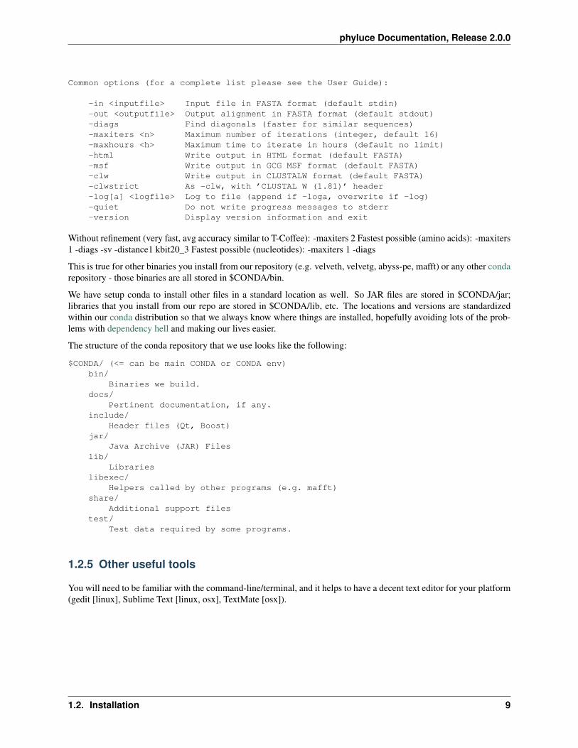
Common options (for a complete list please see the User Guide):

-in <inputfile> Input file in FASTA format (default stdin)-out <outputfile> Output alignment in FASTA format (default stdout)-diags Find diagonals (faster for similar sequences)-maxiters <n> Maximum number of iterations (integer, default 16)-maxhours <h> Maximum time to iterate in hours (default no limit)-html Write output in HTML format (default FASTA)-msf Write output in GCG MSF format (default FASTA)-clw Write output in CLUSTALW format (default FASTA)-clwstrict As -clw, with ’CLUSTAL W (1.81)’ header-log[a] <logfile> Log to file (append if -loga, overwrite if -log)-quiet Do not write progress messages to stderr-version Display version information and exit

Without refinement (very fast, avg accuracy similar to T-Coffee): -maxiters 2 Fastest possible (amino acids): -maxiters1 -diags -sv -distance1 kbit20_3 Fastest possible (nucleotides): -maxiters 1 -diags

This is true for other binaries you install from our repository (e.g. velveth, velvetg, abyss-pe, mafft) or any other condarepository - those binaries are all stored in $CONDA/bin.

We have setup conda to install other files in a standard location as well. So JAR files are stored in $CONDA/jar;libraries that you install from our repo are stored in $CONDA/lib, etc. The locations and versions are standardizedwithin our conda distribution so that we always know where things are installed, hopefully avoiding lots of the prob-lems with dependency hell and making our lives easier.

The structure of the conda repository that we use looks like the following:

$CONDA/ (<= can be main CONDA or CONDA env)bin/

Binaries we build.docs/

Pertinent documentation, if any.include/

Header files (Qt, Boost)jar/

Java Archive (JAR) Fileslib/

Librarieslibexec/

Helpers called by other programs (e.g. mafft)share/

Additional support filestest/

Test data required by some programs.

1.2.5 Other useful tools

You will need to be familiar with the command-line/terminal, and it helps to have a decent text editor for your platform(gedit [linux], Sublime Text [linux, osx], TextMate [osx]).

1.2. Installation 9

phyluce Documentation, Release 2.0.0

1.3 Configuration

Attention: If you installed phyluce using conda, the following section is unecessary for running your first dataanalysis.

phyluce is configured using the same system that conda uses to setup and maintain is .condarc file. Specifically, youuse the phyluce config option to update a YAML-formatted file at ~/.condarc. Although we provide the phyluce configoption as a helper, you can also edit this file by hand, provided that you maintain correct YAML structure.

1.4 Data Pre-processing

1.4.1 Demultiplexing

Because we are reducing genomes, and beceause we generally reduce genomes to a fraction of their original size,we can combine DNA libraries from many sources into a single lane of HiSeq (or even MiSeq) sequencing. And,because we are multiplexing these libraries prior to sequencing, we need to “demultiplex” these libraries after they’resequenced.

Demultiplexing is a tricky process, made trickier by the platform with which you are working. Thankfully, demulti-plexing (or “demuxing”) Illumina reads is rather simple. There are several options:

• Casava (the Illumina pipeline)

• fastx-toolkit

• bartab

I have also written splitaake_, which is a program to help demultiplex Illumina reads. splitaake_ is particularly usefulwhen you have very many sequence tags (aka “barcodes”) to demultiplex, when your sequence tags are long, or somecombination of the two.

To demultiplex your data with splitaake_, please see the website.

1.4.2 Read Counts

After demultiplexing, it’s always good to get an idea of the split of reads among your samples. This does two things:

1. Allows you to determine how well you split the run among your tags

2. Shows you which samples may be suboptimal (have very few reads)

Really unequal read counts mean that you may want to switch up your library quantification process (or your poolingsteps, prior to enrichment). Suboptimal read counts for particular libraries may or may not mean that the enrichmentsof those samples “failed”, but it’s generally a reasonable indication.

Because we’re working with fastq files, it’s reasonably easy to get read counts across all of the libraries (with a littledivision). Fastq files contains 4 lines for each read, so we need to get the count of all lines in each file and divide thoseresults by 4.

Assuming that your reads are in a directory structure like:

some-directory-name/bfidt-000_R1.fastq.gzbfidt-000_R2.fastq.gzbfidt-001_R1.fastq.gzbfidt-001_R2.fastq.gz

10 Chapter 1. Guide

phyluce Documentation, Release 2.0.0

you can count lines across all files in all directories, with:

for i in some-directory-name/*_R1.fastq.gz; do echo $i; gunzip -c $i | wc -l; done

This will output a list of results like:

bfidt-000_R1.fastq.gz10000000

bfidt-000_R2.fastq.gz16000000

If you divide these numbers by 4, then that is the count of R1 reads (the count of R2 reads should be equal).

1.4.3 Adapter- and quality- trimming

After you demultiplex your data, you generally end up with a number of files in a directory that look like the following.Specifically, if you used splitaake_:

some-directory-name/bfidt-000_R1.fastq.gzbfidt-000_R2.fastq.gzbfidt-001_R1.fastq.gzbfidt-001_R2.fastq.gz

or, if you used Casava:

Project_name/Sample_BFIDT-000

BFIDT-000_AGTATAGCGC_L001_R1_001.fastq.gzBFIDT-000_AGTATAGCGC_L001_R2_001.fastq.gz

Sample_BFIDT-001BFIDT-001_TTGTTGGCGG_L001_R1_001.fastq.gzBFIDT-001_TTGTTGGCGG_L001_R2_001.fastq.gz

Now, what you want to do is to clean these reads of adapter contamination and trim low-quality bases from all reads(and probably also drop reads containing “N” (ambiguous) bases. Then you want to interleave the resulting data,where read pairs are maintained, and also have an output file of singleton data, where read pairs are not.

You can do this however you like. For the steps that follow, you want a resulting directory structure that looks like(replace genus_species with your taxon names):

genus_species1/interleaved-adapter-quality-trimmed/

genus_species1-READ1and2-interleaved.fastq.gzgenus_species1-READ-singleton.fastq.gz

genus_species2/interleaved-adapter-quality-trimmed/

genus_species2-READ1and2-interleaved.fastq.gzgenus_species2-READ-singleton.fastq.gz

The “READ1and2” file should be in interleaved file containig both reads kept, and the READ file should contain thosedata where one read of the pair are kept (AKA singleton reads).

Read QC with illumiprocessor

I created a program that I use for adapter and quality trimming named illumiprocessor. It generally automates theseprocesses and produces output if the format we want downstream.

1.4. Data Pre-processing 11

phyluce Documentation, Release 2.0.0

If you used Casava, it will be easiest to place all of the demuliplexed reads into a single directory. If you used‘splitaake‘_, then things should be all set.

You need to generate a configuration file your-illumiprocessor.conf, that gives details of your reads, how you wantthem processed, and what renaming options to use. This file is an extension of the INI file used for ‘splitaake‘_ and itlooks like this:

[adapters]truseq1:AGATCGGAAGAGCACACGTCTGAACTCCAGTCAC*ATCTCGTATGCCGTCTTCTGCTTGAAAAAtruseq2:AGATCGGAAGAGCGTCGTGTAGGGAAAGAGTGTAGATCTCGGTGGTCGCCGTATCATTAAAAA

[indexes]bfidt-000:AACCGAGTTAbfidt-001:AATACTTCCGbfidt-002:AATTAAGGCCbfidt-003:AAGCTTATCC

[params]separate reads:Trueread1:{name}_R1.fastq.gzread2:{name}_R2.fastq.gz

[combos]genus_species1:bfidt-000genus_species2:bfidt-001genus_species3:bfidt-002genus_species4:bfidt-003

[remap]bfidt-000:genus_species1bfidt-001:genus_species2bfidt-002:genus_species3bfidt-003:genus_species4

This gives the adapter sequences to trim (with the index indicated by an asterisk) in [adapters], the indexes we used[indexes], whether reads are separate and a name-formatting convention [params], a mapping of species names toindex [combos], and a mapping of index names to species [remap].

You can run illumiprocessor against your data (in demultiplexed) with the following. If you do not have a multicoremachine, you may with to run with –cores=1. Additionally, multicore operations require a fair amount of RAM, so ifyou’re low on RAM, run with fewer cores:

mkdir uce-cleanpython ~/git/illumiprocessor/illumiprocessor.py \

demultiplexed \uce-clean \your-illumiprocesser.conf \--remap \--clean \--cores 12 \--complex

The clean data will appear in uce-clean with the following structure:

uce-clean/genus_species1/

interleaved-adapter-quality-trimmed/genus_species-READ1and2-interleaved.fastq.gzgenus_species-READ-singleton.fastq.gz

stats/

12 Chapter 1. Guide

phyluce Documentation, Release 2.0.0

genus_species-READ1.fastq.gz-adapter-contam.txtgenus_species--READ2.fastq.gz-adapter-contam.txtsickle-trim.txt

untrimmed/genus_species-READ1.fastq.gz (symlink)genus_species-READ1.fastq.gz (symlink)

genus_species2/interleaved-adapter-quality-trimmed/

genus_species-READ1and2-interleaved.fastq.gzgenus_species-READ-singleton.fastq.gz

stats/genus_species-READ1.fastq.gz-adapter-contam.txtgenus_species--READ2.fastq.gz-adapter-contam.txtsickle-trim.txt

untrimmed/genus_species-READ1.fastq.gz (symlink)genus_species-READ1.fastq.gz (symlink)

interleaved-adapter-quality-trimmed contains the cleaned read data in interleaved format, with one file containing“READ1and2” (both reads kept) and another file containing “READ” data, where singleton reads are kept (singletonssometimes result from the QC routines).

1.5 Read Assembly

Once your reads are clean, you’re ready to assemble. At the moment, we use velvet and VelvetOptimiser for assembly,although I’m considering adding similar routines for ABySS.

Most of this process is automated using code within phyluce. But, before you runt the automated routines, you needto get a good idea of the kmer ranges within which you will assembling, prior to starting the assembly process withthe automated code.

In the following, I assume your directory structure looks like this (which results from illumiprocessor):

uce-clean/genus_species1/

interleaved-adapter-quality-trimmed/genus_species-READ1and2-interleaved.fastq.gzgenus_species-READ-singleton.fastq.gz

1.5.1 Finding a reasonable kmer range

For the automated procedure, we need to have a reasonably good idea of the kmer range that we want to plug into theautomated process. After several rounds of this process, you generally get a good idea of what works. However, I stillempirically check this range against a couple of test assemblies before running many assemblies with the automationcode.

To determine this range, you want to assemble a test batch of reads using a range of kmer values. I usually do this for4-5 taxa in the data set I just cleaned using kmer values in the range of 63-75. Depending on the so-called “optimal”,kmer value reported by VelvetOptimiser, I’ll adjust the upper and lower limits of this range, hopefully settling on arange of values that will work across the remaining batches of reads during the automated process.

To assemble a test batch of reads, you want to run the following with VelvetOptimiser. The commands below assumesyou have an 8-core computer (-t 8) and a sizable amount of RAM (>= 24 GB). If you have fewer cores or less RAM,you’ll need to adjust the -t parameter. You probably want to initially try a range of kmer values between 63 and 75.

1.5. Read Assembly 13

phyluce Documentation, Release 2.0.0

So, pick a taxon to test with. You probably want to start with something having roughly the mean number of readsacross all taxa you included in a run.

First, you want to enter a particular taxons uce-clean directory of reads and create an assembly directory to hold theassembly results:

cd uce-clean/genus_species1/mkdir assemblycd assembly

Now that you’re in the directory, you want to run VelvetOptimiser against the interleaved read data that are onedirectory up:

VelvetOptimiser -s 63 -e 75 -t 8 -a -c ncon \-f ’-fastq.gz \-shortPaired ../interleaved-adapter-quality-trimmed/genus_species-READ1and2-interleaved.fastq.gz \-short ../interleaved-adapter-quality-trimmed/genus_species-READ-singleton.fastq.gz’

VelvetOptimiser will assemble the read data in the interleaved-adapter-quality-trimmed directory and when it is fin-ished, will output the optimal kmer size for the assembly to stdout. Write down and/or remember this number (probablybest to write it down).

You also want to ensure that the optimal kmer size is inside of the range that you passed to the program. If it is,conduct several additional assemblies with other data to ensure that this range works well across all of your samples.

If the “optimal” kmer size is at the edge of the range you input, then you should adjust the range of kmer values to try,and re-assemble the data to see if the next “optimal” kmer value is within the range you input.

Once you have a good idea of the range size for the data, you may wish to delete the test assembly directories. Youcan also keep them, but you will need to manually symlink over the contigs folder (see below).

1.5.2 Running assemblo.py

Once you have a good idea of the range that will work for your data, you can run the automated script to assembleyour data:

python ~/git/phyluce/bin/assembly/assemblo.py uce-clean 63 75 7

This will run VelvetOptimiser across your data in the uce-clean directory, using a range of kmer values from 63-75and 7 compute cores. As before, you may need to adjust the number of compute cores for your system and/or amountof RAM.

assemblo.py will output the results of each assembly to stdout, giving the file name, optimal kmer size, resulting n50,and an indication of whether the optimal kmer size was reached during assembly.

If the optimal kmer size is not reached during assembly, you may wish to re-assembly problematic contigs by handwith different parameters (a smaller or larger range).

If you want to exclude certain directories nested within uce-clean, for instance, you can run:

python ~/git/phyluce/bin/assembly/assemblo.py uce-clean 63 75 7 \--exclude genus_species1 genus_species2

Within the uce-clean directory, assemblo.py will create a directory named contigs that contain symlinks to the resultingassembly data for each taxon.

If you assembled any data by hand that are in assembly directories, you will also want to symlink those results in thecontigs directory.

14 Chapter 1. Guide

phyluce Documentation, Release 2.0.0

1.5.3 Linking contig assemblies into the contigs directory

assemblo.py will assemble your contigs, and symlink them into a contigs directory. These symlinks allow you toreasonably keep track of which assembly is linked to a particular taxon, maintaining continuity in your data.

If you have manually assembled any contigs outside of assembly, you will also need to manually link those into thecontigs folder with something like:

ln -s uce-clean/genus_species1/genus_species1/assembly/auto_data_75/contigs.fa \contigs/genus_species1.contigs.fasta

The other downside of symlinks is that they tend not to “travel” very well. Meaning, if you want to move the contigsfolder somewhere else, this will often break the symlinks created by assemblo.py. This is often painful to fix by hand,so there’s a bit of code in phyluce_ to help you do that. If you have reads in:

/path/to/my/uce-clean/contigs

and you want to create a new contigs folder elsewhere, you want to replace the path in the original symlink with thepath in the new symlink. So, you can run:

python ~/Git/brant/phyluce/bin/share/replace_many_links.py \/path/to/my/uce-clean/contigs \/path/to/my/uce-clean/clean/ \/new/path/to/my/uce-clean/location/name-of-new-folder

1.5.4 Determining success or failure of an assembly/enrichment

This is a little bit tricky without having some previous experience. Generally speaking, if you cannot reasonably easilyfind an optimal kmer value for a given assembly (the “optimal” kmer is always at the top or bottom of the range), thenthe assembly (and data) are likely not as good as they should be. The causes of this are too many to describe here, butinclude low-coverage, poor enrichment, bad libraries, contamination, etc.

You should generally see that the total number of contigs assembled is within 1-3X the number of contigs that youtargeted with your enrichment probe set. Ideally, you also want the assembled contigs to have an n50 > 300-400 bp.You typically do not want to see only very large (>10 Kbp) contigs assembled or only very small (< 300 bp) contigsassembled.

Again, these results depend on a variety of factors including starting DNA quality, library size, the efficiency of theenrichment, the number of post-enrichment PCR cycles you used, the amount of sequence data collected for a givenlibrary, etc., etc., etc.

1.6 UCE Processing for Phylogenomics

The workflow described below is meant to outline the process needed for analyzing UCE in phylogenetic contexts -meaning that you are interested in addressing questions at the species level or deeper.

1.6.1 Probe sets

Depending on the taxa you are targeting and the probe set that you are using, you will need to adjust the probe set nameto reference the fasta file of those probes you used. Below, I have used the uce-5k-probes.fasta probe set. However,the probe set that use could be one of:

1. uce-2k-probes.fasta (tetrapods/birds/mammals)

1.6. UCE Processing for Phylogenomics 15

phyluce Documentation, Release 2.0.0

2. uce-5k-probes.fasta (tetrapods/birds/mammals)

1.6.2 Outgroup data and probe set downloads

We have started to standardize and provide prepared sets of UCE probes and outgroup data. The outgroup data aresliced from available genome sequences, and the probe sets and outgroup data are version controlled for a particularset of taxa (e.g., tetrapods, fish). If you would like to use these in your own analyses, to extend your current data setor to provide an outgroup, you can download them from uce-probe-sets

1.6.3 Indentifying contigs matching UCE loci

After assembly, we have generated contigs from raw reads. These contigs reside in the contigs resulting from assembly.During the next part of the process, we need to determine which of the assembled contigs match UCE loci and whichdo not. We also need to remove any contigs that appear to be duplicates as a result of assembly/other problems or aduplication event(s).

The first thing to do is to make sure that our probe set does not contain any duplicates. So, you probably want to alignthe file of probe sequences to itself (if you’re using a probe-set from github, the this file should be included):

python phyluce/bin/share/easy_lastz.py \--target uce-5k-probes.fasta \--query uce-5k-probes.fasta \--identity 85 \--output uce-5k-probes.fasta.toself.lastz

Now, what we need to do is to align our probes to our contigs. First, you want to make a directory to hold our output:

mkdir /path/to/output/lastz

Now, we want to find which probes match which UCE loci. To do this, the code will also strip the probe numbers offof particular loci in the uce-5k-probes.fasta file (stripping off the probe numbers allows us to merge all probes downto a single locus). The default regular expression assumes your probes are named similarly to uce-NNN_pN. If that isnot the case, you will need to input a different regular expression to convert the probe names to locus names.

Note, too, that we’re passing the uce-5k-probes.fasta.toself.lastz to the code so that we can also exclude any UCE lociwhose probes happen to overlap themselves:

python phyluce/bin/assembly/match_contigs_to_probes.py \/path/to/velvet/assembly/contigs/ \/path/to/uce-5k-probes.fasta \/path/to/output/lastz \--dupefile uce-5k-probes.fasta.toself.lastz

When you run this code, you will see output similar to:

genus_species1: 1031 (70.14%) uniques of 1470 contigs, 0 dupe probe matches, 48 UCE probes matching multiple contigs, 117 contigs matching multiple UCE probesgenus_species2: 420 (68.52%) uniques of 613 contigs, 0 dupe probe matches, 30 UCE probes matching multiple contigs, 19 contigs matching multiple UCE probesgenus_species3: 1071 (63.15%) uniques of 1696 contigs, 0 dupe probe matches, 69 UCE probes matching multiple contigs, 101 contigs matching multiple UCE probes

Now, what this program does is to use lastz_ to align all probes to the contigs. It basically ignores those contigsthat don’t match probes (no matches) and screens the results to ensure that, of the matches, only one contig matchesprobes from one UCE locus and that only probes from one UCE locus match one contig. Everything outside of theseparameters is dropped.

The resulting files will be in the:

16 Chapter 1. Guide

phyluce Documentation, Release 2.0.0

/path/to/output/lastz

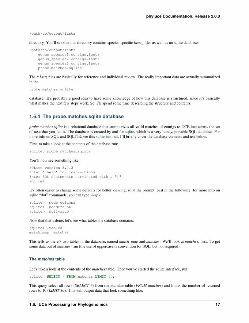
directory. You’ll see that this directory contains species-specific lastz_ files as well as an sqlite database:

/path/to/output/lastzgenus_species1.contigs.lastzgenus_species2.contigs.lastzgenus_species3.contigs.lastzprobe.matches.sqlite

The *.lastz files are basically for reference and individual review. The really important data are actually summarizedin the:

probe.matches.sqlite

database. It’s probably a good idea to have some knowledge of how this database is structured, since it’s basicallywhat makes the next few steps work. So, I’ll spend some time describing the structure and contents.

1.6.4 The probe.matches.sqlite database

probe.matches.sqlite is a relational database that summarizes all valid matches of contigs to UCE loci across the setof taxa that you fed it. The database is created by and for sqlite, which is a very handy, portable SQL database. Formore info on SQL and SQLITE, see this sqlite-tutorial. I’ll briefly cover the database contents and use below.

First, to take a look at the contents of the database run:

sqlite3 probe.matches.sqlite

You’ll now see something like:

SQLite version 3.7.3Enter ".help" for instructionsEnter SQL statements terminated with a ";"sqlite>

It’s often easier to change some defaults for better viewing, so at the prompt, past in the following (for more info onsqlite “dot” commands, you can type .help):

sqlite> .mode columnssqlite> .headers onsqlite> .nullvalue .

Now that that’s done, let’s see what tables the database contains:

sqlite> .tablesmatch_map matches

This tells us there’s two tables in the database, named match_map and matches. We’ll look at matches, first. To getsome data out of matches, run (the use of uppercase is convention for SQL, but not required):

The matches table

Let’s take a look at the contents of the matches table. Once you’ve started the sqlite interface, run:

sqlite> SELECT * FROM matches LIMIT 10;

This query select all rows (SELECT *) from the matches table (FROM matches) and limits the number of returnedrows to 10 (LIMIT 10). This will output data that look something like:

1.6. UCE Processing for Phylogenomics 17

phyluce Documentation, Release 2.0.0

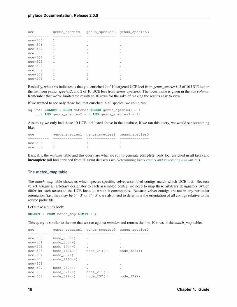
uce genus_species1 genus_species2 genus_species3---------- -------------- -------------- --------------uce-500 1 . .uce-501 1 . .uce-502 1 . .uce-503 1 1 1uce-504 1 . .uce-505 1 . .uce-506 . . .uce-507 1 . .uce-508 1 1 .uce-509 1 1 1

Basically, what this indicates is that you enriched 9 of 10 targeted UCE loci from genus_species1, 3 of 10 UCE loci inthe list from genus_species2, and 2 of 10 UCE loci from genus_species3. The locus name is given in the uce column.Remember that we’ve limited the results to 10 rows for the sake of making the results easy to view.

If we wanted to see only those loci that enriched in all species, we could run:

sqlite> SELECT * FROM matches WHERE genus_species1 = 1...> AND genus_species2 = 1 AND genus_species3 = 1;

Assuming we only had those 10 UCE loci listed above in the database, if we ran this query, we would see somethinglike:

uce genus_species1 genus_species2 genus_species3---------- -------------- -------------- --------------uce-503 1 1 1uce-509 1 1 1

Basically, the matches table and this query are what we run to generate complete (only loci enriched in all taxa) andincomplete (all loci enriched from all taxa) datasets (see Determining locus counts and generating a taxon-set).

The match_map table

The match_map table shows us which species-specific, velvet-assembled contigs match which UCE loci. Becausevelvet assigns an arbitrary designator to each assembled contig, we need to map these arbitrary designators (whichdiffer for each taxon) to the UCE locus to which it corresponds. Because velvet contigs are not in any particularorientation (i.e., they may be 5’ - 3’ or 3’ - 5’), we also need to determine the orientation of all contigs relative to thesource probe file.

Let’s take a quick look:

SELECT * FROM match_map LIMIT 10;

This query is similar to the one that we ran against matches and returns the first 10 rows of the match_map table:

uce genus_species1 genus_species2 genus_species3---------- -------------- -------------- --------------uce-500 node_233(+) . .uce-501 node_830(+) . .uce-502 node_144(-) . .uce-503 node_1676(+) node_243(+) node_322(+)uce-504 node_83(+) . .uce-505 node_1165(-) . .uce-506 . . .uce-507 node_967(+) . .uce-508 node_671(+) node_211(-) .uce-509 node_544(-) node_297(+) node_37(+)

18 Chapter 1. Guide

phyluce Documentation, Release 2.0.0

As stated above, these results show the “hits” of velvet-assembled contigs to particular UCE loci. So, if we wereto open the genus_species1.contigs.fasta symlink (which connects to the assembly) in the contigs folder, the contignamed node_233 corresponds to UCE locus uce-500.

Additionally, each entry in the rows also provides the orientation for particular contigs (-) or (+). This orientation isrelative to the orientation of the UCE probes/locus in the source genome (e.g., chicken for tetrapod probes).

We use this table to generate a FASTA file of UCE loci for alignment (see Determining locus counts and generating ataxon-set), after we’ve identified the loci we want in a particular data set. The code for this step also uses the associatedorientation data to ensure that all the sequence data have the same orientation prior to alignment (some aligners willforce alignment of all reads using the given orientation rather than also trying the reverse complement and picking thebetter alignment of the two).

1.6.5 Determining locus counts and generating a taxon-set

Now that we know the taxa for which we’ve enriched UCE loci and which contigs we’ve assembled match whichUCE loci, we’re ready to generate some data sets. The data set generation process is pretty flexible - you can selectwhich taxa you would like to group together for an analysis, you can generate complete and incomplete data matrices,and you can also include additional data from the provided outgroup files and data (see Outgroup data and probe setdownloads) or previous runs. We’ll start simple.

Complete matrix data set

First, we’ll generate a data set from only the current UCE enrichments, and it will be complete - meaning that we willnot include loci where certain taxa have no data (either the locus was not enriched for that taxon or removed duringthe filtering process for duplicate loci).

The first step of generating a data set is to identify those loci present in the taxa with which we’re working. First, youneed to create a configuration (text) file denoting the taxa we want in the data set. It should look like this:

[dataset1]genus_species1genus_species2genus_species3

Let’s assume you name this file datasets.conf. Now, you want to run the following against this file, along with severalother files we’ve created previously:

python phyluce/bin/assembly/get_match_counts.py \/path/to/output/lastz/probe.matches.sqlite \/path/to/your/datasets.conf \’dataset1’ \--output /path/to/some/output-file/dataset1.conf

This will basically run a query against the database, and pull out those loci for those taxa in the datasets.conf filehaving UCE contigs. The output will look something like:

Shared UCEs: 500

genus_species1:108genus_species2:93genus_species3:71

This means that 500 loci are shared amongst the 3 taxa in datasets.conf. We might have had more, but genus_species1caused us to drop 108 loci, genus_species2 caused us to drop 93 loci, and genus_species3 caused us to drop 71 loci.

1.6. UCE Processing for Phylogenomics 19

phyluce Documentation, Release 2.0.0

Now, you might think that increasing the locus count is simply a matter of removing genus_species1 from the list oftaxa. This is not strictly true, however, given the vagaries of hits and misses among taxa. get_match_counts.py hasseveral other options to help you determine which taxa may be causing problems, but picking the best combination oftaxa to give you the highest number of loci is a somewhat hard optimization problem.

If you want to generate/evalaute additional data sets with different taxa, you can simply append that list to thedatasets.conf file like so:

[dataset1]genus_species1genus_species2genus_species3

[dataset2]genus_species2genus_species3genus_species4genus_species5genus_species6

and then run get_match_counts.py against this new section:

python phyluce/bin/assembly/get_match_counts.py \/path/to/output/lastz/probe.matches.sqlite \/path/to/your/datasets.conf \’dataset2’ \--output /path/to/some/output-file/dataset2.conf

Incomplete data matrix

You may not always want a complete data matrix or generating a complete matrix drops too many loci for your tastes.That’s cool. You can generate an incomplete dataset like so:

python phyluce/bin/assembly/get_match_counts.py \/path/to/output/lastz/probe.matches.sqlite \/path/to/your/datasets.conf \’dataset1’ \--output /path/to/some/output-file/dataset1-incomplete.conf--incomplete-matrix

This will generate a dataset that includes any loci enriched across the taxa in the datasets.conf file. This will alsoinclude a file named dataset1-incomplete.notstrict that contains those loci enriched for each taxon. We’ll need that ina minute (see Extracting relevant FASTA data)

Incorporating outgroup/other data

You may want to include outgroup data from another source into your datasets. This can be from the pre-processedoutgroup data files (see Outgroup data and probe set downloads), but it doesn’t need to be these outgroup data. Theseadditional data can also be contigs previously assembled from a different set of taxa.

The first step of this process is to setup your datasets.conf slightly differently - by indicating these external data withasterisks:

[dataset3]genus_species1genus_species2genus_species3

20 Chapter 1. Guide

phyluce Documentation, Release 2.0.0

genus_species4*genus_species5*

Then, you need to pass get_match_counts.py the location of the probe.matches.sqlite database previously generated asdescribed in Indentifying contigs matching UCE loci or downloaded as part of Outgroup data and probe set downloads:

python phyluce/bin/assembly/get_match_counts.py \/path/to/output/lastz/probe.matches.sqlite \/path/to/your/datasets.conf \’dataset3’ \--extend /path/to/some/other/probe.matches.sqlite \--output /path/to/some/output-file/dataset3-with-external.conf

To keep all this extension from getting too terribly crazy, I’ve limited the ability to include external data to essentiallya single set. If you have lots of data from many different enrichments, you’ll need to generate a contigs foldercontaining all these various assemblies (or symlinks to them), then align the probes to these data (see Indentifyingcontigs matching UCE loci). Once you do that, you can extend your current data set with all of these other data.

1.6.6 Extracting relevant FASTA data

After selecting the set of loci in which you’re interested, you need to generate a FASTA file containing the reads fromeach species-specific contig that corresponds to a locus in the set. This is reasonable easy.

Complete data matrix

To generate a FASTA file, we’re passing several previously used paths and the name of the output file fromget_match_counts.py on the third line below (/path/to/some/output-file/dataset1.conf ):

python phyluce/bin/assembly/get_fastas_from_match_counts.py \/path/to/velvet/assembly/contigs/ \/path/to/output/lastz/probe.matches.sqlite \/path/to/some/output-file/dataset1.conf \--output /path/to/some/output.fasta

Incomplete data matrix

To generate a FASTA file, we’re passing several previously used paths plus the name of the output file fromget_match_counts.py on the fourth line AND the name of the *.notstrict file on the fifth line:

python phyluce/bin/assembly/get_fastas_from_match_counts.py \/path/to/velvet/assembly/contigs/ \/path/to/output/lastz/probe.matches.sqlite \/path/to/some/output-file/dataset1-incomplete.conf \--incomplete-matrix /path/to/some/output-file/dataset1-incomplete.notstrict--output /path/to/some/output.fasta

Incorporating outgroup/other data

Because we’re incorporating external data, we need to pass the name of the external database, as before, as well as thename of the external contigs directory:

1.6. UCE Processing for Phylogenomics 21

phyluce Documentation, Release 2.0.0

python phyluce/bin/assembly/get_fastas_from_match_counts.py \/path/to/velvet/assembly/contigs/ \/path/to/output/lastz/probe.matches.sqlite \/path/to/some/output-file/dataset3-with-external.conf \--extend-db /path/to/some/other/probe.matches.sqlite \--extend-dir /path/to/some/other/contigs/ \--output /path/to/some/output.fasta

1.6.7 Aligning and trimming FASTA data

With all of that out of the way, things get much easier to deal with. We basically need to align our data across loci,and we’re largely ready to go. The remaining operations we can run on the data are format-conversions, QC steps orany number of other fun things.

Aligning this much data is reasonably computationally intensive - so this alignment step goes fastest if you havea multicore machine. You also have several alignment options available, although I would suggest sticking withMAFFT.

First, make a folder for the alignment output:

mkdir /path/to/alignment/output

Complete data matrix

The second line is the fasta created above (see Extracting relevant FASTA data), the second line is the path to theoutput, the third line gives the number of taxa in the alignment, –aligner mafft determines the alignment program, and–cores 8 denoted the number of cores to use for this step:

python phyluce/bin/align/seqcap_align_2.py \/path/to/some/output.fasta \/path/to/alignment/output \3 \--aligner mafft \--cores 8

Incomplete data matrix

The only difference for an alignment of incomplete data is that we also pass the –notstrict flag, which tells the code toexpect that some loci will not have data for all taxa:

python phyluce/bin/align/seqcap_align_2.py \/path/to/some/output.fasta \/path/to/alignment/output \3 \--aligner mafft \--incomplete-matrix \--cores 8

After checking the resulting alignment QC (see Alignment quality control), you will generally need to add in missingdata designators for taxa missing from the alignment of a given locus. This will basically allow you to generateconcatenated data sets and it may reduce error messages from other programs about files having unequal numbers oftaxa. To do this, you need to run:

22 Chapter 1. Guide

phyluce Documentation, Release 2.0.0

python phyluce/bin/align/add_missing_data_designators.py \/path/to/alignment/output \/path/to/alignment/output-with-missing-data/ \/path/to/some/output-file/dataset3-with-external.conf \/path/to/some/output-file/dataset3-with-external.notstrict

Alignment trimming

The alignment code “trims” alignments by default. Basically, this means that it removes ragged 5’ and 3’ edges froma given alignment. However, you may not want to run the trimming and just deal with the raw alignments output bymafft/muscle/dialign. No problem, you run seqcap_align_2.py just as above, but you add the –notrim option:

python phyluce/bin/align/seqcap_align_2.py \/path/to/some/output.fasta \/path/to/alignment/output \3 \--aligner mafft \--cores 8 \--notrim

Saté alignment

There is also an option to run Saté alignments instead of the default code. For the moment, this code lives inmpi_sate.py and you can run it locally with something like:

python phyluce/bin/align/mpi_sate.py \/path/to/some/output.fasta \/path/to/alignment/output \3 \/path/to/sate \/path/to/sate.cfg \--parallelism multiprocessing \--cores 8

This code will also run on MPI enabled machines, but that is generally beyond the scope of this HOWTO.

Alignment trimming only

If you have untrimmed (ragged) alignments that you would like to trim with the phyluce trimming procedures, youcan also run that:

python phyluce/bin/align/get_trimmed_alignments_from_untrimmed.py \/path/to/alignment/input \/path/to/output/for/trimmed/data/ \--input-format nexus--output-format nexus \--multiprocessing

1.6.8 Alignment quality control

There are many ways to QC alignments. The best way is to do it visually, but that gets somewhat hard when you havethousands of loci. There are several programs in the phyluce package that help you QC alignments. You probablyalways want to run:

1.6. UCE Processing for Phylogenomics 23

phyluce Documentation, Release 2.0.0

python ~/git/phyluce/bin/align/get_align_summary_data.py \/path/to/alignment/output-renamed \--input-format nexus

This will output a number of stats that look somewhat like (these examle data are from an incomplete matrix):

uce-1071.nex is < 100 bp longuce-720.nex is < 100 bp long

Lengths-----Total length(aln) 256066Average length(aln) 318.49004975195 CI length(aln) 10.6004273805Minimum length(aln) 64Maximum length(aln) 933

Taxa-----Average(taxa) 11.52611940395 CI(taxa) 0.37345195065min(taxa) 3max(taxa) 21Count(taxa:# alns) {3: 77, 4: 44, 5: 38, 6: 35, 7: 36, 8: 33, 9: 47, 10: 35, 11: 31, 12: 34, 13: 50, 14: 62, 15: 54, 16: 58, 17: 38, 18: 45, 19: 41, 20: 35, 21: 11}

Base composition-----Bases {’A’: 657715, ’C’: 533302, ’-’: 380870, ’T’: 667908, ’G’: 523342}Sum(all) 2763137Sum(nucleotide only) 2382267Missing data from trim (%)5.41

Sometimes, loci will contain bases that are not in the standard set of IUPAC base code (e.g. “X” or “N”). To identifythese loci, you can run:

python phyluce/bin/align/screen_alignments_for_problems.py \/path/to/alignment/output-renamed \--input-format nexus

1.6.9 Alignment name cleaning

So that you can visually check the resulting alignments to make sure the correct reads for each taxon are included ina given alignment, the seqcap_align_2.py program writes output files that contain the locus name as part of the taxonname in the output nexus files.

This is likely to change in the near future. However, in the meantime, you probably want to remove this designationfrom the resulting alignment files. You can easily do this with:

python phyluce/bin/align/remove_locus_name_from_nexus_lines.py \/path/to/alignment/output \/path/to/alignment/output-renamed \3

The second line gives the path to the output created during alignment, the third line gives the path to store the cleanedalignments, and the third line gives the number of taxa in each alignment.

24 Chapter 1. Guide

phyluce Documentation, Release 2.0.0

1.6.10 Alignment manipulation

Many workflows for phylogenetics simply involve converting one alignment format to another or changing somethingabout the contents of a given alignment. We use many of these manipulations in the next section (see Preparingalignment data for analysis), as well.

Converting one alignment format to another

To convert one alignment type (e.g., nexus) to another (e.g., fasta), we have a relative simple bit of code to achievethat process. You can also speed this processing step on a multicore machine with the –cores option:

python phyluce/bin/align/convert_one_align_to_another.py \/path/to/input/alignments \/path/to/output/alignments \--input-format nexus \--output-format fasta \--cores 8

You can convert from/to:

1. fasta

2. nexus

3. phylip

4. clustal

5. emboss

6. stockholm

Shortening taxon names

You can shorten taxon names (e.g. for use with strict phylip) by modifying the above command slightly to add –shorten-names:

python phyluce/bin/align/convert_one_align_to_another.py \/path/to/input/alignments \/path/to/output/alignments \--input-format nexus \--output-format fasta \--cores 8 \--shorten-names

Excluding loci or taxa

You may want to exclude loci less than a certain length or having fewer than a particular number of taxa, or onlycontaining certain taxa. You can accomplish that using:

python phyluce/bin/align/filter_alignments.py \/path/to/alignment/output-renamed \--input-format nexus \--containing-data-for genus_species1 genus_species2 \--min-length 100 \--min-taxa 5 \--output /path/to/a/new/directory

1.6. UCE Processing for Phylogenomics 25

phyluce Documentation, Release 2.0.0

This will filter alignments that do not contain the taxa requested, those alignments shorter than 100 bp, and thosealignments having fewer than 5 taxa (taxa with only missing data are not counted).

Extracting taxon data from alignments

Sometimes you may have alignments from which you want to extract data from a given taxon, format the alignmentstring as fasta, and do something with the fasta results:

python phyluce/bin/align/extract_taxon_data_from_alignments.py \/path/to/alignment/ \genus_species1 \/path/to/output/file.fasta \--input-format nexus

1.6.11 Preparing alignment data for analysis

Formatting data for analysis generally involves slight differences from the steps described above. There are severalapplication-specific programs in phyluce.

RAxML

For RAxML, you need a concatenated phylip file. This is pretty easily created if you have an input directory of nexusalignments. First, make an output directory:

mkdir raxml

Then run:

python phyluce/bin/align/format_nexus_files_for_raxml.py \/path/to/alignment/output-renamed \raxml/output-file-name.phylip

PHYLIP/CloudForest

PHYLIP, PhyML, and other programs like CloudForest require input files to be in strict phylip format for analysis.Converting alignment files to this format was discussed above, and is simple a matter of (use –cores if you have amulticore machine as that will greatly speed processing):

python phyluce/bin/align/convert_one_align_to_another.py \/path/to/input/alignments \/path/to/output/alignments \--input-format nexus \--output-format phylip \--shorten-names

MrBayes

MrBayes is a little more challenging to run. This is largely due to the fact that we usually estimate the substitutionmodels for all loci, then we partition loci by substitution model, concatenate the data, and format an appropriate file tobe input to MrBayes.

26 Chapter 1. Guide

phyluce Documentation, Release 2.0.0

The tricky part of this process is estimating the locus-specific substitution models. Generally speaking, I do this withCloudForest now, then I strip the best-fitting substitution model from the CloudForest output, and input that file to theprogram that creates a nexus file for MrBayes.

First, estimate the substitution models using cloudforest (this will also give you genetrees for all loci, as a bonus). Youwill need your alignments in strict phylip format:

python cloudforest/cloudforest_mpi.py \/path/to/strict/phylip/alignments/ \/path/to/store/cloudforest/output/ \genetrees \$HOME/git/cloudforest/cloudforest/binaries/PhyML3linux64 \--parallelism multiprocessing \--cores 8

In the above, genetrees is a keyword that tells CloudForest that you mean to estimate genetrees (instead of bootstraps).Depending on the size of your dataset (and computer), this may take some time. Once this is done:

python phyluce/bin/genetrees/split_models_from_genetrees.py \/path/to/cloudforest/output/genetrees.tre \/path/to/output_models.txt

Now, you’re ready to go with formatting for MrBayes - note that we’re inputting the path of the models file createdabove (output_models.txt) on line 3:

python phyluce/bin/align/format_nexus_files_for_mrbayes.py \/path/to/input/nexus/ \/path/to/output_models.txt \/path/to/output/mrbayes.nexus \--interleave \--unlink

This should create a partitioned data file for you. The partitioning will be by model, not by locus. Should you want tofully partition by locus (which may overparamterize), then you can run:

python phyluce/bin/align/format_nexus_files_for_mrbayes.py \/path/to/input/nexus/ \/path/to/output_models.txt \/path/to/output/mrbayes.nexus \--interleave \--unlink \--fully-partition

CloudForest (genetree/species tree)

CloudForest is a program written by Nick Crawford and myself that helps you estimate genetrees and performbootstrap replicates for very large datasets. Data input to CloudForest should be in strict phylip format (seePHYLIP/CloudForest). First, as above, run genetree analysis on your data ( if you ran this above, you don’t needto run it again). This will estimate the genetrees for each locus in your dataset, using it’s best fitting substitutionmodel):

python cloudforest/cloudforest_mpi.py \/path/to/strict/phylip/alignments/ \/path/to/store/cloudforest/output/ \genetrees \$HOME/git/cloudforest/cloudforest/binaries/PhyML3linux64 \--parallelism multiprocessing \--cores 8

1.6. UCE Processing for Phylogenomics 27

phyluce Documentation, Release 2.0.0

The, to generate bootstrap replicates, you can run:

python cloudforest/cloudforest_mpi.py \/path/to/strict/phylip/alignments/ \/path/to/store/cloudforest/output/ \bootstraps \$HOME/git/cloudforest/cloudforest/binaries/PhyML3linux64 \--parallelism multiprocessing \--cores 8 \--bootreps 1000 \--genetrees /path/to/store/cloudforest/output/genetrees.tre

NOTE that depending on your system, you may need to choose another value for the path to PhyML:

$HOME/git/cloudforest/cloudforest/binaries/PhyML3linux64

RaXML (genetree/species tree)

We can also use RaXML to genrate gene trees to turn into a species tree. To keep the taxa names similar to what I runthrough CloudForest, I usually input strict phylip formatted files to these runs (see PHYLIP/CloudForest). Once that’sdone, you can generate genetrees with:

python phyluce/bin/genetrees/run_raxml_genetrees.py \/path/to/strict/phylip/alignments/ \/path/to/store/raxml/output/ \--outgroup genus_species1 \--cores 12 \--threads 1

Number of –cores is the number of simultaneous trees to estimate, while –threads is the number of threads to use foreach tree. Although somewhat counterintuitive, I’ve found that 1 –thread per locus and many locis being processed atonce is the fastest route to go.

Once that’s finished, you can genrate bootstrap replicates for those same loci:

python phyluce/bin/genetrees/run_raxml_bootstraps.py \/path/to/strict/phylip/alignments/ \/path/to/store/raxml/output/ \--bootreps 100 \--outgroup genus_species1 \--cores 12 \--threads 1

28 Chapter 1. Guide

CHAPTER 2

Project info

2.1 Citing

You can cite the phyluce repository using:

Please also cite the following manuscript, which describes the first use of the computer code as well as the generalapproach. We should soon have an additional manuscript for the software, alone.

2.1.1 References

Here are some additional references that have used UCE data for phylogenomic inference at both “deep” and “shallow”timescales. Most of these manuscripts used an older version of the code:

2.1.2 Other UCE References

2.2 License

2.2.1 Documentation

The documentation for phyluce is available under a CC-BY (2.0) license. This license gives you permission to copy,distribute, and trasmit the work as well as to adapt the work or use this work for commercial purposes, under thecondition that you must attribute the work to the author(s).

If you use this documentation or the phyluce software for your own research, please cite both the software and (Fair-cloth et al. 2012). See the Citing section for more detail.

2.2.2 Software

Copyright (c) 2010-2013, Brant C. Faircloth All rights reserved.

Redistribution and use in source and binary forms, with or without modification, are permitted provided that thefollowing conditions are met:

• Redistributions of source code must retain the above copyright notice, this list of conditions and the followingdisclaimer.

29

phyluce Documentation, Release 2.0.0

• Redistributions in binary form must reproduce the above copyright notice, this list of conditions and the follow-ing disclaimer in the documentation and/or other materials provided with the distribution.

• Neither the name of the University of California, Los Angeles nor the names of its contributors may be used toendorse or promote products derived from this software without specific prior written permission.

THIS SOFTWARE IS PROVIDED BY THE COPYRIGHT HOLDERS AND CONTRIBUTORS “AS IS” AND ANYEXPRESS OR IMPLIED WARRANTIES, INCLUDING, BUT NOT LIMITED TO, THE IMPLIED WARRANTIESOF MERCHANTABILITY AND FITNESS FOR A PARTICULAR PURPOSE ARE DISCLAIMED. IN NO EVENTSHALL THE COPYRIGHT OWNER OR CONTRIBUTORS BE LIABLE FOR ANY DIRECT, INDIRECT, IN-CIDENTAL, SPECIAL, EXEMPLARY, OR CONSEQUENTIAL DAMAGES (INCLUDING, BUT NOT LIMITEDTO, PROCUREMENT OF SUBSTITUTE GOODS OR SERVICES; LOSS OF USE, DATA, OR PROFITS; OR BUSI-NESS INTERRUPTION) HOWEVER CAUSED AND ON ANY THEORY OF LIABILITY, WHETHER IN CON-TRACT, STRICT LIABILITY, OR TORT (INCLUDING NEGLIGENCE OR OTHERWISE) ARISING IN ANYWAY OUT OF THE USE OF THIS SOFTWARE, EVEN IF ADVISED OF THE POSSIBILITY OF SUCH DAM-AGE.

2.3 Changelog

2.4 Attributions

A large number of people have worked on different aspects of the UCE approach, including creating the laboratorymethods to collect the data and the computational methods to analyze the data. Below, we have identified a list ofapproximately which people/groups did what.

2.4.1 Wrote the code

• Brant Faircloth (brant at faircloth-lab dot org)

2.4.2 Contributed to the code

• Nick Crawford (ngcrawford at gmail dot com)

• Mike Harvey (mharve9 at lsu dot edu)

2.4.3 Developed the UCE approach

• Brant Faircloth (UCLA)

• Travis Glenn (UGA)

2.4.4 Contributed to the UCE approach

• John McCormack (Occidental College)

• Robb Brumfield (LSU)

• Mike Alfaro (UCLA)

• Nick Crawford (Boston Univ.)

• Mike Harvey (LSU)

30 Chapter 2. Project info

phyluce Documentation, Release 2.0.0

• Roger Nilsen (UGA)

• Brian Smith (LSU)

• Laurie Sorenson (UCLA)

• Kevin Winker (U. Alaska - Fairbanks)

Contributed samples, funding, time, comments, etc.

Additionally, the following individuals have contributed samples, funding, laboratory work, computer code, documen-tation, or all of the above:

• Mike Braun (Smithsonian)

• Noor White (Smithsonian)

• Ed Braun (U. Florida)

• Rebecca Kimball (U. Florida)

• David Ray (MsState)

• Seán Brady (Smithsonian)

• Jesus Maldonado (Smithsonian)

• Jonathan Chang (UCLA)

2.5 Funding

2.5.1 Primary Sources

The National Science Foundation (NSF) and the Smithsonian Institution have supported a large portion of our work.The specific programs and proposal identifiers are below:

• NSF DEB-0841729

• NSF DEB-0956069

• NSF DEB-1242241

• NSF DEB-1242260

• NSF DEB-1242267

• Smithsonian Institution Consortium for Understanding and Sustaining a Biodiverse Planet

2.5.2 Secondary Sources

We have also received funding for computational support from and/or materials from the following organizations:

• Amazon Web Services (Education grants to BCF, NGC, JEM, and TCG)

• IDTDNA

2.5. Funding 31

phyluce Documentation, Release 2.0.0

2.6 Acknowledgements

We thank the following people, each of who have made contributions ensuring the success of our work. These include:

• Claire Mancuso

• Brant Peterson

• Brent Pederson

• Chris Moran

• Ken Jones

• Joe DeYoung

• LSU Genomics Facility

• UCLA Neuroscience Genomics Core

• 13. Reasel

The CLI interface of phyluce draws heavily from the conda Python package. This is simply because the conda packageis excellent, and it’s user interface seeks to solve many of the same problems the phyluce interface does - namelyrunning many different types of logically grouped commands in the same way. Thank you to the conda developers.

32 Chapter 2. Project info

Bibliography

[BCF2014] Faircloth BC. 2014. phyluce: phylogenetics inference from ultraconserved elements.doi:10.6079/J9PHYL.

[BCF2012] BC Faircloth, McCormack JE, Crawford NG, Harvey MG, Brumfield RT, Glenn TC. 2012. Ultracon-served elements anchor thousands of genetic markers spanning multiple evolutionary timescales. Systematic Bi-ology 61: 717–726. doi:10.1093/sysbio/SYS004.

[JEM2012] McCormack JE, Faircloth BC, Crawford NG, Gowaty PA, Brumfield RT, Glenn TC. 2012. Ultraconservedelements are novel phylogenomic markers that resolve placental mammal phylogeny when combined with speciestree analysis. Genome Res 26:746-754. doi:10.1101/gr.125864.111.

[NGC2012] Crawford NG, Faircloth BC, McCormack JE, Brumfield RT, Winker K, Glenn TC. 2012. More than1000 ultraconserved elements provide evidence that turtles are the sister group of archosaurs. Biol Lett 8:783-786.doi:10.1098/rsbl.2012.0331.

[BCF2013] Faircloth BC, Sorenson L, Santini F, Alfaro ME. 2013. A phylogenomic perspective on the radi-ation of ray-finned fishes based upon targeted sequencing of ultraconserved elements. PlosONE 8:e65923.doi:10.1371/journal.pone.0065923.

[JEM2013] McCormack JE, Harvey MG, Faircloth BC, Crawford NG, Glenn TC, Brumfield RT. 2013. A phy-logeny of birds based on over 1,500 loci collected by target enrichment and high-throughput sequencing. PlosOne8:e54848. doi:10.1371/journal.pone.0054848.

[BTS2013] BT Smith, MG Harvey, BC Faircloth, TC Glenn, RT Brumfield. 2013. Target capture and massively par-allel sequencing of ultraconserved elements (UCEs) for comparative studies at shallow evolutionary time scales.Syst Biol 63:83-95. doi:10.1093/sysbio/syt061.

[MGH2014] Sequence capture versus restriction site associated dna sequencing for phylogeography. MG Harvey, BTSmith, TC Glenn, BC Faircloth, RT Brumfield. arXiv:1312.6439.

[GB2004] Bejerano G, Pheasant M, Makunin I, Stephen S, Kent WJ, et al. (2004) Ultraconserved elements in thehuman genome. Science 304: 1321–1325. doi:10.1126/science.1098119.

[AS2004] Sandelin A, Bailey P, Bruce S, Engström PG, Klos JM, et al. (2004) Arrays of ultraconserved non-codingregions span the loci of key developmental genes in vertebrate genomes. BMC Genomics 5: 99. doi:10.1186/1471-2164-5-99.

33

phyluce Documentation, Release 2.0.0

[ED2005] Dermitzakis ET, Reymond A, Antonarakis SE (2005) Opinion: Conserved non-genic sequences — anunexpected feature of mammalian genomes. Nat Rev Genet 6:151–157. doi:10.1038/nrg1527.

[AS2005] Siepel A, Bejerano G, Pedersen JS, Hinrichs AS, Hou M, et al. (2005) Evolutionarily conserved elementsin vertebrate, insect, worm, and yeast genomes. Genome Res 15: 1034–1050. doi:10.1101/gr.3715005.

[AW2005] Woolfe A, Goodson M, Goode D, Snell P, McEwen G, et al. (2005) Highly conserved non-coding se-quences are associated with vertebrate development. PLoS Biol 3:116–130. doi:10.1371/journal.pbio.0030007.

[LP2006] Pennacchio LA, Ahituv N, Moses AM, Prabhakar S, Nobrega MA, et al. (2006) In vivo enhancer analysisof human conserved non-coding sequences. Nature 444: 499–502. doi:10.1038/nature05295.

[NA2007] Ahituv N, Zhu Y, Visel A, Holt A, Afzal V, et al. (2007) Deletion of Ultraconserved Elements Yields ViableMice. PLoS Biol 5: e234. doi:10.1371/journal.pbio.0050234.

[WM2007] Miller W, Rosenbloom K, Hardison RC, Hou M, Taylor J, et al. (2007) 28-way vertebrate alignment andconservation track in the UCSC Genome Browser. Genome Res 17: 1797–1808. doi:10.1101/gr.6761107.

[AG2009] Gnirke A, Melnikov A, Maguire J, Rogov P, LeProust EM, et al. (2009) Solution hybrid selection withultra-long oligonucleotides for massively parallel targeted sequencing. Nature Biotechnology 27: 182–189.doi:10.1038/nbt.1523.

[BB2010] Blumenstiel B, Cibulskis K, Fisher S, DeFelice M, Barry A, et al. (2010) Targeted exon sequencing byin-solution hybrid selection. Curr Protoc Hum Genet Chapter 18: Unit18.4. doi:10.1002/0471142905.hg1804s66.

34 Bibliography