Proceedings of Symposia in Applied Mathematics

Phylogenetics

Elizabeth S. Allman and John A. Rhodes

Abstract. Understanding evolutionary relationships between species is a fun-damental issue in biology. This article begins with a survey of the many ideasthat have been used to construct phylogenetic trees from sequence data. Ap-proaches range from the primarily combinatorial, to probabilistic model-basedmethods appropriate for developing statistical viewpoints.

The final part of this article discusses a thread of research in which al-gebraic methods have been adopted to understand some of the probabilisticmodels used in phylogenetics. Recent progress on understanding the set ofpossible probability distributions arising from a model as an algebraic varietyhas helped provide new theoretical results, and may point toward improvedapproaches to phylogenetic inference.

1. Introduction

Phylogenetics is concerned with inferring evolutionary relationships between or-ganisms. These are depicted by phylogenetic trees, or phylogenies, whose branchingpatterns display descent from a common ancestor.

Before the advent of molecular data from biological sequences such as DNAand proteins, construction of a tree for a collection of species required amassingmuch detailed knowledge of phenotypic differences among them. If fossil evidenceof ancestral species was available, it might also be incorporated into the process.Painstaking efforts of experts working for many years were required, yet resultsmight still be controversial, and difficult to justify objectively.

The availability of sequence data produced a revolution in several ways. First,the volume of available data for any given collection of species grew tremendously.Obtaining data became less of a problem than how to sort through it. Second,since sequences are so amenable to mathematical description, it became possibleto formalize the inference process, bringing to bear mathematical tools. Althoughthere is still much room for further development of phylogenetics, even a glance atcurrent literature shows that phylogenies inferred from molecular data commonlyappear across a large swath of biological fields.

In these notes, we first give a quick survey of the main threads in phylogenetics.As will be apparent, combinatorics, statistics, and computer science have all had

2000 Mathematics Subject Classification. Primary 92D15; Secondary 14J99, 60J20.Key words and phrases. Phylogenetic inference, algebraic statistics, molecular evolution.

c©0000 (copyright holder)

1

2 ELIZABETH S. ALLMAN AND JOHN A. RHODES

large roles to play from the beginning. We conclude with more focused materialon recent work in which algebra has provided the framework. We hope that thiswill provide both an example of how mathematically interesting problems arise inbiology, and how various mathematical tools may be brought to bear upon them.

Because of our diverse goals, the level of presentation will vary. We encouragereaders to consult the notes on further reading and the bibliography with which weconclude.

The basic problem. Consider the set of species, or taxa,

X = {human, chimp, gorilla, orangutan, gibbon}that we believe have descended from a common ancestor. If we sequence a genesuch as mitochondrial HindIII [HGH88] that they all share, we obtain, as thebeginning of much longer sequences:

Human AAGCTTCACCGGCGCAGTCATTCTCATAATCGCCCACGGGCTTACATCCTCA...

Chimpanzee AAGCTTCACCGGCGCAATTATCCTCATAATCGCCCACGGACTTACATCCTCA...

Gorilla AAGCTTCACCGGCGCAGTTGTTCTTATAATTGCCCACGGACTTACATCATCA...

Orangutan AAGCTTCACCGGCGCAACCACCCTCATGATTGCCCATGGACTCACATCCTCC...

Gibbon AAGCTTTACAGGTGCAACCGTCCTCATAATCGCCCACGGACTAACCTCTTCC...

We have already aligned the sequences, so that bases appearing in any columnare assumed to have arisen from a common ancestral base. Obtaining a good align-ment may be obvious for some datasets, but quite difficult for others, requiringmathematical tools we will not discuss here. We also assume no deletions or inser-tions of bases have occurred. In fact, we allow only base substitutions where oneletter is replaced by another (A→G, A→C, etc.)

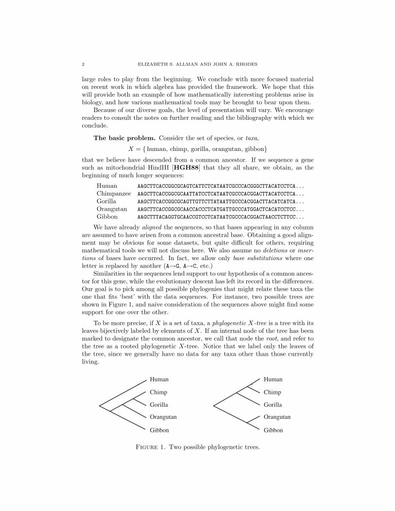
Similarities in the sequences lend support to our hypothesis of a common ances-tor for this gene, while the evolutionary descent has left its record in the differences.Our goal is to pick among all possible phylogenies that might relate these taxa theone that fits ‘best’ with the data sequences. For instance, two possible trees areshown in Figure 1, and naive consideration of the sequences above might find somesupport for one over the other.

To be more precise, if X is a set of taxa, a phylogenetic X-tree is a tree with itsleaves bijectively labeled by elements of X. If an internal node of the tree has beenmarked to designate the common ancestor, we call that node the root, and refer tothe tree as a rooted phylogenetic X-tree. Notice that we label only the leaves ofthe tree, since we generally have no data for any taxa other than those currentlyliving.

Human

Chimp

Gibbon

Gorilla

Orangutan

Human

Chimp

Gibbon

Gorilla

Orangutan

Figure 1. Two possible phylogenetic trees.

PHYLOGENETICS 3

It is common in biology to focus on binary trees (i.e., trivalent, except bivalentat a root) as being of primary interest. Most speciation events are believed to beof the sort where only two species at a time arise from a parent species. Whilemultifurcations in a tree might be used to represent ignorance (so-called soft poly-tomies), such as when several speciation events occurred so closely in time we areunable to resolve their order, they seldom are believed to represent the true history.For the remainder of this chapter, we consider only binary trees.

The large number of possible trees relating n taxa will turn out to be problem-atic for most methods of phylogenetic inference. This is quantified in the followingbasic combinatorial result, easily proved by induction.

Theorem 1.1. If |X| = n, then there are (2n−5)!! = 1 ·3 ·5 · · · (2n−5) distinctunrooted binary phylogenetic X-trees, and (2n− 3)!! distinct rooted ones.

Before determining a tree that best fits the data we must of course specify whatwe mean by ‘best fits.’ There are many approaches to this, and in the next fewsections we highlight those that have played the most important roles.

We should add that information in sequences other than base changes canbe used to infer phylogenies. Genomes occasionally undergo large scale changes,in which genes may be reordered, duplicated, or lost. Because these changes arerarer, they are all useful for inference much further back in evolutionary time thanthe base changes we focus on here.

2. Parsimony

One natural criterion for choosing an optimal tree is to find one that requiresthe fewest base substitutions. The most parsimonious tree (or trees) achieves thisminimum, and at least in circumstances when substitutions are rare is a reasonablecandidate for the best inferred evolutionary history.

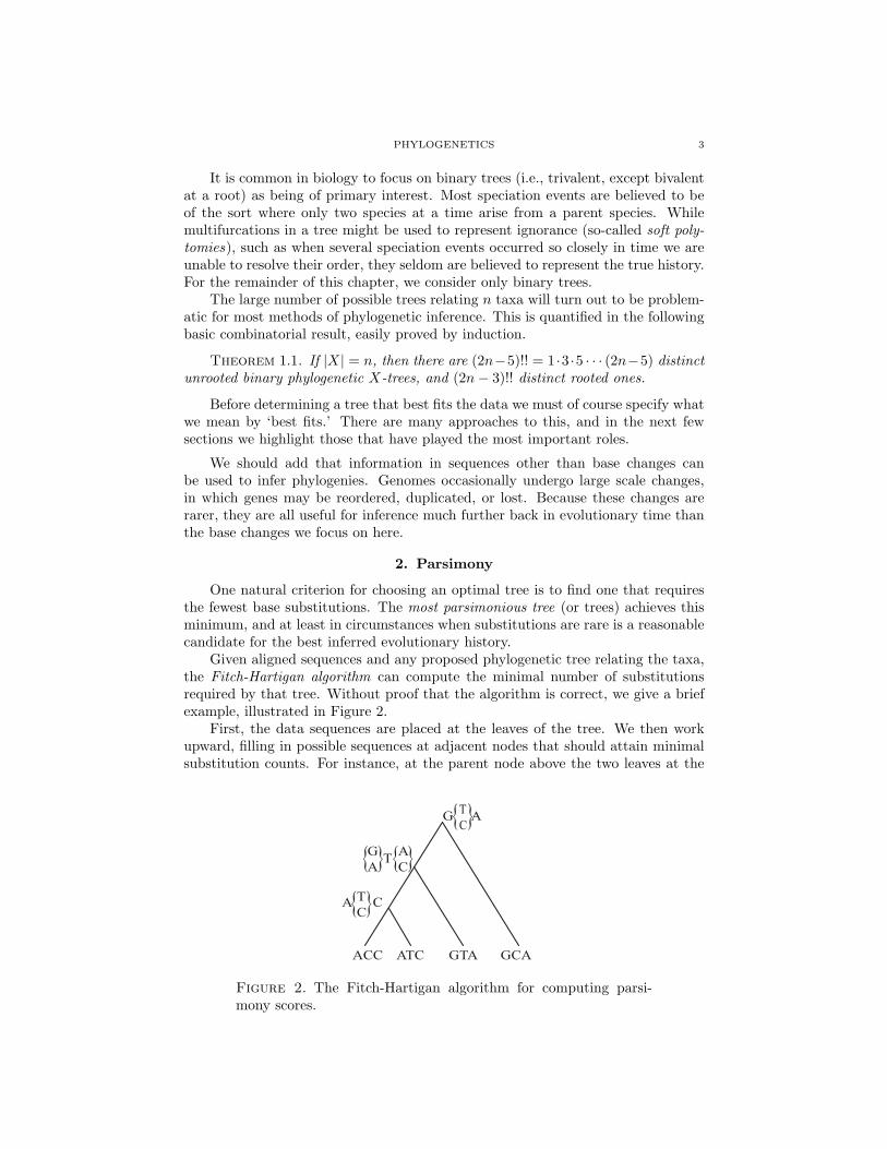
Given aligned sequences and any proposed phylogenetic tree relating the taxa,the Fitch-Hartigan algorithm can compute the minimal number of substitutionsrequired by that tree. Without proof that the algorithm is correct, we give a briefexample, illustrated in Figure 2.

First, the data sequences are placed at the leaves of the tree. We then workupward, filling in possible sequences at adjacent nodes that should attain minimalsubstitution counts. For instance, at the parent node above the two leaves at the

ACC ATC GTA GCA

T

CA C

G

A

A

CT

{ }

G AT

C

{ } { }

{ }

Figure 2. The Fitch-Hartigan algorithm for computing parsi-mony scores.

4 ELIZABETH S. ALLMAN AND JOHN A. RHODES

far left, writing either ATC or ACC would each require only 1 substitution, and we

can do no better. We label this node with A{ TC} C, and count that one mutation

has occurred. Proceeding to its parent, placing a T in the center site requires noadditional substitutions since a T might have occurred in both sequences below it.At the first and third sites, however, substitutions were needed, and all possibilitiesrequiring only 1 substitution per site are listed. So far our substitution count is 3.By filling in sequences at the root, we find we need 1 more substitution, for a totalcount of 4 for this tree. Thus, 4 is the parsimony score of this tree.

The procedure is summarized by: For each node, look at the sequences at itstwo children. At sites where there are no bases in common, write the union of thesets appearing at the children and increase the substitution count by 1. At siteswhere there are bases in common, write the intersection of the sets appearing atthe children and do not change the substitution count.

Two points should be made that may not be clear from this example: 1) theminimal number of substitutions is independent of root location, so parsimonycompares only unrooted trees, and 2) Though it does produce the correct minimalsubstitution count, the algorithm does not reconstruct all ancestral sequences thatachieve the minimal count on the tree. Additional steps are needed to do that, ifdesired.

The Fitch-Hartigan algorithm is fast, in fact O(|X|L), where L is the numberof sites in the sequences. Unfortunately, this is for only one tree, though, andperforming it on all trees is more problematic.

Theorem 2.1 (Foulds and Graham, [FG82]). Determining the most parsimo-nious tree is NP-hard.

Branch and bound approaches to searching tree space are sometimes effective,and many heuristics for good searching have been developed and implemented insoftware. These are believed to perform well in practice, but for a large data set,one never knows for sure that a most parsimonious tree has been found.

A serious problem with parsimony, however, concerns its basic criterion. Sup-pose that along a single edge of a tree a site evolved as A→C→T. The parsimonycriterion would, at best, recognize only one substitution as having occurred. Evenworse, for A→C→A it would count no substitutions. If such hidden mutations orback substitutions occurred, parsimony can be misled.

In fact, using a simple probabilistic model of the substitution process on asmall tree (of the sort to be discussed in Section 4) Felsenstein was able to showthe following.

Theorem 2.2 (Felsenstein, [Fel78]). If multiple mutations can occur at a sitealong any given edge, then there are plausible assumptions under which parsimonywill infer the incorrect tree.

Of course any method of inference may perform poorly when given insufficientdata. Felsenstein’s result concerns the method’s statistical inconsistency : Even asthe amount of data in accord with the model grows without bound, the wrong treeis inferred.

The inconsistency of parsimony is disturbing to the statistically minded. Nonethe-less, parsimony is still in use for inference of trees, though it is not the most popular

PHYLOGENETICS 5

method. As long as hidden mutations are believed to be rare, it may be a reasonableapproach.

3. Distance methods

The next class of methods share with parsimony a combinatorial flavor. Webegin by measuring pairwise dissimilarity between taxa, perhaps by using the Ham-ming distance between their sequences,

d(a, b) =number of sites differing between a and b

total number of sites.

We then seek a metric tree, where each edge has a non-negative length (or weight),so that cumulative lengths along the tree between taxa (values of the tree metric)are close to the dissimilarity values. We view d(a, b) as some sort of measure of howmuch mutation must have occurred along all edges of the tree between a and b.

Note that we do not refer to the dissimilarity d as a distance or metric, sincewe should not expect it to agree with a tree metric exactly. Indeed, since we have afinite amount of data (and assuming we believe some stochastic process lies behindit), it will vary from any idealization due to its finiteness and inadequacies of ourmodel. In addition, the Hamming dissimilarity suffers from the same fundamentalproblem as parsimony — it is insensitive to hidden mutations. After probabilisticmodels are formalized in Section 4, we will be able to address this last point withimproved dissimilarity maps.

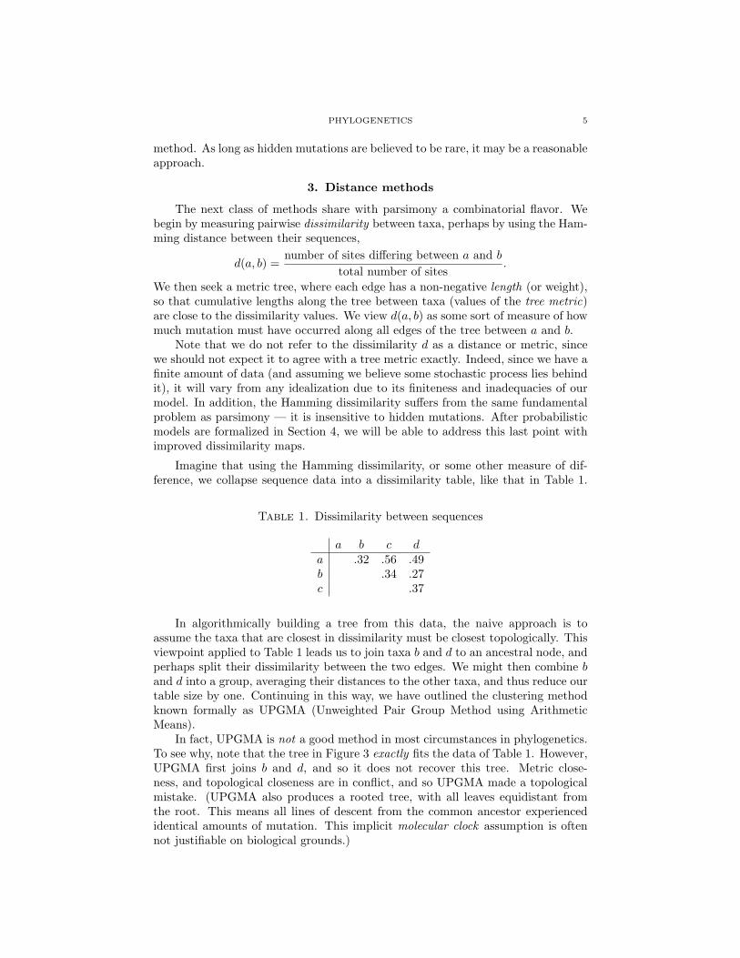
Imagine that using the Hamming dissimilarity, or some other measure of dif-ference, we collapse sequence data into a dissimilarity table, like that in Table 1.

Table 1. Dissimilarity between sequences

a b c da .32 .56 .49b .34 .27c .37

In algorithmically building a tree from this data, the naive approach is toassume the taxa that are closest in dissimilarity must be closest topologically. Thisviewpoint applied to Table 1 leads us to join taxa b and d to an ancestral node, andperhaps split their dissimilarity between the two edges. We might then combine band d into a group, averaging their distances to the other taxa, and thus reduce ourtable size by one. Continuing in this way, we have outlined the clustering methodknown formally as UPGMA (Unweighted Pair Group Method using ArithmeticMeans).

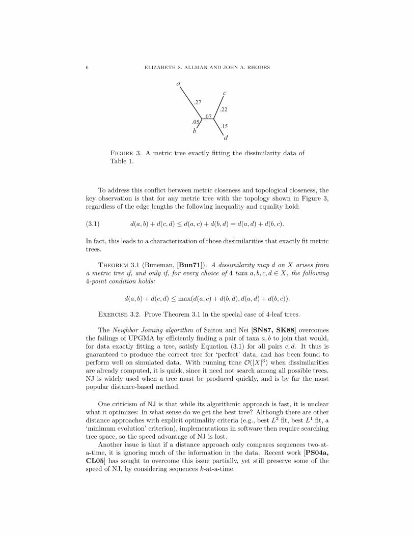
In fact, UPGMA is not a good method in most circumstances in phylogenetics.To see why, note that the tree in Figure 3 exactly fits the data of Table 1. However,UPGMA first joins b and d, and so it does not recover this tree. Metric close-ness, and topological closeness are in conflict, and so UPGMA made a topologicalmistake. (UPGMA also produces a rooted tree, with all leaves equidistant fromthe root. This means all lines of descent from the common ancestor experiencedidentical amounts of mutation. This implicit molecular clock assumption is oftennot justifiable on biological grounds.)

6 ELIZABETH S. ALLMAN AND JOHN A. RHODES

a

b

c

d

.27

.07

.22

.05.15

Figure 3. A metric tree exactly fitting the dissimilarity data ofTable 1.

To address this conflict between metric closeness and topological closeness, thekey observation is that for any metric tree with the topology shown in Figure 3,regardless of the edge lengths the following inequality and equality hold:

(3.1) d(a, b) + d(c, d) ≤ d(a, c) + d(b, d) = d(a, d) + d(b, c).

In fact, this leads to a characterization of those dissimilarities that exactly fit metrictrees.

Theorem 3.1 (Buneman, [Bun71]). A dissimilarity map d on X arises froma metric tree if, and only if, for every choice of 4 taxa a, b, c, d ∈ X, the following4-point condition holds:

d(a, b) + d(c, d) ≤ max(d(a, c) + d(b, d), d(a, d) + d(b, c)).

Exercise 3.2. Prove Theorem 3.1 in the special case of 4-leaf trees.

The Neighbor Joining algorithm of Saitou and Nei [SN87, SK88] overcomesthe failings of UPGMA by efficiently finding a pair of taxa a, b to join that would,for data exactly fitting a tree, satisfy Equation (3.1) for all pairs c, d. It thus isguaranteed to produce the correct tree for ‘perfect’ data, and has been found toperform well on simulated data. With running time O(|X|3) when dissimilaritiesare already computed, it is quick, since it need not search among all possible trees.NJ is widely used when a tree must be produced quickly, and is by far the mostpopular distance-based method.

One criticism of NJ is that while its algorithmic approach is fast, it is unclearwhat it optimizes: In what sense do we get the best tree? Although there are otherdistance approaches with explicit optimality criteria (e.g., best L2 fit, best L1 fit, a‘minimum evolution’ criterion), implementations in software then require searchingtree space, so the speed advantage of NJ is lost.

Another issue is that if a distance approach only compares sequences two-at-a-time, it is ignoring much of the information in the data. Recent work [PS04a,CL05] has sought to overcome this issue partially, yet still preserve some of thespeed of NJ, by considering sequences k-at-a-time.

PHYLOGENETICS 7

a1

a2

an

a3a4

r

Figure 4. An n-taxon tree.

4. Base Substitution Models

Before going further with our survey of common phylogenetic methods, wemust introduce some of the probabilistic models of molecular evolution which othermethods use. Explicit models allow a firmer grounding in statistical theory.

Most probabilistic models of the mutation process focus on a single site in asequence, and only on base substitutions occurring at that site as evolution proceedsdown a tree. Other types of sequence changes — insertions, deletions, inversions— require more complicated models than will be discussed here.

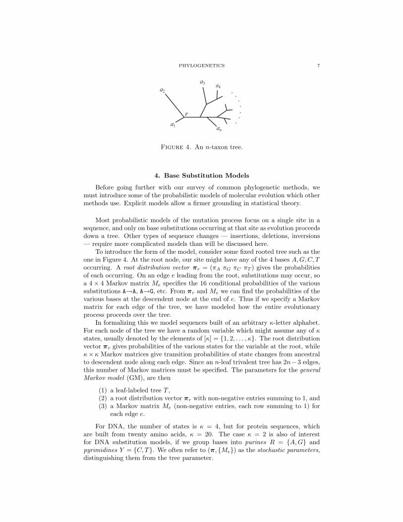
To introduce the form of the model, consider some fixed rooted tree such as theone in Figure 4. At the root node, our site might have any of the 4 bases A,G, C, Toccurring. A root distribution vector πr = (πA πG πC πT ) gives the probabilitiesof each occurring. On an edge e leading from the root, substitutions may occur, soa 4× 4 Markov matrix Me specifies the 16 conditional probabilities of the varioussubstitutions A→A, A→G, etc. From πr and Me we can find the probabilities of thevarious bases at the descendent node at the end of e. Thus if we specify a Markovmatrix for each edge of the tree, we have modeled how the entire evolutionaryprocess proceeds over the tree.

In formalizing this we model sequences built of an arbitrary κ-letter alphabet.For each node of the tree we have a random variable which might assume any of κstates, usually denoted by the elements of [κ] = {1, 2, . . . , κ}. The root distributionvector πr gives probabilities of the various states for the variable at the root, whileκ× κ Markov matrices give transition probabilities of state changes from ancestralto descendent node along each edge. Since an n-leaf trivalent tree has 2n−3 edges,this number of Markov matrices must be specified. The parameters for the generalMarkov model (GM), are then

(1) a leaf-labeled tree T ,(2) a root distribution vector πr with non-negative entries summing to 1, and(3) a Markov matrix Me (non-negative entries, each row summing to 1) for

each edge e.

For DNA, the number of states is κ = 4, but for protein sequences, whichare built from twenty amino acids, κ = 20. The case κ = 2 is also of interestfor DNA substitution models, if we group bases into purines R = {A,G} andpyrimidines Y = {C, T}. We often refer to (π, {Me}) as the stochastic parameters,distinguishing them from the tree parameter.

8 ELIZABETH S. ALLMAN AND JOHN A. RHODES

a1

a2

a3

a4

v w

M1

M2

M3M4

M5

Figure 5. Computing the expected pattern frequencies on T .

A key point in the use of a model such as this is that while it describes statesat all nodes of the tree, in fact only those at the leaves are observable, since theleaves represent the extant taxa from which we may obtain data.

With the parameters of the model thus specified, we are interested in the jointdistribution P of states at the leaves a1, a2, . . . , an. The joint distribution P is ann-dimensional κ× · · · × κ tensor (or table or array) with entries

P (i1, · · · , in) = Prob(a1 = ii, · · · , an = in).

The entries of P then are the expected frequencies of observing a pattern of statessuch as (i1, · · · , in) at the leaves of the tree. These expected pattern frequenciescan be explicitly expressed in terms of the parameters of the model, as we explainthrough an example.

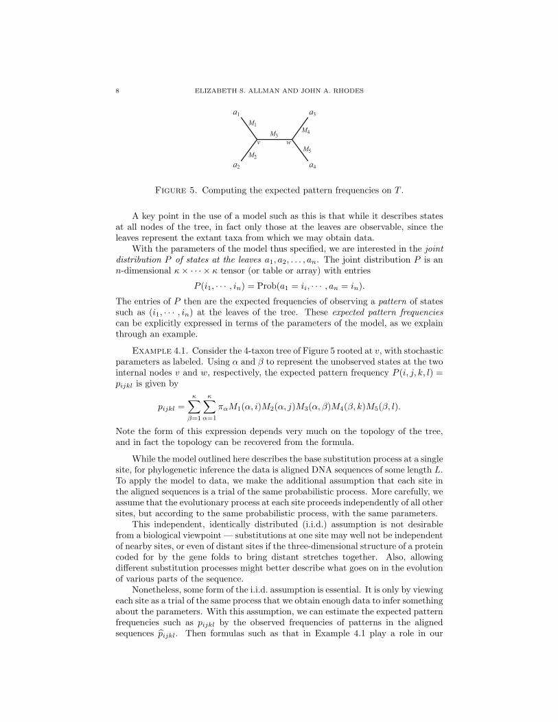
Example 4.1. Consider the 4-taxon tree of Figure 5 rooted at v, with stochasticparameters as labeled. Using α and β to represent the unobserved states at the twointernal nodes v and w, respectively, the expected pattern frequency P (i, j, k, l) =pijkl is given by

pijkl =κ∑

β=1

κ∑α=1

παM1(α, i)M2(α, j)M3(α, β)M4(β, k)M5(β, l).

Note the form of this expression depends very much on the topology of the tree,and in fact the topology can be recovered from the formula.

While the model outlined here describes the base substitution process at a singlesite, for phylogenetic inference the data is aligned DNA sequences of some length L.To apply the model to data, we make the additional assumption that each site inthe aligned sequences is a trial of the same probabilistic process. More carefully, weassume that the evolutionary process at each site proceeds independently of all othersites, but according to the same probabilistic process, with the same parameters.

This independent, identically distributed (i.i.d.) assumption is not desirablefrom a biological viewpoint — substitutions at one site may well not be independentof nearby sites, or even of distant sites if the three-dimensional structure of a proteincoded for by the gene folds to bring distant stretches together. Also, allowingdifferent substitution processes might better describe what goes on in the evolutionof various parts of the sequence.

Nonetheless, some form of the i.i.d. assumption is essential. It is only by viewingeach site as a trial of the same process that we obtain enough data to infer somethingabout the parameters. With this assumption, we can estimate the expected patternfrequencies such as pijkl by the observed frequencies of patterns in the alignedsequences pijkl. Then formulas such as that in Example 4.1 play a role in our

PHYLOGENETICS 9

a1 a2

Figure 6. A 2-taxon tree.

inference of the root distribution, Markov matrices, and most importantly, thetree.

We now wish to show that for most parameter choices we can produce the samejoint distribution at the leaves of a tree as we could with a different root locationand a related choice of parameters.

To develop this idea, first consider the 2-taxon tree of Figure 6, with a1 desig-nated as the root. Let πa1 = (π1 π2 π3 π4) be the root distribution vector, and, fore = (a1 → a2), let

Me = (mij) , mij = Prob(a2 = j | a1 = i),

be the matrix of conditional probabilities of base substitutions along the edge.To compute the joint distribution P = Pa1a2 , a 4×4 matrix of expected pattern

frequencies, notice that the (i, j)-entry pij is πimij , or in matrix form,

(4.1) Pa1a2 = diag(πa1)Me =

π1m11 π1m12 π1m13 π1m14

π2m21 π2m22 π2m23 π2m24

π3m31 π3m32 π3m33 π3m34

π4m41 π4m42 π4m43 π4m44

,

where diag(πa1) denotes the diagonal matrix with entries from πa1 .Now consider the same 2-taxon tree T in Figure 6, but with the root taken at

a2 instead. Then in terms of the stochastic parameters on T rooted at a1, define theroot distribution vector to be πa2 = πa1Me, the probabilities that leaf a2 is in eachof the four states. Let Me′ denote a Markov transition matrix for e′ = (a2 → a1)that will be determined shortly.

Notice that viewing a2 as the root, the joint distribution is expressed as Pa2a1 =(Pa1a2)

T . Thus we would like to find Me′ so that,

diag(πa2)Me′ = Pa2a1 = (Pa1a2)T = (diag(πa1)Me)

T = MTe diag(πa1).

If the entries of πa2 are all positive, then we may take

Me′ = diag(πa2)−1

MTe diag(πa1).

This establishes that, under mild conditions, there is a choice of parameters for Trooted at a2 that give rise to the same joint distribution P as the parameters πa1

and Me for T rooted at a1. Hence, for the general Markov model, we can ‘move theroot’ without affecting the entries of the joint distribution array P . We formalizethese observations and extend the setting to n-taxon trees in Proposition 4.2.

Proposition 4.2. Fix an n-taxon tree T . Let r be some choice of root for T(which may be a leaf, an internal node of valance 3, or along some edge). Then,for generic choices of stochastic parameters Sr for the general Markov model rootedat r, and for any other choice of a root s for T at either a leaf or an internalnode of valance 3, there is a uniquely determined choice of general Markov model

10 ELIZABETH S. ALLMAN AND JOHN A. RHODES

parameters Ss for the model rooted at s producing the same joint distribution at theleaves as Sr.

A consequence of Proposition 4.2 is that the location of the root in a tree Tis a biological problem, not a mathematical one. Under this model (and manyothers as well), there is no way to mathematically identify a node in T as a mostrecent common ancestor of the taxa in hand. (However by including an outgroup,a taxon known to be distantly related to those under study, one can use biologicalknowledge to locate a root.)

For this reason, we usually consider the inference of an unrooted tree as ourgoal. In addition, for computations with a model, and in arguments, we are nowfree to place roots wherever we find most convenient.

While the general Markov model is simple to explain, it has more parametersthan models typically used in practice. Once the tree parameter has been chosenas a particular n-taxon tree, there are κ− 1 free choices to be made for πr, and foreach of the 2n − 3 edges, κ(κ − 1) free choices for entries in Me, giving a total ofκ− 1 + (2n− 3)κ(κ− 1) numerical parameters. Though this grows only linearly inthe number of taxa, the coefficient is rather large. For κ = 4, the total number ofparameters is already roughly 24n.

This large number of parameters has two effects. First, it slows down compu-tations, which for a large number of sequences can be problematic. Second, usinga parameter-rich model allows us to better fit data, but may also allow overfitting.If the data can be described by a model with fewer parameters, that model mayprovide a better basis for inference.

Restrictions on the particular form of the stochastic parameters, some arisingfrom biological considerations and some for mathematical convenience, give rise tosubmodels of the GM model. We discuss these, as well as some extensions to moreelaborate models next.

Group-based models. The Jukes-Cantor model for DNA is the biologically-plausible model with the fewest parameters. It assumes a uniform root distributionvector of π = (.25 .25 .25 .25) and edge transition matrices of the form

MJC =

1− a a3

a3

a3

a3 1− a a

3a3

a3

a3 1− a a

3a3

a3

a3 1− a

,

where a different value of a may be used for each edge. On each edge, all non-identical base substitutions are equally likely, and the probability that some changeoccurs at a site between the endpoints of the edge is given by the parameter a.Note that the root distribution is an eigenvector of MJC , so a uniform distributionof states will occur at each node in the tree.

Though this model is attractive for its simplicity, further realism can be in-troduced by having two probabilities of changes, as we now describe. Because ofchemical similarities, the bases are classified as purines {A,G} and pyrimidines{C, T}. Assigning probability a to in-class changes (transitions), and b to out-of-class changes (transversions), we arrive at the Kimura 2-parameter model, with

PHYLOGENETICS 11

matrices

MK2P =

1− (a + 2b) a b ba 1− (a + 2b) b bb b 1− (a + 2b) ab b a 1− (a + 2b)

,

where the rows and columns are ordered by the states A, G, C, T , (purines, fol-lowed by pyrimidines). Typically a > b, since transitions are often observed morefrequently than transversions.

A slight generalization, introduced more for its mathematical structure thanfor biological reasons, is the Kimura 3-parameter model with transition matrices ofthe form

MK3P =

1− (a + b + c) a b ca 1− (a + b + c) c bb c 1− (a + b + c) ac b a 1− (a + b + c)

.

Notice the pattern to the entries is that of an addition table for the groupZ2 × Z2. In fact, if we identify the four bases with group elements by

A = (0, 0), G = (1, 0), C = (0, 1), T = (1, 1),

then a substitution X → Y is naturally encoded by the group element Y − Xsince X + (Y −X) = Y . If a random choice of a group element determines whatsubstitution occurs, then the numbers 1 − (a + b + c), a, b, and c represent theprobabilities of each choice, explaining the form of MK3P .

This special structure has produced some quite interesting results for the K3Pmodel, and its specializations, the K2P and JC models. Although we will notexplain it here, the Hadamard conjugation of [Hen89, HP89] is a fundamentalresult that introduced Fourier analysis as a tool for studying such models. Thiswas further developed in [SSE93].

General Time Reversible models. So far we’ve essentially taken a discretetime approach to modeling substitutions, by specifying transition probabilities re-lating states at the two ends of an edge. Substitutions may also be modeled asa continuous time process. In fact, if we are interested in inferring elapsed timebetween speciation events, we must take this approach so that those times becomeparameters.

To formulate a continuous time model, we let Q denote a κ× κ instantaneousrate matrix. The off-diagonal entries of Q represent rates at which the 12 non-identical substitutions occur, and are thus non-negative numbers. The diagonalentries are chosen so that the rows sum to zero. Associated to each edge e of Tis a parameter te, an edge length. If e = (v → w), then te represents the amountof time elapsed during evolution of the sequence at v into the sequence at w. TheMarkov transition matrix for e is then the matrix exponential, Me = exp(Qte).

When using continuous time models, we generally choose one rate matrix Qfor all edges of the tree. This imposes some commonality to the evolutionaryprocess on all edges of the tree that is biologically reasonable in some (but notall) circumstances. It also dramatically reduces the dependency of the number ofparameters of the model on the number n of taxa to roughly 2n, since that is the

12 ELIZABETH S. ALLMAN AND JOHN A. RHODES

growth rate of the number of edges, and we add only one new parameter, te, foreach edge.

It’s usually most convenient to require that the root distribution vector π = πr

be an eigenvector of Q with eigenvalue 0. This ensures that π is an eigenvector ofMe = exp(Qte) with eigenvalue 1, for all values of te. As a result, the model is astationary one, with state distribution the same at all nodes of the tree.

Along with this we often assume time-reversibility :

diag(π)Q = QT diag(π).

Imposing this condition, that diag(π)Q is symmetric, implies that diag (π) exp(Qte)is symmetric for all te. But we saw in Equation (4.1) that diag (π) exp (Qte) rep-resents the joint distribution of states at the two ends of e. Therefore, stationaritywith time-reversibility means that we can use the same parameters π, Q, te to modelevolution on an edge regardless of the orientation of the edge.

The general time-reversible (GTR) model is a rate-matrix model making boththe stationarity and time-reversible assumptions. These assumptions imply we can‘move the root’ in a tree under the GTR model without affecting the entries of thejoint distribution P . As with the GM model, we will not be able to mathematicallydetermine a root location when we use the GTR model for inference. This isconvenient, since it means for inference we will not have to search over all rootedtrees, but rather over unrooted ones. In fact, the reason the GTR model is used isprecisely that it is the most general rate-matrix model with this property.

Exercise 4.3. Show that all pairs π, Q for the κ-state GTR model can bespecified by formulas involving (κ − 1) + κ(κ − 1)/2 scalar parameters, and thus,after normalizing so that one edge has length 1, the GTR model on an n-taxon treehas (κ− 1) + κ(κ− 1)/2 + (2n− 4) parameters.

Exercise 4.4. Show that the JC model is a special case of GTR, by findingπ, QJC explicitly.

Exercise 4.5. Show that the K2P model may be a special case of GTR, butthat there are choices of K2P parameters that are not instances of a GTR model.More specifically, find π and all possible Q so that Me = exp(Qte) are K2P edgetransition matrices. Then find a relationship between the sets of eigenvalues of Me,for each of the 2n− 3 edges e, that must hold if an arbitrary K2P model is a GTRmodel.

Exercise 4.6. Consider the 2-taxon tree of Figure 6 rooted at a1. If πa1 =

(.23 .26 .24 .27) and Ma1a2 =

.96 .02 .01 .01

.06 .88 .02 .04

.01 .04 .93 .02

.05 .05 .04 .86

, compute the joint distribu-

tion of bases at the leaves P = Pa1a2 . Could this come from the GTR model?

Mixture models. It is unrealistic biologically to assume that all sites mutateaccording to the same process. Certainly it is plausible that non-coding regionsof the genome might undergo substitutions at a faster rate than coding ones. Buteven within genes, there may be variability.

PHYLOGENETICS 13

Triplets of bases form codons that specify an amino acid to appear in theprotein molecule for which the gene encodes, but the genetic code which relatescodons to amino acids has redundancy. There are 43 possible codons, but only 20amino acids. Much of the redundancy of the code is such that different bases inthe third codon position may not affect the gene product. Thus the third positionmay be more likely to experience a higher mutation rate.

Moreover, since some parts of the protein structures might be essential to theviability of an organism, those sites coding for such parts may never be observedto undergo any substitutions at all. Typically, then, we expect variability in themutation process among sites, but do not know how to partition the sites intovarious classes according to their behavior.

A step toward improving our description of molecular evolution then is tointroduce a mixture model. In this formulation, each site in aligned sequences fallsinto one of k classes and each of the k classes carries its own stochastic parameters.Of course all sites share the same tree parameter. An additional k − 1 parametersδi are needed to indicate the proportion of the sites that lie in the ith class, i =1, · · · , k − 1, with δk = 1−∑k−1

i=1 δi giving the proportion in the last class.

For example, consider a situation in which some sites in our sequences arebelieved to be unable to undergo substitutions, perhaps because of functional con-straints on a protein product. We call these invariable sites. Notice that in aligningsequences we usually have many sites that are in complete agreement, but we donot necessarily believe they were invariable — they may have been able to undergosubstitutions, but simply did not. If we believe invariable sites exist, then we can-not directly distinguish between the constant sites which are invariable and thosewhich were free to vary but did not.

To model this, we introduce the GM+I model. For a fixed rooted tree, theparameters are 1) For the sites that can vary, a root distribution vector πGM

and Markov matrices {Me} for each edge of the tree, 2) For those sites that areinvariable, a root distribution vector πI , and 3) a mixing parameter δ indicatingthe proportion of sites that mutate according to a GM process. The resulting jointdistribution P is a weighted sum

PGM+I = δPGM + (1− δ)PI ,

where PGM is the joint distribution for the varying sites, and PI the joint dis-tribution for the invariable sites, an n-dimensional diagonal tensor formed fromπI .

GM+I is just one of many mixture models that can incorporate more biolog-ical realism in modeling the base substitution process, and this example shouldmake clear what we mean by mixture models such as GM+GM+GM, GM+GM+I,GTR+I, or JC+I.

The use of mixture models can greatly increase the number of stochastic pa-rameters. For a k-class general Markov mixture model, for instance, the number ofstochastic parameters increases by more than a factor of k. While mixture modelsare appealing since they conform better with our intuitive notion of how to modelbase substitutions, the large number of parameters increases the risk of overfittingdata. At the extreme, one might imagine a mixture model with so many classesthat, for appropriate parameter choices, it might be capable of producing any jointdistribution at all. If such a model describes data, then we have no hope of inferring

14 ELIZABETH S. ALLMAN AND JOHN A. RHODES

a tree, since no signal indicating the correct tree can be found in the observed jointdistribution.

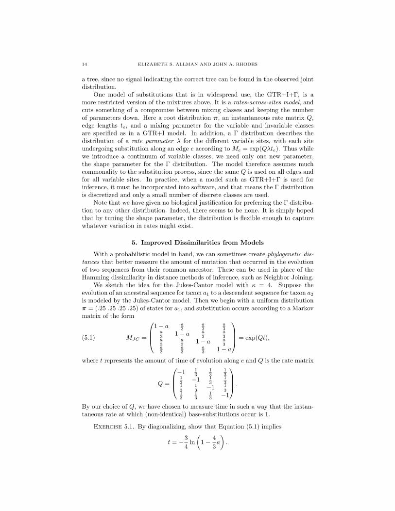
One model of substitutions that is in widespread use, the GTR+I+Γ, is amore restricted version of the mixtures above. It is a rates-across-sites model, andcuts something of a compromise between mixing classes and keeping the numberof parameters down. Here a root distribution π, an instantaneous rate matrix Q,edge lengths te, and a mixing parameter for the variable and invariable classesare specified as in a GTR+I model. In addition, a Γ distribution describes thedistribution of a rate parameter λ for the different variable sites, with each siteundergoing substitution along an edge e according to Me = exp(Qλte). Thus whilewe introduce a continuum of variable classes, we need only one new parameter,the shape parameter for the Γ distribution. The model therefore assumes muchcommonality to the substitution process, since the same Q is used on all edges andfor all variable sites. In practice, when a model such as GTR+I+Γ is used forinference, it must be incorporated into software, and that means the Γ distributionis discretized and only a small number of discrete classes are used.

Note that we have given no biological justification for preferring the Γ distribu-tion to any other distribution. Indeed, there seems to be none. It is simply hopedthat by tuning the shape parameter, the distribution is flexible enough to capturewhatever variation in rates might exist.

5. Improved Dissimilarities from Models

With a probabilistic model in hand, we can sometimes create phylogenetic dis-tances that better measure the amount of mutation that occurred in the evolutionof two sequences from their common ancestor. These can be used in place of theHamming dissimilarity in distance methods of inference, such as Neighbor Joining.

We sketch the idea for the Jukes-Cantor model with κ = 4. Suppose theevolution of an ancestral sequence for taxon a1 to a descendent sequence for taxon a2

is modeled by the Jukes-Cantor model. Then we begin with a uniform distributionπ = (.25 .25 .25 .25) of states for a1, and substitution occurs according to a Markovmatrix of the form

(5.1) MJC =

1− a a3

a3

a3

a3 1− a a

3a3

a3

a3 1− a a

3a3

a3

a3 1− a

= exp(Qt),

where t represents the amount of time of evolution along e and Q is the rate matrix

Q =

−1 13

13

13

13 −1 1

313

13

13 −1 1

313

13

13 −1

.

By our choice of Q, we have chosen to measure time in such a way that the instan-taneous rate at which (non-identical) base-substitutions occur is 1.

Exercise 5.1. By diagonalizing, show that Equation (5.1) implies

t = −34

ln(

1− 43a

).

PHYLOGENETICS 15

Since a represents the probability of a (non-identical) substitution being ob-served when we compare a site in the sequences for a1 and a2, we can estimate a bythe Hamming distance between the sequences, a. We thus define the Jukes-Cantordistance between the sequences as

dJC(a1, a2) = −34

ln(

1− 43a

).

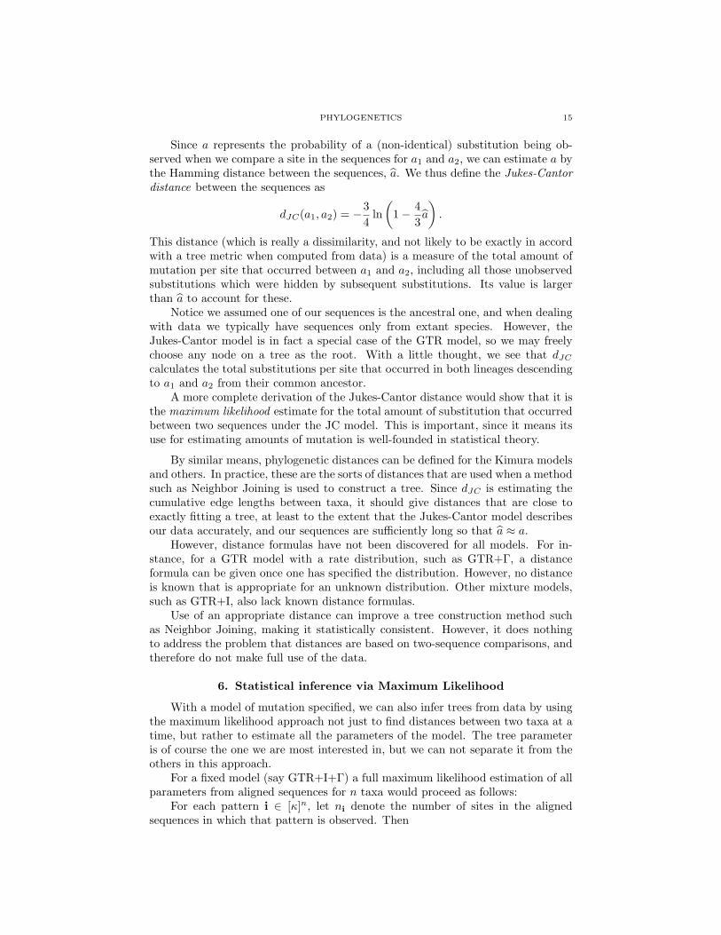
This distance (which is really a dissimilarity, and not likely to be exactly in accordwith a tree metric when computed from data) is a measure of the total amount ofmutation per site that occurred between a1 and a2, including all those unobservedsubstitutions which were hidden by subsequent substitutions. Its value is largerthan a to account for these.

Notice we assumed one of our sequences is the ancestral one, and when dealingwith data we typically have sequences only from extant species. However, theJukes-Cantor model is in fact a special case of the GTR model, so we may freelychoose any node on a tree as the root. With a little thought, we see that dJC

calculates the total substitutions per site that occurred in both lineages descendingto a1 and a2 from their common ancestor.

A more complete derivation of the Jukes-Cantor distance would show that it isthe maximum likelihood estimate for the total amount of substitution that occurredbetween two sequences under the JC model. This is important, since it means itsuse for estimating amounts of mutation is well-founded in statistical theory.

By similar means, phylogenetic distances can be defined for the Kimura modelsand others. In practice, these are the sorts of distances that are used when a methodsuch as Neighbor Joining is used to construct a tree. Since dJC is estimating thecumulative edge lengths between taxa, it should give distances that are close toexactly fitting a tree, at least to the extent that the Jukes-Cantor model describesour data accurately, and our sequences are sufficiently long so that a ≈ a.

However, distance formulas have not been discovered for all models. For in-stance, for a GTR model with a rate distribution, such as GTR+Γ, a distanceformula can be given once one has specified the distribution. However, no distanceis known that is appropriate for an unknown distribution. Other mixture models,such as GTR+I, also lack known distance formulas.

Use of an appropriate distance can improve a tree construction method suchas Neighbor Joining, making it statistically consistent. However, it does nothingto address the problem that distances are based on two-sequence comparisons, andtherefore do not make full use of the data.

6. Statistical inference via Maximum Likelihood

With a model of mutation specified, we can also infer trees from data by usingthe maximum likelihood approach not just to find distances between two taxa at atime, but rather to estimate all the parameters of the model. The tree parameteris of course the one we are most interested in, but we can not separate it from theothers in this approach.

For a fixed model (say GTR+I+Γ) a full maximum likelihood estimation of allparameters from aligned sequences for n taxa would proceed as follows:

For each pattern i ∈ [κ]n, let ni denote the number of sites in the alignedsequences in which that pattern is observed. Then

16 ELIZABETH S. ALLMAN AND JOHN A. RHODES

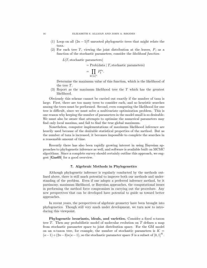
(1) Loop on all (2n − 5)!! unrooted phylogenetic trees that might relate thetaxa.

(2) For each tree T , viewing the joint distribution at the leaves, P , as afunction of the stochastic parameters, consider the likelihood function

L(T, stochastic parameters)

= Prob(data | T, stochastic parameters)

=∏

i∈[κ]n

Pni

i .

Determine the maximum value of this function, which is the likelihood ofthe tree T .

(3) Report as the maximum likelihood tree the T which has the greatestlikelihood.

Obviously this scheme cannot be carried out exactly if the number of taxa islarge. First, there are too many trees to consider each, and so heuristic searchesamong the trees must be performed. Second, even computing the likelihood for onetree is difficult, since we must solve a multivariate optimization problem. This isone reason why keeping the number of parameters in the model small is so desirable.We must also be aware that attempts to optimize the numerical parameters mayfind only local maxima, and fail to find the true global maximum.

Nonetheless, computer implementations of maximum likelihood inference areheavily used because of the desirable statistical properties of the method. But asthe number of taxa is increased, it becomes impossible to complete the searches ina reasonable amount of time.

Recently there has also been rapidly growing interest in using Bayesian ap-proaches to phylogenetic inference as well, and software is available built on MCMCalgorithms. Since a complete survey should certainly outline this approach, we sug-gest [Gas05] for a good overview.

7. Algebraic Methods in Phylogenetics

Although phylogenetic inference is regularly conducted by the methods out-lined above, there is still much potential to improve both our methods and under-standing of the problem. Even if one adopts a preferred inference method, be itparsimony, maximum likelihood, or Bayesian approaches, the computational issuesin performing the method force compromises in carrying out the procedure. Anynew perspectives that can be developed have potential to guide us toward betterapproaches.

In recent years, the perspectives of algebraic geometry have been brought intophylogenetics. Though still very much under development, we turn now to intro-ducing this viewpoint.

Phylogenetic invariants, ideals, and varieties. Consider a fixed n-taxontree T . Then any probabilistic model of molecular evolution on T defines a mapfrom stochastic parameter space to joint distribution space. For the GM modelon an n-taxon tree, for example, the number of stochastic parameters is K =(κ−1)+(2n−3)κ(κ−1), so the stochastic parameter space S is a subset of [0, 1]K .

PHYLOGENETICS 17

Since the joint distribution P is an n-dimensional array, the GM model on T definesa map φT :

φT : S −→ [0, 1]κn

(π, {Me}) 7−→ P.

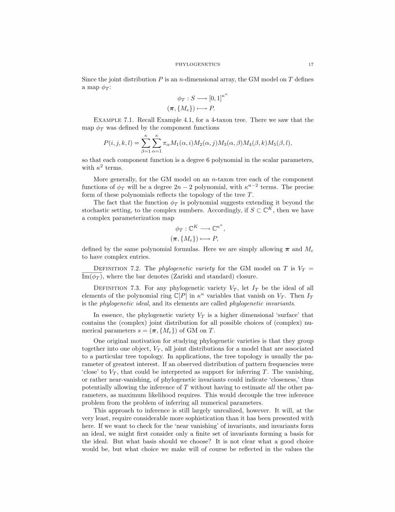
Example 7.1. Recall Example 4.1, for a 4-taxon tree. There we saw that themap φT was defined by the component functions

P (i, j, k, l) =κ∑

β=1

κ∑α=1

παM1(α, i)M2(α, j)M3(α, β)M4(β, k)M5(β, l),

so that each component function is a degree 6 polynomial in the scalar parameters,with κ2 terms.

More generally, for the GM model on an n-taxon tree each of the componentfunctions of φT will be a degree 2n− 2 polynomial, with κn−2 terms. The preciseform of these polynomials reflects the topology of the tree T .

The fact that the function φT is polynomial suggests extending it beyond thestochastic setting, to the complex numbers. Accordingly, if S ⊂ CK , then we havea complex parameterization map

φT : CK −→ Cκn

,

(π, {Me}) 7−→ P,

defined by the same polynomial formulas. Here we are simply allowing π and Me

to have complex entries.

Definition 7.2. The phylogenetic variety for the GM model on T is VT =Im(φT ), where the bar denotes (Zariski and standard) closure.

Definition 7.3. For any phylogenetic variety VT , let IT be the ideal of allelements of the polynomial ring C[P ] in κn variables that vanish on VT . Then IT

is the phylogenetic ideal, and its elements are called phylogenetic invariants.

In essence, the phylogenetic variety VT is a higher dimensional ‘surface’ thatcontains the (complex) joint distribution for all possible choices of (complex) nu-merical parameters s = (π, {Me}) of GM on T .

One original motivation for studying phylogenetic varieties is that they grouptogether into one object, VT , all joint distributions for a model that are associatedto a particular tree topology. In applications, the tree topology is usually the pa-rameter of greatest interest. If an observed distribution of pattern frequencies were‘close’ to VT , that could be interpreted as support for inferring T . The vanishing,or rather near-vanishing, of phylogenetic invariants could indicate ‘closeness,’ thuspotentially allowing the inference of T without having to estimate all the other pa-rameters, as maximum likelihood requires. This would decouple the tree inferenceproblem from the problem of inferring all numerical parameters.

This approach to inference is still largely unrealized, however. It will, at thevery least, require considerable more sophistication than it has been presented withhere. If we want to check for the ‘near vanishing’ of invariants, and invariants forman ideal, we might first consider only a finite set of invariants forming a basis forthe ideal. But what basis should we choose? It is not clear what a good choicewould be, but what choice we make will of course be reflected in the values the

18 ELIZABETH S. ALLMAN AND JOHN A. RHODES

polynomials take on on data. Naive approaches to judging ‘near vanishing’ for onebasis may not correspond to ‘near vanishing’ for another. And regardless, all ofthis should be grounded in some sort of statistical reasoning so we can understandbetter how it should perform with data.

Remark 7.4. Extending the parameterization φT to the complex numbersfrom the stochastic setting is done because an algebraically closed field providesthe easiest and most natural setting for understanding polynomial maps. Of coursecomplex parameters and complex joint distributions P are not so natural from abiological or statistical viewpoint. As the goal ultimately is to understand the GMmodel in a stochastic setting, a more appropriate setting might be real algebraicgeometry. That study, however, remains for the future.

Also, by taking the closure, some points in VT have been introduced that arenot in the image of the parameterization φT . While this is natural to an algebraicgeometer, we can also justify it in another way. If a point is in this closure, thenthere are points on the parameterized portion of VT that are arbitrarily close to it.If we have an observed joint distribution from data sequences, and we are tryingto determine if it is ‘close’ to the variety, then it makes no difference whether wesee if it is ‘close’ to the parameterized portion of the variety, or to any point on thevariety.

One can of course define phylogenetic varieties and invariants for other models,such as JC or K3P, which have polynomial parameterization maps as well. Formost models, these varieties are irreducible (equivalently, the phylogenetic ideal isprime), but see [AR06] for an exception. We continue to focus on the GM modelfor most of our exposition.

Phylogenetic invariants were introduced independently in two papers, by Caven-der and Felsenstein [CF87], and by Lake [Lak87], both for simpler models thanGM. Lake dealt only with linear invariants, while Cavender and Felsenstein consid-ered higher degree ones as well, and even dealt with some issues of real vs. complexgeometry. Though using no language of algebraic geometry, [CF87] is still anexcellent introduction to the viewpoint.

Finding invariants. The dimension of stochastic parameter space, K, is muchsmaller than the dimension of joint distribution space κn, and as a result thereshould be many polynomials vanishing on VT . How to find them explicitly, though,is not obvious.

But finding phylogenetic invariants is simply an instance of an implicitizationproblem in algebraic geometry: Given a parameterized variety such as VT , with apolynomial parameterization map φT , find an implicit description of it as the zeroset of polynomials. Once we have fixed a choice of model and T , we can writedown explicit formulas for the map φT . Then implicitization can be attemptedcomputationally, as a variable elimination problem using Grobner bases (see, forinstance, [CLO97]).

As long as the model is simple (a small number κ of states and a small numberof parameters), and the tree is small (so the dimension κn of the space in whichVT lies is not too large), this can be done by software such as Maple, Macaulay2[GS02], Singular [GPS01], or other computational algebra packages. However,one quickly reaches the limits of current software as the number of states, the

PHYLOGENETICS 19

number of taxa, or the number of parameters in the model grows. Nonetheless,such calculations are instructive to perform, whether to get a feel for the problem,or for developing conjectures.

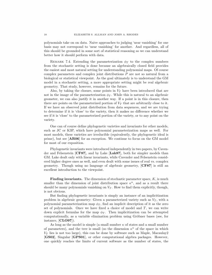
Exercise 7.5. Consider a 2-state model of Jukes-Cantor form, with uniformroot distribution and Markov matrices of the form

Me =(

1− ae ae

ae 1− ae

)

on a 4-leaf tree. Using a leaf as a root, explicitly write down the map φT . Youshould have 24 = 16 polynomials, expressing pijkl = P (i, j, k, l) in terms of the fivevariables ae. Then, using computational algebra software, find a basis for the idealof phylogenetic invariants for this model and tree. These will be polynomials in the16 variables pijkl found by elimination of the ae.

The model in this last exercise, called the 2-state symmetric model or Neymanmodel, has as few parameters as possible to still be biologically plausible. Thiswas in fact the model Cavender and Felsenstein worked with in [CF87]. To un-derstand the difficulty of finding invariants computationally, a reader might repeatthe exercise while either increasing the number of states in the model, increasingthe number of taxa, or both.

There are other drawbacks to a purely computational approach to finding in-variants. To perform elimination, one specifies a term-order, a linear ordering onmonomials that induces a linear ordering on polynomials. This term-order affectsthe form of the results of most computations, including the computed generatorsof the ideal of invariants. Though one would like to understand how the model andtree topology are reflected in the form of the invariants, this may not be apparentfrom examining the output of a computation.

But what of non-computational approaches? How else can we find invariants?For any tree and model, the one obvious relationship between pattern frequenciesis the trivial or stochastic invariant,∑

i∈[κ]n

pi − 1.

This simply makes the claim that at any site some pattern must occur. Beyondthis observation, finding invariants depends very much on both the model and thetree.

We illustrate with a few examples from [CF87], so we work with the 2-statesymmetric model, denoting the states by 0 and 1, and consider a 4-leaf tree withneighbor pairs a, b and c, d.

First, note the 2 states are treated symmetrically, since we have a uniform rootdistribution and the Markov matrices are symmetric. This rather easily leads tothe fact that if i ∈ {0, 1}4 and i′ = (1, 1, 1, 1)− i is its complement, then pi−pi′ = 0.This gives us 8 independent linear invariants, called symmetry invariants.

To find another invariant, note that for this model, we can also develop adistance formula analogous to the Jukes-Cantor one. As the reader can show it is

d(x, y) = −12

ln(1− 2axy),

where axy denotes the expected frequency of differing sites in comparing the se-quences for taxa x and y. Assuming we order the four taxa as a, b, c, d, then for

20 ELIZABETH S. ALLMAN AND JOHN A. RHODES

instance aac can be computed by

aac =∑

i,j

p1i0j + p0i1j .

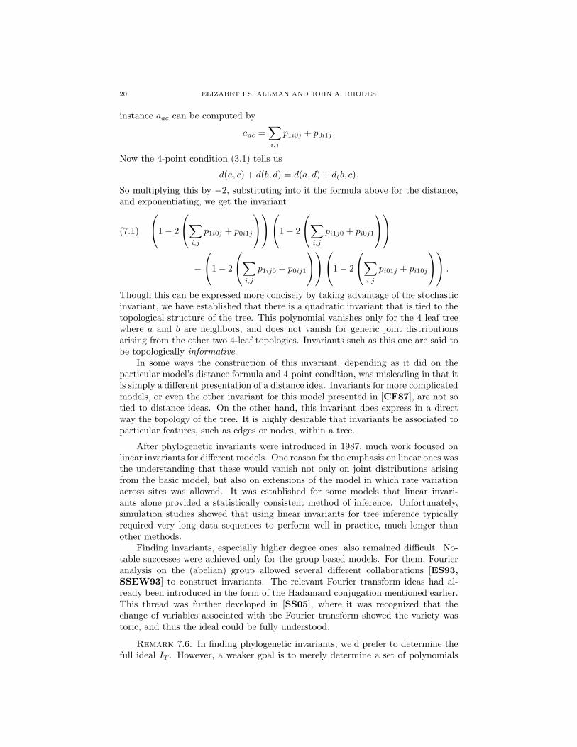
Now the 4-point condition (3.1) tells us

d(a, c) + d(b, d) = d(a, d) + d(b, c).

So multiplying this by −2, substituting into it the formula above for the distance,and exponentiating, we get the invariant

(7.1)

1− 2

∑

i,j

p1i0j + p0i1j

1− 2

∑

i,j

pi1j0 + pi0j1

−1− 2

∑

i,j

p1ij0 + p0ij1

1− 2

∑

i,j

pi01j + pi10j

.

Though this can be expressed more concisely by taking advantage of the stochasticinvariant, we have established that there is a quadratic invariant that is tied to thetopological structure of the tree. This polynomial vanishes only for the 4 leaf treewhere a and b are neighbors, and does not vanish for generic joint distributionsarising from the other two 4-leaf topologies. Invariants such as this one are said tobe topologically informative.

In some ways the construction of this invariant, depending as it did on theparticular model’s distance formula and 4-point condition, was misleading in that itis simply a different presentation of a distance idea. Invariants for more complicatedmodels, or even the other invariant for this model presented in [CF87], are not sotied to distance ideas. On the other hand, this invariant does express in a directway the topology of the tree. It is highly desirable that invariants be associated toparticular features, such as edges or nodes, within a tree.

After phylogenetic invariants were introduced in 1987, much work focused onlinear invariants for different models. One reason for the emphasis on linear ones wasthe understanding that these would vanish not only on joint distributions arisingfrom the basic model, but also on extensions of the model in which rate variationacross sites was allowed. It was established for some models that linear invari-ants alone provided a statistically consistent method of inference. Unfortunately,simulation studies showed that using linear invariants for tree inference typicallyrequired very long data sequences to perform well in practice, much longer thanother methods.

Finding invariants, especially higher degree ones, also remained difficult. No-table successes were achieved only for the group-based models. For them, Fourieranalysis on the (abelian) group allowed several different collaborations [ES93,SSEW93] to construct invariants. The relevant Fourier transform ideas had al-ready been introduced in the form of the Hadamard conjugation mentioned earlier.This thread was further developed in [SS05], where it was recognized that thechange of variables associated with the Fourier transform showed the variety wastoric, and thus the ideal could be fully understood.

Remark 7.6. In finding phylogenetic invariants, we’d prefer to determine thefull ideal IT . However, a weaker goal is to merely determine a set of polynomials

PHYLOGENETICS 21

whose zero set is VT . That is, we might be able to find a set-theoretic definition ofthe variety without determining a scheme-theoretic definition. Set-theoretic defin-ing polynomials generate an ideal whose radical is the full ideal, but determiningthat radical may be difficult.

The GM Model. In the setting of the GM model, when κ = 2 all invariantscan be understood as arising from topological features of a tree T , and for largerκ that is at least conjecturally true. We will outline some of the results from[AR05a] to elaborate on these claims. Note that many of the other models wehave mentioned are submodels of the GM model, and so invariants for GM are alsoinvariants for them.

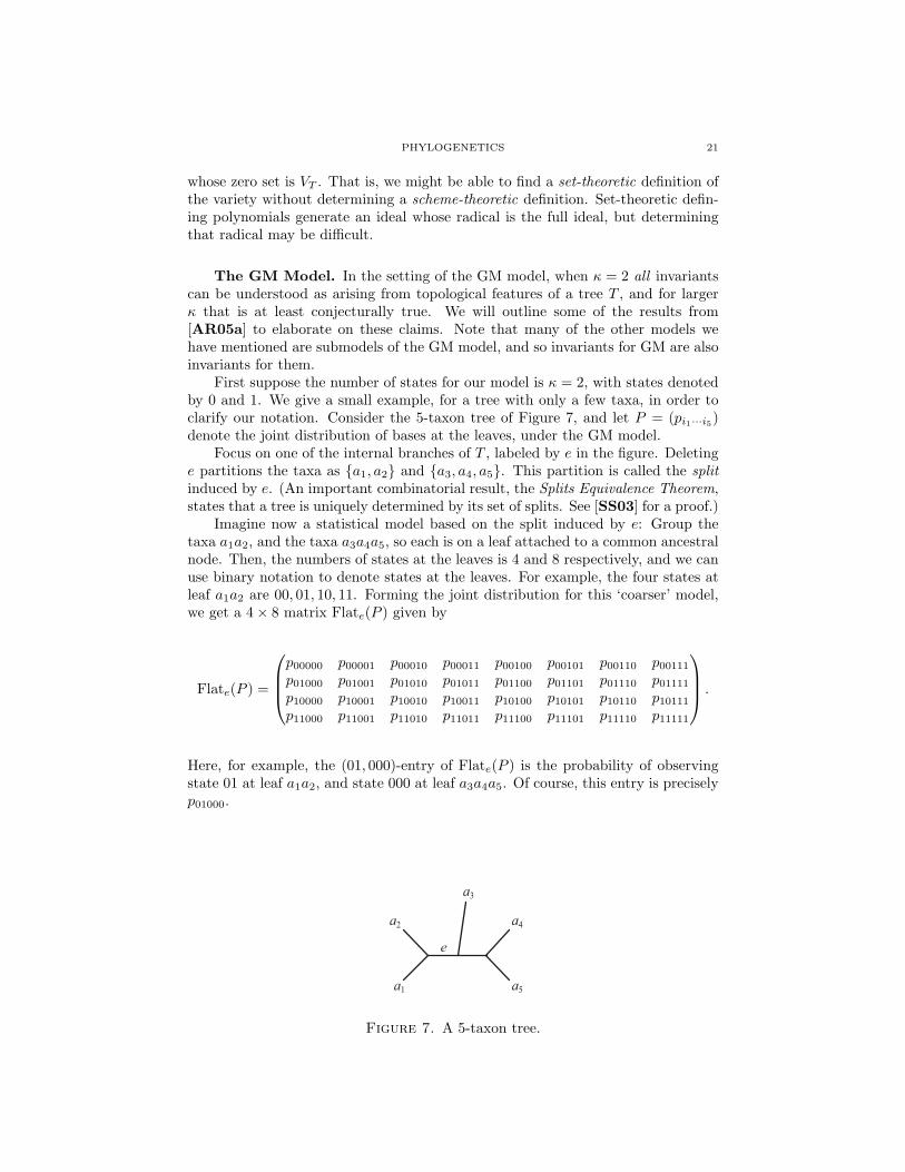
First suppose the number of states for our model is κ = 2, with states denotedby 0 and 1. We give a small example, for a tree with only a few taxa, in order toclarify our notation. Consider the 5-taxon tree of Figure 7, and let P = (pi1···i5)denote the joint distribution of bases at the leaves, under the GM model.

Focus on one of the internal branches of T , labeled by e in the figure. Deletinge partitions the taxa as {a1, a2} and {a3, a4, a5}. This partition is called the splitinduced by e. (An important combinatorial result, the Splits Equivalence Theorem,states that a tree is uniquely determined by its set of splits. See [SS03] for a proof.)

Imagine now a statistical model based on the split induced by e: Group thetaxa a1a2, and the taxa a3a4a5, so each is on a leaf attached to a common ancestralnode. Then, the numbers of states at the leaves is 4 and 8 respectively, and we canuse binary notation to denote states at the leaves. For example, the four states atleaf a1a2 are 00, 01, 10, 11. Forming the joint distribution for this ‘coarser’ model,we get a 4× 8 matrix Flate(P ) given by

Flate(P ) =

p00000 p00001 p00010 p00011 p00100 p00101 p00110 p00111

p01000 p01001 p01010 p01011 p01100 p01101 p01110 p01111

p10000 p10001 p10010 p10011 p10100 p10101 p10110 p10111

p11000 p11001 p11010 p11011 p11100 p11101 p11110 p11111

.

Here, for example, the (01, 000)-entry of Flate(P ) is the probability of observingstate 01 at leaf a1a2, and state 000 at leaf a3a4a5. Of course, this entry is preciselyp01000.

e

a1

a2

a5

a3

a4

Figure 7. A 5-taxon tree.

22 ELIZABETH S. ALLMAN AND JOHN A. RHODES

The other internal edge of T similarly induces the split {{a1, a2, a3}, {a4, a5}}and a ‘coarser’ model with joint distribution given by the 8× 4 matrix

Flate2(P ) =

p00000 p00001 p00010 p00011

p00100 p00101 p00110 p00111

p01000 p01001 p01010 p01011

p01100 p01101 p01110 p01111

p10000 p10001 p10010 p10011

p10100 p10101 p10110 p10111

p11000 p11001 p11010 p11011

p11100 p11101 p11110 p11111

.

Here the rows are indexed by the states at a1a2a3 and columns by the states ata4a5.

Each of the two matrices above are simply rearrangements of the entries of the5-dimensional tensor P into 2-dimensional arrays. Each such flattening is associatedwith a split, or internal edge, of T .

From these examples, it should be clear that for an n-leaf tree, where P isn-dimensional, we can similarly define the matrices Flate(P ), where e is any edgeof the tree.

Theorem 7.7. [AR05a] For the GM model with κ = 2 states on an n-leaf treeT , the phylogenetic ideal IT is generated by all 3 × 3 minors of Flate(P ) for alledges e of T .

In the specific case of the 5-taxon tree of Figure 7, the theorem says all 3 × 3minors of the two matrices above generate IT . We need not bother with flatteningsalong pendant edges, since they have no 3× 3 minors.

Notice especially that Theorem 7.7 is a scheme-theoretic statement; it saysthat all phylogenetic invariants are generated by the minors. Moreover, it relatestopological features of T (edges e) to invariants (minors).

It is worthwhile to outline some ideas that arise in the proof Theorem 7.7, togain more insight into how this result might be generalized to κ > 2 , and into thespecial circumstances for κ = 2 that allow us to obtain a scheme-theoretic result.

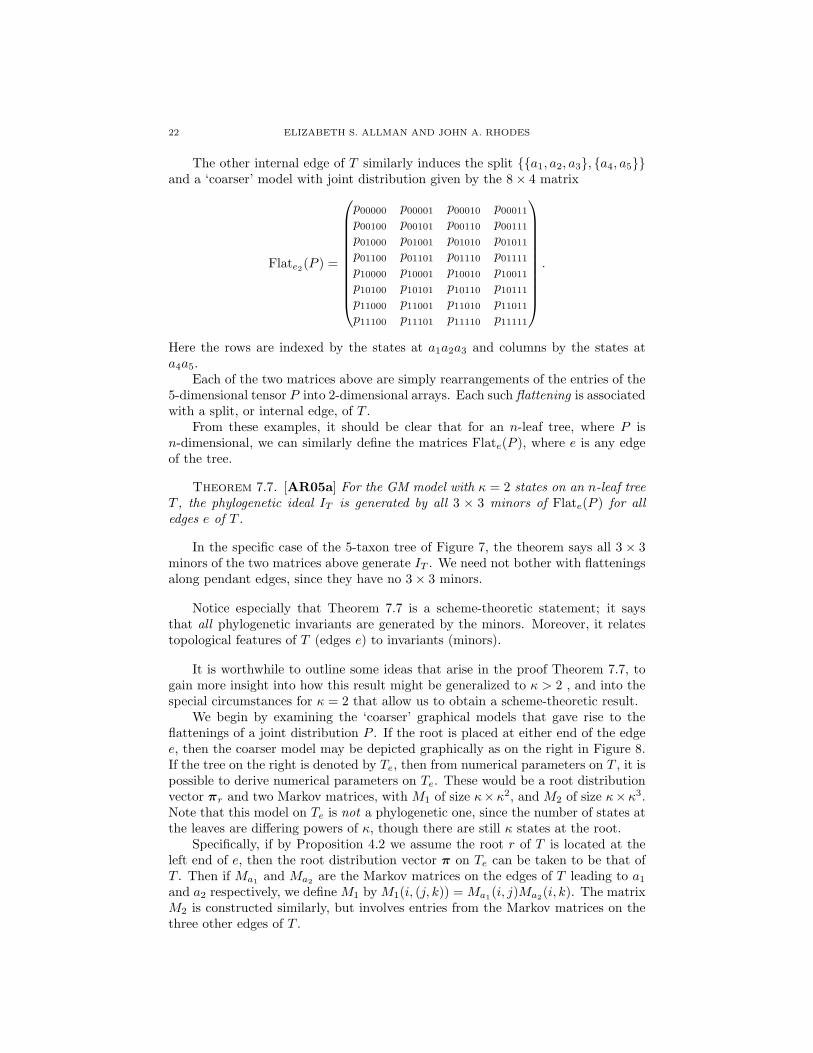
We begin by examining the ‘coarser’ graphical models that gave rise to theflattenings of a joint distribution P . If the root is placed at either end of the edgee, then the coarser model may be depicted graphically as on the right in Figure 8.If the tree on the right is denoted by Te, then from numerical parameters on T , it ispossible to derive numerical parameters on Te. These would be a root distributionvector πr and two Markov matrices, with M1 of size κ×κ2, and M2 of size κ×κ3.Note that this model on Te is not a phylogenetic one, since the number of states atthe leaves are differing powers of κ, though there are still κ states at the root.

Specifically, if by Proposition 4.2 we assume the root r of T is located at theleft end of e, then the root distribution vector π on Te can be taken to be that ofT . Then if Ma1 and Ma2 are the Markov matrices on the edges of T leading to a1

and a2 respectively, we define M1 by M1(i, (j, k)) = Ma1(i, j)Ma2(i, k). The matrixM2 is constructed similarly, but involves entries from the Markov matrices on thethree other edges of T .

PHYLOGENETICS 23

r

M1 M2e

κ3

{

κ2

}a1

a2

a3

a1a2

a4

a5a3a4a5

Figure 8. A graphical model giving rise to edge invariants.

The relationship between the joint distribution Flate(P ) for the coarser modelon Te and its numerical parameters is now expressed as:

(7.2) Flate(P ) = MT1 diag (π)M2.

Exercise 7.8. Verify Equation (7.2).

Equation (7.2) immediately reveals why phylogenetic invariants arising fromedge flattenings must exist for any tree T and any number of states κ. Since thediagonal matrix diag (π) is of size κ× κ, Flate(P ) must have rank ≤ κ. The edgeinvariants, (κ + 1)× (κ + 1)-minors from flattenings along edges, are phylogeneticinvariants indicating that Flate(P ) satisfies the given rank condition.

Remark 7.9. The well-known fact that the vanishing of all (k + 1) × (k + 1)minors of a matrix implies its rank is at most k ensures these minors are in theideal defining the variety of rank ≤ k matrices. In fact, these minors generate thatideal.

Definition 7.10. Suppose T is an n-taxon tree with κ states at each node,and P a joint distribution of states at the leaves of T arising from the GM modelon T , or any submodel of the GM model. Let Flate(P ) denote the flattening ofP induced by an edge e of T . Then the collection of (κ + 1) × (κ + 1)-minors ofFlate(P ) is the set of edge invariants for e. The set of edge invariants of T is theunion of the sets of edge invariants for all edges of T .

We therefore have shown

Proposition 7.11. For any κ, the κ-state GM model on T , or any submodel,the phylogenetic ideal contains all edge invariants.

Theorem 7.7 thus claims that edge invariants are essentially the only invariantsfor GM when κ = 2. This was conjectured in [PS04b].

Though the construction of edge invariants is natural from the viewpoint ofstatistical models, the proof of Theorem 7.7 involves different sorts of mathematicalideas: a special fact about a certain Segre variety when κ = 2, group actions ofGL(2) and GL(4) on varieties, and some representation theory.

To hint at this material, we explain a connection between the κ-state GM modelon a 3-leaf tree and a classical object in algebraic geometry. More details can befound in [GSS05, AR05a].

24 ELIZABETH S. ALLMAN AND JOHN A. RHODES

f

a1

a2

a3

Figure 9. The 3-taxon tree.

In Section 4, when stochastic models of the base substitution process wereintroduced, we assumed that the root distribution vectors and rows of the Markovmatrices sum to 1. Indeed, the probabilistic interpretation of our model requiredthat. However, from a viewpoint of algebraic geometry, these conditions simply saythe row vectors are chosen from a certain affine subset of a projective space. If weuse projective coordinates, so vectors are determined only up to scalar multiples,we view each row of the Markov matrices as an element of Pκ−1.

At the same time, we should view VT projectively. The stochastic invariant,which states that the entries of P ∈ VT add to 1, tells us VT actually lies in an affinesubset of Pκn−1. A projective viewpoint means we drop the stochastic invariant,and look for generators of a homogeneous ideal of phylogenetic invariants.

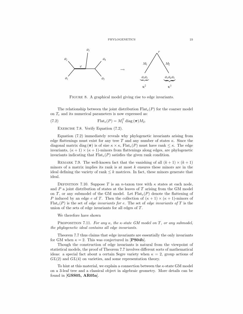
Consider then the 3-taxon tree T3 of Figure 9 in the projective setting for κstates. Fix the root at the internal node f of T3 and suppose, momentarily, thatthe state at the root is fixed as l. Then for each edge leading away from f , towardstaxon ai, we have a point vlai ∈ Pκ−1 that represents the lth row of a Markovmatrix. The entries of vlai = (vl1, · · · , vlj , · · · , vlκ) denote, up to a scaling factor,the probability that state l at f becomes state j at ai.

Thus, if we form

P l = vla1 ⊗ vla2 ⊗ vla3 ∈ Pκ−1 × Pκ−1 × Pκ−1,

then P l is a point in the Segre product of three projective spaces whose entries (upto scaling) are the expected frequency of observing pattern ijk conditioned on thestate at the internal node f being l.

Summing over all possible states at f , we obtain the joint distribution P is

P = P 1 + P 2 + · · ·+ Pκ.

(While not explicitly appearing, the root distribution has been accounted for inthe arbitrary scaling factors that appear in each P l when we choose particularprojective coordinates to express them.) Now just as sums of two points on aprojective variety gives points on secant lines to the variety, the (closure of the)union of which is the secant variety, we can consider higher secant varieties as well.Since we are summing κ points on the variety Pκ−1 × Pκ−1 × Pκ−1, we obtain

P ∈ VT3 = Secκ(Pκ−1 × Pκ−1 × Pκ−1),

the κ-secant variety of the Segre product of three Pκ−1.

More concretely, the joint distribution P has been decomposed as the sum of κrank 1 tensors, one for each possible state at the internal node f . This is preciselythe definition that P has tensor rank at most κ, and we have established that thephylogenetic variety VT3 is the (closure of) the set of κ × κ × κ tensors of rank atmost κ.

PHYLOGENETICS 25

The concept of tensor rank, as the minimal number of rank 1 summands toproduce a tensor, parallels one of the many possible definitions of matrix rank. Forthose who have not run across tensor rank before, we point out it is considerablymore subtle than its matrix analogue. For instance, there is still no straightforwardway to determine the rank of an arbitrarily chosen tensor, even in the 3-dimensionalcase. Neither analogues of matrix minors, nor an algorithmic method analogous toGaussian elimination are known. However, because of the widespread appearanceof the concept in applications, there are approaches to finding decompositions assums of rank 1 tensors, though not necessarily minimal ones.

When κ = 2, however, things are simple. Indeed, the GM model on a 3-taxon tree has only 7 parameters, and since the stochastic invariant cuts out a7-dimensional subspace of C23

, one might conjecture there are no other invariants.In fact, this is the case, and Sec2(P1×P1×P1) = P7. In other words, every 2×2×2tensor is in the closure of the rank 2 ones. (Note this does not mean every suchtensor has rank 2.) This special fact plays an important role in [AR05a].

For κ = 3, the ideal defining Secκ(Pκ−1×Pκ−1×Pκ−1) was found in [GSS05],using results from [Str83]. For κ = 4, polynomials are known that generate theideal only up to saturation with respect to another explicitly given variety, and thentaking a radical [AR03]. In this case there are 1728 independent quintics, whichare known to be all such quintics. See [Hag00] for computation of this dimension,or [LM04] for a broader set of computations of dimensions of spaces of polynomialsvanishing on various secant varieties of Segre varieties.

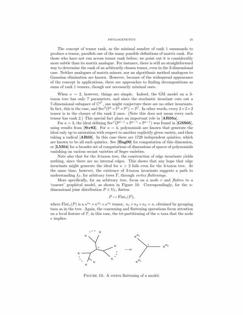
Note also that for the 3-taxon tree, the construction of edge invariants yieldsnothing, since there are no internal edges. This shows that any hope that edgeinvariants might generate the ideal for κ > 2 fails even for the 3-taxon tree. Atthe same time, however, the existence of 3-taxon invariants suggests a path tounderstanding IT , for arbitrary trees T , through vertex flattenings.

More specifically, for an arbitrary tree, focus on a node v and flatten to a‘coarser’ graphical model, as shown in Figure 10. Correspondingly, for the n-dimensional joint distribution P ∈ VT , flatten

P 7→ Flatv(P ),

where Flatv(P ) is a κn1×κn2×κn3 tensor, n1 +n2 +n3 = n, obtained by groupingtaxa as in the tree. Again, the coarsening and flattening operations focus attentionon a local feature of T , in this case, the tri-partitioning of the n taxa that the nodev implies.

vv

κ

κ

κκ

κ

κn1

κn3

κn2

κ

κ

Figure 10. A vertex flattening of a model.

26 ELIZABETH S. ALLMAN AND JOHN A. RHODES

κ

l1

l2

l3κ

κκ

l1

l2

l3

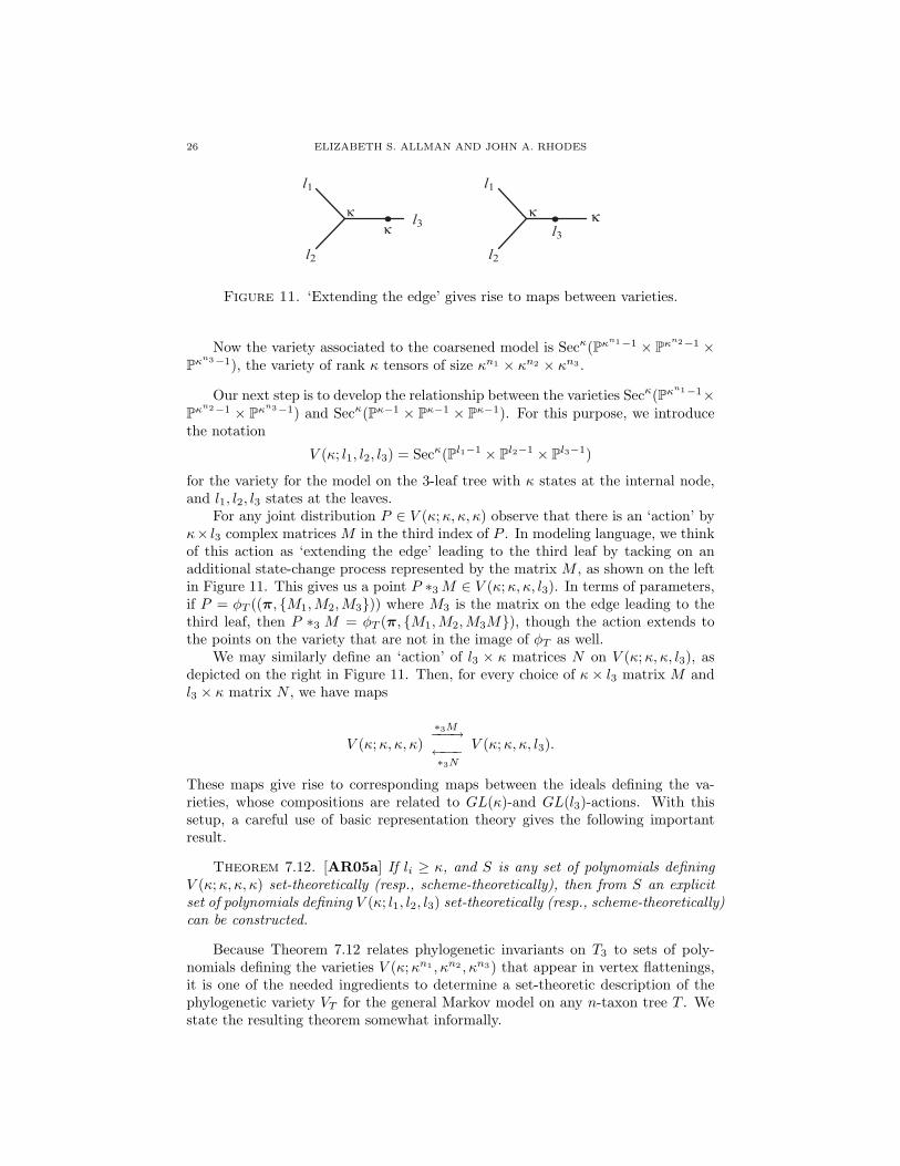
Figure 11. ‘Extending the edge’ gives rise to maps between varieties.

Now the variety associated to the coarsened model is Secκ(Pκn1−1 × Pκn2−1 ×Pκn3−1), the variety of rank κ tensors of size κn1 × κn2 × κn3 .

Our next step is to develop the relationship between the varieties Secκ(Pκn1−1×Pκn2−1 × Pκn3−1) and Secκ(Pκ−1 × Pκ−1 × Pκ−1). For this purpose, we introducethe notation

V (κ; l1, l2, l3) = Secκ(Pl1−1 × Pl2−1 × Pl3−1)

for the variety for the model on the 3-leaf tree with κ states at the internal node,and l1, l2, l3 states at the leaves.

For any joint distribution P ∈ V (κ; κ, κ, κ) observe that there is an ‘action’ byκ× l3 complex matrices M in the third index of P . In modeling language, we thinkof this action as ‘extending the edge’ leading to the third leaf by tacking on anadditional state-change process represented by the matrix M , as shown on the leftin Figure 11. This gives us a point P ∗3 M ∈ V (κ; κ, κ, l3). In terms of parameters,if P = φT ((π, {M1, M2,M3})) where M3 is the matrix on the edge leading to thethird leaf, then P ∗3 M = φT (π, {M1,M2,M3M}), though the action extends tothe points on the variety that are not in the image of φT as well.

We may similarly define an ‘action’ of l3 × κ matrices N on V (κ; κ, κ, l3), asdepicted on the right in Figure 11. Then, for every choice of κ× l3 matrix M andl3 × κ matrix N , we have maps

V (κ; κ, κ, κ)∗3M−−−→←−−−∗3N

V (κ;κ, κ, l3).

These maps give rise to corresponding maps between the ideals defining the va-rieties, whose compositions are related to GL(κ)-and GL(l3)-actions. With thissetup, a careful use of basic representation theory gives the following importantresult.

Theorem 7.12. [AR05a] If li ≥ κ, and S is any set of polynomials definingV (κ; κ, κ, κ) set-theoretically (resp., scheme-theoretically), then from S an explicitset of polynomials defining V (κ; l1, l2, l3) set-theoretically (resp., scheme-theoretically)can be constructed.

Because Theorem 7.12 relates phylogenetic invariants on T3 to sets of poly-nomials defining the varieties V (κ;κn1 , κn2 , κn3) that appear in vertex flattenings,it is one of the needed ingredients to determine a set-theoretic description of thephylogenetic variety VT for the general Markov model on any n-taxon tree T . Westate the resulting theorem somewhat informally.

PHYLOGENETICS 27

Theorem 7.13. [AR05a] For the 3-taxon tree T3, let S be a set of polynomi-als defining V (κ; κ, κ, κ) set-theoretically. Then, using vertex flattenings and theconstruction of Theorem 7.12, for an arbitrary binary tree T a set of polynomialsset-theoretically defining VT for the general Markov model can be explicitly given.

An important consequence of Theorem 7.13 is that phylogenetic invariants forthe general Markov model are intimately related to the nodes and edges of T . Thelocal structure of a tree determines a collection of phylogenetic invariants definingthe variety VT . Note that (using different techniques) this sort of result for group-based models had already been established in [SS05]. Possible ways this might beuseful will be discussed in the next section.

8. Potential uses of invariants

So far, invariants have not planned a large role in practical inference by biol-ogists. However, now that we are beginning to understand them better, that maywell change. In this section we outline some of the ideas now under development.

Tree-building heuristics. A key property of the invariants we understand isthat specific polynomials can be tied to local structure of a tree (edges or nodes).They might therefore be used to develop tests for only such local structures, withoutconsideration of the entire tree.

To elaborate, one inherent feature of maximum likelihood is that it not onlychooses the ‘best’ tree, but also ‘best’ values for all parameters. This is preciselywhy ML inference can be such a large computational problem; it looks at every-thing at once. However, for building a tree from data (and for some biologicalquestions) we might first look for strongly-supported splits of our taxa (in bio-logical terminology, for monophyletic clades). If specific invariants can be tied toedges (splits) and nodes (tripartitions), perhaps we can address the support foreach feature individually.

One step toward using this viewpoint to infer trees has been taken in [Eri05].There an algorithm is given for building trees that is reminiscent of Neighbor Join-ing in its ‘outside-first’ iterative approach. The scheme for joining taxa, though,is based on edge invariants. Rather than evaluate polynomials, however, the sin-gular value decomposition of matrices is used to determine approximate matrixrank. Preliminary results on the algorithm’s performance were reported as posi-tive, though not as strong as more standard methods. Nonetheless, the comparisonswere probably biased against the new method, since data was simulated accordingto much simpler model than GM, that, among other things, assumes the same dis-tribution of bases in all sequences. We believe that there is much room for furtherdevelopment along these lines.

Even if we prefer to stick with a full maximum likelihood framework for in-ference, we must acknowledge that implementations in software require heuristicsearches if more than a handful of taxa are involved. For the numerical parameters,optimization is a well-studied problem and we might assume this part of the searchcan be done adequately. For the tree parameter, though, how should we vary thetree in order to increase likelihoods? Perhaps invariants can be used to identifymore weakly supported edges or nodes in the tree which should be removed in re-configuring. If they are effective at suggesting how we might move toward optimain tree-space, they may help speed up searches.

28 ELIZABETH S. ALLMAN AND JOHN A. RHODES

Exact solutions of ML problems. Since for large problems, ML inferencemust be done heuristically, it would be desirable to understand better under whatcircumstances there might be one, or more, global optimum, and whether we havemany local optima. Invariants have placed a role in studying these questions,by allowing ML estimation to be phrased as a constrained optimization problem,with invariants providing the constraints. See [CHHP00, CHP01, CKS03] forsome examples of this sort of work. [HKS05] provides a more general setting forcomputational algebra approaches to ML, as well as phylogenetic examples.

The “Small Trees website’ [CGS05] is a good resource allowing an easy inter-face from trees and models to computational algebra package formulations. Finally[CL05] suggests how solving ML problems well on small trees can, with a general-ized Neighbor Joining approach, lead to construction of large trees.

Identifiability of tree topologies for models. An important issue in deal-ing with any statistical model is identifiability : Given a joint distribution arisingfrom the model, is it possible to recover the parameters leading to the distribution?Clearly, identifiability of any parameters of interest is a necessary condition to ourestimating them well. Indeed, proofs of the statistical consistency of ML begin withproofs of identifiability.

Identifiability has been established for many phylogenetic models routinely used(for instance, GTR+I+Γ; GM, and hence any submodel of GM). Provided a dis-tance can be defined for the model, the 4-point condition can be used to identifytopologies. In fact, since distances require comparing only two sequences at a time(i.e., are based on 2-dimensional marginalizations of the joint distribution P ), iden-tifying the tree does not even require the full joint distribution. On the other hand,[Baa98] established that the tree could not be identified by 2-sequence compar-isons for the model GM+I. In general, identifiability for mixture models of this sorthas been poorly understood. Even for GTR+(rate distribution), proofs of identi-fiability of the tree require that the rate distribution be known. See [SSH94] and[BGP05].

Recently some specific invariants that have not been discussed here have beenused to obtain some general results on identifiability of tree topologies. In [AR05b]it is shown that for a mixture model where the number of classes is less thanthe number of states (e.g., at most 3 classes for a 4-state model for DNA), treetopology is identifiable for generic choices of parameters. This result makes noassumptions of any commonality to the substitution process among the differentclasses; they need not be based on any common rate matrix. The result also appliesto a covarion model [TS98] in which sites in a sequence may only be free to varyin some (unknown) parts of the tree, switching between variable and invariable andback as evolution proceeds over the tree

To prove such identifiability results, an algebraic mutation model is introducedwhich allows more states at internal nodes of the tree than at the leaves. In this verygeneral setting, it is possible to show that parameters are generically identifiable,and then to argue that each of the models listed above is a specialization of thismodel, and that generic identifiability is maintained after specialization. The keysteps in the proof involve finding invariants that express appropriate rank conditionssimilar to those that arose in the edge flattenings and vertex flattenings of Theorems7.7 and 7.13.

PHYLOGENETICS 29

9. Further Reading and Software Packages

For mathematicians interested in learning more about phylogenetics, we suggesta few books. Felsenstein’s book [Fel04], written for a diverse audience, is the mostcomplete survey of the field, with many references. The text [SS03] by Semple andSteel is more mathematical, emphasizing the combinatorial aspects. Pachter andSturmfels, in [PS05], provide an excellent introduction to the algebraic viewpoint.The volume [Gas05] provides a collection of articles on many more aspects ofphylogenetics than we have been able to even touch on here.

For undergraduate teaching, the only presentation we know of any material onthe mathematics behind phylogenetics appears in [AR04].

There are many software packages used by biologists for phylogenetic inference.PHYLIP, which is freely available over the web from the Felsenstein lab is a goodcollection of programs to begin exploring. Most published biological papers willindicate what software was used for inference, so finding pointers to other packagesis relatively easy.

References

[AR03] Elizabeth S. Allman and John A. Rhodes. Phylogenetic invariants for the generalMarkov model of sequence mutation. Math. Biosci., 186:113–144, 2003.

[AR04] Elizabeth S. Allman and John A. Rhodes. Mathematical Models in Biology: an Intro-duction. Cambridge University Press, 2004.

[AR05a] Elizabeth S. Allman and John A. Rhodes. Phylogenetic ideals and varieties for thegeneral Markov model. 2005. preprint, arXiv:math.AG/0410604.

[AR05b] Elizabeth S. Allman and John A. Rhodes. The identifiability of tree topologyfor phylogenetic models, including covarion and mixture models. 2005. preprint,q-bio.PE/0511009.

[AR06] Elizabeth S. Allman and John A. Rhodes. Phylogenetic invariants for stationary basecomposition. J. Symbolic Comp., 41(2):138–150, 2006.

[Baa98] Ellen Baake. What can and what cannot be inferred from pairwise sequence compar-isons? Math. Biosci., 154(1):1–21, 1998.

[BGP05] David Bryant, Nicolas Galtier, and Marie-Anne Poursat. Likelihood caclulation inmolecular phylogenetics. In Olivier Gascuel, editor, Mathematics of Evolution andPhylogeny, pages 33–62. Oxford University Press, 2005.

[Bun71] Peter Buneman. The recovery of trees from measures of dissimilarity. In Mathematics inthe Archeological and Historical Sciences, pages 387–395, Edinburgh, 1971. EdinburghUniversity Press.

[CF87] James A. Cavender and Joseph Felsenstein. Invariants of phylogenies in a simple casewith discrete states. J. of Class., 4:57–71, 1987.

[CGS05] Marta Casanellas, Luis David Garcia, and Seth Sullivant. Catalog of smalltrees. In Lior Pachter and Bernd Sturmfels, editors, Algebraic Statisticsfor Computational Biology, pages 291–304. Cambridge University Press, 2005.http://www.math.tamu.edu/~ lgp/small-trees/.

[CHHP00] B. Chor, M. D. Hendy, B. R. Holland, and D. Penny. Multiple maxima of likelihoodin phylogenetic trees: an analytic approach. Mol. Bio. and Evol., 17:1529–1541, 2000.

[CHP01] Benny Chor, Michael Hendy, and David Penny. Analytic solutions for three-taxonMLMC trees with variable rates across sites. In Algorithms in bioinformatics (Arhus,2001), volume 2149 of Lecture Notes in Comput. Sci., pages 204–213. Springer, Berlin,2001.

[CKS03] B. Chor, A. Khetan, and S. Snir. Maximum likelihood on four taxa phylogenetic trees:Analytic solutions. RECOMB’03, 2003.

[CL05] Mark Contois and Dan Levy. Small trees and generalized neighbor-joining. In LiorPachter and Bernd Sturmfels, editors, Algebraic Statistics for Computational Biology,pages 335–346. Cambridge University Press, 2005.

30 ELIZABETH S. ALLMAN AND JOHN A. RHODES

[CLO97] David Cox, John Little, and Donal O’Shea. Ideals, varieties, and algorithms. Springer-Verlag, New York, second edition, 1997.

[Eri05] Nicholas Eriksson. Tree construction using singular value decomposition. In LiorPachter and Bernd Sturmfels, editors, Algebraic Statistics for Computational Biol-ogy, pages 347–358. Cambridge University Press, 2005.

[ES93] Steven N. Evans and T. P. Speed. Invariants of some probability models used in phy-logenetic inference. Ann. Statist., 21(1):355–377, 1993.

[Fel78] J. Felsenstein. Cases in which parsimony or compatibility methods will be positivelymisleading. Systematic Zoology, 27:401–410, 1978.

[Fel04] Joseph Felsenstein. Inferring Phylogenies. Sinauer Associates, Sunderland, MA, 2004.[FG82] L. R. Foulds and R. L. Graham. The Steiner problem in phylogeny is NP-complete.

Adv. in Appl. Math., 3(1):43–49, 1982.[Gas05] Olivier Gascuel, editor. Mathematics of Evolution and Phylogeny. Oxford University

Press, Oxford, 2005.[GPS01] G.-M. Greuel, G. Pfister, and H. Schonemann. Singular 2.0. A Computer Algebra

System for Polynomial Computations, Centre for Computer Algebra, University ofKaiserslautern, 2001. http://www.singular.uni-kl.de.

[GS02] Daniel R. Grayson and Michael E. Stillman. Macaulay2, a software system for researchin algebraic geometry. Available at http://www.math.uiuc.edu/Macaulay2/, 2002.

[GSS05] Luis David Garcia, Michael Stillman, and Bernd Sturmfels. Algebraic geometry ofBayesian networks. J. Symbolic Comp., 39:331–355, 2005. arXiv:math.AG/0301255.

[Hag00] Thomas R. Hagedorn. A combinatorial approach to determining phylogenetic invari-ants for the general model, 2000. Technical report, Centre de recherches mathmatiques.

[Hen89] Michael D. Hendy. The relationship between simple evolutionary tree models and ob-servable sequence data. Systematic Zoology, 38:310–321, 1989.

[HGH88] K. Hayasaka, T. Gojobori, and S. Horai. Molecular phylogeny and evolution of primatemitochondrial DNA. Mol. Biol. Evol., 5:626–644, 1988.

[HKS05] Serkan Hosten, Amit Khetan, and Bernd Sturmfels. Solving the Likelihood Equations.Found. Comput. Math., 2005. to appear, arXiv:math.ST/0408270.

[HP89] Michael D. Hendy and David Penny. A framework for the quantitative study of evolu-tionary trees. Systematic Zoology, 38:297–309, 1989.

[Lak87] J.A. Lake. A rate independent technique for analysis of nucleic acid sequences: Evo-lutionary parsimony. Mol. Bio. Evol., 4(2):167–191, 1987.

[LM04] J. M. Landsberg and L. Manivel. On the ideals of secant varieties of Segre varieties.Found. Comput. Math., 4(4):397–422, 2004.

[PS04a] L. Pachter and D. Speyer. Reconstructing trees from subtree weights. Appl. Math.Lett., 17(6):615–621, 2004.

[PS04b] Lior Pachter and Bernd Sturmfels. Tropical geometry of statistical models. Proc. Natl.Acad. Sci. USA, 101(46):16132–16137 (electronic), 2004.

[PS05] Lior Pachter and Bernd Sturmfels, editors. Algebraic Statistics for ComputationalBiology. Cambridge University Press, Cambridge, 2005.

[SK88] J.A. Studier and K.J. Keppler. A note on the neighbor-joining algorithm of saitou andnei. Mol. Biol. Evol., 5(5):729–731, 1988.

[SN87] N. Saitou and M. Nei. The neighbor-joining method: A new method for reconstructingphylogenetic trees. Mol. Biol. Evol., 4:406–425, 1987.

[SS03] Charles Semple and Mike Steel. Phylogenetics, volume 24 of Oxford Lecture Series inMathematics and its Applications. Oxford University Press, Oxford, 2003.

[SS05] Bernd Sturmfels and Seth Sullivant. Toric ideals of phylogenetic invariants. J. Comput.Biol., 12(2):204–228, 2005. arXiv:q-bio.PE/0402015.

[SSE93] L. A. Szekely, M. A. Steel, and P. L. Erdos. Fourier calculus on evolutionary trees.Adv. in Appl. Math., 14(2):200–210, 1993.

[SSEW93] Mike Steel, Laszlo Szekely, Peter L. Erdos, and Peter Waddell. A complete family ofphylogenetic invariants for any number of taxa under Kimura’s 3ST model. N.Z. J.Botany, 31(31):289–296, 1993.

[SSH94] M.A. Steel, L. Szekely, and M.D. Hendy. Reconstructing trees from sequences whosesites evolve at variable rates. J. Comput. Biol., 1(2):153–163, 1994.

[Str83] V. Strassen. Rank and optimal computation of generic tensors. Linear Algebra Appl.,52/53:645–685, 1983.

PHYLOGENETICS 31

[TS98] Chris Tuffley and Mike Steel. Modeling the covarion hypothesis of nucleotide substi-tution. Math. Biosci., 147(1):63–91, 1998.

Department of Mathematics and Statistics, University of Alaska Fairbanks, POBox 756660, Fairbanks, Alaska 99775

E-mail address: e.allman@uaf.edu

Department of Mathematics and Statistics, University of Alaska Fairbanks, POBox 756660, Fairbanks, Alaska 99775

E-mail address: j.rhodes@uaf.edu