Embed Size (px)
Citation preview
EURECOMCampus SophiaTech
CS 5019306904 Sophia Antipolis cedex FRANCE
Research Report RR-16-317PHY and MAC layer Modeling of LTE and WiFi RATs
March 24, 2016
George Arvanitakis and Florian Kaltenberger
Tel : (+33) 4 93 00 81 00Fax : (+33) 4 93 00 82 00
Email : {George.Arvanitakis}@eurecom.fr
1EURECOM’s research is partially supported by its industrial members: BMW Group Researchand Technology, IABG, Monaco Telecom, Orange, Principaut de Monaco, SAP, SFR, ST Microelec-tronics, Symantec
1

Abstract
We consider LTE and WiFi networks in order to model both PHY and MAC
layers. Our physical layer abstraction consists a mapping between user’s SINR and
their corresponding rate. On the other hand, we will propose a proper queue model
to represent the schedulers of each radio access technique (RAT), at the MAC layer.
2
1 Introduction
The scope of this technical report is the proper modeling of both PHY and
MAC layer of two widely used radio access techniques (RATs), LTE and WiFI. So,
we have two main tasks, one for each layer (one for PHY and one for MAC).
• To match the user’s SINR with the corresponding data rate. This tasks needs
two internal steps: i) specify the SINR threshold of each MCS, ii) specify
the rate of each MCS.
• To answer, how the resources are allocated with the presence of other users,
and how the overall performance of the systems depends on the users’ rate
distribution. In other words, we should model each RAT scheduler with a
proper queueing system in order to be able to analyze the dynamic behavior
of a base station in terms of incoming load.
This work supposes 20MHz eNodeB with a single antenna and a 802.11n sin-
gle stream access point, both of them operate with 20MHz bandwidth, but easily
could be extended to other cases.
2 PHY modeling
The supported MCS modes are RAT depended and always defined at the cor-
responding protocol description documents [1], [2]. The operation threshold for
each mode is not always defined in the protocol since it heavily depends on the
receiver implementation characteristics. So, we will need one SINR table for the
LTE modes and one for the WiFi. The reference receivers of the LTE will be the
open air interface platforms. For the WiFi we used a generic SINR threshold that
is presented at [3].
2.1 LTE
From the OpenAirInterface LTE downlink simulator [4], Block Error Rate
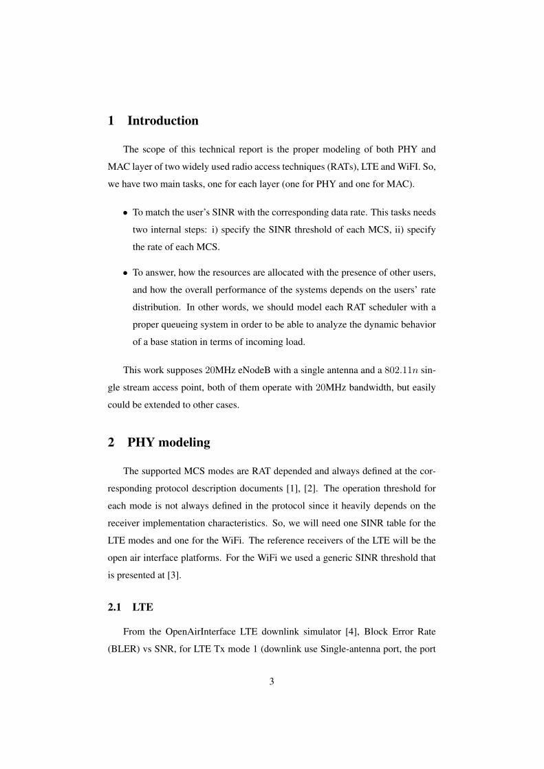
(BLER) vs SNR, for LTE Tx mode 1 (downlink use Single-antenna port, the port
3
−5 0 5 10 15 20
10−2
10−1
100
SNR
BLER
Tx mode 1: BLER vs SNR mcs 0
mcs 1
mcs 2
mcs 3
mcs 4
mcs 5
mcs 6
mcs 7
mcs 8
mcs 9
mcs 10
mcs 11
mcs 12
mcs 13
mcs 14
mcs 15
mcs 16
mcs 17
mcs 18
mcs 19
mcs 20
mcs 21
mcs 22
mcs 23
mcs 24
mcs 25
mcs 26
mcs 27
Figure 1: BLER vs SINR
0) [5], is generated for each MCS and shown in Fig. 1. So, for a given BLER
threshold (commonly at 10−1) the SINR threshold (τ ) for each MCS can be speci-
fied. Additionally, if we are interested for theoretical analysis, we can combine the
knowledge for SINR distribution (or ”coverage probability”) with MCS threshold
τ in order to end with MCS distribution.
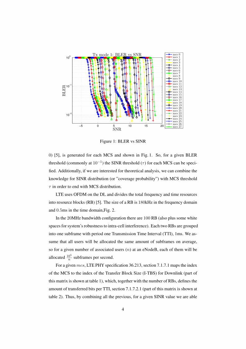
LTE uses OFDM on the DL and divides the total frequency and time resources
into resource blocks (RB) [5]. The size of a RB is 180kHz in the frequency domain
and 0.5ms in the time domain,Fig. 2.
In the 20MHz bandwidth configuration there are 100 RB (also plus some white
spaces for system’s robustness to intra-cell interference). Each two RBs are grouped
into one subframe with period one Transmission Time Interval (TTI), 1ms. We as-
sume that all users will be allocated the same amount of subframes on average,
so for a given number of associated users (n) at an eNodeB, each of them will be
allocated 105
n subframes per second.
For a givenmcs, LTE PHY specification 36.213, section 7.1.7.1 maps the index
of the MCS to the index of the Transfer Block Size (I-TBS) for Downlink (part of
this matrix is shown at table 1), which, together with the number of RBs, defines the
amount of transferred bits per TTI, section 7.1.7.2.1 (part of this matrix is shown at
table 2). Thus, by combining all the previous, for a given SINR value we are able
4
Figure 2: LTE Resource Blocks
to calculate the bit rate.
5
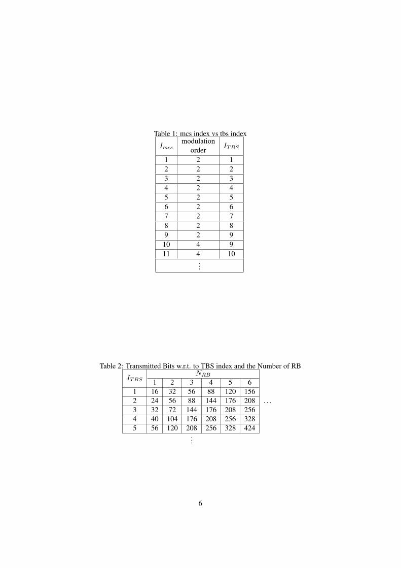
Table 1: mcs index vs tbs index
Imcsmodulation
orderITBS
1 2 12 2 23 2 34 2 45 2 56 2 67 2 78 2 89 2 9
10 4 911 4 10
...
Table 2: Transmitted Bits w.r.t. to TBS index and the Number of RB
ITBSNRB
1 2 3 4 5 61 16 32 56 88 120 1562 24 56 88 144 176 208 . . .3 32 72 144 176 208 2564 40 104 176 208 256 3285 56 120 208 256 328 424
...
6
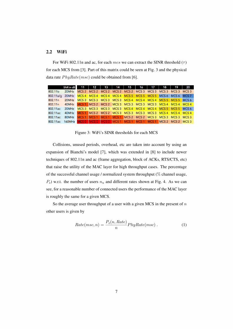
2.2 WiFi
For WiFi 802.11n and ac, for each mcs we can extract the SINR threshold (τ )
for each MCS from [3]. Part of this matrix could be seen at Fig. 3 and the physical
data rate PhyRate(msc) could be obtained from [6].
Figure 3: WiFi’s SINR thresholds for each MCS
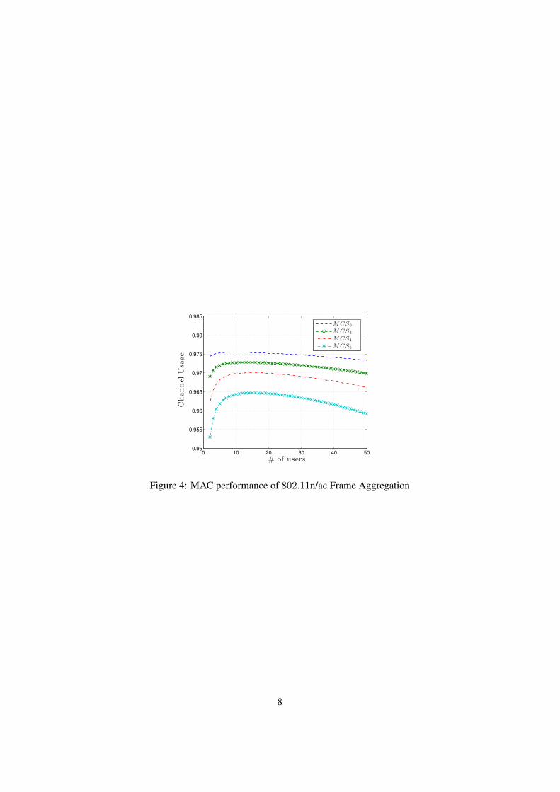
Collisions, unused periods, overhead, etc are taken into account by using an
expansion of Bianchi’s model [7], which was extended in [8] to include newer
techniques of 802.11n and ac (frame aggregation, block of ACKs, RTS/CTS, etc)
that raise the utility of the MAC layer for high throughput cases. The percentage
of the successful channel usage / normalized system throughput (% channel usage,
Ps) w.r.t. the number of users nu and different rates shown at Fig. 4. As we can
see, for a reasonable number of connected users the performance of the MAC layer
is roughly the same for a given MCS.
So the average user throughput of a user with a given MCS in the present of n
other users is given by
Rate(msc, n) =Ps(n,Rate)
nPhyRate(msc) . (1)
7
0 10 20 30 40 500.95
0.955
0.96
0.965
0.97
0.975
0.98
0.985
# of users
ChannelUsage
MCS0
MCS2
MCS4
MCS6
Figure 4: MAC performance of 802.11n/ac Frame Aggregation
8
2.3 Summary
Actual RATs do not provide an elegant way to calculate the user’s rate, so it
is common, when analyzing wireless networks to use the Shannon’s theorem, as it
constitutes a more simplified approach. When a single network is being analyzed,
this assumption does not affect the validity of the qualitative results. However,
in the case of modern heterogeneous networks (HetNets), and especially when
HetNets operate with different RAT, this assumption does not hold. The user’s rate
of different RATs does not scale with the same way, with respect to SINR.
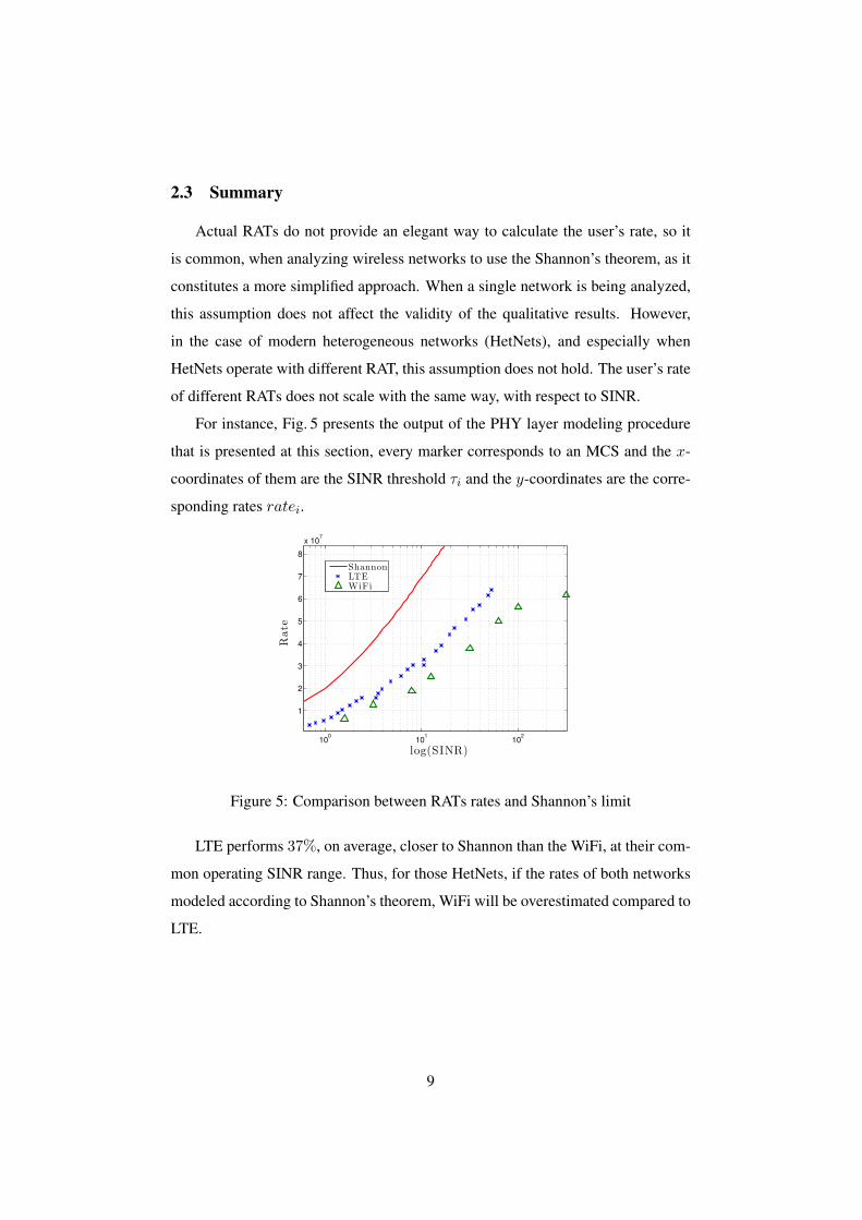
For instance, Fig. 5 presents the output of the PHY layer modeling procedure
that is presented at this section, every marker corresponds to an MCS and the x-
coordinates of them are the SINR threshold τi and the y-coordinates are the corre-
sponding rates ratei.
100
101
102
1
2
3
4
5
6
7
8
x 107
log(SINR)
Rate
ShannonLTEWiFi
Figure 5: Comparison between RATs rates and Shannon’s limit
LTE performs 37%, on average, closer to Shannon than the WiFi, at their com-
mon operating SINR range. Thus, for those HetNets, if the rates of both networks
modeled according to Shannon’s theorem, WiFi will be overestimated compared to
LTE.
9
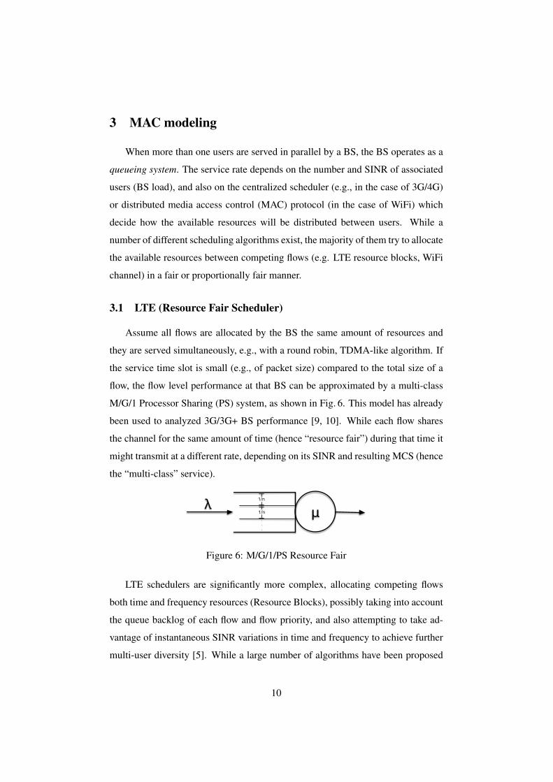
3 MAC modeling
When more than one users are served in parallel by a BS, the BS operates as a
queueing system. The service rate depends on the number and SINR of associated
users (BS load), and also on the centralized scheduler (e.g., in the case of 3G/4G)
or distributed media access control (MAC) protocol (in the case of WiFi) which
decide how the available resources will be distributed between users. While a
number of different scheduling algorithms exist, the majority of them try to allocate
the available resources between competing flows (e.g. LTE resource blocks, WiFi
channel) in a fair or proportionally fair manner.
3.1 LTE (Resource Fair Scheduler)
Assume all flows are allocated by the BS the same amount of resources and
they are served simultaneously, e.g., with a round robin, TDMA-like algorithm. If
the service time slot is small (e.g., of packet size) compared to the total size of a
flow, the flow level performance at that BS can be approximated by a multi-class
M/G/1 Processor Sharing (PS) system, as shown in Fig. 6. This model has already
been used to analyzed 3G/3G+ BS performance [9, 10]. While each flow shares
the channel for the same amount of time (hence “resource fair”) during that time it
might transmit at a different rate, depending on its SINR and resulting MCS (hence
the “multi-class” service).
μλ 1/n
1/n...
Figure 6: M/G/1/PS Resource Fair
LTE schedulers are significantly more complex, allocating competing flows
both time and frequency resources (Resource Blocks), possibly taking into account
the queue backlog of each flow and flow priority, and also attempting to take ad-
vantage of instantaneous SINR variations in time and frequency to achieve further
multi-user diversity [5]. While a large number of algorithms have been proposed
10
(see e.g., [11] for an extensive survey), in the lack of special priority traffic, most
implemented schedulers lead to a proportionally fair throughput allocation between
flows [5] and can also be approximated by a similar multi-class M/G/1 PS queue.
The following is a direct application of the multi-class M/G/1/PS result [12].
lemma: For a BS with n users generating flows of mean size 〈s〉, with instan-
taneous transmission rates drawn from distribution fR(r), and allocated resources
by a resource fair scheduler, the effective service rate of the cell is
〈µ〉rf =
(∑r
fR(r) · 〈s〉r
)−1flows/sec, (2)
and the mean flow delay is given by
E[T ]rf =1
〈µ〉rf − nλf, (3)
when the system is stable (nλf < 〈µ〉)
We further define the BS’s load as ρ = input job rateservice job rate =
nλf〈µ〉 when the system is
stable ρ < 1 .
Performance gains from opportunistic scheduling can be included in the above
equation as a multiplicative factor in front of 〈µ〉.
3.2 WiFi (Throughput Fair Scheduler)
Some schedulers attempt to achieve fairness more aggressively, by trying to
equalize per flow throughput for all nodes. For example, if two concurrent flows
experience different channel conditions (say one being “far” and one being “near”
the BS) a throughput fair scheduler will attempt to give more resources to the
flow with the worse channel (e.g., more resource blocks in the case of LTE, or
schedule the far flow more often in the case of 3G). This can be seen as a Gen-
eralized or Discriminatory Processor Sharing system (a generalized version of the
M/G/1/PS) [13], with different weights per flow that, for throughput-fair systems,
can be taken as inversely proportional to the average rate experienced by that flow.
It is known that throughput fair schedulers perform poorly compared to propor-
11
tionally fair ones, and thus are not often considered [14]. Nevertheless, throughput
fair scheduling turns out to be a good approximation of how the 802.11 WiFi MAC
allocates resources between flows [15]. In WiFi, all nodes compete for the chan-
nel and when they do get access, in the basic implementation, they send a single
frame and then have to retry. WiFi like LTE supports rate adaptation, therefore
each frame might be transmitted at a different rate, depending on the maximum
MCS that can be offered to the respective node. Nevertheless, due to the random
access MAC, each node gets access with equal chance, regardless of their distance
from the AP. If each flow corresponds to a large number of frames (usually a good
assumption given the small max size of a frame), this essentially equalizes the
long-term throughput of each flow, regardless of its MCS. Hence, the WiFi sched-
uler for a single BS could be seen as throughput-fair, and can be modeled as a
Discriminatory Processor Sharing (DPS) queue. The following lemma derives the
mean service rate (µ) for such a throughput-fair scheduler in a system with rate
adaptation.
Lemma: The mean service rate for a throughput fair scheduler with rate adap-
tation, where a random user/frame is transmitted with an instantaneous rate r with
probability fR(r), is given by
〈µ〉tf =
(∑r
fR(r) · 〈s〉r
)−1. (4)
Proof: Consider a long time interval during which N packets get transmitted, cor-
responding to different flows. Assume each packet is of equal size S (e.g., the
max WiFi frame size) but is transmitted with a possibly different rate r drawn from
pmf fR(r) with K discrete values, depending on the MCS used for transmitting
that packet. Assume that out of these N packets, Ni are transmitted with rate ri,
(∑
iNi = N ). Hence, the average transmission rate in terms of bits/sec for these
N packets is
bits in N pktstransmission time for N pkts
=N · S
N1Sr1
+N2Sr2
+ · · ·+NKSrK
(5)
12
However, as N goes to infinity, the Ni converges to its mean value fR(ri) · N by
the law of large numbers, hence the denominator of Eq.(5) converges to
limN→∞
(N1S
r1+N2
S
r2+ · · ·+NK
S
rK) =
∑fR(ri) ·N ·
S
ri. (6)
Since 1x is continuous and all ri > 0, we can use the Continuous Mapping Theo-
rem [16](Th. 5.23) to show that Eq. (5) converges to
1∑fR(ri) · 1
ri
, (7)
where N and S cancel out. Eq. (7) thus gives the average transmission rate of the
scheduler over a sufficiently long sample path of packets for the scheduler. Since
the system is ergodic, we can divide with the mean flow size 〈s〉 to get the mean
service rate 〈µ〉tf.
Note that the above analysis, when applied to 802.11, ignores the impact of
collisions and RTS/CTS frames, analyzed in [7], and thus is an upper bound. Nev-
ertheless, in light of the high speeds and features of 802.11n\ac, such as frame
aggregation or block of ACK transmissions (by a single node), implies that the
impact of such overhead can be safely ignored Fig. 4.
It is interesting to observe that the above result implies that the mean service
rate, in the long rung, for a WiFi system with rate adaptation, turns out to be the
same as that of a resource-fair system (Eq. (2)). Nevertheless, this does not imply
that the mean flow delay is also the same, as the scheduling discipline is different
(DPS instead of PS). Unfortunately, there does not exist a closed form solution for
the mean flow delay of a throughput fair system.
Except the resource fair as the lower bound of a throughput fair system, For
general loads, to our best knowledge, the approximation from Avrachenkov et
al. [17] for DPS systems, provides the most accurate solution, for large enough
flow sizes. Specifically, the expected delay for flows of class k having size x,
denoted as E[Tk(x)], asymptotically converges as
limx→∞
(E[Tk(x)]−
x
1− ρ
)=
∑j λj(1−
wkwj
)E[X2j ]
2(1− ρ)2. (8)
13
This can be applied to our system, by having classes corresponding to different
MCS. Furthermore, ρ is the load of the system (can be computed using the previews
lemma and the incoming job rate λ), x is the service requirement (normalized in
seconds) for a flow of class k, λj is the incoming job rate of class j (assuming
that the probability of an incoming job to be at class j is πj we define λj = πjλ),
wj = 1/rj is the weight of each class (which, as explained earlier, is inversely
proportional to the rate for that class), and E[X2j ] is the second moment of service
requirement (flow sizes normalized in seconds) for flows of class j. Based on this,
we can model the mean per flow delay in our system as
E[T ]tf =∑k
πk
(S/rk1− ρ
+
∑j πjλ(1−
rjrk)(S/rj)
2]
2(1− ρ)2
). (9)
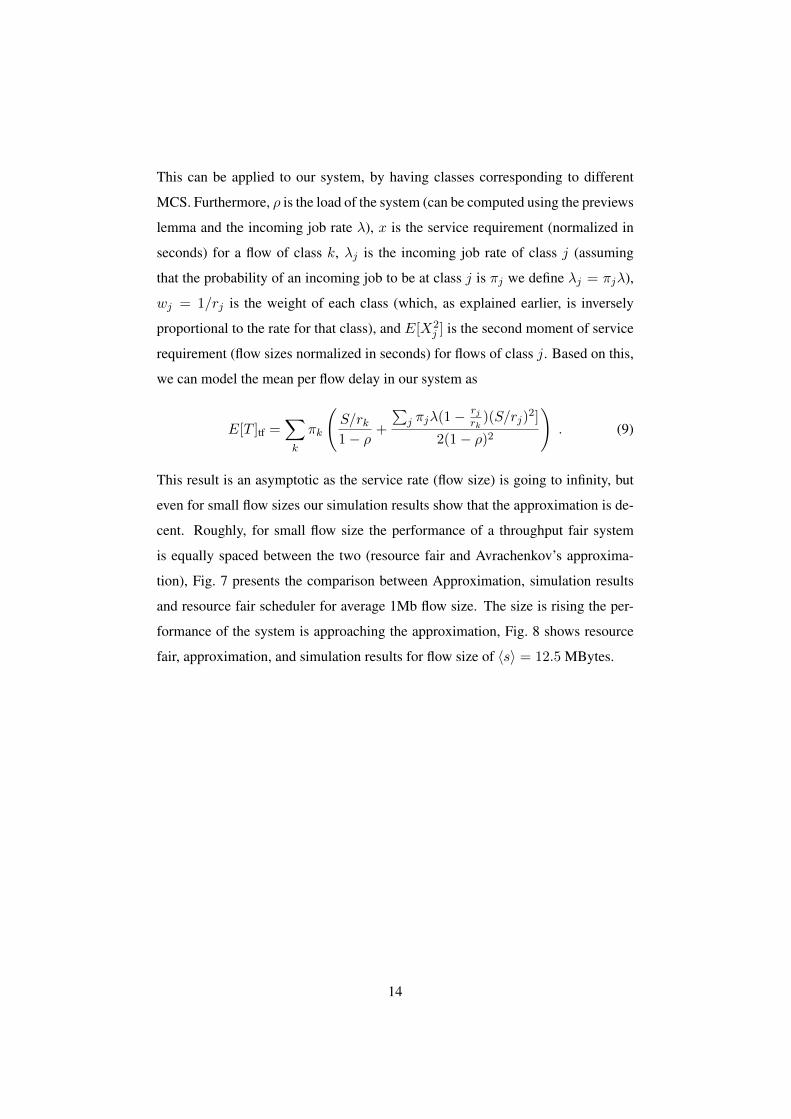
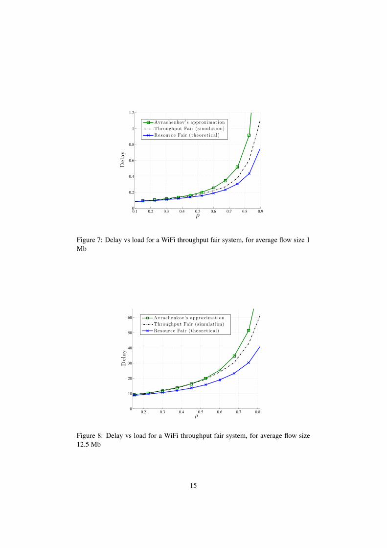
This result is an asymptotic as the service rate (flow size) is going to infinity, but
even for small flow sizes our simulation results show that the approximation is de-
cent. Roughly, for small flow size the performance of a throughput fair system
is equally spaced between the two (resource fair and Avrachenkov’s approxima-
tion), Fig. 7 presents the comparison between Approximation, simulation results
and resource fair scheduler for average 1Mb flow size. The size is rising the per-
formance of the system is approaching the approximation, Fig. 8 shows resource
fair, approximation, and simulation results for flow size of 〈s〉 = 12.5 MBytes.
14
0.1 0.2 0.3 0.4 0.5 0.6 0.7 0.8 0.90
0.2
0.4
0.6
0.8
1
1.2
ρ
Delay
Avrachenkov’s approximation
Throughput Fair (s imulat ion)
Resource Fair (theoret ical)
Figure 7: Delay vs load for a WiFi throughput fair system, for average flow size 1Mb
0.2 0.3 0.4 0.5 0.6 0.7 0.80
10
20
30
40
50
60
ρ
Delay
Avrachenkov’s approximation
Throughput Fair (s imulat ion)
Resource Fair (theoret ical)
Figure 8: Delay vs load for a WiFi throughput fair system, for average flow size12.5 Mb
15
References
[1] LTE Specifications, http://www.3gpp.org/DynaReport/36-series.htm.
[2] 802.11 Specifications, http://standards.ieee.org/about/get/802/802.11.html.
[3] “White paper: Ieee 802.11ac migration guide,” tech. rep., FLUKE networks,2015.
[4] OpenAir Interface, www.openairinterface.org.
[5] S. Sesia, I. Toufik, and M. Baker, LTE - the UMTS long term evolution : fromtheory to practice. Wiley, 2009.
[6] AirMagnet and inc, “802.11n Primer,” Whitepaper, 2008.
[7] G. Bianchi, “Performance analysis of the ieee 802.11 distributed coordinationfunction,” Selected Areas in Communications, IEEE Journal on, 2000.
[8] Y. Lin and V. Wong, “Wsn01-1: Frame aggregation and optimal frame sizeadaptation for ieee 802.11n wlans,” in GLOBECOM IEEE, 2006.
[9] S. Borst, “User-level performance of channel-aware scheduling algorithms inwireless data networks,” Networking, IEEE/ACM Transactions on Network-ing, 2005.
[10] T. Bonald and A. Proutiere, “Wireless downlink data channels: User perfor-mance and cell dimensioning,” in ACM MOBICOM, 2003.
[11] F. Capozzi, G. Piro, L. Grieco, G. Boggia, and P. Camarda, “Downlink packetscheduling in lte cellular networks: Key design issues and a survey,” Commu-nications Surveys Tutorials, IEEE, 2013.
[12] G. Fayolle, I. Mitrani, and R. Iasnogorodski, “Sharing a processor amongmany job classes,” J. ACM, 1980.
[13] S. Aalto, U. Ayesta, S. Borst, V. Misra, and R. Nunez Queija, “Beyond pro-cessor sharing,” in ACM SIGMETRICS, 2007.
[14] T. Bonald and J. Roberts, “Scheduling network traffic,” in ACM SIGMET-RICS, 2007.
[15] M. Heusse, F. Rousseau, G. Berger-Sabbatel, and A. Duda, “Performanceanomaly of 802.11b,” in INFOCOM IEEE, 2003.
[16] A. Karr, Probability. Springer, 1993.
[17] K. Avtachenkov, U. Ayesta, P. Brown, and R. Nunez Queija, “Discriminatoryprocessor sharing revisited,” INFOCOM, 2005.
16

![LTE PHY Layer Measurement Guide...4 LTE PHY Layer Measurement Guide LTE Downlink The LTE downlink can be set on six different frequency profiles, as follows: Channel Bandwidth [MHz]](https://img.pdfslide.us/doc/110x75/5e9903898496907a812cd628/lte-phy-layer-measurement-guide-4-lte-phy-layer-measurement-guide-lte-downlink.jpg)