Embed Size (px)
DESCRIPTION
Photovoltaic
Citation preview

PhotovoltaicSystems
EngineeringSECOND EDITION

CRC PR ESSBoca Raton London New York Washington, D.C.
PhotovoltaicSystems
EngineeringSECOND EDITION
Roger A. MessengerJerry Ventre

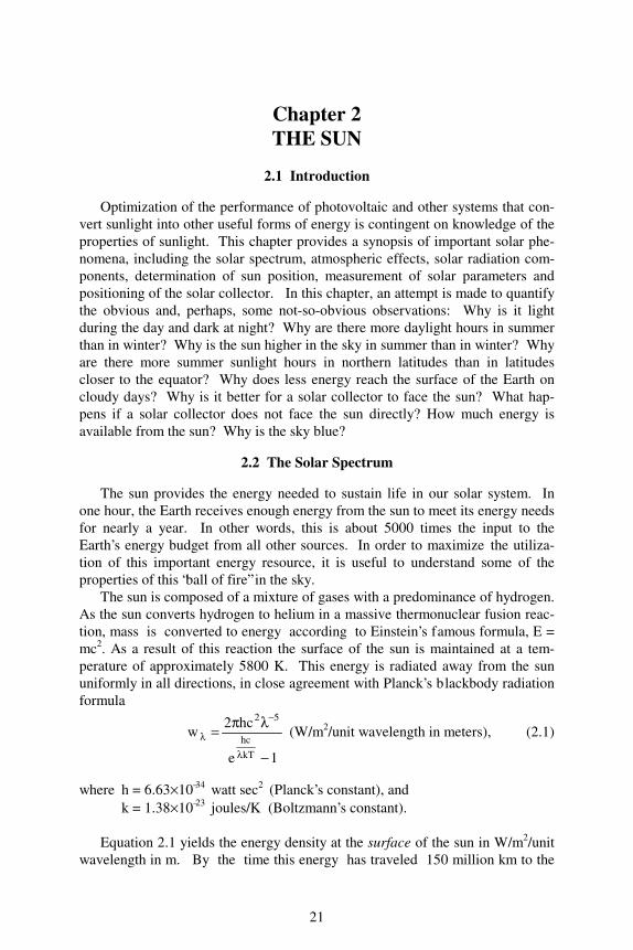
Photo Illustration: Steven C. Spencer, Florida Solar Energy Center
View of the Earth From Space, Western Hemisphere
: NASA Goddard Space Flight Center Image by RetoStöckli. Enhancements by Robert Simmon. Data and technical support: MODIS Land Group; MODISScience Data Support Team; MODIS Atmosphere Group; MODIS Ocean Group, USGS EROS DataCenter, USGS Terrestrial Remote Sensing Flagstaff Field Center..
This book contains information obtained from authentic and highly regarded sources. Reprinted materialis quoted with permission, and sources are indicated. A wide variety of references are listed. Reasonableefforts have been made to publish reliable data and information, but the author and the publisher cannotassume responsibility for the validity of all materials or for the consequences of their use.
Neither this book nor any part may be reproduced or transmitted in any form or by any means, electronicor mechanical, including photocopying, microÞlming, and recording, or by any information storage orretrieval system, without prior permission in writing from the publisher.
The consent of CRC Press LLC does not extend to copying for general distribution, for promotion, forcreating new works, or for resale. SpeciÞc permission must be obtained in writing from CRC Press LLCfor such copying.
Direct all inquiries to CRC Press LLC, 2000 N.W. Corporate Blvd., Boca Raton, Florida 33431.
Trademark Notice:
Product or corporate names may be trademarks or registered trademarks, and areused only for identiÞcation and explanation, without intent to infringe.
Visit the CRC Press Web site at www.crcpress.com
© 2004 by CRC Press LLC
No claim to original U.S. Government worksInternational Standard Book Number 0-8493-1793-2
Library of Congress Card Number 2003053063
Library of Congress Cataloging-in-Publication Data
Messenger, Roger.Photovoltaic systems engineering / Roger Messenger, Jerry Ventre.
2nd ed.p. cm.
Includes bibliographical references and index.ISBN 0-8493-1793-2 (alk. paper)
1. Photovoltaic power systems. 2. DwellingsPower supply. 3. Building-integrated photovoltaic systems. I. Ventre, Jerry. II. Title.
TK1087 .M47 2003621.31
¢
244dc21 2003053063
1793 disclaimer Page 1 Tuesday, June 17, 2003 11:28 AM
This edition published in the Taylor & Francis e-Library, 2005.
“To purchase your own copy of this or any of Taylor & Francis or Routledge’scollection of thousands of eBooks please go to www.eBookstore.tandf.co.uk.”
ISBN 0-203-50629-4 Master e-book ISBN
ISBN 0-203-58847-9 (Adobe eReader Format)
We did not inherit this world from our parents. . . .We are borrowing it from our children.
(Author unknown)
It is our fervent hope that the engineers who read this bookwill dedicate themselves to the creation of a world
where children and grandchildren will be leftwith air they can breathe and water they can drink,
where humans and the rest of naturewill nurture one another.

PREFACE
The goal of the first edition of this textbook was to present a comprehensiveengineering basis for photovoltaic (PV) system design, so the engineer wouldunderstand the what, the why and the how associated with electrical, mechanical,economic and aesthetic aspects of PV system design. The first edition was in-tended to educate the engineer in the design of PV systems so that when engi-neering judgment was needed, the engineer would be able to make intelligentdecisions based upon a clear understanding of the parameters involved. Thisgoal differentiated this textbook from the many design and installation manualsthat are currently available that train the reader how to do it, but not why.
Widespread acceptance of the first edition, coupled with significant growthand new ideas in the PV industry over the 3 years since its publication, alongwith 3 additional years of experience with PV system design and installation forthe authors, has led to the publication of this second edition. This edition in-cludes updates in all chapters, including a number of new homework problemsand sections that cover contemporary system designs in significant detail. Thebook is heavily design-oriented, with system examples based upon presentlyavailable system components (2003).
While the primary purpose of this material is for classroom use, with an em-phasis on the electrical components of PV systems, we have endeavored to pres-ent the material in a manner sufficiently comprehensive that it will also serve thepracticing engineer as a useful reference book.
The what question is addressed in the first three chapters, which present anupdated background of energy production and consumption, some mathematicalbackground for understanding energy supply and demand, a summary of the so-lar spectrum, how to locate the sun and how to optimize the capture of its en-ergy, as well as the various components that are used in PV systems. A sectionon shading has been added to Chapter 2, and Chapter 3 has been updated to in-clude multilevel H-bridge inverters and linear current boosters.
The why and how questions are dealt with in the remaining chapters in whichevery effort is made to explain why certain PV designs are done in certain ways,as well as how the design process is implemented. Included in the why part ofthe PV design criteria are economic and environmental issues that are discussedin Chapters 5 and 9. Chapter 6 has been embellished with additional practicalconsiderations added to the theoretical background associated with mechanicaldesign. Chapters 7 and 8 have been nearly completely reworked to incorporatethe most recently available technology and design and installation practice.
Appendix A has been extended to include horizontal and vertical array ori-entations along with the three array orientations covered in the first edition.Web sites have been updated in Appendix B, and a new Appendix C has beenadded that presents a recommended format for submittal of a PV design packagefor permitting or for design review.

A modified top-down approach is used in the presentation of the material.The material is organized to present a relatively quick exposure to all of thebuilding blocks of the PV system, followed by design, design and design. Eventhe physics of PV cells of Chapter 10 and the material on present and future cellsof Chapter 11 are presented with a design flavor. The focus is on adjusting theparameters of PV cells to optimize their performance, as well as on presentingthe physical basis of PV cell operation.
Homework problems are incorporated that require both analysis and design,since the ability to perform analysis is the precursor to being able to understandhow to implement good design. Many of the problems have multiple answers,such as “Calculate the number of daylight hours on the day you were bor n in thecity of your birth.” We have eliminated a few homework problem s based on oldtechnology and added a number of new problems based upon contemporarytechnology. Hopefully there is a sufficient number to enable students to testtheir understanding of the material.
We recommend that the course be presented so that by the end of Chapter 4,students will be able to think seriously about a comprehensive design project,and by the end of Chapter 7, they will be able to begin their design. We like toassign two design projects—a stand-alone system based on Chapte r 7 materialand a utility interactive system based on Chapter 8 material.
While it is possible to cover all the material in this textbook in a 3-creditsemester course, it may be necessary to skim over some of the topics. This iswhere the discretion of the instructor enters the picture. For example, each ofthe design examples of Chapter 4 introduces something new, but a few examplesmight be left as exercises for the reader with a preface by the instructor as towhat is new in the example. Alternatively, by summarizing the old material ineach example and then focusing on the new material, the why of the new con-cepts can be emphasized.
The order of presentation of the material actually seems to foster a genuinereader interest in the relevance and importance of the material. Subject mattercovers a wide range of topics, from chemistry to circuit analysis to electronics,solid state device theory and economics. The material is presented at a level thatcan best be understood by those who have reached upper division at the engi-neering undergraduate level and have also completed coursework in circuits andin electronics.
We recognize that the movement to reduce credit toward the bachelor’s de-gree has left many programs with less flexibility in the selection of undergradu-ate elective courses, and note that the material in this textbook can also be usedfor a beginning graduate level course.
One of the authors has twice taught the course as an internet course using thefirst edition of the book. Those students who were actually sufficiently moti-vated to keep up with the course generally reported that they found the text to bevery readable and a reasonable replacement for lectures. We highly recommendthat if the internet is tried, that quizzes be given frequently to coerce the student

into feeling that this course is just as important as her/his linear systems analysiscourse. Informal discussion sessions can also be useful in this regard.
The photovoltaic field is evolving rapidly. While every effort has been madeto present contemporary material in this work, the fact that it has evolved over aperiod of a year almost guarantees that by the time it is adopted, some of thematerial will be outdated. For the engineer who wishes to remain current in thefield, many of the references and web sites listed will keep him/her up-to-date.Proceedings of the many PV conferences, symposia and workshops, along withmanufacturers’ data, are especially helpful.
This textbook should provide the engineer with the intellectual tools neededfor understanding new technologies and new ideas in this rapidly emerging field.The authors hope that at least one in every 4.6837 students will make his/herown contribution to the PV knowledge pool.
We apologize at the outset for the occasional presentation of information thatmay be considered to be practical or, perhaps, even interesting or useful. Wefully recognize that engineering students expect the material in engineeringcourses to be of a highly theoretical nature with little apparent practical applica-tion. We have made every effort to incorporate heavy theory to satisfy this ap-petite whenever possible.


ACKNOWLEDGMENTS
We are convinced that it is virtually impossible to undertake and complete aproject such as this without the encouragement, guidance and assistance from ahost of friends, family and colleagues.
In particular, Jim Dunlop provided a diverse collection of ideas for us to de-velop and Neelkanth Dhere provided insight into the material in Chapters 10 and11. Paul Maycock was kind enough to share his latest data on worldwide PVshipments and installations. Iraida Rickling once again gave us invaluable li-brary reference support and Dianne Wood did an excellent job on the newChapter 6 illustrations. And, of course, student feedback on the first edition pro-vided significant insight to the authors on how to make the material easier tounderstand. We hope we have accomplished this goal.
We asked many questions of many people as we rounded up information forthe wide range of topics contained herein. A wealth of information flowed ourway from the National Renewable Energy Laboratory (NREL) and Sandia Na-tional Laboratories (SNL) as well as from many manufacturers and distributorsof a diverse range of PV system components. Special thanks to Dave Collier,Don Mayberry, Jr., John Wiles, Dale Tarrant, Martin Green, Ken Zweibel, TomKirk and Brad Bunn for the information they provided.
And, once again, Nancy Ventre was willing to forego the pleasure of Jerry’scompany while he engaged in his rewrite. We thank her for her support and un-derstanding.
Roger MessengerJerry Ventre2003

ABOUT THE AUTHORS
Roger Messenger is professor of Electrical Engineering at Florida AtlanticUniversity in Boca Raton, Florida. He received his Ph.D. in Electrical Engi-neering from the University of Minnesota and is a Registered Professional Engi-neer and a Certified Electrical Contractor, who enjoys working on a field instal-lation as much as he enjoys teaching a class or working on the design of a systemor contemplating the theory of operation of a system. His research work hasranged from electrical noise in gas discharge tubes to deep impurities in siliconto energy conservation. He worked on the development and promulgation of theoriginal Code for Energy Efficiency in Building Construction in Florida and hasconducted extensive field studies of energy consumption and conservation inbuildings and swimming pools.
During his tenure at Florida Atlantic University he has worked his waythrough the academic ranks and has also served in administrative posts for 11years, including Department Chair, Associate Dean and Director of the FAUCenter for Energy Conservation. He has received three university-wide awardsfor teaching over his 34 years at FAU, and currently advises half the under-graduate EE majors. Recently he has been actively involved with the FloridaSolar Energy Center in the development of courses, exams and study guides forvoluntary certification of PV installers.
Jerry Ventre is director of the Photovoltaics and Distributed Generation Di-vision of the Florida Solar Energy Center (FSEC), a research institute of theUniversity of Central Florida. He received his B.S., M.S., and Ph.D. degrees inaerospace engineering from the University of Cincinnati and has more than 30years of experience in various aspects of engineering, including research, devel-opment, design and systems analysis. He served on the aerospace engineeringfaculties of both the University of Cincinnati and the University of Central Flor-ida, is a Registered Professional Engineer, and, among many courses, taughtphotovoltaic systems at the graduate level. He has designed solid rocket motorsand jet engines for the Advanced Engine Technology Department of the GeneralElectric Company, and has performed research for numerous agencies, includingNASA, Sandia National Laboratories, Oak Ridge National Laboratory, U.S.Navy, the FAA and the U.S. Department of Energy. He has been active in tech-nical societies and has been the recipient of a number of awards for contributionsto engineering and engineering education.

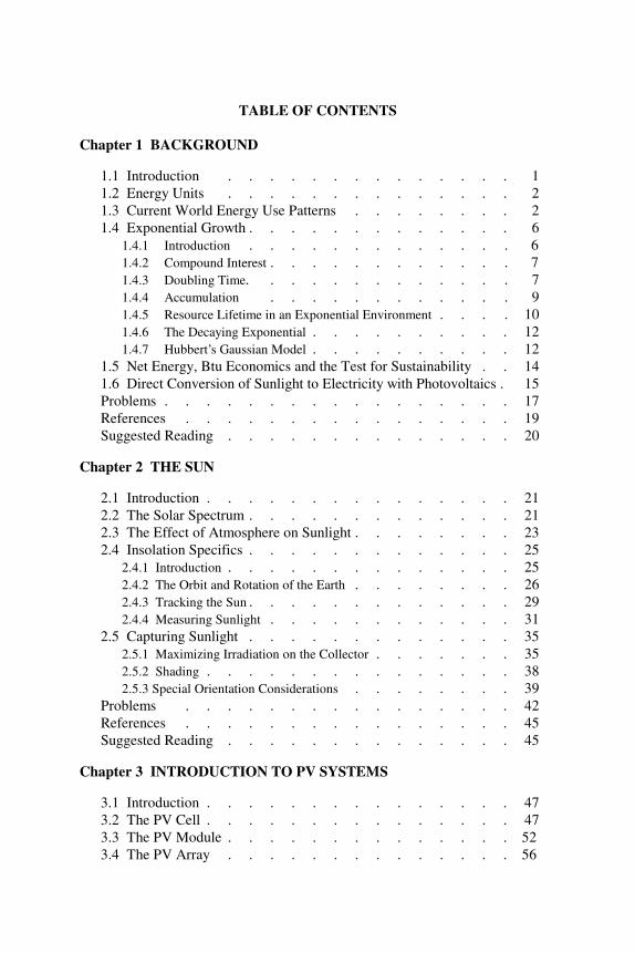
TABLE OF CONTENTS
Chapter 1 BACKGROUND
1.1 Introduction . . . . . . . . . . . . . . 11.2 Energy Units . . . . . . . . . . . . . . 21.3 Current World Energy Use Patterns . . . . . . . . 21.4 Exponential Growth . . . . . . . . . . . . . 6
1.4.1 Introduction . . . . . . . . . . . . . 61.4.2 Compound Interest . . . . . . . . . . . . 71.4.3 Doubling Time. . . . . . . . . . . . . 71.4.4 Accumulation . . . . . . . . . . . . 91.4.5 Resource Lifetime in an Exponential Environment . . . . 101.4.6 The Decaying Exponential . . . . . . . . . . 121.4.7 Hubbert’s Gaussian Model . . . . . . . . . . 12
1.5 Net Energy, Btu Economics and the Test for Sustainability . . 141.6 Direct Conversion of Sunlight to Electricity with Photovoltaics . 15Problems . . . . . . . . . . . . . . . . . 17References . . . . . . . . . . . . . . . . 19Suggested Reading . . . . . . . . . . . . . . 20
Chapter 2 THE SUN
2.1 Introduction . . . . . . . . . . . . . . . 212.2 The Solar Spectrum . . . . . . . . . . . . . 212.3 The Effect of Atmosphere on Sunlight . . . . . . . . 232.4 Insolation Specifics . . . . . . . . . . . . . 25
2.4.1 Introduction . . . . . . . . . . . . . . 252.4.2 The Orbit and Rotation of the Earth . . . . . . . . 262.4.3 Tracking the Sun . . . . . . . . . . . . . 292.4.4 Measuring Sunlight . . . . . . . . . . . . 31
2.5 Capturing Sunlight . . . . . . . . . . . . . 352.5.1 Maximizing Irradiation on the Collector . . . . . . . 352.5.2 Shading . . . . . . . . . . . . . . . 382.5.3 Special Orientation Considerations . . . . . . . . 39
Problems . . . . . . . . . . . . . . . . 42References . . . . . . . . . . . . . . . . 45Suggested Reading . . . . . . . . . . . . . . 45
Chapter 3 INTRODUCTION TO PV SYSTEMS
3.1 Introduction . . . . . . . . . . . . . . . 473.2 The PV Cell . . . . . . . . . . . . . . . 473.3 The PV Module . . . . . . . . . . . . . . 523.4 The PV Array . . . . . . . . . . . . . . 56
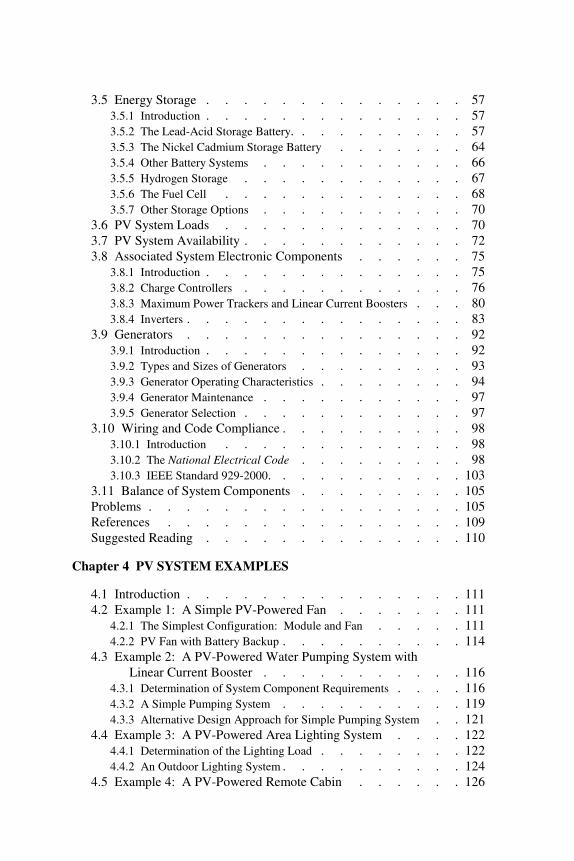
3.5 Energy Storage . . . . . . . . . . . . . . 573.5.1 Introduction . . . . . . . . . . . . . . 573.5.2 The Lead-Acid Storage Battery. . . . . . . . . . 573.5.3 The Nickel Cadmium Storage Battery . . . . . . . 643.5.4 Other Battery Systems . . . . . . . . . . . 663.5.5 Hydrogen Storage . . . . . . . . . . . . 673.5.6 The Fuel Cell . . . . . . . . . . . . . 683.5.7 Other Storage Options . . . . . . . . . . . 70
3.6 PV System Loads . . . . . . . . . . . . . 703.7 PV System Availability . . . . . . . . . . . . 723.8 Associated System Electronic Components . . . . . . 75
3.8.1 Introduction . . . . . . . . . . . . . . 753.8.2 Charge Controllers . . . . . . . . . . . . 763.8.3 Maximum Power Trackers and Linear Current Boosters . . . 803.8.4 Inverters . . . . . . . . . . . . . . . 83
3.9 Generators . . . . . . . . . . . . . . . 923.9.1 Introduction . . . . . . . . . . . . . . 923.9.2 Types and Sizes of Generators . . . . . . . . . 933.9.3 Generator Operating Characteristics . . . . . . . . 943.9.4 Generator Maintenance . . . . . . . . . . . 973.9.5 Generator Selection . . . . . . . . . . . . 97
3.10 Wiring and Code Compliance . . . . . . . . . . 983.10.1 Introduction . . . . . . . . . . . . . 983.10.2 The National Electrical Code . . . . . . . . . 983.10.3 IEEE Standard 929-2000. . . . . . . . . . . 103
3.11 Balance of System Components . . . . . . . . . 105Problems . . . . . . . . . . . . . . . . . 105References . . . . . . . . . . . . . . . . 109Suggested Reading . . . . . . . . . . . . . . 110
Chapter 4 PV SYSTEM EXAMPLES
4.1 Introduction . . . . . . . . . . . . . . . 1114.2 Example 1: A Simple PV-Powered Fan . . . . . . . 111
4.2.1 The Simplest Configuration: Module and Fan . . . . . 1114.2.2 PV Fan with Battery Backup . . . . . . . . . . 114
4.3 Example 2: A PV-Powered Water Pumping System withLinear Current Booster . . . . . . . . . . . 116
4.3.1 Determination of System Component Requirements . . . . 1164.3.2 A Simple Pumping System . . . . . . . . . . 1194.3.3 Alternative Design Approach for Simple Pumping System . . 121
4.4 Example 3: A PV-Powered Area Lighting System . . . . 1224.4.1 Determination of the Lighting Load . . . . . . . . 1224.4.2 An Outdoor Lighting System . . . . . . . . . . 124
4.5 Example 4: A PV-Powered Remote Cabin . . . . . . 126

4.6 Example 5: A Hybrid System . . . . . . . . . . 1284.7 Example 6: A Utility Interactive System . . . . . . . 130
4.7.1 Introduction . . . . . . . . . . . . . . 1304.7.2 A Simple Utility Interactive System with No Battery Storage . . 132
4.8 Example 7: A Cathodic Protection System . . . . . . 1344.8.1 Introduction . . . . . . . . . . . . . . 1344.8.2 System Design . . . . . . . . . . . . . 135
4.9 Example 8: A Portable Highway Advisory Sign . . . . . 1384.9.1 Introduction . . . . . . . . . . . . . . 1384.9.2 Determination of Available Average Power . . . . . . 139
Problems . . . . . . . . . . . . . . . . . 141References . . . . . . . . . . . . . . . . 143Suggested Reading . . . . . . . . . . . . . . 143
Chapter 5 COST CONSIDERATIONS
5.1 Introduction . . . . . . . . . . . . . . . 1455.2 Life Cycle Costing . . . . . . . . . . . . . 145
5.2.1 The Time Value of Money . . . . . . . . . . 1455.2.2 Present Worth Factors and Present Worth . . . . . . 1485.2.3 Life Cycle Cost . . . . . . . . . . . . . 1495.2.4 Annualized Life Cycle Cost . . . . . . . . . . 1515.2.5 Unit Electrical Cost . . . . . . . . . . . . 152
5.3 Borrowing Money . . . . . . . . . . . . . 1525.3.1 Introduction . . . . . . . . . . . . . . 1525.3.2 Determination of Annual Payments on Borrowed Money . . . 1525.3.3 The Effect of Borrowing on Life Cycle Cost . . . . . . 154
5.4 Externalities . . . . . . . . . . . . . . . 1555.4.1 Introduction . . . . . . . . . . . . . . 1555.4.2 Subsidies . . . . . . . . . . . . . . 1565.4.3 Externalities and Photovoltaics . . . . . . . . . 157
Problems . . . . . . . . . . . . . . . . . 157References . . . . . . . . . . . . . . . . 158Suggested Reading . . . . . . . . . . . . . . 158
Chapter 6 MECHANICAL CONSIDERATIONS
6.1 Introduction . . . . . . . . . . . . . . . 1596.2 Important Properties of Materials . . . . . . . . . 159
6.2.1 Introduction . . . . . . . . . . . . . . 1596.2.2 Mechanical Properties . . . . . . . . . . . 1616.2.3 Stress and Strain . . . . . . . . . . . . . 1636.2.4 Strength of Materials. . . . . . . . . . . . 1666.2.5 Column Buckling . . . . . . . . . . . . 1676.2.6 Thermal Expansion and Contraction . . . . . . . . 167
6.2.7 Chemical Corrosion and Ultraviolet Degradation . . . . . 1696.2.8 Properties of Steel . . . . . . . . . . . . 1726.2.9 Properties of Aluminum . . . . . . . . . . . 173
6.3 Establishing Mechanical System Requirements . . . . . 1746.3.1 Mechanical System Design Process . . . . . . . . 1746.3.2 Functional Requirements . . . . . . . . . . . 1756.3.3 Operational Requirements . . . . . . . . . . 1766.3.4 Constraints . . . . . . . . . . . . . . 1766.3.5 Tradeoffs . . . . . . . . . . . . . . 177
6.4 Design and Installation Guidelines . . . . . . . . . 1776.4.1 Standards and Codes . . . . . . . . . . . . 1776.4.2 Building Code Requirements . . . . . . . . . . 179
6.5 Forces Acting on Photovoltaic Arrays . . . . . . . . 1796.5.1 Structural Loading Considerations . . . . . . . . 1796.5.2 Dead Loads . . . . . . . . . . . . . . 1806.5.3 Live Loads . . . . . . . . . . . . . . 1816.5.4 Wind Loads . . . . . . . . . . . . . . 1816.5.5 Snow Loads . . . . . . . . . . . . . . 1896.5.6 Other Loads . . . . . . . . . . . . . . 189
6.6 Array Mounting System Design . . . . . . . . . 1906.6.1 Introduction . . . . . . . . . . . . . . 1906.6.2 Objectives in Designing the Array Mounting System . . . . 1906.6.3 Enhancing Array Performance . . . . . . . . . 1936.6.4 Roof-Mounted Arrays . . . . . . . . . . . 1946.6.5 Ground-Mounted Arrays . . . . . . . . . . . 1976.6.6 Aesthetics . . . . . . . . . . . . . . 199
6.7 Computing Mechanical Loads and Stresses . . . . . . 2006.7.1 Introduction . . . . . . . . . . . . . . 2006.7.2 Withdrawal Loads . . . . . . . . . . . . 2006.7.3 Tensile Stresses . . . . . . . . . . . . . 2016.7.4 Buckling . . . . . . . . . . . . . . . 202
6.8 Summary . . . . . . . . . . . . . . . 203Problems . . . . . . . . . . . . . . . . . 204References . . . . . . . . . . . . . . . . 207Suggested Reading . . . . . . . . . . . . . . 208
Chapter 7 STAND-ALONE PV SYSTEMS
7.1 Introduction . . . . . . . . . . . . . . . 2097.2 A Critical Need Refrigeration System . . . . . . . . 210
7.2.1 Design Specifications . . . . . . . . . . . 2107.2.2 Design Implementation . . . . . . . . . . . 210
7.3 A PV-Powered Mountain Cabin . . . . . . . . . 2247.3.1 Design Specifications . . . . . . . . . . . 2247.3.2 Design Implementation . . . . . . . . . . . 225
7.4 A Hybrid Powered Residence . . . . . . . . . . 2357.4.1 Design Specifications . . . . . . . . . . . 2357.4.2 Design Implementation . . . . . . . . . . . 236
7.5 Seasonal or Periodic Battery Discharge . . . . . . . 2487.6 Battery Connections . . . . . . . . . . . . 2497.7 Computer Programs . . . . . . . . . . . . . 253Problems . . . . . . . . . . . . . . . . . 254References . . . . . . . . . . . . . . . . 257Suggested Reading . . . . . . . . . . . . . . 257
Chapter 8 UTILITY INTERACTIVE PV SYSTEMS
8.1 Introduction . . . . . . . . . . . . . . . 2598.2 Nontechnical Barriers to Utility Interactive PV Systems . . . 260
8.2.1 Cost of PV Arrays . . . . . . . . . . . . 2608.2.2 Cost of Balance of System Components . . . . . . . 2618.2.3 Standardization of Interconnection Requirements . . . . . 2628.2.4 PV System Installation Considerations . . . . . . . 2628.2.5 Metering of PV System Output . . . . . . . . . 263
8.3 Technical Considerations for Connecting to the Grid. . . . . 2648.3.1 Introduction . . . . . . . . . . . . . . 2648.3.2 IEEE Standard 929-2000 Issues . . . . . . . . . 2658.3.3 National Electrical Code Considerations. . . . . . . 2718.3.4 Other Issues . . . . . . . . . . . . . . 279
8.4 Small (<10 kW) Utility Interactive PV Systems . . . . . 2818.4.1 Introduction . . . . . . . . . . . . . . 2818.4.2 Array Installation . . . . . . . . . . . . 2838.4.3 PCU Selection and Mounting . . . . . . . . . 2838.4.4 Other Installation Considerations . . . . . . . . . 2848.4.5 A 2.5 kW Residential Rooftop Utility Interactive PV System . . 2858.4.6 A Residential Rooftop System Using AC Modules . . . . 2898.4.7 A 4800 W Residential Rooftop System with Battery Storage . . 290
8.5 Medium Utility Interactive PV Systems . . . . . . . 2998.5.1 Introduction . . . . . . . . . . . . . . 2998.5.2 A 16 kW Commercial Rooftop System . . . . . . . 299
8.6 Large Utility Interactive PV Systems . . . . . . . . 3038.6.1 Introduction . . . . . . . . . . . . . . 3038.6.2 A Large Parking Lot PV System . . . . . . . . . 303
Problems . . . . . . . . . . . . . . . . . 312References . . . . . . . . . . . . . . . . 316Suggested Reading . . . . . . . . . . . . . . 317
Chapter 9 EXTERNALITIES AND PHOTOVOLTAICS
9.1 Introduction . . . . . . . . . . . . . . . 3199.2 Externalities . . . . . . . . . . . . . . . 3199.3 Environmental Effects of Energy Sources . . . . . . 321
9.3.1 Introduction . . . . . . . . . . . . . . 3219.3.2 Air Pollution. . . . . . . . . . . . . . 3229.3.3 Water and Soil Pollution . . . . . . . . . . . 3239.3.4 Infrastructure Degradation . . . . . . . . . . 3249.3.5 Quantifying the Cost of Externalities. . . . . . . . 3249.3.6 Health and Safety as Externalities . . . . . . . . 328
9.4 Externalities Associated with PV Systems. . . . . . . 3289.4.1 Environmental Effects of PV System Production . . . . . 3289.4.2 Environmental Effects of PV System Deployment
and Operation . . . . . . . . . . . . . . 3309.4.3 Environmental Effects of PV System Decommissioning . . . 331
Problems . . . . . . . . . . . . . . . . . 332References . . . . . . . . . . . . . . . . 332
Chapter 10 THE PHYSICS OF PHOTOVOLTAIC CELLS
10.1 Introduction . . . . . . . . . . . . . . 33510.2 Optical Absorption . . . . . . . . . . . . . 335
10.2.1 Introduction . . . . . . . . . . . . . 33510.2.2 Semiconductor Materials . . . . . . . . . . 33510.2.3 Generation of EHP by Photon Absorption . . . . . . 33710.2.4 Photoconductors . . . . . . . . . . . . 339
10.3 Extrinsic Semiconductors and the pn Junction . . . . . 34110.3.1 Extrinsic Semiconductors . . . . . . . . . . 34110.3.2 The pn Junction . . . . . . . . . . . . . 343
10.4 Maximizing PV Cell Performance . . . . . . . . 35210.4.1 Introduction . . . . . . . . . . . . . 35210.4.2 Minimizing the Reverse Saturation Current . . . . . . 35210.4.3 Optimizing Photocurrent . . . . . . . . . . 35310.4.4 Minimizing Cell Resistance Losses . . . . . . . . 362
10.5 Exotic Junctions . . . . . . . . . . . . . 36410.5.1 Introduction . . . . . . . . . . . . . 36410.5.2 Graded Junctions . . . . . . . . . . . . 36410.5.3 Heterojunctions . . . . . . . . . . . . . 36610.5.4 Schottky Junctions . . . . . . . . . . . . 36610.5.5 Multijunctions . . . . . . . . . . . . . 36910.5.6 Tunnel Junctions . . . . . . . . . . . . 369
Problems . . . . . . . . . . . . . . . . . 371References . . . . . . . . . . . . . . . . 372

Chapter 11 PRESENT AND PROPOSED PV CELLS
11.1 Introduction . . . . . . . . . . . . . . 37311.2 Silicon PV Cells . . . . . . . . . . . . . 374
11.2.1 Production of Pure Silicon . . . . . . . . . . 37511.2.2 Single Crystal Silicon Cells . . . . . . . . . . 37611.2.3 Multicrystalline Silicon Cells . . . . . . . . . 38311.2.4 Buried Contact Silicon Cells . . . . . . . . . 38411.2.5 Other Thin Silicon Cells . . . . . . . . . . 38611.2.6 Amorphous Silicon Cells . . . . . . . . . . 386
11.3 Gallium Arsenide Cells . . . . . . . . . . . 38911.3.1 Introduction . . . . . . . . . . . . . 38911.3.2 Production of Pure Cell Components . . . . . . . 38911.3.3 Fabrication of the Gallium Arsenide Cell . . . . . . 39211.3.4 Cell Performance . . . . . . . . . . . . 394
11.4 Copper Indium (Gallium) Diselenide Cells . . . . . . 39411.4.1 Introduction . . . . . . . . . . . . . 39411.4.2 Production of Pure Cell Components . . . . . . . 39511.4.3 Fabrication of the CIS Cell . . . . . . . . . . 39811.4.4 Cell Performance . . . . . . . . . . . . 400
11.5 Cadmium Telluride Cells . . . . . . . . . . . 40111.5.1 Introduction . . . . . . . . . . . . . 40111.5.2 Production of Pure Tellurium . . . . . . . . . 40211.5.3 Production of the CdTe Cell . . . . . . . . . 40211.5.4 Cell Performance . . . . . . . . . . . . 404
11.6 Emerging Technologies . . . . . . . . . . . 40411.6.1 New Developments in Silicon Technology . . . . . . 40411.6.2 CIS-Family-Based Absorbers . . . . . . . . . 40611.6.3 Other III-V and II-VI Emerging Technologies . . . . . 40711.6.4 Other Technologies . . . . . . . . . . . . 40811.6.5 Summary . . . . . . . . . . . . . . 410
Problems . . . . . . . . . . . . . . . . . 410References . . . . . . . . . . . . . . . . 411Suggested Reading . . . . . . . . . . . . . . 413
Appendix A Average Daily Irradiation for Selected Cities . . . . 415Appendix B A Partial Listing of PV-Related Web Sites . . . . . 431Appendix C Design Review Checklist . . . . . . . . . 433Index . . . . . . . . . . . . . . . . . . . 437

1
Chapter 1BACKGROUND
The Million Solar Roofs Initiative
On June 26, 1997, U.S. President Bill Clinton announced the Million SolarRoofs Initiative (MSRI) to the United Nations Special Session on Environmentand Development in New York [1]. “Now we will work with businesses andcommunities to use the sun’s energy to reduce our reliance on fossil fuels byinstalling solar panels on 1 million more roofs around our nation by 2010. Cap-turing the sun’s warmth can help us to turn down the Earth’s te mperature.”
The following day, U.S. Secretary of Energy Federico Peña commented onthe projected accomplishments of the Million Solar Roofs Initiative [2]:
• Slow greenhouse gas emissions • Expand our energy options • Create high-technology jobs • Build on existing momentum • Keep U.S. companies competitive • Rely on market forces and consumer choice • Marshal existing federal resources
Implementation of this ambitious program requires engineers who are knowl-edgeable in photovoltaic system design. These engineers need to understand thewhy of photovoltaic systems in order to be able to make intelligent system de-sign choices. Success of the million solar roofs program should provide themomentum for a sustained effort in the deployment of solar technologies wellbeyond the year 2010. In fact, the MSRI may need to be extended to a 100 Mil-lion Solar Roofs Initiative to meet the sustainable energy needs of future genera-tions. This book is dedicated to the engineers and technicians who have beenand may become involved in turning this dream into reality.
1.1 Introduction
The human population of the earth has now passed 6 billion [3], and all ofthese inhabitants want the energy necessary to sustain their lives. Exactly howmuch energy is required to meet these needs and exactly what sources of energywill meet these needs will be questions to be addressed by the present and byfuture generations. One certainty, however, is that developing nations will beincreasing their per capita energy use significantly. For example, in 1997, thePeoples Republic of China was building electrical generating plants at the rate of300 megawatts per week. These plants have been using relatively inexpensive,old, inefficient, coal-fired technology and provide electricity to predominantlyinefficient end uses [4]. The potential consequences to the planet of continua-
Photovoltaic Systems Engineering2
tion of this effort are profound. Before we proceed with the details of photovol-taic power systems, a promising source of energy for the future, it is instructiveto look at the current technical and economic energy picture. This look will en-able the reader to better assess the contributions that engineers will need to maketoward a sustainable energy future for the planet.
1.2 Energy Units
Energy is measured in a number of ways, including the calorie, the Btu, thequad, the foot-pound and the kilowatt hour. For the benefit of those who maynot have memorized the appendices of their freshman physics books, we repeatthe definitions of these quantities for an earth-based system at or about a tem-perature of 27oC [5].
1 calorie is the heat needed to raise the temperature of 1 ml of water 1oC.1 Btu is the heat needed to raise the temperature of 1 lb of water 1oF.1 quad is 1 quadrillion (1015) Btus.1 foot-pound is the energy expended in raising 1 lb through a distance of 1 ft.1 kilowatt hour is the energy expended by 1 kilowatt operating for 1 hour.
With these definitions, the following equivalencies can be determined:
1 Btu = 252 calories1 kWh = 3413 Btu = 2,655,000 ft-lb1 ft-lb = 0.001285 Btu1 quad = 2.930 × 10¹¹ kWh
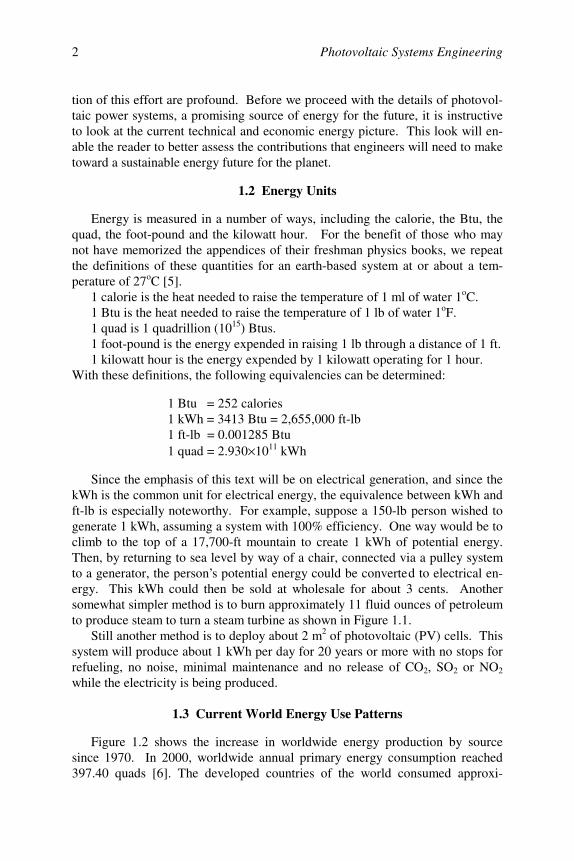
Since the emphasis of this text will be on electrical generation, and since thekWh is the common unit for electrical energy, the equivalence between kWh andft-lb is especially noteworthy. For example, suppose a 150-lb person wished togenerate 1 kWh, assuming a system with 100% efficiency. One way would be toclimb to the top of a 17,700-ft mountain to create 1 kWh of potential energy.Then, by returning to sea level by way of a chair, connected via a pulley systemto a generator, the person’s potential energy could be converted to electrical en-ergy. This kWh could then be sold at wholesale for about 3 cents. Anothersomewhat simpler method is to burn approximately 11 fluid ounces of petroleumto produce steam to turn a steam turbine as shown in Figure 1.1.
Still another method is to deploy about 2 m2 of photovoltaic (PV) cells. Thissystem will produce about 1 kWh per day for 20 years or more with no stops forrefueling, no noise, minimal maintenance and no release of CO2, SO2 or NO2
while the electricity is being produced.
1.3 Current World Energy Use Patterns
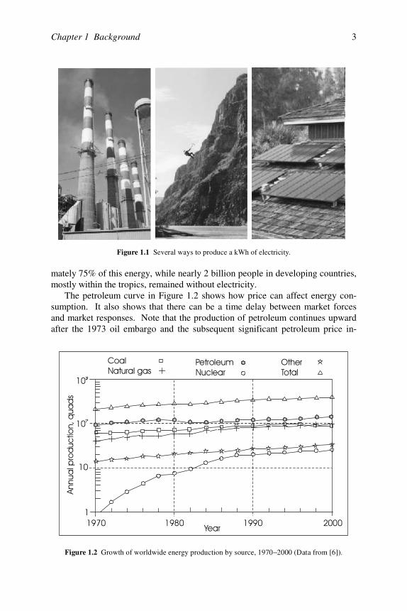
Figure 1.2 shows the increase in worldwide energy production by sourcesince 1970. In 2000, worldwide annual primary energy consumption reached397.40 quads [6]. The developed countries of the world consumed approxi-
Chapter 1 Background 3
mately 75% of this energy, while nearly 2 billion people in developing countries,mostly within the tropics, remained without electricity.
The petroleum curve in Figure 1.2 shows how price can affect energy con-sumption. It also shows that there can be a time delay between market forcesand market responses. Note that the production of petroleum continues upwardafter the 1973 oil embargo and the subsequent significant petroleum price in-
Figure 1.1 Several ways to produce a kWh of electricity.
Figure 1.2 Growth of worldwide energy production by source, 1970 2000 (Data from [6− ]).
Photovoltaic Systems Engineering4
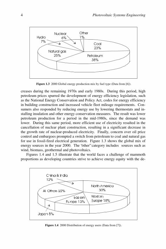
creases during the remaining 1970s and early 1980s. During this period, highpetroleum prices spurred the development of energy efficiency legislation, suchas the National Energy Conservation and Policy Act, codes for energy efficiencyin building construction and increased vehicle fleet mileage requirements. Con-sumers also responded by reducing energy use by lowering thermostats and in-stalling insulation and other energy conservation measures. The result was lowerpetroleum production for a period in the mid-1980s, since the demand waslower. During this same period, more efficient use of electricity resulted in thecancellation of nuclear plant construction, resulting in a significant decrease inthe growth rate of nuclear-produced electricity. Finally, concern over oil pricecontrol and embargoes prompted a switch from petroleum to coal and natural gasfor use in fossil-fired electrical generation. Figure 1.3 shows the global mix ofenergy sources in the year 2000. The “other” category includes sources such aswind, biomass, geothermal and photovoltaics.
Figures 1.4 and 1.5 illustrate that the world faces a challenge of mammothproportions as developing countries strive to achieve energy equity with the de-
!"
!"
#"
$%"
&"
"
Figure 1.3 2000 Global energy production mix by fuel type (Data from [6]).
1RUWK$PHULFD
:HVWHUQ
(XURSH(DVWHUQ
(XURSH
-DSDQ
$OO2WKHUV
&KLQD,QGLD
Figure 1.4 2000 Distribution of energy users (Data from [7]).
Chapter 1 Background 5
veloped countries. Note that energy equity is simply another term for the at-tempt to achieve comparable standards of living. But achieving a higher stan-dard of living can carry with it a price. The price includes not only monetaryobligations, but also the potential for significant environmental degradation ifenergy equity is pursued via the least expensive, first-cost options. Regrettably,this is the most probable scenario, since it is already underway in regions such asEastern Europe and Asia. In fact, it is probably more likely that use of least-costenergy options may lead to comparable per capita energy use, but may simulta-neously degrade the standard of living by producing air not suitable for breathingand water not suitable for drinking. These issues with be dealt with in more de-tail in Chapter 9.
Figure 1.4 shows that North America, with slightly more than 5% of theworld population, consumes 30% of the world’s energy, while China and India,with nearly one third of the world’s population, consume 12% of the world’senergy. What is missing in Figure 1.4 is the efficiency with which the energy isconsumed in these regions.
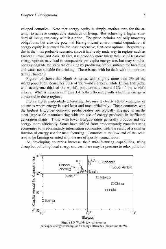
Figure 1.5 is particularly interesting, because it clearly shows examples ofcountries where energy is used least and most efficiently. Those countries withthe highest Btu/gross domestic product-ratios are typically engaged in ineffi-cient-large-scale manufacturing with the use of energy produced in inefficientgeneration plants. Those with lower Btu/gdp ratios generally produce and useenergy more efficiently. Some have shifted from predominantly manufacturingeconomies to predominantly information economies, with the result of a smallerfraction of energy use for manufacturing. Countries at the low end of the scaletend to be farming-oriented with the use of mostly manual labor.
As developing countries increase their manufacturing capabilities, usingcheap but polluting local energy sources, there may be pressure to relax pollution
'(
'
)*+**
+,
'
-
. /
01
- +
)*2*
Figure 1.5 Worldwide variations in per capita energy consumption vs energy efficiency (Data from [8, 9]).
Photovoltaic Systems Engineering6
control standards within the developed world in order to maintain the ability tocompete with production from developing countries. Opposition to free tradeagreements has been partially based on such environmental concerns, since suchagreements forbid any country to impose import tariffs on goods produced incountries having weak environmental standards. So the developed countries arechallenged to export efficiency to the developing countries.
But what does this discussion have to do with photovoltaic power produc-tion? Simple. As will be shown in Chapter 9, photovoltaic energy sources arevery clean, but current photovoltaic deployment costs cannot compete with theinitial installed costs of fossil sources of electrical generation in most cases. Itmeans that the consumer must be familiar with life-cycle costing and that theengineer must be able to create the most cost-effective photovoltaic solution. Italso means that a significant amount of research and development must be doneto ensure the continuation of the decrease in the price of photovoltaic generation.It also means that work must continue in the effort to put a price tag on environ-mental degradation caused by energy sources, so this price can be factored intothe total cost to society of any energy source.
The bottom line is that there remains a significant amount of work in re-search, development and public education to be done in the energy field, andparticularly in the field of photovoltaics. And much of this work can best bedone by knowledgeable engineers who, for example, understand the concept ofexponential growth.
1.4 Exponential Growth
1.4.1 Introduction
Exponential growth is probably most familiar to the electrical engineer in thediode equation, which relates diode current, I, to diode voltage, V
)1e(II kT
qV
o −= . (1.1)
While this equation is fundamental to the performance of photovoltaic cells,many other physical processes are also characterized by exponential growth.
Exponential growth is commonly referred to as compound interest. Almosteveryone has heard about it, but few understand the ramifications of constantannual percentage increase in a quantity, whether it be money, population, orenergy supply or demand. One of the first to warn of the dangers of exponentialgrowth was Malthus in 1798 [10]. He warned that population growth wouldexceed the ability to feed the population. The Malthusian theory is often thesubject of ridicule of growth enthusiasts [11]. The intent of this discussion isneither to support nor discount the predictions of Malthus, but merely to illus-trate an important mathematical principle that engineers often overlook. Theapplication of the principles of exponential growth is widespread in society, so
Chapter 1 Background 7
the principles of exponential growth should be just as important to a well-informed engineer as is the second law of thermodynamics. For those who mayhave missed the second law of thermodynamics in either chemistry or thermody-namics class, it is a statement that in every process less energy comes out thanwhat is put in. In other words, there is no free lunch.
1.4.2 Compound Interest
Compound interest is the process of compounding simple interest. If a quan-tity No is subject to an interest rate i, with i expressed as a fraction (i.e., i =%/100), the quantity will increase (or decrease, if i<0) to a value of
)i1(N)1(N o += (1.2)
after one prescribed time period has elapsed. If the quantity present after theprescribed time period is allowed to remain and to continue to accumulate at thesame rate, then the quantity is subject to compound interest and the amount pres-ent after n time periods will be
no )i1(N)n(N += . (1.3)
To show that this formula is a form of the exponential function, one needonly recall that
.ey ylnxx =
Hence,
.eN)n(N )i1ln(no
+= (1.4)
Some special properties of the exponential function can now be considered.
1.4.3 Doubling Time
To determine the time, D, it will take for the original quantity to double, oneneed only set N(n) = 2No and solve for n. The result (and the answer to problem1.1) is
n = D)i1ln(
2ln =+
. (1.5)
For small values of i, ln(1+i) can be approximated as ln(1+i) ≅ i. Noting thatln 2 = 0.693 leads to the formula so popular in the financial world, i.e.,
D = n ≅ 0.7/i. (1.6)
Hence, for an interest rate of 7% per year (i = 0.07), the doubling time willbe 10 years. For an interest rate of 10%, the doubling time will be approxi-
Photovoltaic Systems Engineering8
mately 7 years. However, as the interest rate exceeds 10%, the approximationbecomes less valid, and the exact expression should be used for accurate results.In the case where the interest rate is negative, it should be obvious that no dou-bling can occur. The authors have proven this to be the case with various in-vestments in the stock market.
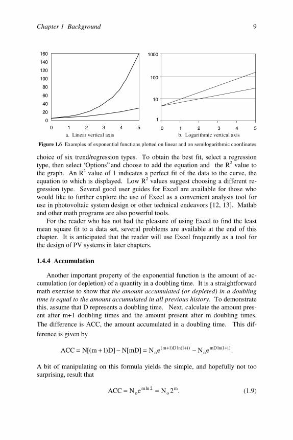
An important property of the exponential function is that the doubling proc-ess continues for all time. Hence, if the doubling time is 10 years, then thequantity will double again in another 10 years, so it will now be 4 times its origi-nal value. In another 10 years it will double again to 8 times its original value.After 40 years, the quantity will be 16 times its original value. Figure 1.6 showsthis exponential increase.
Note that if the function y = Aebx = A10bxloge is plotted with linear coordi-nates, the familiar exponential curve appears, as in Figure 1.6a. If the logarithmof each side is taken, the result is
x)elogb(Alogylog += . (1.7)
Hence, if log y is plotted as a function of x, the graph will be linear with slope blog e, as shown in Figure 1.6b. Figure 1.6b shows that plotting log y vs. x is aconvenient way to check for an exponential relationship between two variables.Notice also that the vertical axis can be labeled either in terms of log y or, sim-ply, in terms of y. When the axis is labeled in terms of y, it is understood thatthe axis is linear in the logarithm of y.
The values of A and b can be determined easily from the semilog plot. Theintercept of the function and the y-axis (x = 0) yields the value of A, providedthat the y-axis is labeled in terms of y. The slope can be calculated from asemilog plot by evaluating
=−−
=12
12
xx
ylogylogslope
)elogb(xx
]x)elogb(A[logx)elogb(Alog
12
12 =−
+−+. (1.8)
For the person who prefers to let computers do the work, either Excel orMatlab can conveniently plot data and produce a least mean square curve fit tothe data along with an estimate of the goodness of the fit. When a set of data isavailable, all one needs to do is to list the independent and dependent variablesside-by-side on an Excel spreadsheet and then use the Chart Wizard to plot an x-y scatter plot of the data. Selection of the chart option with the plot of the databut no connecting lines and following through to the placement of the chart onthe spreadsheet, one can then click on the data points, go to “ Chart” on the pull-down menu, and select “Add Trendline.” This opens a dialog box that offers a
Chapter 1 Background 9
choice of six trend/regression types. To obtain the best fit, select a regressiontype, then select “Options” and choose to add the equation and the R2 value tothe graph. An R2 value of 1 indicates a perfect fit of the data to the curve, theequation to which is displayed. Low R2 values suggest choosing a different re-gression type. Several good user guides for Excel are available for those whowould like to further explore the use of Excel as a convenient analysis tool foruse in photovoltaic system design or other technical endeavors [12, 13]. Matlaband other math programs are also powerful tools.
For the reader who has not had the pleasure of using Excel to find the leastmean square fit to a data set, several problems are available at the end of thischapter. It is anticipated that the reader will use Excel frequently as a tool forthe design of PV systems in later chapters.
1.4.4 Accumulation
Another important property of the exponential function is the amount of ac-cumulation (or depletion) of a quantity in a doubling time. It is a straightforwardmath exercise to show that the amount accumulated (or depleted) in a doublingtime is equal to the amount accumulated in all previous history. To demonstratethis, assume that D represents a doubling time. Next, calculate the amount pres-ent after m+1 doubling times and the amount present after m doubling times.The difference is ACC, the amount accumulated in a doubling time. This dif-
ference is given by
.eNeN]mD[N]D)1m[(NACC )i1ln(mDo
)i1ln(D)1m(o
+++ −=−+=
A bit of manipulating on this formula yields the simple, and hopefully not toosurprising, result that
.2NeNACC mo
2lnmo == (1.9)
0
20
40
60
80
100
120
140
160
0 1 2 3 4 50
20
40
60
80
100
120
140
160
0 1 2 3 4 5
a. Linear vertical axis b. Logarithmic vertical axis
Figure 1.6 Examples of exponential functions plotted on linear and on semilogarithmic coordinates.
0 1 2 3 4 5
1
10
100
1000
Photovoltaic Systems Engineering10
In order to compare this with the amount accumulated in all previous history, allthat is necessary is to observe the amount present after m doubling times. Doingso yields
.2NeNeN)mD(N mo
2lnmo
)i1ln(mDo === + (1.10)
Hence, the amount accumulated in a doubling time equals the amount ac-cumulated in all previous history. The implications of this result are far reach-ing. For example, a prominent political figure once noted that there was still asmuch oil underground in the U.S. as what had been pumped out since pumpingfirst started more than 140 years ago [14]. This was at a time when oil extractionwas increasing at a rate of approximately 7% per year. If the extraction hadcontinued to increase at 7% per year, which has a doubling time of approxi-mately 10 years, in the next doubling time all of the remaining petroleum wouldhave been extracted. Many other important public figures have made similarstatements that tend to assign a linear nature to the exponential function [14].Could this be an argument for engineers to run for public office?
In fact, extraction did not continue to increase at this rate. With regard to theuse of resources, M. King Hubbert [15] developed a model that incorporates aGaussian function for depletion, which seems to have more validity than the ex-ponential model. The rising edge of the Gaussian function, however, is conven-iently approximated by an exponential.
The accumulation formula, of course, may also apply to the deployment ofnew technology. For example, if the use of photovoltaic cells for generation ofpower increases at the rate of 10% per year, the power produced by photovol-taics will double every 7 years, and the cumulative amount of power productionover a doubling time will equal the power production capability of all photovol-taic cells deployed in all previous history. Since the early 1990s, photovoltaicpower production has been increasing at a very impressive rate. Problems 1.15and 1.16 offer an opportunity to explore the relevance of this observation if thisrate of increase continues.
1.4.5 Resource Lifetime in an Exponential Environment
The previous discussion of exponential growth has been based on totalamounts of a quantity at any given time. If the time derivative of the exponentialexpression for quantity is taken, the rate of change of the quantity is obtained.Since the derivative of an exponential is also an exponential, the same rules ap-ply to the derivative as to the function. Distinguishing between amount presentand rate of use (or increase) is important when determining the lifetime of a re-source. Hence, when considering an exponential expression, one needs to estab-lish whether it refers to barrels or barrels per day, or, perhaps, megawatts ormegawatts per year of photovoltaic deployment.
Chapter 1 Background 11
The final concept to explore relating to the exponential function is the life-time of a resource under conditions of exponential increase. It is common topredict the lifetime of a resource under the current rate of consumption. Thisinvolves simple arithmetic, since if there are Z (quantity) widgets left to use andif we use X (rate of use) of them per year, then the widgets will last for Y years,where Y = Z/X. But what happens to the expected lifetime of the widget if peo-ple decide that they really like widgets and they decide to use them at an in-creasing rate of 100i% per year? This problem can be solved by assuming thatCo represents the present rate of consumption of a resource and Yo representsthe estimated lifetime of the resource at the present rate of consumption. Then,if consumption increases by 100i% per year, the rate of consumption at any pointin time, x, is given by
.)i1(C)x(C xo += (1.11)
The accumulated consumption over a period of m years, TOT, can be foundfrom previous formulas, or, more formally, by evaluating
∫ ∫ +==m
0
m
0
)i1ln(xo dxeCdx)x(CTOT
)1e()i1ln(
C )i1ln(mo −+
= + .
Next, set the total to equal the estimated amount remaining )YC( oo and solve
for m, since this will yield the number of years for the total consumption to equalthe amount remaining. The result is
.)i1ln(
]1)i1ln(Yln[m o
+++= (1.12)
As an example of the use of this result, assume that a resource is estimated tolast for another 100 years at present consumption rates (Yo = 100), but that con-sumption will increase at the rate of 5% per year (i = .05). Using these numbersin the above formula gives m = 36.31 years. If the estimate is off by a factor of10, and there is really a 1000-year supply left at current consumption rates, thenm = 80.09 years.
As a perhaps more reassuring example of the use of this result, it is also pos-sible that the consumption of a resource might decline at a constant percentageper year. This could happen if the resource was replaced by another resource,for example. For the above example, with Yo = 100 years and an annual de-crease of 0.5% (i.e., i = −0.005), the new lifetime becomes 139 years, and ifi = −0.01, the resource will last forever.
Photovoltaic Systems Engineering12
Hence, two important observations emerge from the lifetime formula:
1. If annual consumption of a resource increases exponentially, it is not im-portant how much is thought to remain; it will be consumed much fasterthan one can imagine.
2. If annual consumption decreases exponentially, it is possible to extend thelifetime of a resource to forever.
1.4.6 The Decaying Exponential
The engineering student is probably more familiar with the decaying expo-nential, such as decaying voltages and currents in R-L and R-C circuits. When i< 0, the compounding process becomes one of decay rather than of growth.Many natural processes experience exponential decay, such as radioactive iso-topes, attenuation of light as it enters a uniform medium and various forms ofchemical decay. Exponential decay is displayed by any process for which therate of change of the amount present is proportional to the amount present at agiven time. This is expressed mathematically as
).t(KNdtdN −= (1.13)
The solution to this equation is the familiar N = Noe−Kt, where No is the value
of the parameter N at t = 0. Most electrical engineers recognize the reciprocalof K as the time constant of the process, where the time constant represents thetime for the transition to e–1 = 0.3679 of the initial value. It is also useful todetermine the time to decay to half the initial value. This time is known as thehalf-life. To find the half-life in terms of the time constant, one need only set N= ½No. Doing so, and solving for t, yields the result
,2lnt21 τ= (1.14)
where 1K −=τ . After each half-life, half of the quantity remains. Hence, aftertwo half-lives, 25% remains; after three, 12.5% remains; after four, 6.25% re-mains, etc. In general, after m half-lives, 2-mNo remains. Thus, if m = 10, only0.000977 of the original amount remains. Note that if the original amount was alarge number, however, that 0.000977 times a large number may still be a rela-tively large number.
Finally, the cumulative amount used in an environment of exponential decayis still given by integrating from 0 to the desired time. Regardless of the desiredtime, the result of integration remains finite.
1.4.7 Hubbert’s Gaussian Model
In 1956, M. King Hubbert, who was employed by the Shell Oil Company,published his now acclaimed theory of resource depletion [15]. Simply put,
Chapter 1 Background 13
Hubbert reasoned that the life of a finite resource follows a Gaussian curve de-scribed by the equation, often referred to as the error function or normal curve,
2
2o
s2
)tt(
meR)t(R
−−
= , (1.15)
where R(t) represents the consumption rate at a given time, t,Rm represents the maximum consumption rate, ands represents a shape factor for the curve, commonly known as the
standard deviation.
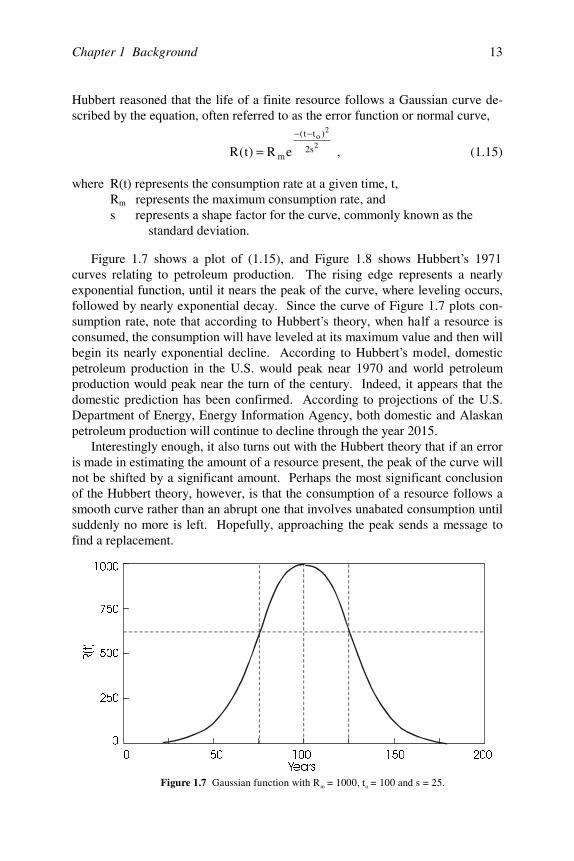
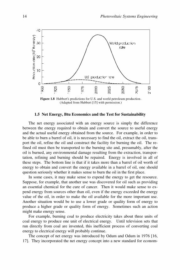
Figure 1.7 shows a plot of (1.15), and Figure 1.8 shows Hubbert’s 1971curves relating to petroleum production. The rising edge represents a nearlyexponential function, until it nears the peak of the curve, where leveling occurs,followed by nearly exponential decay. Since the curve of Figure 1.7 plots con-sumption rate, note that according to Hubbert’s theory, when half a resource isconsumed, the consumption will have leveled at its maximum value and then willbegin its nearly exponential decline. According to Hubbert’s model, domesticpetroleum production in the U.S. would peak near 1970 and world petroleumproduction would peak near the turn of the century. Indeed, it appears that thedomestic prediction has been confirmed. According to projections of the U.S.Department of Energy, Energy Information Agency, both domestic and Alaskanpetroleum production will continue to decline through the year 2015.
Interestingly enough, it also turns out with the Hubbert theory that if an erroris made in estimating the amount of a resource present, the peak of the curve willnot be shifted by a significant amount. Perhaps the most significant conclusionof the Hubbert theory, however, is that the consumption of a resource follows asmooth curve rather than an abrupt one that involves unabated consumption untilsuddenly no more is left. Hopefully, approaching the peak sends a message tofind a replacement.
<HDUV
5W
Figure 1.7 Gaussian function with R = 1000, t = 100 and s = 25.m o
Photovoltaic Systems Engineering14
1.5 Net Energy, Btu Economics and the Test for Sustainability
The net energy associated with an energy source is simply the differencebetween the energy required to obtain and convert the source to useful energyand the actual useful energy obtained from the source. For example, in order tobe able to burn a barrel of oil, it is necessary to find the oil, extract the oil, trans-port the oil, refine the oil and construct the facility for burning the oil. The re-fined oil must then be transported to the burning site and, presumably, after theoil is burned, any environmental damage resulting from the extraction, transpor-tation, refining and burning should be repaired. Energy is involved in all ofthese steps. The bottom line is that if it takes more than a barrel of oil worth ofenergy to obtain and convert the energy available in a barrel of oil, one shouldquestion seriously whether it makes sense to burn the oil in the first place.
In some cases, it may make sense to expend the energy to get the resource.Suppose, for example, that another use was discovered for oil such as providingan essential chemical for the cure of cancer. Then it would make sense to ex-pend energy from sources other than oil, even if the energy exceeded the energyvalue of the oil, in order to make the oil available for the more important use.Another situation would be to use a lower grade or quality form of energy toproduce a higher grade or quality form of energy. Sometimes such an actionmight make energy sense.
For example, burning coal to produce electricity takes about three units ofcoal energy to produce one unit of electrical energy. Until television sets thatrun directly from coal are invented, this inefficient process of converting coalenergy to electrical energy will probably continue.
The concept of net energy was introduced by Odum and Odum in 1976 [16,17]. They incorporated the net energy concept into a new standard for econom-
3URGXFWLRQUDWH%DUUHOV\U
:RUOGSURGXFWLRQUDWH
86SURGXFWLRQUDWH
Figure 1.8 Hubbert’s predictions for U.S. and world petroleum production .(Adapted from Hubbert [15] with permission.)
Chapter 1 Background 15
ics that they felt made better sense than the gold standard. They called it the Btustandard. The Btu standard simply recognizes that everything has an energycontent. Henderson [18] has written extensively on the concept of Btu econom-ics. The reader is encouraged to read Odum and Odum and Henderson during aterm break for enlightening discussions of how the economic system might bechanged to an energy-based standard.
For the purposes of this book, the test for sustainability for an energy sourcewill include two factors. The first will be whether the source is finite. A finitesource is generally termed nonrenewable, while an infinite source is termed re-newable. The second will be whether the source has positive net energy. Thatis, once energy is expended to produce the source, will the source then generatemore energy than was required for its production?
The idea that a source can produce more energy than was used to create thesource may seem inconsistent with the second law of thermodynamics. How-ever, if we allow the use of energy from a very large reservoir as a supply ofenergy to be converted by the source, then the source becomes nearly infinite. Inthe case of the sun, which is expected to survive for another 4 billion years or so[19], we have such a reservoir. Thus, for example, if a photovoltaic cell cangenerate more electrical energy over its lifetime than was expended in its pro-duction and deployment and ultimately in its disposal, including environmentalenergy costs, then the cell would be considered to have positive net energy.
The concept of net energy will be considered in the context of photovoltaiccell production and in discussion of environmental effects of energy sources.
1.6 Direct Conversion of Sunlight to Electricity with Photovoltaics
Becquerel [20] first discovered that sunlight can be converted directly intoelectricity in 1839, when he observed the photogalvanic effect. Then, in 1876,Adams and Day found that selenium has photovoltaic properties. When Planckpostulated the quantum nature of light in 1900, the door was opened for otherscientists to build on this theory. It was in 1930 that Wilson proposed the quan-tum theory of solids, providing a theoretical linkage between the photon and theproperties of solids. Ten years later, Mott and Schottky developed the theory ofthe solid state diode, and in 1949, Bardeen, Brattain and Shockley invented thebipolar transistor. This invention, of course, revolutionized the world of solidstate devices. The first solar cell, developed by Chapin, Fuller and Pearson,followed in 1954. It had an efficiency of 6%. Only four years later, the firstsolar cells were used on the Vanguard I orbiting satellite.
One might wonder why it took so long to develop the photovoltaic cell. Theanswer lies in the difficulty in producing sufficiently pure materials to obtain areasonable level of cell efficiency. Prior to the development of the bipolar tran-sistor and the advent of the space program, there was little impetus for concen-trating on preparing highly pure semiconductor materials. Coal and oil weremeeting the world’s need for electricity and vacuum tubes were meeting the
Photovoltaic Systems Engineering16
needs of the electronics industry. But since vacuum tubes and conventionalpower sources were impractical for space use, solid state gained its foothold.
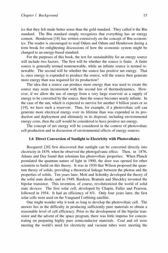
Photovoltaic cells are made of semiconductor materials and are assembledinto modules of approximately 36 cells. This observation is significant, sincethis means the same industry that has, in the past 50 years, progressed from thedevelopment of the bipolar transistor to integrated circuits containing millions oftransistors is also involved in the development of photovoltaic cells. Figure 1.9shows the decline in cost of photovoltaic modules over the past 25 years. Muchof the initial cost reduction has been due to process improvement in the produc-tion of the cells. At this point, the limiting factor is becoming the energy cost ofthe cells. Hence, the challenge of the future will be to reduce the energy contentof the cell production process while maintaining or increasing cell performance,efficiency and reliability.
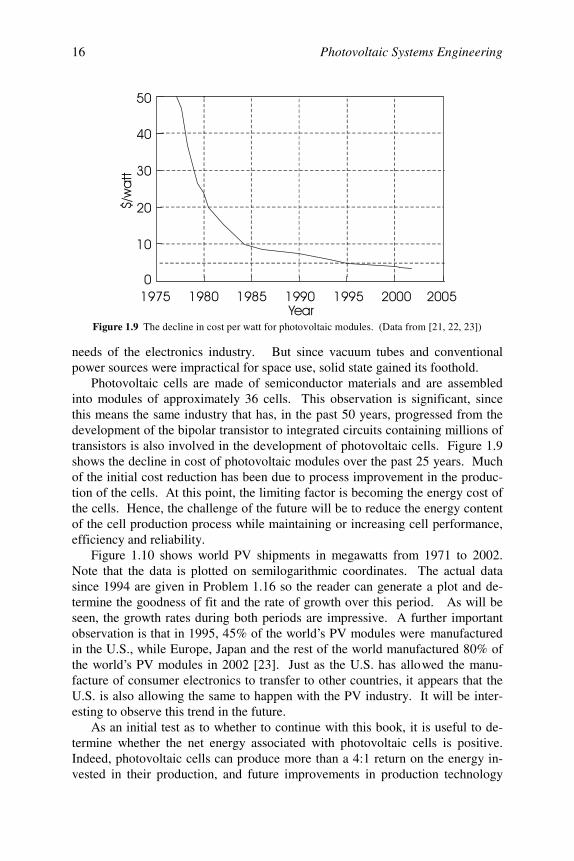
Figure 1.10 shows world PV shipments in megawatts from 1971 to 2002.Note that the data is plotted on semilogarithmic coordinates. The actual datasince 1994 are given in Problem 1.16 so the reader can generate a plot and de-termine the goodness of fit and the rate of growth over this period. As will beseen, the growth rates during both periods are impressive. A further importantobservation is that in 1995, 45% of the world’s PV modules were manufacturedin the U.S., while Europe, Japan and the rest of the world manufactured 80% ofthe world’s PV modules in 2002 [23]. Just as the U.S. has allowed the manu-facture of consumer electronics to transfer to other countries, it appears that theU.S. is also allowing the same to happen with the PV industry. It will be inter-esting to observe this trend in the future.
As an initial test as to whether to continue with this book, it is useful to de-termine whether the net energy associated with photovoltaic cells is positive.Indeed, photovoltaic cells can produce more than a 4:1 return on the energy in-vested in their production, and future improvements in production technology
Figure 1.9 The decline in cost per watt for photovoltaic modules. (Data from [21, 22, 23])
# # # #
!
3
#
4(5
Chapter 1 Background 17
and practice will likely result in exceeding this value. Hence, it appears to beworth investigating this technology in more detail.
Problems 1.1 Prove equation 1.5.
1.2 Calculate the approximate and exact doubling times for annual percentageincreases of 5%, 10%, 15% and 20%.
1.3 The human population of the earth is approximately 6 billion and is in-creasing at approximately 2% per year. The diameter of the earth is ap-proximately 8000 miles and the surface of the earth is approximately two-thirds water. Calculate the population doubling time, then set up a spread-sheet that will show a) the population, b) the number of square feet of landarea per person, and c) the length of the side of a square that will producethe required area per person. Carry out the spreadsheet for 15 doublingtimes, assuming that the rate of population increase remains constant.What conclusions can you draw from this exercise?
1.4 Assume there is enough coal left to last for another 300 years at currentconsumption rates.a. Determine how long the coal will last if its use is increased at a rate of
5% per year.b. If there is enough coal to last for 10,000 years at current consumption
rates, then how long will it last if its use increases by 5% per year?c. Can you predict any other possible consequences if coal burning in-
creases at 5% per year for the short or long term?
Figure 1.10 Worldwide PV shipments, 1971 2002 (Data from [22, 23, 24])−
*
.
5
# # # #

Photovoltaic Systems Engineering18
d. Determine the annual percent reduction in coal consumption to ensurethat coal will last forever, assuming the 300-year lifetime at presentconsumption rates.
1.5 If the half-life of a radioactive isotope is 500 years, how many years will ittake for an amount of the isotope to decay to 1% of its original value?
1.6 If a colony of bacteria lives in a jar and doubles in number every day, andit takes 30 days to fill the jar with bacteria,a. How long does it take for the jar to be half full?b. How long before the bacteria notice they have a problem? (You may
want to pretend you are a bacterium.) c. If on the 30th day, 3 more jars are found, how much longer will the col-
ony be able to continue to multiply at its present rate?
1.7 An enterprising young engineer enters an interesting salary agreement withan employer. She agrees to work for a penny the first day, 2 cents the sec-ond, 4 cents the third, and so on, each day doubling the amount of the pre-vious day. Set up a spreadsheet that will show her daily and cumulativeearnings for her first 30 days of employment.
1.8 Burning a gallon of petroleum produces approximately 25 pounds of car-bon dioxide and burning a ton of coal produces approximately 7000pounds of carbon dioxide.a. If a barrel of petroleum contains 42 gallons, if the world consumes 70
million barrels of petroleum per day and if the atmosphere weighs 14.7pounds per square inch of earth surface area, calculate the weight ofcarbon dioxide generated each year from burning petroleum and com-pare this amount with the weight of the atmosphere.
b. If a total of 14 million tons of coal are burned every day on the earth,calculate the weight of carbon dioxide generated each year from coalburning and compare it with the weight of the atmosphere.
1.9 Assume a world population of 6 billion and a U.S. population of 270 mil-lion.a. Using the data in Figures 1.2–1.4, determine the total world energy
consumption in quads if the rest of the world were to use the same percapita energy as in the U.S.
b. If the energy source mix were to remain the same as the present mix inachieving the scenario of part a, what would be the percentage increasein CO2 emissions?
1.10 Obtain data on worldwide energy consumption by sector from the UnitedStates Department of Energy, Energy Information Administration website.

Chapter 1 Background 19
Plot the data and estimate annual percentage growth rates for the seven re-gions reported and then for the world.
1.11 The following measurements of x(t) are made:
t 0 1 2.3 3.0 4.5 5.2 6.5 8.0x 2.1 8.4 31 65 360 850 3700 20,000
Construct a semilog plot of x(t) either manually or with a computer, anddetermine whether the function appears to have an exponential depend-ence. If so, determine x(t).
1.12 a. What does the area under the Gaussian curve represent?b. Show that 68% of the area under the Gaussian curve lies within one
standard deviation, s, of maximum value of the function.c. What percentage of the area lies within 2s?
1.13 Determine Rm, to and s for the worldwide graph of Figure 1.7.
1.14 Look up actual U. S. and world petroleum production figures and plot themon Hubbert’s curves to compare the actual production with the theoreticalproduction.
1.15 Based on the data of Figure 1.10,a. Estimate the year when PV shipments will reach 1000 MW.b. Estimate the year when PV shipments will reach 10,000 MW.c. Estimate the year when PV shipments will reach 2700 GW.
1.16 Paul Maycock [23, 24] reports the following worldwide PV productionfigures. Plot the data on an Excel graph, establish an equation to representthe data, and then answer the three questions posed in Problem 1.15. Com-pare the results of the two problems.
Year 1994 1995 1996 1997 1998 1999 2000 2001 2002MW 69.4 77.6 88.6 126 155 201 288 391 513
References
[1] Remarks by President William Clinton in Address to the United Nations SpecialSession on Environment and Development, June 26, 1997.
[2] Peña, F. F., U. S. Secretary of Energy, “Remarks on Presid ent Clinton’s Address ofJune 26, 1997,” June 27, 1997.
[3] Bos, E., et al., World Population Projections, 1994–95 , The Johns Hopkins Uni-versity Press, Baltimore, 1994.
[4] Lindley, D., An overview of renewable energy in China, Renewable Energy World,November 1998, 65–69.
[5] Fishbane, P. M., Gasiorowicz, S. and Thornton, S. T., Physics for Scientists andEngineers, 2nd Ed., Prentice Hall, Upper Saddle River, NJ, 1996.

Photovoltaic Systems Engineering20
[6] Annual Energy Review, 2001, U.S. Department of Energy, Energy InformationAdministration, Washington, D.C. (www.eia.doe.gov/emeu/aer).
[7] International Energy Annual 2000: World Overview, U.S. Department of Energy,Energy Information Administration, Washington, D.C. (www.eia.doe.gov/emeu).
[8] World per capita Primary Energy Consumption, U.S. Department of Energy, En-ergy Information Administration, Washington, D.C. (www.eia.doe.gov/emeu).
[9] World Primary Energy Consumption per GDP, U.S. Department of Energy, EnergyInformation Administration, Washington, D.C. (www.eia.doe.gov/emeu)
[10] Malthus, T. R., An Essay on the Principle of Population, as It Affects the FutureImprovement of Society, with Remarks on the Speculations of Mr. Godwin, M.Condorcet, and Other Writers, Printed for J. Johnson in St. Paul’s Church-Yard,London, 1798.
[11] Bahr, H. M., Chadwick, B. A. and Thomas, D. L., Eds., Population, Resources,and the Future: Non-Malthusian Perspectives, Brigham Young University Press,Provo, UT, 1974.
[12] Bloch, S. C., Excel for Engineers and Scientists, 2nd Ed., John Wiley & Sons,Hoboken, N. J., 2003.
[13] Gottfried, B., Spreadsheet Tools for Engineers Using Excel, Including Excel 2002,McGraw-Hill, New York, 2003.
[14] Bartlett, A. A., Forgotten fundamentals of the energy crisis, Am. J. Phys. Vol 46,No 9, September 1978, 876–888.
[15] Hubbert, M. K., The energy resources of the earth, Scientific Am., Vol 225, No 3,September 1971, 60–70.
[16] Odum, H. T. and Odum, E. C., Energy Basis for Man and Nature, McGraw-Hill,New York , 1976.
[17] Odum, H. T. and Odum, E. C., Energy Basis for Man and Nature, 2nd Ed.,McGraw-Hill, New York, 1981.
[18] Henderson, H., The Politics of the Solar Age: Alternatives to Economics, AnchorPress/Doubleday, Garden City, NY, 1981.
[19] Foukal, P., Solar Astrophysics, John Wiley & Sons, New York, 1990.[20] Markvart, T., Ed., Solar Electricity, John Wiley & Sons, Chichester, U.K., 1994.[21] Maycock, P. D., Ed., Photovoltaic News, Vol 18, No 1, January 1999.[22] International Marketing Data and Statistics, 22nd Ed., Euromonitor PIC, London,
1998.[23] Maycock, P. D., The world PV market, production increases 36%, Renewable En-
ergy World, July-August 2002, 147–161.[24] Maycock, P. D., PV News, Vol 22, No 3, March 2003.
Suggested Reading
Aubrecht, G. J., Energy, 2nd Ed., Prentice Hall, Upper Saddle River, NJ, 1995.Kerr, R. A., The next oil crisis looms large and perhaps close, Science, Vol 281,
August 21, 1998, 1128–1131.“President Clinton Announces Million Solar Roofs by 2010,” FEMP Focus,
August/September 1997, 7.Silberberg, M., Chemistry: The Molecular Nature of Matter and Change, Mosby,
St. Louis, 1996.Starke, L., Ed., Vital Signs 1998: The Environmental Trends That Are Shaping Our
Future, W. W. Norton, New York, London, 1998.
21
Chapter 2THE SUN
2.1 Introduction
Optimization of the performance of photovoltaic and other systems that con-vert sunlight into other useful forms of energy is contingent on knowledge of theproperties of sunlight. This chapter provides a synopsis of important solar phe-nomena, including the solar spectrum, atmospheric effects, solar radiation com-ponents, determination of sun position, measurement of solar parameters andpositioning of the solar collector. In this chapter, an attempt is made to quantifythe obvious and, perhaps, some not-so-obvious observations: Why is it lightduring the day and dark at night? Why are there more daylight hours in summerthan in winter? Why is the sun higher in the sky in summer than in winter? Whyare there more summer sunlight hours in northern latitudes than in latitudescloser to the equator? Why does less energy reach the surface of the Earth oncloudy days? Why is it better for a solar collector to face the sun? What hap-pens if a solar collector does not face the sun directly? How much energy isavailable from the sun? Why is the sky blue?
2.2 The Solar Spectrum
The sun provides the energy needed to sustain life in our solar system. Inone hour, the Earth receives enough energy from the sun to meet its energy needsfor nearly a year. In other words, this is about 5000 times the input to theEarth’s energy budget from all other sources. In order to maximize the utiliza-tion of this important energy resource, it is useful to understand some of theproperties of this “ball of fire” in the sky.
The sun is composed of a mixture of gases with a predominance of hydrogen.As the sun converts hydrogen to helium in a massive thermonuclear fusion reac-tion, mass is converted to energy according to Einstein’s famous formula, E =mc2. As a result of this reaction the surface of the sun is maintained at a tem-perature of approximately 5800 K. This energy is radiated away from the sununiformly in all directions, in close agreement with Planck’s blackbody radiationformula
1e
hc2w
kT
hc
52
−
λπ=λ
−
λ (W/m2/unit wavelength in meters), (2.1)
where h = 6.63 × 10⁻³⁴ watt sec2 (Planck’s constant), andk = 1.38 × 10⁻²³ joules/K (Boltzmann’s constant).
Equation 2.1 yields the energy density at the surface of the sun in W/m2/unitwavelength in m. By the time this energy has traveled 150 million km to the
Photovoltaic Systems Engineering22
Earth, the total extraterrestrial energy density decreases to 1367 W/m2 and isoften referred to as the solar constant (see Problem 2.1) [1].
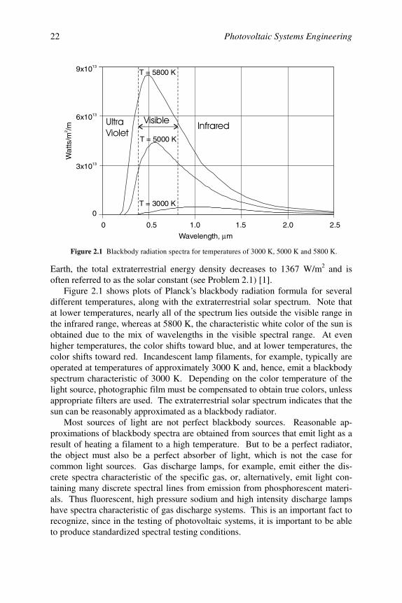
Figure 2.1 shows plots of Planck’s blackbody radiation formula for severaldifferent temperatures, along with the extraterrestrial solar spectrum. Note thatat lower temperatures, nearly all of the spectrum lies outside the visible range inthe infrared range, whereas at 5800 K, the characteristic white color of the sun isobtained due to the mix of wavelengths in the visible spectral range. At evenhigher temperatures, the color shifts toward blue, and at lower temperatures, thecolor shifts toward red. Incandescent lamp filaments, for example, typically areoperated at temperatures of approximately 3000 K and, hence, emit a blackbodyspectrum characteristic of 3000 K. Depending on the color temperature of thelight source, photographic film must be compensated to obtain true colors, unlessappropriate filters are used. The extraterrestrial solar spectrum indicates that thesun can be reasonably approximated as a blackbody radiator.
Most sources of light are not perfect blackbody sources. Reasonable ap-proximations of blackbody spectra are obtained from sources that emit light as aresult of heating a filament to a high temperature. But to be a perfect radiator,the object must also be a perfect absorber of light, which is not the case forcommon light sources. Gas discharge lamps, for example, emit either the dis-crete spectra characteristic of the specific gas, or, alternatively, emit light con-taining many discrete spectral lines from emission from phosphorescent materi-als. Thus fluorescent, high pressure sodium and high intensity discharge lampshave spectra characteristic of gas discharge systems. This is an important fact torecognize, since in the testing of photovoltaic systems, it is important to be ableto produce standardized spectral testing conditions.
0 0.5 1.0 1.5 2.0 2.5
0
3x10¹³
6x10¹³
9x10¹³W
atts
/m/m2
Wavelength, mµ
T = 5800 K
T = 5000 K
T = 3000 K
Figure 2.1 Blackbody radiation spectra for temperatures of 3000 K, 5000 K and 5800 K.
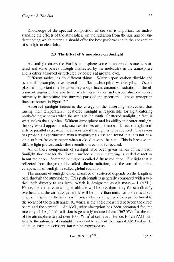
Chapter 2 The Sun 23
Knowledge of the spectral composition of the sun is important for under-standing the effects of the atmosphere on the radiation from the sun and for un-derstanding which materials should offer the best performance in the conversionof sunlight to electricity.
2.3 The Effect of Atmosphere on Sunlight
As sunlight enters the Earth’s atmosphere some is absorbed, some is scat-tered and some passes through unaffected by the molecules in the atmosphereand is either absorbed or reflected by objects at ground level.
Different molecules do different things. Water vapor, carbon dioxide andozone, for example, have several significant absorption wavelengths. Ozoneplays an important role by absorbing a significant amount of radiation in the ul-traviolet region of the spectrum, while water vapor and carbon dioxide absorbprimarily in the visible and infrared parts of the spectrum. These absorptionlines are shown in Figure 2.2.
Absorbed sunlight increases the energy of the absorbing molecules, thusraising their temperature. Scattered sunlight is responsible for light enteringnorth-facing windows when the sun is in the south. Scattered sunlight, in fact, iswhat makes the sky blue. Without atmosphere and its ability to scatter sunlight,the sky would appear black, such as it does on the moon. Direct sunlight con-sists of parallel rays, which are necessary if the light is to be focused. The readerhas probably experimented with a magnifying glass and found that it is not pos-sible to burn holes in paper when a cloud covers the sun. This is because thediffuse light present under these conditions cannot be focused.
All of these components of sunlight have been given names of their own.Sunlight that reaches the Earth’s surface without scattering is called direct orbeam radiation. Scattered sunlight is called diffuse radiation. Sunlight that isreflected from the ground is called albedo radiation, and the sum of all threecomponents of sunlight is called global radiation.
The amount of sunlight either absorbed or scattered depends on the length ofpath through the atmosphere. This path length is generally compared with a ver-tical path directly to sea level, which is designated as air mass = 1 (AM1).Hence, the air mass at a higher altitude will be less than unity for sun directlyoverhead and the air mass generally will be more than unity for nonvertical sunangles. In general, the air mass through which sunlight passes is proportional tothe secant of the zenith angle, θ z, which is the angle measured between the directbeam and the vertical. At AM1, after absorption has been accounted for, theintensity of the global radiation is generally reduced from 1367 W/m2 at the topof the atmosphere to just over 1000 W/m2 at sea level. Hence, for an AM1 pathlength, the intensity of sunlight is reduced to 70% of its original AM0 value. Inequation form, this observation can be expressed as
AM)7.0(1367I = . (2.2)
Photovoltaic Systems Engineering24
This equation is, of course, obvious for AM1. But does it hold for air massesdifferent from unity? According to Meinel and Meinel [2], a better fit to ob-served data is given by
678.0)AM()7.0(1367I = . (2.3)
On the average, over the surface of the Earth, an amount of heat is reradiatedinto space at night that is just equal to the amount absorbed from the sun duringthe day. As long as this steady state condition persists, the average temperatureof the Earth will remain constant. However, if for any reason the amount of heatabsorbed is not equal to the amount reradiated, the planet will either cool downor heat up. This delicate balance can be upset by events such as volcanoes thatfill the atmosphere with fine ash that reflects the sunlight away from the Earth,thus reducing the amount of incident sunlight. The balance can also be upset bygases such as carbon dioxide and methane, which are mostly transparent to shortwavelength (visible) radiation, but more absorbing to long wavelength (infrared)radiation. Since the incident sunlight is dominated by short wavelengths char-acteristic of the 5800 K sun surface temperature, and since the reradiated energyis dominated by long wavelengths characteristic of the Earth surface temperatureof approximately 300 K, these greenhouse gases tend to prevent the Earth fromreradiating heat at night. In order to reach a new balance, it is necessary for theEarth to increase its temperature, since radiation is proportional to T4, where T isthe temperature in K.
The natural compensation mechanism is green plants on land and under wa-ter. Through the process of photosynthesis, they use sunlight and carbon dioxideto produce plant fiber and oxygen, which is released to the atmosphere. Hence,replacement of green plants with concrete and asphalt and adding carbon dioxideto the atmosphere by burning fossil fuels have a combined negative effect on the
Figure 2.2 AM 1 solar spectrum after atmospheric absorption effects, including plots ofextraterrestrial blackbody spectrum plus cumulative incident energy vs. wavelength.
µ
!!"#
$%&' (
"#
Chapter 2 The Sun 25
stability of the concentration of carbon dioxide in the atmosphere. Globalwarming has been discussed extensively in other literature, some of which islisted in the chapter references.
2.4 Insolation Specifics
2.4.1 Introduction
Nearly everyone has noticed that the sun shines longer in the summer than inthe winter. Nearly everyone also knows that the Sahara Desert receives moresunshine than does London. Another obvious observation is that cloudy placesreceive less sunlight than sunny places. It may be less evident, however, that thehours of sunlight over a year are the same for every point on the Earth, providedthat only the hours between sunrise and sunset are counted, regardless of cloudcover. Those regions of the Earth closer to the poles that have long winter nightsalso have long summer days. However, since the sun, on the average, is lowerin the sky in the polar regions than in the tropics, sunlight must traverse greaterair mass in the polar regions than in the tropics. As a result, polar sunlight car-ries less energy to the surface than does tropical sunlight. Not surprisingly, thepolar regions are colder than the tropics.
In this section, quantitative formulas will be presented that will enable thereader to determine exactly how long the sun shines in any particular place onany particular day, and to determine how much sunlight can be expected, on theaverage, during any month at various locations. Means will also be presented fordetermining the position of the sun at any time on any day at any location. Fi-nally, the effects of varying the orientation of a photovoltaic array on the powerand energy produced by the array will be discussed.
Irradiance is the measure of the power density of sunlight and is measuredin W/m2. Irradiance is thus an instantaneous quantity. The solar constant forEarth is the irradiance received by the Earth from the sun at the top of the at-mosphere, i.e., at AM0, and is equal to 1367 W/m2. After passing through theatmosphere with a path length of AM1, the irradiance is reduced to approxi-mately 1000 W/m2, and has a modified spectral content due to atmospheric ab-sorption. The irradiance for AM1.5 is accepted as the standard calibration spec-trum for photovoltaic cells.
Irradiation is the measure of energy density of sunlight and is measured inkWh/m2. Since energy is power integrated over time, irradiation is the integralof irradiance. Normally, the time frame for integration is one day, which, ofcourse, means during daylight hours.
Irradiation is often expressed as peak sun hours (psh). The psh is simply thelength of time in hours at an irradiance level of 1 kW/m2 needed to produce thedaily irradiation obtained from integration of irradiance over all daylight hours.
Irradiance and irradiation both apply to all components of sunlight. Hence,at a given time, or for a given day, these quantities will depend on location,
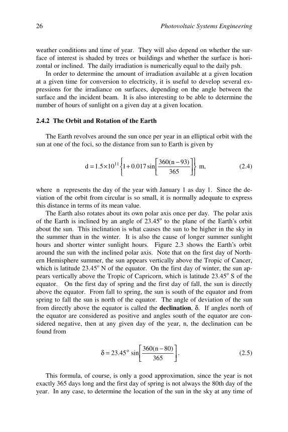
Photovoltaic Systems Engineering26
weather conditions and time of year. They will also depend on whether the sur-face of interest is shaded by trees or buildings and whether the surface is hori-zontal or inclined. The daily irradiation is numerically equal to the daily psh.
In order to determine the amount of irradiation available at a given locationat a given time for conversion to electricity, it is useful to develop several ex-pressions for the irradiance on surfaces, depending on the angle between thesurface and the incident beam. It is also interesting to be able to determine thenumber of hours of sunlight on a given day at a given location.
2.4.2 The Orbit and Rotation of the Earth
The Earth revolves around the sun once per year in an elliptical orbit with thesun at one of the foci, so the distance from sun to Earth is given by
−+×=
365
)93n(360sin017.01105.1d 11 m, (2.4)
where n represents the day of the year with January 1 as day 1. Since the de-viation of the orbit from circular is so small, it is normally adequate to expressthis distance in terms of its mean value.
The Earth also rotates about its own polar axis once per day. The polar axisof the Earth is inclined by an angle of 23.45o to the plane of the Earth’s orbitabout the sun. This inclination is what causes the sun to be higher in the sky inthe summer than in the winter. It is also the cause of longer summer sunlighthours and shorter winter sunlight hours. Figure 2.3 shows the Earth’s orbitaround the sun with the inclined polar axis. Note that on the first day of North-ern Hemisphere summer, the sun appears vertically above the Tropic of Cancer,which is latitude 23.45o N of the equator. On the first day of winter, the sun ap-pears vertically above the Tropic of Capricorn, which is latitude 23.45o S of theequator. On the first day of spring and the first day of fall, the sun is directlyabove the equator. From fall to spring, the sun is south of the equator and fromspring to fall the sun is north of the equator. The angle of deviation of the sunfrom directly above the equator is called the declination, δ . If angles north ofthe equator are considered as positive and angles south of the equator are con-sidered negative, then at any given day of the year, n, the declination can befound from
−
=δ365
)80n(360sin45.23 o . (2.5)
This formula, of course, is only a good approximation, since the year is notexactly 365 days long and the first day of spring is not always the 80th day of theyear. In any case, to determine the location of the sun in the sky at any time of
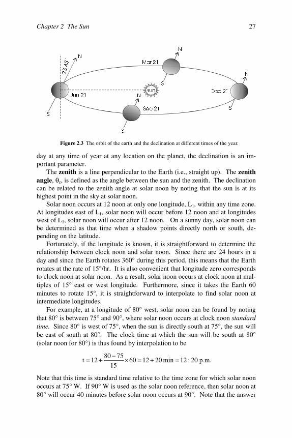
Chapter 2 The Sun 27
day at any time of year at any location on the planet, the declination is an im-portant parameter.
The zenith is a line perpendicular to the Earth (i.e., straight up). The zenithangle, θ z, is defined as the angle between the sun and the zenith. The declinationcan be related to the zenith angle at solar noon by noting that the sun is at itshighest point in the sky at solar noon.
Solar noon occurs at 12 noon at only one longitude, L1, within any time zone.At longitudes east of L1, solar noon will occur before 12 noon and at longitudeswest of L1, solar noon will occur after 12 noon. On a sunny day, solar noon canbe determined as that time when a shadow points directly north or south, de-pending on the latitude.
Fortunately, if the longitude is known, it is straightforward to determine therelationship between clock noon and solar noon. Since there are 24 hours in aday and since the Earth rotates 360° during this period, this means that the Earthrotates at the rate of 15°/hr. It is also convenient that longitude zero correspondsto clock noon at solar noon. As a result, solar noon occurs at clock noon at mul-tiples of 15° east or west longitude. Furthermore, since it takes the Earth 60minutes to rotate 15°, it is straightforward to interpolate to find solar noon atintermediate longitudes.
For example, at a longitude of 80° west, solar noon can be found by notingthat 80° is between 75° and 90°, where solar noon occurs at clock noon standardtime. Since 80° is west of 75°, when the sun is directly south at 75°, the sun willbe east of south at 80°. The clock time at which the sun will be south at 80°(solar noon for 80°) is thus found by interpolation to be
20:12min20126015
758012t =+=×−+= p.m.
Note that this time is standard time relative to the time zone for which solar noonoccurs at 75° W. If 90° W is used as the solar noon reference, then solar noon at80° will occur 40 minutes before solar noon occurs at 90°. Note that the answer
1
6
1
6
1
6
1
6
VXQ
R
'HF-XQ
0DU
6HS
Figure 2.3 The orbit of the earth and the declination at different times of the year.
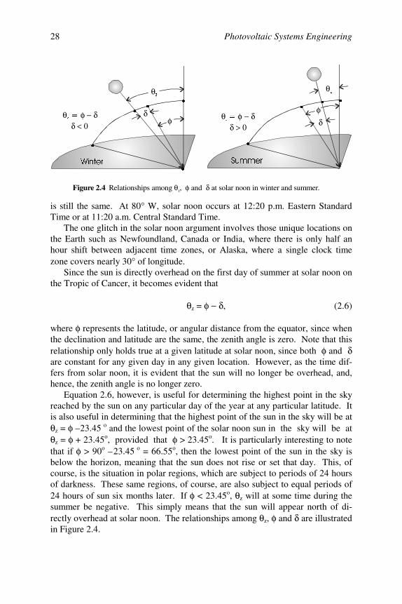
Photovoltaic Systems Engineering28
is still the same. At 80° W, solar noon occurs at 12:20 p.m. Eastern StandardTime or at 11:20 a.m. Central Standard Time.
The one glitch in the solar noon argument involves those unique locations onthe Earth such as Newfoundland, Canada or India, where there is only half anhour shift between adjacent time zones, or Alaska, where a single clock timezone covers nearly 30° of longitude.
Since the sun is directly overhead on the first day of summer at solar noon onthe Tropic of Cancer, it becomes evident that
θ z = φ − δ , (2.6)
where φ represents the latitude, or angular distance from the equator, since whenthe declination and latitude are the same, the zenith angle is zero. Note that thisrelationship only holds true at a given latitude at solar noon, since both φ and δare constant for any given day in any given location. However, as the time dif-fers from solar noon, it is evident that the sun will no longer be overhead, and,hence, the zenith angle is no longer zero.
Equation 2.6, however, is useful for determining the highest point in the skyreached by the sun on any particular day of the year at any particular latitude. Itis also useful in determining that the highest point of the sun in the sky will be atθ z = φ – 23.45 o and the lowest point of the solar noon sun in the sky will be atθ z = φ + 23.45o, provided that φ > 23.45o. It is particularly interesting to notethat if φ > 90o – 23.45 o = 66.55o, then the lowest point of the sun in the sky isbelow the horizon, meaning that the sun does not rise or set that day. This, ofcourse, is the situation in polar regions, which are subject to periods of 24 hoursof darkness. These same regions, of course, are also subject to equal periods of24 hours of sun six months later. If φ < 23.45o, θ z will at some time during thesummer be negative. This simply means that the sun will appear north of di-rectly overhead at solar noon. The relationships among θ z, φ and δ are illustratedin Figure 2.4.
:LQWHU 6XPPHU
θ ]
θ φ − δ δ < 0
] δ δ
θ φ − δ δ > 0
]
θ ]
φφ
oo
o
o
o
o
o
o
o
Figure 2.4 Relationships among , and at solar noon in winter and summer.θ φ δ z
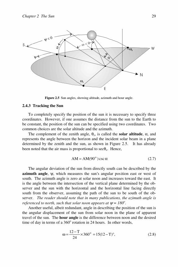
Chapter 2 The Sun 29
2.4.3 Tracking the Sun
To completely specify the position of the sun it is necessary to specify threecoordinates. However, if one assumes the distance from the sun to the Earth tobe constant, the position of the sun can be specified using two coordinates. Twocommon choices are the solar altitude and the azimuth.
The complement of the zenith angle, θ z, is called the solar altitude, α , andrepresents the angle between the horizon and the incident solar beam in a planedetermined by the zenith and the sun, as shown in Figure 2.5. It has alreadybeen noted that the air mass is proportional to secθ z. Hence,
α= csc)90(AMAM o (2.7)
The angular deviation of the sun from directly south can be described by theazimuth angle, ψ , which measures the sun’s angular position east or west ofsouth. The azimuth angle is zero at solar noon and increases toward the east. Itis the angle between the intersection of the vertical plane determined by the ob-server and the sun with the horizontal and the horizontal line facing directlysouth from the observer, assuming the path of the sun to be south of the ob-server. The reader should note that in many publications, the azimuth angle isreferenced to north, such that solar noon appears at ψ = 180o.
Another useful, albeit redundant, angle in describing the position of the sun isthe angular displacement of the sun from solar noon in the plane of apparenttravel of the sun. The hour angle is the difference between noon and the desiredtime of day in terms of a 360o rotation in 24 hours. In other words,
,)T12(1536024
T12 o °−=×−=ω (2.8)
)
$
ψ < 0
α
*
ψω
ωV
−ωV
Figure 2.5 Sun angles, showing altitude, azimuth and hour angle.
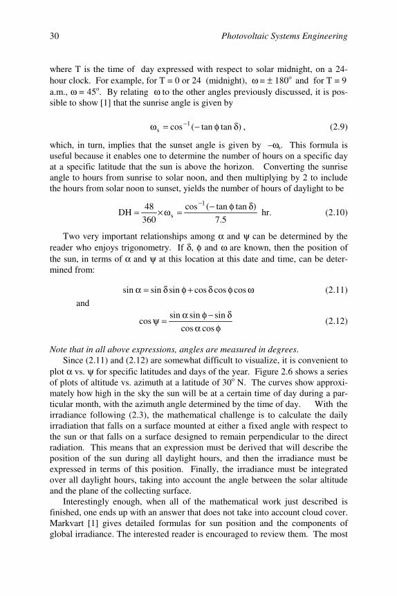
Photovoltaic Systems Engineering30
where T is the time of day expressed with respect to solar midnight, on a 24-hour clock. For example, for T = 0 or 24 (midnight), ω = ± 180o and for T = 9a.m., ω = 45o. By relating ω to the other angles previously discussed, it is pos-sible to show [1] that the sunrise angle is given by
)tantan(cos 1s δφ−=ω − , (2.9)
which, in turn, implies that the sunset angle is given by – ω s. This formula isuseful because it enables one to determine the number of hours on a specific dayat a specific latitude that the sun is above the horizon. Converting the sunriseangle to hours from sunrise to solar noon, and then multiplying by 2 to includethe hours from solar noon to sunset, yields the number of hours of daylight to be
5.7
)tantan(cos
360
48DH
1
sδφ−=ω×=
− hr. (2.10)
Two very important relationships among α and ψ can be determined by thereader who enjoys trigonometry. If δ , φ and ω are known, then the position ofthe sun, in terms of α and ψ at this location at this date and time, can be deter-mined from:
ωφδ+φδ=α coscoscossinsinsin (2.11)
and
φαδ−φα=ψ
coscos
sinsinsincos (2.12)
Note that in all above expressions, angles are measured in degrees.Since (2.11) and (2.12) are somewhat difficult to visualize, it is convenient to
plot α vs. ψ for specific latitudes and days of the year. Figure 2.6 shows a seriesof plots of altitude vs. azimuth at a latitude of 30o N. The curves show approxi-mately how high in the sky the sun will be at a certain time of day during a par-ticular month, with the azimuth angle determined by the time of day. With theirradiance following (2.3), the mathematical challenge is to calculate the dailyirradiation that falls on a surface mounted at either a fixed angle with respect tothe sun or that falls on a surface designed to remain perpendicular to the directradiation. This means that an expression must be derived that will describe theposition of the sun during all daylight hours, and then the irradiance must beexpressed in terms of this position. Finally, the irradiance must be integratedover all daylight hours, taking into account the angle between the solar altitudeand the plane of the collecting surface.
Interestingly enough, when all of the mathematical work just described isfinished, one ends up with an answer that does not take into account cloud cover.Markvart [1] gives detailed formulas for sun position and the components ofglobal irradiance. The interested reader is encouraged to review them. The most
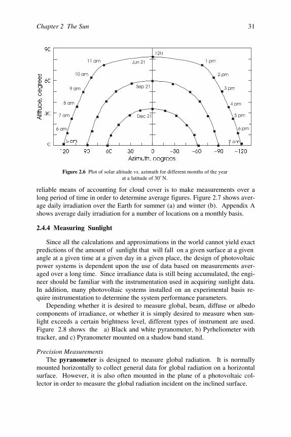
Chapter 2 The Sun 31
reliable means of accounting for cloud cover is to make measurements over along period of time in order to determine average figures. Figure 2.7 shows aver-age daily irradiation over the Earth for summer (a) and winter (b). Appendix Ashows average daily irradiation for a number of locations on a monthly basis.
2.4.4 Measuring Sunlight
Since all the calculations and approximations in the world cannot yield exactpredictions of the amount of sunlight that will fall on a given surface at a givenangle at a given time at a given day in a given place, the design of photovoltaicpower systems is dependent upon the use of data based on measurements aver-aged over a long time. Since irradiance data is still being accumulated, the engi-neer should be familiar with the instrumentation used in acquiring sunlight data.In addition, many photovoltaic systems installed on an experimental basis re-quire instrumentation to determine the system performance parameters.
Depending whether it is desired to measure global, beam, diffuse or albedocomponents of irradiance, or whether it is simply desired to measure when sun-light exceeds a certain brightness level, different types of instrument are used.Figure 2.8 shows the a) Black and white pyranometer, b) Pyrheliometer withtracker, and c) Pyranometer mounted on a shadow band stand.
Precision MeasurementsThe pyranometer is designed to measure global radiation. It is normally
mounted horizontally to collect general data for global radiation on a horizontalsurface. However, it is also often mounted in the plane of a photovoltaic col-lector in order to measure the global radiation incident on the inclined surface.
Figure 2.6 Plot of solar altitude vs. azimuth for different months of the yearat a latitude of 30 N.o
− − − −$]LPXWKGHJUHHV
$OWLWXGHGHJUHHV
DP SP
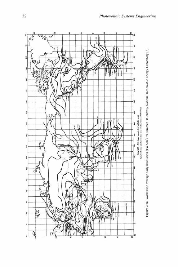
Photovoltaic Systems Engineering32
Fig
ure
2.7a
Wor
ldw
ide
aver
age
daily
irra
diat
ion
(kW
h/m
) fo
r su
mm
er.
(Cou
rtes
y N
atio
nal R
enew
able
Ene
rgy
Lab
orat
ory
[3].
2
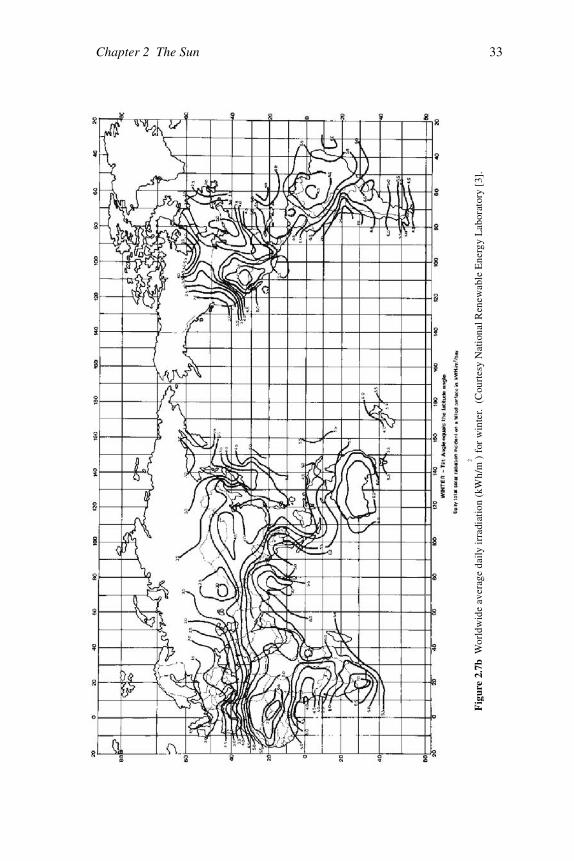
Chapter 2 The Sun 33
Fig
ure
2.7b
Wor
ldw
ide
aver
age
daily
irra
diat
ion
(kW
h/m
) fo
r w
inte
r. (
Cou
rtes
y N
atio
nal R
enew
able
Ene
rgy
Lab
orat
ory
[3].
2
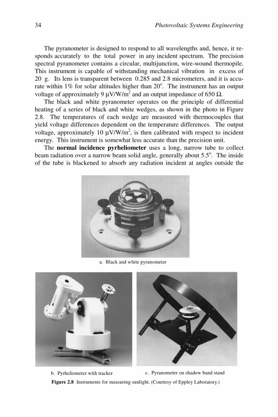
Photovoltaic Systems Engineering34
The pyranometer is designed to respond to all wavelengths and, hence, it re-sponds accurately to the total power in any incident spectrum. The precisionspectral pyranometer contains a circular, multijunction, wire-wound thermopile.This instrument is capable of withstanding mechanical vibration in excess of20 g. Its lens is transparent between 0.285 and 2.8 micrometers, and it is accu-rate within 1% for solar altitudes higher than 20o. The instrument has an outputvoltage of approximately 9 µ V/W/m2 and an output impedance of 650 Ω .
The black and white pyranometer operates on the principle of differentialheating of a series of black and white wedges, as shown in the photo in Figure2.8. The temperatures of each wedge are measured with thermocouples thatyield voltage differences dependent on the temperature differences. The outputvoltage, approximately 10 µ V/W/m2, is then calibrated with respect to incidentenergy. This instrument is somewhat less accurate than the precision unit.
The normal incidence pyrheliometer uses a long, narrow tube to collectbeam radiation over a narrow beam solid angle, generally about 5.5o. The insideof the tube is blackened to absorb any radiation incident at angles outside the
a. Black and white pyranometer
b. Pyrheliometer with tracker c. Pyranometer on shadow band stand
Figure 2.8 Instruments for measuring sunlight. (Courtesy of Eppley Laboratory.)
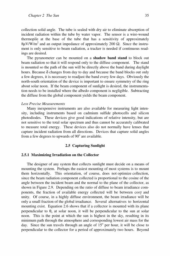
Chapter 2 The Sun 35
collection solid angle. The tube is sealed with dry air to eliminate absorption ofincident radiation within the tube by water vapor. The sensor is a wire-woundthermopile at the base of the tube that has a sensitivity of approximately8 µ V/W/m2 and an output impedance of approximately 200 Ω . Since the instru-ment is only sensitive to beam radiation, a tracker is needed if continuous read-ings are desired.
The pyranometer can be mounted on a shadow band stand to block outbeam radiation so that it will respond only to the diffuse component. The standis mounted so the path of the sun will be directly above the band during daylighthours. Because δ changes from day to day and because the band blocks out onlya few degrees, it is necessary to readjust the band every few days. Obviously thenorth-south orientation of the device is important to ensure symmetry of the ringabout solar noon. If the beam component of sunlight is desired, the instrumenta-tion needs to be installed where the albedo component is negligible. Subtractingthe diffuse from the global component yields the beam component.
Less Precise MeasurementsMany inexpensive instruments are also available for measuring light inten-
sity, including instruments based on cadmium sulfide photocells and siliconphotodiodes. These devices give good indications of relative intensity, but arenot sensitive to the total solar spectrum and thus cannot be accurately calibratedto measure total energy. These devices also do not normally have lenses thatcapture incident radiation from all directions. Devices that capture solid anglesfrom a few degrees to upwards of 90o are available.
2.5 Capturing Sunlight
2.5.1 Maximizing Irradiation on the Collector
The designer of any system that collects sunlight must decide on a means ofmounting the system. Perhaps the easiest mounting of most systems is to mountthem horizontally. This orientation, of course, does not optimize collection,since the beam radiation component collected is proportional to the cosine of theangle between the incident beam and the normal to the plane of the collector, asshown in Figure 2.9. Depending on the ratio of diffuse to beam irradiance com-ponents, the fraction of available energy collected will be between cosγ andunity. Of course, in a highly diffuse environment, the beam irradiance will beonly a small fraction of the global irradiance. Several alternatives to horizontalmounting exist. Equation 2.6 shows that if a collector is mounted with its planeperpendicular to θ z at solar noon, it will be perpendicular to the sun at solarnoon. This is the point at which the sun is highest in the sky, resulting in itsminimum path through the atmosphere and corresponding lowest air mass for theday. Since the sun travels through an angle of 15o per hour, it will be close toperpendicular to the collector for a period of approximately two hours. Beyond
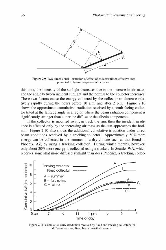
Photovoltaic Systems Engineering36
this time, the intensity of the sunlight decreases due to the increase in air mass,and the angle between incident sunlight and the normal to the collector increases.These two factors cause the energy collected by the collector to decrease rela-tively rapidly during the hours before 10 a.m. and after 2 p.m. Figure 2.10shows the approximate cumulative irradiation received by a south-facing collec-tor tilted at the latitude angle in a region where the beam radiation component issignificantly stronger than either the diffuse or the albedo components.
If the collector is mounted so it can track the sun, then the incident irradi-ance is affected only by the increasing air mass as the sun approaches the hori-zon. Figure 2.10 also shows the additional cumulative irradiation under directbeam conditions received by a tracking collector. Approximately 50% moreenergy can be collected in the summer in a dry climate such as that found inPhoenix, AZ, by using a tracking collector. During winter months, however,only about 20% more energy is collected using a tracker. In Seattle, WA, whichreceives somewhat more diffused sunlight than does Phoenix, a tracking collec-
γ
γ
G
Figure 2.9 Two-dimensional illustration of effect of collector tilt on effective areapresented to beam component of radiation.
!
"
#
$
%
!
&
'(
)*
Figure 2.10 Cumulative daily irradiation received by fixed and tracking collectors fordifferent seasons, direct beam contribution only.
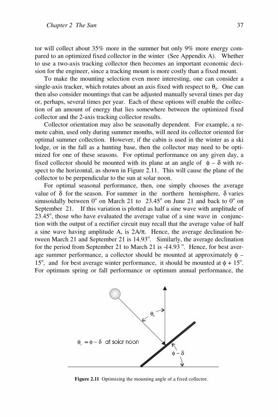
Chapter 2 The Sun 37
tor will collect about 35% more in the summer but only 9% more energy com-pared to an optimized fixed collector in the winter (See Appendix A). Whetherto use a two-axis tracking collector then becomes an important economic deci-sion for the engineer, since a tracking mount is more costly than a fixed mount.
To make the mounting selection even more interesting, one can consider asingle-axis tracker, which rotates about an axis fixed with respect to θ z. One canthen also consider mountings that can be adjusted manually several times per dayor, perhaps, several times per year. Each of these options will enable the collec-tion of an amount of energy that lies somewhere between the optimized fixedcollector and the 2-axis tracking collector results.
Collector orientation may also be seasonally dependent. For example, a re-mote cabin, used only during summer months, will need its collector oriented foroptimal summer collection. However, if the cabin is used in the winter as a skilodge, or in the fall as a hunting base, then the collector may need to be opti-mized for one of these seasons. For optimal performance on any given day, afixed collector should be mounted with its plane at an angle of φ – δ with re-spect to the horizontal, as shown in Figure 2.11. This will cause the plane of thecollector to be perpendicular to the sun at solar noon.
For optimal seasonal performance, then, one simply chooses the averagevalue of δ for the season. For summer in the northern hemisphere, δ variessinusoidally between 0o on March 21 to 23.45o on June 21 and back to 0o onSeptember 21. If this variation is plotted as half a sine wave with amplitude of23.45o, those who have evaluated the average value of a sine wave in conjunc-tion with the output of a rectifier circuit may recall that the average value of halfa sine wave having amplitude A, is 2A/π . Hence, the average declination be-tween March 21 and September 21 is 14.93o. Similarly, the average declinationfor the period from September 21 to March 21 is –14.93 o. Hence, for best aver-age summer performance, a collector should be mounted at approximately φ –15o, and for best average winter performance, it should be mounted at φ + 15o.For optimum spring or fall performance or optimum annual performance, the
θ]
θ]
φ − δ
φ − δ DWVRODUQRRQ
Figure 2.11 Optimizing the mounting angle of a fixed collector.

Photovoltaic Systems Engineering38
collector should be mounted at about 0.9 φ o. Since normally it is acceptable toorient a collector for optimal seasonal or, perhaps, annual performance, manytables of irradiation on collectors are available for collector tilts of either φ , φ +15o , or φ – 15 o at various locations on the globe. Examples of these tables ascompiled by the National Renewable Energy Laboratory are presented in Ap-pendix A. Figure 2.12 shows how monthly performance depends on collector tiltangle. Different locations will show different relative monthly performance,depending on local weather seasonal behavior.
2.5.2 Shading
Even a small amount of shade on a PV module can significantly reduce themodule output current. It is thus of paramount importance to select a site for aPV system where the PV array will remain unshaded for as much of the day aspossible. This is easy if there are no objects that might shade the array, but it isprobably more likely that a site will have objects nearby that shade the array atsome time of the day on some day of the year. The PV system designer mustthus be able to use her knowledge of sun position to determine the times at whicha PV array might be shaded.
Figure 2.13 shows a device that incorporates plots of altitude vs. azimuth forselected latitudes. The device is used at the proposed site to determine when thearray will be shaded by observing the position of reflected objects on the screenof the device. By sketching the outlines of shading objects on the screen withthe device at the proposed location of the collector, the user can then determinewhen the collector will be shaded. For the example in Figure 2.13, the collectorwill be free of shade during May, June, July and August. In September, the col-lector will be unshaded between about 9:15 a.m. and 3:15 p.m. sun time, while inNovember, December and January, the collector is shaded most of the day ex-cept for a short period around 1 p.m. sun time. This proposed collector locationis thus acceptable if the collector is to be used only during the summer months.
5HODWLYHHQHUJ\SURGXFWLRQ
-DQ
)HE
0DU
$SU
0D\
-XQ
-XO
$XJ
6HS
2FW
1RY
'HF
/DWLWXGH
/DWLWXGH − R
/DWLWXGHR
Figure 2.12 Monthly collector performance as a function of collector tilt angle.
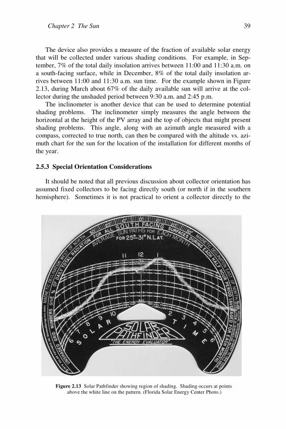
Chapter 2 The Sun 39
The device also provides a measure of the fraction of available solar energythat will be collected under various shading conditions. For example, in Sep-tember, 7% of the total daily insolation arrives between 11:00 and 11:30 a.m. ona south-facing surface, while in December, 8% of the total daily insolation ar-rives between 11:00 and 11:30 a.m. sun time. For the example shown in Figure2.13, during March about 67% of the daily available sun will arrive at the col-lector during the unshaded period between 9:30 a.m. and 2:45 p.m.
The inclinometer is another device that can be used to determine potentialshading problems. The inclinometer simply measures the angle between thehorizontal at the height of the PV array and the top of objects that might presentshading problems. This angle, along with an azimuth angle measured with acompass, corrected to true north, can then be compared with the altitude vs. azi-muth chart for the sun for the location of the installation for different months ofthe year.
2.5.3 Special Orientation Considerations
It should be noted that all previous discussion about collector orientation hasassumed fixed collectors to be facing directly south (or north if in the southernhemisphere). Sometimes it is not practical to orient a collector directly to the
Figure 2.13 Solar Pathfinder showing region of shading. Shading occurs at points above the white line on the pattern. (Florida Solar Energy Center Photo.)
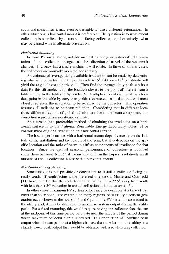
Photovoltaic Systems Engineering40
south and sometimes it may even be desirable to use a different orientation. Inother situations, a horizontal mount is preferable. The question is to what extentcollection is sacrificed by a non-south facing collector, or, alternatively, whatmay be gained with an alternate orientation.
Horizontal MountingIn some PV installations, notably on floating buoys or watercraft, the orien-
tation of the collector changes as the direction of travel of the watercraftchanges. If a buoy has a single anchor, it will rotate. In these or similar cases,the collectors are normally mounted horizontally.
An estimate of average daily available irradiation can be made by determin-ing whether a collector mounting of latitude + 15o, latitude – 15 o or latitude willyield the angle closest to horizontal. Then find the average daily peak sun hour table similar to the tables in Appendix A. Multiplication of each peak sun hourdata point in the table by closely represent the irradiation to be received by the collector. This operationassumes all radiation to be beam radiation. Considering that in different loca-tions, different fractions of global radiation are due to the beam component, thiscorrection represents a worst-case estimate.
An alternate (and preferable) method of obtaining the irradiation on a hori-zontal surface is to use National Renewable Energy Laboratory tables [3] orcontour maps of global irradiation on a horizontal surface.
The loss in performance with a horizontal mount depends mostly on the lati-tude of the installation and the season of the year, but also depends on the spe-cific location and the ratio of beam to diffuse components of irradiance for thatlocation. Since the optimal seasonal performance of collectors is obtainedsomewhere between φ ± 15o, if the installation is in the tropics, a relatively smallamount of annual collection is lost with a horizontal mount.
Non-South Facing MountingSometimes it is not possible or convenient to install a collector facing di-
rectly south. If south-facing is the preferred orientation, Morse and Czarnecki[11] have reported that the collector can be facing up to 22.5o away from southwith less than a 2% reduction in annual collection at latitudes up to 45o.
In other cases, maximum PV system output may be desirable at a time of dayother than solar noon. For example, in many regions, peak utility electrical gen-eration occurs between the hours of 3 and 6 p.m. If a PV system is connected tothe utility grid, it may be desirable to maximize system output during the utilitypeak. For a fixed mounting, this would require having the collector face the sunat the midpoint of this time period on a date near the middle of the period duringwhich maximum collector output is desired. This orientation will produce peakoutput when the sun path is at a higher air mass than at solar noon, resulting in aslightly lower peak output than would be obtained with a south-facing collector.
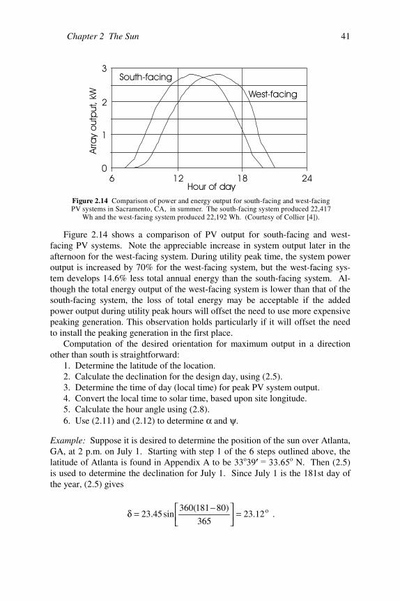
Chapter 2 The Sun 41
Figure 2.14 shows a comparison of PV output for south-facing and west-facing PV systems. Note the appreciable increase in system output later in theafternoon for the west-facing system. During utility peak time, the system poweroutput is increased by 70% for the west-facing system, but the west-facing sys-tem develops 14.6% less total annual energy than the south-facing system. Al-though the total energy output of the west-facing system is lower than that of thesouth-facing system, the loss of total energy may be acceptable if the addedpower output during utility peak hours will offset the need to use more expensivepeaking generation. This observation holds particularly if it will offset the needto install the peaking generation in the first place.
Computation of the desired orientation for maximum output in a directionother than south is straightforward:
1. Determine the latitude of the location.2. Calculate the declination for the design day, using (2.5).3. Determine the time of day (local time) for peak PV system output.4. Convert the local time to solar time, based upon site longitude.5. Calculate the hour angle using (2.8).6. Use (2.11) and (2.12) to determine α and ψ .
Example: Suppose it is desired to determine the position of the sun over Atlanta,GA, at 2 p.m. on July 1. Starting with step 1 of the 6 steps outlined above, thelatitude of Atlanta is found in Appendix A to be 33o39 o N. Then (2.5)is used to determine the declination for July 1. Since July 1 is the 181st day ofthe year, (2.5) gives
o12.23365
)80181(360sin45.23 =
−
=δ .
Figure 2.14 Comparison of power and energy output for south-facing and west-facingPV systems in Sacramento, CA, in summer. The south-facing system produced 22,417
Wh and the west-facing system produced 22,192 Wh. (Courtesy of Collier [4]).
$ " % "#+ &
& (
!
"
(,
- ),
Photovoltaic Systems Engineering42
With 2 p.m. local time (Eastern Daylight Time) at the longitude of Atlanta(84°36 °W) as the time of day for peak system output, the solar timeis found to be 1 p.m. (Eastern Standard Time) plus an additional
4.386015
756.84t =×−= minutes,
or 1:38 p.m.
Next, substituting the solar time in (2.8) yields the hour angle as
oo 60.24)360(24
64.1312 −=−=ω .
The solar altitude is next found from (2.11) with the result
cos65.33cos12.23cos65.33sin12.23sinsin oooo +=α (–24.6 o) = 0.9161.
Next, the azimuth is found from (2.12) to be
3445.065.33cos]9161.0cos[sin
12.23sin65.33sin9161.0cos
o1
oo
=−=ψ−
.
–1 0.9161 = 66.36o –1 0.3445 = 69.85o.
Problems
2.1 Show that, for a surface temperature of 5800 K, the sun will deliver 1367W/m2 to the Earth. This requires integration of the blackbody radiationformula over all wavelengths to determine the total available energy at thesurface of the sun in W/m2. Numerical integration is recommended. Becareful to note the range of wavelengths that contribute the most to thespectrum. Then note that the energy density decreases as the square of thedistance from the source, similar to the behavior of an electric field ema-nating from a point source. The diameter of the sun is 1.393 × 10⁹ m, andthe mean distance from sun to Earth is 1.5 × 10¹¹ m.
Chapter 2 The Sun 43
2.2 If the diameter of the sun is 1.393 × 10⁹ m, and if the average density of thesun is approximately 1.4 × the density of water, and if 2 × 10¹⁹ kg/yr of hy-drogen is consumed by fusion, how long will it take for the sun to consume25% of its mass in the fusion process?
2.3 Calculate the zenith angles needed to produce AM 1.5 and AM 2.0 if AM1.0 occurs at zero degrees.
2.4 Calculate the zenith angle at solar noon at a latitude of 40o north on May 1.
2.5 Calculate the number of hours the sun was above the horizon on yourbirthday at your birthplace.
2.6 Calculate the irradiance of sunlight for AM 1.5 and for AM 2.0, assumingno cloud cover, using (2.2) and (2.3). Then write a computer program thatwill plot irradiance vs. AM for 1 ≤ AM ≤ 10 for each equation.
2.7 Assume no cloud cover, and, hence, that the solar irradiance is predomi-nantly a beam component. If a nontracking collector is perpendicular tothe incident radiation at solar noon, estimate the irradiance on the collectorat 1, 2, 3, 4, 5 and 6 hours past solar noon, taking into account air mass andcollector orientation. Then estimate the total daily irradiation on the col-lector in kWh. Assume AM 1.0 at solar noon and a latitude of 20° N.
2.8 Write a computer program using Matlab, Excel or something similar thatwill plot solar altitude vs. azimuth. Plot sets of curves similar to Figure 2.6for the months of March, June, September and December for Denver, CO,Mexico City, Mexico, and Fairbanks, AK.
2.9 Write a computer program that will generate a plot of solar altitude vs.azimuth for the 12 months of the year for your home town. It would benice if each curve would have time-of-day indicators.
2.10 Calculate the time of day at which solar noon occurs at your longitude.Then compare the north indicated by a compass with the north indicated bya shadow at solar noon and estimate the error in the compass reading.
2.11 Noting the dependence of air mass on θ z,a. Generate a table that shows α , ψ and I (using 2.3) vs. time for a latitude
of your choice on a day of your choice.b. Assuming a tracking collector and no cloud cover, estimate the total en-
ergy available for collection during your chosen day.
2.12 Plot I vs. AM and then plot I vs. α .
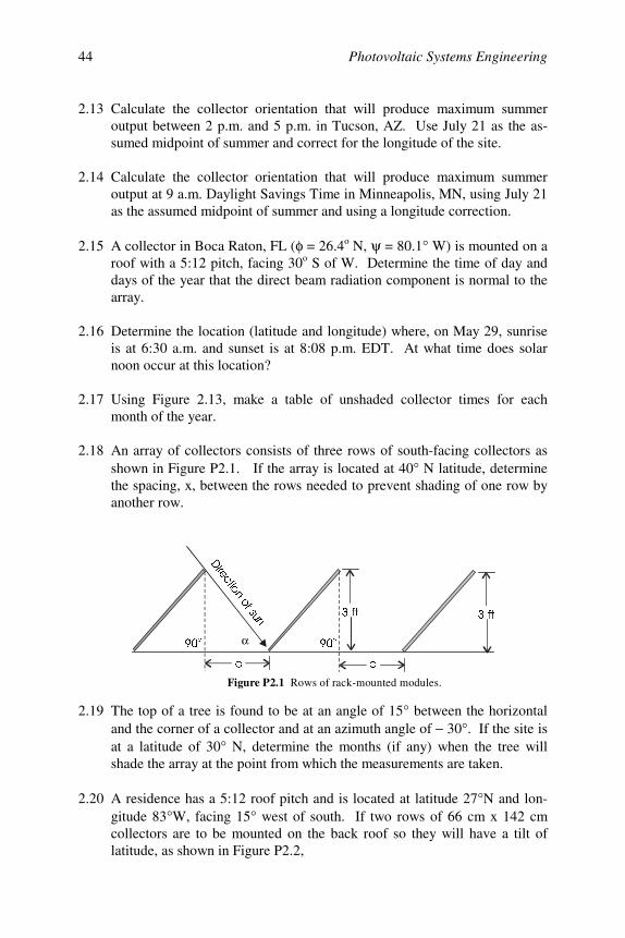
Photovoltaic Systems Engineering44
2.13 Calculate the collector orientation that will produce maximum summeroutput between 2 p.m. and 5 p.m. in Tucson, AZ. Use July 21 as the as-sumed midpoint of summer and correct for the longitude of the site.
2.14 Calculate the collector orientation that will produce maximum summeroutput at 9 a.m. Daylight Savings Time in Minneapolis, MN, using July 21as the assumed midpoint of summer and using a longitude correction.
2.15 A collector in Boca Raton, FL ( φ = 26.4o N, ψ = 80.1° W) is mounted on aroof with a 5:12 pitch, facing 30o S of W. Determine the time of day anddays of the year that the direct beam radiation component is normal to thearray.
2.16 Determine the location (latitude and longitude) where, on May 29, sunriseis at 6:30 a.m. and sunset is at 8:08 p.m. EDT. At what time does solarnoon occur at this location?
2.17 Using Figure 2.13, make a table of unshaded collector times for eachmonth of the year.
2.18 An array of collectors consists of three rows of south-facing collectors asshown in Figure P2.1. If the array is located at 40° N latitude, determinethe spacing, x, between the rows needed to prevent shading of one row byanother row.
2.19 The top of a tree is found to be at an angle of 15° between the horizontaland the corner of a collector and at an azimuth angle of − 30°. If the site isat a latitude of 30° N, determine the months (if any) when the tree willshade the array at the point from which the measurements are taken.
2.20 A residence has a 5:12 roof pitch and is located at latitude 27°N and lon-gitude 83°W, facing 15° west of south. If two rows of 66 cm x 142 cmcollectors are to be mounted on the back roof so they will have a tilt oflatitude, as shown in Figure P2.2,
GG
IW IW
α
'LUHFWLRQRIVX
Q
Figure P2.1 Rows of rack-mounted modules.
R
R
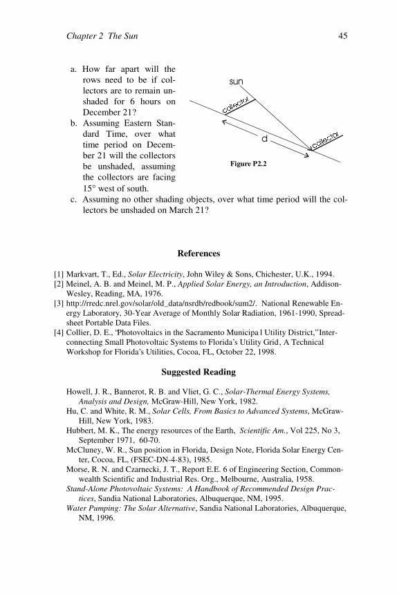
Chapter 2 The Sun 45
a. How far apart will therows need to be if col-lectors are to remain un-shaded for 6 hours onDecember 21?
b. Assuming Eastern Stan-dard Time, over whattime period on Decem-ber 21 will the collectorsbe unshaded, assumingthe collectors are facing15° west of south.
c. Assuming no other shading objects, over what time period will the col-lectors be unshaded on March 21?
References
[1] Markvart, T., Ed., Solar Electricity, John Wiley & Sons, Chichester, U.K., 1994. [2] Meinel, A. B. and Meinel, M. P., Applied Solar Energy, an Introduction, Addison-
Wesley, Reading, MA, 1976. [3] http://rredc.nrel.gov/solar/old_data/nsrdb/redbook/sum2/. National Renewable En-
ergy Laboratory, 30-Year Average of Monthly Solar Radiation, 1961-1990, Spread-sheet Portable Data Files.
[4] Collier, D. E., “Photovoltaics in the Sacramento Municipa l Utility District,” Inter-connecting Small Photovoltaic Systems to Florida’s Utility Grid, A TechnicalWorkshop for Florida’s Utilities, Cocoa, FL, October 22, 1998.
Suggested Reading
Howell, J. R., Bannerot, R. B. and Vliet, G. C., Solar-Thermal Energy Systems,Analysis and Design, McGraw-Hill, New York, 1982.
Hu, C. and White, R. M., Solar Cells, From Basics to Advanced Systems, McGraw-Hill, New York, 1983.
Hubbert, M. K., The energy resources of the Earth, Scientific Am., Vol 225, No 3,September 1971, 60–70.
McCluney, W. R., Sun position in Florida, Design Note, Florida Solar Energy Cen-ter, Cocoa, FL, (FSEC-DN-4-83), 1985.
Morse, R. N. and Czarnecki, J. T., Report E.E. 6 of Engineering Section, Common-wealth Scientific and Industrial Res. Org., Melbourne, Australia, 1958.
Stand-Alone Photovoltaic Systems: A Handbook of Recommended Design Prac-tices, Sandia National Laboratories, Albuquerque, NM, 1995.
Water Pumping: The Solar Alternative, Sandia National Laboratories, Albuquerque,NM, 1996.
FR
OOHFWRU
FROOH
FWRU
Figure P2.2

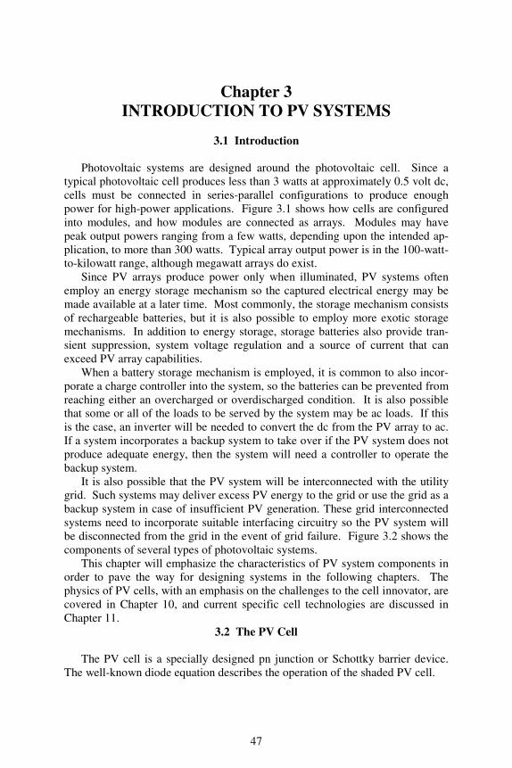
47
Chapter 3INTRODUCTION TO PV SYSTEMS
3.1 Introduction
Photovoltaic systems are designed around the photovoltaic cell. Since atypical photovoltaic cell produces less than 3 watts at approximately 0.5 volt dc,cells must be connected in series-parallel configurations to produce enoughpower for high-power applications. Figure 3.1 shows how cells are configuredinto modules, and how modules are connected as arrays. Modules may havepeak output powers ranging from a few watts, depending upon the intended ap-plication, to more than 300 watts. Typical array output power is in the 100-watt-to-kilowatt range, although megawatt arrays do exist.
Since PV arrays produce power only when illuminated, PV systems oftenemploy an energy storage mechanism so the captured electrical energy may bemade available at a later time. Most commonly, the storage mechanism consistsof rechargeable batteries, but it is also possible to employ more exotic storagemechanisms. In addition to energy storage, storage batteries also provide tran-sient suppression, system voltage regulation and a source of current that canexceed PV array capabilities.
When a battery storage mechanism is employed, it is common to also incor-porate a charge controller into the system, so the batteries can be prevented fromreaching either an overcharged or overdischarged condition. It is also possiblethat some or all of the loads to be served by the system may be ac loads. If thisis the case, an inverter will be needed to convert the dc from the PV array to ac.If a system incorporates a backup system to take over if the PV system does notproduce adequate energy, then the system will need a controller to operate thebackup system.
It is also possible that the PV system will be interconnected with the utilitygrid. Such systems may deliver excess PV energy to the grid or use the grid as abackup system in case of insufficient PV generation. These grid interconnectedsystems need to incorporate suitable interfacing circuitry so the PV system willbe disconnected from the grid in the event of grid failure. Figure 3.2 shows thecomponents of several types of photovoltaic systems.
This chapter will emphasize the characteristics of PV system components inorder to pave the way for designing systems in the following chapters. Thephysics of PV cells, with an emphasis on the challenges to the cell innovator, arecovered in Chapter 10, and current specific cell technologies are discussed inChapter 11.
3.2 The PV Cell
The PV cell is a specially designed pn junction or Schottky barrier device.The well-known diode equation describes the operation of the shaded PV cell.
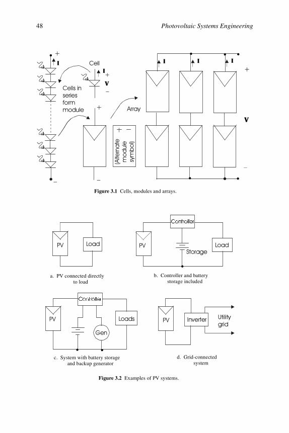
Photovoltaic Systems Engineering48
&RQWUROOHU
a. PV connected directly to load
b. Controller and battery storage included
&RQWUROOHU
c. System with battery storage and backup generator
d. Grid-connected system
Figure 3.2 Examples of PV systems.
Figure 3.1 Cells, modules and arrays.
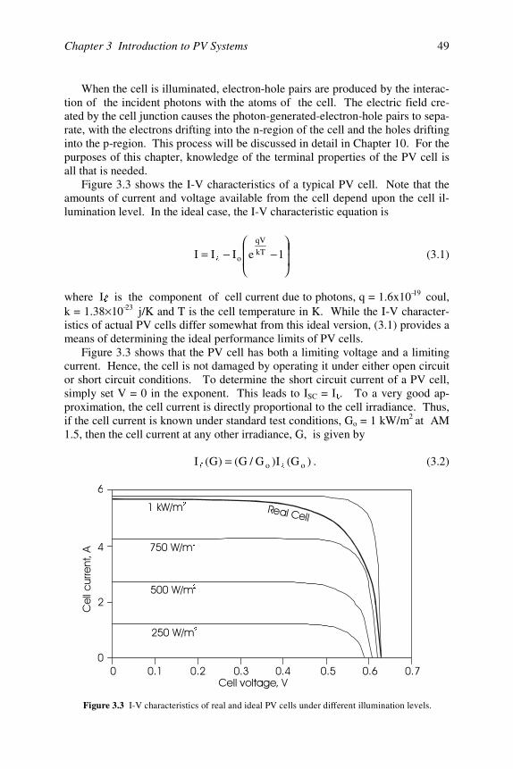
Chapter 3 Introduction to PV Systems 49
When the cell is illuminated, electron-hole pairs are produced by the interac-tion of the incident photons with the atoms of the cell. The electric field cre-ated by the cell junction causes the photon-generated-electron-hole pairs to sepa-rate, with the electrons drifting into the n-region of the cell and the holes driftinginto the p-region. This process will be discussed in detail in Chapter 10. For thepurposes of this chapter, knowledge of the terminal properties of the PV cell isall that is needed.
Figure 3.3 shows the I-V characteristics of a typical PV cell. Note that theamounts of current and voltage available from the cell depend upon the cell il-lumination level. In the ideal case, the I-V characteristic equation is
−−= 1eIII kT
qV
ol (3.1)
where I is the component of cell current due to photons, q = 1.6x10⁻¹⁹ coul,k = 1.38 × 10⁻²³ j/K and T is the cell temperature in K. While the I-V character-istics of actual PV cells differ somewhat from this ideal version, (3.1) provides ameans of determining the ideal performance limits of PV cells.
Figure 3.3 shows that the PV cell has both a limiting voltage and a limitingcurrent. Hence, the cell is not damaged by operating it under either open circuitor short circuit conditions. To determine the short circuit current of a PV cell,simply set V = 0 in the exponent. This leads to ISC = I . To a very good ap-proximation, the cell current is directly proportional to the cell irradiance. Thus,if the cell current is known under standard test conditions, Go = 1 kW/m2 at AM1.5, then the cell current at any other irradiance, G, is given by
)G(I)G/G()G(I oo ll= . (3.2)
!
"# "! "$ "% "& "' "(
) *
*
#+,-
(& ,-
& ,-
!& ,-
.
Figure 3.3 I-V characteristics of real and ideal PV cells under different illumination levels.
%
'

Photovoltaic Systems Engineering50
To determine the open circuit voltage of the cell, the cell current is set tozero and (3.1) is solved for OCV , yielding the result
oo
oOC I
Iln
qkT
I
IIln
qkT
V ll ≅+
= , (3.3)
since normally I >> Io. For example, if the ratio of photocurrent to reversesaturation current is 1010, using a thermal voltage (kT/q) of 26 mV, yields VOC
= 0.6 V. Note that the open circuit voltage is only logarithmically dependent onthe cell illumination, while the short circuit current is directly proportional tocell illumination.
Multiplying the cell current by the cell voltage yields the cell power. In or-der to obtain as much energy as possible from the rather costly PV cell, it is de-sirable to operate the cell to produce maximum power. Referring to Figure 3.4,note that there is one point on the cell I-V characteristic where the cell producesmaximum power. Note also that the voltage at which maximum power occurs isdependent upon the cell illumination level. The maximum power point can beobtained by plotting a set of hyperbolas defined as IV=constant, and noting thepower associated with the hyperbola that is tangent to the cell I-V curve at onlyone point, as opposed to missing the curve or intersecting the curve in twopoints. The maximum power point may also be determined by differentiatingthe cell power equation and setting the result equal to zero. After finding thevoltage for which this condition is satisfied, and checking to verify that thisvoltage represents a maximum, the maximum power point is known. The
!
"! "% "'
) *
*
Figure 3.4 Determination of the maximum power point on a PV cell operating characteristic.
"/
%
'
/
IV = )
PD[
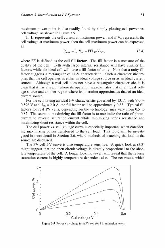
Chapter 3 Introduction to PV Systems 51
maximum power point is also readily found by simply plotting cell power vs.cell voltage, as shown in Figure 3.5.
If Im represents the cell current at maximum power, and if Vm represents thecell voltage at maximum power, then the cell maximum power can be expressedas
,VFFIVIP OCSCmmmax == (3.4)
where FF is defined as the cell fill factor. The fill factor is a measure of thequality of the cell. Cells with large internal resistance will have smaller fillfactors, while the ideal cell will have a fill factor of unity. Note that a unity fillfactor suggests a rectangular cell I-V characteristic. Such a characteristic im-plies that the cell operates as either an ideal voltage source or as an ideal currentsource. Although a real cell does not have a rectangular characteristic, it isclear that it has a region where its operation approximates that of an ideal volt-age source and another region where its operation approximates that of an idealcurrent source.
For the cell having an ideal I-V characteristic governed by (3.1), with VOC =0.596 V and ISC = 2.0 A, the fill factor will be approximately 0.83. Typical fillfactors for real PV cells, depending on the technology, may vary from 0.5 to0.82. The secret to maximizing the fill factor is to maximize the ratio of photo-current to reverse saturation current while minimizing series resistance andmaximizing shunt resistance within the cell.
The cell power vs. cell voltage curve is especially important when consider-ing maximizing power transferred to the cell load. This topic will be investi-gated in more detail in Section 3.6, where methods of matching the load to thesource are discussed.
The PV cell I-V curve is also temperature sensitive. A quick look at (3.3)might suggest that the open circuit voltage is directly proportional to the abso-lute temperature of the cell. A longer look, however, will reveal that the reversesaturation current is highly temperature dependent also. The net result, which
Figure 3.5 Power vs. voltage for a PV cell for 4 illumination levels.
#
!
$
01*,
"! "% "'*
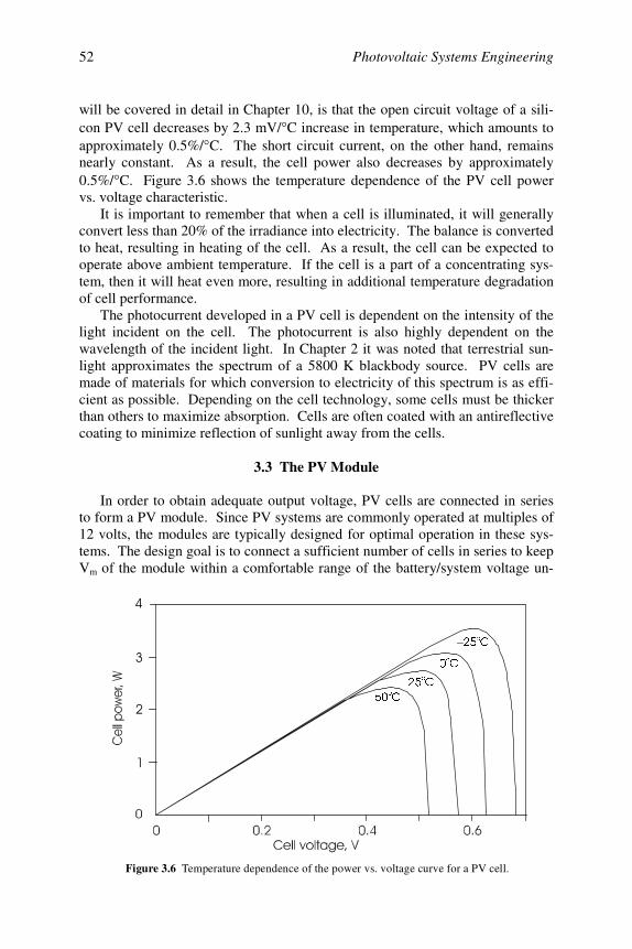
Photovoltaic Systems Engineering52
will be covered in detail in Chapter 10, is that the open circuit voltage of a sili-con PV cell decreases by 2.3 mV/°C increase in temperature, which amounts toapproximately 0.5%/°C. The short circuit current, on the other hand, remainsnearly constant. As a result, the cell power also decreases by approximately0.5%/°C. Figure 3.6 shows the temperature dependence of the PV cell powervs. voltage characteristic.
It is important to remember that when a cell is illuminated, it will generallyconvert less than 20% of the irradiance into electricity. The balance is convertedto heat, resulting in heating of the cell. As a result, the cell can be expected tooperate above ambient temperature. If the cell is a part of a concentrating sys-tem, then it will heat even more, resulting in additional temperature degradationof cell performance.
The photocurrent developed in a PV cell is dependent on the intensity of thelight incident on the cell. The photocurrent is also highly dependent on thewavelength of the incident light. In Chapter 2 it was noted that terrestrial sun-light approximates the spectrum of a 5800 K blackbody source. PV cells aremade of materials for which conversion to electricity of this spectrum is as effi-cient as possible. Depending on the cell technology, some cells must be thickerthan others to maximize absorption. Cells are often coated with an antireflectivecoating to minimize reflection of sunlight away from the cells.
3.3 The PV Module
In order to obtain adequate output voltage, PV cells are connected in seriesto form a PV module. Since PV systems are commonly operated at multiples of12 volts, the modules are typically designed for optimal operation in these sys-tems. The design goal is to connect a sufficient number of cells in series to keepVm of the module within a comfortable range of the battery/system voltage un-
Figure 3.6 Temperature dependence of the power vs. voltage curve for a PV cell.
&R
&R
− &R
&R
#
!
$
%
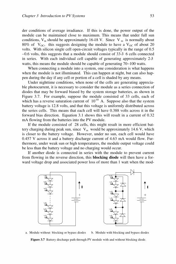
Chapter 3 Introduction to PV Systems 53
der conditions of average irradiance. If this is done, the power output of themodule can be maintained close to maximum. This means that under full sunconditions, Vm should be approximately 16–18 V. Since V m is normally about80% of VOC, this suggests designing the module to have a VOC of about 20volts. With silicon single cell open-circuit voltages typically in the range of 0.5– 0.6 volts, this suggests that a module should consist of 33–3 6 cells connectedin series. With each individual cell capable of generating approximately 2–3watts, this means the module should be capable of generating 70−100 watts.
When connecting a module into a system, one consideration is what happenswhen the module is not illuminated. This can happen at night, but can also hap-pen during the day if any cell or portion of a cell is shaded by any means.
Under nighttime conditions, when none of the cells are generating apprecia-ble photocurrent, it is necessary to consider the module as a series connection ofdiodes that may be forward biased by the system storage batteries, as shown inFigure 3.7. For example, suppose the module consisted of 33 cells, each ofwhich has a reverse saturation current of 10–10 A. Suppose also that the systembattery voltage is 12.8 volts, and that this voltage is uniformly distributed acrossthe series cells. This means that each cell will have 0.388 volts across it in theforward bias direction. Equation 3.1 shows this will result in a current of 0.32mA flowing from the batteries into the PV module.
If the module consisted of 28 cells, this might result in more efficient bat-tery charging during peak sun, since Vm would be approximately 14.6 V, whichis closer to the battery voltage. However, under no sun, each cell would have0.457 V across it and a battery discharge current of 4.63 mA would flow. Fur-thermore, under weak sun or high temperatures, the module output voltage couldbe less than the battery voltage and no charging would occur. If another diode is connected in series with the module to prevent currentfrom flowing in the reverse direction, this blocking diode will then have a for-ward voltage drop and associated power loss of more than 1 watt when the mod-
a. Module without blocking or bypass diodes b. Module with blocking and bypass diodes
Figure 3.7 Battery discharge path through PV module with and without blocking diode.
Photovoltaic Systems Engineering54
ule is providing photocurrent. If the module is only providing 50 watts, thisloss represents 2–3% of the total module output power. The bot tom line is thatit is more efficient to simply have more cells in the series connection. In fact,blocking diodes are rarely used in PV systems. The exact number of cells willdepend on the performance characteristics of the individual cell. Manufacturersof modules specify the open circuit voltage and short circuit current of the mod-ules along with the module maximum power rating under full sun test condi-tions. These parameters are shown in Figure 3.4 for individual cells.
Another important observation relating to the series connection of PV cellsrelates to shading of individual cells. If any one of the cells in a module shouldbe shaded, the performance of that cell will be degraded. Since the cells are inseries, this means that the cell may become forward biased if other unshadedmodules are connected in parallel, resulting in heating of the cell. This phe-nomenon can cause premature cell failure. To protect the system against suchfailure, modules are generally protected with bypass diodes, as shown in Figure3.7. If PV current cannot flow through one or more the PV cells in the module,it will flow through the bypass diode instead. When cells are mounted into modules, they are often covered withantireflective coating, then with a special laminate to prevent degradation of thecell contacts. The module housing is generally metal, which provides physicalstrength to the module. When the PV cells are mounted in the module, they canbe characterized as having a nominal operating cell temperature (NOCT).The NOCT is the temperature the cells will reach when operated at open circuitin an ambient temperature of 20oC at AM 1.5 irradiance conditions, G = 0.8kW/m2 and a wind speed less than 1 m/s. For variations in ambient temperatureand irradiance the cell temperature (in oC) can be estimated quite accurately withthe linear approximation that
G8.0
20NOCTTT AC
−+= . (3.5)
The combined effects of irradiance and ambient temperature on cell perform-ance merit careful consideration. Since the open circuit voltage of a silicon celldecreases by 2.3 mV/oC, the open circuit voltage of a module will decrease by2.3n mV/oC, where n is the number of series cells in the module. Hence, for example, if a 36-cell module has a NOCT of 40oC with VOC =19.40 V, when G = 0.8 kW/m2, then the cell temperature will rise to 55oCwhen the ambient temperature rises to 30oC and G increases to 1 kW/m2. This15oC increase in cell temperature will result in a decrease of the open circuitvoltage to 18.16 V, a 6% decrease. Furthermore, excessive temperature eleva-tion may cause the cell to fail prematurely. Finally, a word about module efficiency. It is important to note that the effi-ciency of a module will be determined by its weakest link. Since the cells areseries connected, it is important that cells in the module be matched as closely aspossible. If this is not the case, while some cells are operating at peak effi-ciency, others may not be optimized. As a result, the power output from the
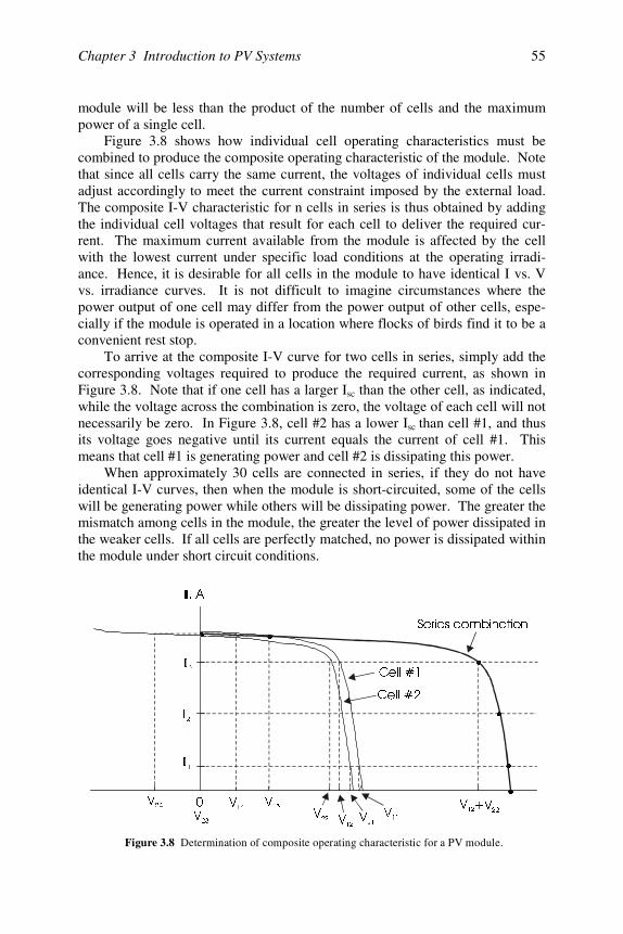
Chapter 3 Introduction to PV Systems 55
module will be less than the product of the number of cells and the maximumpower of a single cell.
Figure 3.8 shows how individual cell operating characteristics must becombined to produce the composite operating characteristic of the module. Notethat since all cells carry the same current, the voltages of individual cells mustadjust accordingly to meet the current constraint imposed by the external load.The composite I-V characteristic for n cells in series is thus obtained by addingthe individual cell voltages that result for each cell to deliver the required cur-rent. The maximum current available from the module is affected by the cellwith the lowest current under specific load conditions at the operating irradi-ance. Hence, it is desirable for all cells in the module to have identical I vs. Vvs. irradiance curves. It is not difficult to imagine circumstances where thepower output of one cell may differ from the power output of other cells, espe-cially if the module is operated in a location where flocks of birds find it to be aconvenient rest stop.
To arrive at the composite I-V curve for two cells in series, simply add thecorresponding voltages required to produce the required current, as shown inFigure 3.8. Note that if one cell has a larger Isc than the other cell, as indicated,while the voltage across the combination is zero, the voltage of each cell will notnecessarily be zero. In Figure 3.8, cell #2 has a lower Isc than cell #1, and thusits voltage goes negative until its current equals the current of cell #1. Thismeans that cell #1 is generating power and cell #2 is dissipating this power.
When approximately 30 cells are connected in series, if they do not haveidentical I-V curves, then when the module is short-circuited, some of the cellswill be generating power while others will be dissipating power. The greater themismatch among cells in the module, the greater the level of power dissipated inthe weaker cells. If all cells are perfectly matched, no power is dissipated withinthe module under short circuit conditions.
q
q q
q
q
q
,$
&HOO
&HOO
9
99
9
9
9
9
9
9
9
6HULHVFRPELQDWLRQ
,
,
,
Figure 3.8 Determination of composite operating characteristic for a PV module.
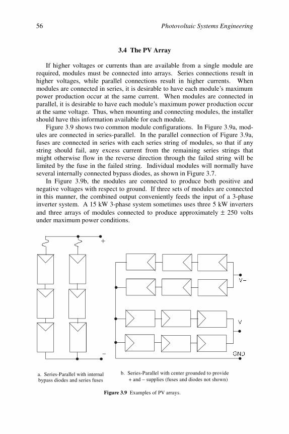
Photovoltaic Systems Engineering56
3.4 The PV Array
If higher voltages or currents than are available from a single module arerequired, modules must be connected into arrays. Series connections result inhigher voltages, while parallel connections result in higher currents. Whenmodules are connected in series, it is desirable to have each module’s maximumpower production occur at the same current. When modules are connected inparallel, it is desirable to have each module’s maximum power production occurat the same voltage. Thus, when mounting and connecting modules, the installershould have this information available for each module.
Figure 3.9 shows two common module configurations. In Figure 3.9a, mod-ules are connected in series-parallel. In the parallel connection of Figure 3.9a,fuses are connected in series with each series string of modules, so that if anystring should fail, any excess current from the remaining series strings thatmight otherwise flow in the reverse direction through the failed string will belimited by the fuse in the failed string. Individual modules will normally haveseveral internally connected bypass diodes, as shown in Figure 3.7.
In Figure 3.9b, the modules are connected to produce both positive andnegative voltages with respect to ground. If three sets of modules are connectedin this manner, the combined output conveniently feeds the input of a 3-phaseinverter system. A 15 kW 3-phase system sometimes uses three 5 kW invertersand three arrays of modules connected to produce approximately ± 250 voltsunder maximum power conditions.
a. Series-Parallel with internalbypass diodes and series fuses
9
9B
*1'
b. Series-Parallel with center grounded to provide + and supplies (fuses and diodes not shown)−
Figure 3.9 Examples of PV arrays.
Chapter 3 Introduction to PV Systems 57
3.5 Energy Storage
3.5.1 Introduction
Most electrical engineers have some familiarity with batteries, especially theones used in flashlights, toys, laptop computers, watches, calculators, videocameras, automobiles and golf carts. The extent of familiarity normally extendsto the decision as to whether to purchase C-Zn batteries or whether to buy themore expensive, but longer lasting, alkaline cells. Remembering to get the cor-rect size, whether a 9-volt or a 1.5-volt AA battery is another of life’s energystorage dilemmas. In this section, considerations in battery selection for PVsystems are presented. Alternatives to battery energy storage are also presented,so the PV design engineer will be able to make educated choices, based onsound economic and engineering principles, as to which type of energy storageto incorporate into a specific PV system design.
Many different types of rechargeable batteries suitable for PV applicationsare currently available. Although several rather exotic technologies are nowavailable, the lead-acid battery is still the most common for relatively economi-cal storage of relatively large quantities of electrical energy, and will probablyremain so for at least the next few years. However, unless improvements inenergy density, cost and lifetime are made with lead-acid technology, otherpromising technologies may surpass lead-acid technology. For example, Ni-Cdbatteries are in common use in applications that require sealed batteries capableof operating in any position, and still require high energy density. But they aremore expensive per joule stored than lead-acid units. Nickel metal hydride andseveral lithium technologies may also one day provide cost effective storage.
But, then, batteries are not the only way to store energy. It is also possible tostore energy by producing hydrogen, by pumping water uphill, by spinning aflywheel or by charging a large chemical capacitor. This section explores theapplications, advantages and disadvantages of some of the storage methods cur-rently in use as well as some of the new ideas that have been proposed.
3.5.2 The Lead-Acid Storage Battery
Chemistry of the Lead-Acid CellFigure 3.10 shows the basics of lead-acid cell operation. In simple terms, the
battery consists of a lead cathode and a lead oxide (PbO2) anode immersed in asulfuric acid solution. The discharging reaction at the anode consists of the ex-change of oxygen ions from the anode with sulfate ions of the electrolyte. Atthe cathode, the discharge involves sulfate ions from the electrolyte combiningwith lead ions to form lead sulfate. Removal of sulfate ions from the solutionreduces the acidity of the electrolyte. To maintain charge neutrality, two elec-trons must enter the anode terminal and two electrons must leave the cathodeterminal via the external circuit for each two sulfate ions that leave the electro-lyte. This corresponds to a positive current leaving the anode terminal, which is
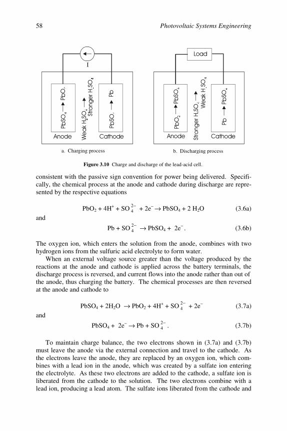
Photovoltaic Systems Engineering58
consistent with the passive sign convention for power being delivered. Specifi-cally, the chemical process at the anode and cathode during discharge are repre-sented by the respective equations
PbO2 + 4H+ + SO 42− + 2e− → PbSO4 + 2 H2O (3.6a)
and
Pb + SO 42− → PbSO4 + 2e− . (3.6b)
The oxygen ion, which enters the solution from the anode, combines with twohydrogen ions from the sulfuric acid electrolyte to form water.
When an external voltage source greater than the voltage produced by thereactions at the anode and cathode is applied across the battery terminals, thedischarge process is reversed, and current flows into the anode rather than out ofthe anode, thus charging the battery. The chemical processes are then reversedat the anode and cathode to
PbSO4 + 2H2O → PbO2 + 4H+ + SO 42− + 2e− (3.7a)
and
PbSO4 + 2e− → Pb + SO 42− . (3.7b)
To maintain charge balance, the two electrons shown in (3.7a) and (3.7b)must leave the anode via the external connection and travel to the cathode. Asthe electrons leave the anode, they are replaced by an oxygen ion, which com-bines with a lead ion in the anode, which was created by a sulfate ion enteringthe electrolyte. As these two electrons are added to the cathode, a sulfate ion isliberated from the cathode to the solution. The two electrons combine with alead ion, producing a lead atom. The sulfate ions liberated from the cathode and
I
a. Charging process b. Discharging process
Figure 3.10 Charge and discharge of the lead-acid cell.
Chapter 3 Introduction to PV Systems 59
the anode to the solution increase the concentration of sulfuric acid in the elec-trolyte solution by balancing with hydrogen ions in the solution, while the oxy-gen ion left behind by the dissociated water molecule is left alone in solution.The positive potential difference between anode and cathode causes the nega-tively charged oxygen ion to migrate to the anode, where it becomes a part ofthe anode reaction, ultimately being converted to lead oxide at the anode, aspreviously indicated. When the battery discharges, ultimately the surfaces of both electrodes areconverted to lead sulfate. If excessive lead sulfate is allowed to build up on theelectrodes, the effective surface area of the electrodes is reduced and cell per-formance may be affected. It is thus important to avoid fully discharging a lead-acid battery. During the charging process, some of the hydrogen ions combinewith free electrons and are converted into gaseous hydrogen. At a certain pointduring charging, when the cathode is fully converted back to lead, there is nomore sulfate at the cathode to maintain continuity in the charging current. Atthis point, if charging is continued, the electrons entering the cathode can nolonger release sulfate ions, so the electrons continue into the electrolyte, com-bine with hydrogen ions, and produce hydrogen gas. This phenomenon is calledgassing, and it is generally not desirable to charge a battery beyond this point,since the hydrogen gas can present a safety hazard. Occasional charging of abattery to the gassing stage so the gas bubbles up through the electrolyte can beuseful, however, since the bubbling action tends to perform a cleaning action onthe electrodes and a mixing action on the electrolyte. The potential difference between electrodes in the lead-acid system is ap-proximately 2.12 volts when the cell is fully charged. As cells are connected inseries, multiples of 2.12 volts can be achieved. Most commonly, either three orsix cells are connected in series, producing nominal voltages of 6 or 12 volts.
Properties of the Lead-Acid Storage BatteryIdeally, the charging and discharging processes of the lead-acid system
should be reversible. In reality, however, they are not. The temperature of op-eration, the rate of discharge and the rate of charge all affect the performance ofthe battery. Since the electrical path of the battery presents ohmic resistance,some of the electrical energy intended for charging, i.e., storage, is converted toheat. When hydrogen is lost, it also represents an energy loss. Typically, thecharging process is about 95% efficient. The discharge process also results insome losses due to internal resistance of the battery, so only about 95% of thestored energy can be recovered. The overall efficiency of charging and dis-charging a lead-acid battery is thus about 90%.
Since battery losses to internal resistance are proportional to the square ofthe current, this means that high current charging or high current dischargingwill tend to result in higher internal losses and less overall performance effi-ciency. This effect is offset somewhat by the increase in temperature of thebattery during charging or discharging at high rates due to the higher I2R losses.It turns out that a warmer battery can hold more charge. It also turns out that if a
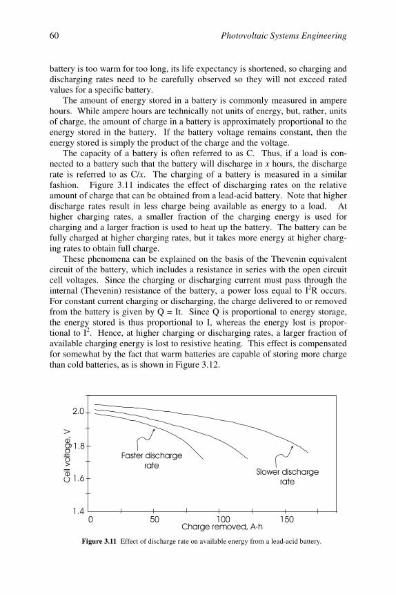
Photovoltaic Systems Engineering60
battery is too warm for too long, its life expectancy is shortened, so charging anddischarging rates need to be carefully observed so they will not exceed ratedvalues for a specific battery.
The amount of energy stored in a battery is commonly measured in amperehours. While ampere hours are technically not units of energy, but, rather, unitsof charge, the amount of charge in a battery is approximately proportional to theenergy stored in the battery. If the battery voltage remains constant, then theenergy stored is simply the product of the charge and the voltage.
The capacity of a battery is often referred to as C. Thus, if a load is con-nected to a battery such that the battery will discharge in x hours, the dischargerate is referred to as C/x. The charging of a battery is measured in a similarfashion. Figure 3.11 indicates the effect of discharging rates on the relativeamount of charge that can be obtained from a lead-acid battery. Note that higherdischarge rates result in less charge being available as energy to a load. Athigher charging rates, a smaller fraction of the charging energy is used forcharging and a larger fraction is used to heat up the battery. The battery can befully charged at higher charging rates, but it takes more energy at higher charg-ing rates to obtain full charge.
These phenomena can be explained on the basis of the Thevenin equivalentcircuit of the battery, which includes a resistance in series with the open circuitcell voltages. Since the charging or discharging current must pass through theinternal (Thevenin) resistance of the battery, a power loss equal to I2R occurs.For constant current charging or discharging, the charge delivered to or removedfrom the battery is given by Q = It. Since Q is proportional to energy storage,the energy stored is thus proportional to I, whereas the energy lost is propor-tional to I2. Hence, at higher charging or discharging rates, a larger fraction ofavailable charging energy is lost to resistive heating. This effect is compensatedfor somewhat by the fact that warm batteries are capable of storing more chargethan cold batteries, as is shown in Figure 3.12.
!
"
#
$ $
%&'&(
)'&(
Figure 3.11 Effect of discharge rate on available energy from a lead-acid battery.
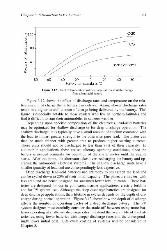
Chapter 3 Introduction to PV Systems 61
Figure 3.12 shows the effect of discharge rates and temperature on the rela-tive amount of charge that a battery can deliver. Again, slower discharge ratesresult in a higher overall amount of charge being delivered by the battery. Thisfigure is especially notable to those readers who live in northern latitudes andfind it difficult to start their automobiles in subzero weather.
Depending upon specific composition of the electrodes, lead-acid batteriesmay be optimized for shallow discharge or for deep discharge operation. Theshallow discharge units typically have a small amount of calcium combined withthe lead to impart greater strength to the otherwise pure lead. The plates canthen be made thinner with greater area to produce higher starting currents.These units should not be discharged to less than 75% of their capacity. Inautomobile applications, these are satisfactory operating conditions, since thebattery is needed primarily for operation of the starter motor until the enginestarts. After this point, the alternator takes over, recharging the battery and op-erating the automobile electrical systems. The shallow discharge units have asmaller quantity of lead and are correspondingly less expensive.
Deep discharge lead-acid batteries use antimony to strengthen the lead andcan be cycled down to 20% of their initial capacity. The plates are thicker, withless area and are hence designed for sustained lower level currents. These bat-teries are designed for use in golf carts, marine applications, electric forkliftsand for PV system use. Although the deep discharge batteries are designed fordeep discharge applications, their lifetime in cycles depends on the depth of dis-charge during normal operation. Figure 3.13 shows how the depth of dischargeaffects the number of operating cycles of a deep discharge battery. The PVsystem designer must carefully consider the trade-off between using more bat-teries operating at shallower discharge rates to extend the overall life of the bat-teries vs. using fewer batteries with deeper discharge rates and the correspond-ingly lower initial cost. Life cycle costing of systems will be considered inChapter 5.
%DWWHU\WHPSHUDWXUH &
R
3HUFHQWRIUDWHGFDSDFLW\
&
&
&
'LVFKDUJHUDWHV
Figure 3.12 Effect of temperature and discharge rate on available energyfrom a lead-acid battery.
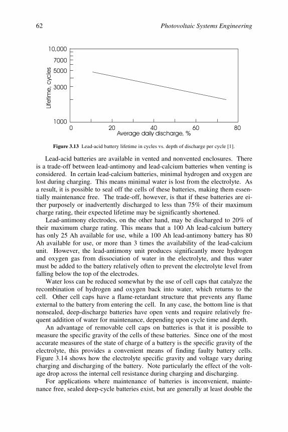
Photovoltaic Systems Engineering62
Lead-acid batteries are available in vented and nonvented enclosures. Thereis a trade-off between lead-antimony and lead-calcium batteries when venting isconsidered. In certain lead-calcium batteries, minimal hydrogen and oxygen arelost during charging. This means minimal water is lost from the electrolyte. Asa result, it is possible to seal off the cells of these batteries, making them essen-tially maintenance free. The trade-off, however, is that if these batteries are ei-ther purposely or inadvertently discharged to less than 75% of their maximumcharge rating, their expected lifetime may be significantly shortened.
Lead-antimony electrodes, on the other hand, may be discharged to 20% oftheir maximum charge rating. This means that a 100 Ah lead-calcium batteryhas only 25 Ah available for use, while a 100 Ah lead-antimony battery has 80Ah available for use, or more than 3 times the availability of the lead-calciumunit. However, the lead-antimony unit produces significantly more hydrogenand oxygen gas from dissociation of water in the electrolyte, and thus watermust be added to the battery relatively often to prevent the electrolyte level fromfalling below the top of the electrodes.
Water loss can be reduced somewhat by the use of cell caps that catalyze therecombination of hydrogen and oxygen back into water, which returns to thecell. Other cell caps have a flame-retardant structure that prevents any flameexternal to the battery from entering the cell. In any case, the bottom line is thatnonsealed, deep-discharge batteries have open vents and require relatively fre-quent addition of water for maintenance, depending upon cycle time and depth.
An advantage of removable cell caps on batteries is that it is possible tomeasure the specific gravity of the cells of these batteries. Since one of the mostaccurate measures of the state of charge of a battery is the specific gravity of theelectrolyte, this provides a convenient means of finding faulty battery cells.Figure 3.14 shows how the electrolyte specific gravity and voltage vary duringcharging and discharging of the battery. Note particularly the effect of the volt-age drop across the internal cell resistance during charging and discharging.
For applications where maintenance of batteries is inconvenient, mainte-nance free, sealed deep-cycle batteries exist, but are generally at least double the
# " !'*'&(+
,
$
-
'.'(*(&
Figure 3.13 Lead-acid battery lifetime in cycles vs. depth of discharge per cycle [1].
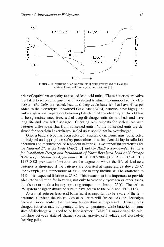
Chapter 3 Introduction to PV Systems 63
price of equivalent capacity nonsealed lead-acid units. These batteries are valveregulated to recombine gases, with additional treatment to immobilize the elec-trolyte. Gel Cells are sealed, lead-acid deep-cycle batteries that have silica geladded to the electrolyte. Absorbed Glass Mat (AGM) batteries have highly ab-sorbent glass mat separators between plates to bind the electrolyte. In additionto being maintenance free, sealed deep-discharge units do not leak and havelong life and low self-discharge. Charging requirements for sealed lead acidbatteries differ somewhat from nonsealed units. While nonsealed units are de-signed for occasional overcharge, sealed units should not be overcharged.
Once a battery type has been selected, a suitable enclosure must be selectedor designed and appropriate safety precautions must be taken during installation,operation and maintenance of lead-acid batteries. Two important references arethe National Electrical Code (NEC) [2] and the IEEE Recommended Practicefor Installation Design and Installation of Valve-Regulated Lead-Acid StorageBatteries for Stationary Applications (IEEE 1187-2002 [3]). Annex C of IEEE1187-2002 provides information on the degree to which the life of lead-acidbatteries is shortened if the batteries are operated at temperatures above 25°C.For example, at a temperature of 35°C, the battery lifetime will be shortened to44% of its expected lifetime at 25°C. This means that it is important to provideadequate ventilation for batteries, not only to vent any hydrogen or other gases,but also to maintain a battery operating temperature close to 25°C. The seriousPV system designer should be sure to have access to the NEC and IEEE 1187.
As a final note on lead-acid batteries, it is important to be aware of the tem-peratures at which the electrolytes of batteries will freeze. As the electrolytebecomes more acidic, the freezing temperature is depressed. Hence, fullycharged batteries may be operated at low temperatures, while batteries in somestate of discharge will need to be kept warmer. Table 3.1 summarizes the rela-tionships between state of charge, specific gravity, cell voltage and electrolytefreezing point.
7LPH
'LVFKDUJH &KDUJH
&HOO
YROWDJH6SHFLILF
JUDYLW\&HOOYROWDJH9
&HOOVSHFLILFJUDYLW\
Figure 3.14 Variation of cell electrolyte specific gravity and cell voltageduring charge and discharge at constant rate [1].
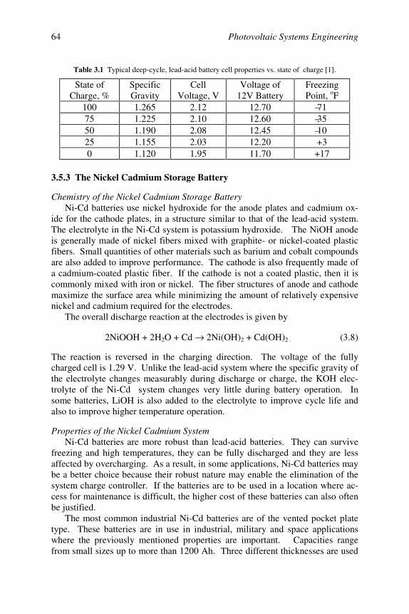
Photovoltaic Systems Engineering64
Table 3.1 Typical deep-cycle, lead-acid battery cell properties vs. state of charge [1].
State ofCharge, %
SpecificGravity
CellVoltage, V
Voltage of12V Battery
FreezingPoint, oF
100 1.265 2.12 12.70 –7175 1.225 2.10 12.60 –3550 1.190 2.08 12.45 –1025 1.155 2.03 12.20 +30 1.120 1.95 11.70 +17
3.5.3 The Nickel Cadmium Storage Battery
Chemistry of the Nickel Cadmium Storage BatteryNi-Cd batteries use nickel hydroxide for the anode plates and cadmium ox-
ide for the cathode plates, in a structure similar to that of the lead-acid system.The electrolyte in the Ni-Cd system is potassium hydroxide. The NiOH anodeis generally made of nickel fibers mixed with graphite- or nickel-coated plasticfibers. Small quantities of other materials such as barium and cobalt compoundsare also added to improve performance. The cathode is also frequently made ofa cadmium-coated plastic fiber. If the cathode is not a coated plastic, then it iscommonly mixed with iron or nickel. The fiber structures of anode and cathodemaximize the surface area while minimizing the amount of relatively expensivenickel and cadmium required for the electrodes.
The overall discharge reaction at the electrodes is given by
2NiOOH + 2H2O + Cd → 2Ni(OH)2 + Cd(OH)2 . (3.8)
The reaction is reversed in the charging direction. The voltage of the fullycharged cell is 1.29 V. Unlike the lead-acid system where the specific gravity ofthe electrolyte changes measurably during discharge or charge, the KOH elec-trolyte of the Ni-Cd system changes very little during battery operation. Insome batteries, LiOH is also added to the electrolyte to improve cycle life andalso to improve higher temperature operation.
Properties of the Nickel Cadmium SystemNi-Cd batteries are more robust than lead-acid batteries. They can survive
freezing and high temperatures, they can be fully discharged and they are lessaffected by overcharging. As a result, in some applications, Ni-Cd batteries maybe a better choice because their robust nature may enable the elimination of thesystem charge controller. If the batteries are to be used in a location where ac-cess for maintenance is difficult, the higher cost of these batteries can also oftenbe justified.
The most common industrial Ni-Cd batteries are of the vented pocket platetype. These batteries are in use in industrial, military and space applicationswhere the previously mentioned properties are important. Capacities rangefrom small sizes up to more than 1200 Ah. Three different thicknesses are used
Chapter 3 Introduction to PV Systems 65
for electrodes, depending on whether the battery is designed for high, medium orlow discharge rates.
Energy densities range from 20 Wh/kg for the pocket plate batteries to morethan 50 Wh/kg when cells are made of the plastic-bonded plates.
Unlike the lead-acid system, which loses capacity under conditions of heavydischarge, the Ni-Cd system can be discharged at rates up to C over a wide tem-perature range, while still providing more than 90% of its capacity to the load.This is partially attributable to the very low internal resistance of the cells,which, depending on cell area, can be less than a milliohm.
If Ni-Cd batteries are charged and then left unused, they will lose charge atthe rate of approximately 2% per day for the first few days, but then stabilize toa relatively low loss rate. Over a 6-month period, the total loss is typically about20%, depending on whether the battery is a high, medium or low discharge ratebattery. The higher the discharge rating of the battery, the greater the loss ofcharge over time.
Loss of charge is also temperature dependent. The loss rate is greater athigher temperatures, but at a temperature of –20 oC, there is almost no loss at all.
The lifetime of a Ni-Cd battery depends on how it is used, but is less de-pendent on depth of discharge than that of lead-acid batteries. A lifetime of atleast 2000 cycles can be expected for a battery when it is not used extensively atelevated temperatures. As a result, under certain applications and operatingconditions, a battery may last as long as 25 years, while under more frequentcycling, the lifetime may be reduced to 8 years. It is not unreasonable to expecta Ni-Cd battery to last twice as long as its lead-acid counterpart.
Ni-Cd batteries may be charged at either constant current, constant voltageor somewhere in between. This makes them especially useful in PV applica-tions, since a PV array tends to act as a constant current source, depending onthe cloud cover at the moment. If Ni-Cd batteries are overcharged, gassing willoccur and the water in the electrolyte will decompose, creating a need for moremaintenance. Normally, charging from full discharge to full charge should beaccomplished in 5 to 7 hours, with a charging voltage between 1.50 and 1.65volts per cell. The ampere-hour charging efficiency of the most efficient Ni-Cdbatteries approaches 85%.
Those proud owners of camcorders, computers or electric toothbrushes withNi-Cd batteries are probably familiar with the memory effect. If the battery isnot fully discharged prior to recharge, the battery will tend to discharge only tothe point where it was most recently discharged, and then lose cell voltage. Thisis manifested in the 1-hour battery lasting only for 15 minutes before the chargelight comes on and the camcorder shuts down. Fortunately, the memory effectis predominant in sealed batteries and is not a problem in a battery with eitherpocket, fiber or plastic-bonded plate cells.
Sealed Ni-Cd batteries are also available, but their cost is higher. Their ad-vantages over the vented units include maintenance-free operation, high dis-charge rates and high charge rates, along with wide temperature range. How-ever, presently they are only available in sizes under 35 Ah.

Photovoltaic Systems Engineering66
Disadvantages of Ni-Cd batteries include difficulty in determining the stateof charge of the batteries and the toxicity of the cadmium, which creates an en-vironmental concern during production and disposal.
3.5.4 Other Battery Systems [4]
A number of other battery systems are currently in use, and others seem toshow promise for future use. The nickel-zinc battery is a combination of theNi-Cd system and the Cu-Zn system, which provides some attractive features,including long life and a capacity advantage. The specific energy of the Ni-Znsystem is double the specific energy of the Ni-Cd system. The overall dischargechemical reaction is given by
2NiOOH + Zn + 2H2O → 2Ni(OH)2 + Zn(OH)2 . (3.9)
If the battery is allowed to overcharge, it dissociates the water in the KOH elec-trolyte, resulting in gassing and the release of hydrogen and oxygen. Hence,charging must be controlled to avoid overcharging. Fully charged cell voltage isapproximately 1.73 V.
Ni-Zn battery systems can be made in sizes in excess of 200 Ah. At normaloperating temperatures ( ≅ 20oC) and reasonable discharge rates ( ≅ C/3) the cellvoltage remains quite stable at about 1.6 volts over most of the discharge range.
Another technology that is becoming very popular, particularly in smallerapplications such as camcorders and laptop computers, is the nickel-metal hy-dride (NIMH) battery. This battery replaces the cadmium cathode with an envi-ronmentally benign metal hydride cathode, allowing for higher energy density atthe cathode and a correspondingly longer lifetime or higher capacity, dependingon the design goal. The anode is the same as in the Ni-Cd cell and KOH is usedas the electrolyte. The overall discharge reaction is
MH + NiOOH → M + Ni(OH)2 . (3.10)
The NIMH cell requires clever use of an oxygen recombination system toprevent loss of oxygen during the charging cycle. Electrodes are also carefullysized to ensure that the useful capacity of the battery is determined by the anodeelectrode to ensure that the cathode will moderate any overcharge or overdis-charge condition.
A number of additional battery types are currently under investigation forPV and similar uses, such as electric vehicles. A partial listing of these batteriesincludes zinc/silver oxide, metal/air, iron/air, zinc/air, aluminum/air, lithium/air,zinc/bromine, lithium-aluminum/iron sulfide, lithium-aluminum/iron disulfide,sodium/sulfur, sodium/metal chloride and several variations of lithium ambienttemperature batteries.
The lithium technologies appear quite attractive due to energy densities up to150 Wh/kg, cell voltages up to 4 V and long charge retention and shelf life.Other problems must be overcome, however, before use of these batteries be-comes widespread. For example, they have low cycle life, relatively poor high-
Chapter 3 Introduction to PV Systems 67
rate performance, relatively poor low-temperature performance, capacity fadingand potential safety problems. It should be remembered that metallic lithium ishighly reactive and presents a danger if it contacts water or humans.
The young engineer can expect to see progress in these new technologiesduring his/her path toward becoming an older engineer. In addition to batterystorage, which is presently the most common method of energy storage for PVsystems, a number of other energy storage methods are either in use or havebeen proposed. Many of these methods will also require a significant researcheffort to bring them into cost-effective, production scale use.
3.5.5 Hydrogen Storage [5]
Aside from using batteries to store energy produced by PV systems, it is alsopossible to use hydrogen as a storage medium. The advantage of using hydro-gen for energy storage is when it is desired to recover the stored energy, the hy-drogen is reacted with oxygen to form water, which is an exothermic reactionthat does not have any carbon byproducts. If the hydrogen is burned in air toproduce steam to turn a turbine to generate electricity, water is still produced asthe byproduct, with a relatively minimal amount of nitrogen oxides. Of course,the hydrogen does not need to be used to produce electricity. It can also be usedas an engine fuel to power a vehicle, such as an automobile, bus or space shuttle.Indirectly, the result is a solar-powered vehicle that stores energy in hydrogenrather than in batteries. The engineering community has not yet developed abattery-powered, space shuttle booster engine.
Perhaps the most important advantage of hydrogen storage is the energydensity of hydrogen. One of the highest energy densities in conventional fuels isthat of gasoline, which contains approximately 1,047,000 Btu/ft3. To store thesame amount of energy in high capacity storage batteries would require ap-proximately 120 batteries having approximately 2000 Btu/ft3 storage capacity.The storage capacity of liquid hydrogen is close to 240,000 Btu/ft3, and gaseoushydrogen can store approximately 47,000 Btu/ft3. Since water cannot be de-composed into gasoline, however, and since gasoline burning produces CO2,among other undesirable combustion products, clean burning hydrogen is amore attractive alternative for combustion. Aside from liquid and gaseous hy-drogen storage, other means of obtaining relatively high energy density, includ-ing various hydrides, are also available.
Hydrogen is normally obtained by the electrolysis of water. The output of aPV system is conveniently dc at a level consistent with that needed for relativelyefficient electrolysis. Production of hydrogen by electrolysis may seem to besimply a matter of passing a current through water to produce hydrogen andoxygen, just as many readers have already done in chemistry lab. The challengeis to produce hydrogen efficiently with a system whose power output varies sig-nificantly whenever a cloud passes over the PV array.
First of all, pure water is not a good conductor. Thus, to increase efficiency,something needs to be dissolved in the water to increase the conductivity. Sev-
Photovoltaic Systems Engineering68
eral electrolytes are in common use, and others have been proposed that seem toshow promise for higher efficiency conversion.
Once the hydrogen is produced, it can be used on site or it can be transportedto other locations. Hydrogen proponents have suggested that hydrogen be pro-duced in tropical latitudes having greater annual insolation and shipped to re-gions having less sun. Thus, after the production of hydrogen, storage andtransport of the gas also present engineering challenges.
Recent interest in fuel cells for use in automotive applications has once againpiqued interest in the efficient and convenient production of hydrogen. Thesame technology that may emerge for automotive fuel cell applications mayvery well spin off into PV energy storage applications as well.
3.5.6 The Fuel Cell
Fuel cells provide a convenient means of reacting hydrogen and oxygen di-rectly to produce electricity and water. They utilize essentially the inverse of theelectrolysis process. The first fuel cell was built in 1839 by Sir William Grove[6]. The high cost of fuel cells, however, had kept them out of practical useuntil NASA decided to use them on space flights to provide power and water.Table 3.2 summarizes the five types of fuel cells currently in use.
Fuel cells are being constructed in a wide range of power output capabilities.The smaller cells are sized to power video cameras and laptop computers. On alarger scale, The Southern California Gas Company had ten 200-kW plants online in 1993 and experimental units in the megawatt range are now in operation[6]. The fuel cell reaction is exothermic, so if cleverly applied, the cells cansupply both heat and electricity to a building. By capturing the heat, the overallsystem efficiency is increased, provided that the heat can be put to good use,such as for district heating or other space or water heating application.
The alkaline cell (AFC) contains a 30% solution of KOH as the electrolyte.The proton exchange (or polymer electrolyte) membrane cell (PEMFC) incorpo-rates a semipermeable membrane that will pass hydrogen ions, resulting in aproton exchange. The phosphoric acid cell (PAFC) is based on a 103% phos-phoric acid solution. The molten carbonate cell (MCFC) is based on a eutecticmixture of molten lithium carbonate and potassium carbonate. The solid oxidecell (SOFC) is based on a stabilized zirconium oxide electrolyte.
The low temperature cells are approximately twice as efficient as conven-tional heat engines in the conversion of energy stored in hydrogen to electricity.This makes fuel cells a very attractive possibility for energy storage and conver-sion to electricity in an electric vehicle, since electric motors can be operated atvery high efficiency, especially with modern solid-state controllers. The pres-ent disadvantage, of course, is that fuel cells remain quite costly and will requirefurther development to reduce their cost. Fuel cells also require a source of hy-drogen, so a means for providing fuel for vehicular applications of fuel cells willneed to be created.
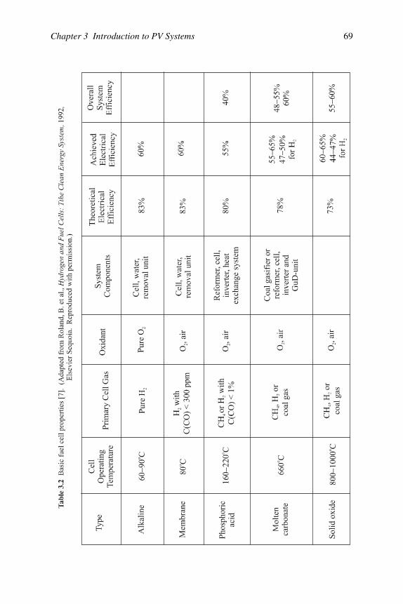
Chapter 3 Introduction to PV Systems 69
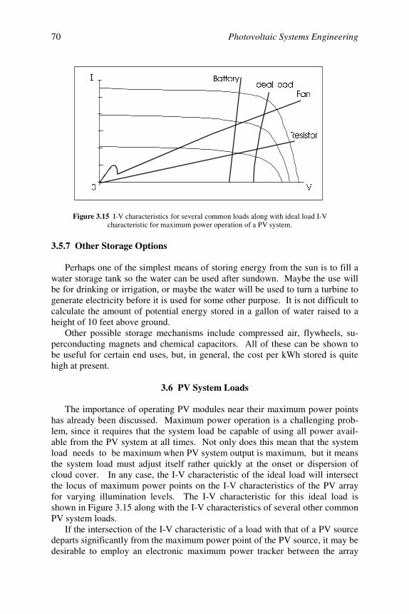
Photovoltaic Systems Engineering70
3.5.7 Other Storage Options
Perhaps one of the simplest means of storing energy from the sun is to fill awater storage tank so the water can be used after sundown. Maybe the use willbe for drinking or irrigation, or maybe the water will be used to turn a turbine togenerate electricity before it is used for some other purpose. It is not difficult tocalculate the amount of potential energy stored in a gallon of water raised to aheight of 10 feet above ground.
Other possible storage mechanisms include compressed air, flywheels, su-perconducting magnets and chemical capacitors. All of these can be shown tobe useful for certain end uses, but, in general, the cost per kWh stored is quitehigh at present.
3.6 PV System Loads
The importance of operating PV modules near their maximum power pointshas already been discussed. Maximum power operation is a challenging prob-lem, since it requires that the system load be capable of using all power avail-able from the PV system at all times. Not only does this mean that the systemload needs to be maximum when PV system output is maximum, but it meansthe system load must adjust itself rather quickly at the onset or dispersion ofcloud cover. In any case, the I-V characteristic of the ideal load will intersectthe locus of maximum power points on the I-V characteristics of the PV arrayfor varying illumination levels. The I-V characteristic for this ideal load isshown in Figure 3.15 along with the I-V characteristics of several other commonPV system loads.
If the intersection of the I-V characteristic of a load with that of a PV sourcedeparts significantly from the maximum power point of the PV source, it may bedesirable to employ an electronic maximum power tracker between the array
,
9
,GHDOORDG%DWWHU\
)DQ
5HVLVWRU
Figure 3.15 I-V characteristics for several common loads along with ideal load I-Vcharacteristic for maximum power operation of a PV system.
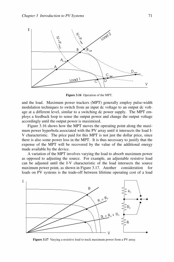
Chapter 3 Introduction to PV Systems 71
and the load. Maximum power trackers (MPT) generally employ pulse-widthmodulation techniques to switch from an input dc voltage to an output dc volt-age at a different level, similar to a switching dc power supply. The MPT em-ploys a feedback loop to sense the output power and change the output voltageaccordingly until the output power is maximized.
Figure 3.16 shows how the MPT moves the operating point along the maxi-mum power hyperbola associated with the PV array until it intersects the load I-V characteristic. The price paid for this MPT is not just the dollar price, sincethere is also some power loss in the MPT. It is thus necessary to justify that theexpense of the MPT will be recovered by the value of the additional energymade available by the device.
A variation of the MPT involves varying the load to absorb maximum poweras opposed to adjusting the source. For example, an adjustable resistive loadcan be adjusted until the I-V characteristic of the load intersects the sourcemaximum power point, as shown in Figure 3.17. Another consideration forloads on PV systems is the trade-off between lifetime operating cost of a load
/0
PD[
/0
PD[
1
2
1PD[
PD[
PD[
2PD[
Figure 3.16 Operation of the MPT.
,
9
5
5
5
5
5
5
5
5
s
s
s
Figure 3.17 Varying a resistive load to track maximum power from a PV array.
Photovoltaic Systems Engineering72
and initial cost of the load. Often a more efficient load is available at a higherinitial cost. It is then necessary for the PV system designer to perform an eco-nomic analysis of both system options to determine which load is a betterchoice. In particular, the choice between relatively inexpensive first-cost incan-descent lamps and more expensive but more efficient fluorescent lamps involvesan interesting cost analysis. Also, the cost difference between dc refrigeratorsand ac refrigerators is considerable, but the efficiency of the dc units is generallysignificantly higher than the ac units, so the purchase of a $2500 dc refrigeratormay be justified. These considerations will be accounted for in Chapter 5.
3.7 PV System Availability
Critical loads are defined as loads for which power is required at least 99%of the time. Noncritical loads require power for at least 95% of the time. It isimportant to recognize that these definitions involve a statistical distribution ofdowntime over the expected lifetime of the system. In other words, a criticalsystem may have availability during any given month or year of its operationthat may be less than 99%, while it will have availability during other years inexcess of 99%. The 99% figure is considered to be an average over the lifetimeof the system.
The reader is probably familiar with causes of downtime on conventionalgrid-connected systems. Sometimes it is a failure of an electrical generator.Sometimes it is a system overload that requires parts of the system to be shutdown selectively to prevent generator overload. Sometimes a tree falls andbreaks a power line. About every 100 years, an ice storm of the century causeslong-term power outages for millions of utility customers, and sometimes a shortcircuit occurs and causes a circuit breaker to trip. Clearly, many other situationsmay occur that will result in the loss of power.
Photovoltaic systems are subject to similar failure modes. Loose or corrodedconnections, battery failure, controller failure and module failure represent a fewof the things that might go wrong in a PV system. However, a good preventivemaintenance program can keep these failure modes at a minimum.
Photovoltaic systems do have a factor that affects system performance towhich conventional systems are not subjected—unpredictable clou d cover. As aresult of unpredictable cloud cover, it is necessary to provide battery backup notonly for hours of nighttime operation, but for those days when the sun eitherdoes not shine at all or when it shines too little to make sufficient electricity tomeet the required daily need. Most readers are aware that different geographicallocations have different seasons when cloudy days are more common. Thereader in the north will be familiar with the winter weeks when the sun almostnever peeks through the cloud cover. The reader in the south will be familiarwith the rainy summer days when little sun is available. The bottom line is thatfor different geographical locations, different amounts of battery backup arerequired for critical and noncritical loads.
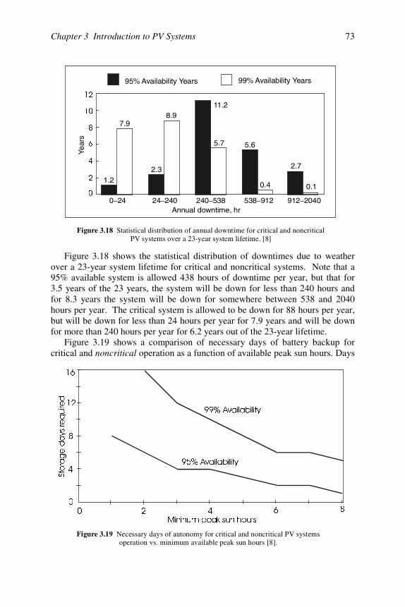
Chapter 3 Introduction to PV Systems 73
Figure 3.18 shows the statistical distribution of downtimes due to weatherover a 23-year system lifetime for critical and noncritical systems. Note that a95% available system is allowed 438 hours of downtime per year, but that for3.5 years of the 23 years, the system will be down for less than 240 hours andfor 8.3 years the system will be down for somewhere between 538 and 2040hours per year. The critical system is allowed to be down for 88 hours per year,but will be down for less than 24 hours per year for 7.9 years and will be downfor more than 240 hours per year for 6.2 years out of the 23-year lifetime.
Figure 3.19 shows a comparison of necessary days of battery backup forcritical and noncritical operation as a function of available peak sun hours. Days
0 24− 24 240− 240 538− 538 912− 912 2040−Annual downtime, hr
Figure 3.18 Statistical distribution of annual downtime for critical and noncriticalPV systems over a 23-year system lifetime. [8]
Year
s95% Availability Years 99% Availability Years
1.2
7.9
2.3
8.911.2
5.7 5.6
0.4
2.7
0.1
0LQLQXPSHDNVXQKRXUV
6WRUDJHGD\VUHTXLUHG
$YDLODELOLW\
$YDLODELOLW\
Figure 3.19 Necessary days of autonomy for critical and noncritical PV systemsoperation vs. minimum available peak sun hours [8].
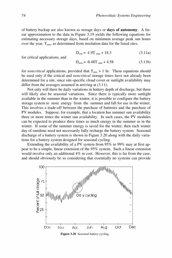
Photovoltaic Systems Engineering74
of battery backup are also known as storage days or days of autonomy. A lin-ear approximation to the data in Figure 3.19 yields the following equations forestimating necessary storage days, based on minimum average peak sun hoursover the year, Tmin, as determined from insolation data for the listed sites.
Dcrit = –1.9T min + 18.3 (3.11a)for critical applications, and
Dnon = –0.48T min + 4.58 (3.11b)
for noncritical applications, provided that Tmin > 1 hr. These equations shouldbe used only if the critical and noncritical storage times have not already beendetermined for a site, since site-specific cloud cover or sunlight availability maydiffer from the averages assumed in arriving at (3.11).
Not only will there be daily variations in battery depth of discharge, but therewill likely also be seasonal variations. Since there is typically more sunlightavailable in the summer than in the winter, it is possible to configure the batterystorage system to store energy from the summer and fall for use in the winter.This involves a trade-off between the purchase of batteries and the purchase ofPV modules. Suppose, for example, that a location has summer sun availabilitythree or more times the winter sun availability. In such cases, the PV modulescan be expected to produce three times as much energy in the summer as in thewinter. If some of the summer energy is saved for the winter, then each winterday of sunshine need not necessarily fully recharge the battery system. Seasonaldischarge of a battery system is shown in Figure 3.20 along with the daily varia-tions for a battery system designed for seasonal cycling.
Extending the availability of a PV system from 95% to 99% may at first ap-pear to be a simple, linear extension of the 95% system. Such a linear extensionwould involve only an additional 4% in cost. However, this is far from the case,and should obviously be so considering that essentially no systems can provide
'HF )HE $SU -XQ $XJ 2FW 'HF
3HUFHQWRIIXOOFKDUJH
'DLO\F\FOLQJ
Figure 3.20 Seasonal battery cycling.
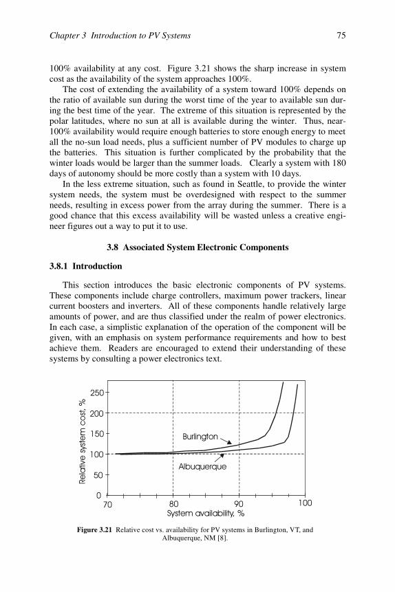
Chapter 3 Introduction to PV Systems 75
100% availability at any cost. Figure 3.21 shows the sharp increase in systemcost as the availability of the system approaches 100%.
The cost of extending the availability of a system toward 100% depends onthe ratio of available sun during the worst time of the year to available sun dur-ing the best time of the year. The extreme of this situation is represented by thepolar latitudes, where no sun at all is available during the winter. Thus, near-100% availability would require enough batteries to store enough energy to meetall the no-sun load needs, plus a sufficient number of PV modules to charge upthe batteries. This situation is further complicated by the probability that thewinter loads would be larger than the summer loads. Clearly a system with 180days of autonomy should be more costly than a system with 10 days.
In the less extreme situation, such as found in Seattle, to provide the wintersystem needs, the system must be overdesigned with respect to the summerneeds, resulting in excess power from the array during the summer. There is agood chance that this excess availability will be wasted unless a creative engi-neer figures out a way to put it to use.
3.8 Associated System Electronic Components
3.8.1 Introduction
This section introduces the basic electronic components of PV systems.These components include charge controllers, maximum power trackers, linearcurrent boosters and inverters. All of these components handle relatively largeamounts of power, and are thus classified under the realm of power electronics.In each case, a simplistic explanation of the operation of the component will begiven, with an emphasis on system performance requirements and how to bestachieve them. Readers are encouraged to extend their understanding of thesesystems by consulting a power electronics text.
Figure 3.21 Relative cost vs. availability for PV systems in Burlington, VT, andAlbuquerque, NM [8].
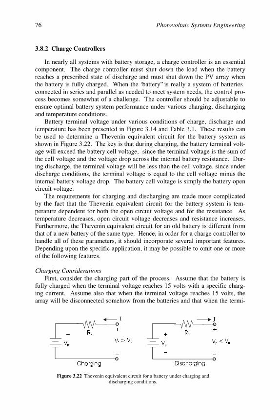
Photovoltaic Systems Engineering76
3.8.2 Charge Controllers
In nearly all systems with battery storage, a charge controller is an essentialcomponent. The charge controller must shut down the load when the batteryreaches a prescribed state of discharge and must shut down the PV array whenthe battery is fully charged. When the “battery” is really a system of batteriesconnected in series and parallel as needed to meet system needs, the control pro-cess becomes somewhat of a challenge. The controller should be adjustable toensure optimal battery system performance under various charging, dischargingand temperature conditions.
Battery terminal voltage under various conditions of charge, discharge andtemperature has been presented in Figure 3.14 and Table 3.1. These results canbe used to determine a Thevenin equivalent circuit for the battery system asshown in Figure 3.22. The key is that during charging, the battery terminal volt-age will exceed the battery cell voltage, since the terminal voltage is the sum ofthe cell voltage and the voltage drop across the internal battery resistance. Dur-ing discharge, the terminal voltage will be less than the cell voltage, since underdischarge conditions, the terminal voltage is equal to the cell voltage minus theinternal battery voltage drop. The battery cell voltage is simply the battery opencircuit voltage.
The requirements for charging and discharging are made more complicatedby the fact that the Thevenin equivalent circuit for the battery system is tem-perature dependent for both the open circuit voltage and for the resistance. Astemperature decreases, open circuit voltage decreases and resistance increases.Furthermore, the Thevenin equivalent circuit for an old battery is different fromthat of a new battery of the same type. Hence, in order for a charge controller tohandle all of these parameters, it should incorporate several important features.Depending upon the specific application, it may be possible to omit one or moreof the following features.
Charging ConsiderationsFirst, consider the charging part of the process. Assume that the battery is
fully charged when the terminal voltage reaches 15 volts with a specific charg-ing current. Assume also that when the terminal voltage reaches 15 volts, thearray will be disconnected somehow from the batteries and that when the termi-
9% 9
%
5%
5%
B B
B B
97 9
79
%!9
%
, ,
&KDUJLQJ 'LVFKDUJLQJ
Figure 3.22 Thevenin equivalent circuit for a battery under charging anddischarging conditions.
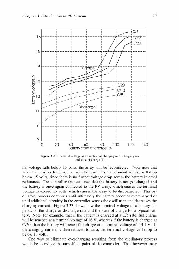
Chapter 3 Introduction to PV Systems 77
nal voltage falls below 15 volts, the array will be reconnected. Now note thatwhen the array is disconnected from the terminals, the terminal voltage will dropbelow 15 volts, since there is no further voltage drop across the battery internalresistance. The controller thus assumes that the battery is not yet charged andthe battery is once again connected to the PV array, which causes the terminalvoltage to exceed 15 volts, which causes the array to be disconnected. This os-cillatory process continues until ultimately the battery becomes overcharged oruntil additional circuitry in the controller senses the oscillation and decreases thecharging current. Figure 3.23 shows how the terminal voltage of a battery de-pends on the charge or discharge rate and the state of charge for a typical bat-tery. Note, for example, that if the battery is charged at a C/5 rate, full chargewill be reached at a terminal voltage of 16 V, whereas if the battery is charged atC/20, then the battery will reach full charge at a terminal voltage of 14.1 V. Ifthe charging current is then reduced to zero, the terminal voltage will drop tobelow 13 volts.
One way to eliminate overcharging resulting from the oscillatory processwould be to reduce the turnoff set point of the controller. This, however, may
Figure 3.23 Terminal voltage as a function of charging or discharging rateand state of charge [1].
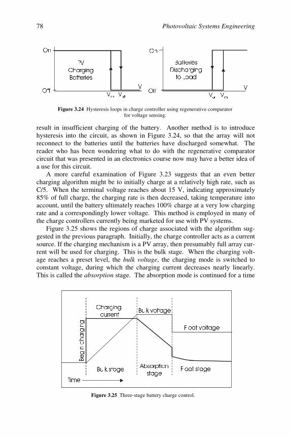
Photovoltaic Systems Engineering78
result in insufficient charging of the battery. Another method is to introducehysteresis into the circuit, as shown in Figure 3.24, so that the array will notreconnect to the batteries until the batteries have discharged somewhat. Thereader who has been wondering what to do with the regenerative comparatorcircuit that was presented in an electronics course now may have a better idea ofa use for this circuit.
A more careful examination of Figure 3.23 suggests that an even bettercharging algorithm might be to initially charge at a relatively high rate, such asC/5. When the terminal voltage reaches about 15 V, indicating approximately85% of full charge, the charging rate is then decreased, taking temperature intoaccount, until the battery ultimately reaches 100% charge at a very low chargingrate and a correspondingly lower voltage. This method is employed in many ofthe charge controllers currently being marketed for use with PV systems.
Figure 3.25 shows the regions of charge associated with the algorithm sug-gested in the previous paragraph. Initially, the charge controller acts as a currentsource. If the charging mechanism is a PV array, then presumably full array cur-rent will be used for charging. This is the bulk stage. When the charging volt-age reaches a preset level, the bulk voltage, the charging mode is switched toconstant voltage, during which the charging current decreases nearly linearly.This is called the absorption stage. The absorption mode is continued for a time
2Q 2Q
2II 2II9
7 97
39
&KDUJLQJ
%DWWHULHV
9RII 9
RII9
RQ 9RQ
%DWWHULHV
'LVFKDUJLQJ
WR/RDG
Figure 3.24 Hysteresis loops in charge controller using regenerative comparatorfor voltage sensing.
&KDUJLQJ
FXUUHQW
7LPH
%XONVWDJH$EVRUSWLRQ
VWDJH)ORDWVWDJH
%XONYROWDJH
)ORDWYROWDJH
Figure 3.25 Three-stage battery charge control.
%HJLQFKDUJLQJ
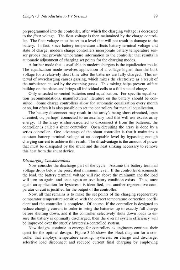
Chapter 3 Introduction to PV Systems 79
preprogrammed into the controller, after which the charging voltage is decreasedto the float voltage. The float voltage is then maintained by the charge control-ler. The float voltage must be set to a level that will not result in damage to thebattery. In fact, since battery temperature affects battery terminal voltage andstate of charge, modern charge controllers incorporate battery temperature sen-sor probes that provide temperature information to the controller that results inautomatic adjustment of charging set points for the charging modes.
A further mode that is available in modern chargers is the equalization mode.The equalization mode involves application of a voltage higher than the bulkvoltage for a relatively short time after the batteries are fully charged. This in-terval of overcharging causes gassing, which mixes the electrolyte as a result ofthe turbulence caused by the escaping gases. This mixing helps prevent sulfatebuildup on the plates and brings all individual cells to a full state of charge.
Only unsealed or vented batteries need equalization. For specific equaliza-tion recommendations, manufacturers’ literature on the battery should be con-sulted. Some charge controllers allow for automatic equalization every monthor so, but often it is also possible to set the controllers for manual equalization.
The battery disconnect may result in the array’s being short-circuited, opencircuited, or, perhaps, connected to an auxiliary load that will use excess arrayenergy. If the array is short-circuited to disconnect it from the batteries, thecontroller is called a shunt controller. Open circuiting the array is done by aseries controller. One advantage of the shunt controller is that it maintains aconstant battery terminal voltage at an acceptable level by bypassing enoughcharging current to achieve this result. The disadvantage is the amount of powerthat must be dissipated by the shunt and the heat sinking necessary to removethis heat from the shunt device.
Discharging ConsiderationsNow consider the discharge part of the cycle. Assume the battery terminal
voltage drops below the prescribed minimum level. If the controller disconnectsthe load, the battery terminal voltage will rise above the minimum and the loadwill turn on again, and once again an oscillatory condition exists. Thus, onceagain an application for hysteresis is identified, and another regenerative com-parator circuit is justified for the output of the controller.
Now, all that remains is to make the set points of the charging regenerativecomparator temperature sensitive with the correct temperature correction coeffi-cient and the controller is complete. Of course, if the controller is designed toreduce charging current in order to bring the batteries up to exactly full chargebefore shutting down, and if the controller selectively shuts down loads to en-sure the battery is optimally discharged, then the overall system efficiency willbe improved over the strictly hysteresis-controlled system.
New designs continue to emerge for controllers as engineers continue theirquest for the optimal design. Figure 3.26 shows the block diagram for a con-troller that employs temperature sensing, hysteresis on charge and discharge,selective load disconnect and reduced current final charging by employing
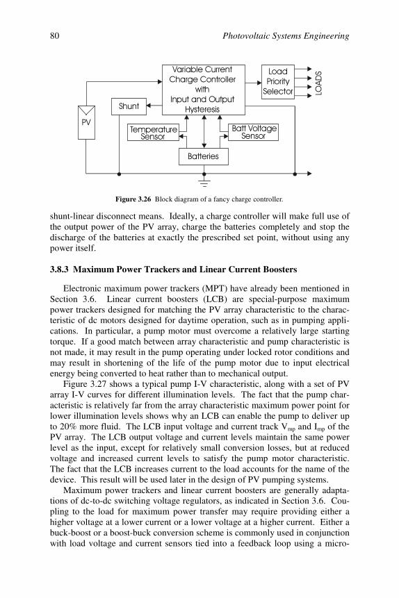
Photovoltaic Systems Engineering80
shunt-linear disconnect means. Ideally, a charge controller will make full use ofthe output power of the PV array, charge the batteries completely and stop thedischarge of the batteries at exactly the prescribed set point, without using anypower itself.
3.8.3 Maximum Power Trackers and Linear Current Boosters
Electronic maximum power trackers (MPT) have already been mentioned inSection 3.6. Linear current boosters (LCB) are special-purpose maximumpower trackers designed for matching the PV array characteristic to the charac-teristic of dc motors designed for daytime operation, such as in pumping appli-cations. In particular, a pump motor must overcome a relatively large startingtorque. If a good match between array characteristic and pump characteristic isnot made, it may result in the pump operating under locked rotor conditions andmay result in shortening of the life of the pump motor due to input electricalenergy being converted to heat rather than to mechanical output.
Figure 3.27 shows a typical pump I-V characteristic, along with a set of PVarray I-V curves for different illumination levels. The fact that the pump char-acteristic is relatively far from the array characteristic maximum power point forlower illumination levels shows why an LCB can enable the pump to deliver upto 20% more fluid. The LCB input voltage and current track Vmp and Imp of thePV array. The LCB output voltage and current levels maintain the same powerlevel as the input, except for relatively small conversion losses, but at reducedvoltage and increased current levels to satisfy the pump motor characteristic.The fact that the LCB increases current to the load accounts for the name of thedevice. This result will be used later in the design of PV pumping systems.
Maximum power trackers and linear current boosters are generally adapta-tions of dc-to-dc switching voltage regulators, as indicated in Section 3.6. Cou-pling to the load for maximum power transfer may require providing either ahigher voltage at a lower current or a lower voltage at a higher current. Either abuck-boost or a boost-buck conversion scheme is commonly used in conjunctionwith load voltage and current sensors tied into a feedback loop using a micro-
!"#
$%& "!#
!#
' ( !
)"# #
*+#&" #(,"&"
-
',.
!
Figure 3.26 Block diagram of a fancy charge controller.
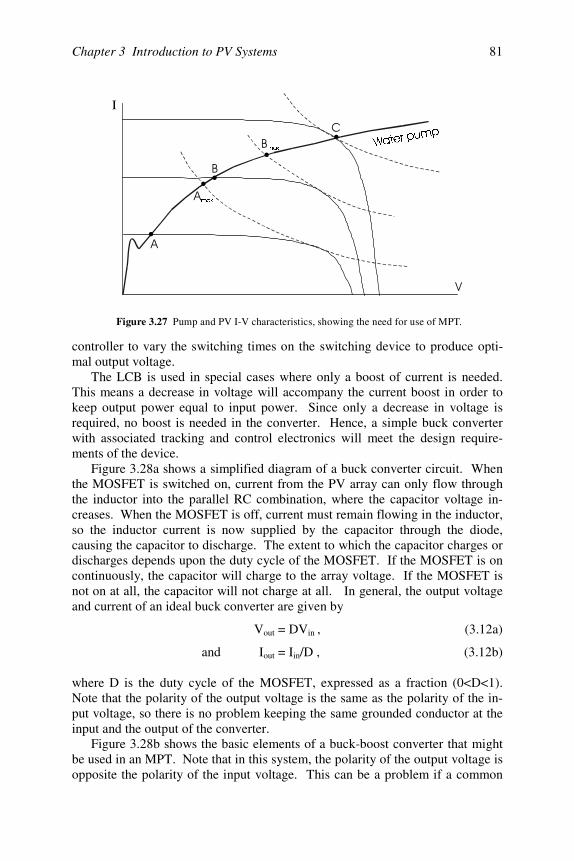
Chapter 3 Introduction to PV Systems 81
controller to vary the switching times on the switching device to produce opti-mal output voltage.
The LCB is used in special cases where only a boost of current is needed.This means a decrease in voltage will accompany the current boost in order tokeep output power equal to input power. Since only a decrease in voltage isrequired, no boost is needed in the converter. Hence, a simple buck converterwith associated tracking and control electronics will meet the design require-ments of the device.
Figure 3.28a shows a simplified diagram of a buck converter circuit. Whenthe MOSFET is switched on, current from the PV array can only flow throughthe inductor into the parallel RC combination, where the capacitor voltage in-creases. When the MOSFET is off, current must remain flowing in the inductor,so the inductor current is now supplied by the capacitor through the diode,causing the capacitor to discharge. The extent to which the capacitor charges ordischarges depends upon the duty cycle of the MOSFET. If the MOSFET is oncontinuously, the capacitor will charge to the array voltage. If the MOSFET isnot on at all, the capacitor will not charge at all. In general, the output voltageand current of an ideal buck converter are given by
Vout = DVin , (3.12a)
and Iout = Iin/D , (3.12b)
where D is the duty cycle of the MOSFET, expressed as a fraction (0<D<1).Note that the polarity of the output voltage is the same as the polarity of the in-put voltage, so there is no problem keeping the same grounded conductor at theinput and the output of the converter. Figure 3.28b shows the basic elements of a buck-boost converter that mightbe used in an MPT. Note that in this system, the polarity of the output voltage isopposite the polarity of the input voltage. This can be a problem if a common
.
PD[
.PD[
:DWHUSXPS
Figure 3.27 Pump and PV I-V characteristics, showing the need for use of MPT.
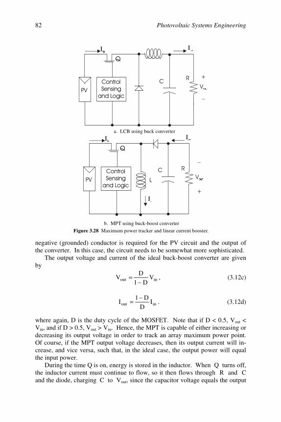
Photovoltaic Systems Engineering82
negative (grounded) conductor is required for the PV circuit and the output ofthe converter. In this case, the circuit needs to be somewhat more sophisticated.
The output voltage and current of the ideal buck-boost converter are givenby
inout VD1
DV
−= , (3.12c)
inout ID
D1I
−= . (3.12d)
where again, D is the duty cycle of the MOSFET. Note that if D < 0.5, Vout <Vin, and if D > 0.5, Vout > Vin. Hence, the MPT is capable of either increasing ordecreasing its output voltage in order to track an array maximum power point.Of course, if the MPT output voltage decreases, then its output current will in-crease, and vice versa, such that, in the ideal case, the output power will equalthe input power.
During the time Q is on, energy is stored in the inductor. When Q turns off,the inductor current must continue to flow, so it then flows through R and Cand the diode, charging C to Vout, since the capacitor voltage equals the output
Figure 3.28 Maximum power tracker and linear current booster.
#!##
#(' '
/
0
1
RXW
LQ
RXW
V
2
b. MPT using buck-boost converter
#!##
#('
/
0
1
RXW
LQ
RXW
2
a. LCB using buck converter
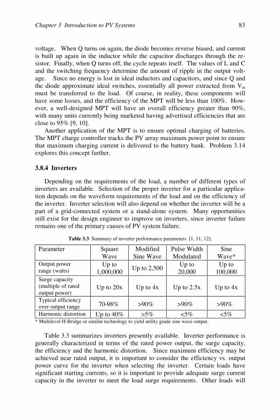
Chapter 3 Introduction to PV Systems 83
voltage. When Q turns on again, the diode becomes reverse biased, and currentis built up again in the inductor while the capacitor discharges through the re-sistor. Finally, when Q turns off, the cycle repeats itself. The values of L and Cand the switching frequency determine the amount of ripple in the output volt-age. Since no energy is lost in ideal inductors and capacitors, and since Q andthe diode approximate ideal switches, essentially all power extracted from Vin
must be transferred to the load. Of course, in reality, these components willhave some losses, and the efficiency of the MPT will be less than 100%. How-ever, a well-designed MPT will have an overall efficiency greater than 90%,with many units currently being marketed having advertised efficiencies that areclose to 95% [9, 10].
Another application of the MPT is to ensure optimal charging of batteries.The MPT charge controller tracks the PV array maximum power point to ensurethat maximum charging current is delivered to the battery bank. Problem 3.14explores this concept further.
3.8.4 Inverters
Depending on the requirements of the load, a number of different types ofinverters are available. Selection of the proper inverter for a particular applica-tion depends on the waveform requirements of the load and on the efficiency ofthe inverter. Inverter selection will also depend on whether the inverter will be apart of a grid-connected system or a stand-alone system. Many opportunitiesstill exist for the design engineer to improve on inverters, since inverter failureremains one of the primary causes of PV system failure.
Table 3.3 Summary of inverter performance parameters [1, 11, 12].
Parameter SquareWave
ModifiedSine Wave
Pulse WidthModulated
SineWave*
Output powerrange (watts)
Up to1,000,000
Up to 2,500Up to
20,000Up to
100,000Surge capacity(multiple of ratedoutput power)
Up to 20x Up to 4x Up to 2.5x Up to 4x
Typical efficiencyover output range 70–98% >90% >90% >90%
Harmonic distortion Up to 40% >5% <5% <5%* Multilevel H-Bridge or similar technology to yield utility grade sine wave output.
Table 3.3 summarizes inverters presently available. Inverter performance isgenerally characterized in terms of the rated power output, the surge capacity,the efficiency and the harmonic distortion. Since maximum efficiency may beachieved near rated output, it is important to consider the efficiency vs. outputpower curve for the inverter when selecting the inverter. Certain loads havesignificant starting currents, so it is important to provide adequate surge currentcapacity in the inverter to meet the load surge requirements. Other loads will
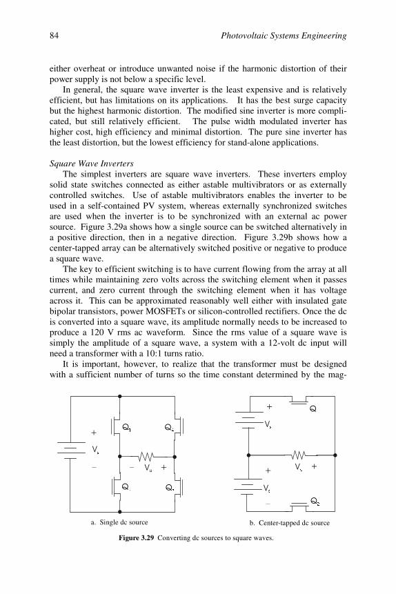
Photovoltaic Systems Engineering84
either overheat or introduce unwanted noise if the harmonic distortion of theirpower supply is not below a specific level.
In general, the square wave inverter is the least expensive and is relativelyefficient, but has limitations on its applications. It has the best surge capacitybut the highest harmonic distortion. The modified sine inverter is more compli-cated, but still relatively efficient. The pulse width modulated inverter hashigher cost, high efficiency and minimal distortion. The pure sine inverter hasthe least distortion, but the lowest efficiency for stand-alone applications.
Square Wave InvertersThe simplest inverters are square wave inverters. These inverters employ
solid state switches connected as either astable multivibrators or as externallycontrolled switches. Use of astable multivibrators enables the inverter to beused in a self-contained PV system, whereas externally synchronized switchesare used when the inverter is to be synchronized with an external ac powersource. Figure 3.29a shows how a single source can be switched alternatively ina positive direction, then in a negative direction. Figure 3.29b shows how acenter-tapped array can be alternatively switched positive or negative to producea square wave.
The key to efficient switching is to have current flowing from the array at alltimes while maintaining zero volts across the switching element when it passescurrent, and zero current through the switching element when it has voltageacross it. This can be approximated reasonably well either with insulated gatebipolar transistors, power MOSFETs or silicon-controlled rectifiers. Once the dcis converted into a square wave, its amplitude normally needs to be increased toproduce a 120 V rms ac waveform. Since the rms value of a square wave issimply the amplitude of a square wave, a system with a 12-volt dc input willneed a transformer with a 10:1 turns ratio.
It is important, however, to realize that the transformer must be designedwith a sufficient number of turns so the time constant determined by the mag-
2
2
2
2
2
21
0
V
V
V
R
R1 10 0
1
1
0
0
a. Single dc source b. Center-tapped dc source
Figure 3.29 Converting dc sources to square waves.

Chapter 3 Introduction to PV Systems 85
netizing inductance of the transformer and the source resistance will be longenough to maintain the square wave. Too few turns on the transformer willcause the output waveform to droop as shown in Figure 3.30. When specifyingthe transformer for this application, it is easy to assume that transformers areideal and to simply try to use a 120:12 volt transformer backwards. The 120:12volt transformer, however, probably would have been designed for use with asinusoidal signal, and thus would not have enough turns to handle the squarewave effectively. A square wave inverter with a good transformer and efficientswitching can operate at efficiencies in the 90% range.
Modified Sine Wave InvertersFor a number of applications, a square wave is inadequate for meeting the
harmonic distortion requirements of the load. For example, since square waveshave significant harmonic content, and since hysteresis and eddy current lossesin magnetic materials increase significantly with increase in frequency, squarewave excitation may cause some motors or fluorescent ballasts to overheat.
Square wave harmonics can also introduce noise into a system. Thus, beforeselecting an inverter, it is important to verify that the proposed load will operatewith square wave excitation.
If square wave excitation is not suitable for a load, it is possible that a modi-fied sine wave will work. A number of methods are available to convert theoutput of a dc source into some approximation of a sine wave. One such methodinvolves using a multilevel H-bridge as shown in Figure 3.31a to generate awaveform such as the one shown in Figure 3.31b. The idea is to time the indi-vidual voltage levels so that harmonic distortion will be minimized and that therms value of the output voltage will remain constant in the event that the inputdc voltage should vary.
The sequence for closing switches to obtain portions of the waveform inFigure 3.31b is shown on the waveform diagram. The actual switches may bebipolar transistors, MOS transistors, SCRs or insulated gate bipolar transistors.As an example of how the various voltage levels in vo are obtained, consider theinterval T1, where, according to the output voltage waveform, vo = 0.5Vdc. If S1
Figure 3.30 Output waveforms for square wave inverter with adequate and with inadequate number of transformer turns.
a. Adequate b. Inadequate
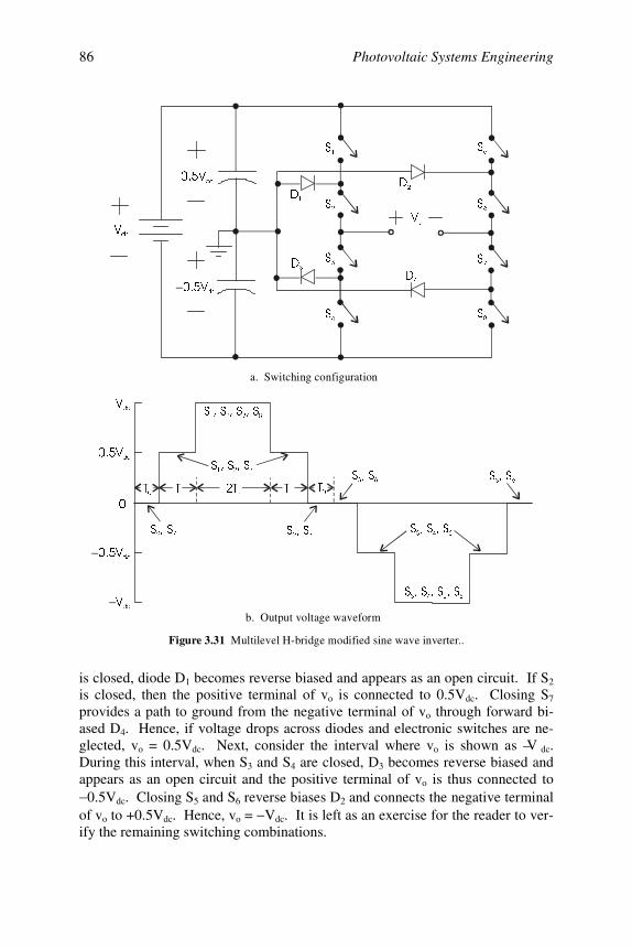
Photovoltaic Systems Engineering86
is closed, diode D1 becomes reverse biased and appears as an open circuit. If S2
is closed, then the positive terminal of vo is connected to 0.5Vdc. Closing S7
provides a path to ground from the negative terminal of vo through forward bi-ased D4. Hence, if voltage drops across diodes and electronic switches are ne-glected, vo = 0.5Vdc. Next, consider the interval where vo is shown as –V dc.During this interval, when S3 and S4 are closed, D3 becomes reverse biased andappears as an open circuit and the positive terminal of vo is thus connected to−0.5Vdc. Closing S5 and S6 reverse biases D2 and connects the negative terminalof vo to +0.5Vdc. Hence, vo = −Vdc. It is left as an exercise for the reader to ver-ify the remaining switching combinations.
Figure 3.31 Multilevel H-bridge modified sine wave inverter..
a. Switching configuration
b. Output voltage waveform
9GF
9GF
−9GF
−9GF
6 6 6 6
6 6 6
6 6 6 6
6 6 6 6
6 6 6
6 6 6 6
7
77
7
7
9GF
9GF
−9GF
9R
6
6
6
6
6
6
6
6
'
'
'
'
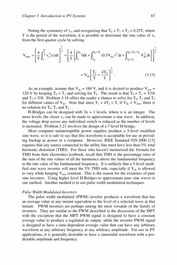
Chapter 3 Introduction to PV Systems 87
Noting the symmetry of vo, and recognizing that T0 + T1 + T2 = 0.25T, whereT is the period of the waveform, it is possible to determine the rms value of vo
from the first quarter cycle by solving
2
1
T TT TTT2dc
2dc
2
1
4
T2orms
0
0
10
0T
210
1T0T0
dtVdt)V5.0(dt0T
4dt)t(v
T
4V
++=
= ∫ ∫ ∫∫
+ ++
+
2
1
21dc T
T4
T
TV
+= . (3.13)
As an example, assume that Vdc = 160 V, and it is desired to produce Vrms =120 V by keeping T0 = T1 and solving for T2. The result is that T0 = T1 = T/16and T2 = T/8. Problem 3.18 offers the reader a chance to solve for T0, T1 and T2
for different values of Vdc. Note that since T1 + 4T2 < T, if Vdc < Vrms, there isno solution for T0, T1 and T2.
H-Bridges can be designed with 2n + 1 levels, where n is an integer. Themore levels, the closer vo can be made to approximate a sine wave. In addition,the voltage drop across any individual switch is reduced as the number of levelsis increased. Problem 3.21 involves the design of a 7-level H-bridge.
Most computer uninterruptible power supplies produce a 5-level modifiedsine wave, so it is safe to say that this waveform is acceptable for use in provid-ing backup ac power to a computer. However, IEEE Standard 929-2000 [13]requires that any source connected to the utility line must have less than 5% totalharmonic distortion (THD). For those who haven’t memorized the formula forTHD from their electronics textbook, recall that THD is the percentage ratio ofthe sum of the rms values of all the harmonics above the fundamental frequencyto the rms value of the fundamental frequency. It is unlikely that a 5-level modi-fied sine wave inverter will meet the 5% THD rule, especially if Vdc is allowedto vary while keeping Vrms constant. This is the reason for the existence of puresine inverters. Using higher level H-Bridges to approximate pure sine waves isone method. Another method is to use pulse width modulation techniques.
Pulse Width Modulated InvertersThe pulse width modulated (PWM) inverter produces a waveform that has
an average value at any instant equivalent to the level of a selected wave at thatinstant. PWM inverters are perhaps among the most versatile of the family ofinverters. They are similar to the PWM described in the discussion of the MPTwith the exception that the MPT PWM signal is designed to have a constantaverage value to produce a regulated dc output, while the inverter PWM signalis designed to have a time-dependent average value that can have any arbitrarywaveform at any arbitrary frequency at any arbitrary amplitude. For use in PVapplications, it is generally desirable to have a sinusoidal waveform with a pre-dictable amplitude and frequency.
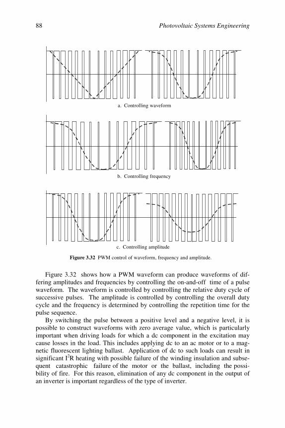
Photovoltaic Systems Engineering88
Figure 3.32 shows how a PWM waveform can produce waveforms of dif-fering amplitudes and frequencies by controlling the on-and-off time of a pulsewaveform. The waveform is controlled by controlling the relative duty cycle ofsuccessive pulses. The amplitude is controlled by controlling the overall dutycycle and the frequency is determined by controlling the repetition time for thepulse sequence.
By switching the pulse between a positive level and a negative level, it ispossible to construct waveforms with zero average value, which is particularlyimportant when driving loads for which a dc component in the excitation maycause losses in the load. This includes applying dc to an ac motor or to a mag-netic fluorescent lighting ballast. Application of dc to such loads can result insignificant I2R heating with possible failure of the winding insulation and subse-quent catastrophic failure of the motor or the ballast, including the possi-bility of fire. For this reason, elimination of any dc component in the output ofan inverter is important regardless of the type of inverter.
a. Controlling waveform
b. Controlling frequency
c. Controlling amplitude
Figure 3.32 PWM control of waveform, frequency and amplitude.
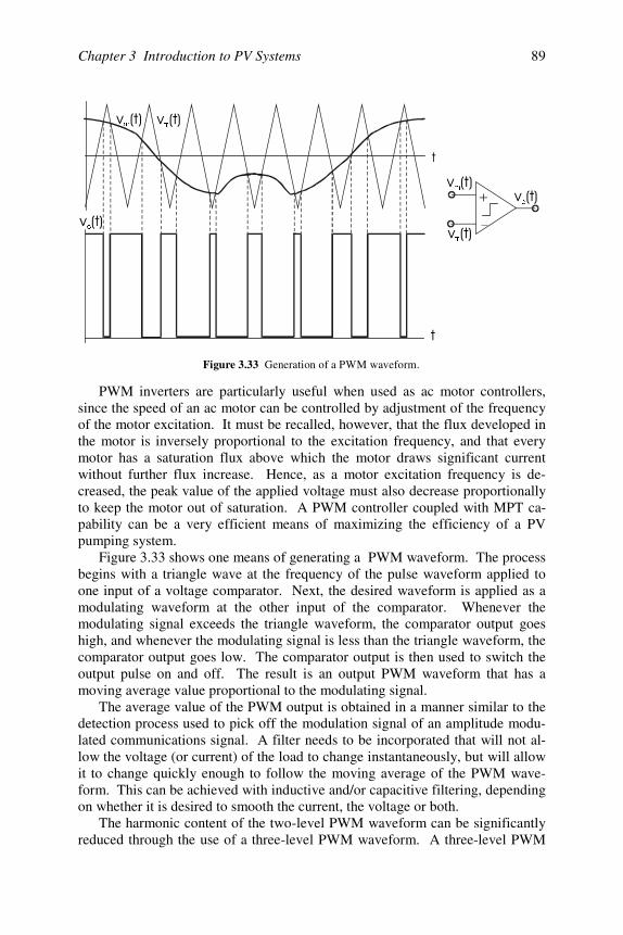
Chapter 3 Introduction to PV Systems 89
PWM inverters are particularly useful when used as ac motor controllers,since the speed of an ac motor can be controlled by adjustment of the frequencyof the motor excitation. It must be recalled, however, that the flux developed inthe motor is inversely proportional to the excitation frequency, and that everymotor has a saturation flux above which the motor draws significant currentwithout further flux increase. Hence, as a motor excitation frequency is de-creased, the peak value of the applied voltage must also decrease proportionallyto keep the motor out of saturation. A PWM controller coupled with MPT ca-pability can be a very efficient means of maximizing the efficiency of a PVpumping system.
Figure 3.33 shows one means of generating a PWM waveform. The processbegins with a triangle wave at the frequency of the pulse waveform applied toone input of a voltage comparator. Next, the desired waveform is applied as amodulating waveform at the other input of the comparator. Whenever themodulating signal exceeds the triangle waveform, the comparator output goeshigh, and whenever the modulating signal is less than the triangle waveform, thecomparator output goes low. The comparator output is then used to switch theoutput pulse on and off. The result is an output PWM waveform that has amoving average value proportional to the modulating signal.
The average value of the PWM output is obtained in a manner similar to thedetection process used to pick off the modulation signal of an amplitude modu-lated communications signal. A filter needs to be incorporated that will not al-low the voltage (or current) of the load to change instantaneously, but will allowit to change quickly enough to follow the moving average of the PWM wave-form. This can be achieved with inductive and/or capacitive filtering, dependingon whether it is desired to smooth the current, the voltage or both.
The harmonic content of the two-level PWM waveform can be significantlyreduced through the use of a three-level PWM waveform. A three-level PWM
34R
WUL
P
R
WUL
P
Figure 3.33 Generation of a PWM waveform.
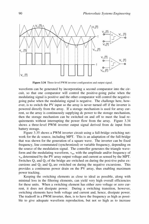
Photovoltaic Systems Engineering90
waveform can be generated by incorporating a second comparator into the cir-cuit, so that one comparator will control the positive-going pulse when themodulating signal is positive and the other comparator will control the negative-going pulse when the modulating signal is negative. The challenge here, how-ever, is to switch the PV input so the array is never turned off if the inverter ispowered directly from the array. If a storage mechanism is used for array cur-rent, so the array is continuously supplying dc power to the storage mechanism,then the storage mechanism can be switched on and off to meet the load re-quirements without interrupting the power flow from the array. Figure 3.34shows a three-level PWM inverter output signal derived from dc input frombattery storage.
Figure 3.35 shows a PWM inverter circuit using a full-bridge switching net-work for the dc source, including MPT. This is an adaptation of the full-bridgethat was shown for the generation of a square wave. The inverter can be fixedfrequency, line commutated (synchronized) or variable frequency, depending onthe source of the modulation signal. The controller generates the triangle wave-form and the modulating waveform, vm, with the amplitude and/or frequency ofvm determined by the PV array output voltage and current as sensed by the MPT.Switches Q1 and Q3 of the bridge are switched on during the posi-tive pulse ex-cursions and Q2 and Q4 are switched on during the negative excursions. Thisprovides a continuous power drain on the PV array, thus enabling maximumpower tracking.
Keeping the switching elements as close to ideal as possible, along withminimal loss in the filtering elements, can yield very high overall efficienciesfor these units. When a switching element has either zero voltage or zero cur-rent, it does not dissipate power. During a switching transition, however,switching elements have both voltage and current and, hence, dissipate power.The tradeoff in a PWM inverter, then, is to have the frequency as high as possi-ble to give adequate waveform reproduction, but not so high as to increase
Figure 3.34 Three-level PWM inverter configuration and output signal.
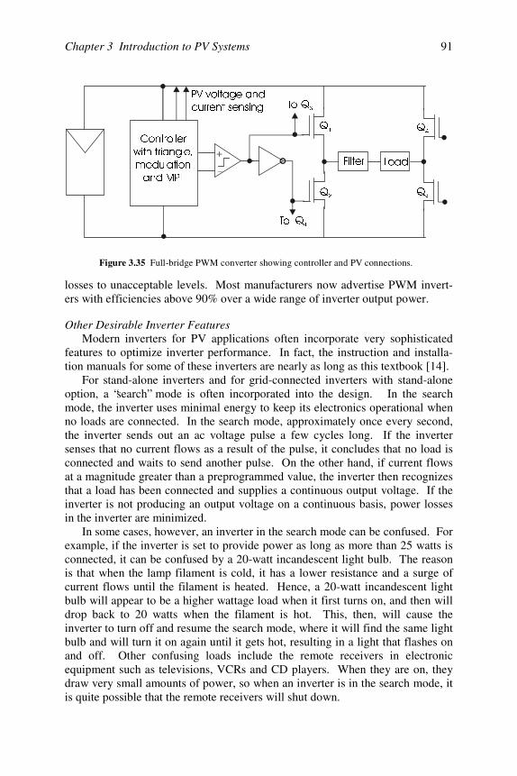
Chapter 3 Introduction to PV Systems 91
losses to unacceptable levels. Most manufacturers now advertise PWM invert-ers with efficiencies above 90% over a wide range of inverter output power.
Other Desirable Inverter FeaturesModern inverters for PV applications often incorporate very sophisticated
features to optimize inverter performance. In fact, the instruction and installa-tion manuals for some of these inverters are nearly as long as this textbook [14].
For stand-alone inverters and for grid-connected inverters with stand-aloneoption, a “search” mode is often incorporated into the design. In the searchmode, the inverter uses minimal energy to keep its electronics operational whenno loads are connected. In the search mode, approximately once every second,the inverter sends out an ac voltage pulse a few cycles long. If the invertersenses that no current flows as a result of the pulse, it concludes that no load isconnected and waits to send another pulse. On the other hand, if current flowsat a magnitude greater than a preprogrammed value, the inverter then recognizesthat a load has been connected and supplies a continuous output voltage. If theinverter is not producing an output voltage on a continuous basis, power lossesin the inverter are minimized.
In some cases, however, an inverter in the search mode can be confused. Forexample, if the inverter is set to provide power as long as more than 25 watts isconnected, it can be confused by a 20-watt incandescent light bulb. The reasonis that when the lamp filament is cold, it has a lower resistance and a surge ofcurrent flows until the filament is heated. Hence, a 20-watt incandescent lightbulb will appear to be a higher wattage load when it first turns on, and then willdrop back to 20 watts when the filament is hot. This, then, will cause theinverter to turn off and resume the search mode, where it will find the same lightbulb and will turn it on again until it gets hot, resulting in a light that flashes onand off. Other confusing loads include the remote receivers in electronicequipment such as televisions, VCRs and CD players. When they are on, theydraw very small amounts of power, so when an inverter is in the search mode, itis quite possible that the remote receivers will shut down.
4
4
4
4
4
4
7R
7R
)LOWHU /RDG
39YROWDJHDQG
FXUUHQWVHQVLQJ
&RQWUROOHU
ZLWKWULDQJOH
PRGXODWLRQ
DQG037
Figure 3.35 Full-bridge PWM converter showing controller and PV connections.
Photovoltaic Systems Engineering92
For stand-alone inverters, it is necessary that the output appear as a voltagesource, preferably as close to ideal as possible. For utility interactive inverters,however, it is more convenient to let the grid voltage fulfill the voltage sourcerole and to have the inverter act as a current source that feeds current into theutility grid. Utility interactive inverters with battery backup that are capable ofsupplying power to emergency loads if the utility grid is disconnected must becapable of switching over from grid-synchronized current source to internallysynchronized voltage source to power emergency loads.
Utility interactive inverters must be designed so that if the utility goes down,the inverter output to the utility also shuts down. This safety feature is relativelyeasy to design into an inverter if no other distributed electrical source is con-nected to the utility. However, if another nonutility source is connected to theline it is important that the PV system inverter will not recognize this source as autility source and continue to supply power to the line. This is called “island-ing” and will be discussed later in this chapter and also in Ch apter 8.
Many utility interactive inverters that have an emergency backup feature alsoincorporate a battery charger in the inverter so the utility can be used to chargethe batteries in the event that the PV system has not fully charged the batteries.This feature only works, of course, when the utility grid is energized. Fortu-nately, this is generally most of the time.
Another convenient feature found in many inverters is a generator start op-tion. This allows for a separate ac generator to be used as a backup to the PVsystem in either a utility interactive or a stand-alone system. When the batterylevel of charge drops to a prescribed level, the inverter will send a starting signalto the generator. If the inverter has a real-time clock, the time of day for gen-erator starting can also be controlled, so the generator will not come on just be-fore the sun is about to charge the batteries.
Finally, most high quality inverters that are connected to a PV array willincorporate maximum power tracking circuitry at their dc input so that the PVarray will deliver power at its maximum power level to the inverter.
3.9 Generators
3.9.1 Introduction
In some cases, where either a large discrepancy between seasonal loads ex-ists or where seasonal sun availability varies greatly, a system designed com-pletely around PV components will result in the deployment of a large PV arrayto meet the needs of one season. Meanwhile, during other seasons, much of theenergy available from the array is not used. This is similar to the problem ofmeeting critical system needs with PV, where the cost generally increases rap-idly as the system availability exceeds 95%. In such cases, it is often more costeffective to employ an alternate source of electricity to be available when the PVarray is not meeting system needs. While it is conceivable that the backupsource for a stand-alone system may be wind or other renewable source, it is
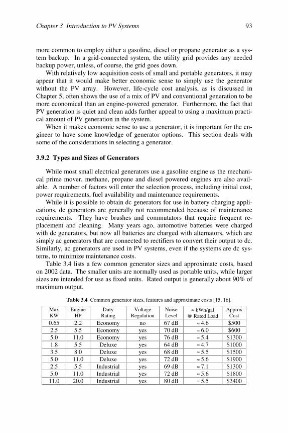
Chapter 3 Introduction to PV Systems 93
more common to employ either a gasoline, diesel or propane generator as a sys-tem backup. In a grid-connected system, the utility grid provides any neededbackup power, unless, of course, the grid goes down.
With relatively low acquisition costs of small and portable generators, it mayappear that it would make better economic sense to simply use the generatorwithout the PV array. However, life-cycle cost analysis, as is discussed inChapter 5, often shows the use of a mix of PV and conventional generation to bemore economical than an engine-powered generator. Furthermore, the fact thatPV generation is quiet and clean adds further appeal to using a maximum practi-cal amount of PV generation in the system.
When it makes economic sense to use a generator, it is important for the en-gineer to have some knowledge of generator options. This section deals withsome of the considerations in selecting a generator.
3.9.2 Types and Sizes of Generators
While most small electrical generators use a gasoline engine as the mechani-cal prime mover, methane, propane and diesel powered engines are also avail-able. A number of factors will enter the selection process, including initial cost,power requirements, fuel availability and maintenance requirements.
While it is possible to obtain dc generators for use in battery charging appli-cations, dc generators are generally not recommended because of maintenancerequirements. They have brushes and commutators that require frequent re-placement and cleaning. Many years ago, automotive batteries were chargedwith dc generators, but now all batteries are charged with alternators, which aresimply ac generators that are connected to rectifiers to convert their output to dc.Similarly, ac generators are used in PV systems, even if the systems are dc sys-tems, to minimize maintenance costs. Table 3.4 lists a few common generator sizes and approximate costs, basedon 2002 data. The smaller units are normally used as portable units, while largersizes are intended for use as fixed units. Rated output is generally about 90% ofmaximum output.
Table 3.4 Common generator sizes, features and approximate costs [15, 16].
MaxKW
EngineHP
DutyRating
VoltageRegulation
NoiseLevel
≈ kWh/gal@ Rated Load
ApproxCost
0.65 2.2 Economy no 67 dB ≈ 4.6 $5002.5 5.5 Economy yes 70 dB ≈ 6.0 $6005.0 11.0 Economy yes 76 dB ≈ 5.4 $13001.8 5.5 Deluxe yes 64 dB ≈ 4.7 $10003.5 8.0 Deluxe yes 68 dB ≈ 5.5 $15005.0 11.0 Deluxe yes 72 dB ≈ 5.6 $19002.5 5.5 Industrial yes 69 dB ≈ 7.1 $13005.0 11.0 Industrial yes 72 dB ≈ 5.6 $180011.0 20.0 Industrial yes 80 dB ≈ 5.5 $3400
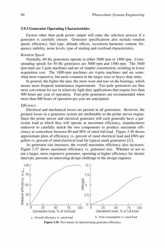
Photovoltaic Systems Engineering94
3.9.3 Generator Operating Characteristics
Factors other than peak power output will enter the selection process if agenerator is carefully chosen. Generator specifications also include rotationspeed, efficiency, fuel type, altitude effects, waveform harmonic content, fre-quency stability, noise levels, type of starting and overload characteristics.
Rotation SpeedNormally, 60 Hz generators operate at either 3600 rpm or 1800 rpm. Corre-
sponding speeds for 50 Hz generators are 3000 rpm and 1500 rpm. The 3600rpm units are 2-pole machines and are of simpler construction, resulting in loweracquisition cost. The 1800-rpm machines are 4-pole machines and are some-what more expensive, but more common in the larger sizes or heavy duty units.
In general, the higher the rpm, the more wear and tear on the bearings, whichmeans more frequent maintenance requirements. Two-pole generators are thusmost convenient for use in relatively light duty applications that require less than400 hours per year of operation. Four-pole generators are recommended whenmore than 400 hours of operation per year are anticipated.
EfficiencyElectrical and mechanical losses are present in all generators. However, the
greatest losses in a generator system are attributable to the prime mover engine.Since the prime mover and electrical generator will each generally have a par-ticular load at which they will operate at maximum efficiency, manufacturersendeavor to carefully match the two components to produce maximum effi-ciency at somewhere between 80 and 90% of rated full load. Figure 3.36 showsapproximate plots of efficiency vs. percent of rated electrical load and kWh pergallon vs. percent of rated electrical load for typical small generators [21].
As generator size increases, the overall maximum efficiency also increases.Figure 3.37 shows maximum efficiency vs. generator size. Whether or not touse a larger, more expensive generator, operating at higher efficiency for shorterintervals, presents an interesting design challenge to the design engineer.
Figure 3.36 Two means of characterizing generator efficiency.
a. Overall efficiency vs. rated load. b. Fuel consumption vs. rated load
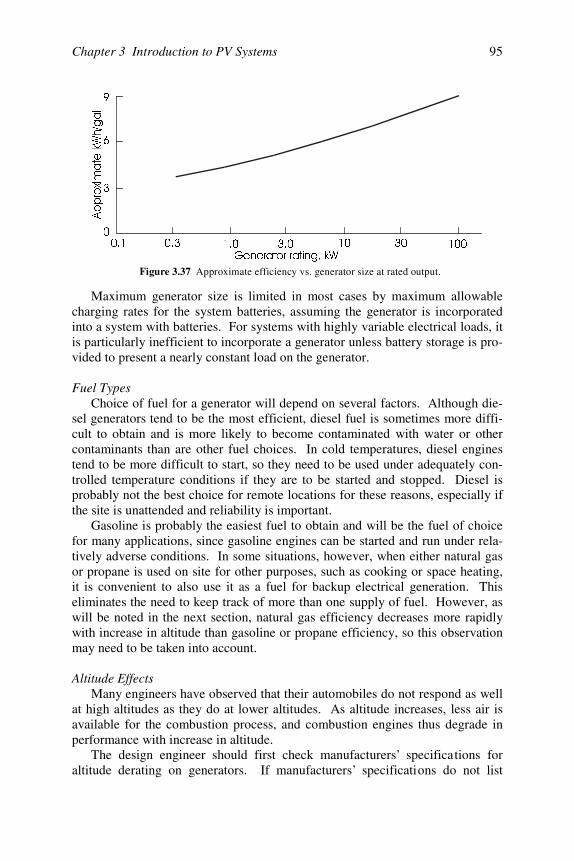
Chapter 3 Introduction to PV Systems 95
Maximum generator size is limited in most cases by maximum allowablecharging rates for the system batteries, assuming the generator is incorporatedinto a system with batteries. For systems with highly variable electrical loads, itis particularly inefficient to incorporate a generator unless battery storage is pro-vided to present a nearly constant load on the generator.
Fuel TypesChoice of fuel for a generator will depend on several factors. Although die-
sel generators tend to be the most efficient, diesel fuel is sometimes more diffi-cult to obtain and is more likely to become contaminated with water or othercontaminants than are other fuel choices. In cold temperatures, diesel enginestend to be more difficult to start, so they need to be used under adequately con-trolled temperature conditions if they are to be started and stopped. Diesel isprobably not the best choice for remote locations for these reasons, especially ifthe site is unattended and reliability is important.
Gasoline is probably the easiest fuel to obtain and will be the fuel of choicefor many applications, since gasoline engines can be started and run under rela-tively adverse conditions. In some situations, however, when either natural gasor propane is used on site for other purposes, such as cooking or space heating,it is convenient to also use it as a fuel for backup electrical generation. Thiseliminates the need to keep track of more than one supply of fuel. However, aswill be noted in the next section, natural gas efficiency decreases more rapidlywith increase in altitude than gasoline or propane efficiency, so this observationmay need to be taken into account.
Altitude EffectsMany engineers have observed that their automobiles do not respond as well
at high altitudes as they do at lower altitudes. As altitude increases, less air isavailable for the combustion process, and combustion engines thus degrade inperformance with increase in altitude.
The design engineer should first check manufacturers’ specifications foraltitude derating on generators. If manufacturers’ specifications do not list
*HQHUDWRUUDWLQJN:
$SSUR[LPDWHN:KJDO
Figure 3.37 Approximate efficiency vs. generator size at rated output.
Photovoltaic Systems Engineering96
derating factors, then it is reasonable to derate gasoline, diesel and propane gen-erators by 3% per 1000 ft of altitude above sea level and to derate natural gasengines by 5% per 1000 ft of altitude above sea level.
Waveform Harmonic ContentGenerally the output waveform of an electrical generator is adequate for
nearly all applications. For battery charging, almost any waveform is satisfac-tory, depending on whether the battery charger contains a transformer.
If the charger contains a transformer, there is a remote possibility that exces-sive dc or harmonic content in the generator waveform may damage the trans-former. If the generator is connected directly to the PV system ac loads at anytime, then it is a good idea to be sure the generator output waveform is suffi-ciently “clean” to meet the requirements of the loads. Normall y, the only loadswith possible sensitivity to waveform quality will be electronic systems.
Frequency StabilityAgain, depending on load requirements and whether the generator is con-
nected to ac loads with critical power frequency requirements, the frequencystability of a generator may need to be taken into account. It is generally desir-able to maintain frequency fluctuations at less than ± 0.5 Hz for ac loads, butthis degree of frequency stability is not necessary for many PV system loads.
Amplitude StabilityIt is generally desirable to have the generator output voltage amplitude re-
main within 5% of its no-load value. This implies a voltage regulation figure of5%. Depending on whether the load is inductive or capacitive, the load voltageunder full-load conditions may actually exceed the no-load voltage. The voltageregulation of the generator is defined by
fl
flnl
V
VVVR
−= , (3.14)
where Vnl and Vfl are the no-load and full-load voltages, respectively. Hence, ifVfl > Vnl , VR will be negative.
Again, voltage regulation requirements will depend on the specific applica-tion. If the PV system is designed to operate the generator at maximum effi-ciency, the load will remain nearly constant and the output amplitude and fre-quency will remain quite stable.
Noise LevelSome generators are noisy and others are less noisy. Local ordinances
should be checked, but normally the noise level demands of the user will bemore stringent than local ordinances. National parks, for example, have rela-tively strict noise regulations.
Chapter 3 Introduction to PV Systems 97
Type of StartingIf the generator is to be controlled by the system controller, then it will need
to be equipped with electric starting. Otherwise, it may be satisfactory to use agenerator with manual starting.
Overload CharacteristicsA synchronous generator can suffer serious consequences if it is overloaded.
Overloads can occur with the application of excessive steady-state loads, butalso can occur as the result of transient loads, such as motor starting.
For example, if the generator is to operate an electric motor, the starting cur-rent of the motor can place the generator in an overload condition that can causethe generator to slow down, resulting in reduced generator output. This, in turn,can result in insufficient starting current for the motor and slow the generatoreven more. This can result in damage to the prime mover and possibly to thegenerator armature winding and lead to an expensive repair bill.
Power Factor ConsiderationsThe generator must be able to meet the real power requirements of the load
as well as the reactive power requirements of the load. Since I2R copper lossesin the generator armature winding depend on the magnitude of the armature cur-rent, generators are rated in kVA rather than in watts. It is also possible that thegenerator will have a minimum power factor rating under full-load conditions.If so, the minimum power factor anticipated for the load must also be consideredwhen the generator is selected.
3.9.4 Generator Maintenance
Table 3.5 shows cost and maintenance information on 3600-rpm gasolinegenerators, 1800-rpm gasoline generators and diesel generators. Note that gasincludes gasoline, natural gas and propane. Note also that “sm all” is defined assizes less than 100 kW. Diesel generators up to 5 MW are not uncommon, butare not typically intended for home or recreational vehicle use.
Table 3.5 Cost and maintenance information on small electrical generators [8].
MaintenanceIntervalsType
SizeRange(kW)
Application Cost($/W)
Oil Ch, hr Tune-Up, hr
EngineRebuild, hr
3600 rpmgas 1–20 Light use .50 25 300 2000–5000
1800 rpmgas 5–20 Heavy use .75 50 300 2000–5000
Diesel 3–100 Industrial 1.00 125–750 500–1500 6000
3.9.5 Generator Selection
Selection of a generator for a system may involve all the previous considera-tions. If the generator is not expected to be used very much, a light duty or port-
Photovoltaic Systems Engineering98
able unit may suffice. If it is to be an essential, reliable system component, ca-pable of running for long periods and for a significant number of hours per year,then a heavy duty unit is preferable. The interesting challenge for the engineeris to determine the dividing line between light duty and heavy duty. After thischoice is made, then all the other items previously listed may be considered.Generally the unit with the lowest life-cycle cost will be the best unit for theapplication, provided that all operating parameters have been incorporated intothe analysis.
3.10 Wiring and Code Compliance
3.10.1 Introduction
A number of codes and standards have been created to ensure the safety ofelectrical systems. These codes and standards also generally address the effi-ciency and reliability of systems. Since a PV system is capable of generatingsufficiently high voltages to present a potential electrical safety hazard, PV sys-tems are included in these codes. Perhaps the two most common codes andstandards that deal with PV systems are the National Electrical Code [2] andIEEE 929-2000 Standard for utility interfacing [13]. The PV engineer should befamiliar with both. But the list does not end here. PV systems have a mechani-cal component as well as an electrical component, and, hence, a number of me-chanical codes also apply. If the PV system is to be integrated into the con-struction of a building, the list of codes and standards becomes even longer.
Table 3.6 provides a partial listing of the many codes and standards that maybe applicable to any particular PV installation.
3.10.2 The National Electrical Code
IntroductionThe National Electrical Code (NEC) is published by the National Fire Pro-
tection Association and is updated approximately every three years. The NECconsists of a collection of articles that apply to considerations such as wiringmethods, grounding, motor circuits and nearly every conceivable topic in whichelectrical safety and efficient utilization is a consideration, including Article690, which deals specifically with PV systems.
The NEC specifies the sizes and types of switches, fuses and wire to be used,and specifies where these items must be located in the system. These compo-nents are necessary, not only to protect the end user, but also to protect themaintenance technician. In later chapters, when specific PV system design ex-amples are discussed, compliance with the NEC will be incorporated into thedesign process discussion. In particular, proper wire sizing to limit voltagedrop in connecting wires to acceptable limits, proper use of switches, circuitbreakers and fuses and proper grounding will be considered.
Normally, copper wire will be used in PV system wiring. Aluminum wire isallowed by the NEC, but generally it is used only over longer distances for car-
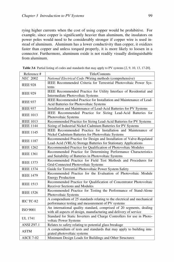
Chapter 3 Introduction to PV Systems 99
rying higher currents when the cost of using copper would be prohibitive. Forexample, since copper is significantly heavier than aluminum, the insulators onpower poles would need to be considerably stronger if copper wire is used in-stead of aluminum. Aluminum has a lower conductivity than copper, it oxidizesfaster than copper and unless torqued properly, it is more likely to loosen in aconnector. Furthermore, aluminum oxide is not readily visually distinguishablefrom aluminum.
Table 3.6 Partial listing of codes and standards that may apply to PV systems [2, 9, 10, 13, 17–20].
Reference # Title/ContentsNEC 2002 National Electrical Code /Wiring methods (comprehensive)
IEEE 928IEEE Recommended Criteria for Terrestrial Photovoltaic Power Sys-tems
IEEE 929IEEE Recommended Practice for Utility Interface of Residential andIntermediate Photovoltaic Systems
IEEE 937IEEE Recommended Practice for Installation and Maintenance of Lead-Acid Batteries for Photovoltaic Systems
IEEE 937 Installation and Maintenance of Lead-Acid Batteries for PV Systems
IEEE 1013IEEE Recommended Practice for Sizing Lead-Acid Batteries forPhotovoltaic Systems
IEEE 1013 Recommended Practice for Sizing Lead-Acid Batteries for PV SystemsIEEE 1144 Sizing of Industrial Nickel Cadmium Batteries for PV Systems
IEEE 1145IEEE Recommended Practice for Installation and Maintenance ofNickel Cadmium Batteries for Photovoltaic Systems
IEEE 1187Recommended Practice for Design and Installation of Valve-RegulatedLead-Acid (VRLA) Storage Batteries for Stationary Applications
IEEE 1262 Recommended Practice for Qualification of Photovoltaic Modules
IEEE 1361Recommended Practice for Determining Performance Characteristicsand Suitability of Batteries in Photovoltaic Systems
IEEE 1373Recommended Practice for Field Test Methods and Procedures forGrid-Connected Photovoltaic Systems
IEEE 1374 Guide for Terrestrial Photovoltaic Power System Safety
IEEE 1479Recommended Practice for the Evaluation of Photovoltaic ModuleEnergy Production
IEEE 1513Recommended Practice for Qualification of Concentrator PhotovoltaicReceiver Sections and Modules
IEEE 1526Recommended Practice for Testing the Performance of Stand-AlonePhotovoltaic Systems
IEC TC-82A compendium of 25 standards relating to the electrical and mechanicalperformance testing and measurement of PV systems
ISO 9001An international quality standard, comprised of 20 segments, dealingwith all aspects of design, manufacturing and delivery of service
UL 1741Standard for Static Inverters and Charge Controllers for use in Photo-voltaic Power Systems
ANSI Z97.1 Relates to safety relating to potential glass breakage
ASTMA compendium of tests and standards that may apply to building inte-grated photovoltaic systems
ASCE 7-02 Minimum Design Loads for Buildings and Other Structures
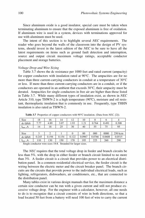
Photovoltaic Systems Engineering100
Since aluminum oxide is a good insulator, special care must be taken whenterminating aluminum to ensure that the exposed aluminum is free of oxidation.If aluminum wire is used in a system, devices with terminations approved foruse with aluminum must be used.
The intent of this section is to highlight several NEC requirements. Thereader who goes beyond the walls of the classroom into the design of PV sys-tems, should invest in the latest edition of the NEC to be sure to have all thelatest requirements on items such as ground fault detection and interruption,source and output circuit maximum voltage ratings, acceptable conductorplacement and storage batteries.
Voltage Drop and Wire SizingTable 3.7 shows the dc resistance per 1000 feet and rated current (ampacity)
for copper conductors with insulation rated at 90°C. The ampacities are for nomore than three current-carrying conductors in conduit at a temperature of 30°Cor less. If more than three current-carrying conductors are in a conduit, or if theconductors are operated in an ambient that exceeds 30°C, their ampacity must bederated. Ampacities for single conductors in free air are higher than those listedin Table 3.7. While many different types of insulation exist, as shown in NECArticle 310, type THWN-2 is a high temperature (90oC), moisture and oil resis-tant, thermoplastic insulation that is commonly in use. Frequently, type THHNinsulation is also rated as THWN-2.
Table 3.7 Properties of copper conductors with 90°C insulation. (Data from NEC, [2]).
Size 18 16 14 12 10 8 6 4dc Ω /kft 7.77 4.89 3.07 1.93 1.21 0.764 0.491 0.308Imax ,A 14 18 25 30 40 55 75 95
Size 3 2 1 0 00 000 0000 250 kcmdc Ω /kft 0.245 0.194 0.154 0.122 0.0967 0.0766 0.0608 0.0515Imax ,A 110 130 150 170 195 225 260 290
Single conductor wire sizes 18–8. Stranded for larger sizes.
The NEC requires that the total voltage drop in feeder and branch circuits beless than 5%, with the drop in either feeder or branch circuit limited to no morethan 3%. A feeder circuit is a circuit that provides power to an electrical distri-bution panel. In a common residential electrical service, the feeder circuit is thewiring between the electric meter and the circuit breaker panel. The branch cir-cuits are the circuits that provide power to the individual electrical loads, such aslighting, refrigerators, dishwashers, air conditioners, etc., that are connected tothe distribution panel.
Many tables exist in various design manuals that list the maximum distance acertain size conductor can be run with a given current and still not produce ex-cessive voltage drop. For the engineer with a calculator, however, all one needsto do is to recognize that a circuit consists of wire in both directions, so that aload located 50 feet from a battery will need 100 feet of wire to carry the current
Chapter 3 Introduction to PV Systems 101
to and from the load. If d is the distance from source to load and Vs is thesource voltage, the percent voltage drop in the wire is thus given by
Ω=
Ω=
kftVId2.0
1000d2
kftVI
100VD%ss
. (3.15)
Example 3.10.1: A 20-watt, 12-VDC fluorescent lamp is located 50 feet from a12 V battery. Specify the wire size needed to keep the voltage drop betweenbattery and lamp under 2%.
Solution. First solve equation (3.15) for ( Ω /kft) to obtain
Id2.0
V)VD(%kft/ s=Ω .
Then, determine the load current from P = IV, assuming the load voltage to beessentially equal to the supply voltage. Substituting the known values on theright hand side yields Ω /kft = (2 × 12)/(0.2 × 1.67 × 50) = 1.437. Table 3.7 showsthat #12 wire has too much resistance, so it is necessary to use #10. The actualvoltage drop with #10 wire can now be found from (3.15) to be 1.68%.
Note that although #10 wire will carry 40 amperes, the current in the circuitis limited to 1.67 amperes due to the voltage drop problem. It is very importantto be aware of the need for larger wire in low voltage systems. Equation (3.15)and Table 3.7 will find considerable use in examples to follow in later chapters.
Because of the problem with voltage drop at low voltages, and the corre-spondingly larger wire sizes necessary, it is generally desirable to operate PVsystems that deliver any significant amounts of power over any reasonable dis-tances at voltages higher than 12 volts. If the previous 20-watt load were con-nected to a 24-volt system, the load current would be halved, and the load volt-age would be doubled. This allows the resistance of the wiring to be four timeshigher, or as much as 5.648 Ω /kft, which means that #16 wire is now adequate.From a total cost standpoint, however, the cost of the additional 12-V batterywill exceed the difference in cost between #10 wire and #16 wire. Presumablythe cost of the PV modules will be the same, since the amount of power requiredhas not changed.
For concealed wiring, the minimum wire size is #14. Smaller wire sizes arenormally used only for portable cords or for attaching single loads.
Switches, Circuit Breakers, Fuses and ReceptaclesAll switches, circuit breakers and fuses used in the dc sections of PV systems
must be rated for use with dc. Switches, circuit breakers and fuses used in accircuits must be rated for ac use. Switches have both current and voltage rat-ings. If a switch is used to control a motor, it must be rated to handle the horse-power of the motor at the operating voltage of the motor.
Photovoltaic Systems Engineering102
Circuit breakers must be sized in accordance with NEC requirements. Al-though the maximum current ratings for #14, #12 and #10 THHN wire are 25,30 and 40 amperes, respectively, the maximum fuse or circuit breaker sizes al-lowed for use with these wire sizes are 15, 20 and 30 amperes, respectively.Larger wire sizes may be fused at their rated ampacities (i.e., Imax).
For motors, it may be necessary to install a fuse or a circuit breaker with arating that exceeds the circuit ampacity in order to accomodate the starting cur-rent of a motor. When this is the case, the motor must have a form of overloadprotection that will disconnect the motor if the motor current exceeds approxi-mately 125% of its rated running current, depending on the size and type ofmotor. Details of wiring for motors and motor controllers are covered in greatdetail in NEC Article 430.
Different voltages require different receptacles. While it is not very likelythat 12 VDC will damage a piece of 120 VAC equipment, except possibly amotor or transformer, it is almost certainly true that 120 VAC will damage apiece of 12 VDC equipment. It is thus necessary to use different attachment capand receptacle configurations for different voltages.
Since the NEC will be referenced in nearly all the design examples in Chap-ters 4, 7 and 8, specific applications of NEC requirements will become moreclearly evident as the examples are developed. Further discussion of overcur-rent protection, disconnects and wire sizing in accordance with NEC require-ments will be covered in detail in these examples.
Ground Fault, Surge and Lightning ProtectionPresumably, current will leave the PV array via the positive conductor and
the same amount of current will return to the array via the negative conductor.This will be the case, provided that no alternate return paths are present.
The NEC requires that metallic frames and other metal parts of PV systemsbe connected to ground. The conductors used for this purpose are calledgrounding conductors. Generally, the negative conductor is also connected toground at some point along the system. If so, then the negative conductor iscalled the grounded conductor. Since the negative conductor is connected toground at only one point, current will flow in the grounded conductor, but willnot flow in any of the grounding conductors, since there is no closed circuit inwhich the current can flow.
However, if for some reason the positive conductor were connected toground, then there would be an alternate closed path in which current would beable to flow through the grounding conductors. If this is the case, thenKirchhoff’s current law requires that the current in the positive conductor willequal the sum of the currents in the grounded and grounding conductors. Thenet result is that no longer will the currents in the positive and negative(grounded) conductors be equal. The greatest danger in dc ground fault currentsin a PV system is the means by which they are established. If the ground faultresults from a loose connection, the connection may begin to arc and become afire hazard.

Chapter 3 Introduction to PV Systems 103
The NEC requires that if an array is rooftop mounted on a dwelling, thenground fault protection must be provided to disconnect the array in the event ofa difference in current between the positive and negative array conductors lead-ing to the controller/inverter/loads.
Another important component used to provide protection to the array andinverter is the surge protector. Surge protectors are similar to zener diodes inthat they are made of material that is essentially insulating until a predeterminedvoltage appears across the material. At this point, avalanche breakdown occursand the surge protector acts as a current shunt. Metal oxide varistor (MOV)types of surge protector respond in nanoseconds and can bypass many joules ofsurge energy. However, a disadvantage of MOV surge protectors is that theydraw a small current at all times and generally the failure mode of a MOV de-vice is a short circuit. SiO (SOV) surge protectors are an improvement in termsof the MOV disadvantages. It is good practice to incorporate surge protectioninto system design at a location close to the common system ground point.
Additional protection from lightning strikes can be obtained with lightningrod systems. Contrary to popular belief, lightning rods do not attract lightning.Rather, they present a sharp point (or points) that are connected to ground. If apotential difference should appear between the rod and the surrounding atmos-phere, a very high electric field builds up around the point to the extent that acorona discharge takes place, equalizing the charge between the air and theground. Corona discharge is also known as glow discharge. Lightning is knownas arc discharge. Arc discharge is violent, but glow discharge is essentiallyharmless since the charge is equalized over a much longer period of time.
3.10.3 IEEE Standard 929-2000
IEEE 929-2000 deals with the utility interface of grid-connected systems. Itaddresses concerns of utilities regarding quality of power delivered to the gridand the need to disconnect the PV system from the utility grid in the event ofutility power failure. IEEE 929-2000, while specific to grid-connected PV sys-tems, incorporates the general requirements of several other standards, includingUL 1741 on the testing of grid-connected inverters, IEEE 519-1992 on harmoniccontrol and ANSI C84.1–1995 on voltage and voltage ratings in 6 0 Hz systems.
IEEE 929-2000 establishes standards relating to voltage disturbances, fre-quency disturbances, islanding protection, power factor, reconnect after gridfailure and restoration, injection of dc into an ac system, grounding, surge pro-tection and dc and ac disconnects.
Voltage at the inverter output, for example, should not be more than 5%higher than the voltage at the point of utility connection. The inverter should beable to sense grid voltage abnormalities and shut down the inverter when indi-cated. Shutdown should occur within 6 cycles if the utility voltage, V, dropsbelow 50% of its nominal value. If 50% < V < 88% or if 110% < V < 137% ofnominal, then the inverter must shut down within 120 cycles. For V > 137% ofnominal, shutdown must occur within 2 cycles. If the line frequency falls below
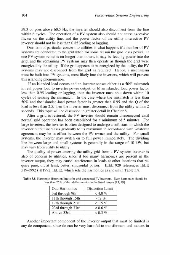
Photovoltaic Systems Engineering104
59.3 or goes above 60.5 Hz, the inverter should also disconnect from the linewithin 6 cycles. The operation of a PV system also should not cause excessiveflicker on the utility line, and the power factor of the utility interactive PVinverter should not be less than 0.85 leading or lagging.
One item of particular concern to utilities is what happens if a number of PVsystems are connected to the grid when for some reason the grid loses power. Ifone PV system remains on longer than others, it may be feeding power into thegrid, and the remaining PV systems may then operate as though the grid wereenergized by the utility. If the grid appears to be energized by the utility, the PVsystems may not disconnect from the grid as required. Hence, a mechanismmust be built into PV systems, most likely into the inverters, which will preventthis islanding phenomenon.
If an islanded load occurs and an inverter senses either a) a 50% mismatchin real power load to inverter power output, or b) an islanded load power factorless than 0.95 leading or lagging, then the inverter must shut down within 10cycles of sensing the mismatch. In the case where the mismatch is less than50% and the islanded-load power factor is greater than 0.95 and the Q of theload is less than 2.5, then the inverter must disconnect from the utility within 2seconds. This topic will be discussed in greater detail in Chapter 8.
After a grid is restored, the PV inverter should remain disconnected untilnormal grid operation has been established for a minimum of 5 minutes. Forlarge inverters, the inverter is often designed to undergo a soft start, in which theinverter output increases gradually to its maximum in accordance with whateveragreement may be in effect between the PV owner and the utility. For smallsystems, the inverter may switch on to full power immediately. The dividingline between large and small systems is generally in the range of 10 kW, butmay vary from utility to utility.
The quality of power entering the utility grid from a PV system inverter isalso of concern to utilities, since if too many harmonics are present in theinverter output, they may cause interference in loads at other locations that re-quire pure, or, at least, better, sinusoidal power. IEEE 929 references IEEE519–1992 ( 1992, IEEE), which sets the harmonics as shown in Table 3.8.
Table 3.8 Harmonic distortion limits for grid-connected PV inverters. Even harmonics should beless than 25% of the odd harmonics in the listed ranges [13, 19].
Odd Harmonics Distortion Limit3rd through 9th < 4.0 %11th through 15th < 2 %17th through 21st < 1.5 %23rd through 33rd < 0.6 %Above 33rd < 0.3 %
Another important component of the inverter output that must be limited isany dc component, since dc can be very harmful to transformers and motors in
Chapter 3 Introduction to PV Systems 105
an ac system. Inverter dc output current must be no greater than 0.5% of ratedinverter output current.
Discussions of optimal protection from islanding and allowable inverter out-put harmonic levels are ongoing. Inverters that supply utility interactive loadsare of particular interest, especially those that provide for battery backup of gridpower. Until more field data is available, the discussions will continue, basedon limited theoretical studies and limited testing. Perhaps the reader of this textwill one day also contribute to the discussion if he or she is not already doing so.
3.11 Balance of System Components
The balance of system (BOS) components include mounting materials forthe modules, wire and all wiring components, lightning protectors, groundingconnections and battery containers. In some cases, the connected loads are con-sidered to be part of the BOS and in other cases the loads are not considered tobe a part of the system. The distinction is generally made when the system isinstalled to operate a specific load, as opposed to being installed to be one con-tributor to the operation of any load.
Certain BOS components are regulated by codes or standards. Arraymounts, for example, must meet any windloading requirements of applicablebuilding codes. Battery compartments are covered in the NEC.
In certain environments, BOS components may need to be resistant to corro-sion from exposure to salt air or may need to be appropriate for other environ-mental considerations. If a PV system is part of a building integrated structure,then a number of other codes and standards may become applicable.
Problems
3.1 If I = 2 A, Io = 10–10 A and T = 300 K for a PV cell, determine the maxi-mum power point of the cell by differentiating the expression obtained bymultiplying Equation (3.1) by the cell voltage.
3.2 Determine the range of operating voltages for which a 36-cell module willhave power output within 90% of maximum power. You may assume Io =10–10 A and VOC = 0.596 V at an operating temperature of 300 K. Assumeall cells in the module to be identical.
3.3 A PV module is found to operate at a temperature of 60oC under conditionsof TA = 30oC and G = 980 W/m2. Determine the NOCT of the module.
3.4 Plot Vm vs. T for –25 < T < +75 oC for a 36-cell Si module for which eachcell has Vm = 0.5 V at 25oC.
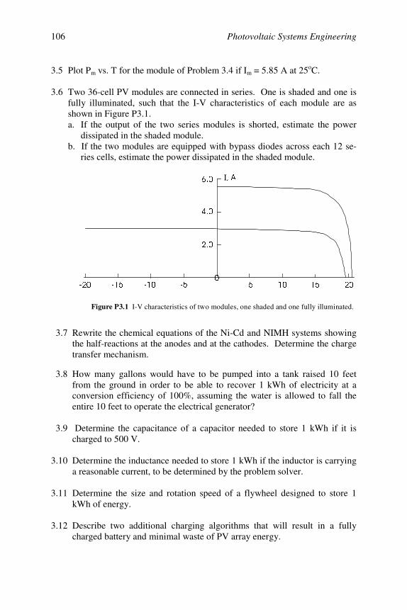
Photovoltaic Systems Engineering106
3.5 Plot Pm vs. T for the module of Problem 3.4 if Im = 5.85 A at 25oC.
3.6 Two 36-cell PV modules are connected in series. One is shaded and one isfully illuminated, such that the I-V characteristics of each module are asshown in Figure P3.1.a. If the output of the two series modules is shorted, estimate the power
dissipated in the shaded module.b. If the two modules are equipped with bypass diodes across each 12 se-
ries cells, estimate the power dissipated in the shaded module.
3.7 Rewrite the chemical equations of the Ni-Cd and NIMH systems showingthe half-reactions at the anodes and at the cathodes. Determine the chargetransfer mechanism.
3.8 How many gallons would have to be pumped into a tank raised 10 feetfrom the ground in order to be able to recover 1 kWh of electricity at aconversion efficiency of 100%, assuming the water is allowed to fall theentire 10 feet to operate the electrical generator?
3.9 Determine the capacitance of a capacitor needed to store 1 kWh if it ischarged to 500 V.
3.10 Determine the inductance needed to store 1 kWh if the inductor is carryinga reasonable current, to be determined by the problem solver.
3.11 Determine the size and rotation speed of a flywheel designed to store 1kWh of energy.
3.12 Describe two additional charging algorithms that will result in a fullycharged battery and minimal waste of PV array energy.
I$
Figure P3.1 I-V characteristics of two modules, one shaded and one fully illuminated.
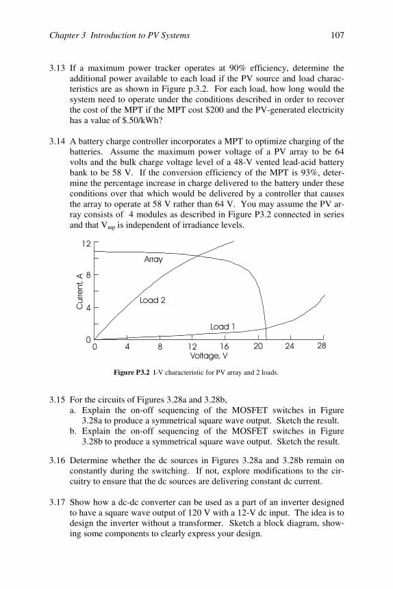
Chapter 3 Introduction to PV Systems 107
3.13 If a maximum power tracker operates at 90% efficiency, determine theadditional power available to each load if the PV source and load charac-teristics are as shown in Figure p.3.2. For each load, how long would thesystem need to operate under the conditions described in order to recoverthe cost of the MPT if the MPT cost $200 and the PV-generated electricityhas a value of $.50/kWh?
3.14 A battery charge controller incorporates a MPT to optimize charging of thebatteries. Assume the maximum power voltage of a PV array to be 64volts and the bulk charge voltage level of a 48-V vented lead-acid batterybank to be 58 V. If the conversion efficiency of the MPT is 93%, deter-mine the percentage increase in charge delivered to the battery under theseconditions over that which would be delivered by a controller that causesthe array to operate at 58 V rather than 64 V. You may assume the PV ar-ray consists of 4 modules as described in Figure P3.2 connected in seriesand that Vmp is independent of irradiance levels.
3.15 For the circuits of Figures 3.28a and 3.28b,a. Explain the on-off sequencing of the MOSFET switches in Figure
3.28a to produce a symmetrical square wave output. Sketch the result.b. Explain the on-off sequencing of the MOSFET switches in Figure
3.28b to produce a symmetrical square wave output. Sketch the result.
3.16 Determine whether the dc sources in Figures 3.28a and 3.28b remain onconstantly during the switching. If not, explore modifications to the cir-cuitry to ensure that the dc sources are delivering constant dc current.
3.17 Show how a dc-dc converter can be used as a part of an inverter designedto have a square wave output of 120 V with a 12-V dc input. The idea is todesign the inverter without a transformer. Sketch a block diagram, show-ing some components to clearly express your design.
Figure P3.2 I-V characteristic for PV array and 2 loads.
Photovoltaic Systems Engineering108
3.18 For the 5-level H-Bridge of Figure 3.31, determine T2 if T1 = T0, Vrms =120 V, anda. Vdc = 150 Vb. Vdc = 155 Vc. Vdc = 160 Vd. Vdc = 165 VNote that Excel or MATLAB can be very useful for this problem.
3.19 For the 5-level H-Bridge of Figure 3.31, determine a set of values of T0, T1
and T2 that will minimize the total harmonic distortion of the waveform ifVdc = 160 V and Vrms = 120 V. A convenient tool is to construct the wave-form in PSPICE using series pulse voltage sources and then to run a FastFourier Transform of the resulting waveform.
3.20 For the 5-level H-Bridge of Figure 3.31, determine the maximum value forVdc if the design requires T2 > 0.025T and T0 > 0.025T.
3.21 Referring to Figure 3.31a, design a 7-level H-Bridge, using 4 capacitorsand an appropriate number of series switches in each string. Show thewaveform and the switching needed to obtain each of the 7 levels of theoutput voltage.
3.22 For the 7-level H-Bridge output waveform, derive a formula for the rmsvalue of the output voltage.
3.23 Construct the 7-level H-Bridge output waveform using series pulse voltagesources in PSPICE and perform a Fast Fourier Transform on the waveformto explore the harmonic distortion of the waveform. Keep Vdc and Vrms
constant, while varying the duration of the different levels of the waveformin order to minimize the total harmonic distortion (THD) of the waveform.
3.24 Make a list of loads that might confuse an inverter that is in the “sleep”mode. Explain why each load causes a problem.
3.25 The following data are given for a series of gasoline-powered electricalgenerators:
Rated output 1500 W 2300 W 3000 W 4500 WFuel tank size 2.9 gal 2.9 gal 4.5 gal 4.5 gal
Run time/ tankful 9 hr 9 hr 8.3 hr 5.6 hr
Calculate the kWh/gal for each of these generators under rated load condi-tions.
Chapter 3 Introduction to PV Systems 109
3.26 Refer to Table 3.7 or to the NEC in order to:a. Determine the wire size needed to limit voltage drop to 3% for a 100-
watt, 24-volt load at a distance of 75 feet from the voltage source.b. Using the wire size determined in part a, determine the actual voltage
drop for the wiring.
References
[1] Maintenance and Operation of Stand-Alone Photovoltaic Systems, Sandia NationalLaboratories, Albuquerque, NM, 1991.
[2] NFPA 70 National Electrical Code , 2002 Ed., National Fire Protection Association,Quincy, MA, 2002. [1] Markvart, T., Ed., Solar Electricity, John Wiley & Sons,Chichester, U.K., 1994.
[3] IEEE Standard 1187-2002, IEEE Recommended Practice for Installation Designand Installation of Valve-Regulated Lead-Acid Storage Batteries for Stationary Ap-plications, Institute of Electrical and Electronics Engineers, Inc., New York, 2002.
[4] Linden, D., Ed., Handbook of Batteries, 2nd Ed., McGraw-Hill, New York, 1994. [5] Hancock, Jr., O. G., Hydrogen storage: the hydrogen alternative, Photovoltaics In-
ternational, March, 1986. [6] Skerrett, P. J., Fuel UPD, Pop. Science, June, 1993. [7] Roland, B., Nitsch, J. and Wendt, H., Hydrogen and Fuel Cells-the Clean Energy
System, Elsevier Sequoia, Oxford, U.K., 1992. [8] Stand-Alone Photovoltaic Systems: A Handbook of Recommended Design Practices,
Sandia National Laboratories, Albuquerque, NM, 1995. [9] UL 1741: 1999, Standard for Static Inverters and Charge Controllers for Use in
Photovoltaic Power Systems, Underwriters Laboratories, Inc., Northbrook, IL, May1999.
[10] ANSI C84.1–1995, Electric Power Systems and Equipment – Vol tage Ratings (60Hertz), American National Standards Institute, New York, 1995.
[11] http://www.xantrex.com/ (Information on Trace/Xantrex Power Electronics Equip-ment.)
[12] http://www.omnion.com/ (Information on Omnion Power Electronics Equipment.)[13] IEEE 929-2000, IEEE Recommended Practice for Utility Interface of Residential
and Intermediate Photovoltaic (PV) Systems, IEEE Standards Coordinating Com-mittee 21, Photovoltaics, 2000.
[14] Trace Engineering Company, Inc., “SW Series Inverter/Charge rs With Revision4.01 Software Owner’s Manual,” Arlington, WA, September 1999.
[15] http://www.mayberrys.com/ (Additional information on Honda generators from DonMayberry, Jr., Mayberry Sales and Service, Inc., Port Murray, NJ).
[16] Onan Corporation, Minneapolis, MN, sales literature on Onan generators, including“Gensize ‘96” software for sizing generator sets.

Photovoltaic Systems Engineering110
[17] Wohlgemuth, J., “Testing for BIPV,” Proc. Photovoltaic Performance and Reliabil-ity Workshop, Cocoa Beach, FL, November 1998, 113.
[18] DeBlasio, R., “Status of IEEE Standards Coordinating Commit tee (SCC 21) andIEC Standards Technical Committee 82 (TC82),” Proc. Photovoltaic Performanceand Reliability Workshop, Cocoa Beach, FL, November 1998, 236.
[19] IEEE Standard 519–1992, Recommended Practices and Requirements for HarmonicControl in Electrical Power Systems, Institute of Electrical and Electronics Engi-neers, Inc., New York, 1992.
[20] Zgonena, T., “Safety Considerations for Static Grid-Tied Ph otovoltaic Inverters,”Interconnecting Small PV Systems to Florida’s Utility Grid, A Technical Workshopfor Florida’s Utilities, Cocoa, FL, October 22, 1998.
[21] Danley, D. R., Orion Energy Corporation, Ijamsville, MD, Personal communicationregarding fuel efficiency of fossil-fueled generators, August, 1999.
Suggested Reading
ASCE Standard 7-02, Minimum Design Loads for Buildings and Other Structures,American Society of Civil Engineers, Reston, VA, 2000.
Hoogers, G., Ed., Fuel Cell Technology Handbook, CRC Press, Boca Raton, FL,2002.
Hu, C. and White, R., Solar Cells: From Basics to Advanced Systems, McGraw-Hill,New York, 1983.
Krein, Philip T., Elements of Power Electronics, Oxford University Press, NewYork, 1998.
Roden, M. S. and Carpenter, G. L., Electronic Design: From Concept to Reality,Discovery Press, Burbank, CA, 1997.
Sedra, A. S. and Smith, K. C., Microelectronic Circuits, 4th Ed., Oxford UniversityPress, New York, 1998.
Silberberg, M., Chemistry: The Molecular Nature of Matter and Change, Mosby, St.Louis, 1996.
Skvarenina, T. L., ed, The Power Electronics Handbook, CRC Press, Boca Raton,FL, 2002.
Vithayathil, J., Power Electronics: Principles and Applications, McGraw-Hill, NewYork, 1995.
111
Chapter 4PV SYSTEM EXAMPLES
4.1 Introduction
Analysis is the next stop on the road to design. In this chapter, several PVsystems will be analyzed in order to acquaint the reader with some of the consid-erations used in the design of systems. Analysis of the systems should encour-age the reader to think of alternative means of achieving the desired end result,since normally there is no single best solution to a design problem. If therewere, the world would be a boring place, with only one model of automobile,one model of computer, one model of television, and, perhaps worst of all, eve-ryone would be wearing the same uniform. The engineer can thus be grateful fordiversity in the world.
In each example, an effort will be made to point out the areas where the PVsystem is open to the discretion of the designer. Perhaps reliability, performanceand cost are among the items of most common concern. It is often the case thatthere will be a trade-off among these three parameters. Chapter 5 has been in-cluded to provide the designer with quantitative means of dealing with cost con-siderations. Other considerations commonly overlooked include environmentalimpact, safety and aesthetics. These topics are discussed in greater detail withregard to energy systems in Chapter 9.
The first few examples in this chapter are relatively simple systems. In eachcase, the systems could be made more complicated to increase performance, butit should be remembered that complexity often results in a sacrifice in reliability,and almost certainly involves an increase in price. Simplicity, thus, should beacknowledged as having an elegance of its own, and should not necessarily bediscarded as an option.
The final examples are more complex, and are intended to demonstrate thewide range of applications of PV power systems. In these examples, it will be-come evident that there are many options and tradeoffs involved in reaching thefinal system design.
4.2 Example 1: A Simple PV-Powered Fan
4.2.1 The Simplest Configuration: Module and Fan
Figure 4.1 shows the simplest of PV systems, a fan motor connected to a PVmodule. The figure also shows the superimposed performance (I-V) character-istics of the fan and the module. The operation is simple: as the sun shinesbrighter, the fan turns faster. If the designer has no concern for the exact quan-tity of air moved, the design becomes nearly trivial. However, if the amount ofair moved must meet a code requirement or other constraint, then it will be nec-essary to consider the design in more detail.
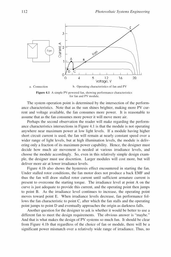
Photovoltaic Systems Engineering112
The system operation point is determined by the intersection of the perform-ance characteristics. Note that as the sun shines brighter, making more PV cur-rent and voltage available, the fan consumes more power. It is reasonable toassume that as the fan consumes more power it will move more air.
Perhaps the second observation the reader will make regarding the perform-ance characteristics intersections in Figure 4.1 is that the module is not operatinganywhere near maximum power at low light levels. If a module having highershort circuit current is used, the fan will remain at nearly constant speed over awider range of light levels, but at high illumination levels, the module is deliv-ering only a fraction of its maximum power capability. Hence, the designer mustdecide how much air movement is needed at various irradiance levels, andchoose the module accordingly. So, even in this relatively simple design exam-ple, the designer must use discretion. Larger modules will cost more, but willdeliver more air at lower irradiance levels.
Figure 4.1b also shows the hysteresis effect encountered in starting the fan.Under stalled rotor conditions, the fan motor does not produce a back EMF andthus the fan will draw stalled rotor current until sufficient armature current ispresent to overcome the starting torque. The irradiance level at point A on thecurve is just adequate to provide this current, and the operating point then jumpsto point B. As the irradiance level continues to increase, the operating pointmoves toward point E. When irradiance levels decrease, fan performance fol-lows the fan characteristic to point C, after which the fan stalls and the operatingpoint jumps to point D and eventually approaches the origin as darkness falls.
Another question for the designer to ask is whether it would be better to use adifferent fan to meet the design requirements. The obvious answer is “maybe.”And that is what makes the design of PV systems so much fun. It should be clearfrom Figure 4.1b that regardless of the choice of fan or module, there will be asignificant power mismatch over a relatively wide range of irradiance. Thus, no
a. Connection b. Operating characteristics of fan and PV
Figure 4.1 A simple PV-powered fan, showing performance characteristics for fan and PV module.
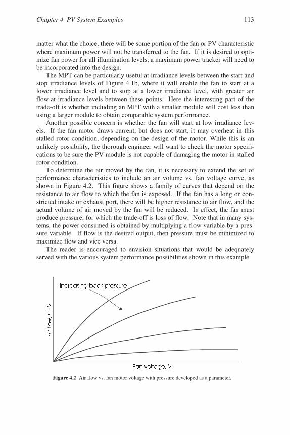
Chapter 4 PV System Examples 113
matter what the choice, there will be some portion of the fan or PV characteristicwhere maximum power will not be transferred to the fan. If it is desired to opti-mize fan power for all illumination levels, a maximum power tracker will need tobe incorporated into the design.
The MPT can be particularly useful at irradiance levels between the start andstop irradiance levels of Figure 4.1b, where it will enable the fan to start at alower irradiance level and to stop at a lower irradiance level, with greater airflow at irradiance levels between these points. Here the interesting part of thetrade-off is whether including an MPT with a smaller module will cost less thanusing a larger module to obtain comparable system performance.
Another possible concern is whether the fan will start at low irradiance lev-els. If the fan motor draws current, but does not start, it may overheat in thisstalled rotor condition, depending on the design of the motor. While this is anunlikely possibility, the thorough engineer will want to check the motor specifi-cations to be sure the PV module is not capable of damaging the motor in stalledrotor condition.
To determine the air moved by the fan, it is necessary to extend the set ofperformance characteristics to include an air volume vs. fan voltage curve, asshown in Figure 4.2. This figure shows a family of curves that depend on theresistance to air flow to which the fan is exposed. If the fan has a long or con-stricted intake or exhaust port, there will be higher resistance to air flow, and theactual volume of air moved by the fan will be reduced. In effect, the fan mustproduce pressure, for which the trade-off is loss of flow. Note that in many sys-tems, the power consumed is obtained by multiplying a flow variable by a pres-sure variable. If flow is the desired output, then pressure must be minimized tomaximize flow and vice versa.
The reader is encouraged to envision situations that would be adequatelyserved with the various system performance possibilities shown in this example.
Figure 4.2 Air flow vs. fan motor voltage with pressure developed as a parameter.
Photovoltaic Systems Engineering114
4.2.2 PV Fan with Battery Backup
It is not difficult to imagine a situation where it is desired to use a fan attimes when the sun is not shining. For that matter, it is perhaps even easier toenvision a situation where it is desired to use a light when the sun is not shining.In either case, it will be necessary to store energy for later use. Figure 4.3 showsa PV fan system that includes storage batteries in the system. In this system, it isnecessary to match the fan to the batteries as well as to the module(s). This isdone by first determining the hours of operation of the fan as well as the energyto be used by the fan. Once again, the range of choices may be limitless.
Suppose that it has been determined that the fan must run continuously, and,since the fan will be operating from the battery, the fan voltage will be the bat-tery voltage, which will presumably remain relatively constant. In this case, it isa simple matter to determine the daily energy consumption of the fan, since con-stant fan voltage will produce constant fan power. For example, if the fan motorconsumes 24 watts when run from a nominal 12-volt battery, then in one day thefan will consume (24 watts)×(24 hours) = 576 Wh of electrical energy.
The battery capacity, however, will be measured in ampere-hours (Ah). Todetermine the connected load in Ah for the fan, simply divide the energy by thevoltage. In this case, the result is 48 Ah. Note that this result is also determinedby multiplying the load current by the run time, or, if the load current is not con-stant, then the load current must be integrated over the time of operation.
Since neither the battery charging and discharging nor the wiring are 100%efficient, it is not adequate to consider only the connected load Ah requirements.The corrected load is determined by dividing the connected load by the batteryefficiency and by the wiring efficiency. Typically, 90% of the charging energycan be recovered, and wiring losses are about 2%. So the corrected load be-comes 48÷0.9÷0.98 = 54.4 Ah.
Next, it must be determined how critical it is that the fan run all the time. Iffan operation is critical, then sufficient battery storage must be provided topower the fan during long periods of darkness or cloudy weather. The antici-pated duration of such periods will depend on the geographical location of thefan and on whether the use of the fan is seasonal. Suppose this has all beenworked out and that it has been determined that three days of storage is adequate.This means that a total storage capacity of 163 Ah is needed.
At this point, a decision must be made as to what type of battery to use.Suppose a lead-antimony storage battery is chosen. Since the lead-antimonysystem will allow deep discharge, suppose the battery (or batteries) is allowed todischarge to 20% of full charge. This means that only 80% of the battery ratingis available for use. The capacity needed for this design is thus 163÷0.8 = 204Ah. This capacity might be obtained with a single 12-volt, 204 Ah battery, butmore likely would be obtained with two 6-volt batteries connected in series,since a 12-volt, 204 Ah lead-acid battery would be heavy and difficult to handle.Smaller units will usually be a more practical choice, as long as no more than 4
Chapter 4 PV System Examples 115
sets of batteries need to be connected in parallel. If more than 4 sets of batteriesare connected in parallel, the chance of unbalance in battery charging and dis-charging currents is increased. This can cause premature battery failure.
Next, it is necessary to specify the PV power needs. This is done by deter-mining the times when the least amount of sunlight is available during themonths in which the fan is to operate. Suppose this has been done and it hasbeen determined that the equivalent of 4 hours of full sun is available in theworst case. This does not imply that the sun shines at maximum intensity for 4hours and then sets beyond the horizon, but that the average intensity over day-light hours is the same as peak intensity for 4 hours. It means that on some days,more than 4 hours of peak sun will be available and on some days, less than 4hours of peak sun will be available.
During this 4-hour period, the PV array must produce all the electricityneeded to operate the fan for a day. If a PV array with a nominal 12 V output isused, then the array must produce the needs of the batteries in ampere hours.However, it must be taken into account that the PV modules may not alwaysoperate at peak efficiency, such as if they get dusty. Operation at cell tempera-tures higher than 25oC may reduce maximum output power by an additional 15%by reducing the module maximum power voltage by 15%. Thus, rather thandesigning the PV system to produce the daily corrected load of 54.4 Ah, thesystem should be designed to produce 54.4÷0.9 = 60.4 Ah. This amount allowsfor a 10% degradation of PV module output and assumes the module will thenproduce the necessary charging current at the charging voltage of the batteries,which is normally approximately 15 volts.
Since the available full sun is 4 hours, this means the PV module output mustbe (60.4 Ah)÷(4 hr) = 15.1 A. So, finally, assuming the use of modules capableof producing 5.04 A at 15 V, a total of 3 modules will need to be connected inparallel to produce the necessary 15.1 A.
The design of the system is now nearly complete. In the event that the sun ishidden for more than 3 days, the batteries may discharge below the 20% level.Secondly, during the months of the year when more than 4 peak sun hours areavailable, the batteries may overcharge. These situations are mitigated some-what by the fact that the fan motor runs faster and consumes more energy whenthe battery voltage is higher and conversely runs more slowly and consumes lessenergy when the battery voltage is lower. Yet, both situations can result in short-ening of the life of the batteries. So good design practice would include a chargecontroller to prevent overcharge or overdischarge of the batteries. The chargecontroller must be capable of handling at least 125% of the total PV short-circuitoutput current on a continuous basis. It must also handle the fan current on acontinuous basis.
Additional BOS components may also be considered, such as lightning surgeprotectors. More details on these items will follow in Chapter 7. Figure 4.3shows the fan system with batteries and charge controller.
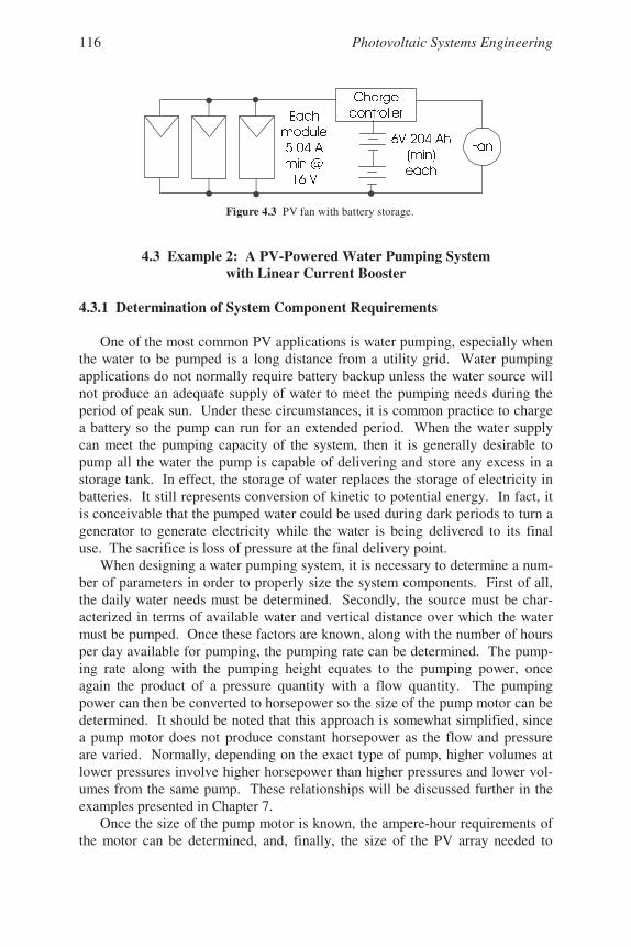
Photovoltaic Systems Engineering116
4.3 Example 2: A PV-Powered Water Pumping Systemwith Linear Current Booster
4.3.1 Determination of System Component Requirements
One of the most common PV applications is water pumping, especially whenthe water to be pumped is a long distance from a utility grid. Water pumpingapplications do not normally require battery backup unless the water source willnot produce an adequate supply of water to meet the pumping needs during theperiod of peak sun. Under these circumstances, it is common practice to chargea battery so the pump can run for an extended period. When the water supplycan meet the pumping capacity of the system, then it is generally desirable topump all the water the pump is capable of delivering and store any excess in astorage tank. In effect, the storage of water replaces the storage of electricity inbatteries. It still represents conversion of kinetic to potential energy. In fact, itis conceivable that the pumped water could be used during dark periods to turn agenerator to generate electricity while the water is being delivered to its finaluse. The sacrifice is loss of pressure at the final delivery point.
When designing a water pumping system, it is necessary to determine a num-ber of parameters in order to properly size the system components. First of all,the daily water needs must be determined. Secondly, the source must be char-acterized in terms of available water and vertical distance over which the watermust be pumped. Once these factors are known, along with the number of hoursper day available for pumping, the pumping rate can be determined. The pump-ing rate along with the pumping height equates to the pumping power, onceagain the product of a pressure quantity with a flow quantity. The pumpingpower can then be converted to horsepower so the size of the pump motor can bedetermined. It should be noted that this approach is somewhat simplified, sincea pump motor does not produce constant horsepower as the flow and pressureare varied. Normally, depending on the exact type of pump, higher volumes atlower pressures involve higher horsepower than higher pressures and lower vol-umes from the same pump. These relationships will be discussed further in theexamples presented in Chapter 7.
Once the size of the pump motor is known, the ampere-hour requirements ofthe motor can be determined, and, finally, the size of the PV array needed to
Figure 4.3 PV fan with battery storage.
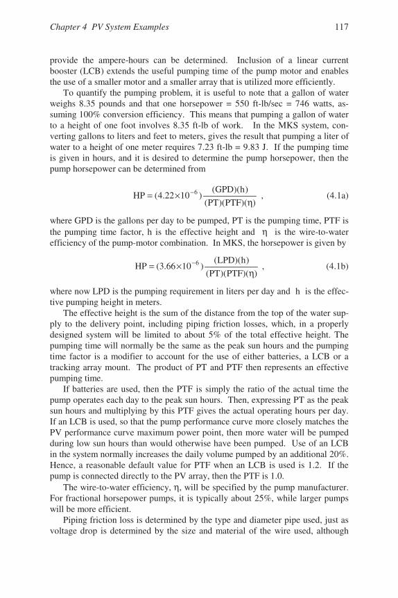
Chapter 4 PV System Examples 117
provide the ampere-hours can be determined. Inclusion of a linear currentbooster (LCB) extends the useful pumping time of the pump motor and enablesthe use of a smaller motor and a smaller array that is utilized more efficiently.
To quantify the pumping problem, it is useful to note that a gallon of waterweighs 8.35 pounds and that one horsepower = 550 ft-lb/sec = 746 watts, as-suming 100% conversion efficiency. This means that pumping a gallon of waterto a height of one foot involves 8.35 ft-lb of work. In the MKS system, con-verting gallons to liters and feet to meters, gives the result that pumping a liter ofwater to a height of one meter requires 7.23 ft-lb = 9.83 J. If the pumping timeis given in hours, and it is desired to determine the pump horsepower, then thepump horsepower can be determined from
))(PTF)(PT(
)h)(GPD()1022.4(HP 6
η×= − , (4.1a)
where GPD is the gallons per day to be pumped, PT is the pumping time, PTF isthe pumping time factor, h is the effective height and η is the wire-to-waterefficiency of the pump-motor combination. In MKS, the horsepower is given by
))(PTF)(PT(
)h)(LPD()1066.3(HP 6
η×= − , (4.1b)
where now LPD is the pumping requirement in liters per day and h is the effec-tive pumping height in meters.
The effective height is the sum of the distance from the top of the water sup-ply to the delivery point, including piping friction losses, which, in a properlydesigned system will be limited to about 5% of the total effective height. Thepumping time will normally be the same as the peak sun hours and the pumpingtime factor is a modifier to account for the use of either batteries, a LCB or atracking array mount. The product of PT and PTF then represents an effectivepumping time.
If batteries are used, then the PTF is simply the ratio of the actual time thepump operates each day to the peak sun hours. Then, expressing PT as the peaksun hours and multiplying by this PTF gives the actual operating hours per day.If an LCB is used, so that the pump performance curve more closely matches thePV performance curve maximum power point, then more water will be pumpedduring low sun hours than would otherwise have been pumped. Use of an LCBin the system normally increases the daily volume pumped by an additional 20%.Hence, a reasonable default value for PTF when an LCB is used is 1.2. If thepump is connected directly to the PV array, then the PTF is 1.0.
The wire-to-water efficiency, η, will be specified by the pump manufacturer.For fractional horsepower pumps, it is typically about 25%, while larger pumpswill be more efficient.
Piping friction loss is determined by the type and diameter pipe used, just asvoltage drop is determined by the size and material of the wire used, although
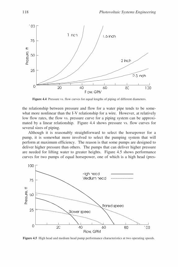
Photovoltaic Systems Engineering118
the relationship between pressure and flow for a water pipe tends to be some-what more nonlinear than the I-V relationship for a wire. However, at relativelylow flow rates, the flow vs. pressure curve for a piping system can be approxi-mated by a linear relationship. Figure 4.4 shows pressure vs. flow curves forseveral sizes of piping.
Although it is reasonably straightforward to select the horsepower for apump, it is somewhat more involved to select the pumping system that willperform at maximum efficiency. The reason is that some pumps are designed todeliver higher pressure than others. The pumps that can deliver higher pressureare needed for lifting water to greater heights. Figure 4.5 shows performancecurves for two pumps of equal horsepower, one of which is a high head (pres-
Figure 4.4 Pressure vs. flow curves for equal lengths of piping of different diameters.
Figure 4.5 High head and medium head pump performance characteristics at two operating speeds.
Chapter 4 PV System Examples 119
sure) pump and the other is a medium head pump.Note that the medium head pump will deliver more volume than the high
head pump at low pressure, but the high head pump will overcome a greaterpumping height. Note also that the performance of a pump depends on the speedat which the pump is operated. If the pump speed decreases, both pressure andflow capacity decrease. It is thus important to select a pump that will be able toovercome the lift requirement under low sun conditions.
4.3.2 A Simple Pumping System
Suppose a volume of 2000 gallons per day is required for irrigation purposes.Suppose also that the reservoir from which the water is to be pumped is verylarge, but located 200 feet underground, and that the worst case peak sun hoursduring the irrigation period is 6 hours. The problem is to determine the neces-sary components for a PV water pumping system to supply this water.
First, from (4.1a), the pump HP can be determined, assuming PTF = 1, peaksun of 6 hours and 25% pump efficiency, along with 5% piping friction losses.Taking the 5% piping losses into account, the effective height becomes1.05×200 = 210 ft. Note that it is assumed that the water is being distributed atground level with no storage. Using this value of h in (4.1a) along with the othersystem variables yields HP = 1.18. Of course, pumps do not come in 1.18 HPsizes, so the system designer now must choose from available sizes, meaningeither a 1 HP or a 1.5 HP pump.
This is where the notion of service factor is useful. Motors are designed withservice factor ratings. The service factor represents the amount of overload towhich a motor may be subjected on a continuous basis without damaging themotor. A service factor of 1.25 for a 1 HP motor is not unusual. Hence, a 1 HPmotor with a service factor of 1.25 can deliver the needed 1.18 HP. It shouldalso be remembered that the pump motor will only be delivering maximum HPfor at most a few hours near solar noon. Prior to and after this period, the pumpwill receive less power from the PV array and will thus operate at a lower HP.
Since the pump is connected directly to the array, the array size can thus bedetermined by installing the same current at full sun as the pump requirement,taking into account a 10% PV array degradation factor. Using a 10% degrada-tion factor, the array current would be (1.18 HP)×(746 watts/HP)×(1.1)÷(24 V)= 40.3 A, assuming a 24 V pump motor. Note that the motor efficiency has al-ready been accounted for in the overall wire-to-water efficiency estimate, so nofurther increase in array current is required for the pump motor.
Assuming 7 A at peak sun modules, a total of 12 modules will be needed tosupply 42 A at a nominal voltage of 24 V, which should be close enough to thedesign requirement. If an LCB is used, then the PTF will be 1.2, and the newrequired HP is 20% less, since the pump operates 20% more efficiently. Thiswill require only 0.8×42 = 35 A, which will require 10 modules. The questionthen is whether the price of the two additional modules is greater than the cost of
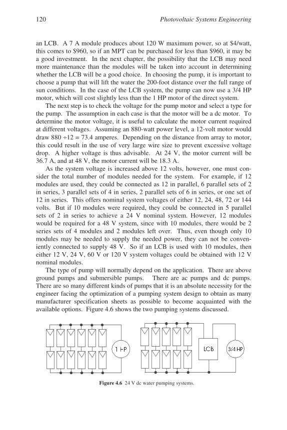
Photovoltaic Systems Engineering120
an LCB. A 7 A module produces about 120 W maximum power, so at $4/watt,this comes to $960, so if an MPT can be purchased for less than $960, it may bea good investment. In the next chapter, the possibility that the LCB may needmore maintenance than the modules will be taken into account in determiningwhether the LCB will be a good choice. In choosing the pump, it is important tochoose a pump that will lift the water the 200-foot distance over the full range ofsun conditions. In the case of the LCB system, the pump can now use a 3/4 HPmotor, which will cost slightly less than the 1 HP motor of the direct system.
The next step is to check the voltage for the pump motor and select a type forthe pump. The assumption in each case is that the motor will be a dc motor. Todetermine the motor voltage, it is useful to calculate the motor current requiredat different voltages. Assuming an 880-watt power level, a 12-volt motor woulddraw 880 ÷12 = 73.4 amperes. Depending on the distance from array to motor,this could result in the use of very large wire size to prevent excessive voltagedrop. A higher voltage is thus advisable. At 24 V, the motor current will be36.7 A, and at 48 V, the motor current will be 18.3 A.
As the system voltage is increased above 12 volts, however, one must con-sider the total number of modules needed for the system. For example, if 12modules are used, they could be connected as 12 in parallel, 6 parallel sets of 2in series, 3 parallel sets of 4 in series, 2 parallel sets of 6 in series, or one set of12 in series. This offers nominal system voltages of either 12, 24, 48, 72 or 144volts. But if 10 modules were required, they could be connected in 5 parallelsets of 2 in series to achieve a 24 V nominal system. However, 12 moduleswould be required for a 48 V system, since with 10 modules, there would be 2series sets of 4 modules and 2 modules left over. Thus, even though only 10modules may be needed to supply the needed power, they can not be conven-iently connected to supply 48 V. So if an LCB is used with 10 modules, theneither 12 V, 24 V, 60 V or 120 V system voltages could be obtained with 12 Vnominal modules.
The type of pump will normally depend on the application. There are aboveground pumps and submersible pumps. There are ac pumps and dc pumps.There are so many different kinds of pumps that it is an absolute necessity for theengineer facing the optimization of a pumping system design to obtain as manymanufacturer specification sheets as possible to become acquainted with theavailable options. Figure 4.6 shows the two pumping systems discussed.
Figure 4.6 24 V dc water pumping systems.
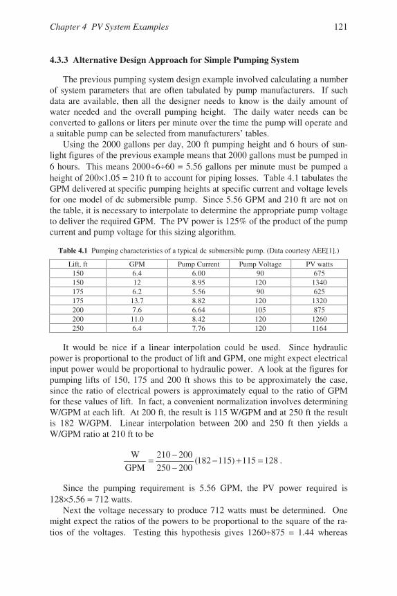
Chapter 4 PV System Examples 121
4.3.3 Alternative Design Approach for Simple Pumping System
The previous pumping system design example involved calculating a numberof system parameters that are often tabulated by pump manufacturers. If suchdata are available, then all the designer needs to know is the daily amount ofwater needed and the overall pumping height. The daily water needs can beconverted to gallons or liters per minute over the time the pump will operate anda suitable pump can be selected from manufacturers’ tables.
Using the 2000 gallons per day, 200 ft pumping height and 6 hours of sun-light figures of the previous example means that 2000 gallons must be pumped in6 hours. This means 2000÷6÷60 = 5.56 gallons per minute must be pumped aheight of 200×1.05 = 210 ft to account for piping losses. Table 4.1 tabulates theGPM delivered at specific pumping heights at specific current and voltage levelsfor one model of dc submersible pump. Since 5.56 GPM and 210 ft are not onthe table, it is necessary to interpolate to determine the appropriate pump voltageto deliver the required GPM. The PV power is 125% of the product of the pumpcurrent and pump voltage for this sizing algorithm.
Table 4.1 Pumping characteristics of a typical dc submersible pump. (Data courtesy AEE[1].)
Lift, ft GPM Pump Current Pump Voltage PV watts150 6.4 6.00 90 675150 12 8.95 120 1340175 6.2 5.56 90 625175 13.7 8.82 120 1320200 7.6 6.64 105 875200 11.0 8.42 120 1260250 6.4 7.76 120 1164
It would be nice if a linear interpolation could be used. Since hydraulicpower is proportional to the product of lift and GPM, one might expect electricalinput power would be proportional to hydraulic power. A look at the figures forpumping lifts of 150, 175 and 200 ft shows this to be approximately the case,since the ratio of electrical powers is approximately equal to the ratio of GPMfor these values of lift. In fact, a convenient normalization involves determiningW/GPM at each lift. At 200 ft, the result is 115 W/GPM and at 250 ft the resultis 182 W/GPM. Linear interpolation between 200 and 250 ft then yields aW/GPM ratio at 210 ft to be
128115)115182(200250
200210
GPM
W =+−−−= .
Since the pumping requirement is 5.56 GPM, the PV power required is128×5.56 = 712 watts.
Next the voltage necessary to produce 712 watts must be determined. Onemight expect the ratios of the powers to be proportional to the square of the ra-tios of the voltages. Testing this hypothesis gives 1260÷875 = 1.44 whereas
Photovoltaic Systems Engineering122
(120÷105)2 = 1.31, suggesting perhaps a different power relationship. If it istrue that
,V
V
P
Pn
1
2
1
2⎟⎟⎠
⎞⎜⎜⎝
⎛= (4.2)
then one can solve for n, using 1260 and 875 for P2 and P1 and 120 and 105 forV2 and V1. The result (see Problem 4.3) is n = 2.73. Now, n = 2.73 is used inestimating the operating voltage associated with the 712 watts of PV powerneeded to pump the 5.56 GPM through the 210-ft lift. The voltage, V2, can bedetermined by substituting P2 = 712 W, P1 = 875 W and V1 = 105 V into (4.2),with n = 2.73. The result (see Problem 4.3) is V2 = 97.4 V. Hence, ifV2 = 97.4 V, the PV current must be 712÷97.4 = 7.31 A.
For modules rated at Vmp = 17 V and Imp = 7.3 A, one might expect that con-necting 6 of these modules in series would be adequate, since the output atmaximum power should be 7.3 A at 102 V, or 745 W. In a perfect world, thiswould be true, but because of temperature and other degradation factors, pumpmanufacturers generally recommend oversizing the PV array by 25%. Hence, toensure adequate current, it would be better to connect 7 modules in series. Fur-thermore, pump manufacturers generally recommend using an LCB with thepump, so the final system should probably also use a LCB for better performanceat lower light levels and to better match the array characteristic to the pumpcharacteristic.
One should note, however, that the cost of this 1 HP pump is over $1800,whereas a 1/4 HP pump that will deliver 2.15 GPM while consuming 186 wattscan be purchased for $495. This suggests the entire system, including the batterystorage needed for the slower pumping rate should probably be evaluated when aserious design exercise is in progress.
Other manufacturers provide tables for their pumps that list lift, GPM andpower consumed for a fixed pump voltage. These tables are very convenient andresult in simple interpolations and reliable results, especially if pump voltage ismaintained nearly constant with batteries.
4.4 Example 3: A PV-Powered Area Lighting System
4.4.1 Determination of the Lighting Load
The design of a PV-powered area lighting system follows closely the designof the fan system with battery backup. The first step is to determine the lightingload, followed with battery selection and, finally, the number and type of PVmodules to use. In order to determine the lighting load in watts, it is first neces-sary to determine the amount of light needed and the area over which the light isneeded. Hence, the design begins with the determination of the necessary illu-mination level.
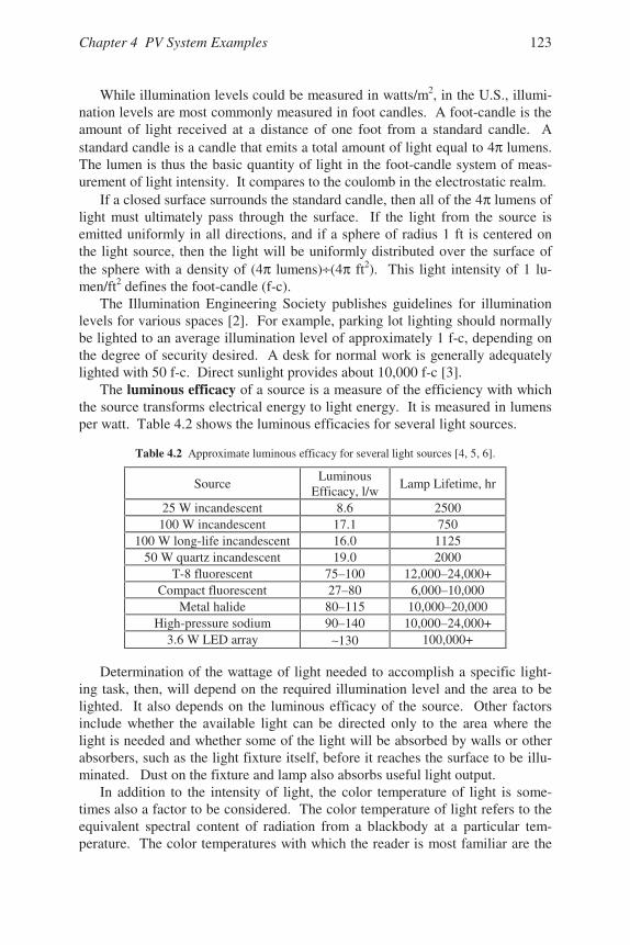
Chapter 4 PV System Examples 123
While illumination levels could be measured in watts/m2, in the U.S., illumi-nation levels are most commonly measured in foot candles. A foot-candle is theamount of light received at a distance of one foot from a standard candle. Astandard candle is a candle that emits a total amount of light equal to 4π lumens.The lumen is thus the basic quantity of light in the foot-candle system of meas-urement of light intensity. It compares to the coulomb in the electrostatic realm.
If a closed surface surrounds the standard candle, then all of the 4π lumens oflight must ultimately pass through the surface. If the light from the source isemitted uniformly in all directions, and if a sphere of radius 1 ft is centered onthe light source, then the light will be uniformly distributed over the surface ofthe sphere with a density of (4π lumens)÷(4π ft2). This light intensity of 1 lu-men/ft2 defines the foot-candle (f-c).
The Illumination Engineering Society publishes guidelines for illuminationlevels for various spaces [2]. For example, parking lot lighting should normallybe lighted to an average illumination level of approximately 1 f-c, depending onthe degree of security desired. A desk for normal work is generally adequatelylighted with 50 f-c. Direct sunlight provides about 10,000 f-c [3].
The luminous efficacy of a source is a measure of the efficiency with whichthe source transforms electrical energy to light energy. It is measured in lumensper watt. Table 4.2 shows the luminous efficacies for several light sources.
Table 4.2 Approximate luminous efficacy for several light sources [4, 5, 6].
SourceLuminous
Efficacy, l/wLamp Lifetime, hr
25 W incandescent 8.6 2500100 W incandescent 17.1 750
100 W long-life incandescent 16.0 112550 W quartz incandescent 19.0 2000
T-8 fluorescent 75–100 12,000–24,000+Compact fluorescent 27–80 6,000–10,000
Metal halide 80–115 10,000–20,000High-pressure sodium 90–140 10,000–24,000+
3.6 W LED array ∼130 100,000+
Determination of the wattage of light needed to accomplish a specific light-ing task, then, will depend on the required illumination level and the area to belighted. It also depends on the luminous efficacy of the source. Other factorsinclude whether the available light can be directed only to the area where thelight is needed and whether some of the light will be absorbed by walls or otherabsorbers, such as the light fixture itself, before it reaches the surface to be illu-minated. Dust on the fixture and lamp also absorbs useful light output.
In addition to the intensity of light, the color temperature of light is some-times also a factor to be considered. The color temperature of light refers to theequivalent spectral content of radiation from a blackbody at a particular tem-perature. The color temperatures with which the reader is most familiar are the
Photovoltaic Systems Engineering124
5800 K temperature of the sun, which produces its characteristic white color, andthe 3000 K temperature of a tungsten incandescent light filament, which is moretoward orange. Not all light sources can be characterized by a color tempera-ture, since the concept is based on blackbody radiators. Sources with discretespectral components, such as lasers or gas discharge lamps, can be assignedequivalent color temperatures to indicate the temperature to which the spectrumof the source is most closely matched, but the color temperature is not a precisemeasure of the color of the source. For example, xenon produces a very whiteflash, which, on photographic film, appears to be close to the color of daylight.Although the output spectrum of a xenon lamp differs from the AM 1.5 solarspectrum, xenon lamps are commonly used in solar simulators with appropriatecorrection factors.
Consideration of color temperature can be an important factor in the choiceof light sources. For example, low pressure sodium has a very high luminousefficacy, but the light is comprised primarily of the sodium d2 lines. When lowpressure sodium sources are used, anything not yellow in color will not be accu-rately perceived, since, if a source does not contain a particular color, then thatcolor cannot be reflected back to the eye to be perceived as such. For PV appli-cations, generally the most popular and efficient sources are fluorescent, metalhalide and high pressure sodium. Occasionally incandescent sources are usedfor special purpose applications.
4.4.2 An Outdoor Lighting System
Suppose it is desired to provide nominal lighting in an area to enable peopleto see a walkway and any animals that may have come into the area. An averageillumination level of approximately 1 f-c can do this. Suppose the area to belighted is 15 feet wide and 1000 feet long and suppose a sharp cut-off fixture hasbeen found that will provide coverage for an area measuring 15 feet by 40 feet ifmounted on a 10-foot pole. The fixture has a coefficient of utilization (CU) of0.80, which means that 80% of the light produced by the lamp will emerge fromthe fixture. Note that this CU is valid provided that the fixture remains clean.The maintenance factor (MF) (0 < MF < 1) accounts for dirt on the lamp, lensand reflector. One could thus estimate further reduction in light directed towardthe designated space with another correction factor.
First, the number of fixtures must be determined. This is simple in this case,since each fixture will light 40 feet of the total length. Thus 25 fixtures will beneeded, spaced at 40-foot intervals. Note that this spacing, four pole heightsapart, is common for area lighting systems. Since the fixtures will be PV pow-ered, each will be self-contained and can be specified separately. Hence, thesolution for a 15-by-40-foot area will simply be repeated 25 times.
The total lumen requirement for each fixture is determined by the product ofthe area lighted and the average illumination level. In this case the result is 600ft2 × 1 f-c = 600 lumens. Since the CU of the fixture is 0.8, the lumen output of
Chapter 4 PV System Examples 125
the lamp must be 600÷0.8 = 750 lumens. This is close to the light output of a 9-watt compact fluorescent tube, which will produce approximately 600 lumens.Since the illumination level is not critical, the 9-watt tube should be adequate.
If the walkway is to remain lighted all night, it is necessary to determine thelongest night of the year. Suppose the longest winter night is 15 hours. Thismeans the shortest summer night will be 9 hours. It also means that the PVmodules on the shortest day of the year must produce enough electricity to oper-ate the fixtures through the longest night of the year. On the other hand, duringthe longest day, the PV array only need produce enough electricity for the short-est night. Clearly, if the longest night demand is to be met, the system will wasteelectricity during the longest day. Depending on the application or the location,it may be possible to either turn off the lights for a few hours during the longestnight or to find an alternate use for the excess energy during the longest days.
Next, suppose a 12-volt system is selected. This means the lamps will draw0.75 A when they are operating. The worst case daily corrected load is thus15×0.75÷0.9÷0.98 = 12.76 Ah. Suppose 3 days of storage are required anddeep-cycle batteries are used. This means that 12.76×3÷0.8 = 47.9 Ah of stor-age is needed, assuming a depth of discharge of 80%. So a single 12 V batterywith a minimum capacity of 48 Ah can be used.
To size the PV array, the peak sun hours of the shortest day are needed.Suppose the winter peak sun is 4 hours and the summer peak sun is 6 hours.Thus, in 4 hours, the array must produce 12.76÷0.9 = 14.2 Ah. This means anhourly production rate of 3.55 Ah/h = 3.55 A. This can be done with a standardmodule rated at approximately 50 watts at maximum power, since the chargingwill be done at approximately 15 to 16 volts. A very straightforward system isthus possible, with a readily obtainable fixture, lamp, battery and module. Ofcourse, a means of switching the light on and off between dusk and dawn needsto be incorporated into the system. This may be a relay in series with the mod-ule, which keeps the light off as long as the battery is charging, but turns the lighton when the battery is no longer charging. A CdS photocell may be a more effi-cient choice of sensor, however, since the power loss in the relay coil duringcharging will probably exceed any minimal power loss in the photocell. Thecareful engineer will check both options.
It is interesting to look at the summer performance of the system. Since thelamp is on for only 9 hours per night, the daily corrected load is reduced to 9/15of the winter consumption, or 7.66 Ah. The module, on the other hand, will pro-duce 3.55×6×0.9 = 19.2 Ah. This means an excess of 11.5 Ah per day is pro-duced by the system. If this additional energy is directed to the battery, the bat-tery will soon become overcharged and its lifetime will be shortened. It is thusimportant to either employ another use for the excess summer energy or else toemploy a charge controller to limit the state of charge of the battery. It is alsointeresting to note that since the battery needs are nominal, a somewhat largerbattery can be obtained at a nominal additional cost, so that the winter storagecan be increased beyond 3 days.
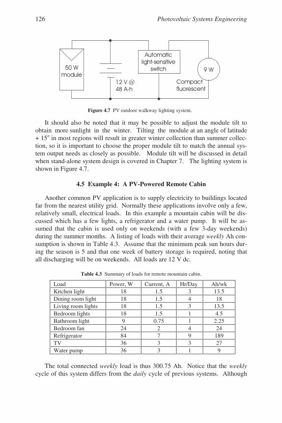
Photovoltaic Systems Engineering126
It should also be noted that it may be possible to adjust the module tilt toobtain more sunlight in the winter. Tilting the module at an angle of latitude+ 15o in most regions will result in greater winter collection than summer collec-tion, so it is important to choose the proper module tilt to match the annual sys-tem output needs as closely as possible. Module tilt will be discussed in detailwhen stand-alone system design is covered in Chapter 7. The lighting system isshown in Figure 4.7.
4.5 Example 4: A PV-Powered Remote Cabin
Another common PV application is to supply electricity to buildings locatedfar from the nearest utility grid. Normally these applications involve only a few,relatively small, electrical loads. In this example a mountain cabin will be dis-cussed which has a few lights, a refrigerator and a water pump. It will be as-sumed that the cabin is used only on weekends (with a few 3-day weekends)during the summer months. A listing of loads with their average weekly Ah con-sumption is shown in Table 4.3. Assume that the minimum peak sun hours dur-ing the season is 5 and that one week of battery storage is required, noting thatall discharging will be on weekends. All loads are 12 V dc.
Table 4.3 Summary of loads for remote mountain cabin.
Load Power, W Current, A Hr/Day Ah/wkKitchen light 18 1.5 3 13.5Dining room light 18 1.5 4 18Living room lights 18 1.5 3 13.5Bedroom lights 18 1.5 1 4.5Bathroom light 9 0.75 1 2.25Bedroom fan 24 2 4 24Refrigerator 84 7 9 189TV 36 3 3 27Water pump 36 3 1 9
The total connected weekly load is thus 300.75 Ah. Notice that the weeklycycle of this system differs from the daily cycle of previous systems. Although
!
Figure 4.7 PV outdoor walkway lighting system.
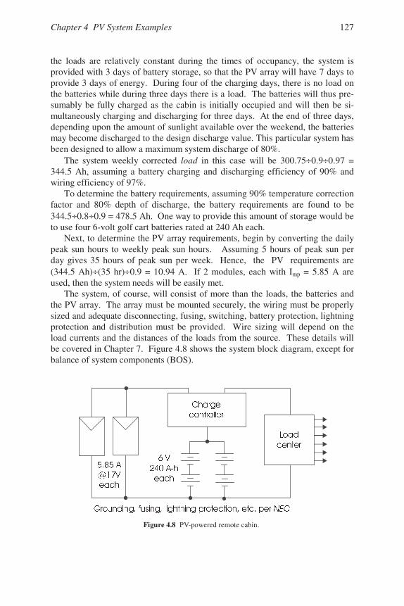
Chapter 4 PV System Examples 127
the loads are relatively constant during the times of occupancy, the system isprovided with 3 days of battery storage, so that the PV array will have 7 days toprovide 3 days of energy. During four of the charging days, there is no load onthe batteries while during three days there is a load. The batteries will thus pre-sumably be fully charged as the cabin is initially occupied and will then be si-multaneously charging and discharging for three days. At the end of three days,depending upon the amount of sunlight available over the weekend, the batteriesmay become discharged to the design discharge value. This particular system hasbeen designed to allow a maximum system discharge of 80%.
The system weekly corrected load in this case will be 300.75÷0.9÷0.97 =344.5 Ah, assuming a battery charging and discharging efficiency of 90% andwiring efficiency of 97%.
To determine the battery requirements, assuming 90% temperature correctionfactor and 80% depth of discharge, the battery requirements are found to be344.5÷0.8÷0.9 = 478.5 Ah. One way to provide this amount of storage would beto use four 6-volt golf cart batteries rated at 240 Ah each.
Next, to determine the PV array requirements, begin by converting the dailypeak sun hours to weekly peak sun hours. Assuming 5 hours of peak sun perday gives 35 hours of peak sun per week. Hence, the PV requirements are(344.5 Ah)÷(35 hr)÷0.9 = 10.94 A. If 2 modules, each with Imp = 5.85 A areused, then the system needs will be easily met.
The system, of course, will consist of more than the loads, the batteries andthe PV array. The array must be mounted securely, the wiring must be properlysized and adequate disconnecting, fusing, switching, battery protection, lightningprotection and distribution must be provided. Wire sizing will depend on theload currents and the distances of the loads from the source. These details willbe covered in Chapter 7. Figure 4.8 shows the system block diagram, except forbalance of system components (BOS).
!!
Figure 4.8 PV-powered remote cabin.
Photovoltaic Systems Engineering128
4.6 Example 5: A Hybrid System
Sometimes it is not economical or practical to provide all energy with PVmodules. For example, when loads are relatively constant during summer andwinter, or, perhaps even greater in winter, and if winter peak sun is very low, itmay take a large number of modules to meet winter requirements. This may re-sult in significant waste of energy produced by the modules during the summermonths. In such cases, it may be more economical to provide some of the sys-tem energy needs by another means, such as a gasoline or diesel generator. Asystem that uses PV for part of its energy production and other means for thebalance of the production is called a hybrid system. The best cost-effectivenessis generally obtained when none of the PV-generated energy is wasted.
Consider, for example, a radio repeater system at a high northern latitude thatreceives 7 hours of summer peak sun but only 1 hour of winter peak sun, with 3hours average peak sun for spring and fall. Assume the system requires a con-stant 2 kW for 24 hours per day all year long, and that a PV system is to handlethe summer load with 3 days of battery backup. Assume also that a gasoline gen-erator will deliver the balance of system needs and that the generator will gener-ate 6 kWh per gallon of fuel, and the system will only be refueled twice per year.The battery backup is important, since the system need is critical, and if the gen-erator should fail, 3 days of battery power are needed to allow time for generatorrepair. The radio equipment operates on 120 V ac, so an ac generator and aninverter will be used. The inverter will have internal provisions for charging thebatteries from the generator at an efficiency of 90%.
First, the corrected load is determined to be 2×24÷0.9÷0.98÷0.9 = 60.5kWh/day, where 90% battery utilization efficiency, 98% wiring efficiency and90% inverter efficiency are used. So the 60.5 kWh/day is the energy that mustbe delivered to the batteries. If the batteries operate at 48 volts, then thisamounts to a daily corrected load of (60,500 Wh)÷48 V = 1260 Ah.
Assuming a 90% PV array degradation factor and 7 peak sun hours, the arraycurrent must be 1260÷0.9÷7 = 200 A. Note that if the array were sized to meetthe winter load, then the array current would need to be 1400 A.
One popular larger module will deliver 17.4 A at 17.2 V [7]. Hence, to pro-duce 200 A at 17.2 V, it will take 200÷7.4 = 12 modules. Since it will take 4modules in series to produce the needed battery charging voltage of approxi-mately 56–58 V, 48 modules will be needed. Note that 48 modules will produce14,400 W if operated at maximum power at standard test conditions, whereas inthis system, with an output voltage of 56 V, the modules will only be producing11,700 W, or 81.2% of their rated output. This power loss is due to the fact thatthe modules are expected to operate at approximately 10–12 V below the stan-dard test condition Vmp.
Battery storage requirements are determined by dividing 60.5 kWh by thenominal system voltage, resulting in 1260 Ah per day of storage. Assuming useof deep-cycle batteries, but allowing for the batteries to cool down some in the
Chapter 4 PV System Examples 129
winter, resulting in less available charge, the total battery capacity required be-comes 1260×3÷0.9÷0.8 = 5250 Ah. The 0.9 factor represents the winter chargedegradation factor. If 6 V, 350 Ah batteries are used, then a total of 15 batteriesin parallel will be needed, and since it takes 8 batteries in series to produce 84volts, the total number of batteries increases to 120. Obviously this system is abit larger than the systems previously discussed. For this system, it makes muchbetter sense to use larger, sealed, maintenance-free batteries, such as a 1055 Ah@ 12 V unit [14]. The system will require 20 of these batteries.
The total energy requirement of the battery system is (5250 Ah)×(48 V) =252,000 Wh = 252 kWh. If the generator is to charge the batteries at a rate ofC/10, the generator must be rated at (252 kWh)÷(10 hr) = 25.2 kW. Taking intoaccount a 90% conversion efficiency from generator ac output to battery dc in-put, a 28 kW generator will just meet the desired C/10 rate. Since the C/10 rateis not critical, a 25 kW generator will be adequate for the job.
The next items to be determined are the annual fuel usage and generator run-ning time. To do so involves estimating the fraction of the total energy needsthat should be produced by the PV array.
With the information given, the assumption is that for 3 months, the PV sys-tem produces all of the system electrical needs. Then, for 6 months the PV sys-tem provides only 3/7 of the system needs, since the peak sun hours are reducedfrom 7 to 3 during spring and fall. During the winter 3 months, the PV systemwill only supply 1/7 of the system needs.
Hence, for 182 days, the generator must produce (4/7)×60.5÷0.9 = 38.4kWh/day, which results in 182×38.4 = 6989 total kWh production. The 0.9factor is included to compensate for the loss in conversion of ac to dc for charg-ing. For the winter months, the generator must provide (6/7)×60.5÷0.9 = 57.6kWh/day for 91 days. This amounts to 5242 kWh. The total annual generatorelectrical output is thus 12,231 kWh.
Now, since the generator will produce 6 kWh/gal, the generator annual gaso-line consumption will be 2039 gallons. If the tank is filled twice per year, then atank half that size will suffice. To provide a slight safety margin, a 1200 gallontank would be a reasonable choice. At a worst-case consumption rate of 57.6÷6= 9.6 gal/day, this provides about an 18.8-day leeway in case of bad weather orother problems in accessing the site for gasoline delivery.
To determine the generator run time per year for maintenance purposes, notethat the generator produces 25 kW while it is operating, on the average. Forexample, depending on the control system, if the PV system is providing part ormost of the power needed by the repeater system, depending on the state ofcharge of the batteries, the generator may or may not be running. Without thisinformation on the control algorithm, it is only possible to deal with averages.Hence, dividing the kWh by the kW yields the hours of operation. The result is489 hours of operation per year.
Without the PV system, the generator would have to generate 365×60.5÷0.9= 24,536 kWh/yr. The PV system thus saves 12,305 kWh of generation by the
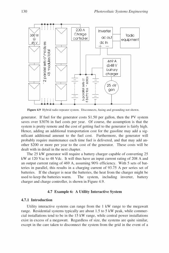
Photovoltaic Systems Engineering130
generator. If fuel for the generator costs $1.50 per gallon, then the PV systemsaves over $3076 in fuel costs per year. Of course, the assumption is that thesystem is pretty remote and the cost of getting fuel to the generator is fairly high.Hence, adding an additional transportation cost for the gasoline may add a sig-nificant additional amount to the fuel cost. Furthermore, the generator willprobably require maintenance each time fuel is delivered, and that may add an-other $200 or more per year to the cost of the generator. These costs will bedealt with in detail in the next chapter.
The 25 kW generator will require a battery charger capable of converting 25kW at 120 Vac to 48 Vdc. It will thus have an input current rating of 208 A andan output current rating of 469 A, assuming 90% efficiency. With 5 sets of bat-teries in parallel, this results in a charging current of 93.75 A per series set ofbatteries. If the charger is near the batteries, the heat from the charger might beused to keep the batteries warm. The system, including inverter, batterycharger and charge controller, is shown in Figure 4.9.
4.7 Example 6: A Utility Interactive System
4.7.1 Introduction
Utility interactive systems can range from the 1 kW range to the megawattrange. Residential systems typically are about 1.5 to 5 kW peak, while commer-cial installations tend to be in the 15 kW range, while central power installationsexist in excess of a megawatt. Regardless of size, the systems are quite similar,except in the care taken to disconnect the system from the grid in the event of a
Figure 4.9 Hybrid radio repeater system. Disconnects, fusing and grounding not shown.
"!!
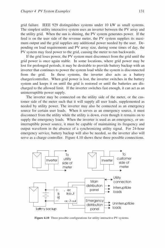
Chapter 4 PV System Examples 131
grid failure. IEEE 929 distinguishes systems under 10 kW as small systems.The simplest utility interactive system uses an inverter between the PV array andthe utility grid. When the sun is shining, the PV system generates power. If thefeed is on the user side of the revenue meter, the PV system supplies its maxi-mum output and the grid supplies any additional power needed by the user. De-pending on load requirements and PV array size, during some times of day, thePV system may feed power to the grid, causing the meter to run backwards.
If the grid loses power, the PV system must disconnect from the grid until thegrid power is once again stable. In some locations, where grid power may belost for prolonged periods, it may be desirable to provide battery backup with aninverter that continues to power the system load while the system is disconnectedfrom the grid. In these systems, the inverter also acts as a batterycharger/controller. When grid power is lost, the inverter switches in the batterysystem and keeps it on until the grid is restored or until the batteries are dis-charged to the allowed limit. If the inverter switches fast enough, it can act as anuninterruptible power supply.
The inverter may be connected on the utility side of the meter, or the cus-tomer side of the meter such that it will supply all user loads, supplemented asneeded by utility power. The inverter may also be connected as an emergencysource for certain user loads. When it serves as an emergency source, it mustdisconnect from the utility while the utility is down, even though it remains on tosupply the emergency loads. When the inverter is used as an emergency, or un-interruptible power source, it must be capable of maintaining its frequency andoutput waveform in the absence of a synchronizing utility signal. For 24-houremergency service, battery backup will also be needed, so the inverter also willserve as a charge controller. Figure 4.10 shows these three possible connections.
"!! "!!
#$
!
#!
!
%$
"!!&
%!!&
Figure 4.10 Three possible configurations for utility interactive PV systems.
'!&
(!$!&
Photovoltaic Systems Engineering132
4.7.2 A Simple Utility Interactive System with No Battery Storage
One nice feature of a utility interactive system is that if it does not have aspecific backup function, the amount of PV installed depends upon the spaceavailable for the array and the budget of the system owner. If the PV array isconnected to the customer side of the meter and if the array is generating in ex-cess of customer needs, the excess is fed into the grid. If the PV is not meetingthe needs of the customer, then the grid meets these needs. The origin of theelectricity is transparent to the customer.
As long as the PV system does not generate more energy than the customeruses at any moment, the presence of the PV system will be similar to the imple-mentation of a conservation measure—it simply lowers the customer’s monthlyelectric bill. An interesting situation occurs, however, if the PV system gener-ates more than the customer’s needs at any moment during a metering period. Inthis case, the utility must determine a price for which to purchase the excess PVenergy. If the utility does not own the PV system, then the question becomeswhether to purchase the excess electrical energy at wholesale or retail prices.Herein lies a question, that of net metering, that may remain unanswered untilvarious regulatory bodies study the pros and cons of each possibility. As thisedition goes to press, 34 states have enacted net metering laws that require theutility to purchase the power from the PV power producer at the same rate that ischarged the producer for electricity used from the utility [8].
From a technical perspective, however, the installation is simple, providedthat the inverter is listed to comply with UL 1741, meaning that it meets IEEE929 standards and that it complies with the requirements of the National Electri-cal Code, which requires all utility interactive inverters to be UL 1741 listed.The system also needs to be installed in accordance with all NEC requirements,including fusing, switching, ground fault protection and disconnects. Note thatthese conditions apply to PV arrays less than 10 kW.
As an example system, consider a 2400 W PV array, connected appropriatelyto a 2500 W inverter. The PV array has 20 modules rated at 120 W each, withmodule Vmp = 16.9 V, VOC = 21.5 V, Imp = 7.10 A and ISC = 7.45 A. The mod-ules are connected in a single series source circuit that delivers 7.10 A at 338 Vdc under standard test conditions, provided that the inverter tracks array maxi-mum power.
The inverter is line commutated so it depends on the utility voltage for syn-chronism. It has a 240 V, single phase, output voltage and feeds into the mainpanel of a dwelling through a 2-pole 20 A circuit breaker. The inverter inputtracks maximum array power over an input voltage range of 225 to 550 V dc at amaximum inverter input current of 10.5 A.
Note that the inverter output is connected to the load side of the circuitbreaker, since the line side of the breaker is connected to the bus bar of the mainpanel that is fed from the utility connection. Thus, when the circuit breaker isturned off, it is still conceivable that both sides of the breaker may be live, since
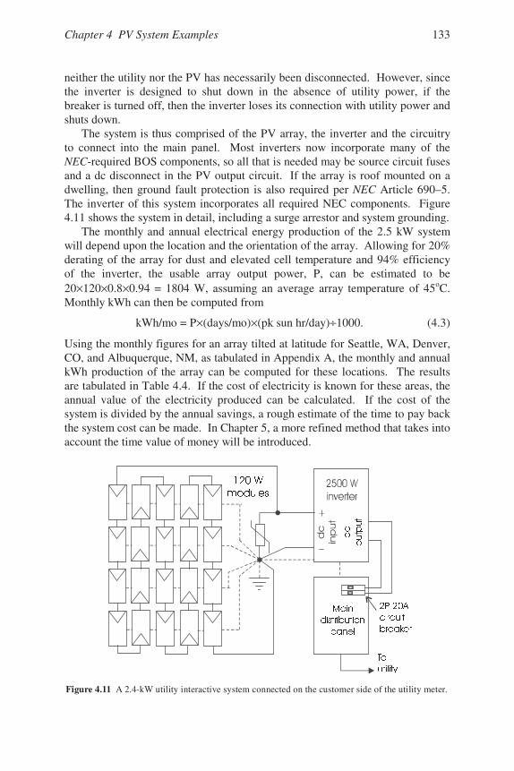
Chapter 4 PV System Examples 133
neither the utility nor the PV has necessarily been disconnected. However, sincethe inverter is designed to shut down in the absence of utility power, if thebreaker is turned off, then the inverter loses its connection with utility power andshuts down.
The system is thus comprised of the PV array, the inverter and the circuitryto connect into the main panel. Most inverters now incorporate many of theNEC-required BOS components, so all that is needed may be source circuit fusesand a dc disconnect in the PV output circuit. If the array is roof mounted on adwelling, then ground fault protection is also required per NEC Article 690–5.The inverter of this system incorporates all required NEC components. Figure4.11 shows the system in detail, including a surge arrestor and system grounding.
The monthly and annual electrical energy production of the 2.5 kW systemwill depend upon the location and the orientation of the array. Allowing for 20%derating of the array for dust and elevated cell temperature and 94% efficiencyof the inverter, the usable array output power, P, can be estimated to be20×120×0.8×0.94 = 1804 W, assuming an average array temperature of 45oC.Monthly kWh can then be computed from
kWh/mo = P×(days/mo)×(pk sun hr/day)÷1000. (4.3)
Using the monthly figures for an array tilted at latitude for Seattle, WA, Denver,CO, and Albuquerque, NM, as tabulated in Appendix A, the monthly and annualkWh production of the array can be computed for these locations. The resultsare tabulated in Table 4.4. If the cost of electricity is known for these areas, theannual value of the electricity produced can be calculated. If the cost of thesystem is divided by the annual savings, a rough estimate of the time to pay backthe system cost can be made. In Chapter 5, a more refined method that takes intoaccount the time value of money will be introduced.
Figure 4.11 A 2.4-kW utility interactive system connected on the customer side of the utility meter.
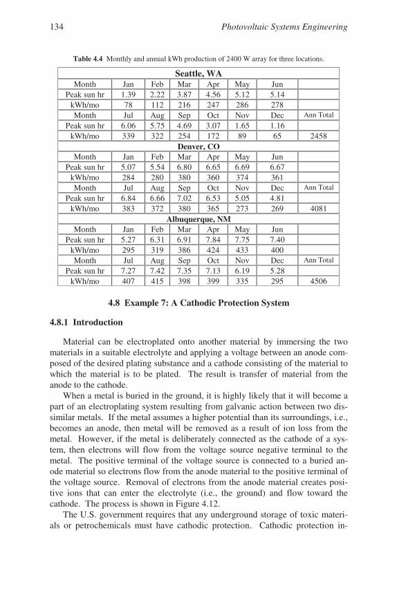
Photovoltaic Systems Engineering134
Table 4.4 Monthly and annual kWh production of 2400 W array for three locations.
Seattle, WAMonth Jan Feb Mar Apr May Jun
Peak sun hr 1.39 2.22 3.87 4.56 5.12 5.14kWh/mo 78 112 216 247 286 278Month Jul Aug Sep Oct Nov Dec Ann Total
Peak sun hr 6.06 5.75 4.69 3.07 1.65 1.16kWh/mo 339 322 254 172 89 65 2458
Denver, COMonth Jan Feb Mar Apr May Jun
Peak sun hr 5.07 5.54 6.80 6.65 6.69 6.67kWh/mo 284 280 380 360 374 361Month Jul Aug Sep Oct Nov Dec Ann Total
Peak sun hr 6.84 6.66 7.02 6.53 5.05 4.81kWh/mo 383 372 380 365 273 269 4081
Albuquerque, NMMonth Jan Feb Mar Apr May Jun
Peak sun hr 5.27 6.31 6.91 7.84 7.75 7.40kWh/mo 295 319 386 424 433 400Month Jul Aug Sep Oct Nov Dec Ann Total
Peak sun hr 7.27 7.42 7.35 7.13 6.19 5.28kWh/mo 407 415 398 399 335 295 4506
4.8 Example 7: A Cathodic Protection System
4.8.1 Introduction
Material can be electroplated onto another material by immersing the twomaterials in a suitable electrolyte and applying a voltage between an anode com-posed of the desired plating substance and a cathode consisting of the material towhich the material is to be plated. The result is transfer of material from theanode to the cathode.
When a metal is buried in the ground, it is highly likely that it will become apart of an electroplating system resulting from galvanic action between two dis-similar metals. If the metal assumes a higher potential than its surroundings, i.e.,becomes an anode, then metal will be removed as a result of ion loss from themetal. However, if the metal is deliberately connected as the cathode of a sys-tem, then electrons will flow from the voltage source negative terminal to themetal. The positive terminal of the voltage source is connected to a buried an-ode material so electrons flow from the anode material to the positive terminal ofthe voltage source. Removal of electrons from the anode material creates posi-tive ions that can enter the electrolyte (i.e., the ground) and flow toward thecathode. The process is shown in Figure 4.12.
The U.S. government requires that any underground storage of toxic materi-als or petrochemicals must have cathodic protection. Cathodic protection in-
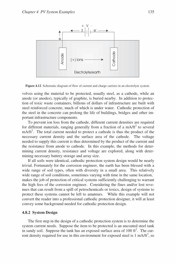
Chapter 4 PV System Examples 135
volves using the material to be protected, usually steel, as a cathode, while ananode (or anodes), typically of graphite, is buried nearby. In addition to protec-tion of toxic waste containers, billions of dollars of infrastructure are built withsteel reinforced concrete, much of which is under water. Cathodic protection ofthe steel in the concrete can prolong the life of buildings, bridges and other im-portant infrastructure components.
To prevent ion loss from the cathode, different current densities are requiredfor different materials, ranging generally from a fraction of a mA/ft2 to severalmA/ft2. The total current needed to protect a cathode is thus the product of thenecessary current density and the surface area of the cathode. The voltageneeded to supply this current is thus determined by the product of the current andthe resistance from anode to cathode. In this example, the methods for deter-mining current density, resistance and voltage are explored, along with deter-mining necessary battery storage and array size.
If all soils were identical, cathodic protection system design would be nearlytrivial. Fortunately for the corrosion engineer, the earth has been blessed with awide range of soil types, often with diversity in a small area. This relativelywide range of soil conditions, sometimes varying with time in the same location,makes the job of protection of critical systems sufficiently challenging to warrantthe high fees of the corrosion engineer. Considering the fines and/or lost reve-nues that can result from a spill of petrochemicals or toxics, design of systems toprotect these systems cannot be left to amateurs. While this example will notconvert the reader into a professional cathodic protection designer, it will at leastconvey some background needed for cathodic protection design.
4.8.2 System Design
The first step in the design of a cathodic protection system is to determine thesystem current needs. Suppose the item to be protected is an uncoated steel tankin sandy soil. Suppose the tank has an exposed surface area of 100 ft2. The cur-rent density required for use in this environment for exposed steel is 1 mA/ft2, so
I
Figure 4.12 Schematic diagram of flow of current and charge carriers in an electrolyte system.
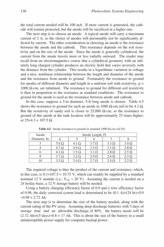
Photovoltaic Systems Engineering136
the total current needed will be 100 mA. If more current is generated, the cath-ode will remain protected, but the anode will be sacrificed at a higher rate.
The next step is to choose an anode. A typical anode will carry a maximumcurrent of 2 A, so the choice of anodes will presumably not be significantly af-fected by current. The other consideration in choosing an anode is the resistancebetween the anode and the cathode. This resistance depends on the soil resis-tivity and on the size of the anode. Since the anode is generally cylindrical, thecurrent from the anode travels more or less radially outward. The reader mayrecall from an electromagnetics course that a cylindrical geometry with an infi-nitely long charged cylinder produces an electric field that varies inversely withthe distance from the cylinder. This results in a logarithmic variation in voltageand a nice, nonlinear relationship between the length and diameter of the anodeand the resistance from anode to ground. Fortunately the resistance to groundfor anodes of different diameter and length in a uniform soil with resistivity, ρ =1000 Ω-cm, are tabulated. The resistance to ground for different soil resistivityis then in proportion to the resistance at standard conditions. The resistance toground for the anode is used as the resistance between anode and cathode.
In this case, suppose a 3-in diameter, 5-ft long anode is chosen. Table 4.5shows the resistance to ground for such an anode in 1000 Ω But the resistivity of sandy soil is closer to 25,000 Ω-cm, so the resistance toground of this anode at the tank location will be approximately 25 times higher,or 25×4.3 = 107.5 Ω.
Table 4.5 Anode resistance to ground in standard 1000 Ω-cm soil [9].
Anode Length, FtAnodeDiameter, In 4 5 6 7 8
3 4 6 8
10
The required voltage is thus the product of the current and resistance, which,in this case, is 0.1×107.5 = 10.75 V, which can readily be supplied by a standardnominal 12 V module (i.e., VOC ≈ 20 V). Assuming the current is needed on a24 hr/day basis, a 12 V storage battery will be needed.
Using a battery charging efficiency factor of 0.9 and a wire efficiency factorof 0.98, the daily corrected system load is determined to be (0.1 A)×(24 hr)÷0.9÷0.98 = 2.72 Ah.
The next step is to determine the size of the battery needed, along with thecurrent rating of the PV array. Assuming deep discharge batteries with 5 days ofstorage time and an allowable discharge of 80%, the battery needs will be(2.72 Ah)×(5 days)÷0.8 = 17 Ah. This is about the size of the battery in a smalluninterruptible power supply for computer backup power.

Chapter 4 PV System Examples 137
Finally, if the minimum daily insolation for the location of the tank is 4hours, using a module derating of 90%, the module current is found to be(2.72 Ah)÷(4 hr)÷0.9 = 0.76 A.
The module can thus be a 10-watt, 12-volt unit, and the battery can be asmall battery. However, if the maximum sun is significantly more than 4 hours,then the battery may overcharge, so a charge controller will be needed.
One might expect an alternative to a charge controller may be to use a largerbattery. However, with an excess of 2 or more Ah/day from the module, in 30days time, the battery will accumulate an additional 60 Ah. Only if the batteryloses charge over time with no load or if it is significantly oversized, will thebattery be safe from overcharge. Specifically, the NEC requires a charge con-troller whenever the PV array provides more than 3% of the battery rating in asingle day. This, of course, would apply to the highest average peak sun hoursof the year, whereas the present calculation has been based upon the lowest aver-age peak sun hours of the year.
Suppose the combination of protection current and anode resistance toground had resulted in the need for more than 12 volts. Several means of solv-ing this problem are available. One is simply to use modules in series. Anotheris to use a larger anode or to use anodes in parallel. One might expect an anodewith twice the surface area to have half the resistance to ground, but due to thenonlinearities of the system, this is not the case, as shown in Table 4.6.
The parallel anode solution results in a lower resistance to ground, but, per-haps not surprisingly, the resistance to ground of two identical anodes is notsimply half the resistance of a single anode. The cylindrical geometry againadds a nonlinear twist to the problem, resulting in the resistance to ground of twoanodes depending on the separation of the anodes. Table 4.6 shows multipleanode adjustment factors, assuming all anodes are identical and that the soil isuniform in composition. The factors in the table are multipliers for the singleanode resistance to ground. Thus, for example, if the resistance to ground for asingle anode is 100 Ω, then the resistance to ground for 3 anodes spaced 15 ftapart will be 100×0.418 = 41.8 Ω. This reduces the voltage required to 41.8%of that required for a single anode. It is thus a matter of calculating the life cyclecost (coming up in Chapter 5) of the three-anode system vs. the single anodesystem. Keeping in mind that each anode now will only carry 1/3 of the systemcurrent, the anodes should last three times longer.
A somewhat more elegant solution to the problem would involve an elec-tronic constant current source that would provide the required current regardlessof soil conditions or PV output. However, wet soil requires more current thandry soil, so the current source would need to be compensated for soil resistivity,rendering the current source design somewhat more challenging.
Whenever possible, it is advisable to make soil resistance measurements soempirical data can be used to size and locate system components properly. Thiseliminates many of the assumptions made and provides for greater confidence inthe performance of the system. Figure 4.13 shows the final system.
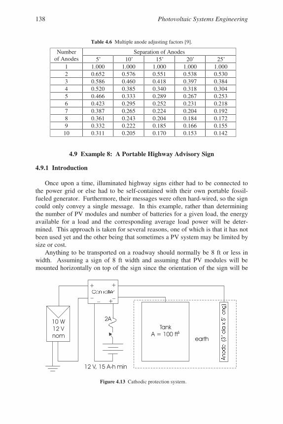
Photovoltaic Systems Engineering138
Table 4.6 Multiple anode adjusting factors [9].
Separation of AnodesNumberof Anodes 5’ 10’ 15’ 20’ 25’
1 1.000 1.000 1.000 1.000 1.0002 0.652 0.576 0.551 0.538 0.5303 0.586 0.460 0.418 0.397 0.3844 0.520 0.385 0.340 0.318 0.3045 0.466 0.333 0.289 0.267 0.2536 0.423 0.295 0.252 0.231 0.2187 0.387 0.265 0.224 0.204 0.1928 0.361 0.243 0.204 0.184 0.1729 0.332 0.222 0.185 0.166 0.155
10 0.311 0.205 0.170 0.153 0.142
4.9 Example 8: A Portable Highway Advisory Sign
4.9.1 Introduction
Once upon a time, illuminated highway signs either had to be connected tothe power grid or else had to be self-contained with their own portable fossil-fueled generator. Furthermore, their messages were often hard-wired, so the signcould only convey a single message. In this example, rather than determiningthe number of PV modules and number of batteries for a given load, the energyavailable for a load and the corresponding average load power will be deter-mined. This approach is taken for several reasons, one of which is that it has notbeen used yet and the other being that sometimes a PV system may be limited bysize or cost.
Anything to be transported on a roadway should normally be 8 ft or less inwidth. Assuming a sign of 8 ft width and assuming that PV modules will bemounted horizontally on top of the sign since the orientation of the sign will be
! "
#"
Figure 4.13 Cathodic protection system.
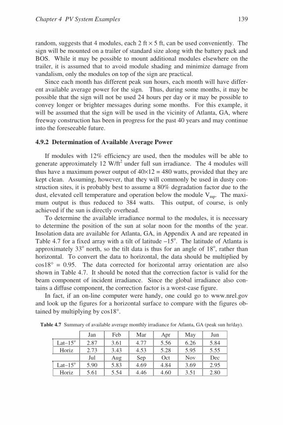
Chapter 4 PV System Examples 139
random, suggests that 4 modules, each 2 ft × 5 ft, can be used conveniently. Thesign will be mounted on a trailer of standard size along with the battery pack andBOS. While it may be possible to mount additional modules elsewhere on thetrailer, it is assumed that to avoid module shading and minimize damage fromvandalism, only the modules on top of the sign are practical.
Since each month has different peak sun hours, each month will have differ-ent available average power for the sign. Thus, during some months, it may bepossible that the sign will not be used 24 hours per day or it may be possible toconvey longer or brighter messages during some months. For this example, itwill be assumed that the sign will be used in the vicinity of Atlanta, GA, wherefreeway construction has been in progress for the past 40 years and may continueinto the foreseeable future.
4.9.2 Determination of Available Average Power
If modules with 12% efficiency are used, then the modules will be able togenerate approximately 12 W/ft2 under full sun irradiance. The 4 modules willthus have a maximum power output of 40×12 = 480 watts, provided that they arekept clean. Assuming, however, that they will commonly be used in dusty con-struction sites, it is probably best to assume a 80% degradation factor due to thedust, elevated cell temperature and operation below the module Vmp. The maxi-mum output is thus reduced to 384 watts. This output, of course, is onlyachieved if the sun is directly overhead.
To determine the available irradiance normal to the modules, it is necessaryto determine the position of the sun at solar noon for the months of the year.Insolation data are available for Atlanta, GA, in Appendix A and are repeated inTable 4.7 for a fixed array with a tilt of latitude –15o. The latitude of Atlanta isapproximately 33o north, so the tilt data is thus for an angle of 18o, rather thanhorizontal. To convert the data to horizontal, the data should be multiplied bycos18° = 0.95. The data corrected for horizontal array orientation are alsoshown in Table 4.7. It should be noted that the correction factor is valid for thebeam component of incident irradiance. Since the global irradiance also con-tains a diffuse component, the correction factor is a worst-case figure.
In fact, if an on-line computer were handy, one could go to www.nrel.govand look up the figures for a horizontal surface to compare with the figures ob-tained by multiplying by cos18°.
Table 4.7 Summary of available average monthly irradiance for Atlanta, GA (peak sun hr/day).
Jan Feb Mar Apr May JunLat–15o 2.87 3.61 4.77 5.56 6.26 5.84Horiz 2.73 3.43 4.53 5.28 5.95 5.55
Jul Aug Sep Oct Nov DecLat–15o 5.90 5.83 4.69 4.84 3.69 2.95Horiz 5.61 5.54 4.46 4.60 3.51 2.80
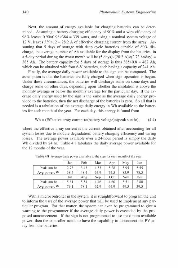
Photovoltaic Systems Engineering140
Next, the amount of energy available for charging batteries can be deter-mined. Assuming a battery-charging efficiency of 90% and a wire efficiency of98% leaves 0.90×0.98×384 = 339 watts, and using a nominal system voltage of12 V, leaves 339÷12 = 28.2 A of effective charging current from the array. As-suming that 5 days of storage with deep cycle batteries capable of 80% dis-charge, the average number of Ah available for the display from the batteries ina 5-day period during the worst month will be (5 days)×(28.2 A)×(2.73 hr/day) =385 Ah. The battery capacity for 5 days of storage is thus 385÷0.8 = 482 Ah,which can be obtained with four 6-V batteries, each having a capacity of 241 Ah.
Finally, the average daily power available to the sign can be computed. Theassumption is that the batteries are fully charged when sign operation is begun.Under these circumstances, the batteries will discharge some on some days andcharge some on other days, depending upon whether the insolation is above themonthly average or below the monthly average for the particular day. If the av-erage daily energy used by the sign is the same as the average daily energy pro-vided to the batteries, then the net discharge of the batteries is zero. So all that isneeded is a tabulation of the average daily energy in Wh available to the batter-ies for each month of the year. For each day, this energy is found from
Wh = (Effective array current)×(battery voltage)×(peak sun hr), (4.4)
where the effective array current is the current obtained after accounting for allsystem losses due to module degradation, battery charging efficiency and wiringlosses. The average power available over a 24-hour period is simply the dailyWh divided by 24 hr. Table 4.8 tabulates the daily average power available forthe 12 months of the year.
Table 4.8 Average daily power available to the sign for each month of the year.
Jan Feb Mar Apr May JunPeak sun hr 2.73 3.43 4.53 5.28 5.95 5.55
Avg power, W 38.5 48.4 63.9 74.5 83.9 78.3Jul Aug Sep Oct Nov Dec
Peak sun hr 5.61 5.54 4.46 4.60 3.51 2.80Avg power, W 79.1 78.1 62.9 64.9 49.5 39.5
With a microcontroller in the system, it is straightforward to program the unitto inform the user of the average power that will be used to implement any par-ticular program. For that matter, the system can even be programmed to give awarning to the programmer if the average daily power is exceeded by the pro-posed announcement. If the sign is not programmed to use maximum availablepower, then the controller needs to have the capability to disconnect the PV ar-ray from the batteries.
Chapter 4 PV System Examples 141
Problems
4.1 For the fan example, indicate applications for which it would be desirableto have an oversized PV module and indicate when it would be satisfactoryto have a smaller module that would produce a significantly lower fanspeed at lower light levels. Can you envision an application for which useof a MPT would be advantageous?
4.2 For the alternate pumping example in Section 4.3.3, show that the valuesobtained for n and for V2 are correct under the assumptions made in theexample.
4.3 How much power could be recovered at low light levels by using an MPTon the fan of the first example in the text, assuming the MPT to be 90% ef-ficient? Estimate the additional maximum power output that would be re-quired of a PV array that would produce the same low-light-level power asthe system with the MPT. If the additional PV cost $5/watt, how muchcould you spend on the MPT to produce the same effect?
4.4 Prove that equations 4.1a and 4.1b are correct.
4.5 Determine the lamp wattage required to obtain an illumination level of 50f-c over a 100 ft2 area if a fixture is used with a CU of 0.75 and 80% of theavailable light reaches the work surface, the rest being absorbed by wallsand other items in the space. Assume a luminous efficacy of 70 lu-mens/watt.
4.6 If the lamp of Problem 4.5 is on for an average of 6 hours per day, and ifpeak sun hours average 6 hours per day,a. Determine the power output required for a PV array that would power
the lamp, assuming 10% degradation of the PV array.b. Determine a general expression for PV array power as a function of
lamp operating time, assuming full utilization of the PV output.
4.7 For the remote cabin of Section 4.5, sketch the state of charge of the bat-teries for a 7-day period, assuming the batteries begin on Monday morning80% discharged and assuming the following conditions:a. three day occupancy over a weekend and average peak sun every dayb. two day occupancy over a weekend and average peak sun every dayc. three day occupancy over a weekend and 3 hours peak sun on Monday,
6 on Tuesday, 2 on Wednesday, 5 on Thursday, 6 on Friday, 2 on Sat-urday and 5 on Sunday.
4.8 For the hybrid system of Section 4.6:a. Explain why the system will have 18.8 days of leeway for refueling re-
sulting from the choice of a 1200 gal fuel tank.

Photovoltaic Systems Engineering142
b. Suggest two good times during the year for refueling. Explain your rea-sons, keeping in mind that not much fuel is used in the summer.
4.9 For the hybrid system of Section 4.6, determine the type and amount ofannual maintenance that will be required for the generator if it is aa. 3600 rpm gasoline generatorb. 1800 rpm gasoline generatorc. 1800 rpm diesel generator
4.10 For the hybrid system of Section 4.6, determine the wire size needed tocarry the battery charging current from the battery charger to the batteries,assuming voltage drop is not a problem. The wire must be able to carry125% of the charging current. Parallel conductors are allowed, providedthat they are of the same size.
4.11 Sketch the battery system of Section 4.6 and recommend methods of wiringthat will balance the current in each of the parallel sets of batteries. Keepin mind that the cell voltages of all batteries may not be exactly equal.Then make a search for batteries with higher Ah ratings to determinewhether fewer than 15 parallel battery sets are possible.
4.12 Assuming voltage drop in wiring not to be a problem, determine the wiresizes needed to carry the currents on the dc and ac sides of the inverter ofthe utility interactive example of Section 4.7. You might find Table 3.7 tobe useful. Note that the source circuit wiring must be capable of carrying156% of ISC of the array, and the inverter output circuit wiring must be ca-pable of carrying 125% of the rated output current of the inverter.
4.13 For a soil with a resistivity of 12,000 Ω-cm, and a cathode that requires200 mA of current for protection, configure an anode system that will al-low the use of a 12 volt system. Then select a battery to provide 5 days ofstorage and a module(s) to supply the system energy needs if theminimum insolation is 3 hr/day.
4.14 For a soil with resistivity of 20,000 Ω-cm, and a cathode that requires 500mA of current for protection, configure an anode system that will allow theuse of a 12-volt system. Then select a battery to provide 5 days of storageand a module(s) to supply the system energy needs for minimum peaksun of 2.5 hr/day.
4.15 To test the soil resistivity after a large steel tank has been buried, a 6-ft-long, 4-in-diameter anode is buried about 40 ft from the tank. When a 12V battery is connected between the anode and the tank, a current of 0.5 Aflows. What is the resistivity of the soil?

Chapter 4 PV System Examples 143
4.16 The highway information sign is to be designed for use in Miami, FL, usingthe same PV panels. The sign still requires 5 days of autonomy underworst case sun conditions, so the battery requirements will need to be re-calculated. Then tabulate the average daily power available to the sign foreach of the 12 months of the year.
4.17 Redo the highway information sign example for use in Phoenix, AZ, againcalculating the battery requirements and then showing the monthly averagedaily power availability.
4.18 For the highway sign of Section 4.9, determine the Ah rating of batteriesthat will provide 5 days of backup power for the month with the highestaverage daily sun hours.
4.19 How many days of storage will the batteries of the highway sign exampleof Section 4.9 provide at summer average daily power levels?
References
[1] 1997-98 Design Guide & Catalog, Alternative Energy Engineering, Redway, CA,1997.
[2] Lighting Handbook: Reference and Application, 8th Ed., Illuminating EngineeringSociety of North America, New York, 1993.
[3] IES Lighting Handbook, Illuminating Engineering Society of North America, NewYork, 1984.
[4] 9200 Lamp Catalog, 22nd Ed., GE Lighting, General Electric Co., 1995. [5] Lamp Specification and Application Guide, Philips Lighting Co., Somerset , NJ,
1999. [6] www.cetsolar.com for information on LED arrays. [7] www.aseamerica.com for information on ASE PV modules. [8] www.dsireusa.org/summarytables for information on state renewable programs. [9] Stand-Alone Photovoltaic Systems: A Handbook of Recommended Design Practices,
Sandia National Laboratories, Albuquerque, NM, 1995.
Suggested Reading
Blier, F., Fan Handbook: Selection, Application and Design, McGraw-Hill, NewYork, 1998.
NFPA 70 National Electrical Code, 1999 Edition, National Fire Protection Asso-ciation, Quincy, MA, 1998.
Roberson, J. A. and Crowe, C. T., Engineering Fluid Mechanics, 3rd Ed., HoughtonMifflin, Boston, MA, 1985.
www.astropower.com for information on AstroPower modules.www.batteries4everything.com for information on a variety of batteries.www.fsec.ucf.edu for a wide range of information and links to other PV products
and systems.www.sma-america.com for information on Sunny Boy inverters.www.xantrex.com for information on Xantrex inverters.

145
Chapter 5COST CONSIDERATIONS
5.1 Introduction
The costs of a PV system include acquisition costs, operating costs, mainte-nance costs and replacement costs. At the end of the life of a system, the systemmay have a salvage value or it may have a decommissioning cost. This chapterintroduces the method of life cycle costing, which accounts for all costs associ-ated with a system over its lifetime, taking into account the time value of money.Life cycle costing is used in the design of the PV system that will cost the leastamount over its lifetime. Life cycle costing, in general, constitutes a sensiblemeans for evaluating any purchase options.
If it is necessary to borrow money to purchase an item, the cost of the loanmay also need to be incorporated into the total cost of a system.
This chapter also introduces the concept of externalities. Externalities arecosts that are not normally directly associated with an item. For example, it isgenerally agreed that acid rain can be caused by sulfur emissions from smoke-stacks. It is also generally agreed that acid rain can cause damage to buildingsand lakes. Yet, the cost of these damages is generally not paid for directly bythe entity that generates the emissions. Externalities will be considered in moredetail in Chapter 9.
5.2 Life Cycle Costing
5.2.1 The Time Value of Money
The life cycle cost of an item consists of the total cost of owning and operat-ing an item over its lifetime. Some costs involved in the owning and operatingof an item are incurred at the time of acquisition, and other costs are incurred atlater times. In order to compare two similar items, which may have differentcosts at different times, it is convenient to refer all costs to the time of acquisi-tion. For example, one refrigerator may be initially less expensive than another,but it may require more electrical energy and more repairs over its lifetime. Theadditional costs of electrical energy and repairs may more than offset the loweracquisition cost.
Two phenomena affect the value of money over time. The inflation rate, i,is a measure of the decline in value of money. For example, if the inflation rateis 3% per year, then an item will cost 3% more next year. Since it takes moremoney to purchase the same thing, the value of the unit of currency, in effect, isdecreased. Note that the inflation rate for any item need not necessarily followthe general inflation rate. Recently health care costs have exceeded the generalinflation rate in the U.S., while the cost of most electronic goods have fallen farbelow the general inflation rate.
Photovoltaic Systems Engineering146
The discount rate, d, relates to the amount of interest that can be earned onprincipal that is saved. If money is invested in an account that has a positiveinterest rate, the principal will increase from year to year. The real challenge,then, in investing money, is to invest at a discount rate that is greater than theinflation rate.
As an example, assume an initial amount of money is invested at a rate of100d% per year, where d is the percentage rate expressed as a fraction. After nyears, the value of the investment will be
( ) no d1N)n(N += . (5.1)
However, in terms of the purchasing power of this investment, N(n) dollars willnot purchase the same amount as this amount of money would have purchased atthe time the investment was made. In order to account for inflation, note that ifthe cost of an item at the time the investment was made is Co, then the cost ofthe item after n years if the inflation rate is 100i% per year, will be
.)i1(C)n(C no += (5.2)
One might argue that if the cost of an item increases at a rate that exceeds therate at which the value of saved money increases, that the item should be pur-chased right away. Similarly, if the cost of the item increases more slowly, or,perhaps, actually decreases over time, then one should wait before making thepurchase, since the cost will be less at a later time. The disadvantage of this pur-chasing algorithm, of course, is that the item to be purchased will not be avail-able for use until it is purchased. Hence, the new computer that becomes lessand less expensive while the invested money continues to increase, is not avail-able for computing when it should be purchased. In other words, economics maynot be the only consideration in making a purchase. Sometimes people buythings simply because they want them.
It is important to remember that choosing values for d and i is tantamount topredicting the future, since d and i fluctuate over time. Depending upon thesaving mechanism, the rate of return may be fixed or may be variable. Inflationis, at best, unpredictable.
Figure 5.1 shows how the consumer price index, as a measure of inflation,the Dow Jones industrial average, as one possible measure of d, and the govern-ment prime lending rate, as a measure of the minimum borrowing interest rate,have varied over the period between 1980 and 2002. It is interesting to note howthe prime lending rate is adjusted with the intent of either controlling inflation bydiscouraging borrowing or stimulating the economy by encouraging borrowing.The high prime lending rate in the early 1980s reflects the attempt to controlhigh inflation in the late 1970s resulting from significant increases in energyprices during this period. The low rate in 2002 reflects the attempt to stimulatethe economy and bring about a recovery of the stock market.
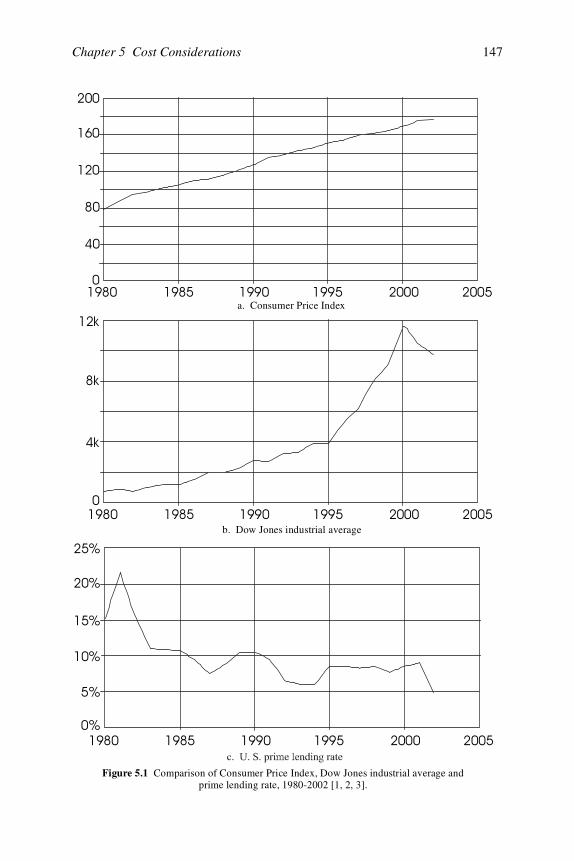
Chapter 5 Cost Considerations 147
a. Consumer Price Index
b. Dow Jones industrial average
Figure 5.1 Comparison of Consumer Price Index, Dow Jones industrial average and prime lending rate, 1980-2002 [1, 2, 3].
Photovoltaic Systems Engineering148
5.2.2 Present Worth Factors and Present Worth
If Co = No, the ratio of C(n) to N(n) becomes a dimensionless quantity, Pr,which represents the present worth factor of an item that will be purchased nyears later, and is given by
n
d1i1
Pr
++= . (5.3)
The present worth of an item is defined as the amount of money that wouldneed to be invested at the present time with a return of 100d% in order to be ableto purchase the item at a future time, assuming an inflation rate of 100i%.Hence, for the item to be purchased n years later, the present worth is given by
PW = (Pr)Co . (5.4)
Sometimes it is necessary to determine the present worth of a recurring ex-pense, such as fuel cost. Since recurring expenses can be broken down into aseries of individual expenses at later times, it is possible to determine the presentworth of a recurring expense by simply summing up the present worth of each ofthe series. For example, suppose a commodity such as diesel fuel is to be usedover the lifetime of a diesel generator. It is desired to determine how muchmoney must be invested at present at an annual interest rate of 100d%, underconditions of 100i% annual inflation in order to purchase fuel for n years. If thefirst year’s supply of fuel is purchased at the time the system is put into opera-tion, and each successive year’s fuel supply is purchased at the beginning of theyear, the present worth of the fuel acquisitions will be
PW = 1n
o
3
o
2
ooo d1i1
C...d1i1
Cd1i1
Cd1i1
CC−
++++
+++
+++
+++ . (5.5)
Letting x =
++
d1i1
, (5.5) becomes
PW = )x...xx1(C 1n2o
−++++ . (5.5a)
This expression can be simplified by observing that
∑∞
=
=++++=−
0i
i32 x...xxx1x1
1. (5.6)
Now, the cumulative present worth factor can be defined as
Chapter 5 Cost Considerations 149
Pa = PW/Co = ∑∑∞
=
∞
=
−−
=−−
0i
in
ni
i xxx1
1x
x11
,
or, finally,
Pa = x1
x1 n
−−
. (5.7)
It is important to recognize that (5.7) is based on the assumption that the firstyear’s supply is purchased at the beginning of the year at a time when the fuel isat its present value. The fuel is then purchased annually with the last purchaseoccurring one year before the system lifetime has expired. In other words, thereare n purchases of fuel, each at the beginning of the nth year.
If the recurring purchase does not begin until the end of the first year, and ifthe last purchase occurs at the end of the useful life of the system, there will stillbe n purchases, but, using x again, the cumulative present worth factor be-comes
Pa1 = n32 x...xxx ++++
)x...xx1(x 1n2 −++++= = xPa . (5.8)
Since x will typically be in the range 0.95 < x < 1.05, and since determination ofi and d are at best, good guesses, and since it would be unusual to purchase anentire year’s supply of many things all at once at the beginning of the year or atthe end of the year, either (5.7) or (5.8) will provide a good estimate of the pres-ent worth of a cumulative expenditure. Often the values for Pr and for Pa aretabulated. Since most engineers have programmable calculators and computers,there is little point in repeating tabulated values for these expressions. Once thevalues for the variables have been decided upon, the present worth of quantitiescan be calculated. For that matter, if an engineer wanted to assume differentvalues for d and i for different years, the same methodology could be used todetermine the present worth of a quantity.
5.2.3 Life Cycle Cost
Once the PW is known for all cost categories relating to the purchase, main-tenance and operation of an item, the life cycle cost (LCC) is defined as the sumof the PWs of all the components. The life cycle cost may contain elementspertaining to original purchase price, replacement prices of components, mainte-nance costs, fuel and/or operation costs, and salvage costs or salvage revenues.Calculating the LCC of an item provides important information for use in theprocess of deciding which choice is the most economical. The following exam-ple demonstrates the use of LCC.
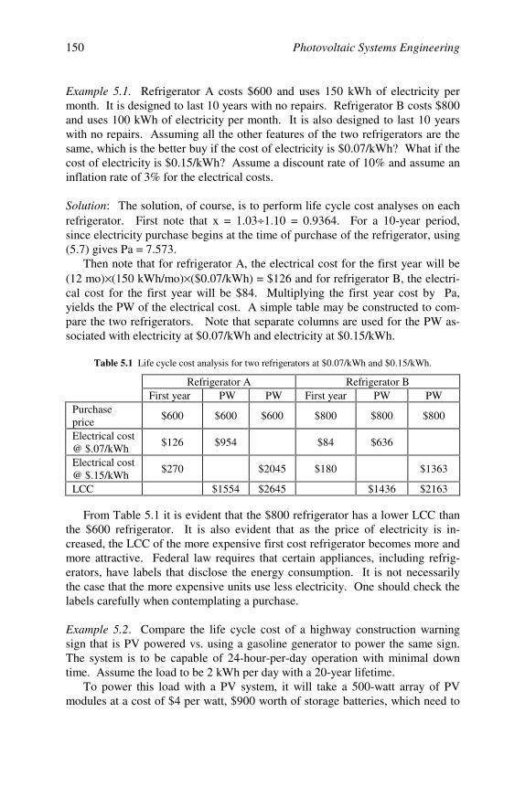
Photovoltaic Systems Engineering150
Example 5.1. Refrigerator A costs $600 and uses 150 kWh of electricity permonth. It is designed to last 10 years with no repairs. Refrigerator B costs $800and uses 100 kWh of electricity per month. It is also designed to last 10 yearswith no repairs. Assuming all the other features of the two refrigerators are thesame, which is the better buy if the cost of electricity is $0.07/kWh? What if thecost of electricity is $0.15/kWh? Assume a discount rate of 10% and assume aninflation rate of 3% for the electrical costs.
Solution: The solution, of course, is to perform life cycle cost analyses on eachrefrigerator. First note that x = 1.03 ÷ 1.10 = 0.9364. For a 10-year period,since electricity purchase begins at the time of purchase of the refrigerator, using(5.7) gives Pa = 7.573.
Then note that for refrigerator A, the electrical cost for the first year will be(12 mo) × (150 kWh/mo) × ($0.07/kWh) = $126 and for refrigerator B, the electri-cal cost for the first year will be $84. Multiplying the first year cost by Pa,yields the PW of the electrical cost. A simple table may be constructed to com-pare the two refrigerators. Note that separate columns are used for the PW as-sociated with electricity at $0.07/kWh and electricity at $0.15/kWh.
Table 5.1 Life cycle cost analysis for two refrigerators at $0.07/kWh and $0.15/kWh.
Refrigerator A Refrigerator BFirst year PW PW First year PW PW
Purchaseprice
$600 $600 $600 $800 $800 $800
Electrical cost@ $.07/kWh
$126 $954 $84 $636
Electrical cost@ $.15/kWh
$270 $2045 $180 $1363
LCC $1554 $2645 $1436 $2163
From Table 5.1 it is evident that the $800 refrigerator has a lower LCC thanthe $600 refrigerator. It is also evident that as the price of electricity is in-creased, the LCC of the more expensive first cost refrigerator becomes more andmore attractive. Federal law requires that certain appliances, including refrig-erators, have labels that disclose the energy consumption. It is not necessarilythe case that the more expensive units use less electricity. One should check thelabels carefully when contemplating a purchase.
Example 5.2. Compare the life cycle cost of a highway construction warningsign that is PV powered vs. using a gasoline generator to power the same sign.The system is to be capable of 24-hour-per-day operation with minimal downtime. Assume the load to be 2 kWh per day with a 20-year lifetime.
To power this load with a PV system, it will take a 500-watt array of PVmodules at a cost of $4 per watt, $900 worth of storage batteries, which need to
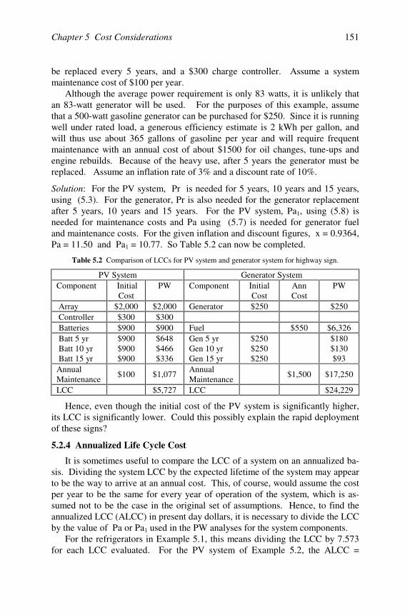
Chapter 5 Cost Considerations 151
be replaced every 5 years, and a $300 charge controller. Assume a systemmaintenance cost of $100 per year.
Although the average power requirement is only 83 watts, it is unlikely thatan 83-watt generator will be used. For the purposes of this example, assumethat a 500-watt gasoline generator can be purchased for $250. Since it is runningwell under rated load, a generous efficiency estimate is 2 kWh per gallon, andwill thus use about 365 gallons of gasoline per year and will require frequentmaintenance with an annual cost of about $1500 for oil changes, tune-ups andengine rebuilds. Because of the heavy use, after 5 years the generator must bereplaced. Assume an inflation rate of 3% and a discount rate of 10%.
Solution: For the PV system, Pr is needed for 5 years, 10 years and 15 years,using (5.3). For the generator, Pr is also needed for the generator replacementafter 5 years, 10 years and 15 years. For the PV system, Pa1, using (5.8) isneeded for maintenance costs and Pa using (5.7) is needed for generator fueland maintenance costs. For the given inflation and discount figures, x = 0.9364,Pa = 11.50 and Pa1 = 10.77. So Table 5.2 can now be completed.
Table 5.2 Comparison of LCCs for PV system and generator system for highway sign.
PV System Generator SystemComponent Initial
CostPW Component Initial
CostAnnCost
PW
Array $2,000 $2,000 Generator $250 $250 Controller $300 $300 Batteries $900 $900 Fuel $550 $6,326 Batt 5 yr Batt 10 yr Batt 15 yr
$900$900$900
$648$466$336
Gen 5 yrGen 10 yrGen 15 yr
$250$250$250
$180$130$93
AnnualMaintenance
$100 $1,077AnnualMaintenance
$1,500 $17,250
LCC $5,727 LCC $24,229
Hence, even though the initial cost of the PV system is significantly higher,its LCC is significantly lower. Could this possibly explain the rapid deploymentof these signs?
5.2.4 Annualized Life Cycle Cost
It is sometimes useful to compare the LCC of a system on an annualized ba-sis. Dividing the system LCC by the expected lifetime of the system may appearto be the way to arrive at an annual cost. This, of course, would assume the costper year to be the same for every year of operation of the system, which is as-sumed not to be the case in the original set of assumptions. Hence, to find theannualized LCC (ALCC) in present day dollars, it is necessary to divide the LCCby the value of Pa or Pa1 used in the PW analyses for the system components.
For the refrigerators in Example 5.1, this means dividing the LCC by 7.573for each LCC evaluated. For the PV system of Example 5.2, the ALCC =
Photovoltaic Systems Engineering152
$5727 ÷ 10.77 = $532, and for the gasoline generator system of Example 5.2, theALCC = $24,229 ÷ 11.5 = $2,107.
5.2.5 Unit Electrical Cost
One especially valuable use of the ALCC is to determine the unit cost ofelectricity produced by an electrical generating system. Obviously if the elec-tricity is to be sold, it is necessary to know the price for which it should be soldto either earn a profit or to at least know how much will be lost in the process.Once the ALCC is known, the unit electrical cost is simply the ALCC divided bythe annual electrical production. If the annual electrical production is measuredin kWh, then the unit electrical cost will be measured in $/ kWh.
For the PV system of Example 5.2, the unit electrical cost is ALCC/kWh =$532 ÷ 730 = $0.729/kWh. For the gasoline generator system, the unit electricalcost is $2107 ÷ 730 = $2.89/kWh. Clearly, both of these costs far exceed thecost of utility-generated electricity, but since this is a portable application, wherethe sign is moved around from day to day, the cost of hooking up and discon-necting the system from utility power is impractical, at best.
5.3 Borrowing Money
5.3.1 Introduction
Sometimes the desire to own something causes the potential owner to realizethat money does not grow on trees. While some money comes from paychecks,usually larger sums of money come from borrowing from banks or other lendinginstitutions. The question at this point for the engineer-turned-economist iswhether borrowed money is any different from paycheck money or money froma savings account, a mattress or other form of liquid asset. For example, if themoney to purchase one of the refrigerators of Example 5.1 had to be borrowedrather than taken from a wallet, would that affect the LCC of the refrigerator?
Once again, tables are readily available for looking up the annual paymentson a loan of Co dollars taken out at 100i% annual interest over a period of nyears. For that matter, it is possible to purchase a calculator that will automati-cally yield the answer when it has been given the terms of the loan. An engineer,of course, will want to know how the numbers are obtained.
5.3.2 Determination of Annual Payments on Borrowed Money
To satisfy this curiosity, consider Table 5.3, representing the principal, inter-est, total payments and principal balance at the end of the kth year for repaymentof an n-year loan at 100i% annual interest, where Co represents the amount bor-rowed. Note that during any of the years, it is not yet known how much will bepaid on the principal in order to repay all of the principal in n years. The chal-
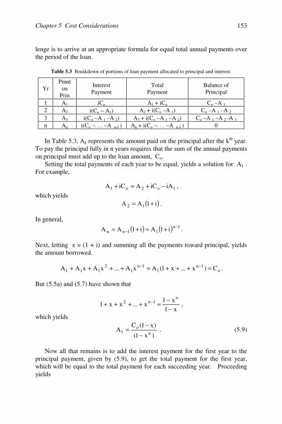
Chapter 5 Cost Considerations 153
lenge is to arrive at an appropriate formula for equal total annual payments overthe period of the loan.
Table 5.3 Breakdown of portions of loan payment allocated to principal and interest.
YrPmnt
onPrin
InterestPayment
TotalPayment
Balance ofPrincipal
1 A1 iCo A1 + iCo Co – A 1
2 A2 i(Co − A1) A2 + i(Co – A 1) Co – A 1 – A 2
3 A3 i(Co – A 1 – A 2) A3 + i(Co – A 1 – A 2) Co – A 1 – A 2 –A 3
n An i(Co – . . . – A n–1 ) An + i(Co – . . . – A n–1 ) 0
In Table 5.3, Ak represents the amount paid on the principal after the kth year.To pay the principal fully in n years requires that the sum of the annual paymentson principal must add up to the loan amount, Co.
Setting the total payments of each year to be equal, yields a solution for A1 .For example,
1o2o1 iAiCAiCA −+=+ ,
which yields( )i1AA 12 += .
In general,
( ) ( ) 1n11nn i1Ai1AA −
− +=+= .
Next, letting x = (1 + i) and summing all the payments toward principal, yieldsthe amount borrowed.
o1n
11n
12
111 C)x...x1(AxA...xAxAA =+++=++++ −− .
But (5.5a) and (5.7) have shown that
x1x1
x...xx1n
1n2
−−=++++ − ,
which yields
)x1(
)x1(CA
no
1 −−
= . (5.9)
Now all that remains is to add the interest payment for the first year to theprincipal payment, given by (5.9), to get the total payment for the first year,which will be equal to the total payment for each succeeding year. Proceedingyields
Photovoltaic Systems Engineering154
ANN PMT =
+
−+=+
−−
i1)i1(
iCiC
)x1(
)x1(Cnoon
o .
Simplifying this result yields, finally,
ANN PMT =
−++
1)i1(
)i1(iC
n
n
o . (5.10)
Usually payments are made monthly rather than annually. In this case, oneneed only note that rather than n payments, there will be 12n payments, and themonthly interest rate will simply be the annual rate divided by 12. Doing soconverts (5.10) into an equation for monthly payments. Obviously, if one wantsto split hairs even more finely, (5.10) could be modified for weekly, daily orhourly payments. Equation (5.10) is also an equation that might be convenientlytabulated for various values of i and n, but again it is left to the reader to useeither a computer or a programmable calculator to generate the numbers thatapply to the problem at hand.
5.3.3 The Effect of Borrowing on Life Cycle Cost
Depending on the nature of a purchase, it is interesting to compare whetherthe cost of borrowing money will render the purchase undesirable. For example,if money is borrowed to purchase something that will provide a return on theinvestment, it may make economic sense to borrow the money. This is the stan-dard criterion for commercial loans. The better the return, the better the reasonto borrow the money. But what if it is necessary to borrow the money for theinitial cost of a system that does not have an obvious return on investment?Does it make sense to borrow for something having a greater first cost if it re-sults in higher loan repayment costs? Although there are several ways to evalu-ate the worthiness of a purchase, once again, people sometimes borrow money topurchase things that do not have a measurable monetary return on investment,such as automobiles, simply because they want them.
As a simple example, suppose it is possible to spend $2000 on a mainte-nance-free system that will last for 25 years and will reduce an electric bill by acertain amount per year. The exact system might be insulation, good windows, asolar water heater, or any number of energy efficiency measures. Suppose alsothat money is borrowed to purchase the system and the period of the loan is 25years. This would be the case if the system is purchased for a dwelling at thetime of construction and the item is included in the 25-year mortgage. If themortgage rate is 9%, then (5.10) shows the additional annual mortgage paymentswould be $203.61. If the annual savings on the electric bill exceed $203.61,then it is worth borrowing the money.
Chapter 5 Cost Considerations 155
One should note, however, that the additional $203.61 mortgage paymentwill be constant over the life of the loan. In an inflationary environment, thismeans that even though the electric bill savings may not be $203.61 the firstyear, after a certain number of years, the annual savings may well exceed$203.61, making the investment worth considering.
What if the money is not borrowed? What if the $2000 is at hand and avail-able for investing? What would be the return on investment if it is spent on oneof the items of the previous example? The simple answer would say the return isequal to the resulting savings less the resulting operating or maintenance costs.This works fine for the first year, but for successive years to yield a more preciseestimate, the time value of money must be taken into account. Assuming thevalue of the quantity saved increases at the inflation rate, i, and the discount rateis d, the present worth of the savings accrued over n years will be given by (5.5).As a result, the PW of the annual savings over n years is given by (5.7). Hence,(5.7) can be applicable in either an expenditure mode or in a savings mode. Byconverting costs and savings to LCC, it is easy to compare savings with costs todetermine whether to make the purchase.
Assuming that a system must be acquired to do something, and assuming thatthe system with the least LCC has been identified, it is simply a matter of decid-ing whether to borrow money or to use money on hand, if, indeed, the money ison hand. If the money is not on hand, then the only option is to borrow. If themoney is on hand, then the criteria is whether the lending rate is less than ormore than the discount rate. If money can be borrowed at a rate less than what itcan earn, then it makes sense to borrow for the acquisition and to invest themoney that might have been used for the purchase. This is a choice often madeby the buyer of a new automobile. Should the savings account be used or shouldthe money be borrowed? The answer depends on the relative interest on savingsvs. the interest on the loan.
5.4 Externalities
5.4.1 Introduction
What happens if something owned and operated by one entity causes damageto something owned by another entity? A quick response would be that the en-tity causing the damage would be liable, and that the cost of repair of the dam-aged property should be the responsibility of the entity doing the damage. Theproblem is complicated in many instances, however, when more than one entityis responsible for creating the cause of the damage, and when more than oneentity suffers damage as a result of the cause. And it gets even more murkywhen debate ensues over whether the alleged cause is really the cause. Classicexamples of such situations are the link between smoking and cancer and the linkbetween burning of fossil fuels, acid rain and global warming.
Much debate has taken place regarding the liability of tobacco companies foralleged firsthand, smoke-induced cancer and even regarding the alleged inci-

Photovoltaic Systems Engineering156
dence of secondhand, smoke-induced cancer. Until recent large judgmentsagainst the tobacco industry, the cost of producing cigarettes did not include acomponent to underwrite the cost of paying the judgments. Yet, it has been ar-gued that tobacco is the cause of billions of dollars in medical bills, none ofwhich have been paid out of tobacco revenues. Thus, in the past, the medicalbills incurred by those exposed to tobacco smoke have been treated as external-ities by the tobacco industry, while in the present, these bills have become directcost components of doing business.
There is now reasonable agreement that one cause of acid rain is the burningof fuel that contains sulfur, such as petroleum or coal. As a result, many powerplants are now equipped with elaborate scrubbers that remove sulfur and otherpollutants from smokestack emissions.
Although a price per pound has not been established for sulfur emissions, theEnvironmental Protection Agency has established limits on the amounts of vari-ous pollutants that may be contained in smokestack emissions. Limits also existfor regions, so that if a region has met its limit, then no further burning may takeplace unless one of the burners can be made cleaner. In some cases, when acompany has not reached its emission limit, the company will sell or trade theremaining allowed emissions with another burner. As a result, monetary value isevolving for certain emissions, albeit in a bit of a roundabout way. The mone-tary value, however, does not relate directly to the damage done in either theform of acid rain damage or the cost of respiratory diseases. The cost of scrub-bers, however, appears as a system cost during the LCC process.
Another factor that needs consideration in establishing cost is the effect ofvarious forms of subsidies. Some subsidies may enter the picture as direct costs,while others may appear as externalities.
5.4.2 Subsidies
When performing an LCC, sometimes the cost of a component, a fuel or theoperation of a system may be affected by a subsidy or subsidies. For example,the cost of military presence in a region to ensure the steady flow of a fuel fromthe region is never included in the selling price of the product. Mineral deple-tion allowances, however, can be factored into the selling price of a product. Inother cases, governments have been known to offer price supports in order toensure competitive prices in a world market. Tariffs, in effect, are a form ofsubsidy, since they ensure that domestic production will be sold at a profit, thusnot competing directly with less costly products from outside a country.
Green pricing is a form of subsidy for the acquisition of clean energysources. An example is when the customers of a utility express a willingness topay extra every month to ensure that a part of their energy mix comes from re-newable sources, such as photovoltaics.
Subsidies in the form of tax breaks tend to come and go on a year-by-yearbasis. For a few years during the 1970s, homeowners could deduct a fraction of
Chapter 5 Cost Considerations 157
the cost of a domestic solar hot water system from their federal income tax.Some states initiated grant programs to encourage homeowners to install solarsystems and some utilities established rebate programs for part of the cost ofinstalling various energy conservation measures, such as more efficient air con-ditioning or attic insulation. Recently, several states have created buy-downprograms in which rebates are offered toward the installation of PV systems.
The argument is often set forth that all competing interests must compete ona level playing field. The meaning is simply that with so many subsidies, someof which are obvious and others of which are hidden, it is difficult for two com-peting interests to engage in fair competition. This is true in many industries andparticularly in the energy industry.
The reader is thus reminded that no economic analysis or comparison iscomplete until all forms of subsidy have been considered.
5.4.3 Externalities and Photovoltaics
The cost of an electrical generation source often excludes externalities. Sub-sequently, if a source is cleaner from an environmental viewpoint but has ahigher LCC based on parameters considered, that source may not be chosen. Aproper treatment of externalities includes not only the operating externalities, butthe externalities associated with the construction and salvage or decommission-ing of the facility. In both categories, photovoltaics show significant advantagesover nonrenewable sources, as will be shown in Chapter 9.
Problems
5.1 Obtain the data for Consumer Price Index, Dow Jones industrial averageand prime lending rate from references 1-3. Plot the data and attempt to fitcurves to the data to show trends. For example, use Excel graphs withtrendlines, equations and R2 values added to show the “goodness of fit.”Compare the R2 values for linear, exponential and polynomial fits to yourcurves.
5.2 Determine the present electricity cost for which the $600 refrigerator ofExample 5.1 will have the same LCC as the $800 unit, assuming all otherparameters to be the same.
5.3 Next time you are in an appliance store, record the first cost and annualoperating costs of several refrigerators that are comparable. Then, makingreasonable assumptions about discount rates, inflation rates and appliancelifetimes, compare the LCCs of the units. You might want to ask a sales-
Photovoltaic Systems Engineering158
person for information on expected lifetime and repair costs of the units,including annual maintenance contracts.
5.4 Use (5.10) to compare 12 equal monthly payments to one annual paymentby modifying the equation to account for monthly interest rate vs. annualrate and monthly payments vs. annual payments. How does the sum of 12monthly payments compare with a single annual payment?
5.5 Rework Example 5.2 for a system that uses 4 kWh per day. This will re-quire double the PV array and double the batteries, as well as double thefuel. However, the cost of the generator will remain the same and the costof the maintenance will remain the same. You may also assume doublethe cost of the charge controller.
5.6 Calculate a set of reasonable conditions on interest rate, term of loan andcost per installed kW, for a PV system that generates power for an averageof 5 peak sun hours per day so the annual loan repayment can be recoveredif the value of the electricity generated is $0.10/kWh.
5.7 The value of electricity during utility peaking hours is $0.20/kWh and themoney for a utility interactive system with a 30-year expected lifetime canbe borrowed at an interest rate of 7%. Calculate the installed cost per kWfor the system that will result in annual loan payments equal to the value ofelectricity produced by the system if the electricity is produced during util-ity peak hours.
References
[1] ftp://ftp.bls.gov/pub/special.requests/cpi/cpiai.txt for Consumer Price Index data.[2] http://djindexes.com for Dow Jones industrial average data.[3] ftp://ftp.ny.frb.org/prime/Prime.txt for prime lending rate data.
Suggested Reading
42 U. S. C. § 7401 et. seq. (Clean Air Act).Markvart, T., Ed., Solar Electricity, John Wiley & Sons, Chichester, U.K., 1994.“National Appliance Energy Conservation Act of 1987” (PL 100–12 , March 17,
1987, 101 § 103).Stand-Alone Photovoltaic Systems: A Handbook of Recommended Design Prac-
tices, Sandia National Laboratories, Albuquerque, NM, 1995.

159
Chapter 6MECHANICAL CONSIDERATIONS
6.1 Introduction
Because the primary function of a photovoltaic system is to convert sunlightto electricity, often the role and importance of the mechanical aspects of thesystem are ignored. Most photovoltaic modules are designed to last 20 years orlonger. It is important that the other components in the system, including me-chanical components, have lifetimes equivalent to those for the PV modules. Itis also important that the mechanical design requirements of the system be con-sistent with the performance requirements as well as with the operational re-quirements of the system.
The mechanical design of photovoltaic systems cuts across a variety of dis-ciplines, most notably civil and mechanical engineering and, to a lesser extent,materials science, aeronautical engineering and architecture. More specifically,mechanical design involves:
• Determining the mechanical forces acting on the system.• Selecting, sizing and configuring structural members to support these
forces with an adequate margin of safety.• Selecting and configuring materials that will not degrade or deteriorate
unacceptably over the life of the system.• Locating, orienting and mounting the photovoltaic array so that it has
adequate access to the sun’s radiation , produces the required electricaloutput and operates over acceptable PV cell temperature ranges.
• Designing an array support structure that is aesthetically appropriate forthe site and application and provides for ease of installation and mainte-nance.
Each of these elements of the mechanical system will be discussed in moredetail throughout this chapter.
6.2 Important Properties of Materials
6.2.1 Introduction
Before discussing the mechanical design process, it is useful to review theproperties of materials, especially the non-photovoltaic materials that are im-portant components of photovoltaic systems. A fairly comprehensive list ofperformance properties of materials in response to various stimuli is presented inTable 6.1. However, for simplicity, the properties of materials can be groupedinto four general categories: electrical properties, mechanical properties, chemi-cal properties and thermal properties [2].
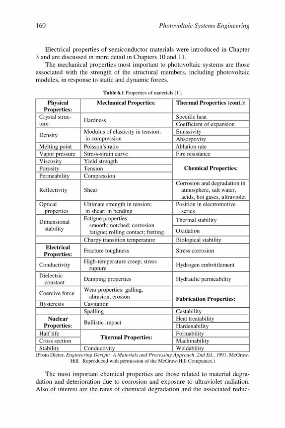
Photovoltaic Systems Engineering160
Electrical properties of semiconductor materials were introduced in Chapter3 and are discussed in more detail in Chapters 10 and 11.
The mechanical properties most important to photovoltaic systems are thoseassociated with the strength of the structural members, including photovoltaicmodules, in response to static and dynamic forces.
Table 6.1 Properties of materials [1].
PhysicalProperties:
Mechanical Properties: Thermal Properties (cont.):
Specific heatCrystal struc-ture
HardnessCoefficient of expansionEmissivity
DensityModulus of elasticity in tension; in compression Absorptivity
Melting point Poisson’s ratio Ablation rateVapor pressure Stress-strain curve Fire resistanceViscosity Yield strengthPorosity TensionPermeability Compression
Chemical Properties:
Reflectivity ShearCorrosion and degradation in
atmosphere, salt water,acids, hot gases, ultraviolet
Opticalproperties
Ultimate strength in tension; in shear; in bending
Position in electromotiveseries
Thermal stabilityDimensionalstability
Fatigue properties:smooth; notched; corrosionfatigue; rolling contact; fretting Oxidation
Charpy transition temperature Biological stabilityElectrical
Properties:Fracture toughness Stress corrosion
ConductivityHigh-temperature creep; stress
ruptureHydrogen embrittlement
Dielectricconstant
Damping properties Hydraulic permeability
Coercive forceWear properties: galling,
abrasion, erosionHysteresis Cavitation
Fabrication Properties:
Spalling CastabilityHeat treatabilityNuclear
Properties: Ballistic impactHardenability
Half life FormabilityCross section
Thermal Properties:Machinability
Stability Conductivity Weldability(From Dieter, Engineering Design: A Materials and Processing Approach, 2nd Ed., 1991, McGraw-
Hill. Reproduced with permission of the McGraw-Hill Companies.)
The most important chemical properties are those related to material degra-dation and deterioration due to corrosion and exposure to ultraviolet radiation.Also of interest are the rates of chemical degradation and the associated reduc-
Chapter 6 Mechanical Considerations 161
tion in lifetimes of various materials, such as those used for weather sealing andinsulation, that are caused by repeated exposure to high operating temperatures.
The thermal properties of most concern involve thermal expansion and con-traction and the resulting thermal stresses.
6.2.2 Mechanical Properties
The photovoltaic system, in particular the photovoltaic array and its struc-tural support members, is subjected to a variety of mechanical forces -- bothstatic and dynamic. These forces produce internal stresses and deformations.For common structural materials like steel and aluminum, there are limits tothese stresses and deformations that, if exceeded, may result in failure or irrepa-rable damage.
Stress is defined as force per unit area. Uniform normal stress occurs whena force P is normal to and distributed uniformly over a cross sectional area A. Itcan be calculated using the simple equation:
A
P
area
forceS == (6.1)
Why is the concept of stress important for the mechanical design of photo-voltaic systems? Because it is the ability of a structural member to withstandstresses (i.e., forces per unit area) that determines its strength. It is the engi-neer’s responsibility to first calculate or estimate the forces acting on the photo-voltaic system and then to select and size the structural support members suchthat the maximum stresses experienced are well below allowable limits.
The most common static forces acting on photovoltaic arrays and supportingstructures are due to the weight of the modules, mounting system and, in colderclimates, snow and ice. These forces produce a combination of uniform normal,shear and bending stresses that must not be overlooked in assessing the struc-tural integrity of the array and all of its supporting hardware. Heavy accumula-tions of snow and ice can produce high stress levels. However, in the over-whelming majority of cases, these types of static forces are not large enough toexceed the stress limits of the array structure.
In addition to static forces, the photovoltaic array and its support structurewill experience dynamic forces, most notably wind loads. Changes in wind di-rection and wind speed, including the rapid changes associated with gusting,complicate the job of the structural engineer. First, the changes in wind direc-tion often result in a structural member experiencing alternating periods of ten-sion and compression. Consequently, the structural members must be designednot only to withstand uniform tensile stress, but also not to buckle under com-pression. Second, the dynamic loads may give rise to a phenomenon known asfatigue failure. This occurs when the stresses in a structural member alternatebetween tension and compression over time and can occur at stress levels con-siderably below those that would produce a static stress failure. Fatigue firstmanifests itself as cracks on the surface of the structural member, often near a
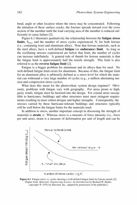
Photovoltaic Systems Engineering162
bend, angle or other location where the stress may be concentrated. Followingthe initiation of these surface cracks, the fracture spreads inward over the crosssection of the member until the load carrying area of the member is reduced suf-ficiently to cause failure [2].
Figure 6.1 illustrates qualitatively the relationship between the fatigue stresslimits, Smax, and the number of stress cycles experienced, N, for both ferrous(i.e., containing iron) and aluminum alloys. Note that ferrous materials, such asthe steel alloys, have a well-defined fatigue (or endurance) limit. As long asthe oscillating stresses experienced are below that limit, the number of cyclescan increase indefinitely. A general rule of thumb for ferrous materials is thatthe fatigue limit is approximately half the tensile strength. This limit is alsoreferred to as the reverse fatigue limit [2].
Fatigue is a bigger problem for aluminum and its alloys than for steel. Nowell-defined fatigue limit exists for aluminum. Because of this, the fatigue limitfor an aluminum alloy is arbitrarily defined as a stress level for which the mate-rial can withstand a very large number of cycles (e.g., a million alternating ten-sion and compression stress cycles).
What does this mean for the photovoltaic system design engineer? Obvi-ously, problems with fatigue vary with geography. For areas prone to high,gusty winds, fatigue must be factored into the design. For coastal areas suscep-tible to hurricanes, buildings and other structures must meet stringent require-ments resulting in more robust designs and higher strengths. Consequently, thestresses carried by these hurricane-tolerant buildings and structures typicallywill be well below the fatigue limits for the materials used.
In addition to stress, another important concept in discussing the strength ofmaterials is strain, ε . Whereas stress is a measure of force intensity (i.e., forceper unit area), strain is a measure of deformation per unit of length and can be
1XPEHURIVWUHVVF\FOHVORJ1
)DWLJXHVWUHVVOLPLWVORJ6
PD[
$OXPLQXPDQGDOOR\V
)HUURXVPDWHULDOVVWHHO
:HOOGHILQHGIDWLJXHOLPLW
Figure 6.1 Fatigue stress vs. cycles showing a well-defined fatigue limit for ferrous metals [2].(Figure from by Richard W. Hanks,
copyright 1970, by Harcourt, Inc., adapted by permission of the publisher.)Materials Engineering Science: An Introduction
C
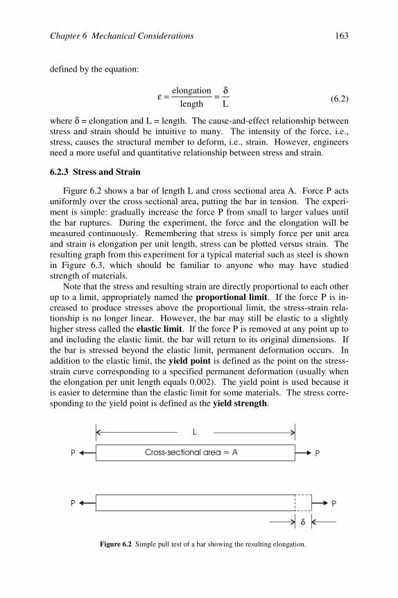
Chapter 6 Mechanical Considerations 163
defined by the equation:
(6.2)
where δ = elongation and L = length. The cause-and-effect relationship betweenstress and strain should be intuitive to many. The intensity of the force, i.e.,stress, causes the structural member to deform, i.e., strain. However, engineersneed a more useful and quantitative relationship between stress and strain.
6.2.3 Stress and Strain
Figure 6.2 shows a bar of length L and cross sectional area A. Force P actsuniformly over the cross sectional area, putting the bar in tension. The experi-ment is simple: gradually increase the force P from small to larger values untilthe bar ruptures. During the experiment, the force and the elongation will bemeasured continuously. Remembering that stress is simply force per unit areaand strain is elongation per unit length, stress can be plotted versus strain. Theresulting graph from this experiment for a typical material such as steel is shownin Figure 6.3, which should be familiar to anyone who may have studiedstrength of materials.
Note that the stress and resulting strain are directly proportional to each otherup to a limit, appropriately named the proportional limit. If the force P is in-creased to produce stresses above the proportional limit, the stress-strain rela-tionship is no longer linear. However, the bar may still be elastic to a slightlyhigher stress called the elastic limit. If the force P is removed at any point up toand including the elastic limit, the bar will return to its original dimensions. Ifthe bar is stressed beyond the elastic limit, permanent deformation occurs. Inaddition to the elastic limit, the yield point is defined as the point on the stress-strain curve corresponding to a specified permanent deformation (usually whenthe elongation per unit length equals 0.002). The yield point is used because itis easier to determine than the elastic limit for some materials. The stress corre-sponding to the yield point is defined as the yield strength.
Llength
elongation δ==ε
δ
Figure 6.2 Simple pull test of a bar showing the resulting elongation.
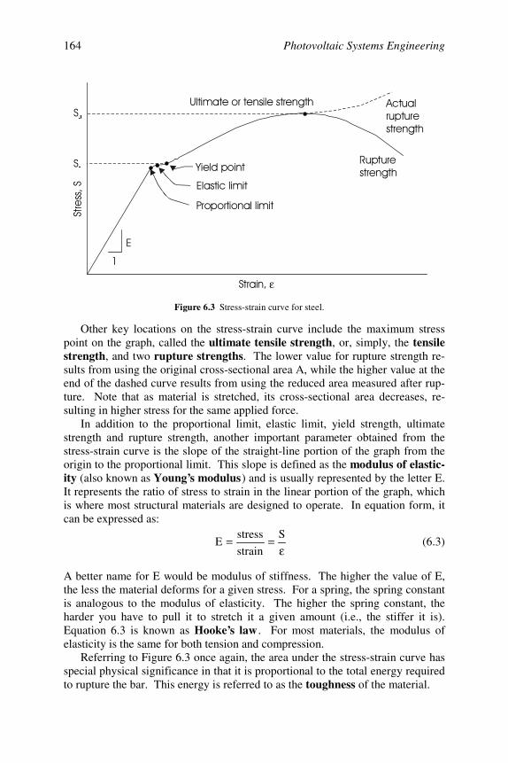
Photovoltaic Systems Engineering164
Other key locations on the stress-strain curve include the maximum stresspoint on the graph, called the ultimate tensile strength, or, simply, the tensilestrength, and two rupture strengths. The lower value for rupture strength re-sults from using the original cross-sectional area A, while the higher value at theend of the dashed curve results from using the reduced area measured after rup-ture. Note that as material is stretched, its cross-sectional area decreases, re-sulting in higher stress for the same applied force.
In addition to the proportional limit, elastic limit, yield strength, ultimatestrength and rupture strength, another important parameter obtained from thestress-strain curve is the slope of the straight-line portion of the graph from theorigin to the proportional limit. This slope is defined as the modulus of elastic-ity (also known as Young’s modulus) and is usually represented by the letter E.It represents the ratio of stress to strain in the linear portion of the graph, whichis where most structural materials are designed to operate. In equation form, itcan be expressed as:
ε== S
strain
stressE (6.3)
A better name for E would be modulus of stiffness. The higher the value of E,the less the material deforms for a given stress. For a spring, the spring constantis analogous to the modulus of elasticity. The higher the spring constant, theharder you have to pull it to stretch it a given amount (i.e., the stiffer it is).Equation 6.3 is known as Hooke’s law . For most materials, the modulus ofelasticity is the same for both tension and compression.
Referring to Figure 6.3 once again, the area under the stress-strain curve hasspecial physical significance in that it is proportional to the total energy requiredto rupture the bar. This energy is referred to as the toughness of the material.
ε
<
8
Figure 6.3 Stress-strain curve for steel.
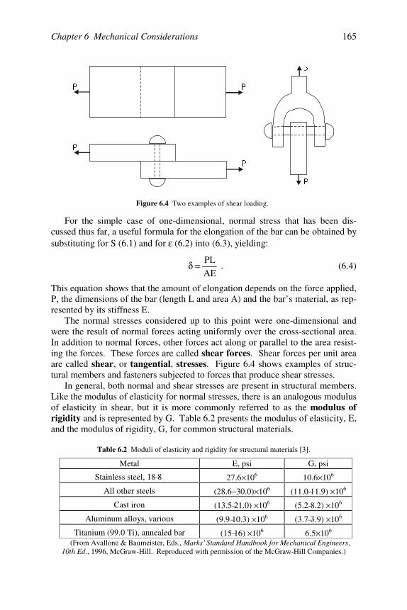
Chapter 6 Mechanical Considerations 165
For the simple case of one-dimensional, normal stress that has been dis-cussed thus far, a useful formula for the elongation of the bar can be obtained bysubstituting for S (6.1) and for ε (6.2) into (6.3), yielding:
AEPL=δ . (6.4)
This equation shows that the amount of elongation depends on the force applied,P, the dimensions of the bar (length L and area A) and the bar’s material, as rep-resented by its stiffness E.
The normal stresses considered up to this point were one-dimensional andwere the result of normal forces acting uniformly over the cross-sectional area.In addition to normal forces, other forces act along or parallel to the area resist-ing the forces. These forces are called shear forces. Shear forces per unit areaare called shear, or tangential, stresses. Figure 6.4 shows examples of struc-tural members and fasteners subjected to forces that produce shear stresses.
In general, both normal and shear stresses are present in structural members.Like the modulus of elasticity for normal stresses, there is an analogous modulusof elasticity in shear, but it is more commonly referred to as the modulus ofrigidity and is represented by G. Table 6.2 presents the modulus of elasticity, E,and the modulus of rigidity, G, for common structural materials.
Table 6.2 Moduli of elasticity and rigidity for structural materials [3].
Metal E, psi G, psi
Stainless steel, 18–8 27.6 × 10⁶ 10.6 × 10⁶
All other steels (28.6−30.0) × 106 (11.0–11.9) × 106
Cast iron (13.5–21.0) × 106 (5.2–8.2) × 106
Aluminum alloys, various (9.9–10.3) × 106 (3.7–3.9) × 106
Titanium (99.0 Ti), annealed bar (15–16) × 106 6.5 × 10⁶
(From Avallone & Baumeister, Eds., Marks’ Standard Handbook for Mechanical Engineers ,10th Ed., 1996, McGraw-Hill. Reproduced with permission of the McGraw-Hill Companies.)
3 3
3
3
3
3
Figure 6.4 Two examples of shear loading.
Photovoltaic Systems Engineering166
The normal and shear stresses discussed up to this point are important andoccur frequently in structural support members for photovoltaic systems. Incomputing these stresses, forces are assumed to be uniformly distributed overthe cross-sectional areas resisting the forces. However, other forces may act onthe structure and produce stresses that vary over the cross section. Examplesinclude:
• Bending (or flexural) stresses. As an example, imagine a person standingon the end of a diving board. The top surface of the diving board wouldbe in tension, the bottom in compression and the normal stresses alongthe mid-horizontal plane would be zero.
• Torsional shear stresses. Imagine the torque applied to a drive shaft of anautomobile. The shear stresses across the section of the shaft vary fromzero at the center to a maximum at the outer radius.
• Combined stresses consisting of axial loading, bending and torsion. Allthree of these types of loading may occur in various members of thephotovoltaic array and support structure.
6.2.4 Strength of Materials
Referring again to Figure 6.3, the two most important values on the graph formost applications are the yield strength and the ultimate tensile strength. Al-though Figure 6.3 was representative of steel under tension, stress-strain curvesfor other materials and for different types of loading, such as compression andshear, are available [3, 4]. With access to these values, how does the engineeruse them to make sure the structure is sufficiently strong?
The first thing the engineer has to decide upon is the allowable or workingstress. This is the maximum safe stress that the material should carry. Forphotovoltaic systems, the allowable stress should be well below the yieldstrength and proportional limit. A common formula for computing the allow-able stress is:
N
SS y
a = (6.5)
where Sa is the allowable stress, Sy is the yield strength in psi and N is a safetyfactor to compensate for any minor deviations of materials from the ideal.
For photovoltaic systems, N should be at least two to avoid accidental over-loading. In areas where fatigue may be a problem due to high, gusty winds, ahigher value should be used. Also, when fatigue is a concern, the structural en-gineer will often choose steel over aluminum for the support structure.
As an example, suppose the structural designer wants to use an aluminumalloy with yield strength Sy = 34,000 psi. Using an appropriate factor of safetyof N = 2, the allowable stress, Sa, would be Sy ÷ 2, or 17,000 psi. This assumesfatigue is not a concern.
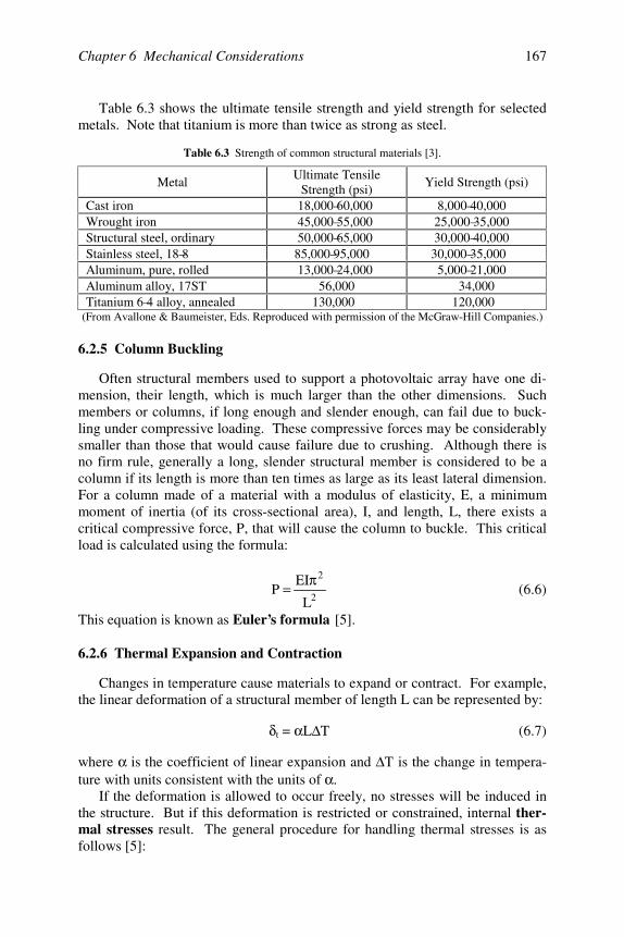
Chapter 6 Mechanical Considerations 167
Table 6.3 shows the ultimate tensile strength and yield strength for selectedmetals. Note that titanium is more than twice as strong as steel.
Table 6.3 Strength of common structural materials [3].
MetalUltimate Tensile
Strength (psi)Yield Strength (psi)
Cast iron 18,000–60,000 8,000–40,000Wrought iron 45,000–55,000 25,000–35,000Structural steel, ordinary 50,000–65,000 30,000–40,000Stainless steel, 18–8 85,000–95,000 30,000–35,000Aluminum, pure, rolled 13,000–24,000 5,000–21,000Aluminum alloy, 17ST 56,000 34,000Titanium 6–4 alloy, annealed 130,000 120,000
(From Avallone & Baumeister, Eds. Reproduced with permission of the McGraw-Hill Companies.)
6.2.5 Column Buckling
Often structural members used to support a photovoltaic array have one di-mension, their length, which is much larger than the other dimensions. Suchmembers or columns, if long enough and slender enough, can fail due to buck-ling under compressive loading. These compressive forces may be considerablysmaller than those that would cause failure due to crushing. Although there isno firm rule, generally a long, slender structural member is considered to be acolumn if its length is more than ten times as large as its least lateral dimension.For a column made of a material with a modulus of elasticity, E, a minimummoment of inertia (of its cross-sectional area), I, and length, L, there exists acritical compressive force, P, that will cause the column to buckle. This criticalload is calculated using the formula:
2
2
L
EIP
π= (6.6)
This equation is known as Euler’s formula [5].
6.2.6 Thermal Expansion and Contraction
Changes in temperature cause materials to expand or contract. For example,the linear deformation of a structural member of length L can be represented by:
δ t = α L∆ T (6.7)
where α is the coefficient of linear expansion and ∆ T is the change in tempera-ture with units consistent with the units of α .
If the deformation is allowed to occur freely, no stresses will be induced inthe structure. But if this deformation is restricted or constrained, internal ther-mal stresses result. The general procedure for handling thermal stresses is asfollows [5]:
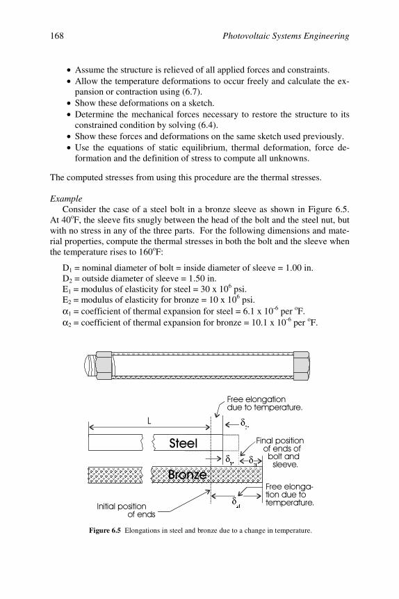
Photovoltaic Systems Engineering168
• Assume the structure is relieved of all applied forces and constraints.• Allow the temperature deformations to occur freely and calculate the ex-
pansion or contraction using (6.7).• Show these deformations on a sketch.• Determine the mechanical forces necessary to restore the structure to its
constrained condition by solving (6.4).• Show these forces and deformations on the same sketch used previously.• Use the equations of static equilibrium, thermal deformation, force de-
formation and the definition of stress to compute all unknowns.
The computed stresses from using this procedure are the thermal stresses.
ExampleConsider the case of a steel bolt in a bronze sleeve as shown in Figure 6.5.
At 40oF, the sleeve fits snugly between the head of the bolt and the steel nut, butwith no stress in any of the three parts. For the following dimensions and mate-rial properties, compute the thermal stresses in both the bolt and the sleeve whenthe temperature rises to 160oF:
D1 = nominal diameter of bolt = inside diameter of sleeve = 1.00 in.D2 = outside diameter of sleeve = 1.50 in.E1 = modulus of elasticity for steel = 30 x 106 psi.E2 = modulus of elasticity for bronze = 10 x 106 psi.α 1 = coefficient of thermal expansion for steel = 6.1 x 10⁻⁶ per oF.α 2 = coefficient of thermal expansion for bronze = 10.1 x 10⁻⁶ per oF.
!!" #
$ !
δI
δW
δW
δ2 I
Figure 6.5 Elongations in steel and bronze due to a change in temperature.
Chapter 6 Mechanical Considerations 169
To solve this problem, note first that the elongation of the bronze sleevewould be greater than that for the steel bolt if both were unconstrained. For anylength L, these elongations could be calculated using equation (6.7). However,the bolt head and nut constrain the sleeve so that the elongations of both thesleeve and bolt must be equal. Hence, the sleeve is in compression and the boltis in tension. Also, from the principle of action and reaction, the compressiveforce in the sleeve must be equal and opposite to the tensile force in the bolt.
From the sketch in Figure 6.5, the total elongations of the bolt and sleeve are,respectively:
1 1 1 1t 1f (steel bolt)2 2 2 2t 2f (bronze sleeve)
Equating the forces, elongations and applying equations (6.4) and (6.7) yields:
1)(L)(T2-T1) + PL/[(A1)(E1 2)(L)(T2-T1) – PL/[(A 2)(E2)]
The length, L, is a common term and cancels. Solving for the force, P, gives:
P = 3,330 lb.
The normal stresses in the bolt are computed using equation (6.1) and are:
S1 = 4,240 psi (tension) and S2 = 3,390 psi (compression)
6.2.7 Chemical Corrosion and Ultraviolet Degradation
A photovoltaic system structure that can initially withstand all anticipatedmechanical and thermal stresses with an adequate margin of safety might not bea good engineering design. The engineer must also consider the environment inwhich the system operates and how its component materials interact with theenvironment and with each other. Failure of metal components by corrosion isas common as failure due to mechanical stresses.
To design for corrosion resistance, knowledge of the various forms of corro-sion is necessary.
Uniform attack is the most common form of corrosion. Chemical or elec-trochemical reactions proceed uniformly over the entire surface area. The metalbecomes thinner and thinner and eventually fails. On a tonnage basis, uniformattack is the greatest cause of metal destruction, especially steel. However, it isnot particularly difficult to control through proper material selection and appro-priate use of protective coatings.
Galvanic corrosion occurs because of the potential difference that existsbetween two dissimilar metals in contact with a corrosive or conducting solu-tion. Of the two dissimilar metals, the less resistant, or anodic, metal is corrodedrelative to the more resistant, or cathodic, metal. Table 6.4 presents an abbrevi-
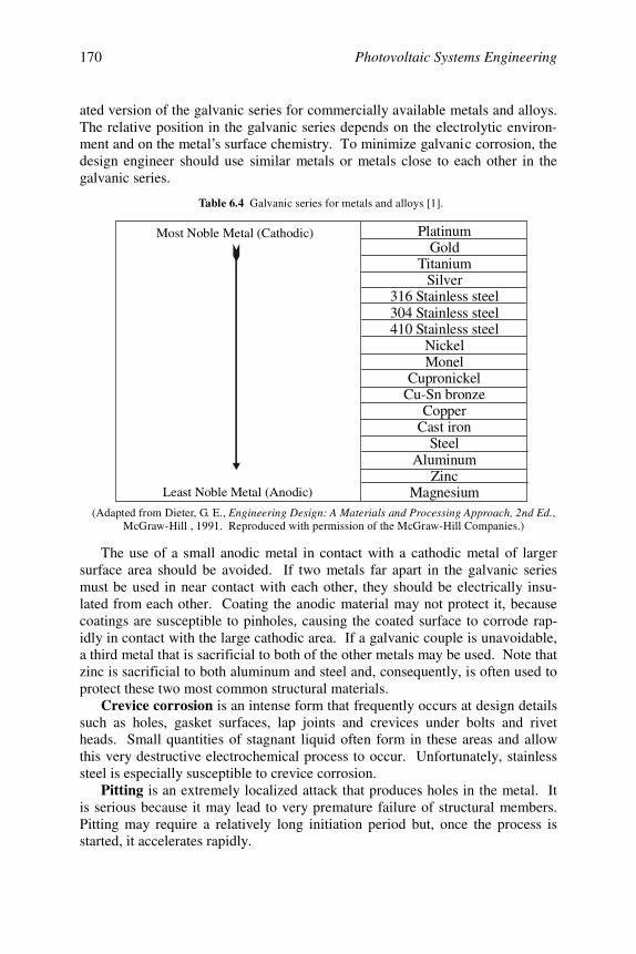
Photovoltaic Systems Engineering170
ated version of the galvanic series for commercially available metals and alloys.The relative position in the galvanic series depends on the electrolytic environ-ment and on the metal’s surface chemistry. To minimize galvanic corrosion, thedesign engineer should use similar metals or metals close to each other in thegalvanic series.
The use of a small anodic metal in contact with a cathodic metal of largersurface area should be avoided. If two metals far apart in the galvanic seriesmust be used in near contact with each other, they should be electrically insu-lated from each other. Coating the anodic material may not protect it, becausecoatings are susceptible to pinholes, causing the coated surface to corrode rap-idly in contact with the large cathodic area. If a galvanic couple is unavoidable,a third metal that is sacrificial to both of the other metals may be used. Note thatzinc is sacrificial to both aluminum and steel and, consequently, is often used toprotect these two most common structural materials.
Crevice corrosion is an intense form that frequently occurs at design detailssuch as holes, gasket surfaces, lap joints and crevices under bolts and rivetheads. Small quantities of stagnant liquid often form in these areas and allowthis very destructive electrochemical process to occur. Unfortunately, stainlesssteel is especially susceptible to crevice corrosion.
Pitting is an extremely localized attack that produces holes in the metal. Itis serious because it may lead to very premature failure of structural members.Pitting may require a relatively long initiation period but, once the process isstarted, it accelerates rapidly.
Most Noble Metal (Cathodic) PlatinumGold
TitaniumSilver
316 Stainless steel304 Stainless steel410 Stainless steel
NickelMonel
CupronickelCu-Sn bronze
CopperCast iron
SteelAluminum
ZincMagnesiumLeast Noble Metal (Anodic)
Table 6.4 Galvanic series for metals and alloys [1].
(Adapted from Dieter, G. E., ,McGraw-Hill , 1991. Reproduced with permission of the McGraw-Hill Companies.)
Engineering Design: A Materials and Processing Approach, 2nd Ed.

Chapter 6 Mechanical Considerations 171
Intergranular corrosion is a localized attack along the grain boundaries ofmetals but not (or only slightly) over the grain faces. It is common in steel thathas been heat treated at high temperatures or heat sensitized during welding.Intergranular corrosion due to welding is known as weld decay.
Selective leaching is the preferential removal of one or more of the alloyingelements in a metal by the action of an electrolyte. The most common exampleof this phenomenon is the selective leaching of zinc from brass, leaving aspongy, weak matrix of copper – a process known as dezincification. Alumi-num, iron, cobalt and chromium are also susceptible to leaching. Where andwhenever selective leaching occurs, the process leaves the alloy in a weakened,porous condition.
Erosion corrosion occurs when corrosive fluid flows over a metal surfaceand causes the gradual wearing away of the surface. Usually the velocity of thefluid is high and mechanical wear and abrasion may be involved.
Stress corrosion cracking is caused by the combination of tensile stress andcorrosion and leads to the cracking or embrittlement of a metal. The stress mayresult from applied forces or may be residual. Only specific combinations ofalloys and the chemical environment produce stress corrosion cracking. Combi-nations include aluminum alloys and saltwater, some steel alloys and saltwateras well as mild steel and caustic soda. Preventing stress corrosion cracking in-volves selecting alloys that are not susceptible to cracking under expected oper-ating conditions. If this is not possible, the structural members should be sizedfor low stress levels.
Dry corrosion involves reaction of the material directly with air. Virtuallyevery metal and alloy reacts with the oxygen in air to form an oxide. This oc-curs in the absence of any liquid electrolyte and is an important form of corro-sion in high temperature applications.
In addition to corrosion, ultraviolet radiation can cause degradation and dete-rioration of some of the exposed materials used in photovoltaic systems. Theseinclude weather-sealing materials, conduit for wiring, wire insulation, somecoatings and caulking and other miscellaneous materials.
Ultraviolet radiation is that part of the electromagnetic spectrum havingwavelengths between about 100 and 400 nm. The ultraviolet portion of thespectrum can be further subdivided into three regions: UV-A (315–400 nm),UV-B (280–315 nm) and UV-C (100–280 nm). UV-B and UV-C cause s unburn(erythema) and pigmentation (tanning). UV-B produces vitamin D3. Long-termexposure to UV radiation results in loss of skin elasticity. Also, a link has beenestablished between exposure to UV wavelengths below 320 nm and skin can-cer. Because the human body is seriously affected by UV exposure, it shouldcome as no surprise that other materials are also affected. In fact, ultravioletradiation degrades both the optical properties and the physical properties ofmany materials. Consequently, the design engineer should ensure that all mate-rials in the photovoltaic system that are exposed to sunlight are resistant to UVdegradation.

Photovoltaic Systems Engineering172
6.2.8 Properties of Steel
Iron is the base element of all steels. Commercially pure iron contains onlyabout 0.01% carbon and is relatively soft and weak. The addition of carbonsignificantly strengthens iron. For example, the addition of 0.80% carbon canraise the tensile strength from about 40,000 psi to 110,000 psi [6]. Steel is analloy of iron and carbon and usually contains small amounts of manganese andother elements. There are more than 3,500 grades of steel, of which 75 percenthave been developed over the last 20 years. The many different grades of steelhave many different properties: physical, chemical and environmental. Carbonsteel is steel that owes its distinctive properties to the carbon it contains. Alloysteel is steel that owes its distinctive properties to one or more elements otherthan carbon, or to the combination of these elements with carbon.
For any material, steel or otherwise, it is easy to measure its chemical com-position and to determine its stress-strain curve using a pull test. The latter pro-vides the yield strength, tensile strength, elongation and reduction in area.However, the photovoltaic engineer must not forget to consider costs, corrosionresistance and the possibility of structural fatigue as well.
Low-carbon steel is often used in the support structures for photovoltaicsystems. Of the many low-carbon steel products, sheet and strip steels are be-coming increasingly important and presently account for approximately 60% ofthe total steel production in the U.S. [3]. The relatively low cost of these steelproducts gives them a major advantage over more expensive aluminum, pro-vided they can be protected adequately from corrosion.
Many different methods are used to protect steel from corrosion. In general,these protection or reduction methods include proper selection of materials, de-sign, coatings, inhibitors, anodic protection and cathodic protection [3]. Onemethod of protecting steel structural members is hot-dip galvanizing. Hot-dipgalvanizing is a process in which thoroughly cleaned steel or iron is immersed inmolten zinc and withdrawn to provide a smooth, even coating that typically hasa crystalline appearance. It is by far the most widely used method for protectingsteel against corrosion [6].
Zinc is a less noble metal than steel (see Table 6.4) and is sacrificed to pro-tect the steel as part of the corrosion process. How long the zinc protects thesteel depends on the thickness of the zinc coating and the environment to whichthe structural member is exposed. The average minimum weight of zinc coatingis 1.5 ounces per square foot of surface area when hot-dip galvanized accordingto the specifications of ASTM A123. For highly acidic industrial atmospheres, a1.5 ounce per square foot coating may last less than 15 years. For a rural, cleanatmosphere, the same coating may last 40 years.
The largest use of zinc is for protectively coating steel. Lead is sometimesadded to the zinc to produce a surface pattern called spangle, which is oftenused on unpainted surfaces. The addition of aluminum to zinc improves its cor-rosion protection ability. Galfan, which contains 5 percent aluminum and 95percent zinc, and Galvalume, which contains 55 percent aluminum and 45 per-

Chapter 6 Mechanical Considerations 173
cent zinc, are examples of zinc-aluminum coatings that effectively protect steelfrom corrosion [3].
Paints, lacquers, coal-tar or asphalt enamels, waxes and varnishes are allused as organic coatings for corrosion protection. However, all paints are per-meable to water and oxygen to some degree. They are also subject to mechani-cal damage and eventually break down.
6.2.9 Properties of Aluminum
Aluminum is the second most commonly used structural material next tosteel. Some of the properties of aluminum that make it attractive for use inphotovoltaic systems follow:
• It is very lightweight, with a density about one-third that of steel.• It can be fabricated into many different shapes using a variety of dif-
ferent methods.• It has a wide range of properties and is available at many different
tensile strengths, depending on how it is alloyed.• It has a high strength-to-weight ratio, thus making it attractive for
many applications.• It has good corrosion resistance and can be used in a wide variety of
climates and weather conditions.• It is available in a wide variety of finishes making it attractive as an
architectural metal.
Aluminum is one of the most fascinating of all the elements. It is verychemically active, with a strong affinity for oxygen. In powdered form, it isused as a fuel for solid rocket motors. How can it be that such a chemically ac-tive material is so commonly used in an unprotected form?
What makes aluminum unique is its special relationship with oxygen, whichdestroys other reactive metals such as sodium and seriously attacks less reactivemetals such as iron. In the laboratory, most chemistry students have witnessedthe spectacular reaction between sodium and the oxygen in water, in which thesodium is left unrecognizable and even more unusable. And everybody fre-quently encounters rusting steel. Neither of these phenomena occurs with alu-minum. Rather, as soon as aluminum is produced, its surface reacts with theoxygen in the air and forms a very thin oxide layer over the entire surface. Thisoxide layer is hard, tenacious and not only protects the aluminum from attack byother chemicals, but also protects it from further oxidation. Because the oxidelayer is transparent, it does not detract from the metal’s appearance. Aluminumoxide must be removed from aluminum wire before connections are made.
Pure aluminum is relatively weak and only about one third as stiff as steel.However, aluminum can be strengthened significantly by alloying. The mostcommon alloying additions to aluminum are copper, manganese, silicon, magne-sium and zinc.
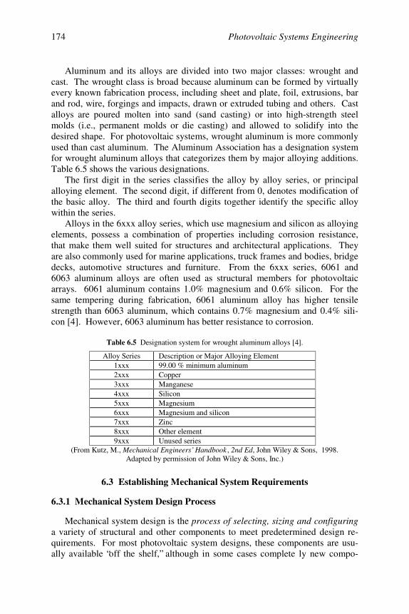
Photovoltaic Systems Engineering174
Aluminum and its alloys are divided into two major classes: wrought andcast. The wrought class is broad because aluminum can be formed by virtuallyevery known fabrication process, including sheet and plate, foil, extrusions, barand rod, wire, forgings and impacts, drawn or extruded tubing and others. Castalloys are poured molten into sand (sand casting) or into high-strength steelmolds (i.e., permanent molds or die casting) and allowed to solidify into thedesired shape. For photovoltaic systems, wrought aluminum is more commonlyused than cast aluminum. The Aluminum Association has a designation systemfor wrought aluminum alloys that categorizes them by major alloying additions.Table 6.5 shows the various designations.
The first digit in the series classifies the alloy by alloy series, or principalalloying element. The second digit, if different from 0, denotes modification ofthe basic alloy. The third and fourth digits together identify the specific alloywithin the series.
Alloys in the 6xxx alloy series, which use magnesium and silicon as alloyingelements, possess a combination of properties including corrosion resistance,that make them well suited for structures and architectural applications. Theyare also commonly used for marine applications, truck frames and bodies, bridgedecks, automotive structures and furniture. From the 6xxx series, 6061 and6063 aluminum alloys are often used as structural members for photovoltaicarrays. 6061 aluminum contains 1.0% magnesium and 0.6% silicon. For thesame tempering during fabrication, 6061 aluminum alloy has higher tensilestrength than 6063 aluminum, which contains 0.7% magnesium and 0.4% sili-con [4]. However, 6063 aluminum has better resistance to corrosion.
Table 6.5 Designation system for wrought aluminum alloys [4].
Alloy Series Description or Major Alloying Element1xxx 99.00 % minimum aluminum2xxx Copper3xxx Manganese4xxx Silicon5xxx Magnesium6xxx Magnesium and silicon7xxx Zinc8xxx Other element9xxx Unused series
(From Kutz, M., Mechanical Engineers’ Handbook , 2nd Ed, John Wiley & Sons, 1998.Adapted by permission of John Wiley & Sons, Inc.)
6.3 Establishing Mechanical System Requirements
6.3.1 Mechanical System Design Process
Mechanical system design is the process of selecting, sizing and configuringa variety of structural and other components to meet predetermined design re-quirements. For most photovoltaic system designs, these components are usu-ally available “off the shelf,” although in some cases complete ly new compo-

Chapter 6 Mechanical Considerations 175
nents may need to be developed. The challenge is to bring together componentsof the appropriate materials, geometric shapes and sizes to produce a system thatbest meets the design objectives.
The design requirements for the mechanical system consist of the following:
• Functional requirements• Operational requirements• Constraints• Tradeoffs.
Developing specifications for each of the above four categories is not uniqueto photovoltaic system design. It is commonly used in the design of systems ingeneral, including aircraft, satellites and other products of modern society [7].Determining the information to include in each of the four categories is an im-portant responsibility assumed by the systems engineer at an early stage in thedesign process.
6.3.2 Functional Requirements
What are the primary functions of the mechanical parts of the photovoltaicsystem? First and foremost, the mechanical system must be capable of carryingall expected mechanical forces with an adequate margin of safety. In fact, themost important requirement for both the mechanical and electrical design of thephotovoltaic system is the safety of individuals and the protection of structuresand other property that could be damaged as the result of mechanical failure.The functional requirement related to structural considerations might take sev-eral forms, such as the specification of factors of safety, or maximum allowablestresses, or limits on deformation. This specification will affect the materialsselected, as well as the geometry and size of the structural members.
For most designs, the photovoltaic array and support structure must with-stand all forces and associated stresses to which they are subjected for 20 to 30years or longer. Often they must do so in harsh weather and chemical environ-ments. These environments cause many materials to degrade, deteriorate andeventually fail. Consequently, the specification of the lifetimes of the structuralmembers and other materials that make up the photovoltaic system is an impor-tant functional requirement. This specification will affect not only the materialsselected, but also the selection of protective coatings that may be necessary toprotect these materials from corrosion and other forms of environmental degra-dation over the anticipated life of the system.
Some photovoltaic systems track the sun, using either single or double axistracking. The function of the tracking subsystem is to provide increased expo-sure to the sun’s radiation. Therefore, another type of functional requirement isthe specification of the required motion of the tracking system. This specifica-tion is especially important for concentrating arrays and affects the design of thedrive mechanism for the tracker.
Photovoltaic Systems Engineering176
6.3.3 Operational Requirements
Operational requirements involve the more important aspects of the designthat affect the people who install, own, operate, maintain, repair and/or servicethe photovoltaic system. An example of an operational requirement would be aspecification of the maximum labor hours required to assemble and install aphotovoltaic system. This type of specification is becoming increasingly im-portant as industry tries to reduce the costs of photovoltaic system installations.It has a major effect on the simplicity of the design and the ease of assembly ofthe system.
A specification related to accessibility, especially accessibility to individualmodules and other critical components for inspection, maintenance and repair, isanother type of operational requirement. It affects the size and shape of selectedmechanical components and how they are configured.
For some photovoltaic system designs, the specification of security require-ments may be necessary. This type of specification is used to protect againstvandalism, theft and personal injury and affects the selection and configurationof components. For example, the operational requirement to protect photovol-taic modules from flying objects has led to the frequent use of shielding on theback of small arrays for area lighting systems. Security requirements have alsoled the engineer to designs that include buried or tamper-proof enclosures.
Another type of operational requirement is the specification of periodic in-spection and maintenance. For example, the requirement for seasonally adjust-ing array tilt angles affects the selection and configuration of structural supportcomponents. Anticipated rain, snow, ice, dust and the presence of birds, predis-posed to target arrays with their droppings, are all examples of conditions thathave affected the operational specifications for photovoltaic system designs.
6.3.4 Constraints
Invariably, the process of engineering design is constrained or limited insome way. The most common design constraint is cost. In the highly competi-tive renewable energy marketplace, it is important to keep costs to a minimum.Cost constraints have a major effect on system design. For example, aluminummay be the preferred structural material for the mechanical system because of itsresistance to corrosion. But steel may be the material of choice because it isconsiderably less expensive, even after it has been hot-dip galvanized. Costconstraints are omnipresent and pervasive, and they challenge the ingenuity ofthe design engineer. Typically, the photovoltaic system must be designed andinstalled within a specified budget.
Another design constraint is time. Good design, in all of its creative aspects,takes precious time—and sufficient time is not always available to satisfy theinner needs of the design engineer. Typically, the photovoltaic system must bedesigned and installed according to a specified schedule.
From time to time, the design engineer will be confronted with other types ofconstraints. Limited access to the sun due to existing or imminent shading (e.g.,

Chapter 6 Mechanical Considerations 177
due to proposed construction) is commonplace. Restrictive building codes,covenants and zoning may prohibit the installation of a photovoltaic system orlimit the design options. The same can be said for political, regulatory and in-stitutional issues. And finally, the effects of weather, location and site layoutoften need to be considered before getting too far into the design process.
In summary, constraints are a reflection of the real world in which the engi-neer operates. They usually have a major effect on design decisions and, conse-quently, should be included in the specification of design requirements. A clearunderstanding of these constraints will assist the engineer in producing a bettermechanical design.
6.3.5 Tradeoffs
Specifying the functional and operational requirements establishes the de-sired objectives for the mechanical system design. In a sense, it is a sophisti-cated wish list: the structure should be strong; the materials should last a longtime; they should resist corrosion and other forms of degradation; and the arrayshould have a certain orientation or possibly track the sun. In addition, the sys-tem should be easy to assemble in a short period of time; important componentsshould be readily accessible to work on; it should be protected from vandals andthieves; and it should be easy to maintain. On the other hand, a listing of theconstraints emerges: the costs are too high; the schedule cannot be met; the arraymust be moved to avoid shading; restrictive covenants may be violated; the gridinterconnection requirements are unreasonable; and the weather is marginal forsolar. In short, because of the constraints, the desired objectives cannot be metand it is time to compromise.
When the desired objectives cannot be met, the following items are subjectto compromise: quality or performance, cost and schedule. There is an old say-ing: “Pick any two and trade down on the third.” Assuming the cost and sched-ule constraints are rigid (they may not be), the engineer has to decide whichtradeoffs in quality and performance are acceptable. Examples of tradeoffs toreduce costs and operate within budget include using steel rather than aluminum,using lower factors of safety, using lower grade steel, using less expensive cor-rosion inhibitors, eliminating tracking, using less expensive and probably lessskilled installers and using less expensive security measures. Examples oftradeoffs to meet schedule include substituting readily available structural mem-bers for preferred parts, eliminating certain design features and using readilyavailable labor.
6.4 Design and Installation Guidelines
6.4.1 Standards and Codes
Prior to the establishment of modern standards, structural members, nuts,bolts, screws and so on, were custom designed and manufactured. For example,one manufacturer would produce ½-inch bolts with 9 threads per inch, while

Photovoltaic Systems Engineering178
another would use 12 threads per inch. Some fasteners had left-handed threadsand had different thread profiles. In the early days of the automobile, mechanicswould lay out fasteners in a row as they were disassembled to avoid mixingthem during reassembly. A lack of standards leads to a lack of uniformity andprecludes efficient interchangeability of parts. It is inefficient and costly.
A standard is a set of specifications for parts, materials or processes in-tended to achieve uniformity, efficiency and a specified quality. Another im-portant purpose of standards is to limit the number of items in the specificationand thereby provide a reasonable inventory of tooling, sizes and varieties socustom parts will not be required.
A code is a set of specifications for the analysis, design, manufacture, con-struction or installation of something. The purpose of a code is to achieve aspecified degree of safety, efficiency and performance or quality. It should benoted that safety codes do not imply absolute safety, which is impossible to at-tain. Designing a structure to withstand 120-mph winds does not mean the de-signer thinks 140-mph winds are impossible. It just means the designer thinksthey are highly improbable.
The following organizations are involved in developing standards and codesrelevant to the mechanical design of photovoltaic systems:
• Aluminum Association (AA)• American Institute of Steel Construction (AISC)• American Iron and Steel Institute (AISI)• American Society of Civil Engineers (ASCE)• American Society of Metals (ASM)• American Society of Mechanical Engineers (ASME)• American Society of Testing and Materials (ASTM)• Society of Automotive Engineers (SAE).
Building codes are design, construction and installation guidelines. They areadopted and enforced by local jurisdictions to help ensure the safety of individu-als and the protection of structures and other property in and around buildings.Building and electrical codes have value only if they are followed and enforced.The process begins prior to the installation of a photovoltaic system with an ap-plication for a building permit. After the installation, the building official in-spects the system to determine compliance with the relevant codes. Unfortu-nately, many solar systems have been installed in the past without first obtaininga building permit. Most photovoltaic systems installed prior to the mid-1990swere stand-alone systems and probably would not meet present code require-ments. However, with the renewed interest in photovoltaic systems for build-ings as a result of financial incentive programs and government initiatives, mostnew systems comply with local codes. And utility-interactive photovoltaic sys-tems are more likely to be inspected by building code officials than are stand-alone systems.

Chapter 6 Mechanical Considerations 179
6.4.2 Building Code Requirements
The most important standard affecting the mechanical design of photovoltaicsystems is entitled Minimum Design Loads for Buildings and Other Structures[8]. It is a standard of the American Society of Civil Engineers and is periodi-cally updated. It provides the minimum load carrying requirements for build-ings and other structures, and these requirements apply to photovoltaic systems.It is important to note that standards have meaning only when they are adoptedby an enforcing jurisdiction and become part of their code. Many local jurisdic-tions reference parts of this ASCE standard in their building codes. However,local building codes are less uniform than local electrical codes, almost all ofwhich use the National Electrical Code (NEC).
The basic requirements of building codes are that the photovoltaic systemand any building or other structure to which it is attached, shall be designed andconstructed to safely support any mechanical load or combination of loads towhich they are subjected. In other words, the ASCE standard provides formulasfor computing the mechanical loads from wind, snow, ice and so on. The engi-neer computes these loads for the conditions expected at the site of the photo-voltaic system. The stresses these forces produce must not exceed the appropri-ately specified allowable stresses for the structural materials being used.
In addition to establishing strength requirements, building codes often limitthe deformations that can occur with physical structures such as photovoltaicsystems. For example, there may be restrictions on the amount of deflection orlateral drift of a structure. Such a deflection might have an adverse effect on theuse of the system or attached buildings or structures. Because vibration can leadto fatigue failure, the local building code may contain provisions that address thestiffness of the structure and the associated frequencies and amplitudes ofstructural vibration.
6.5 Forces Acting on Photovoltaic Arrays
6.5.1 Structural Loading Considerations
Because solar energy is a relatively dilute resource, photovoltaic modulesand arrays are area intensive. These large-area solar electric devices are capableof transmitting a variety of forces to themselves, their support structures, build-ings and other frames or foundations to which they are mechanically attached.These forces include the dead weight of the array, the weight of array installa-tion and maintenance people and their equipment, aerodynamic wind loading,seismic effects and the forces due to rain, snow and ice. Determining theseforces under prescribed conditions can be an interesting and challenging me-chanics problem.
Of the various types of forces mentioned above, aerodynamic wind loadingpresents the most concern. At most locations around the world, the force effectsdue to wind loading are much higher than the other forces acting on the struc-

Photovoltaic Systems Engineering180
ture. For example, both dead and live weight loads due to a photovoltaic arrayon a building are usually less than five pounds per square foot (psf). In contrast,the computed wind loads are typically between 24 psf and 55 psf, depending onlocation and the associated design wind speed for that location.
Because of the geographic variation in environmental conditions such asrain, snow, ice, wind speed, seismic activity, etc., local building codes tend to bemuch less uniform than electrical codes. Consequently, it is important for thephotovoltaic systems engineer not only to become familiar with local buildingcode requirements, but also to compute the minimum structural design loads thatare relevant for a given location.
In addition to the above considerations, the design engineer must select andconfigure the array mounting materials so that corrosion and ultraviolet degra-dation are minimized. Also, if the array is mounted on a building, the structuralintegrity of the building must not be degraded and building penetrations must beproperly sealed so that the building remains watertight over the life of thephotovoltaic array.
The ASCE standard [8] provides instructions and formulas for computing thefollowing types of loads:
• Dead loads• Live loads• Soil and hydrostatic pressure and flood loads• Wind loads• Snow loads• Rain loads• Earthquake loads• Ice loads – atmospheric icing• Combinations of the above loads.
6.5.2 Dead Loads
Dead loads consist of the weight of all the materials that are supported by thestructural members, including the weights of the structural members themselves.As an example, consider a photovoltaic array mounted on the roof of a building.The modules are structurally tied together in panels using steel or aluminumstructural members. The weight of the modules is carried by the structuralmembers and transmitted to the roof structure of the building. The total deadload that the roof must carry is the combined weight of the modules, structuralmembers used to form the panels, attachment hardware and mounting brackets.These loads can be expressed in pounds per square foot (psf) and assumed to actuniformly over the area covered by the array. Or the equations of static equilib-rium can be used to determine the individual forces at each of the brackets thatconnect the panels to the roof. For photovoltaic systems, the dead loads are usu-ally assumed to act uniformly over the supporting structure and are expressed in
Chapter 6 Mechanical Considerations 181
pounds per square foot. Note that these are external loads—not internalstresses—even though similar units are used.
Dead loads for photovoltaic systems generally fall within the range of 2 to 5psf and, even though they cannot be discounted, do not pose serious structuralproblems for the engineer.
6.5.3 Live Loads
Live loads associated with photovoltaic systems are those produced by indi-viduals and their equipment and materials during installation, inspection andmaintenance. In designing structures to carry live loads, the engineer may treatthem as uniformly distributed loads, i.e., in psf, as concentrated loads (lb) or as acombination of uniformly distributed and concentrated loads. For photovoltaicarrays, live loads are usually assumed to be distributed uniformly and are small,on the order of 3 psf or less.
6.5.4 Wind Loads
The forces from the wind acting on photovoltaic arrays are aerodynamicforces. As such, their magnitudes depend partly on the properties of the atmos-phere. Atmospheric properties include static pressure, temperature, viscosityand density. Of these, density is one of the more important ones affecting themechanical forces acting on photovoltaic systems. At any given location, den-sity is usually assumed to be constant. However, density does vary with alti-tude decreasing as altitude is increased. For example, the density in the mile-high city of Denver, CO, is about 86% of the atmospheric density for Floridacities, which are only slightly above sea level. The mass density of air for thestandard atmosphere at sea level is 0.00256 lb-sec2/ft4.
The air flowing over a photovoltaic array produces two types of forces:pressure forces normal to the surface and skin friction forces along the sur-face. Skin friction forces are simply surface shear forces resulting from the vis-cosity of the air as it contacts the surface.
Obtaining a better idea of the important relationships affecting the flow of airover structures requires some simplifying assumptions. First, assume the flowof air is inviscid, which implies that the viscosity of the air is zero. Next, as-sume that the flow of air is incompressible, which implies that the density ofthe air is constant. Finally, assume the flow of air is conservative, which im-plies that there are no other energy dissipating processes. With these assump-tions, the linear momentum equation for fluid flow reduces to [9]:
(6.8)
where V = wind speed, g = acceleration due to gravity, z = altitude or elevation,p = static pressure and ρ = mass density. Integrating each term yields:
( )∫ ∫ ∫ =ρ
++ constantdp
gdzVd21 2
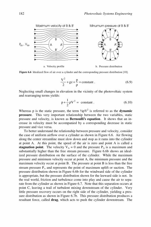
Photovoltaic Systems Engineering182
=ρ
++ pgz
2
V 2
constant . (6.9)
Neglecting small changes in elevation in the vicinity of the photovoltaic systemand rearranging terms yields:
=ρ+ 2V21
p constant . (6.10)
Whereas p is the static pressure, the term ½ρ V2 is referred to as the dynamicpressure. This very important relationship between the two variables, staticpressure and velocity, is known as Bernoulli’s equation . It shows that an in-crease in velocity must be accompanied by a corresponding decrease in staticpressure and vice versa.
To better understand the relationship between pressure and velocity, considerthe case of uniform airflow over a cylinder as shown in Figure 6.6. Air flowingalong the center streamline must slow down and stop as it rams into the cylinderat point A. At this point, the speed of the air is zero and point A is called astagnation point. The velocity VA = 0 and the pressure PA is a maximum andsubstantially higher than the free stream pressure. Figure 6.6b shows an ideal-ized pressure distribution on the surface of the cylinder. While the maximumpressure and minimum velocity occur at point A, the minimum pressure and themaximum velocity occur at point B. The pressure at point B is less than the freestream pressure P ∞ and represents the point of maximum uplift or suction. Thepressure distribution shown in Figure 6.6b for the windward side of the cylinderis appropriate, but the pressure distribution shown for the leeward side is not. Inthe real world, friction and turbulence come into play and cause the air to sepa-rate from the cylinder as shown in Figure 6.7. Note that this separation occurs atpoint C, leaving a trail of turbulent mixing downstream of the cylinder. Verylittle pressure recovery occurs on the right side of the cylinder, yielding a pres-sure distribution as shown in Figure 6.7b. This pressure distribution produces aresultant force, called drag, which acts to push the cylinder downstream. The
%
&
&'
' '
&
&'
( )#* &+&' ( &+&'
,
,
Figure 6.6 Idealized flow of air over a cylinder and the corresponding pressure distribution [10].
a. Velocity profile b. Pressure distribution
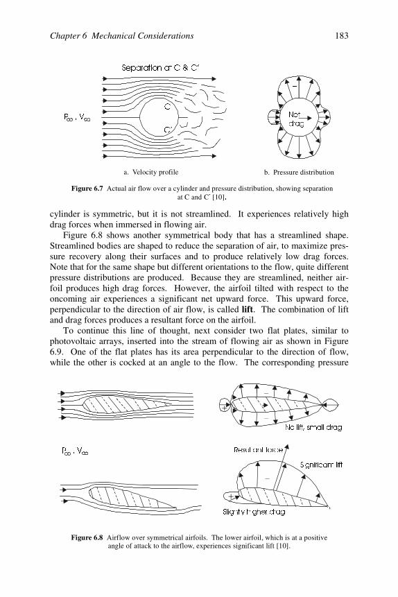
Chapter 6 Mechanical Considerations 183
cylinder is symmetric, but it is not streamlined. It experiences relatively highdrag forces when immersed in flowing air.
Figure 6.8 shows another symmetrical body that has a streamlined shape.Streamlined bodies are shaped to reduce the separation of air, to maximize pres-sure recovery along their surfaces and to produce relatively low drag forces.Note that for the same shape but different orientations to the flow, quite differentpressure distributions are produced. Because they are streamlined, neither air-foil produces high drag forces. However, the airfoil tilted with respect to theoncoming air experiences a significant net upward force. This upward force,perpendicular to the direction of air flow, is called lift. The combination of liftand drag forces produces a resultant force on the airfoil.
To continue this line of thought, next consider two flat plates, similar tophotovoltaic arrays, inserted into the stream of flowing air as shown in Figure6.9. One of the flat plates has its area perpendicular to the direction of flow,while the other is cocked at an angle to the flow. The corresponding pressure
3 9
B
6HSDUDWLRQDW&&·
&
&·
1HW
GUDJ
a. Velocity profile b. Pressure distribution
Figure 6.7 Actual air flow over a cylinder and pressure distribution, showing separationat C and C [10]·
3 9
1ROLIWVPDOOGUDJ
-
,
,
,
-
5HVXOWDQWIRUFH
6LJQLILFDQWOLIW
6OLJKWO\KLJKHUGUDJ
Figure 6.8 Airflow over symmetrical airfoils. The lower airfoil, which is at a positiveangle of attack to the airflow, experiences significant lift [10].
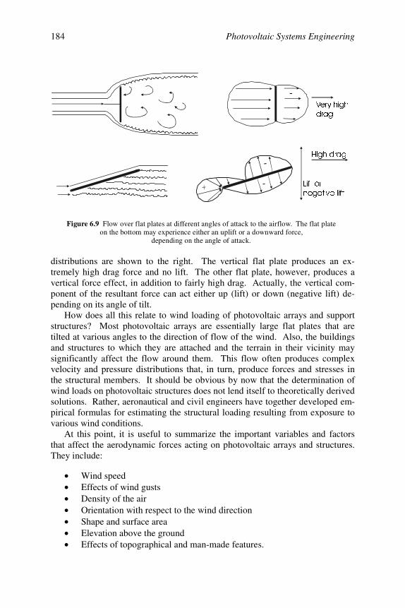
Photovoltaic Systems Engineering184
distributions are shown to the right. The vertical flat plate produces an ex-tremely high drag force and no lift. The other flat plate, however, produces avertical force effect, in addition to fairly high drag. Actually, the vertical com-ponent of the resultant force can act either up (lift) or down (negative lift) de-pending on its angle of tilt.
How does all this relate to wind loading of photovoltaic arrays and supportstructures? Most photovoltaic arrays are essentially large flat plates that aretilted at various angles to the direction of flow of the wind. Also, the buildingsand structures to which they are attached and the terrain in their vicinity maysignificantly affect the flow around them. This flow often produces complexvelocity and pressure distributions that, in turn, produce forces and stresses inthe structural members. It should be obvious by now that the determination ofwind loads on photovoltaic structures does not lend itself to theoretically derivedsolutions. Rather, aeronautical and civil engineers have together developed em-pirical formulas for estimating the structural loading resulting from exposure tovarious wind conditions.
At this point, it is useful to summarize the important variables and factorsthat affect the aerodynamic forces acting on photovoltaic arrays and structures.They include:
• Wind speed• Effects of wind gusts• Density of the air• Orientation with respect to the wind direction• Shape and surface area• Elevation above the ground• Effects of topographical and man-made features.
9HU\KLJK
GUDJ
+LJKGUDJ
/LIWRU
QHJDWLYHOLIW
Figure 6.9 Flow over flat plates at different angles of attack to the airflow. The flat plateon the bottom may experience either an uplift or a downward force,
depending on the angle of attack.
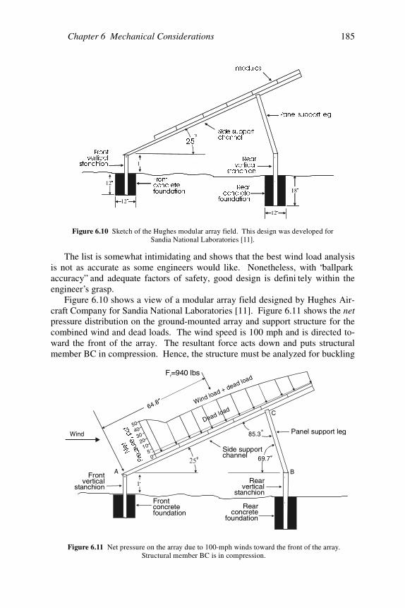
Chapter 6 Mechanical Considerations 185
The list is somewhat intimidating and shows that the best wind load analysisis not as accurate as some engineers would like. Nonetheless, with “ballparkaccuracy” and adequate factors of safety, good design is defini tely within theengineer’s grasp.
Figure 6.10 shows a view of a modular array field designed by Hughes Air-craft Company for Sandia National Laboratories [11]. Figure 6.11 shows the netpressure distribution on the ground-mounted array and support structure for thecombined wind and dead loads. The wind speed is 100 mph and is directed to-ward the front of the array. The resultant force acts down and puts structuralmember BC in compression. Hence, the structure must be analyzed for buckling
1·
Frontconcretefoundation
Rearconcrete
foundation
Frontvertical
stanchionRear
verticalstanchion
Side supportchannel
Panel support leg
F =940 lbsr
Wind load + dead load
Dead load
69.7
C
BA
05
1020
3040
50
64.8µ
Wind 85.3
1HW
3UHVVXUHSVI
Figure 6.11 Net pressure on the array due to 100-mph winds toward the front of the array.Structural member BC is in compression.
12µ
12µ
18µ
1·
PRGXOHV
12µ12µ
12µ12µ
18µ
1·
)URQWFRQFUHWHIRXQGDWLRQ
5HDUFRQFUHWH
IRXQGDWLRQ
)URQWYHUWLFDO
VWDQFKLRQ5HDU
YHUWLFDOVWDQFKLRQ
6LGHVXSSRUWFKDQQHO
3DQHOVXSSRUWOHJ
R
Figure 6.10 Sketch of the Hughes modular array field. This design was developed forSandia National Laboratories [11].
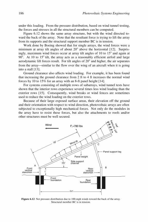
Photovoltaic Systems Engineering186
under this loading. From the pressure distribution, based on wind tunnel testing,the forces and stresses in all the structural members can be computed.
Figure 6.12 shows the same array structure, but with the wind directed to-ward the back of the array. Note that the resultant force is trying to lift the arrayfrom its supports and the structural support member BC is in tension.
Work done by Boeing showed that for single arrays, the wind forces were aminimum at array tilt angles of about 20o above the horizontal [12]. Surpris-ingly, maximum wind forces occur at array tilt angles of 10 to 15o and again at90o. At 10 to 15o tilt, the array acts as a reasonably efficient airfoil and largeaerodynamic lift forces result. For tilt angles of 20o and higher, the air separatesfrom the array similar to the flow over the wing of an aircraft when it is goinginto a stall [13].
Ground clearance also affects wind loading. For example, it has been foundthat increasing the ground clearance from 2 ft to 4 ft increases the normal windforces by 10 to 15% for an array with an 8-ft panel height [14].
For systems consisting of multiple rows of subarrays, wind tunnel tests haveshown that the interior rows experience several times less wind loading than theexterior rows [15]. Consequently, wind breaks or wind fences are sometimesused to reduce the wind loading on the exterior rows.
Because of their large exposed surface areas, their elevation off the groundand their orientation with respect to wind direction, photovoltaic arrays are oftensubjected to exceptionally high mechanical forces. Not only do the modules inthe array have to resist these forces, but also the attachments to roofs and/orother structures must be well secured.
1·
Frontfoundation Rear
foundation
Frontvertical
stanchion
Rearvertical
stanchion
Side supportchannel
Panel support leg
Panel weight
AB
C
Wind
76”Wind lift
F =780 lbsr
R
1HW
3UHVVXUHSVI
Figure 6.12 Net pressure distribution due to 100-mph winds toward the back of the array.Structural member BC is in tension.
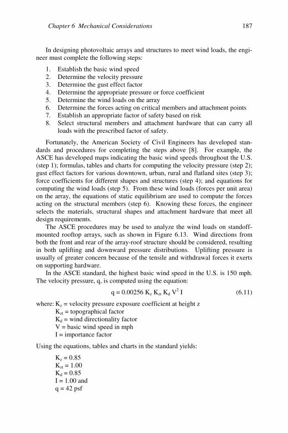
Chapter 6 Mechanical Considerations 187
In designing photovoltaic arrays and structures to meet wind loads, the engi-neer must complete the following steps:
1. Establish the basic wind speed2. Determine the velocity pressure3. Determine the gust effect factor4. Determine the appropriate pressure or force coefficient5. Determine the wind loads on the array6. Determine the forces acting on critical members and attachment points7. Establish an appropriate factor of safety based on risk8. Select structural members and attachment hardware that can carry all
loads with the prescribed factor of safety.
Fortunately, the American Society of Civil Engineers has developed stan-dards and procedures for completing the steps above [8]. For example, theASCE has developed maps indicating the basic wind speeds throughout the U.S.(step 1); formulas, tables and charts for computing the velocity pressure (step 2);gust effect factors for various downtown, urban, rural and flatland sites (step 3);force coefficients for different shapes and structures (step 4); and equations forcomputing the wind loads (step 5). From these wind loads (forces per unit area)on the array, the equations of static equilibrium are used to compute the forcesacting on the structural members (step 6). Knowing these forces, the engineerselects the materials, structural shapes and attachment hardware that meet alldesign requirements.
The ASCE procedures may be used to analyze the wind loads on standoff-mounted rooftop arrays, such as shown in Figure 6.13. Wind directions fromboth the front and rear of the array-roof structure should be considered, resultingin both uplifting and downward pressure distributions. Uplifting pressure isusually of greater concern because of the tensile and withdrawal forces it exertson supporting hardware.
In the ASCE standard, the highest basic wind speed in the U.S. is 150 mph.The velocity pressure, q, is computed using the equation:
q = 0.00256 Kz Kzt Kd V2 I (6.11)
where: Kz = velocity pressure exposure coefficient at height zKzt = topographical factorKd = wind directionality factorV = basic wind speed in mphI = importance factor
Using the equations, tables and charts in the standard yields:
Kz = 0.85Kzt = 1.00Kd = 0.85I = 1.00 andq = 42 psf
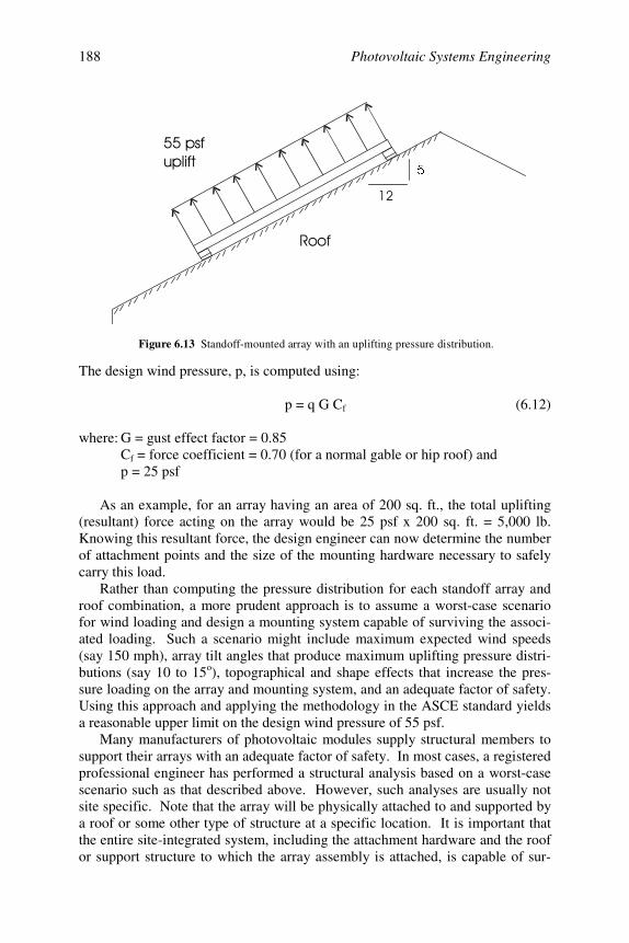
Photovoltaic Systems Engineering188
The design wind pressure, p, is computed using:
p = q G Cf (6.12)
where: G = gust effect factor = 0.85Cf = force coefficient = 0.70 (for a normal gable or hip roof) andp = 25 psf
As an example, for an array having an area of 200 sq. ft., the total uplifting(resultant) force acting on the array would be 25 psf x 200 sq. ft. = 5,000 lb.Knowing this resultant force, the design engineer can now determine the numberof attachment points and the size of the mounting hardware necessary to safelycarry this load.
Rather than computing the pressure distribution for each standoff array androof combination, a more prudent approach is to assume a worst-case scenariofor wind loading and design a mounting system capable of surviving the associ-ated loading. Such a scenario might include maximum expected wind speeds(say 150 mph), array tilt angles that produce maximum uplifting pressure distri-butions (say 10 to 15o), topographical and shape effects that increase the pres-sure loading on the array and mounting system, and an adequate factor of safety.Using this approach and applying the methodology in the ASCE standard yieldsa reasonable upper limit on the design wind pressure of 55 psf.
Many manufacturers of photovoltaic modules supply structural members tosupport their arrays with an adequate factor of safety. In most cases, a registeredprofessional engineer has performed a structural analysis based on a worst-casescenario such as that described above. However, such analyses are usually notsite specific. Note that the array will be physically attached to and supported bya roof or some other type of structure at a specific location. It is important thatthe entire site-integrated system, including the attachment hardware and the roofor support structure to which the array assembly is attached, is capable of sur-
Figure 6.13 Standoff-mounted array with an uplifting pressure distribution.

Chapter 6 Mechanical Considerations 189
viving the worst-case scenario of wind loading—not just the arr ay and mountingmembers that come with photovoltaic system package.
In summary, the largest mechanical forces acting on photovoltaic arrays andstructures are due to high wind speeds. Suppliers of packaged photovoltaicsystems should assume a worst-case wind loading of 55 psf (or higher) in de-signing their array mounting systems. Many have already done so. In addition,the entire integrated photovoltaic and building system must be able to survivethe worst-case scenario of wind loading and comply with all site-specific build-ing code requirements.
6.1.1 Snow Loads
Snow loads on photovoltaic arrays and on sloped roofs decrease as the tiltangles and slopes increase. There are three reasons for this. First, as the tiltangle increases, the component of the weight force parallel to the array surfaceincreases relative to the component normal to the array surface, thus helping toshed the snow. Second, wind forces tend to shed the snow from the array.Third, melt water reduces the friction between the array surface and helps toshed the snow. Most photovoltaic arrays have “slippery” glass surfaces that alsoaid the snow-shedding process. On the other hand, obstructions and rough sur-faces hinder the shedding of snow and its weight. For example, some tile roofscontain built-in protrusions or rough surfaces that prevent the snow from sliding.The snow that accumulates on arrays mounted on such roofs may be obstructedfrom shedding [8].
An extreme case of snow loading occurs when unusually large amounts ofsnow accumulate on an array at a relatively small tilt angle. However, this israre because shallow tilt angles are uncommon in colder, snow-prone parts ofthe world. In most cases, snow loads on photovoltaic arrays are less than 8 psf.
6.1.2 Other Loads
The photovoltaic array and support structure may experience mechanicalforces due to other loads, such as rain, ice, hydrostatic pressure and seismic ac-tivity. The latter is critical in earthquake-prone regions and the ASCE has de-tailed procedures for designing for seismic loads.
Foundations, footings or slabs that support photovoltaic arrays may experi-ence uplift forces due to hydrostatic pressure in locations where ground water isclose to the surface. If expansive soils are present, the hydrostatic pressures canbe quite large. In such cases, the expansive soils are sometimes excavated to adepth of at least 2 ft below ground level, followed by back filling with freelydraining sands and gravel.
Regardless of the location, the photovoltaic engineer is responsible for en-suring that all of the relevant loads and load combinations have been properlyaccounted for in the mechanical system design.

Photovoltaic Systems Engineering190
6.2 Array Mounting System Design
6.2.1 Introduction
Previous sections of this chapter discussed various properties of materials,the strength of materials, functional and operational requirements, standards andcodes and the mechanical forces acting on the array and support structure. Em-phasis was placed on material selection and compatibility based on concerns forstructural integrity, safety and code compliance. This section focuses on thoseaspects of the array mounting system that affect costs, performance, mainte-nance and appearance.
6.2.2 Objectives in Designing the Array Mounting System
In addition to meeting structural, code and safety requirements, good designof the array mounting system should achieve the following:
• Minimizing installation costs• Enhancing array performance• Providing reasonable accessibility for installation and maintenance• Making the system aesthetically appropriate for the site and application.
Minimizing Installation CostsBoth good design and good installation practices can be employed to reduce
installation costs. Studies in the 1990s by Sandia National Laboratories haveshown that only about half the cost of photovoltaic systems is for modules. Theother half is for nonmodule components and labor, with labor being the majorcontributor. For example, suppose a journeyman electrician installs a photovol-taic system. The electrical contractor may charge $75 per hour for the electri-cian’s time. The value of reducing the number of hours for installation shouldbe obvious. Photovoltaic manufacturers and system suppliers can reduce instal-lation costs by doing one or more of the following:
1. Developing packaged kits. For about the first 2 decades of applying photo-voltaics to terrestrial applications, system design was essentially customized foreach installation. Since the mid to late 1990s, the trend has been to developpackaged kits that can easily be adapted to a wide variety of installations.Building applications of photovoltaics have helped to accelerate this trend.Photovoltaic system suppliers now deliver standard models, which include mod-ules, the structural support systems, attachment hardware, batteries and invert-ers. Some include the module interconnect wiring, junction boxes and otherbalance-of-system components. The development and refinement of packagedkits should help reduce the cost of photovoltaic system installations.2. Minimizing the total number of parts. A second design approach to reduc-ing installation costs is to minimize the total number of parts included in thedesign. As an example, some suppliers are moving toward the use of larger

Chapter 6 Mechanical Considerations 191
modules and fewer panels. The idea is to use less-skilled personnel to assembleand prewire panels prior to shipment to the site. This reduces the time requiredby more highly skilled personnel to complete the installation at the site.3. Minimizing part variations. A third design approach to reducing installa-tion costs is to minimize part variations. This concept is easily applied to thesize and type of structural members, fasteners and attachment hardware. It ofteneliminates the need for special tooling.4. Designing parts to be multifunctional. Designing systems such that someparts are multifunctional is a fourth approach to cost reduction. For example, astructural member may be used not only to carry the mechanical loads, but alsoto enhance the flow of air over the back surface of the array.5. Designing parts for multiple uses. Structural members, brackets, attach-ment hardware and fasteners should be designed for possible use with differentkits, model numbers and product lines.6. Designing for ease of assembly. This not only reduces the time required toinstall systems, but also often results in higher reliability and reduced mainte-nance.7. Avoiding separate fasteners. One popular approach to reducing installationcosts is to use slotted roof brackets that allow photovoltaic modules or panels tobe simply dropped into the slots. It eliminates the need for on-site attachment ofnuts and bolts to connect the panels to roof brackets. Another alternative ap-proach is to use captive fasteners.8. Minimizing assembly direction. This means that parts should be designedso that they fit or can be assembled only one way the correct way. This iscommon practice in many industries.9. Maximizing compliance in assembly. The installer should not have tostruggle to assemble the panel framework, attach the modules to the panel, orattach the panels to the support structure. To maximize compliance in assembly,the designer should avoid tolerances that are too tight. Parts should fit togetherwith a minimum of effort.10. Minimizing handling in assembly and installation. This concept followsfrom a number of the other items, but also includes locating holes, slots andother points of attachment to reduce handling.
In addition to the design practices suggested above [1], good installationpractices can also be employed to reduce costs. Already mentioned is the prac-tice of preassembling and prewiring panels off-site using less-expensive person-nel. Another consideration for roof-mounted arrays is the number, type andplacement of roof attachment points. Often this decision is made by the installerat the site, rather than by the designer, and serious tradeoffs must be considered.For example, minimizing the number of roof attachments saves time, but it alsomeans that individual attachment points will be subjected to larger forces.
Building Integration ConsiderationsAs the population grows and building density increases, space becomes
more valuable and rooftops become more attractive locations for photovoltaic
Photovoltaic Systems Engineering192
arrays. The question arises: How can we most effectively integrate photovoltaicsystems and buildings? For existing buildings, the most prudent approach is touse designs that minimize costs by incorporating the measures discussed above.
Building-integrated photovoltaic (BIPV) products are solar electric devicesthat replace conventional building materials. They include solar shingles, tiles,skylights, windows, overhangs, facades, and PV laminates bonded directly tometal roofing panels. They can be used on either new or existing buildings in amanner that is aesthetically pleasing and very appealing to buyers.
For broad acceptance by builders and homeowners, more BIPV productsthat are attractive and easily incorporated into building construction are needed.As these new building-integrated photovoltaic products achieve attractive com-binations of costs and durability, they should further stimulate a growing marketfor rooftop applications.
However, widespread building-integrated photovoltaic applications may re-quire more than just new BIPV products. They may also require buildings withnew features that make them more receptive to photovoltaic systems. Examplesinclude innovative roof, truss and electrical system design. In addition, the inte-gration of on-site generation and super energy efficient buildings offers theprospect of alleviating national energy problems—from both the supply anddemand sides of the problem. The U.S. Department of Energy’s Zero EnergyHomes Program is a manifestation of the level of interest in this approach.
For new manufactured buildings, one interesting approach to building inte-gration involves factory-installed photovoltaic systems. Approximately 30% ofnew housing stock in the U.S. is manufactured housing. To be effective, themanufacture of buildings in a factory requires careful planning, time-motionstudies and process optimization—areas of interest to industria l engineers. Notonly are the buildings manufactured quickly, but also quality control becomes anongoing part of the process. Opportunities exist to include photovoltaic systemsin the building manufacturing process. The idea is to accelerate the installationprocess, reduce costs and improve quality control. The complete photovoltaicsystem can be installed in the factory, part of it can be installed, or the manu-factured building can be specially configured to more easily accept a photovol-taic system. The latter approach has been successfully demonstrated and in-volves installing the following items in the factory prior to shipping the buildingto the site: double roof trusses (to both increase load carrying ability and allowfor the use of larger mounting brackets); wiring conduit from the roof throughthe attic and walls to the crawl space under the building; a rain-protected open-ing and flashing (i.e., vent stack flashing) to accommodate wiring from the arrayinto the conduit; and a prepared, structurally enhanced location for mounting theinverter. Once the building has been delivered and set up on the site, installationof the prewired array panels, inverter and other balance-of-system componentsis achieved at a fraction of the time and cost of a custom installation [16].
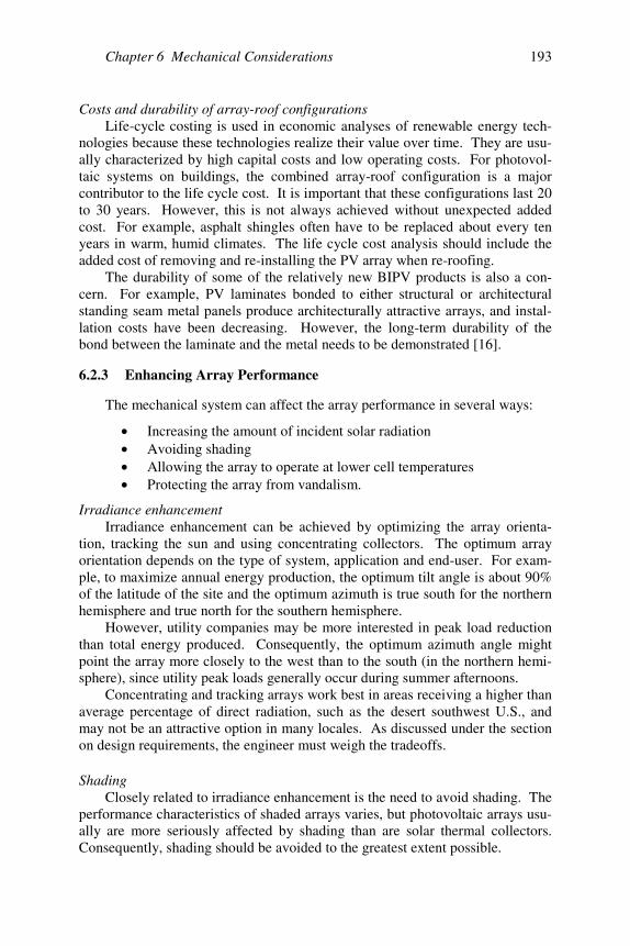
Chapter 6 Mechanical Considerations 193
Costs and durability of array-roof configurationsLife-cycle costing is used in economic analyses of renewable energy tech-
nologies because these technologies realize their value over time. They are usu-ally characterized by high capital costs and low operating costs. For photovol-taic systems on buildings, the combined array-roof configuration is a majorcontributor to the life cycle cost. It is important that these configurations last 20to 30 years. However, this is not always achieved without unexpected addedcost. For example, asphalt shingles often have to be replaced about every tenyears in warm, humid climates. The life cycle cost analysis should include theadded cost of removing and re-installing the PV array when re-roofing.
The durability of some of the relatively new BIPV products is also a con-cern. For example, PV laminates bonded to either structural or architecturalstanding seam metal panels produce architecturally attractive arrays, and instal-lation costs have been decreasing. However, the long-term durability of thebond between the laminate and the metal needs to be demonstrated [16].
6.2.3 Enhancing Array Performance
The mechanical system can affect the array performance in several ways:
• Increasing the amount of incident solar radiation• Avoiding shading• Allowing the array to operate at lower cell temperatures• Protecting the array from vandalism.
Irradiance enhancementIrradiance enhancement can be achieved by optimizing the array orienta-
tion, tracking the sun and using concentrating collectors. The optimum arrayorientation depends on the type of system, application and end-user. For exam-ple, to maximize annual energy production, the optimum tilt angle is about 90%of the latitude of the site and the optimum azimuth is true south for the northernhemisphere and true north for the southern hemisphere.
However, utility companies may be more interested in peak load reductionthan total energy produced. Consequently, the optimum azimuth angle mightpoint the array more closely to the west than to the south (in the northern hemi-sphere), since utility peak loads generally occur during summer afternoons.
Concentrating and tracking arrays work best in areas receiving a higher thanaverage percentage of direct radiation, such as the desert southwest U.S., andmay not be an attractive option in many locales. As discussed under the sectionon design requirements, the engineer must weigh the tradeoffs.
ShadingClosely related to irradiance enhancement is the need to avoid shading. The
performance characteristics of shaded arrays varies, but photovoltaic arrays usu-ally are more seriously affected by shading than are solar thermal collectors.Consequently, shading should be avoided to the greatest extent possible.
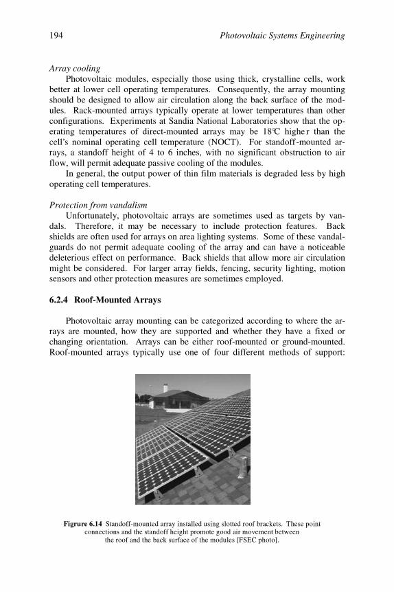
Photovoltaic Systems Engineering194
Array coolingPhotovoltaic modules, especially those using thick, crystalline cells, work
better at lower cell operating temperatures. Consequently, the array mountingshould be designed to allow air circulation along the back surface of the mod-ules. Rack-mounted arrays typically operate at lower temperatures than otherconfigurations. Experiments at Sandia National Laboratories show that the op-erating temperatures of direct-mounted arrays may be 18°C highe r than thecell’s nominal operating cell temperature (NOCT). For standoff-mounted ar-rays, a standoff height of 4 to 6 inches, with no significant obstruction to airflow, will permit adequate passive cooling of the modules.
In general, the output power of thin film materials is degraded less by highoperating cell temperatures.
Protection from vandalismUnfortunately, photovoltaic arrays are sometimes used as targets by van-
dals. Therefore, it may be necessary to include protection features. Backshields are often used for arrays on area lighting systems. Some of these vandal-guards do not permit adequate cooling of the array and can have a noticeabledeleterious effect on performance. Back shields that allow more air circulationmight be considered. For larger array fields, fencing, security lighting, motionsensors and other protection measures are sometimes employed.
6.2.4 Roof-Mounted Arrays
Photovoltaic array mounting can be categorized according to where the ar-rays are mounted, how they are supported and whether they have a fixed orchanging orientation. Arrays can be either roof-mounted or ground-mounted.Roof-mounted arrays typically use one of four different methods of support:
Figrure 6.14 Standoff-mounted array installed using slotted roof brackets. These point connections and the standoff height promote good air movement between
the roof and the back surface of the modules [FSEC photo].

Chapter 6 Mechanical Considerations 195
rack, standoff, integrated or direct. With the surge of interest in photovoltaicand building applications, better designs for each of these four roof mountingapproaches are being pursued.
Standoff MountingStandoff arrays are mounted above and parallel to the roof surface as illus-
trated in Figure 6.14. Standoff mounts work well for buildings with slopingroofs. When installing a standoff-mounted array, the photovoltaic panels orsubarrays are often attached to the roof using point connections usually at ornear the corners of the panels or subarrays. As a minimum, the standoff heightbetween the roof and the bottom of the module frame should be at least threeinches. Four to six inches is preferable. Lag screws that penetrate the roof raft-ers three to four inches may be used to fasten the mounting brackets to the roof.Spanner and J-bolt attachments, as shown in Figure 6.15, are stronger than lagbolts or lag screws and are commonly used in areas exposed to high winds.
To promote passive cooling of standoff arrays, the engineer should considerthe following designs:
• Designs that allow both lateral and vertical airflow along the back sur-face of the modules
• Designs that induce pressure differences between air inlet and exit re-gions
• Arrays with larger lateral dimensions than vertical dimensions (i.e.,higher aspect ratios).
Rack MountingRack-mounted arrays are above and tilted with respect to the roof, as illus-
trated in Figure 6.16. Rack mounts work well on flat roofs and roofs with aslope of 2 in 12 or less. They may be mechanically attached to the buildingstructure or may employ ballast to resist wind and other mechanical loads. Rackmounts are usually subjected to higher structural loads, incur higher costs formounting hardware and are often less attractive than standoff mounts. However,
Figure 6.15 Spanner and J-bolt attachments provide secure anchors for roof-mounted arrays.
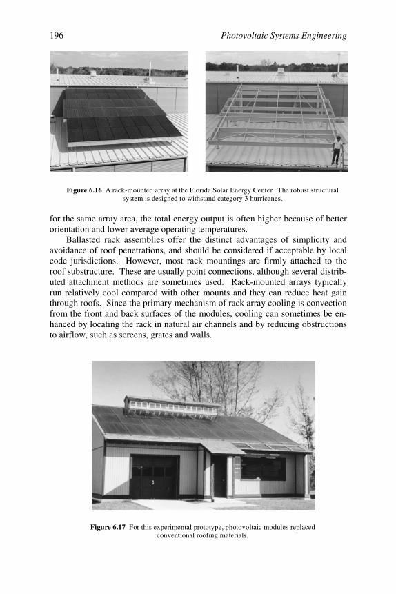
Photovoltaic Systems Engineering196
for the same array area, the total energy output is often higher because of betterorientation and lower average operating temperatures.
Ballasted rack assemblies offer the distinct advantages of simplicity andavoidance of roof penetrations, and should be considered if acceptable by localcode jurisdictions. However, most rack mountings are firmly attached to theroof substructure. These are usually point connections, although several distrib-uted attachment methods are sometimes used. Rack-mounted arrays typicallyrun relatively cool compared with other mounts and they can reduce heat gainthrough roofs. Since the primary mechanism of rack array cooling is convectionfrom the front and back surfaces of the modules, cooling can sometimes be en-hanced by locating the rack in natural air channels and by reducing obstructionsto airflow, such as screens, grates and walls.
Figure 6.16 A rack-mounted array at the Florida Solar Energy Center. The robust structuralsystem is designed to withstand category 3 hurricanes.
Figure 6.17 For this experimental prototype, photovoltaic modules replacedconventional roofing materials.

Chapter 6 Mechanical Considerations 197
Integrated MountingFor integrated arrays, also referred to as building-integrated photovoltaics
(BIPV) or integral mounting, the array replaces conventional roofing or glazingmaterials as illustrated in Figure 6.17. Because integrated arrays replace con-ventional roofing and glazing materials, they become a significant architecturalfeature of a building and can be aesthetically very pleasing.
Dimensional tolerances may be tighter for some integrated arrays than forstandoff or rack mounts. If commercial curtain-wall glazing techniques areused, larger modules are preferable to smaller modules.
Direct MountingIn direct mounting, the array is affixed directly to the roofing material
or underlayment, with little or no airspace between the module and roof. Figure6.18 illustrates a direct-mounted solar shingle.
Array operating temperatures for direct mounts are usually higher than forother mounting techniques. The use of direct mounting may become increas-ingly popular for new thin-film products that are not as sensitive to operatingtemperature. Some photovoltaic materials, such as solar shingles, fall into boththe direct and BIPV mounting categories.
6.6.5 Ground-Mounted Arrays
Ground-mounted arrays are supported by racks, poles or tracking stands.These arrays are secured to the ground to resist uplifting caused by wind loads.All ground-mounted arrays run relatively cool because good airflow is possibleover both the front and back surfaces of the modules. This cooling can be en-hanced by minimizing obstructions to airflow such as shrubbery and fences.
Figure 6.18 The solar shingle is installed directly on the roofing underlayment, with noair circulation below the PV laminate. It is one of a variety of new products
that replaces conventional roofing materials.
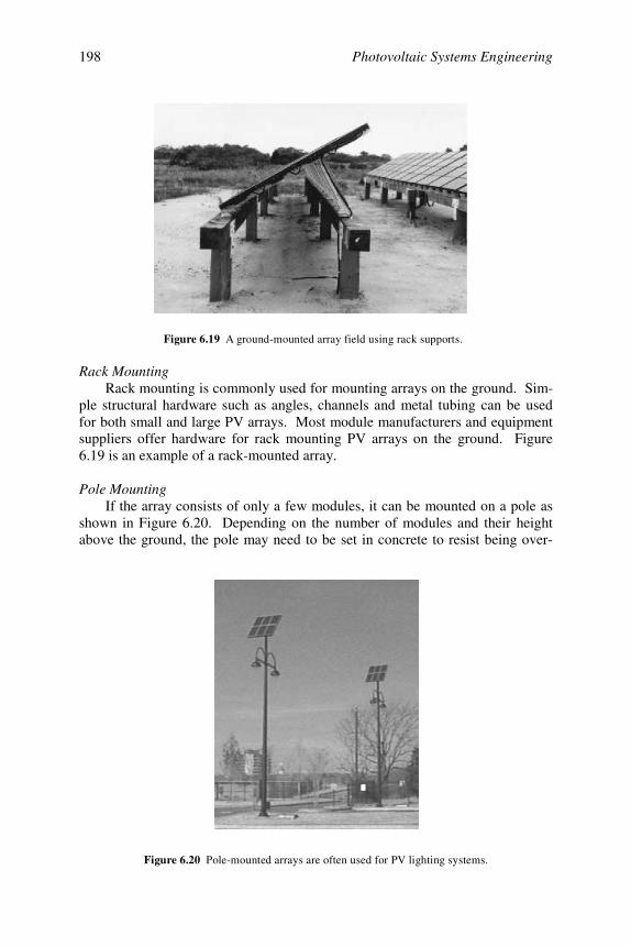
Photovoltaic Systems Engineering198
Rack MountingRack mounting is commonly used for mounting arrays on the ground. Sim-
ple structural hardware such as angles, channels and metal tubing can be usedfor both small and large PV arrays. Most module manufacturers and equipmentsuppliers offer hardware for rack mounting PV arrays on the ground. Figure6.19 is an example of a rack-mounted array.
Pole MountingIf the array consists of only a few modules, it can be mounted on a pole as
shown in Figure 6.20. Depending on the number of modules and their heightabove the ground, the pole may need to be set in concrete to resist being over-
Figure 6.19 A ground-mounted array field using rack supports.
Figure 6.20 Pole-mounted arrays are often used for PV lighting systems.
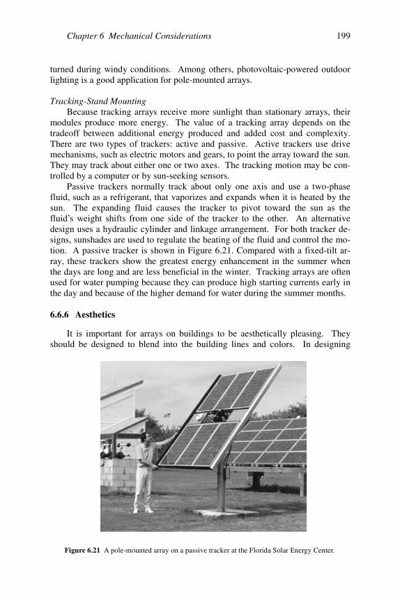
Chapter 6 Mechanical Considerations 199
turned during windy conditions. Among others, photovoltaic-powered outdoorlighting is a good application for pole-mounted arrays.
Tracking-Stand MountingBecause tracking arrays receive more sunlight than stationary arrays, their
modules produce more energy. The value of a tracking array depends on thetradeoff between additional energy produced and added cost and complexity.There are two types of trackers: active and passive. Active trackers use drivemechanisms, such as electric motors and gears, to point the array toward the sun.They may track about either one or two axes. The tracking motion may be con-trolled by a computer or by sun-seeking sensors.
Passive trackers normally track about only one axis and use a two-phasefluid, such as a refrigerant, that vaporizes and expands when it is heated by thesun. The expanding fluid causes the tracker to pivot toward the sun as thefluid’s weight shifts from one side of the tracker to the other. An alternativedesign uses a hydraulic cylinder and linkage arrangement. For both tracker de-signs, sunshades are used to regulate the heating of the fluid and control the mo-tion. A passive tracker is shown in Figure 6.21. Compared with a fixed-tilt ar-ray, these trackers show the greatest energy enhancement in the summer whenthe days are long and are less beneficial in the winter. Tracking arrays are oftenused for water pumping because they can produce high starting currents early inthe day and because of the higher demand for water during the summer months.
6.6.6 Aesthetics
It is important for arrays on buildings to be aesthetically pleasing. Theyshould be designed to blend into the building lines and colors. In designing
Figure 6.21 A pole-mounted array on a passive tracker at the Florida Solar Energy Center.

Photovoltaic Systems Engineering200
photovoltaic arrays for building applications, the architect and engineer shouldconsider the following suggestions:
• Mounting the array parallel to the roof (if appropriate)• Using the roof dimensions to establish the array aspect ratio• Avoiding harsh contrasts and patterns• Making the mounting hardware as inconspicuous as possible• Avoiding shading, even if appearance suffers somewhat.
As mentioned previously, many of the new building-integrated photovoltaicproducts add to the architectural attractiveness of buildings.
6.1 Computing Mechanical Loads and Stresses
6.1.1 Introduction
As indicated previously, the photovoltaic array is subjected to a wide varietyof mechanical influences that affect the stresses and strains in the modules,structural support members and attachment hardware. These include dead-weight loads, live loads, wind loads, and snow and ice loads. In this section, weassume a pressure distribution on the array and discuss the methods used to cal-culate its effects on critical elements of the support structure.
6.1.2 Withdrawal Loads
A high percentage of standoff-mounted photovoltaic arrays are attached tothe roof using lag screws or bolts. The lag screw typically passes through a holein a mounting bracket, possibly a mounting pad, shingles, waterproof mem-brane, sheathing and, finally, into the truss, spanner or other primary structuralwood support member. The withdrawal strength of this and other attachmentpoints is a function of the diameter of the lag screw, the length of thread embed-ded in the primary structural wood support, and the specific gravity of the wood.The allowable withdrawal load of lag screws and bolts per inch of embeddedthread is given by [3]:
2/34/3 GD800,1p = (6.13)
where: p = allowable withdrawal load (lb./in.)D = shank diameter of lag screw or bolt (in.)G = specific gravity of oven-dry wood
Values for p computed using (6.13) include a safety factor of 4.5. This rela-tively high value provides added protection just in case the actual wood usedmay have reduced strength due to variations in specific gravity, knots, grainirregularities, holes and other defects [17].
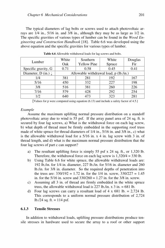
Chapter 6 Mechanical Considerations 201
The typical diameters of lag bolts or screws used to attach photovoltaic ar-rays are 1/4 in., 5/16 in. and 3/8 in., although they may be as large as 1/2 in.The specific gravities of various types of lumber can be found in the Wood En-gineering and Construction Handbook [18]. Table 6.6 was developed using theabove equation and the specific gravities for various types of lumber.
Table 6.6 Allowable withdrawal loads for lag screws and bolts.
LumberWhiteOak
SouthernYellow Pine
WhiteSpruce
DouglasFir
Specific gravity, G 0.71 0.58 0.45 0.41Diameter, D (in.) Allowable withdrawal load, p (lb./in.)
1/4 381 281 192 1675/16 450 332 227 1983/8 516 381 260 226
7/16 579 428 292 2541/2 640 473 323 281
[Values for p were computed using equation (6.13) and include a safety factor of 4.5.]
ExampleAssume the maximum uplifting normal pressure distribution on a standoff
photovoltaic array due to wind is 55 psf. If the array panel area of 24 sq. ft. issecured by four lag screws, a) What is the withdrawal force on each lag screw,b) what depth of thread must be firmly embedded in the supporting roof trussmade of white spruce for thread diameters of 1/4 in., 5/16 in. and 3/8 in., c) whatis the allowable withdrawal load for a 5/16 in. x 4 in. lag screw with 3 in. ofthread length, and d) what is the maximum normal pressure distribution that thefour lag screws of part c can support?
a) The resultant uplifting force is simply 55 psf x 24 sq. ft., or 1,320 lb.Therefore, the withdrawal force on each lag screw is 1,320/4 = 330 lb.
b) Using Table 6.6 for white spruce, the allowable withdrawal loads are:192 lb./in. for 1/4 in. diameter, 227 lb./in. for 5/16 in. diameter and 260lb./in. for 3/8 in. diameter. So the required depths of penetration intothe truss are: 330/192 = 1.72 in. for the 1/4 in. screw, 330/227 = 1.45in. for the 5/16 in. screw and 330/260 = 1.27 in. for the 3/8 in. screw.
c) Assuming all 3 in. of thread are firmly embedded in the white sprucetruss, the allowable withdrawal load is 227 lb./in. x 3 in. = 681 lb.
d) Four lag screws can carry a resultant load of 4 x 681 lb. = 2,724 lb.This corresponds to a uniform normal pressure distribution of 2,724lb./24 sq. ft. = 114 psf.
6.1.3 Tensile Stresses
In addition to withdrawal loads, uplifting pressure distributions produce ten-sile stresses in hardware used to secure the array to a roof or other support
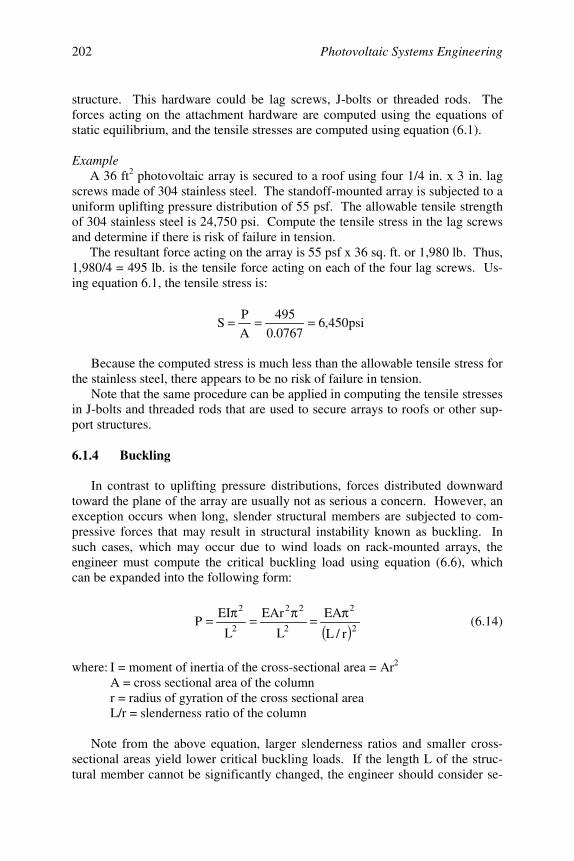
Photovoltaic Systems Engineering202
structure. This hardware could be lag screws, J-bolts or threaded rods. Theforces acting on the attachment hardware are computed using the equations ofstatic equilibrium, and the tensile stresses are computed using equation (6.1).
ExampleA 36 ft2 photovoltaic array is secured to a roof using four 1/4 in. x 3 in. lag
screws made of 304 stainless steel. The standoff-mounted array is subjected to auniform uplifting pressure distribution of 55 psf. The allowable tensile strengthof 304 stainless steel is 24,750 psi. Compute the tensile stress in the lag screwsand determine if there is risk of failure in tension.
The resultant force acting on the array is 55 psf x 36 sq. ft. or 1,980 lb. Thus,1,980/4 = 495 lb. is the tensile force acting on each of the four lag screws. Us-ing equation 6.1, the tensile stress is:
psi450,60767.0495
AP
S ===
Because the computed stress is much less than the allowable tensile stress forthe stainless steel, there appears to be no risk of failure in tension.
Note that the same procedure can be applied in computing the tensile stressesin J-bolts and threaded rods that are used to secure arrays to roofs or other sup-port structures.
6.1.4 Buckling
In contrast to uplifting pressure distributions, forces distributed downwardtoward the plane of the array are usually not as serious a concern. However, anexception occurs when long, slender structural members are subjected to com-pressive forces that may result in structural instability known as buckling. Insuch cases, which may occur due to wind loads on rack-mounted arrays, theengineer must compute the critical buckling load using equation (6.6), whichcan be expanded into the following form:
( ) 2
2
2
22
2
2
r/L
EA
L
EAr
L
EIP
π=π=π= (6.14)
where: I = moment of inertia of the cross-sectional area = Ar2
A = cross sectional area of the columnr = radius of gyration of the cross sectional areaL/r = slenderness ratio of the column
Note from the above equation, larger slenderness ratios and smaller cross-sectional areas yield lower critical buckling loads. If the length L of the struc-tural member cannot be significantly changed, the engineer should consider se-
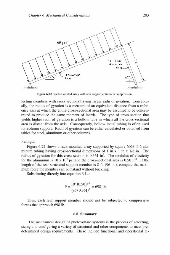
Chapter 6 Mechanical Considerations 203
lecting members with cross sections having larger radii of gyration. Conceptu-ally, the radius of gyration is a measure of an equivalent distance from a refer-ence axis at which the entire cross-sectional area may be assumed to be concen-trated to produce the same moment of inertia. The type of cross section thatyields higher radii of gyration is a hollow tube in which all the cross-sectionalarea is distant from the axis. Consequently, hollow metal tubing is often usedfor column support. Radii of gyration can be either calculated or obtained fromtables for steel, aluminum or other columns.
ExampleFigure 6.22 shows a rack-mounted array supported by square 6063 T-6 alu-
minum tubing having cross-sectional dimensions of 1 in x 1 in x 1/8 in. Theradius of gyration for this cross section is 0.361 in2. The modulus of elasticityfor the aluminum is 10 x 106 psi and the cross-sectional area is 0.50 in2. If thelength of the rear structural support member is 8 ft. (96 in.), compute the maxi-mum force the member can withstand without buckling.
Substituting directly into equation 6.14:
( )( )
698361.0/96
50.010P
2
27
=π= lb.
Thus, each rear support member should not be subjected to compressiveforces that approach 698 lb.
6.8 Summary
The mechanical design of photovoltaic systems is the process of selecting,sizing and configuring a variety of structural and other components to meet pre-determined design requirements. These include functional and operational re-
Figure 6.22 Rack-mounted array with rear support column in compression.
2
2
3KRWRYROWDLF$UUD\
µ[µ[µ$OXPLQXP
7XELQJ
IW

Photovoltaic Systems Engineering204
quirements and design constraints. Meeting the design requirements under pre-vailing constraints requires a weighing of alternatives and trade-offs.
The engineer must determine the mechanical forces acting on the array andselect the proper materials and structural members to safely carry these loads.Photovoltaic mechanical design requires knowledge of materials, mechanics,structures and the characteristics of photovoltaic systems.
Standards, when incorporated into building codes, establish the guidelinesfor designing and installing photovoltaic systems.
The American Society of Civil Engineers publishes standards on designloads for buildings and other structures. These standards can be applied to solararrays. The greatest mechanical loading on photovoltaic arrays and structures isthe result of aerodynamic forces from wind. ASCE specifies the different windspeeds that should be used for design throughout the U.S.
The array mounting design should provide adequate access to the sun’s ra-diation and allow the photovoltaic modules to operate at acceptable cell tem-peratures. The array should also be sufficiently accessible for installation andmaintenance and aesthetically appropriate for the site and application.
Problems
6.1 Consider the following facts concerning a steel alloy and aluminum alloy:a) steel is stronger, b) steel is stiffer and c) aluminum stretches much morethan steel. Sketch the stress-strain curves for both on the same stress-straingraph (see Figure 6.3). Show the relative positions of the yield strength,ultimate strength and rupture strength. Also, indicate on the graphs howthe moduli of elasticity compare for steel and aluminum.
6.2 For two bars having cross sectional areas A1 = 0.25 in2 and A2 = 25 in2,subjected to uniform axial forces P1 = 100 lb and P2 = 1000 lb, computethe uniform stresses in each bar.
6.3 During a simple pull test of a bar, the deformation per unit length wasmeasured at 0.000167 in/in. The corresponding stress was 5000 psi. Fur-ther in the test, the elongation per unit length and corresponding stresswere 0.000667 in/in and 20,000 psi. If the proportional limit is 30,000 psi,what is the modulus of elasticity? Would this result be valid if the propor-tional limit was 18,000 psi? Explain.
6.4 A uniform bar has length = L and cross sectional area = A. Rather than aforce P acting on the end of the bar, the only force is the uniformly distrib-uted weight of the bar. If the total weight of the bar is W, show that thetotal elongation is δ = WL/2AE. If its weight per unit volume is w, alsoshow that δ = wL2/2E.

Chapter 6 Mechanical Considerations 205
6.5 A steel bar having a cross sectional area of 0.5 in2 and a length L = 600 ftis suspended vertically. The force P acting on the lower end is 5000 lb. Ifsteel weighs 490 lb/ft3 and E = 30 x 106 psi, find the elongation of the bar.(Hint: Use the results of Problem 6.4.)
6.6 A photovoltaic array is to be mounted on the roof of a nursing home,which is adjacent to a hospital. It is located in the Topeka, KS, area and issubjected to high wind loading. List at least three possible functional re-quirements and three operational requirements. Also identify four con-straints the designer must consider. Identify the trade-offs that might beweighed.
6.7 Why are building codes that affect the mechanical and structural design ofphotovoltaic systems much less uniform throughout the U.S. than electricalcodes? Explain.
6.8 Give two examples of cases when the design loading for the photovoltaicarray and structural supports is not dominated by wind loading.
6.9 What conditions must be satisfied before Bernoulli’s equation can be usedto relate the pressure and velocity between two points in the flow field?Does a photovoltaic array meet these conditions? Explain. Why is an un-derstanding of the Bernoulli relationship important when considering windloading on photovoltaic systems?
6.10 The design wind load calculation involves the product of the wind speed, aforce coefficient and an importance factor. How is the design wind speeddetermined? If the force coefficient (i.e., fudge factor) cannot be derivedanalytically, how might it be determined experimentally? The importancefactor is related to the consequences of failure the greater the conse-quences, the higher the factor. How would the importance factor for a PVsystem on a rural home compare with the application in Problem 6.6?
6.11 List four objectives in designing an array mounting system.
6.12 For a fixed-orientation array to be mounted on a south-facing roof, discussthe advantages and disadvantages of each of the four roof-mounting con-figurations.
6.13 12.8 x 10⁻⁶ per oF and E = 10 x 106 psi. The initial temperature at whichthere are no stresses is 59oF, and the final temperature is 200oF. All otherdimensions, properties and information are the same as in the example forFigure 6.5. Compute the stresses in both the stainless steel bolt and thealuminum sleeve at 200oF.

Photovoltaic Systems Engineering206
6.14 Four lag screws of 5/16 in. diameter and 3.5 in. length are used to attach an8 ft by 8 ft standoff array to an asphalt shingle roof. The total threadlength is 2.5 in. and the combined thickness of the mounting bracket, pad,shingles, roof membrane and plywood sheathing is 1.0 in. If the lag screwpenetrates into the roof truss made of Southern yellow pine, what is theallowable withdrawal load on each lag screw? What is the maximum up-lift loading in psf that the array can withstand?
6.15 A four-module photovoltaic array has an area of 40 sq. ft. and will be se-cured using six mounting brackets. Each bracket uses two 5/16 in. lagscrews to secure the standoff-mounted array. The roof trusses are made ofwhite spruce. The design wind load is 55 psf. What is the minimumthread penetration for each fastener?
6.16 A standoff-mounted array has a surface area of 50 sq. ft. and is secured toan asphalt shingle roof with four steel J-bolts of 3/8 in. diameter. If theallowable tensile stress for the steel is 40,000 psi, are the J-bolts of suffi-cient strength to carry a maximum uplifting wind load of 65 psf? What isthe factor of safety?
6.17 An array of four photovoltaic modules, each with an area of 10 sq. ft., is tobe mounted above and parallel to a standing seam metal roof using 6 L-brackets. The modules themselves can withstand a load of 75 psf. If it isdesired to support the 75 psf uplifting load on the full array with one lagscrew in each bracket, and if each bracket has an allowable withdrawal re-sistance of 300 lb./in., what is the minimum thread length that must pene-trate the roof truss?
6.18 Assume the ratio of direct to total irradiance is the same for two differentlocations, one at 30o north latitude and one at 60o north latitude. Which lo-cation would benefit the most from a two-axis tracking array (versus afixed-orientation array)? Explain.
6.19 For more effective cooling of standoff-mounted photovoltaic arrays, wouldyou recommend higher or lower aspect ratios? Explain.
6.20 A rack-mounted array similar to the one in Figure 6.22 is supported at therear by two 4-ft. columns of 6063 T-6 aluminum tubing. The modulus ofelasticity of the aluminum is 10 x 106 psi. The cross-sectional area is 0.5in2 and the radius of gyration is 0.361 in. What is the moment of inertia ofthe cross sectional area in units of in.4? Compute the critical bucklingload, P.
Chapter 6 Mechanical Considerations 207
References
[1] Dieter, G. E., Engineering Design: A Materials and Processing Approach, 2nd Ed.,McGraw-Hill, New York, 1991.
[2] Hanks, R. W., Materials Science Engineering: An Introduction, Harcourt, Brace &World, New York, 1970.
[3] Avallone, E. A. and Baumeister, T., Eds., Marks’ Standard Handbook for Mechani-cal Engineers, 10th Ed., McGraw-Hill, New York, 1996.
[4] Kutz, M., Mechanical Engineers’ Handbook , 2nd Ed., John Wiley & Sons, NewYork, 1998.
[5] Singer, F. L., Strength of Materials, 2nd Ed., Harper & Brothers Publishers, NewYork, 1962.
[6] Clauser, H. R., Editor-in-Chief, The Encyclopedia of Engineering Materials andProcesses, Reinhold Publishing, New York, 1963.
[7] Larson, W. J. and Wertz, J. R., Space Mission Analysis and Design, 2nd Ed., Micro-cosm, Inc. and Kluwer Academic Publishers, Torrance, CA, 1992.
[8] Minimum Design Loads for Buildings and Other Structures, ASCE Standard,SEI/ASCE 7–02, Revision of ASCE 7-98, American Society of Civil Engineers,Reston, VA, 2003.
[9] Bertin, J. J. and Smith, M. L., Aerodynamics for Engineers, 2nd Ed., Prentice Hall,Englewood Cliffs, NJ, 1989.
[10] Hurt, H. H., Aerodynamics for Naval Aviators, Navweps 00-80T-80, U.S. Navy,1960.
[11] Modular Photovoltaic Array Field, prepared for Sandia National Laboratories,SAND83-7028, Hughes Aircraft Company, 1984.
[12] Miller, R. D. and Zimmerman, D. K., Wind Loads on Flat Plate Photovoltaic ArrayFields, Phase II Final Report, prepared for Jet Propulsion Laboratory, Contract No.NAS-7-100-954833, Boeing Engineering and Construction Company, Seattle, WA,1979.
[13] Marion, B. and Atmaram, G., Preliminary Design of a 15– 25 kWp Thin-Film Photo-voltaic System, prepared for the U.S. Department of Energy, Florida Solar EnergyCenter, Cape Canaveral, FL, November 13, 1987.
[14] Wind Design of Flat Panel Photovoltaic Array Structures, prepared for Sandia Na-tional Laboratories, SAND79–7057, Bechtel National, Inc., June 1980.
[15] Miller, R. D. and Zimmerman, D. K., Wind Loads on Flat Plate Photovoltaic ArrayFields, Phase III and Phase IV Final Reports, prepared for Jet Propulsion Labora-tory, Contract No. NAS–7–100–954833, Boeing Engineering and Con structionCompany, Seattle, WA, April 1981.
[16] Ventre, G.G., A Program Plan for Photovoltaic Buildings in Florida, prepared forthe Florida Energy Office/Department of Community Affairs and Sandia NationalLaboratories, Florida Solar Energy Center, Cocoa, FL, FSEC–PD–2 5–99, January1999.
[17] Wood Handbook—Wood as an Engineering Material , U. S. Department of Agricul-ture, Forest Service, Forest Products Laboratory, Madison, WI, 1999.
[18] Faherty, K.F. and Williamson, T.G., Wood Engineering and Construction Hand-book, 3rd Ed., McGraw-Hill, New York, 1997.

Photovoltaic Systems Engineering208
Suggested Reading
Building Integrated Photovoltaic Project in the 21st Century Townhouses, AdvancedHousing Technology Program, National Association of Home Builders ResearchCenter, Inc., Upper Marlboro, MD, June 1997.
Epstein, S. G., Aluminum and Its Alloys, Aluminum Association, Inc., presented atthe Annual Liberty Bell Corrosion Course, sponsored by the National Associa-tion of Corrosion Engineers, Washington, D.C., September 1978.
Healey, H., An Investigation of the Feasibility of a National Structural CertificationProcess, Contract Report for the Solar Rating and Certification Corporation,Healey and Associates, Merritt Island, FL, September 25, 1998.
Hollister, S. C., The Engineering Interpretation of Weather Bureau Records forWind Loading on Structures, National Bureau of Standards, Washington, D.C.,November 1970.
IEEE Recommended Practice for Qualification of Photovoltaic (PV) Modules, IEEEStandard 1262–1995, IEEE Standards Coordinating Committee 21 on Photovol-taics, Institute of Electrical and Electronics Engineers, Inc., New York, April 12,1996.
Manual of Steel Construction, 8th Ed., American Institute of Steel Construction,Chicago, 1980.
McCluney, W. R., Introduction to Radiometry and Photometry, Artech House, Inc.,Norwood, MA, 1994.
Mehta, K. C. and Marshall, R. D., Guide to the Use of the Wind Load Provisions ofASCE 7– 95, ASCE Press, Reston, VA, 1998.
Metal Roofing, Roofer Magazine, July 1997.Orlowski, H., Corrosion protection for solar systems: methods of eliminating an old
problem applied to solar components, Heat/Piping/Air Conditioning, July 1976.Photovoltaic System Design, Course Manual, Florida Solar Energy Center, Cocoa,
FL, FSEC-GP–31–86, April 1996.Post, H. N., Low cost structures for photovoltaic arrays, Proc. 14th IEEE Photovol-
taic Specialists Conference, San Diego, CA, January 7–10, 1980.Post, H. N. and Noel, G. T., A comparative evaluation of new low-cost array field
designs for grid-connected photovoltaic systems, Proc. 19th Intersociety EnergyConversion Engineering Conference, San Francisco, CA, August 19–24, 1984.
Roark, R. J., Formulas for Stress and Strain, McGraw-Hill, New York, 1954.Russell, M. C. and Kern, E. C., Stand-Off Building Block Systems for Roof-Mounted
Photovoltaic Arrays, Sandia Contract 58–8796, Massachusetts Institute of Tech-nology, December 1985.
Shigley, J. E. and Mischke, C. R., Mechanical Engineering Design, 5th Ed.,McGraw-Hill , New York, 1989.
Sick, F. and Erge, T., Eds., Photovoltaics in Buildings: A Design Handbook for Ar-chitects and Engineers, International Energy Agency, Paris, 1996.
Smith, W. F., Principles of Materials Science and Engineering, 2nd Ed., McGraw-Hill, New York, 1990.
Stefanakos, E. K. et al., Effect of row-to-row shading on the output of flat platesouth facing photovoltaic arrays, Solar Engineering−1986 , American Society ofMechanical Engineers, Anaheim, CA, April 13–16, 1986.
The Design of Residential Photovoltaic Systems, SAND87–1951, PhotovoltaicSystem Design Assistance Center, Sandia National Laboratories, Albuquerque,NM, December 1988.
209
Chapter 7STAND-ALONE PV SYSTEMS
7.1 Introduction
This chapter will introduce the design process for several complete self-contained PV systems. For each system, a life-cycle cost analysis will be madefor several design options to illustrate the iterative process that leads to reason-able system cost effectiveness. The first system will be a relatively simple re-frigeration system, except that the system will be designed to meet a criticalneed. The second system will be another mountain cabin. In this chapter, thecomplete cabin system will be designed, including consideration of placement ofthe various loads and computation of the wire sizes needed to meet the needs ofthe loads. A hybrid residence will then be designed, with an emphasis on theprocess of selecting an appropriate mix of PV and propane electrical generation.This residence will use 120 V loads as opposed to the 24 V loads of the cabinand will thus require an inverter and a more interesting control system.
In any design, the first task is normally to determine the load. Often there areseveral choices. For example, a choice might be made between an inexpensiveincandescent lamp and a more expensive fluorescent lamp. In the first exampleof this chapter, a comparison will be made among systems that use two differenttypes of refrigerators. One uses a relatively inexpensive, but somewhat ineffi-cient, unit. The other uses a more expensive, but more efficient, unit.
The load voltage, current and power are needed for proper sizing of fuses,wires, batteries and other system components. In some cases, not all these quan-tities are given. For example, the specifications for a refrigerator may only givethe voltage and kWh per month, or Ah per day. In these cases, it may be neces-sary to either calculate or estimate the other parameters.
Once the load has been determined, then the amount of battery backup needsto be determined. Some systems will not need batteries, some will have minimalstorage and some will require sufficient battery storage to meet critical perform-ance requirements in which the system must operate more than 99% of the time.It will also be the responsibility of the engineer to determine whether to use bat-teries that require maintenance or to use maintenance-free batteries at nearlytwice the initial cost.
After battery selection, the size of the PV array must be determined. Thenthe electronic components of the system, such as charge controllers and invertersare selected. Finally, the balance of system components are selected, includingthe array mounts, the wiring, switches, fuses, battery compartments, lightningprotection and, perhaps, monitoring instrumentation.
As the design process is completed for each of the following systems, generaldesign guidelines will be presented for later use. While computer programs maybe available for system design, emphasis in this chapter will instead be placed onsound, common-sense reasoning and the use of good engineering judgment.

Photovoltaic Systems Engineering210
In order to keep the design examples as realistic as possible, many of thesystem components described in the examples of this chapter have been found onan assortment of web sites. It is important for the reader to note that the pre-sumed use of a particular component or web site in an example does not consti-tute an endorsement of the component or the company. Vendors and componentavailability change on a daily basis, so when a real system is designed, the de-signer should carry out an extensive search for the components that best meet thedesign goals. Hopefully the procedures for component selection outlined in thischapter will prove to be useful when the opportunity to design a real system pre-sents itself.
7.2 A Critical Need Refrigeration System
7.2.1 Design Specifications
It is desired to provide electric power for 10 cubic feet of refrigeration forstorage of medication. The medication is costly and difficult to obtain, so thesystem must have 99% availability. The system will be located in a village inAngola where villagers will be able to keep a careful watch on system perform-ance so any problems will become immediately evident.
7.2.2 Design Implementation
Two implementations will be explored concurrently. The first will use astandard, 10-cubic-foot, 120 V ac refrigerator. The second will use a 10-cubic-foot, high-efficiency 24 V dc refrigerator. The ac refrigerator costs $338 andconsumes 530 kWh per year. The dc refrigerator costs $1515 and uses 12.5 Ahper day at 90oF, with an operating current of 2.3 A at 24 V. An ac refrigeratorthat costs $1900 and uses 24 Ah per day is also available, but, since it wouldrequire an inverter that would increase the overall cost beyond the dc unit thatuses slightly less energy per day, it will not be considered in this example [1].
Load DeterminationThe first task is to determine relevant parameters for comparing the units.
Since the battery capacity will be determined in Ah, it makes sense to determinethe load energy requirements in Ah. Multiplication by voltage gives actual en-ergy in Wh for the purist who notices that Ah are not proper units for energy.
To convert 530 kWh per year to Ah per day, simply divide by 365 to getkWh per day, then multiply by 1000 to get Wh per day. Finally, since the refrig-erator will be supplied by an inverter with a 24 V input, dividing by 24 yields theAh per day. However, since the inverter is used, the inverter efficiency must beaccounted for by dividing the Ah per day by the inverter efficiency. Except forpure sine inverters, most modern inverters will operate at close to 95% effi-ciency. Using a conservative 90% figure, the daily energy use of the ac refrig-erator is determined to be 67.2 Ah per day.
Chapter 7 Stand-Alone PV Systems 211
At this point, it should be noted that there are energy losses in the systemwiring. The National Electrical Code requires that overall voltage drop in asystem be less than 5%. A well-designed PV system, however, will keep voltagedrop in the 2% range, since the added cost of wire is nearly always less than thecost of additional PV modules to supply power lost in wiring.
Determination of Average Daily PV System Load
1. Identify all loads to be connected to the PV system.2. For each load, determine its voltage, current, power and daily operat-
ing hours. For some loads, the operation may vary on a daily, monthlyor seasonal basis. If so, this must be accounted for in calculating dailyaverages.
3. Separate ac loads from dc loads.4. Determine average daily Ah for each load from current and operating
hours data. If operating hours differ from day to day during the week,the daily average over the week should be calculated. If average dailyoperating hours vary from month to month, then the load calculationmay need to be determined for each month.
5. Add up the Ah for the dc loads, being sure all are at the same voltage.6. If some dc loads are at a different voltage, which will require a dc-to-
dc converter, then the converter input Ah for these loads needs to ac-count for the conversion efficiency of the converter.
7. For ac loads, the dc input current to the inverter must be determinedand the dc Ah are then determined from the dc input current. The dcinput current is determined by equating the ac load power to the dc in-put power and then dividing by the efficiency of the inverter.
8. Add the Ah for the dc loads to the Ah for the ac loads, then divide bythe wire efficiency factor and the battery efficiency factor to obtain thecorrected average daily Ah for the total load.
9. The total ac load power will determine the required size of theinverter. Individual load powers will be needed to determine wiresizing to the loads. Total load current will be compared with total ar-ray current when sizing wire from battery to controller.
The power lost in the wiring is determined by the product of the current andthe voltage drop. Depending on the nature of the load, a drop in voltage mayresult in either a drop or a rise in current. Normally the current will dropslightly, but, in some motors with constant loads, the current will rise. If the loadis an MPT, the current will also rise if the voltage drops. However, for a voltagedrop of only 2%, it is reasonable to assume the load current will remain essen-tially constant. With this assumption, the power loss can be approximated by theproduct of load current at nominal load voltage and the voltage drop. Hence, a2% voltage drop implies a 2% power loss, or, in terms of Ah, a 2% Ah loss.This loss must be added to the PV array power output requirements. Thus, a 2%
Photovoltaic Systems Engineering212
voltage drop implies a wiring efficiency of 98%, and the load Ah per day mustbe increased by dividing by 0.98 to account for the wiring loss.
Finally, if a system contains battery storage, the losses encountered incharging and discharging the batteries must be accounted for. As long as thebatteries are not discharged or charged at a rate higher than rated by the manu-facturer for full capacity performance, a 10% loss for charge and discharge is areasonable default choice. This means the system load must be divided by 0.9 toaccount for the additional energy loss in the batteries. Of course, for a systemwithout batteries, this factor need not be applied.
In the present case, to account for wiring and battery losses, the correctedload daily energy use becomes 67.2 ÷ 0.98 ÷ 0.9 = 76.2 Ah/day for the ac refrig-erator system. For the dc refrigerator system, the corrected load becomes12.5 ÷ 0.98 ÷ 0.9 = 14.2 Ah/day. Note that the corrected load is the Ah that mustbe supplied to the batteries so the batteries can power the connected load, as-suming batteries are used.
Battery SelectionIn Chapter 3 it was observed that the number of days of autonomy required
for critical need applications depends on the location of the system. In locationswith relatively high average insolation, even during the worst part of the year,less storage is needed. The number of days of autonomy required for critical andnoncritical system performance is tabulated for some locations [2]. If the mini-mum peak sun hours over the period of operation of the load is known for a lo-cation, the number of days of autonomy can be estimated from the followingformulas from Chapter 3:
3.18T9.1D mincrit +−= (7.1a)
or58.4T48.0D minnon +−= . (7.1b)
where Tmin is the minimum peak sun hours for the selected system collector tiltduring any month of operation and D represents the number of storage days re-quired, either for critical or noncritical storage. Note that these formulas areonly valid for minimum peak sun hours of about one hour per day. Obviously ifthe sun does not shine, more than 18.3 days of storage will be needed if the sys-tem is to run more than 18.3 days.
Annual peak sun hours for selected locations are given in Appendix A. Re-ferring to the table for Luanda, Angola, it is evident that the best annual arrayperformance is obtained with the array tilted at the latitude (8.82o south). Notethat, in the Southern Hemisphere, this means the array faces north with a tilt of8.82° above horizontal. This gives an average daily peak sun hours of 5.03 overthe year. With this tilt, the minimum peak sun hours of 3.71 occurs in July. Theminimum peak sun hours for the latitude–15 o tilt (see problem 7.1) is 3.36 inJuly, and the minimum peak sun hours for the latitude+15o tilt is 3.93 in July. A
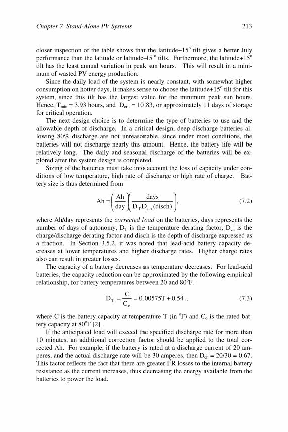
Chapter 7 Stand-Alone PV Systems 213
closer inspection of the table shows that the latitude+15o tilt gives a better Julyperformance than the latitude or latitude–15 o tilts. Furthermore, the latitude+15o
tilt has the least annual variation in peak sun hours. This will result in a mini-mum of wasted PV energy production.
Since the daily load of the system is nearly constant, with somewhat higherconsumption on hotter days, it makes sense to choose the latitude+15o tilt for thissystem, since this tilt has the largest value for the minimum peak sun hours.Hence, Tmin = 3.93 hours, and Dcrit = 10.83, or approximately 11 days of storagefor critical operation.
The next design choice is to determine the type of batteries to use and theallowable depth of discharge. In a critical design, deep discharge batteries al-lowing 80% discharge are not unreasonable, since under most conditions, thebatteries will not discharge nearly this amount. Hence, the battery life will berelatively long. The daily and seasonal discharge of the batteries will be ex-plored after the system design is completed.
Sizing of the batteries must take into account the loss of capacity under con-ditions of low temperature, high rate of discharge or high rate of charge. Bat-tery size is thus determined from
=
)disch(DD
days
day
AhAh
chT
, (7.2)
where Ah/day represents the corrected load on the batteries, days represents thenumber of days of autonomy, DT is the temperature derating factor, Dch is thecharge/discharge derating factor and disch is the depth of discharge expressed asa fraction. In Section 3.5.2, it was noted that lead-acid battery capacity de-creases at lower temperatures and higher discharge rates. Higher charge ratesalso can result in greater losses.
The capacity of a battery decreases as temperature decreases. For lead-acidbatteries, the capacity reduction can be approximated by the following empiricalrelationship, for battery temperatures between 20 and 80oF.
54.0T00575.0CC
Do
T +== , (7.3)
where C is the battery capacity at temperature T (in oF) and Co is the rated bat-tery capacity at 80oF [2].
If the anticipated load will exceed the specified discharge rate for more than10 minutes, an additional correction factor should be applied to the total cor-rected Ah. For example, if the battery is rated at a discharge current of 20 am-peres, and the actual discharge rate will be 30 amperes, then Dch = 20/30 = 0.67.This factor reflects the fact that there are greater I2R losses to the internal batteryresistance as the current increases, thus decreasing the energy available from thebatteries to power the load.

Photovoltaic Systems Engineering214
If the battery charge rate exceeds the rated charge rate, an alternate calcula-tion of battery capacity should be performed and compared with (7.2). Lead-acid batteries are typically designed to take 10 hours from zero charge to fullcharge. Hence, if 10 hours times the PV charging rate in amperes exceeds thebattery capacity in Ah calculated in (7.2), it means the PV array is capable offully charging the batteries in less than 10 hours. If this condition should occur,the battery capacity should be determined by the product of the rated chargingtime and the available charging current, rather than by (7.2).
In the present case, the battery capacity required would be 14.2 × 11 ÷ 0.8 =195 Ah for the dc refrigerator and would be 76.2 × 11 ÷ 0.8 = 1048 Ah for the acrefrigerator, assuming unity values for DT and Dch and (disch) = 0.8. Neithersituation has a charging rate that will charge the batteries in less than 10 hours ora load that will discharge the batteries in less than 10 hours.
Once the battery capacity is determined, the number of batteries in parallelrequired for the system is determined by dividing the total capacity required bythe capacity of a single battery. Normally this computation will result in a non-integral quantity. The system designer must then decide whether to round up, toround down or to use a different battery. When the system voltage requires bat-teries to be connected in series as well as in parallel, rounding up or down willinvolve more than one battery. For example, in a 48 V system, rounding up willshow a need for 4 additional 12 V batteries or 8 additional 6 V batteries. Theround-up or round-down decision should thus be made carefully.
The judgment as to whether to round up or to round down should be influ-enced by knowledge as to whether the user of the loads can cut back on use dur-ing cloudy periods to conserve battery charge. Another factor that will influ-ence judgment is whether at least a small amount of charging can be anticipatedduring periods of prolonged overcast. Professional judgment by a qualified,experienced engineer in these situations may result in savings in system cost overa system for which a computer has made the decision using unknown criteriahidden somewhere in the program. Many good PV system sizing programs areavailable, but the final system should always be checked by the design engineerto be sure it makes good technical and economic sense.
Batteries come in many shapes, sizes and types. Probably the first decisionto make when specifying batteries is whether the owner is capable of maintainingthe batteries, since maintenance-free batteries are nearly twice as expensive asflooded lead-acid batteries that require periodic testing and watering. One par-ticular battery is a 6 V, 350 Ah flooded lead-acid unit that costs $198 and has alife expectancy of 5 to 8 years. To obtain 195 Ah storage at 24 volts requiresfour of these batteries, at a cost of $792. To obtain 1048 Ah of storage at 24volts would require 12 of these batteries, at a cost of $2376.
Another of the many available batteries is a 6 V, 220 Ah flooded lead-acid,deep-discharge, golf cart battery that sells for $85 and has a 5-year life expec-tancy. For the 195 Ah system, four batteries are required at a cost of $340. For
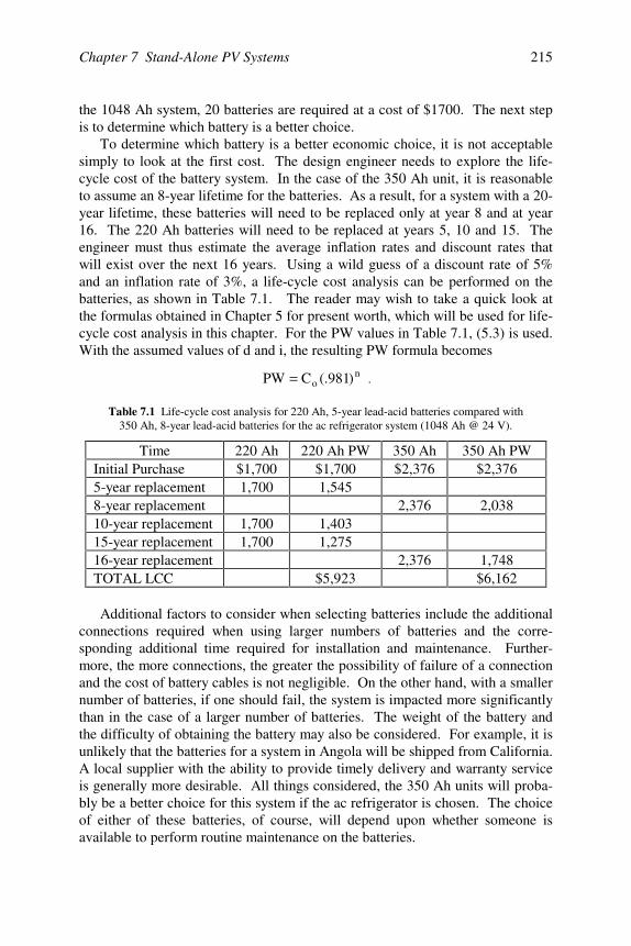
Chapter 7 Stand-Alone PV Systems 215
the 1048 Ah system, 20 batteries are required at a cost of $1700. The next stepis to determine which battery is a better choice.
To determine which battery is a better economic choice, it is not acceptablesimply to look at the first cost. The design engineer needs to explore the life-cycle cost of the battery system. In the case of the 350 Ah unit, it is reasonableto assume an 8-year lifetime for the batteries. As a result, for a system with a 20-year lifetime, these batteries will need to be replaced only at year 8 and at year16. The 220 Ah batteries will need to be replaced at years 5, 10 and 15. Theengineer must thus estimate the average inflation rates and discount rates thatwill exist over the next 16 years. Using a wild guess of a discount rate of 5%and an inflation rate of 3%, a life-cycle cost analysis can be performed on thebatteries, as shown in Table 7.1. The reader may wish to take a quick look atthe formulas obtained in Chapter 5 for present worth, which will be used for life-cycle cost analysis in this chapter. For the PW values in Table 7.1, (5.3) is used.With the assumed values of d and i, the resulting PW formula becomes
no )981(.CPW = .
Table 7.1 Life-cycle cost analysis for 220 Ah, 5-year lead-acid batteries compared with350 Ah, 8-year lead-acid batteries for the ac refrigerator system (1048 Ah @ 24 V).
Time 220 Ah 220 Ah PW 350 Ah 350 Ah PWInitial Purchase $1,700 $1,700 $2,376 $2,3765-year replacement 1,700 1,545 8-year replacement 2,376 2,03810-year replacement 1,700 1,403 15-year replacement 1,700 1,275 16-year replacement 2,376 1,748TOTAL LCC $5,923 $6,162
Additional factors to consider when selecting batteries include the additionalconnections required when using larger numbers of batteries and the corre-sponding additional time required for installation and maintenance. Further-more, the more connections, the greater the possibility of failure of a connectionand the cost of battery cables is not negligible. On the other hand, with a smallernumber of batteries, if one should fail, the system is impacted more significantlythan in the case of a larger number of batteries. The weight of the battery andthe difficulty of obtaining the battery may also be considered. For example, it isunlikely that the batteries for a system in Angola will be shipped from California.A local supplier with the ability to provide timely delivery and warranty serviceis generally more desirable. All things considered, the 350 Ah units will proba-bly be a better choice for this system if the ac refrigerator is chosen. The choiceof either of these batteries, of course, will depend upon whether someone isavailable to perform routine maintenance on the batteries.
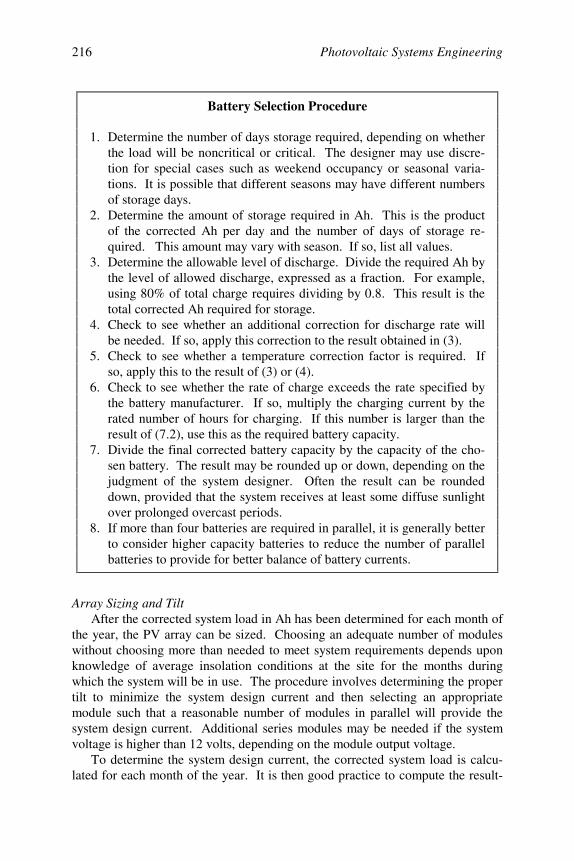
Photovoltaic Systems Engineering216
Battery Selection Procedure
1. Determine the number of days storage required, depending on whetherthe load will be noncritical or critical. The designer may use discre-tion for special cases such as weekend occupancy or seasonal varia-tions. It is possible that different seasons may have different numbersof storage days.
2. Determine the amount of storage required in Ah. This is the productof the corrected Ah per day and the number of days of storage re-quired. This amount may vary with season. If so, list all values.
3. Determine the allowable level of discharge. Divide the required Ah bythe level of allowed discharge, expressed as a fraction. For example,using 80% of total charge requires dividing by 0.8. This result is thetotal corrected Ah required for storage.
4. Check to see whether an additional correction for discharge rate willbe needed. If so, apply this correction to the result obtained in (3).
5. Check to see whether a temperature correction factor is required. Ifso, apply this to the result of (3) or (4).
6. Check to see whether the rate of charge exceeds the rate specified bythe battery manufacturer. If so, multiply the charging current by therated number of hours for charging. If this number is larger than theresult of (7.2), use this as the required battery capacity.
7. Divide the final corrected battery capacity by the capacity of the cho-sen battery. The result may be rounded up or down, depending on thejudgment of the system designer. Often the result can be roundeddown, provided that the system receives at least some diffuse sunlightover prolonged overcast periods.
8. If more than four batteries are required in parallel, it is generally betterto consider higher capacity batteries to reduce the number of parallelbatteries to provide for better balance of battery currents.
Array Sizing and TiltAfter the corrected system load in Ah has been determined for each month of
the year, the PV array can be sized. Choosing an adequate number of moduleswithout choosing more than needed to meet system requirements depends uponknowledge of average insolation conditions at the site for the months duringwhich the system will be in use. The procedure involves determining the propertilt to minimize the system design current and then selecting an appropriatemodule such that a reasonable number of modules in parallel will provide thesystem design current. Additional series modules may be needed if the systemvoltage is higher than 12 volts, depending on the module output voltage.
To determine the system design current, the corrected system load is calcu-lated for each month of the year. It is then good practice to compute the result-
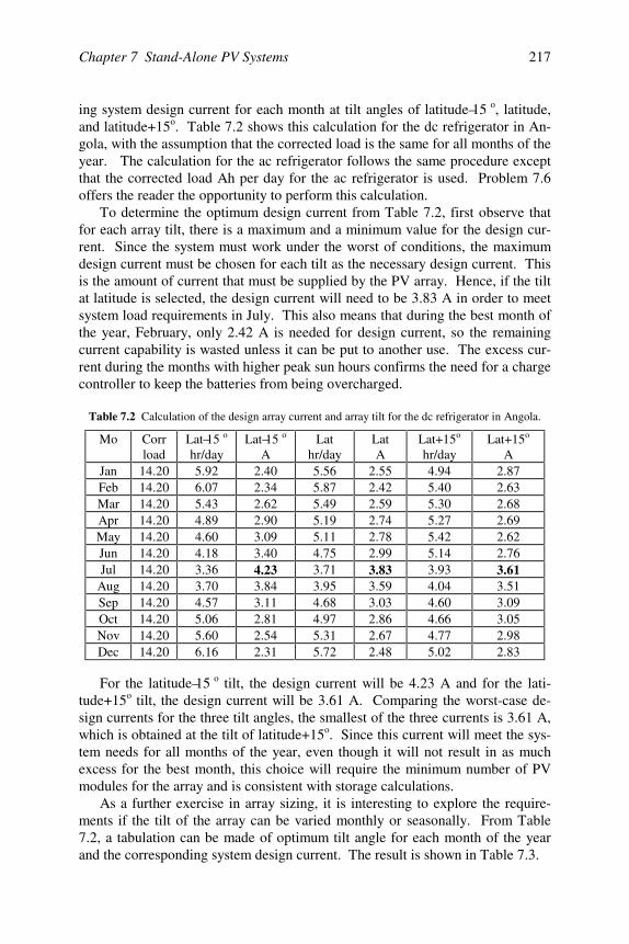
Chapter 7 Stand-Alone PV Systems 217
ing system design current for each month at tilt angles of latitude–15 o, latitude,and latitude+15o. Table 7.2 shows this calculation for the dc refrigerator in An-gola, with the assumption that the corrected load is the same for all months of theyear. The calculation for the ac refrigerator follows the same procedure exceptthat the corrected load Ah per day for the ac refrigerator is used. Problem 7.6offers the reader the opportunity to perform this calculation.
To determine the optimum design current from Table 7.2, first observe thatfor each array tilt, there is a maximum and a minimum value for the design cur-rent. Since the system must work under the worst of conditions, the maximumdesign current must be chosen for each tilt as the necessary design current. Thisis the amount of current that must be supplied by the PV array. Hence, if the tiltat latitude is selected, the design current will need to be 3.83 A in order to meetsystem load requirements in July. This also means that during the best month ofthe year, February, only 2.42 A is needed for design current, so the remainingcurrent capability is wasted unless it can be put to another use. The excess cur-rent during the months with higher peak sun hours confirms the need for a chargecontroller to keep the batteries from being overcharged.
Table 7.2 Calculation of the design array current and array tilt for the dc refrigerator in Angola.
Mo Corrload
Lat–15 o
hr/dayLat–15 o
ALat
hr/dayLatA
Lat+15o
hr/dayLat+15o
AJan 14.20 5.92 2.40 5.56 2.55 4.94 2.87Feb 14.20 6.07 2.34 5.87 2.42 5.40 2.63Mar 14.20 5.43 2.62 5.49 2.59 5.30 2.68Apr 14.20 4.89 2.90 5.19 2.74 5.27 2.69May 14.20 4.60 3.09 5.11 2.78 5.42 2.62Jun 14.20 4.18 3.40 4.75 2.99 5.14 2.76Jul 14.20 3.36 4.23 3.71 3.83 3.93 3.61
Aug 14.20 3.70 3.84 3.95 3.59 4.04 3.51Sep 14.20 4.57 3.11 4.68 3.03 4.60 3.09Oct 14.20 5.06 2.81 4.97 2.86 4.66 3.05Nov 14.20 5.60 2.54 5.31 2.67 4.77 2.98Dec 14.20 6.16 2.31 5.72 2.48 5.02 2.83
For the latitude–15 o tilt, the design current will be 4.23 A and for the lati-tude+15o tilt, the design current will be 3.61 A. Comparing the worst-case de-sign currents for the three tilt angles, the smallest of the three currents is 3.61 A,which is obtained at the tilt of latitude+15o. Since this current will meet the sys-tem needs for all months of the year, even though it will not result in as muchexcess for the best month, this choice will require the minimum number of PVmodules for the array and is consistent with storage calculations.
As a further exercise in array sizing, it is interesting to explore the require-ments if the tilt of the array can be varied monthly or seasonally. From Table7.2, a tabulation can be made of optimum tilt angle for each month of the yearand the corresponding system design current. The result is shown in Table 7.3.
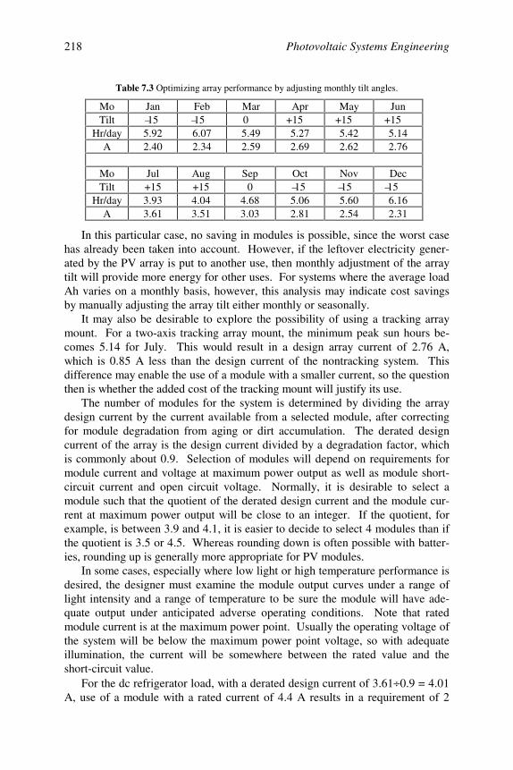
Photovoltaic Systems Engineering218
Table 7.3 Optimizing array performance by adjusting monthly tilt angles.
Mo Jan Feb Mar Apr May JunTilt –15 –15 0 +15 +15 +15
Hr/day 5.92 6.07 5.49 5.27 5.42 5.14A 2.40 2.34 2.59 2.69 2.62 2.76
Mo Jul Aug Sep Oct Nov DecTilt +15 +15 0 –15 –15 –15
Hr/day 3.93 4.04 4.68 5.06 5.60 6.16A 3.61 3.51 3.03 2.81 2.54 2.31
In this particular case, no saving in modules is possible, since the worst casehas already been taken into account. However, if the leftover electricity gener-ated by the PV array is put to another use, then monthly adjustment of the arraytilt will provide more energy for other uses. For systems where the average loadAh varies on a monthly basis, however, this analysis may indicate cost savingsby manually adjusting the array tilt either monthly or seasonally.
It may also be desirable to explore the possibility of using a tracking arraymount. For a two-axis tracking array mount, the minimum peak sun hours be-comes 5.14 for July. This would result in a design array current of 2.76 A,which is 0.85 A less than the design current of the nontracking system. Thisdifference may enable the use of a module with a smaller current, so the questionthen is whether the added cost of the tracking mount will justify its use.
The number of modules for the system is determined by dividing the arraydesign current by the current available from a selected module, after correctingfor module degradation from aging or dirt accumulation. The derated designcurrent of the array is the design current divided by a degradation factor, whichis commonly about 0.9. Selection of modules will depend on requirements formodule current and voltage at maximum power output as well as module short-circuit current and open circuit voltage. Normally, it is desirable to select amodule such that the quotient of the derated design current and the module cur-rent at maximum power output will be close to an integer. If the quotient, forexample, is between 3.9 and 4.1, it is easier to decide to select 4 modules than ifthe quotient is 3.5 or 4.5. Whereas rounding down is often possible with batter-ies, rounding up is generally more appropriate for PV modules.
In some cases, especially where low light or high temperature performance isdesired, the designer must examine the module output curves under a range oflight intensity and a range of temperature to be sure the module will have ade-quate output under anticipated adverse operating conditions. Note that ratedmodule current is at the maximum power point. Usually the operating voltage ofthe system will be below the maximum power point voltage, so with adequateillumination, the current will be somewhere between the rated value and theshort-circuit value.
For the dc refrigerator load, with a derated design current of 3.61 ÷ 0.9 = 4.01A, use of a module with a rated current of 4.4 A results in a requirement of 2
Chapter 7 Stand-Alone PV Systems 219
modules in series. For the dc refrigerator with two-axis tracking array mount,the derated design current is 2.76 ÷ 0.9 = 3.07 A, or 2 modules in series, usingmodules rated at 50 W maximum power each.
The ac refrigerator, on the other hand, ends up with a fixed array designcurrent of 76.2 ÷ 3.61 = 21.1 A, which leads to a derated design current of 23.5 A.Using the 4.4 A modules in a fixed array results in the need for 10.66 modules,which rounds up to 12 modules—6 parallel sets of 2 series modul es.
From a first cost perspective, if the cost of a 4.4 A module is listed as $350,the array cost for the dc refrigerator with no tracking is $700. If the cost of the3.07 A module is $250, then the array cost for the tracking configuration is $500.For the ac nontracking case, the array cost is $4200, assuming the use of 4.4 Amodules in the array.
Array Sizing and Tilt Procedure
1. Determine the design current for each month of the year by dividingthe corrected Ah load for the system each month by the monthly aver-age peak sun hours at each array tilt angle.
2. Determine the worst-case (highest monthly) design current for each tiltangle.
3. For a fixed mount, select the tilt angle that results in the lowest worst-case design current.
4. If tracking mounts are considered, then determine the design currentfor one- and two-axis trackers. Note that the one-axis tracker tracksfrom east to west and needs to have its design currents checked for thethree angles of fixed trackers.
5. Determine the derated array current by dividing the design current bythe module derating factor.
6. Select a module that meets the illumination and temperature require-ments of the system as well as having a rated output current and volt-age at maximum power consistent with system needs.
7. Determine the number of modules in parallel by dividing the deratedarray current by the rated module current. Round up or down asdeemed appropriate.
8. Determine the number of modules in series by dividing the nominalsystem voltage by the lowest anticipated module voltage of a modulesupplying power to the system. In this case, it is almost always neces-sary to round up.
9. The total number of modules is the product of the number in paralleland the number in series.
The cost of a mount for 2 modules is about $200, while a mount for 12 mod-ules is approximately $600. A two-axis tracking mount for 2 modules will cost
Photovoltaic Systems Engineering220
approximately $500. The overall first cost of array plus mount is thus relativelyclose for the dc refrigerator case. The choice becomes contingent on the judg-ment of the engineer as to whether the nontracking system or the tracking systemwill be more reliable over the life of the system.
Controller, Inverter and/or dc:dc Converter SelectionThe dc refrigerator will require a battery charge controller as a part of the
system and the ac refrigerator will require both controller and inverter to 120 Vac. Selection of any of these components is affected by the number of bells andwhistles the designer feels the item should have. Many of these optional featureswere discussed in Chapter 3.
In the present case, relatively simple controllers are preferred because com-plexity sometimes leads to reliability problems. The controller must be capableof handling the battery charging current from the array as well as the current tothe load. Inverters and converters need to be able to handle starting/surge cur-rents of the loads they service. In this case, the dc refrigerator system will workfine with a simple $100 controller, whereas the ac system will require a largercontroller at a cost closer to $200.
For a motor-driven appliance, the designer must determine whether the motorwill be damaged by dc or by harmonics. Each can cause heating of the motorabove its rated operating temperature. If so, the inverter must be selected tohave dc and harmonic content below the limits allowed by the motor. The costof a suitable inverter for the ac refrigerator will be about $125.
Wire, Fuse and Switch SelectionProper wire sizing depends on the current to be carried by the wire, but, at
low voltages, primarily on the length of the wire and the resulting voltage drop.It is generally useful to lay out the system and then tabulate the lengths of thevarious wire runs along with the allowable voltage drops. This enables a simplecalculation of the required resistance per 1000 feet of wire to keep the wire volt-age drop within allowable limits. Once the resistance per 1000 feet is known,the proper wire size can be selected. The correct wire size is the larger of eitherthe size needed to carry the rated current or the size needed to meet system volt-age drop constraints.
To determine wire sizes for the array, it is necessary to recognize that undercertain unusual conditions, it is possible for the reflection from cloud to focusthe sunlight on an array. This phenomenon requires that the wire be able to carrythe array current as enhanced by cloud focusing. To allow for cloud focusing,the array short-circuit current is multiplied by 1.25 to obtain the maximum cur-rent from array to controller. This maximum array current is then multiplied byanother factor of 1.25, as required by the NEC for continuous operation, andwire sizes are then chosen to meet this ampacity requirement. The wiring of PVsource circuits and PV output circuits must thus be capable of carrying 156% ofthe short-circuit current of either the source circuit or output circuit, whichever is
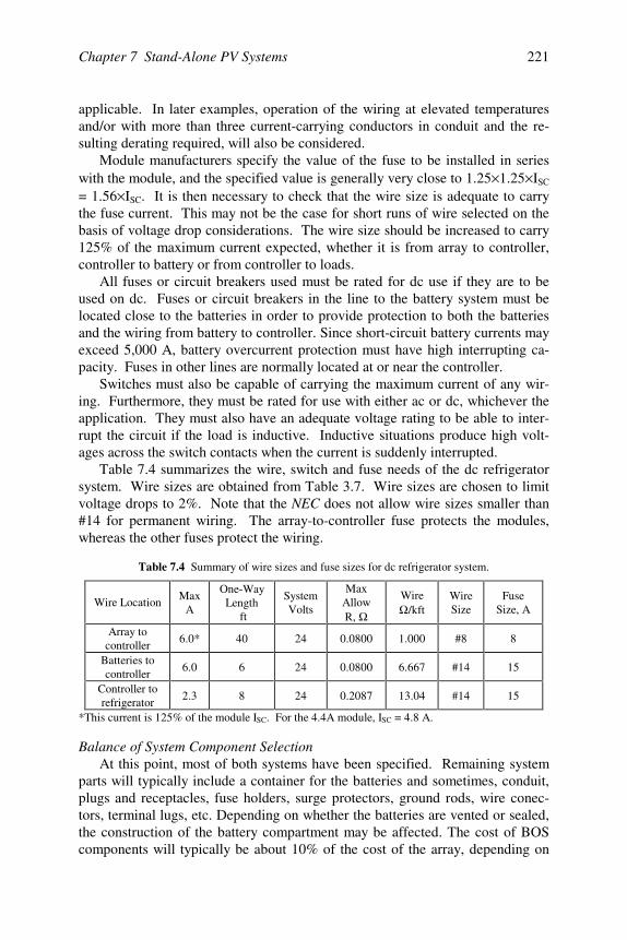
Chapter 7 Stand-Alone PV Systems 221
applicable. In later examples, operation of the wiring at elevated temperaturesand/or with more than three current-carrying conductors in conduit and the re-sulting derating required, will also be considered.
Module manufacturers specify the value of the fuse to be installed in serieswith the module, and the specified value is generally very close to 1.25 × 1.25 × ISC
= 1.56 × ISC. It is then necessary to check that the wire size is adequate to carrythe fuse current. This may not be the case for short runs of wire selected on thebasis of voltage drop considerations. The wire size should be increased to carry125% of the maximum current expected, whether it is from array to controller,controller to battery or from controller to loads.
All fuses or circuit breakers used must be rated for dc use if they are to beused on dc. Fuses or circuit breakers in the line to the battery system must belocated close to the batteries in order to provide protection to both the batteriesand the wiring from battery to controller. Since short-circuit battery currents mayexceed 5,000 A, battery overcurrent protection must have high interrupting ca-pacity. Fuses in other lines are normally located at or near the controller.
Switches must also be capable of carrying the maximum current of any wir-ing. Furthermore, they must be rated for use with either ac or dc, whichever theapplication. They must also have an adequate voltage rating to be able to inter-rupt the circuit if the load is inductive. Inductive situations produce high volt-ages across the switch contacts when the current is suddenly interrupted.
Table 7.4 summarizes the wire, switch and fuse needs of the dc refrigeratorsystem. Wire sizes are obtained from Table 3.7. Wire sizes are chosen to limitvoltage drops to 2%. Note that the NEC does not allow wire sizes smaller than#14 for permanent wiring. The array-to-controller fuse protects the modules,whereas the other fuses protect the wiring.
Table 7.4 Summary of wire sizes and fuse sizes for dc refrigerator system.
Wire Location MaxA
One-WayLength
ft
SystemVolts
MaxAllowR, Ω
WireΩ /kft
WireSize
FuseSize, A
Array tocontroller
6.0* 40 24 0.0800 1.000 #8 8
Batteries tocontroller
6.0 6 24 0.0800 6.667 #14 15
Controller torefrigerator
2.3 8 24 0.2087 13.04 #14 15
*This current is 125% of the module ISC. For the 4.4A module, ISC = 4.8 A.
Balance of System Component SelectionAt this point, most of both systems have been specified. Remaining system
parts will typically include a container for the batteries and sometimes, conduit,plugs and receptacles, fuse holders, surge protectors, ground rods, wire conec-tors, terminal lugs, etc. Depending on whether the batteries are vented or sealed,the construction of the battery compartment may be affected. The cost of BOScomponents will typically be about 10% of the cost of the array, depending on
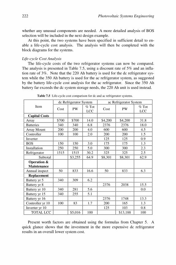
Photovoltaic Systems Engineering222
whether any unusual components are needed. A more detailed analysis of BOSselection will be included in the next design example.
At this point, the two systems have been specified in sufficient detail to en-able a life-cycle cost analysis. The analysis will then be completed with theblock diagrams for the systems.
Life-cycle Cost AnalysisThe life-cycle costs of the two refrigerator systems can now be compared.
The analysis is presented in Table 7.5, using a discount rate of 5% and an infla-tion rate of 3%. Note that the 220 Ah battery is used for the dc refrigerator sys-tem while the 350 Ah battery is used for the ac refrigerator system, as suggestedby the battery life-cycle cost analysis for the ac refrigerator. Since the 350 Ahbattery far exceeds the dc system storage needs, the 220 Ah unit is used instead.
Table 7.5 Life-cycle cost comparison for dc and ac refrigerator systems.
dc Refrigerator System ac Refrigerator SystemItem
Cost PW% TotLCC
Cost PW% TotLCC
Capital CostsArray $700 $700 14.0 $4,200 $4,200 31.8Batteries 340 340 6.8 2376 2376 18.0Array Mount 200 200 4.0 600 600 4.5Controller 100 100 2.0 200 200 1.5Inverter 125 125 0.9BOS 150 150 3.0 175 175 1.3Installation 250 250 5.0 300 300 2.3Refrigerator 1515 1515 30.2 325 325 2.5
Subtotal $3,255 64.9 $8,301 $8,301 62.9Operation &Maintenance
Annual inspect 50 833 16.6 50 833 6.3Replacement
Battery yr 5 340 309 6.2Battery yr 8 2376 2038 15.5Battery yr 10 340 281 5.6 0.0Battery yr 15 340 255 5.1Battery yr 16 2376 1748 13.3Controller yr 10 100 83 1.7 200 165 1.3Inverter yr 10 125 103 0.8
TOTAL LCC $5,016 100 $13,188 100
Present worth factors are obtained using the formulas from Chapter 5. Aquick glance shows that the investment in the more expensive dc refrigeratorresults in an overall lower system cost.
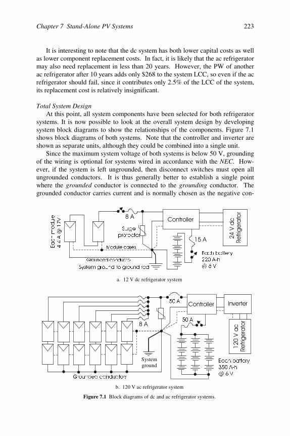
Chapter 7 Stand-Alone PV Systems 223
It is interesting to note that the dc system has both lower capital costs as wellas lower component replacement costs. In fact, it is likely that the ac refrigeratormay also need replacement in less than 20 years. However, the PW of anotherac refrigerator after 10 years adds only $268 to the system LCC, so even if the acrefrigerator should fail, since it contributes only 2.5% of the LCC of the system,its replacement cost is relatively insignificant.
Total System DesignAt this point, all system components have been selected for both refrigerator
systems. It is now possible to look at the overall system design by developingsystem block diagrams to show the relationships of the components. Figure 7.1shows block diagrams of both systems. Note that the controller and inverter areshown as separate units, although they could be combined into a single unit.
Since the maximum system voltage of both systems is below 50 V, groundingof the wiring is optional for systems wired in accordance with the NEC. How-ever, if the system is left ungrounded, then disconnect switches must open allungrounded conductors. It is thus generally better to establish a single pointwhere the grounded conductor is connected to the grounding conductor. Thegrounded conductor carries current and is normally chosen as the negative con-
a. 12 V dc refrigerator system
*URXQGHGFRQGXFWRUV
(DFKEDWWHU\
$K
#9
b. 120 V ac refrigerator system
Figure 7.1 Block diagrams of dc and ac refrigerator systems.
6XUJH
SURWHFWRU
6\VWHPJURXQGWRJURXQGURG
(DFKEDWWHU\
$K
#9
0RGXOHFDVHV
(DFKPRGXOH
$#9
*URXQGHGFRQGXFWRU
$
$
Systemground
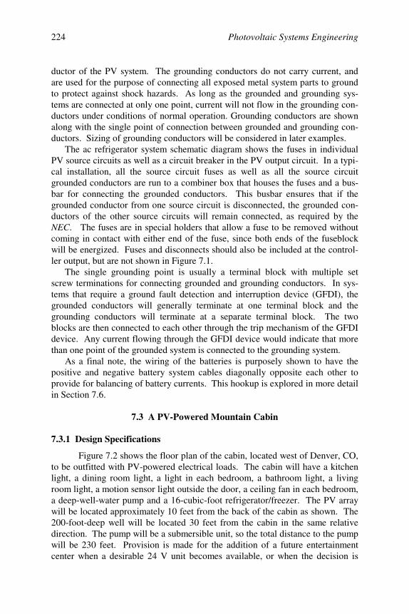
Photovoltaic Systems Engineering224
ductor of the PV system. The grounding conductors do not carry current, andare used for the purpose of connecting all exposed metal system parts to groundto protect against shock hazards. As long as the grounded and grounding sys-tems are connected at only one point, current will not flow in the grounding con-ductors under conditions of normal operation. Grounding conductors are shownalong with the single point of connection between grounded and grounding con-ductors. Sizing of grounding conductors will be considered in later examples.
The ac refrigerator system schematic diagram shows the fuses in individualPV source circuits as well as a circuit breaker in the PV output circuit. In a typi-cal installation, all the source circuit fuses as well as all the source circuitgrounded conductors are run to a combiner box that houses the fuses and a bus-bar for connecting the grounded conductors. This busbar ensures that if thegrounded conductor from one source circuit is disconnected, the grounded con-ductors of the other source circuits will remain connected, as required by theNEC. The fuses are in special holders that allow a fuse to be removed withoutcoming in contact with either end of the fuse, since both ends of the fuseblockwill be energized. Fuses and disconnects should also be included at the control-ler output, but are not shown in Figure 7.1.
The single grounding point is usually a terminal block with multiple setscrew terminations for connecting grounded and grounding conductors. In sys-tems that require a ground fault detection and interruption device (GFDI), thegrounded conductors will generally terminate at one terminal block and thegrounding conductors will terminate at a separate terminal block. The twoblocks are then connected to each other through the trip mechanism of the GFDIdevice. Any current flowing through the GFDI device would indicate that morethan one point of the grounded system is connected to the grounding system.
As a final note, the wiring of the batteries is purposely shown to have thepositive and negative battery system cables diagonally opposite each other toprovide for balancing of battery currents. This hookup is explored in more detailin Section 7.6.
7.3 A PV-Powered Mountain Cabin
7.3.1 Design Specifications
Figure 7.2 shows the floor plan of the cabin, located west of Denver, CO,to be outfitted with PV-powered electrical loads. The cabin will have a kitchenlight, a dining room light, a light in each bedroom, a bathroom light, a livingroom light, a motion sensor light outside the door, a ceiling fan in each bedroom,a deep-well-water pump and a 16-cubic-foot refrigerator/freezer. The PV arraywill be located approximately 10 feet from the back of the cabin as shown. The200-foot-deep well will be located 30 feet from the cabin in the same relativedirection. The pump will be a submersible unit, so the total distance to the pumpwill be 230 feet. Provision is made for the addition of a future entertainmentcenter when a desirable 24 V unit becomes available, or when the decision is
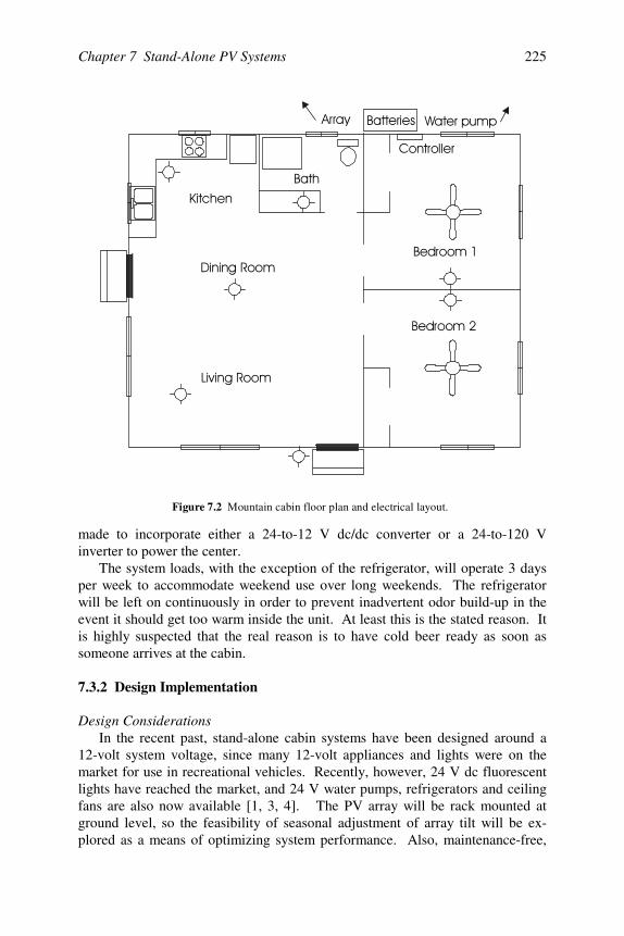
Chapter 7 Stand-Alone PV Systems 225
made to incorporate either a 24-to-12 V dc/dc converter or a 24-to-120 Vinverter to power the center.
The system loads, with the exception of the refrigerator, will operate 3 daysper week to accommodate weekend use over long weekends. The refrigeratorwill be left on continuously in order to prevent inadvertent odor build-up in theevent it should get too warm inside the unit. At least this is the stated reason. Itis highly suspected that the real reason is to have cold beer ready as soon assomeone arrives at the cabin.
7.3.2 Design Implementation
Design ConsiderationsIn the recent past, stand-alone cabin systems have been designed around a
12-volt system voltage, since many 12-volt appliances and lights were on themarket for use in recreational vehicles. Recently, however, 24 V dc fluorescentlights have reached the market, and 24 V water pumps, refrigerators and ceilingfans are also now available [1, 3, 4]. The PV array will be rack mounted atground level, so the feasibility of seasonal adjustment of array tilt will be ex-plored as a means of optimizing system performance. Also, maintenance-free,
!
"!
#
$
Figure 7.2 Mountain cabin floor plan and electrical layout.

Photovoltaic Systems Engineering226
valve-regulated lead-acid batteries will be used as a part of keeping systemmaintenance to an absolute minimum.
Load DeterminationAt this point, it should be abundantly clear that the only reasonable choice
for the refrigerator/freezer will be a high efficiency dc unit. Perusal of a dc re-frigerator vendor web site [1] leads to a 24 V unit that uses approximately 20Ah/day in the winter and 25 Ah/day in the summer at a cost of only $2419.
For the water pump, it is first necessary to determine the water needs for thecabin. This determination can be quite a wild guess unless the uses of the waterare reasonably well defined. Assuming the only means of heating water is a pro-pane stove, it is reasonable to assume that showers will not be too lengthy.However, if a solar water heater is added later, shower length may increase. Areasonable estimate for water usage might be 40 gallons per day per person, withanticipated occupancy of 4 persons. This equates to a total water requirement of160 gallons per day. If more people use the cabin, it may be necessary to dosome water rationing. In the worst case, where drinking is the only use made ofthe water, 160 people would still have a gallon each per day for drinking overthe 3-day weekend. It is assumed that less water is used in winter, spring and fallthan the 160 gallons per day of summer use.
The next step is to go to the manufacturers’ catalogs or to the internet. Forexample, [3] and [4] list a number of different water pumps. It is not likely thata low-horsepower pump at the surface of the well will be able to lift water a dis-tance of 200 feet on the suction side of the pump, even though it may be able tolift water this distance on the pressure side. For deep wells, normally a sub-mersible pump is the best choice.
The first check to make on a pump to be used in a system with battery stor-age is whether it can pump the needed water in either a day or a week. If thepump pumps the needed water in a day, then only a 160 gallon storage tank willbe needed. If it takes all week to pump the water for the weekend, then a 480gallon storage tank will be needed. The pumping power, and, hence, the voltageand current of the pump motor, will depend on the flow rate and the lift distance.If the top of the storage tank is 10 ft above ground to provide pressure for thesystem, and, allowing for 5% piping losses, the equivalent lift for the pump willbe 210 × 1.05 = 220.5 ft.
Suppose two pumps are considered. One pump will overcome a 220 ft headat 0.94 GPM when supplied with 24 V dc at a current of 4.21 A. The cost of thispump is $604. The other pump, costing $590, will pump 1.03 GPM @ 24 V dcand 3.85 A. The relative efficiencies of the two pumps can be determined bylooking at the quotient of pumping rate to power consumed, or, since both run atthe same voltage, the quotient of pumping rate and operating current. For thefirst pump, this ratio is 0.223, and for the second pump, the ratio is 0.268.Hence, from an efficiency perspective, the second pump is 20% more efficient.
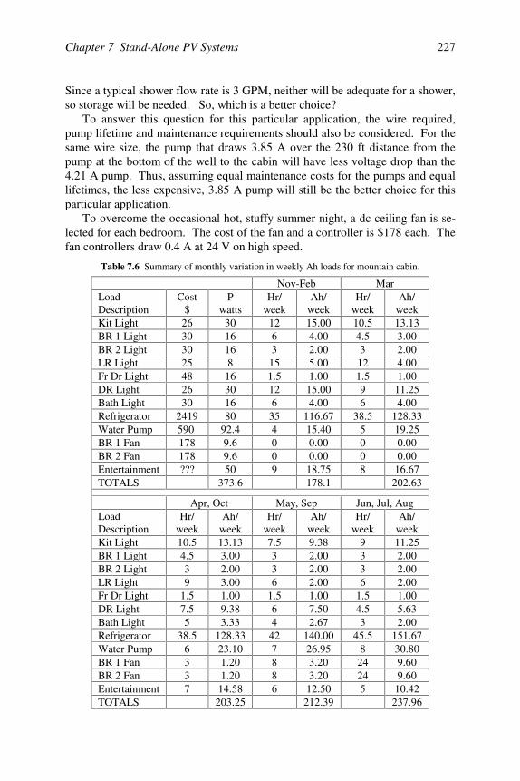
Chapter 7 Stand-Alone PV Systems 227
Since a typical shower flow rate is 3 GPM, neither will be adequate for a shower,so storage will be needed. So, which is a better choice?
To answer this question for this particular application, the wire required,pump lifetime and maintenance requirements should also be considered. For thesame wire size, the pump that draws 3.85 A over the 230 ft distance from thepump at the bottom of the well to the cabin will have less voltage drop than the4.21 A pump. Thus, assuming equal maintenance costs for the pumps and equallifetimes, the less expensive, 3.85 A pump will still be the better choice for thisparticular application.
To overcome the occasional hot, stuffy summer night, a dc ceiling fan is se-lected for each bedroom. The cost of the fan and a controller is $178 each. Thefan controllers draw 0.4 A at 24 V on high speed.
Table 7.6 Summary of monthly variation in weekly Ah loads for mountain cabin.
Nov-Feb MarLoadDescription
Cost$
Pwatts
Hr/week
Ah/week
Hr/week
Ah/week
Kit Light 26 30 12 15.00 10.5 13.13BR 1 Light 30 16 6 4.00 4.5 3.00BR 2 Light 30 16 3 2.00 3 2.00LR Light 25 8 15 5.00 12 4.00Fr Dr Light 48 16 1.5 1.00 1.5 1.00DR Light 26 30 12 15.00 9 11.25Bath Light 30 16 6 4.00 6 4.00Refrigerator 2419 80 35 116.67 38.5 128.33Water Pump 590 92.4 4 15.40 5 19.25BR 1 Fan 178 9.6 0 0.00 0 0.00BR 2 Fan 178 9.6 0 0.00 0 0.00Entertainment ??? 50 9 18.75 8 16.67TOTALS 373.6 178.1 202.63
Apr, Oct May, Sep Jun, Jul, AugLoadDescription
Hr/week
Ah/week
Hr/week
Ah/week
Hr/week
Ah/week
Kit Light 10.5 13.13 7.5 9.38 9 11.25BR 1 Light 4.5 3.00 3 2.00 3 2.00BR 2 Light 3 2.00 3 2.00 3 2.00LR Light 9 3.00 6 2.00 6 2.00Fr Dr Light 1.5 1.00 1.5 1.00 1.5 1.00DR Light 7.5 9.38 6 7.50 4.5 5.63Bath Light 5 3.33 4 2.67 3 2.00Refrigerator 38.5 128.33 42 140.00 45.5 151.67Water Pump 6 23.10 7 26.95 8 30.80BR 1 Fan 3 1.20 8 3.20 24 9.60BR 2 Fan 3 1.20 8 3.20 24 9.60Entertainment 7 14.58 6 12.50 5 10.42TOTALS 203.25 212.39 237.96
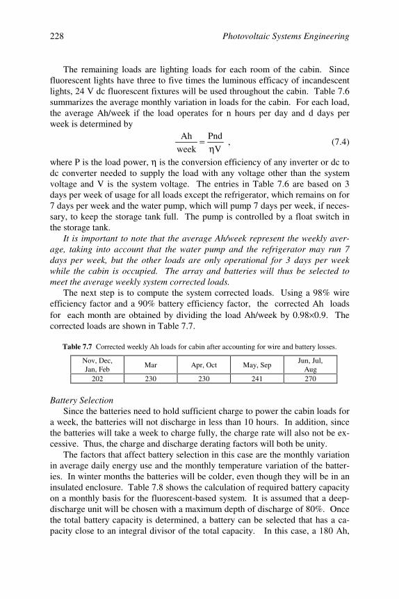
Photovoltaic Systems Engineering228
The remaining loads are lighting loads for each room of the cabin. Sincefluorescent lights have three to five times the luminous efficacy of incandescentlights, 24 V dc fluorescent fixtures will be used throughout the cabin. Table 7.6summarizes the average monthly variation in loads for the cabin. For each load,the average Ah/week if the load operates for n hours per day and d days perweek is determined by
VPnd
weekAh
η= , (7.4)
where P is the load power, η is the conversion efficiency of any inverter or dc todc converter needed to supply the load with any voltage other than the systemvoltage and V is the system voltage. The entries in Table 7.6 are based on 3days per week of usage for all loads except the refrigerator, which remains on for7 days per week and the water pump, which will pump 7 days per week, if neces-sary, to keep the storage tank full. The pump is controlled by a float switch inthe storage tank.
It is important to note that the average Ah/week represent the weekly aver-age, taking into account that the water pump and the refrigerator may run 7days per week, but the other loads are only operational for 3 days per weekwhile the cabin is occupied. The array and batteries will thus be selected tomeet the average weekly system corrected loads.
The next step is to compute the system corrected loads. Using a 98% wireefficiency factor and a 90% battery efficiency factor, the corrected Ah loadsfor each month are obtained by dividing the load Ah/week by 0.98 × 0.9. Thecorrected loads are shown in Table 7.7.
Table 7.7 Corrected weekly Ah loads for cabin after accounting for wire and battery losses.
Nov, Dec,Jan, Feb
Mar Apr, Oct May, SepJun, Jul,
Aug202 230 230 241 270
Battery SelectionSince the batteries need to hold sufficient charge to power the cabin loads for
a week, the batteries will not discharge in less than 10 hours. In addition, sincethe batteries will take a week to charge fully, the charge rate will also not be ex-cessive. Thus, the charge and discharge derating factors will both be unity.
The factors that affect battery selection in this case are the monthly variationin average daily energy use and the monthly temperature variation of the batter-ies. In winter months the batteries will be colder, even though they will be in aninsulated enclosure. Table 7.8 shows the calculation of required battery capacityon a monthly basis for the fluorescent-based system. It is assumed that a deep-discharge unit will be chosen with a maximum depth of discharge of 80%. Oncethe total battery capacity is determined, a battery can be selected that has a ca-pacity close to an integral divisor of the total capacity. In this case, a 180 Ah,
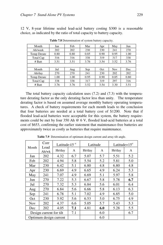
Chapter 7 Stand-Alone PV Systems 229
12 V, 8-year lifetime sealed lead-acid battery costing $300 is a reasonablechoice, as indicated by the ratio of total capacity to battery capacity.
Table 7.8 Determination of system battery capacity.
Month Jan Feb Mar Apr May JunAh/week 202 202 230 230 241 270
Temp Derate 0.80 0.80 0.85 0.90 0.95 1.00Total Cap 316 316 338 319 317 338
# Batt 3.51 3.51 3.76 3.54 3.52 3.76
Month Jul Aug Sep Oct Nov DecAh/day 270 270 241 230 202 202
Temp Derate 1.00 1.00 0.95 0.90 0.85 0.80Total Cap 338 338 317 319 297 316
# Batt 3.76 3.76 3.52 3.54 3.30 3.51
The total battery capacity calculation uses (7.2) and (7.3) with the tempera-ture derating factor as the only derating factor less than unity. The temperaturederating factor is based on assumed average monthly battery operating tempera-tures. A check of battery requirements for each month leads to the conclusionthat four batteries are needed at a total battery cost of $1200. Note that ifflooded lead-acid batteries were acceptable for this system, the battery require-ments could be met by four 350 Ah @ 6 V, flooded lead-acid batteries at a totalcost of $653, confirming the earlier statement that maintenance-free batteries areapproximately twice as costly as batteries that require maintenance.
Table 7.9 Determination of optimum design current and array tilt angle.
Latitude–15 o Latitude Latitude+15o
MonthCorrLoadAh/wk Hr/day A Hr/day A Hr/day A
Jan 202 4.32 6.7 5.07 5.7 5.51 5.2Feb 202 4.94 5.8 5.54 5.2 5.81 5.0Mar 230 6.42 5.1 6.80 4.8 6.80 4.8Apr 230 6.69 4.9 6.65 4.9 6.24 5.3May 241 7.07 4.9 6.69 5.1 5.97 5.8Jun 270 7.22 5.3 6.67 5.8 5.78 6.7Jul 270 7.32 5.3 6.84 5.6 6.01 6.4
Aug 270 6.84 5.6 6.66 5.8 6.13 6.3Sep 241 6.78 5.1 7.02 4.9 6.85 5.0Oct 230 5.92 5.6 6.53 5.0 6.75 4.9Nov 202 4.37 6.6 5.05 5.7 5.43 5.3Dec 202 4.05 7.1 4.81 6.0 5.28 5.5Design current for tilt 7.1 6.0 6.7
Optimum design current 6.0
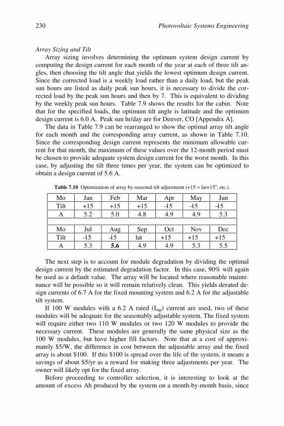
Photovoltaic Systems Engineering230
Array Sizing and TiltArray sizing involves determining the optimum system design current by
computing the design current for each month of the year at each of three tilt an-gles, then choosing the tilt angle that yields the lowest optimum design current.Since the corrected load is a weekly load rather than a daily load, but the peaksun hours are listed as daily peak sun hours, it is necessary to divide the cor-rected load by the peak sun hours and then by 7. This is equivalent to dividingby the weekly peak sun hours. Table 7.9 shows the results for the cabin. Notethat for the specified loads, the optimum tilt angle is latitude and the optimumdesign current is 6.0 A. Peak sun hr/day are for Denver, CO [Appendix A].
The data in Table 7.9 can be rearranged to show the optimal array tilt anglefor each month and the corresponding array current, as shown in Table 7.10.Since the corresponding design current represents the minimum allowable cur-rent for that month, the maximum of these values over the 12-month period mustbe chosen to provide adequate system design current for the worst month. In thiscase, by adjusting the tilt three times per year, the system can be optimized toobtain a design current of 5.6 A.
Table 7.10 Optimization of array by seasonal tilt adjustment (+15 = lat+15o, etc.).
Mo Jan Feb Mar Apr May JunTilt +15 +15 +15 –15 –15 –15A 5.2 5.0 4.8 4.9 4.9 5.3
Mo Jul Aug Sep Oct Nov DecTilt –15 –15 lat +15 +15 +15A 5.3 5.6 4.9 4.9 5.3 5.5
The next step is to account for module degradation by dividing the optimaldesign current by the estimated degradation factor. In this case, 90% will againbe used as a default value. The array will be located where reasonable mainte-nance will be possible so it will remain relatively clean. This yields derated de-sign currents of 6.7 A for the fixed mounting system and 6.2 A for the adjustabletilt system.
If 100 W modules with a 6.2 A rated (Imp) current are used, two of thesemodules will be adequate for the seasonably adjustable system. The fixed systemwill require either two 110 W modules or two 120 W modules to provide thenecessary current. These modules are generally the same physical size as the100 W modules, but have higher fill factors. Note that at a cost of approxi-mately $5/W, the difference in cost between the adjustable array and the fixedarray is about $100. If this $100 is spread over the life of the system, it means asavings of about $5/yr as a reward for making three adjustments per year. Theowner will likely opt for the fixed array.
Before proceeding to controller selection, it is interesting to look at theamount of excess Ah produced by the system on a month-by-month basis, since
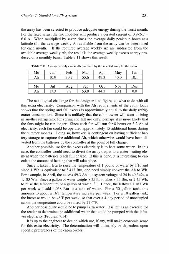
Chapter 7 Stand-Alone PV Systems 231
the array has been selected to produce adequate energy during the worst month.For the fixed array, the two modules will produce a derated current of 0.9 × 6.7 =6.0 A. When multiplied by seven times the average daily peak sun hours at alatitude tilt, the average weekly Ah available from the array can be determinedfor each month. If the required average weekly Ah are subtracted from theavailable average weekly Ah, the result is the average weekly excess energy pro-duced on a monthly basis. Table 7.11 shows this result.
Table 7.11 Average weekly excess Ah produced by the selected array for the cabin.
Mo Jan Feb Mar Apr May JunAh 10.9 30.7 55.6 49.3 40.0 10.1
Mo Jul Aug Sep Oct Nov DecAh 17.3 9.7 53.8 44.3 10.1 0.0
The next logical challenge for the designer is to figure out what to do with allthis extra electricity. Comparison with the Ah requirements of the cabin loadsshows that the spring and fall excess is approximately equal to the daily refrig-erator consumption. Since it is unlikely that the cabin owner will want to bringin another refrigerator for spring and fall use only, perhaps it is more likely thatthe fans might be run longer. Since each fan will run for 8 hours on 3.2 Ah ofelectricity, each fan could be operated approximately 15 additional hours duringthe summer months. Doing so, however, is contingent on having sufficient bat-tery storage to capture the additional Ah, which otherwise would have been di-verted from the batteries by the controller at the point of full charge.
Another possible use for the excess electricity is to heat some water. In thiscase, the controller would need to divert the array output to a water heating ele-ment when the batteries reach full charge. If this is done, it is interesting to cal-culate the amount of heating that will take place.
Since it takes 1 Btu to raise the temperature of 1 pound of water by 1oF, andsince 1 Wh is equivalent to 3.413 Btu, one need simply convert the Ah to Wh.For example, in April, the excess 49.3 Ah at a system voltage of 24 is 49.3 × 24 =1,183 Wh. Since a gallon of water weighs 8.35 lb, it takes 8.35 Btu, or 2.45 Wh,to raise the temperature of a gallon of water 1oF. Hence, the leftover 1,183 Whper week will add 4,038 Btu to a tank of water. For a 30 gallon tank, thisamounts to about a 16oF temperature increase per week. For a 10 gallon tank,the increase would be 48oF per week, so that over a 4-day period of unoccupiedcabin, the temperature could be raised by 27.6oF.
Another possibility would be to pump extra water. It is left as an exercise forthe reader to determine the additional water that could be pumped with the lefto-ver electricity (Problem 7.14).
It is up to the engineer to decide which use, if any, will make economic sensefor this extra electricity. The determination will ultimately be dependent uponspecific preferences of the cabin owner.
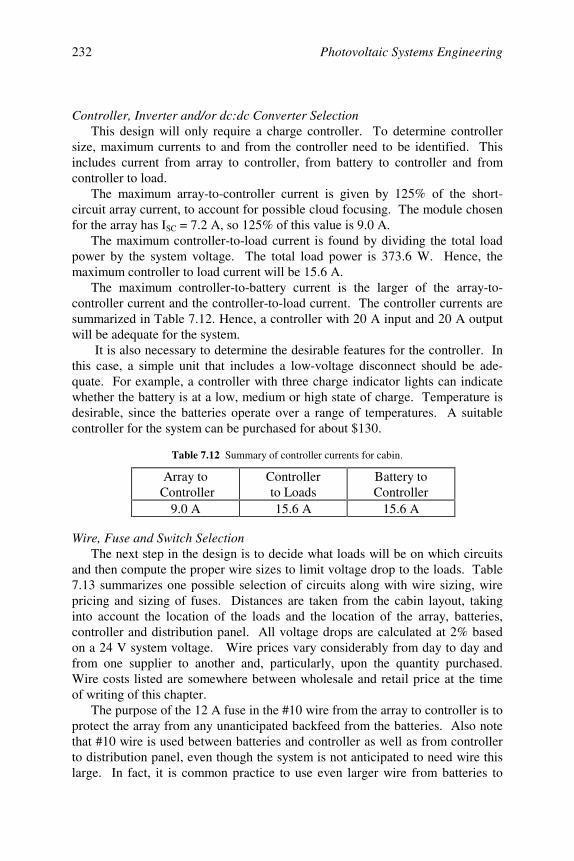
Photovoltaic Systems Engineering232
Controller, Inverter and/or dc:dc Converter SelectionThis design will only require a charge controller. To determine controller
size, maximum currents to and from the controller need to be identified. Thisincludes current from array to controller, from battery to controller and fromcontroller to load.
The maximum array-to-controller current is given by 125% of the short-circuit array current, to account for possible cloud focusing. The module chosenfor the array has ISC = 7.2 A, so 125% of this value is 9.0 A.
The maximum controller-to-load current is found by dividing the total loadpower by the system voltage. The total load power is 373.6 W. Hence, themaximum controller to load current will be 15.6 A.
The maximum controller-to-battery current is the larger of the array-to-controller current and the controller-to-load current. The controller currents aresummarized in Table 7.12. Hence, a controller with 20 A input and 20 A outputwill be adequate for the system.
It is also necessary to determine the desirable features for the controller. Inthis case, a simple unit that includes a low-voltage disconnect should be ade-quate. For example, a controller with three charge indicator lights can indicatewhether the battery is at a low, medium or high state of charge. Temperature isdesirable, since the batteries operate over a range of temperatures. A suitablecontroller for the system can be purchased for about $130.
Table 7.12 Summary of controller currents for cabin.
Array to Controller
Controllerto Loads
Battery toController
9.0 A 15.6 A 15.6 A
Wire, Fuse and Switch SelectionThe next step in the design is to decide what loads will be on which circuits
and then compute the proper wire sizes to limit voltage drop to the loads. Table7.13 summarizes one possible selection of circuits along with wire sizing, wirepricing and sizing of fuses. Distances are taken from the cabin layout, takinginto account the location of the loads and the location of the array, batteries,controller and distribution panel. All voltage drops are calculated at 2% basedon a 24 V system voltage. Wire prices vary considerably from day to day andfrom one supplier to another and, particularly, upon the quantity purchased.Wire costs listed are somewhere between wholesale and retail price at the timeof writing of this chapter.
The purpose of the 12 A fuse in the #10 wire from the array to controller is toprotect the array from any unanticipated backfeed from the batteries. Also notethat #10 wire is used between batteries and controller as well as from controllerto distribution panel, even though the system is not anticipated to need wire thislarge. In fact, it is common practice to use even larger wire from batteries to
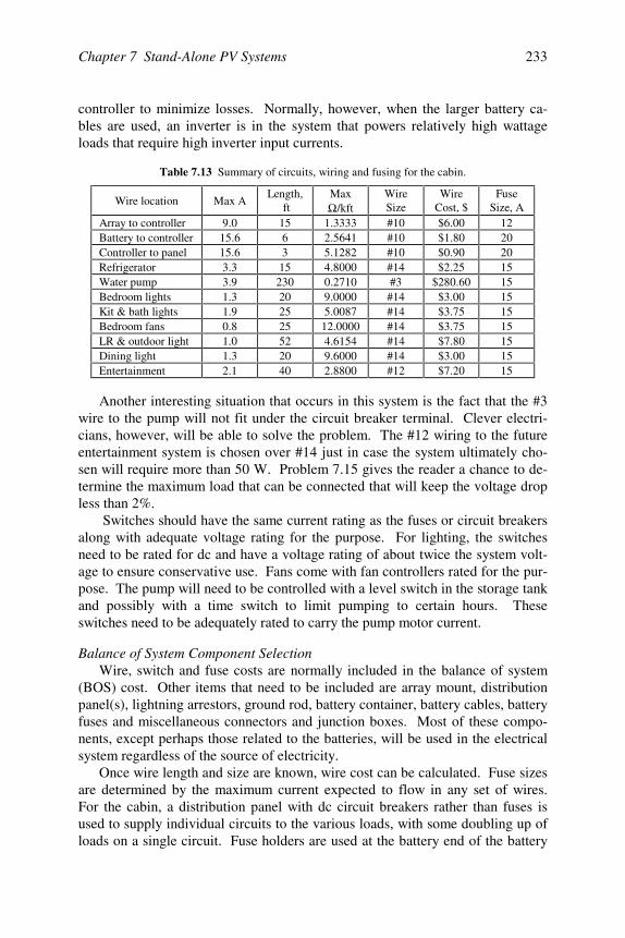
Chapter 7 Stand-Alone PV Systems 233
controller to minimize losses. Normally, however, when the larger battery ca-bles are used, an inverter is in the system that powers relatively high wattageloads that require high inverter input currents.
Table 7.13 Summary of circuits, wiring and fusing for the cabin.
Wire location Max ALength,
ftMaxΩ /kft
WireSize
WireCost, $
FuseSize, A
Array to controller 9.0 15 1.3333 #10 $6.00 12Battery to controller 15.6 6 2.5641 #10 $1.80 20Controller to panel 15.6 3 5.1282 #10 $0.90 20Refrigerator 3.3 15 4.8000 #14 $2.25 15Water pump 3.9 230 0.2710 #3 $280.60 15Bedroom lights 1.3 20 9.0000 #14 $3.00 15Kit & bath lights 1.9 25 5.0087 #14 $3.75 15Bedroom fans 0.8 25 12.0000 #14 $3.75 15LR & outdoor light 1.0 52 4.6154 #14 $7.80 15Dining light 1.3 20 9.6000 #14 $3.00 15Entertainment 2.1 40 2.8800 #12 $7.20 15
Another interesting situation that occurs in this system is the fact that the #3wire to the pump will not fit under the circuit breaker terminal. Clever electri-cians, however, will be able to solve the problem. The #12 wiring to the futureentertainment system is chosen over #14 just in case the system ultimately cho-sen will require more than 50 W. Problem 7.15 gives the reader a chance to de-termine the maximum load that can be connected that will keep the voltage dropless than 2%.
Switches should have the same current rating as the fuses or circuit breakersalong with adequate voltage rating for the purpose. For lighting, the switchesneed to be rated for dc and have a voltage rating of about twice the system volt-age to ensure conservative use. Fans come with fan controllers rated for the pur-pose. The pump will need to be controlled with a level switch in the storage tankand possibly with a time switch to limit pumping to certain hours. Theseswitches need to be adequately rated to carry the pump motor current.
Balance of System Component SelectionWire, switch and fuse costs are normally included in the balance of system
(BOS) cost. Other items that need to be included are array mount, distributionpanel(s), lightning arrestors, ground rod, battery container, battery cables, batteryfuses and miscellaneous connectors and junction boxes. Most of these compo-nents, except perhaps those related to the batteries, will be used in the electricalsystem regardless of the source of electricity.
Once wire length and size are known, wire cost can be calculated. Fuse sizesare determined by the maximum current expected to flow in any set of wires.For the cabin, a distribution panel with dc circuit breakers rather than fuses isused to supply individual circuits to the various loads, with some doubling up ofloads on a single circuit. Fuse holders are used at the battery end of the battery
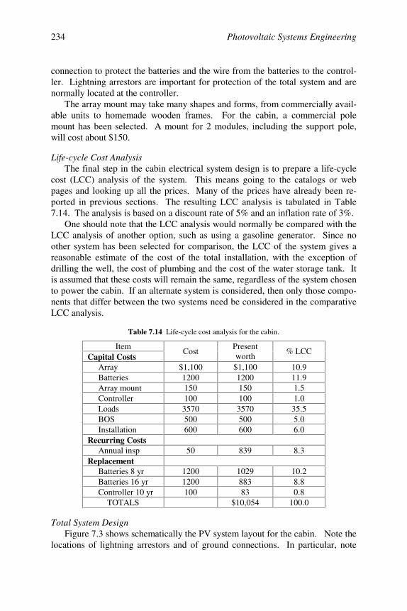
Photovoltaic Systems Engineering234
connection to protect the batteries and the wire from the batteries to the control-ler. Lightning arrestors are important for protection of the total system and arenormally located at the controller.
The array mount may take many shapes and forms, from commercially avail-able units to homemade wooden frames. For the cabin, a commercial polemount has been selected. A mount for 2 modules, including the support pole,will cost about $150.
Life-cycle Cost AnalysisThe final step in the cabin electrical system design is to prepare a life-cycle
cost (LCC) analysis of the system. This means going to the catalogs or webpages and looking up all the prices. Many of the prices have already been re-ported in previous sections. The resulting LCC analysis is tabulated in Table7.14. The analysis is based on a discount rate of 5% and an inflation rate of 3%.
One should note that the LCC analysis would normally be compared with theLCC analysis of another option, such as using a gasoline generator. Since noother system has been selected for comparison, the LCC of the system gives areasonable estimate of the cost of the total installation, with the exception ofdrilling the well, the cost of plumbing and the cost of the water storage tank. Itis assumed that these costs will remain the same, regardless of the system chosento power the cabin. If an alternate system is considered, then only those compo-nents that differ between the two systems need be considered in the comparativeLCC analysis.
Table 7.14 Life-cycle cost analysis for the cabin.
ItemCapital Costs
CostPresentworth
% LCC
Array $1,100 $1,100 10.9 Batteries 1200 1200 11.9 Array mount 150 150 1.5 Controller 100 100 1.0 Loads 3570 3570 35.5 BOS 500 500 5.0 Installation 600 600 6.0Recurring Costs Annual insp 50 839 8.3Replacement Batteries 8 yr 1200 1029 10.2 Batteries 16 yr 1200 883 8.8 Controller 10 yr 100 83 0.8
TOTALS $10,054 100.0
Total System DesignFigure 7.3 shows schematically the PV system layout for the cabin. Note the
locations of lightning arrestors and of ground connections. In particular, note
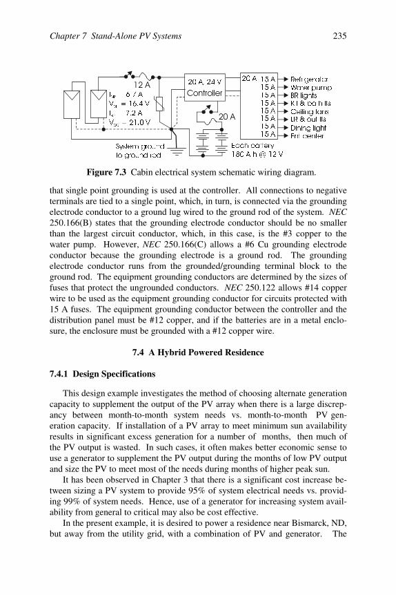
Chapter 7 Stand-Alone PV Systems 235
that single point grounding is used at the controller. All connections to negativeterminals are tied to a single point, which, in turn, is connected via the groundingelectrode conductor to a ground lug wired to the ground rod of the system. NEC250.166(B) states that the grounding electrode conductor should be no smallerthan the largest circuit conductor, which, in this case, is the #3 copper to thewater pump. However, NEC 250.166(C) allows a #6 Cu grounding electrodeconductor because the grounding electrode is a ground rod. The groundingelectrode conductor runs from the grounded/grounding terminal block to theground rod. The equipment grounding conductors are determined by the sizes offuses that protect the ungrounded conductors. NEC 250.122 allows #14 copperwire to be used as the equipment grounding conductor for circuits protected with15 A fuses. The equipment grounding conductor between the controller and thedistribution panel must be #12 copper, and if the batteries are in a metal enclo-sure, the enclosure must be grounded with a #12 copper wire.
7.4 A Hybrid Powered Residence
7.4.1 Design Specifications
This design example investigates the method of choosing alternate generationcapacity to supplement the output of the PV array when there is a large discrep-ancy between month-to-month system needs vs. month-to-month PV gen-eration capacity. If installation of a PV array to meet minimum sun availabilityresults in significant excess generation for a number of months, then much ofthe PV output is wasted. In such cases, it often makes better economic sense touse a generator to supplement the PV output during the months of low PV outputand size the PV to meet most of the needs during months of higher peak sun.
It has been observed in Chapter 3 that there is a significant cost increase be-tween sizing a PV system to provide 95% of system electrical needs vs. provid-ing 99% of system needs. Hence, use of a generator for increasing system avail-ability from general to critical may also be cost effective.
In the present example, it is desired to power a residence near Bismarck, ND,but away from the utility grid, with a combination of PV and generator. The
6\VWHPJURXQG
WRJURXQGURG
(DFKEDWWHU\
$K#9
$$$$$$$$
$
, $
9 9
, $
9 9
03
03
6&
2&
5HIULJHUDWRU:DWHUSXPS%5OLJKWV.LWEDWKOWV&HLOLQJIDQV/5RXWOWV
'LQLQJOLJKW(QWFHQWHU
Figure 7.3 Cabin electrical system schematic wiring diagram.
$9
Photovoltaic Systems Engineering236
residence will be occupied 7 days per week all year long. All loads will be 120V ac as in typical residences, except that energy efficiency has been taken intoaccount in the selection of the loads and the design of the dwelling. For exam-ple, a high efficiency refrigerator has been selected and all lighting will be fluo-rescent. The dwelling is designed with fans and is highly insulated with triple-pane glass in the windows. Much of the heating will be by passive solar, butpropane will be used for supplemental heating, solar water heating backup andcooking. Since propane will be on site, it will also be used for the generator.The goal of the design is to arrive at a combination of PV and propane generatorenergy production that will result in the lowest, or, at least acceptable, LCC.
7.4.2 Design Implementation
Since PV and generator output capability come in steps, this design processwill explore the LCC of several combinations of PV and generator. Up to thispoint little discussion of generator properties has taken place, so a part of thedesign discussion will deal with the selection of generators. The design processis somewhat modified from the previous examples, since the propane generatoralso needs to be sized and incorporated into the system. This means a morecomplicated system block diagram, resulting in a somewhat more challengingcontrol problem.
Since the generator is available for PV system backup, it may seem unneces-sary to incorporate batteries into the system. However, for generators to operateefficiently, they need to run at close to 90% of their output capacity. Operationof a generator at a small fraction of capacity will result in significant decrease inefficiency, as was noted in Chapter 3. Hence, batteries are used so the generatorcan charge them at a rate close to its capacity.
Since charging batteries too quickly tends to result in an inefficient chargingprocess, the generator/battery system should be sized so the generator will takeat least 5 hours to charge the batteries [2]. The battery selection criteria of Sec-tion 7.2 appear to present a more conservative requirement of at least 10 hours tofully charge the batteries. Actually, these criteria are not necessarily inconsis-tent, since the batteries will not normally be charged from full discharge to fullcharge. Normally the generator will charge the batteries from about 20% toabout 70%. Charging the batteries from 20 to 70% in 5 hours requires a charg-ing rate of C/10.
The bottom line, then, for batteries, is to provide a few days of storage so thecharging rate will not be excessive. More storage will normally result in some-what lower use of the generator, since the generator will not necessarily need toback up the PV array in the event of cloudy weather for a few days. Longerstorage times may be desirable in areas where summers have periods of sunnydays followed by periods of cloudy days. In general, fewer batteries will be usedin a hybrid system since the propane generator will supplement the sun. Choiceof the number of days of autonomy for the system, however, becomes more de-
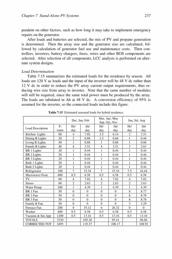
Chapter 7 Stand-Alone PV Systems 237
pendent on other factors, such as how long it may take to implement emergencyrepairs on the generator.
After loads and batteries are selected, the mix of PV and propane generationis determined. Then the array size and the generator size are calculated, fol-lowed by calculation of generator fuel use and maintenance costs. Then con-trollers, inverters, battery chargers, fuses, wires and other BOS components areselected. After selection of all components, LCC analysis is performed on alter-nate system designs.
Load DeterminationTable 7.15 summarizes the estimated loads for the residence by season. All
loads are 120 V ac loads and the input of the inverter will be 48 V dc rather than12 V dc in order to reduce the PV array current output requirements, thus re-ducing wire size from array to inverter. Note that the same number of moduleswill still be required, since the same total power must be produced by the array.The loads are tabulated in Ah at 48 V dc. A conversion efficiency of 95% isassumed for the inverter, so the connected loads include this figure.
Table 7.15 Estimated seasonal loads for hybrid residence.
Dec, Jan, FebMar, Apr, MaySep, Oct, Nov
Jun, Jul, Aug
Load DescriptionP,
wattsHr/day
Ah/day
Hr/day
Ah/day
Hr/day
Ah/day
Kitchen Lights 80 4 7.02 3.5 6.14 2 3.51Dining R Lights 20 2 0.88 1.5 0.66 1 0.44Living R Lights 40 1 0.88 1 0.88 1 0.88Family R Lights 40 4 3.51 4 3.51 3 2.63BR 1 Lights 20 1 0.44 1 0.44 1 0.44BR 2 Lights 20 1 0.44 1 0.44 1 0.44BR 3 Lights 20 1 0.44 1 0.44 1 0.44Bath 1 Lights 20 1 0.44 1 0.44 1 0.44Bath 2 Lights 20 1 0.44 1 0.44 1 0.44Refrigerator 100 7 15.34 7 15.34 7.5 16.44Microwave Oven 600 0.5 6.58 0.5 6.58 0.5 6.58TV 80 4 7.02 4 7.02 4 7.02Stereo 60 2 2.63 2 2.63 2 2.63Water Pump 200 1 4.39 1 4.39 1 4.39BR 1 Fan 50 0 0 0 0 8 8.77BR 2 Fan 50 0 0 0 0 8 8.78BR 3 Fan 50 0 0 0 0 8 8.78Family R Fan 50 0 0 0 0 3 3.29Furnace Fan 200 8 35.12 6 26.32 0 0Washer 600 0.5 6.58 0.5 6.58 0.5 6.58Vacuum & Sm App 1200 0.5 13.16 0.5 13.16 0.5 13.16TOTALS 3320 105.28 95.41 96.06CORRECTED TOT 3495 119.37 108.17 108.92
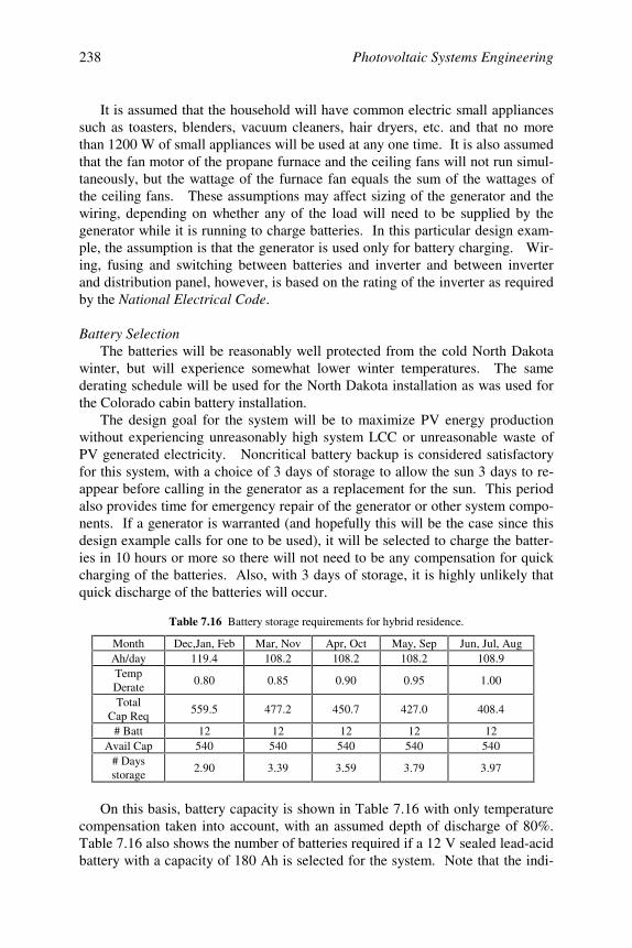
Photovoltaic Systems Engineering238
It is assumed that the household will have common electric small appliancessuch as toasters, blenders, vacuum cleaners, hair dryers, etc. and that no morethan 1200 W of small appliances will be used at any one time. It is also assumedthat the fan motor of the propane furnace and the ceiling fans will not run simul-taneously, but the wattage of the furnace fan equals the sum of the wattages ofthe ceiling fans. These assumptions may affect sizing of the generator and thewiring, depending on whether any of the load will need to be supplied by thegenerator while it is running to charge batteries. In this particular design exam-ple, the assumption is that the generator is used only for battery charging. Wir-ing, fusing and switching between batteries and inverter and between inverterand distribution panel, however, is based on the rating of the inverter as requiredby the National Electrical Code.
Battery SelectionThe batteries will be reasonably well protected from the cold North Dakota
winter, but will experience somewhat lower winter temperatures. The samederating schedule will be used for the North Dakota installation as was used forthe Colorado cabin battery installation.
The design goal for the system will be to maximize PV energy productionwithout experiencing unreasonably high system LCC or unreasonable waste ofPV generated electricity. Noncritical battery backup is considered satisfactoryfor this system, with a choice of 3 days of storage to allow the sun 3 days to re-appear before calling in the generator as a replacement for the sun. This periodalso provides time for emergency repair of the generator or other system compo-nents. If a generator is warranted (and hopefully this will be the case since thisdesign example calls for one to be used), it will be selected to charge the batter-ies in 10 hours or more so there will not need to be any compensation for quickcharging of the batteries. Also, with 3 days of storage, it is highly unlikely thatquick discharge of the batteries will occur.
Table 7.16 Battery storage requirements for hybrid residence.
Month Dec,Jan, Feb Mar, Nov Apr, Oct May, Sep Jun, Jul, AugAh/day 119.4 108.2 108.2 108.2 108.9TempDerate
0.80 0.85 0.90 0.95 1.00
TotalCap Req
559.5 477.2 450.7 427.0 408.4
# Batt 12 12 12 12 12Avail Cap 540 540 540 540 540
# Daysstorage
2.90 3.39 3.59 3.79 3.97
On this basis, battery capacity is shown in Table 7.16 with only temperaturecompensation taken into account, with an assumed depth of discharge of 80%.Table 7.16 also shows the number of batteries required if a 12 V sealed lead-acidbattery with a capacity of 180 Ah is selected for the system. Note that the indi-
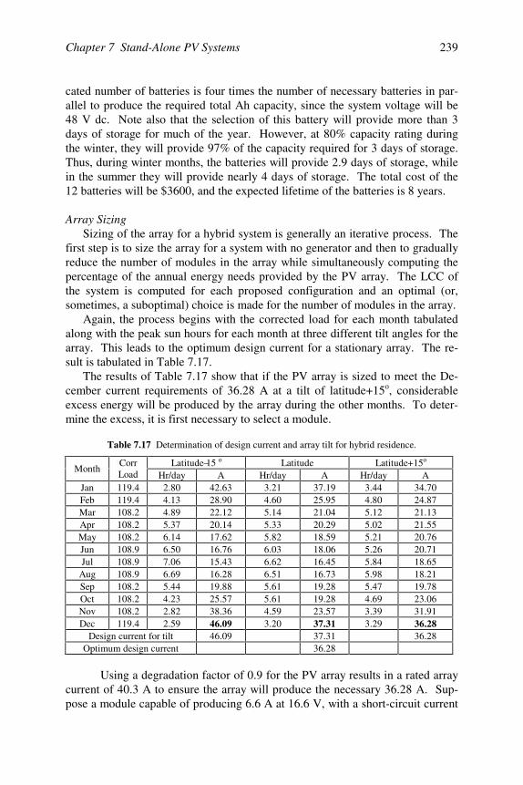
Chapter 7 Stand-Alone PV Systems 239
cated number of batteries is four times the number of necessary batteries in par-allel to produce the required total Ah capacity, since the system voltage will be48 V dc. Note also that the selection of this battery will provide more than 3days of storage for much of the year. However, at 80% capacity rating duringthe winter, they will provide 97% of the capacity required for 3 days of storage.Thus, during winter months, the batteries will provide 2.9 days of storage, whilein the summer they will provide nearly 4 days of storage. The total cost of the12 batteries will be $3600, and the expected lifetime of the batteries is 8 years.
Array SizingSizing of the array for a hybrid system is generally an iterative process. The
first step is to size the array for a system with no generator and then to graduallyreduce the number of modules in the array while simultaneously computing thepercentage of the annual energy needs provided by the PV array. The LCC ofthe system is computed for each proposed configuration and an optimal (or,sometimes, a suboptimal) choice is made for the number of modules in the array.
Again, the process begins with the corrected load for each month tabulatedalong with the peak sun hours for each month at three different tilt angles for thearray. This leads to the optimum design current for a stationary array. The re-sult is tabulated in Table 7.17.
The results of Table 7.17 show that if the PV array is sized to meet the De-cember current requirements of 36.28 A at a tilt of latitude+15o, considerableexcess energy will be produced by the array during the other months. To deter-mine the excess, it is first necessary to select a module.
Table 7.17 Determination of design current and array tilt for hybrid residence.
Latitude–15 o Latitude Latitude+15o
MonthCorrLoad Hr/day A Hr/day A Hr/day A
Jan 119.4 2.80 42.63 3.21 37.19 3.44 34.70Feb 119.4 4.13 28.90 4.60 25.95 4.80 24.87Mar 108.2 4.89 22.12 5.14 21.04 5.12 21.13Apr 108.2 5.37 20.14 5.33 20.29 5.02 21.55May 108.2 6.14 17.62 5.82 18.59 5.21 20.76Jun 108.9 6.50 16.76 6.03 18.06 5.26 20.71Jul 108.9 7.06 15.43 6.62 16.45 5.84 18.65
Aug 108.9 6.69 16.28 6.51 16.73 5.98 18.21Sep 108.2 5.44 19.88 5.61 19.28 5.47 19.78Oct 108.2 4.23 25.57 5.61 19.28 4.69 23.06Nov 108.2 2.82 38.36 4.59 23.57 3.39 31.91Dec 119.4 2.59 46.09 3.20 37.31 3.29 36.28
Design current for tilt 46.09 37.31 36.28Optimum design current 36.28
Using a degradation factor of 0.9 for the PV array results in a rated arraycurrent of 40.3 A to ensure the array will produce the necessary 36.28 A. Sup-pose a module capable of producing 6.6 A at 16.6 V, with a short-circuit current
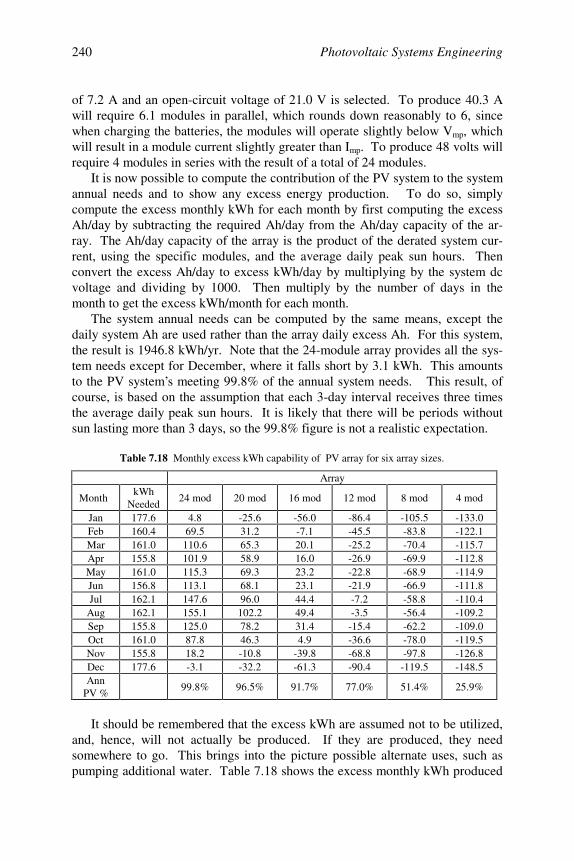
Photovoltaic Systems Engineering240
of 7.2 A and an open-circuit voltage of 21.0 V is selected. To produce 40.3 Awill require 6.1 modules in parallel, which rounds down reasonably to 6, sincewhen charging the batteries, the modules will operate slightly below Vmp, whichwill result in a module current slightly greater than Imp. To produce 48 volts willrequire 4 modules in series with the result of a total of 24 modules.
It is now possible to compute the contribution of the PV system to the systemannual needs and to show any excess energy production. To do so, simplycompute the excess monthly kWh for each month by first computing the excessAh/day by subtracting the required Ah/day from the Ah/day capacity of the ar-ray. The Ah/day capacity of the array is the product of the derated system cur-rent, using the specific modules, and the average daily peak sun hours. Thenconvert the excess Ah/day to excess kWh/day by multiplying by the system dcvoltage and dividing by 1000. Then multiply by the number of days in themonth to get the excess kWh/month for each month.
The system annual needs can be computed by the same means, except thedaily system Ah are used rather than the array daily excess Ah. For this system,the result is 1946.8 kWh/yr. Note that the 24-module array provides all the sys-tem needs except for December, where it falls short by 3.1 kWh. This amountsto the PV system’s meeting 99.8% of the annual system needs. This result, ofcourse, is based on the assumption that each 3-day interval receives three timesthe average daily peak sun hours. It is likely that there will be periods withoutsun lasting more than 3 days, so the 99.8% figure is not a realistic expectation.
Table 7.18 Monthly excess kWh capability of PV array for six array sizes.
Array
MonthkWh
Needed24 mod 20 mod 16 mod 12 mod 8 mod 4 mod
Jan 177.6 4.8 -25.6 -56.0 -86.4 -105.5 -133.0Feb 160.4 69.5 31.2 -7.1 -45.5 -83.8 -122.1Mar 161.0 110.6 65.3 20.1 -25.2 -70.4 -115.7Apr 155.8 101.9 58.9 16.0 -26.9 -69.9 -112.8May 161.0 115.3 69.3 23.2 -22.8 -68.9 -114.9Jun 156.8 113.1 68.1 23.1 -21.9 -66.9 -111.8Jul 162.1 147.6 96.0 44.4 -7.2 -58.8 -110.4
Aug 162.1 155.1 102.2 49.4 -3.5 -56.4 -109.2Sep 155.8 125.0 78.2 31.4 -15.4 -62.2 -109.0Oct 161.0 87.8 46.3 4.9 -36.6 -78.0 -119.5Nov 155.8 18.2 -10.8 -39.8 -68.8 -97.8 -126.8Dec 177.6 -3.1 -32.2 -61.3 -90.4 -119.5 -148.5Ann
PV %99.8% 96.5% 91.7% 77.0% 51.4% 25.9%
It should be remembered that the excess kWh are assumed not to be utilized,and, hence, will not actually be produced. If they are produced, they needsomewhere to go. This brings into the picture possible alternate uses, such aspumping additional water. Table 7.18 shows the excess monthly kWh produced
Chapter 7 Stand-Alone PV Systems 241
by the PV array for the 24-module array as well as for arrays of 20, 16, 12, 8 and4 modules. The table also shows the percentage of annual system kWh require-ments supplied by these arrays. Normally, when the PV system provides lessthan 95% of the system needs, an alternate source of electricity is incorporatedinto the system. Hence, in this case, the 20-module system should provide goodsystem performance year around without any backup, provided that the dwellingoccupants reduce energy consumption in the winter.
Generator SizingThe generator should be sized to charge the batteries at approximately C/10
as indicated previously. At this rate of charging, the generator should be oper-ating at approximately 80 to 90% of its rated output in order to ensure maximumgenerator efficiency. Hence, it is first necessary to determine what C/10 meansfor this system.
The first question when analyzing Table 7.16, is Which capacity should beused in determining C/10? With temperature derating applied, the batteries havea capacity of 432 Ah in the winter and 540 Ah in the summer. Since most gen-erator operation will be in the winter, as indicated by Table 7.18, the winter ca-pacity is the appropriate choice. Hence, 43.2 A for 10 hours will produce 432Ah of charge.
The generator will be rated in watts. Thus, it is necessary to determine thepower, rather than the Ah requirements of the batteries. This is obtained by in-corporating the battery-charging voltage. For a C/10 charging rate, the batterycharger output power will thus be the product of the charging voltage and thecharging current, or 48 × 1.2 × 43.2 = 2488 W, since the charging voltage is gener-ally about 120% of the nominal battery voltage. If the electrical conversion effi-ciency of the battery charger is 90%, this would require an input power of2488 ÷ 0.9 = 2764 W to provide 43.2 A of charging current. Since the generatoris to be used only for battery charging, a 2500 W generator would be a goodchoice, since it will run close to its rated output and will charge at a rate slightlyless than C/10.
If it is desired to have the generator run part of the load while charging thebatteries, or to charge at a faster rate, it would be reasonable to select the nextlarger size generator. However, the 2500 W unit operating at 2250 W willcharge the batteries from 20% to 70% in 6.14 hours. This is normally an accept-able charge rate, especially since it will take 5/8 of 2.9 days to use this amount ofcharge for this particular system. Charging the batteries to only 70% allows forthe PV array to top off the charge if it can. If not, and the batteries discharge to20% again, the generator comes on again.
Generator Operating CostThe more the generator runs, the more it will cost to operate. Generator op-
erating cost consists of fuel cost, oil changes, tune-ups and rebuilding. To de-
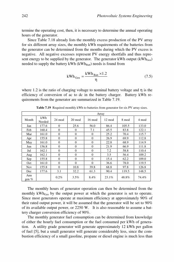
Photovoltaic Systems Engineering242
termine the operating cost, then, it is necessary to determine the annual operatinghours of the generator.
Since Table 7.18 already lists the monthly excess production of the PV arrayfor six different array sizes, the monthly kWh requirements of the batteries fromthe generator can be determined from the months during which the PV excess isnegative. All negative excesses represent PV energy shortfalls and thus repre-sent energy to be supplied by the generator. The generator kWh output (kWhGen)needed to supply the battery kWh (kWhBatt) needs is found from
η×
=2.1kWh
kWh BattGen (7.5)
where 1.2 is the ratio of charging voltage to nominal battery voltage and η is theefficiency of conversion of ac to dc in the battery charger. Battery kWh re-quirements from the generator are summarized in Table 7.19.
Table 7.19 Required monthly kWh to batteries from generator for six PV array sizes.
Array
MonthkWh
Needed24 mod 20 mod 16 mod 12 mod 8 mod 4 mod
Jan 177.6 0 25.6 56.0 86.4 105.5 133.0Feb 160.4 0 0 7.1 45.5 83.8 122.1Mar 161.0 0 0 0 25.2 70.4 115.7Apr 155.8 0 0 0 26.9 69.9 112.8May 161.0 0 0 0 22.8 68.9 114.9Jun 156.8 0 0 0 21.9 66.9 111.8Jul 162.1 0 0 0 7.2 58.8 110.4
Aug 162.1 0 0 0 3.5 56.4 109.2Sep 155.8 0 0 0 15.4 62.2 109.0Oct 161.0 0 0 0 36.6 78.0 119.5Nov 155.8 0 10.8 39.8 68.8 97.8 126.8Dec 177.6 3.1 32.2 61.3 90.4 119.5 148.5Ann
gen %0.2% 3.5% 8.4% 23.1% 48.8% 74.4%
The monthly hours of generator operation can then be determined from themonthly kWhGen by the output power at which the generator is set to operate.Since most generators operate at maximum efficiency at approximately 90% oftheir rated output power, it will be assumed that the generator will be set to 90%of its available output power, or 2250 W. It is also reasonable to assume a bat-tery charger conversion efficiency of 90%.
The monthly generator fuel consumption can be determined from knowledgeof either the hourly fuel consumption or the fuel consumed per kWh of genera-tion. A utility grade generator will generate approximately 12 kWh per gallonof fuel [5], but a small generator will generate considerably less, since the com-bustion efficiency of a small gasoline, propane or diesel engine is much less than
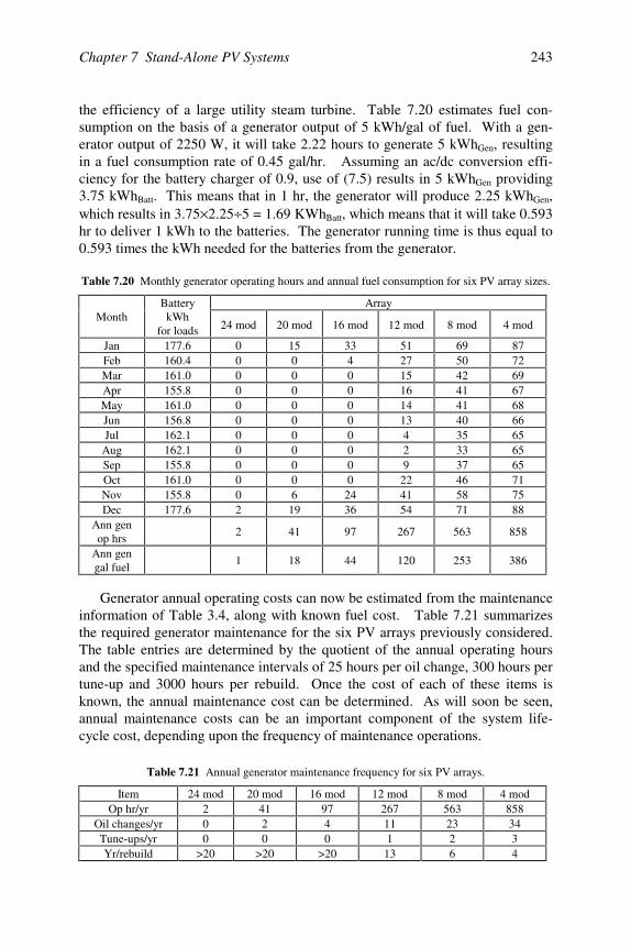
Chapter 7 Stand-Alone PV Systems 243
the efficiency of a large utility steam turbine. Table 7.20 estimates fuel con-sumption on the basis of a generator output of 5 kWh/gal of fuel. With a gen-erator output of 2250 W, it will take 2.22 hours to generate 5 kWhGen, resultingin a fuel consumption rate of 0.45 gal/hr. Assuming an ac/dc conversion effi-ciency for the battery charger of 0.9, use of (7.5) results in 5 kWhGen providing3.75 kWhBatt. This means that in 1 hr, the generator will produce 2.25 kWhGen,which results in 3.75 × 2.25 ÷ 5 = 1.69 KWhBatt, which means that it will take 0.593hr to deliver 1 kWh to the batteries. The generator running time is thus equal to0.593 times the kWh needed for the batteries from the generator.
Table 7.20 Monthly generator operating hours and annual fuel consumption for six PV array sizes.
ArrayMonth
BatterykWh
for loads 24 mod 20 mod 16 mod 12 mod 8 mod 4 mod
Jan 177.6 0 15 33 51 69 87Feb 160.4 0 0 4 27 50 72Mar 161.0 0 0 0 15 42 69Apr 155.8 0 0 0 16 41 67May 161.0 0 0 0 14 41 68Jun 156.8 0 0 0 13 40 66Jul 162.1 0 0 0 4 35 65
Aug 162.1 0 0 0 2 33 65Sep 155.8 0 0 0 9 37 65Oct 161.0 0 0 0 22 46 71Nov 155.8 0 6 24 41 58 75Dec 177.6 2 19 36 54 71 88
Ann genop hrs
2 41 97 267 563 858
Ann gengal fuel
1 18 44 120 253 386
Generator annual operating costs can now be estimated from the maintenanceinformation of Table 3.4, along with known fuel cost. Table 7.21 summarizesthe required generator maintenance for the six PV arrays previously considered.The table entries are determined by the quotient of the annual operating hoursand the specified maintenance intervals of 25 hours per oil change, 300 hours pertune-up and 3000 hours per rebuild. Once the cost of each of these items isknown, the annual maintenance cost can be determined. As will soon be seen,annual maintenance costs can be an important component of the system life-cycle cost, depending upon the frequency of maintenance operations.
Table 7.21 Annual generator maintenance frequency for six PV arrays.
Item 24 mod 20 mod 16 mod 12 mod 8 mod 4 modOp hr/yr 2 41 97 267 563 858
Oil changes/yr 0 2 4 11 23 34Tune-ups/yr 0 0 0 1 2 3Yr/rebuild >20 >20 >20 13 6 4
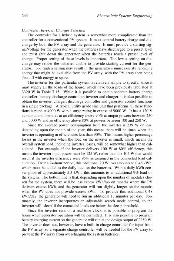
Photovoltaic Systems Engineering244
Controller, Inverter, Charger SelectionThe controller for a hybrid system is somewhat more complicated than the
controller for a conventional PV system. It must control battery charge and dis-charge by both the PV array and the generator. It must provide a starting sig-nal/voltage for the generator when the batteries have discharged to a preset leveland must shut down the generator when the batteries reach a preset level ofcharge. Proper setting of these levels is important. Too low a setting on dis-charge may render the batteries unable to provide starting current for the gen-erator. Too high a setting may result in the generator’s unnecessarily replacingenergy that might be available from the PV array, with the PV array then beingshut off with energy to spare.
The inverter for this particular system is relatively simple to specify, since itmust supply all the loads of the house, which have been previously tabulated at3320 W in Table 7.15. While it is possible to obtain separate battery chargecontroller, battery discharge controller, inverter and charger, it is also possible toobtain the inverter, charger, discharge controller and generator control functionsin a single package. A typical utility grade sine unit that performs all these func-tions is rated at 4000 W with a surge rating in excess of 9000 W. It has a 120 Vac output and operates at an efficiency above 90% at output powers between 250and 3000 W and an efficiency above 80% at powers between 100 and 250 W.
Since the average power consumption from the inverter is 239 W or less,depending upon the month of the year, this means there will be times when theinverter is operating at efficiencies less than 90%. This means higher percentagelosses in the inverter when the load on the inverter is small, which means theoverall system load, including inverter losses, will be somewhat higher than cal-culated. For example, if the inverter delivers 100 W at 80% efficiency, thismeans the inverter input power must be 125 W, rather than the 105 W that wouldresult if the inverter efficiency were 95% as assumed in the connected load cal-culation. Over a 24-hour period, this additional 20 W loss amounts to 0.48 kWh,which must be added to the daily load on the batteries. With a daily kWh con-sumption of approximately 5.3 kWh, this amounts to an additional 9% load onthe system. The bottom line is that, depending upon the number of modules cho-sen for the system, there will be less excess kWh/mo on months where the PVdelivers excess kWh, and the generator will run slightly longer on the monthswhen the PV does not provide excess kWh. To provide this additional 0.48kWh/day, the generator will need to run an additional 17 minutes per day. For-tunately, the inverter incorporates an adjustable search mode control, so theinverter will “sleep” if the connected loads are below the slee p threshold.
Since the inverter runs on a real-time clock, it is possible to program thehours when generator operation will be permitted. It is also possible to programbattery charging current so the generator will run at the design output of 2250 W.The inverter does not, however, have a built-in charge controller for input fromthe PV array, so a separate charge controller will be needed for the PV array toprevent the PV array from overcharging the system batteries.
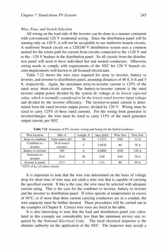
Chapter 7 Stand-Alone PV Systems 245
Wire, Fuse, and Switch SelectionAll wiring on the load side of the inverter can be done in a manner consistent
with conventional 120 V residential wiring. Since the distribution panel will berunning only on 120 V, it will not be acceptable to use multiwire branch circuits.A multiwire branch circuit on a 120/240 V distribution system uses a commonneutral for the return path for current from circuits connected to the +120 V andto the −120 V busbars in the distribution panel. So all circuits from the distribu-tion panel will need to have individual hot and neutral conductors. Otherwisewiring needs to comply with requirements of the NEC for 120 V branch cir-cuits—requirements well known to all licensed electricians.
Table 7.22 shows the wire sizes required for array to inverter, battery toinverter, and inverter to distribution panel, assuming distances of 40 ft, 6 ft and 5ft, respectively. Again, the maximum array-to-inverter current is 125% of therated array short-circuit current. The battery-to-inverter current is the ratedinverter output power divided by the system dc voltage at its lowest expectedvalue, which is normally considered to be the lowest rated inverter input voltageand divided by the inverter efficiency. The inverter-to-panel current is deter-mined from the rated inverter output power, divided by 120 V. Wiring must besized to carry 125% of these rated currents. For the wiring from generator toinverter/charger, the wire must be sized to carry 115% of the rated generatoroutput current, per NEC.
Table 7.22 Summary of PV circuits, wiring and fusing for the hybrid residence.
Wire location Max A Length, ft Max Ω /kft Wire Size Fuse SizeArray to combiner 9 per source ckt* 40 1.3333 #10 12 A
Combiner toinverter
54 (6 sourcecircuits)
3 2.9630 #6 70 A
Battery to inverter 100 6 0.8000 #2/0 150 AGenerator to
inverter20.8 20 2.88 #10 30 A
Inverter to panel 33.3 5 7.21 #8 50 A*125% of ISC of source circuit.
It is important to note that the wire size determined on the basis of voltagedrop for short runs of wire may not yield a wire size that is capable of carryingthe specified current. If this is the case, the wire must be selected with adequatecurrent rating. This is the case for the combiner to inverter, battery to inverterand the inverter to distribution panel. If wires operate at temperatures in excessof 30°C, or if more than three current carrying conductors are in a conduit, thewire ampacity must be further derated. These procedures will be carried out inthe examples of Chapter 8. Correct wire sizes are listed in the table.
It is also interesting to note that the load and distribution panel size calcu-lated in this example are considerably less than the minimum service size re-quired by the National Electrical Code. The local electrical inspector is theultimate authority on the application of the NEC. The inspector may accept a
Photovoltaic Systems Engineering246
design certified by a registered professional electrical engineer, or the inspectormay insist on wiring of adequate size to meet minimum NEC requirements. Theconcern would be that the dwelling may one day be powered by abundant utilitypower if the grid should be extended to the location of the dwelling.
Balance-of-System Component SelectionThe BOS components will include a battery storage container, an array
mount, surge protection and provisions for proper grounding of the system. Ofcourse, the wiring from the distribution panel is also a part of the balance of thesystem, but its cost will not change as the mix of PV vs. propane generation isvaried. The cost of the array mount and the cost of wire from array to combinerbox are the only items in the BOS that will vary with the number of modules.
Life-cycle Cost AnalysisIn order to determine the optimum mix of PV and generator-produced kWh,
it is necessary to compute the LCC of several mixes and hope to obtain a curvethat will show a minimum cost for a particular mix. However, if the system costeither increases or decreases monotonically, then no such minimum will exist.The LCC computation must take into account the costs of all system componentsthat will vary as the generation mix is changed. This includes array cost, arraymount cost, generator operating and maintenance costs and controller/invertercost. In the ideal case, a price should be affixed to the relative environmentalcosts of each type of generation. While this will not be done for this example,environmental costs will be discussed in Chapter 9. In this chapter, it will sim-ply be assumed that the less the generator runs, the less noise and air pollutionwill be created.
Table 7.23 shows the LCC analysis for a 24-module array with no generatorand a 12-module array with a generator that must supply 23.1% of the annualenergy needs. Reasonable assumptions are made for fuel cost and maintenancecost for the generator. It is assumed that propane costs $1.50 per gallon, an oilchange will cost $5, a tune-up will cost $50 and a rebuild will cost $375. Arraymount costs are based on the cost of typical commercial array mounts. It is as-sumed that the inverter for the hybrid system will be the same as the inverter forthe nonhybrid system to allow for addition of a generator at a later date if de-sired. The installation cost is assumed to be $1/W for the PV system plus 20%of the cost of the generator. The LCC is based on a discount rate of 5% and aninflation rate of 3%.
Figure 7.4a is a plot of LCC vs. the number of modules in the system, andFigure 7.4b is a plot of the LCC vs. the percent of annual kWh provided by thePV array. It is now up to the system owner to decide whether to spend the ad-ditional $1808 for the convenience of the 100% PV system or to choose a com-promise figure. Perhaps the biggest surprise is the LCC of the generator-onlysystem. It must be remembered that the system also includes an inverter andbatteries so the generator need not run continuously and can run at its most effi-
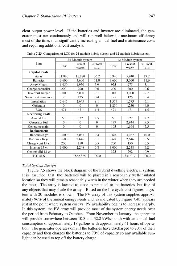
Chapter 7 Stand-Alone PV Systems 247
cient output power level. If the batteries and inverter are eliminated, the gen-erator must run continuously and will run well below its maximum efficiencymost of the time, thus significantly increasing annual fuel and maintenance costsand requiring additional cost analysis.
Table 7.23 Comparison of LCC for 24-module hybrid system and 12-module hybrid system.
24-Module system 12-Module systemItem
CostPresentWorth
% TotalLCC
CostPresentWorth
% TotalLCC
Capital CostsArray 11,880 11,880 36.2 5,940 5,940 19.2
Batteries 3,600 3,600 11.0 3,600 3,600 11.6Array Mount 1,950 1,950 5.9 975 975 3.1
Charge controller 200 200 0.6 200 200 0.6Inverter/Charger 3,000 3,000 9.1 3,000 3,000 9.7
Source ckt combiner 125 125 0.4 125 125 0.4Installation 2,645 2,645 8.1 1,573 1,573 5.1Generator 0 0 0 1,250 1,250 4.0
BOS 471 471 1.4 471 471 1.5Recurring Costs
Annual Insp 50 822 2.5 50 822 2.7Generator fuel 0 0 0 179 2,944 9.5
Generator maint 0 0 0 103 1,694 5.5ReplacementBatteries 8 yr 3,600 3,087 9.4 3,600 3,087 10.0
Batteries 16 yr 3,600 2,646 8.1 3,600 2,646 8.5Charge cont 15 yr 200 150 0.5 200 150 0.5
Inverter 15 yr 3,000 2,248 6.8 3,000 2,248 7.2Gen rebuild 13 yr 375 292 0.9
TOTALS $32,825 100.0 $31,017 100.0
Total System DesignFigure 7.5 shows the block diagram of the hybrid dwelling electrical system.
It is assumed that the batteries will be placed in a reasonably well-insulatedlocation so they will remain reasonably warm in the winter when they are neededthe most. The array is located as close as practical to the batteries, but free ofany objects that may shade the array. Based on the life-cycle cost figures, a sys-tem with 20 modules is shown. The PV array of this system supplies approxi-mately 96% of the annual energy needs and, as indicated by Figure 7.4b, appearsjust at the point where system cost vs. PV availability begins to increase sharply.In this system, the PV array will provide most of the system energy needs overthe period from February to October. From November to January, the generatorwill provide somewhere between 10.8 and 32.2 kWh/month with an annual fuelconsumption of approximately 18 gallons with approximately 41 hours of opera-tion. The generator operates only if the batteries have discharged to 20% of theircapacity and then charges the batteries to 70% of capacity so any available sun-light can be used to top off the battery charge.
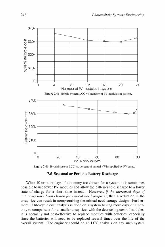
Photovoltaic Systems Engineering248
7.5 Seasonal or Periodic Battery Discharge
When 10 or more days of autonomy are chosen for a system, it is sometimespossible to use fewer PV modules and allow the batteries to discharge to a lowerstate of charge for a short time instead. However, if the increased days ofautonomy have been chosen for critical need purposes, then a reduction in thearray size can result in compromising the critical need storage design. Further-more, if life-cycle cost analysis is done on a system having more days of auton-omy to compensate for a smaller array size, with the decreasing cost of modules,it is normally not cost-effective to replace modules with batteries, especiallysince the batteries will need to be replaced several times over the life of theoverall system. The engineer should do an LCC analysis on any such system
% &'(!
Figure 7.4b Hybrid system LCC vs. percent of annual kWh supplied by PV array.
)
% * +&
,(
,(
,-(
,(
Figure 7.4a Hybrid system LCC vs. number of PV modules in system.
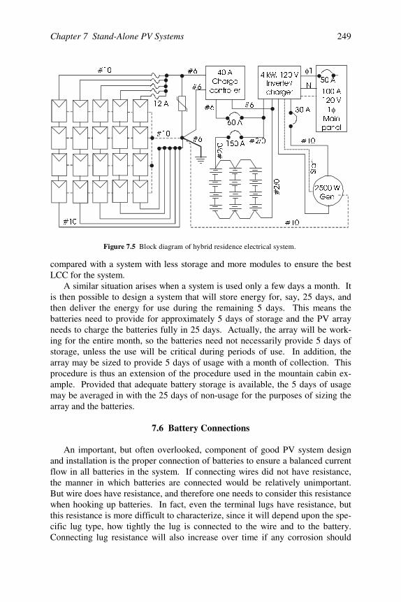
Chapter 7 Stand-Alone PV Systems 249
compared with a system with less storage and more modules to ensure the bestLCC for the system.
A similar situation arises when a system is used only a few days a month. Itis then possible to design a system that will store energy for, say, 25 days, andthen deliver the energy for use during the remaining 5 days. This means thebatteries need to provide for approximately 5 days of storage and the PV arrayneeds to charge the batteries fully in 25 days. Actually, the array will be work-ing for the entire month, so the batteries need not necessarily provide 5 days ofstorage, unless the use will be critical during periods of use. In addition, thearray may be sized to provide 5 days of usage with a month of collection. Thisprocedure is thus an extension of the procedure used in the mountain cabin ex-ample. Provided that adequate battery storage is available, the 5 days of usagemay be averaged in with the 25 days of non-usage for the purposes of sizing thearray and the batteries.
7.6 Battery Connections
An important, but often overlooked, component of good PV system designand installation is the proper connection of batteries to ensure a balanced currentflow in all batteries in the system. If connecting wires did not have resistance,the manner in which batteries are connected would be relatively unimportant.But wire does have resistance, and therefore one needs to consider this resistancewhen hooking up batteries. In fact, even the terminal lugs have resistance, butthis resistance is more difficult to characterize, since it will depend upon the spe-cific lug type, how tightly the lug is connected to the wire and to the battery.Connecting lug resistance will also increase over time if any corrosion should
Figure 7.5 Block diagram of hybrid residence electrical system.
$9
0DLQSDQHO
φ
,QYHUWHUFKDUJHU
N:9
:*HQ
φ
1
6WDUW
$$
&KDUJHFRQWUROOHU
$
$
$
$
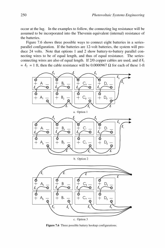
Photovoltaic Systems Engineering250
occur at the lug. In the examples to follow, the connecting lug resistance will beassumed to be incorporated into the Thevenin equivalent (internal) resistance ofthe batteries.
Figure 7.6 shows three possible ways to connect eight batteries in a series-parallel configuration. If the batteries are 12-volt batteries, the system will pro-duce 24 volts. Note that options 1 and 2 show battery-to-battery parallel con-necting wires to be of equal length, and thus of equal resistance. The series-connecting wires are also of equal length. If 2/0 copper cables are used, and if 1= 2 = 1 ft, then the cable resistance will be 0.0000967 Ω for each of these 1-ft
#
#
#
#
#
#
Figure 7.6 Three possible battery hookup configurations.
a. Option 1
b. Option 2
c. Option 3
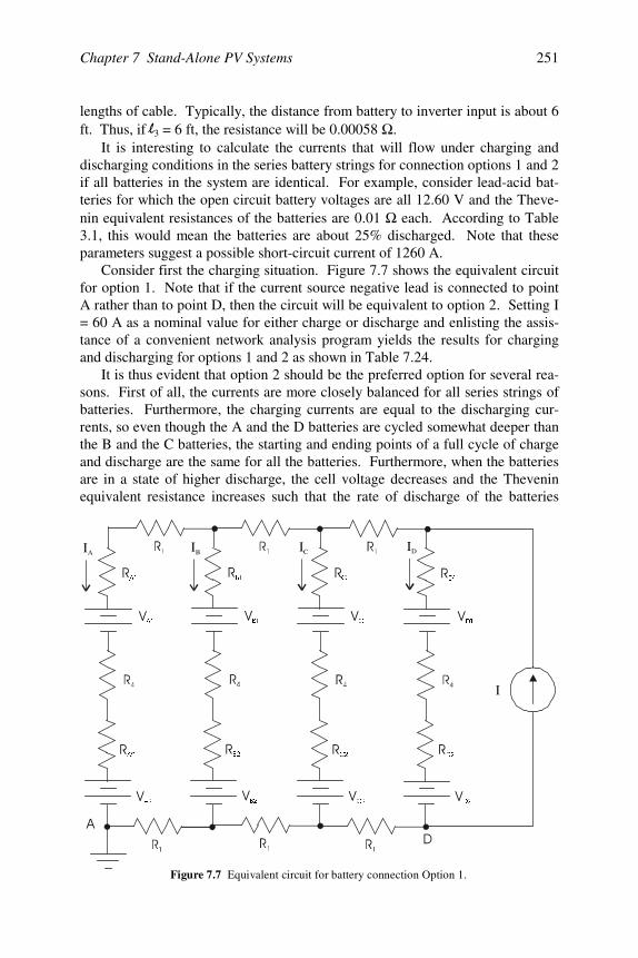
Chapter 7 Stand-Alone PV Systems 251
lengths of cable. Typically, the distance from battery to inverter input is about 6ft. Thus, if 3 = 6 ft, the resistance will be 0.00058 Ω .
It is interesting to calculate the currents that will flow under charging anddischarging conditions in the series battery strings for connection options 1 and 2if all batteries in the system are identical. For example, consider lead-acid bat-teries for which the open circuit battery voltages are all 12.60 V and the Theve-nin equivalent resistances of the batteries are 0.01 Ω each. According to Table3.1, this would mean the batteries are about 25% discharged. Note that theseparameters suggest a possible short-circuit current of 1260 A.
Consider first the charging situation. Figure 7.7 shows the equivalent circuitfor option 1. Note that if the current source negative lead is connected to pointA rather than to point D, then the circuit will be equivalent to option 2. Setting I= 60 A as a nominal value for either charge or discharge and enlisting the assis-tance of a convenient network analysis program yields the results for chargingand discharging for options 1 and 2 as shown in Table 7.24.
It is thus evident that option 2 should be the preferred option for several rea-sons. First of all, the currents are more closely balanced for all series strings ofbatteries. Furthermore, the charging currents are equal to the discharging cur-rents, so even though the A and the D batteries are cycled somewhat deeper thanthe B and the C batteries, the starting and ending points of a full cycle of chargeand discharge are the same for all the batteries. Furthermore, when the batteriesare in a state of higher discharge, the cell voltage decreases and the Theveninequivalent resistance increases such that the rate of discharge of the batteries
$
$
$
$
%
%
%
%
&
'
&
'
&
'
&
'
#
IA IB IC ID
I
Figure 7.7 Equivalent circuit for battery connection Option 1.
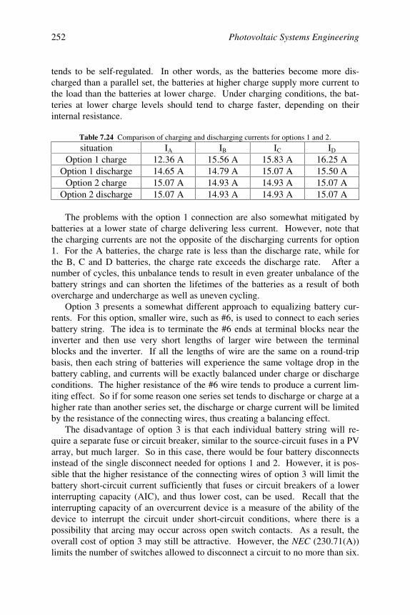
Photovoltaic Systems Engineering252
tends to be self-regulated. In other words, as the batteries become more dis-charged than a parallel set, the batteries at higher charge supply more current tothe load than the batteries at lower charge. Under charging conditions, the bat-teries at lower charge levels should tend to charge faster, depending on theirinternal resistance.
Table 7.24 Comparison of charging and discharging currents for options 1 and 2.
situation IA IB IC ID
Option 1 charge 12.36 A 15.56 A 15.83 A 16.25 AOption 1 discharge 14.65 A 14.79 A 15.07 A 15.50 A
Option 2 charge 15.07 A 14.93 A 14.93 A 15.07 AOption 2 discharge 15.07 A 14.93 A 14.93 A 15.07 A
The problems with the option 1 connection are also somewhat mitigated bybatteries at a lower state of charge delivering less current. However, note thatthe charging currents are not the opposite of the discharging currents for option1. For the A batteries, the charge rate is less than the discharge rate, while forthe B, C and D batteries, the charge rate exceeds the discharge rate. After anumber of cycles, this unbalance tends to result in even greater unbalance of thebattery strings and can shorten the lifetimes of the batteries as a result of bothovercharge and undercharge as well as uneven cycling.
Option 3 presents a somewhat different approach to equalizing battery cur-rents. For this option, smaller wire, such as #6, is used to connect to each seriesbattery string. The idea is to terminate the #6 ends at terminal blocks near theinverter and then use very short lengths of larger wire between the terminalblocks and the inverter. If all the lengths of wire are the same on a round-tripbasis, then each string of batteries will experience the same voltage drop in thebattery cabling, and currents will be exactly balanced under charge or dischargeconditions. The higher resistance of the #6 wire tends to produce a current lim-iting effect. So if for some reason one series set tends to discharge or charge at ahigher rate than another series set, the discharge or charge current will be limitedby the resistance of the connecting wires, thus creating a balancing effect.
The disadvantage of option 3 is that each individual battery string will re-quire a separate fuse or circuit breaker, similar to the source-circuit fuses in a PVarray, but much larger. So in this case, there would be four battery disconnectsinstead of the single disconnect needed for options 1 and 2. However, it is pos-sible that the higher resistance of the connecting wires of option 3 will limit thebattery short-circuit current sufficiently that fuses or circuit breakers of a lowerinterrupting capacity (AIC), and thus lower cost, can be used. Recall that theinterrupting capacity of an overcurrent device is a measure of the ability of thedevice to interrupt the circuit under short-circuit conditions, where there is apossibility that arcing may occur across open switch contacts. As a result, theoverall cost of option 3 may still be attractive. However, the NEC (230.71(A))limits the number of switches allowed to disconnect a circuit to no more than six.
Chapter 7 Stand-Alone PV Systems 253
An interesting approach to this problem is to use 2- or 3-pole circuit breakers,since each device has a single lever for operating the device and hence will countas a single disconnect even though it will disconnect two or three strings of bat-teries with a single flip of the switch handle.
In summary, the key to optimizing battery performance is proper cabling.The use of equal lengths of cables is essential. Problems 7.18–7.20 offer thereader an opportunity to explore the effect of unequal cable lengths and batteryparameters on battery system charging and discharging. Option 2 is clearly bet-ter than option 1 for battery wiring, and option 3 is also potentially attractive.
Furthermore, new batteries tend to have lower internal resistance than olderones of the same type, resulting in greater unbalance of currents in parallelstrings of new batteries. This generally means that if one battery is replaced, allshould be replaced, probably with the exception of an early failure due to a bat-tery defect. In any case, if not all batteries are replaced, the condition of all bat-teries should be carefully checked to ensure that currents are well balanced. Ifthis is not the case, future premature failures may continue to occur. A clamp-ondc ammeter is most useful for this sort of analysis.
7.7 Computer Programs
For the computer wizard or for the person who merely wishes to minimizethe computational effort involved in using a scientific calculator to optimize adesign, a number of useful computer programs are available. From an engi-neering perspective, use of computer programs to assist in system design is es-sential. However, the engineer must have an idea of the limitations of the pro-grams contemplated. The transparency of the computation process may result inthe tendency to let the computer replace the creative thinking process. Hereinlies the liability of computer use.
Fortunately, the computerized computation process need not be transparentto the engineer. By now, after observing the large amount of data presented intabular form in this chapter, the engineer familiar with any spreadsheet programwill quickly observe the utility of a spreadsheet in PV system analysis. In fact,the authors developed their own spreadsheets to perform the analysis of each ofthe systems discussed in this chapter. Generating a customized design worksheetis part of the fun of PV system analysis. It ensures that no part of the analysisprocess is transparent to the system designer.
One area where computer programs can be very useful is the computationallyintensive determination of global radiation on surfaces at arbitrary tilt angles.The tables in Appendix A give data for three tilt angles for each location, but donot necessarily give optimal tilt for any particular system design. This is where aprogram such as NSol! by Orion Energy Corporation can save considerablecomputation time [6]. By varying the tilt and azimuth of the array on a computerkeyboard, it is possible to optimize the match between PV output and systemload requirements.

Photovoltaic Systems Engineering254
Problems
7.1 Offer an explanation for why a collector tilt of latitude+15o gives bettersummer performance in Angola. Check the peak sun hours compilations inAppendix A for other locations to see whether this phenomenon is charac-teristic of any other locations. Comment on the meaning of “su mmer” and“winter” in the tables in Appendix A.
7.2 Assume 10 days of autonomy are desired for a battery system, but the bat-tery size chosen only allows for 9.2 days of storage, with a maximum depthof discharge of 80%. Then assume 12 consecutive days occur duringwhich peak sun averages only 10% of the predicted worst-case average.What will be the state of charge of the battery system after the end of the12th day?
7.3 Under what conditions of system design would the alternate formulationfor battery capacity be used rather than (7.2)? Consider particularly thenumber of days of autonomy required.
7.4. At what ratio of discount rate to inflation rate would the life-cycle costs ofthe 220 Ah and 350 Ah battery systems in the ac refrigerator example inSection 7.2 be the same? Under what economic or other conditions wouldthe purchase of the 350 Ah batteries be justified?
7.5 Calculate the life-cycle costs for the use of the 350 Ah or the 220 Ah bat-teries if the dc refrigerator is used in the example of Section 7.2.
7.6 Calculate the design array current for the ac refrigerator. Then determinethe fuse and disconnect sizes for the array and for the battery system.
7.7 For the ac refrigerator of Section 7.2, determine the number of 4.4A mod-ules that will be needed if tracking mounts are used. Look up the price fora tracking mount for the modules and compare the prices of modules plusmounts for tracking and fixed arrays.
7.8 A battery storage system is to be designed to provide a storage capacity ofsomewhere between 440 and 555 Ah @ 48 V at a C/20 discharge rate.Four battery types are under consideration:
Battery Volts Capacity Type Lifetime Weight Cost EachA 6 220 Ah Flooded 5 yr 56 lb $66B 12 255 Ah agm 8 yr 168 lb $356C 12 180 Ah agm 8 yr 135 lb $301D 12 555 Ah gel 12 yr 564 lb $1941

Chapter 7 Stand-Alone PV Systems 255
Assume i = 2%, d = 5% and a 24-year system lifetime. Perform an LCCfor the four battery types and discuss other considerations that may influ-ence the choice of batteries. If the site were a homeowner, what would yourecommend? Why? If the site were a remote communication system, whatwould you recommend? Why?
7.9 A 500 W, 120 V ac gasoline generator can be purchased for $250 and willgenerate 4 kWh/gal of gasoline at 90% of full load. If the cost of gasolineis $2.00 per gallon, and if the maintenance cycles and costs for the gen-erator are the same as for the generator used in the hybrid system example,determine the LCC of the ac refrigerator system using the generator inplace of the PV modules. The batteries and inverter remain in the system.Assume the generator needs to be replaced every 4 years.
7.10 Tabulate the wire, fuse and switch needs of the ac refrigerator system.Assume the same wire lengths that were used for the dc system.
7.11 Discuss fuse location alternatives in systems and what the fuses will protectfor each location. For example, if a fuse is located at the array vs. at thecontroller, which gives the most system protection?
7.12 In the cabin example, why is a 480-gallon storage tank needed if the pumptakes 7 days to pump the water needed for a 3-day weekend, assuming 160gallon-per-day usage during the weekend?
7.13 Verify the wire size quoted in the text for supplying the two water pumpchoices for the cabin.
7.14 Determine the additional water that can be pumped with excess summerelectricity produced by the cabin array.
7.15 a. Determine the load that can be connected to the entertainment circuitthat will result in a 2% voltage drop in the branch circuit wiring.b. For a 200 W load, determine the wire size that will limit the voltagedrop between distribution panel and load to < 2%.
7.16 Show why the hybrid residence will take 5/8 of 2.9 days to use up 5 hoursof charge at 2250 watts, as claimed in the text.
7.17 Show that the average power consumption in the hybrid residence is 239 Wor less.
7.18 Use a network analysis program to explore the effect of unequal batterycable lengths in the distribution of currents for battery connection options1, 2 and 3 of Figure 7.6. Solve for charging currents and discharging cur-rents of 60 A.

Photovoltaic Systems Engineering256
7.19 Use a network analysis program to explore the effect of unequal open-circuit battery voltages that might be expected for charge levels of 50%and 75%. Assume, for example, that the A batteries of Figure 7.6 arecharged to 50% and the rest of the batteries are charged to 75%. Thensolve for the battery string currents in options 1, 2 and 3 under charge anddischarge conditions.
7.20 Use a network analysis program to explore the effect of unequal internalbattery resistances (Thevenin equivalent resistances) on the charging anddischarging currents for options 1, 2, and 3 of Figure 7.6.
Design Projects
7.21 Develop a spreadsheet or other computer program that will enable com-parative LCC analysis of a stand-alone PV system.
7.22 Extend your program of Problem 7.21 to include hybrid systems.
7.23 Write a program or develop a spreadsheet that will size a pump and wire tothe pump for a PV-powered pumping system if the pumping height anddaily volume are known along with the distance from the array to thepump.
7.24 Design your own little off-grid hide away. Specify your own loads, occu-pancy, peak sun and storage requirements and determine the number ofbatteries and the number of modules you would need to implement thesystem. Then specify BOS components.
7.25 Design you own slightly larger, off-grid hide away for a location at a lati-tude higher than 50°, where winter peak sun hours are significantly lessthan summer peak sun hours. Use winter loads such that your system willend up as a hybrid system.

Chapter 7 Stand-Alone PV Systems 257
References
[1] www.AltEnergystore.com for information on dc refrigerators and other components.[2] Stand-Alone Photovoltaic Systems: A Handbook of Recommended Design Prac-
tices, Sandia National Laboratories, Albuquerque, NM, 1995.[3] www.SouthwestPV.com for information on PV water pumps and other dc loads.[4] www.windsun.com for information on 24 V dc lighting and other dc loads.[5] Danley, D. R., Orion Energy Corporation, Ijamsville, MD, Personal communication
regarding fuel efficiency of fossil fueled generators, August, 1999.[6] "NSol! PV System Sizing Program, V2.8," Orion Energy Corporation, Germantown,
MD, 1993-94.
Suggested Reading
NFPA 70 National Electrical Code, 2002 Edition, National Fire Protection Asso-ciation, Quincy, MA, 2002.
www.batteries4everything.com for battery information.www.unirac.com for information on array mounts.www.zomeworks.com for information on tracking array mounts.

259
Chapter 8UTILITY INTERACTIVE PV SYSTEMS
8.1 Introduction
As the cost of PV systems continues to decrease, utility interactive systemsare becoming more economically viable. Furthermore, increases in consumerawareness correspond to a willingness to pay a premium price for clean electri-cal energy. This feedback loop, coupled with the increased demand for stand-alone systems, has resulted in a healthy demand for PV system components.And this increased demand has enabled PV module and balance of system(BOS) component manufacturers to scale up manufacturing facilities to takeadvantage of economies of scale to further reduce system costs.
In addition to cost reductions, the increased demand for PV systems has ledto significant efforts to improve the reliability of PV system components, de-signs and installations. So not only are PV systems decreasing in cost, but theyare increasing in reliability. While a number of electric utilities have initiatedprograms for installing utility interactive PV systems, the pioneering efforts ofthe Sacramento (California) Municipal Utility District (SMUD) and Austin(Texas) Energy have probably received the most attention in the United States.
SMUD customers participating in the PV Pioneer I program had the optionof paying an extra $4.00/month on their electric bills for which they received a 3to 4 kW PV system installed on their roof. The system takes approximately halfa day to install and is connected to the grid through a separate meter on the util-ity side of the grid, mounted next to the house meter [1]. Nearly 450 SMUDresidential customers were participating in this program in 1998.
A new initiative, PV Pioneer II, enables the customer to own the PV system,with the PV output connected on the customer side of the revenue meter. By2001, SMUD had installed more than 1000 PV systems, including residential,commercial, church and several larger central grid-connected PV systems. Thecombined output of these systems added up to more than 10 MW. In 2001,nearly 2000 SMUD customers signed letters of intent to purchase their own PVsystems. SMUD has the goal of providing 20% of customer energy needs withnonhydro renewable sources by 2011 [2].
Austin (Texas) Energy is promoting the Solar Explorer program. Customersjoin the program by paying an additional $3.50 per month on their electric bills.The additional revenues are used for the construction of larger PV systems thatfeed power into the grid. By 1999, nearly 1000 families, individuals and busi-nesses had signed up with this program, and three larger systems had been in-stalled in conspicuous locations [3].
On December 19, 2001, the New Jersey Board of Public Utilities issued asolicitation for $10 million in renewable energy technology [4]. The bottom lineis that consumers are demanding green energy and many states are responding tothese demands.
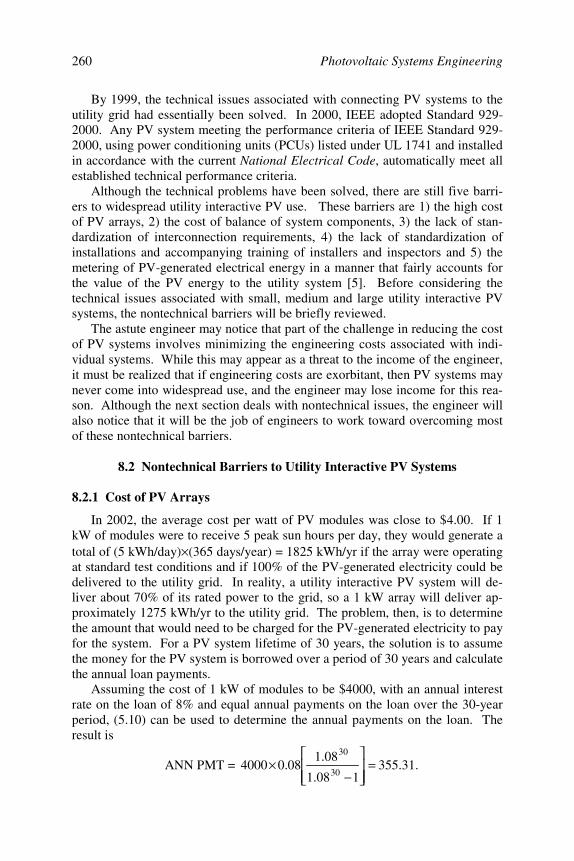
Photovoltaic Systems Engineering260
By 1999, the technical issues associated with connecting PV systems to theutility grid had essentially been solved. In 2000, IEEE adopted Standard 929-2000. Any PV system meeting the performance criteria of IEEE Standard 929-2000, using power conditioning units (PCUs) listed under UL 1741 and installedin accordance with the current National Electrical Code, automatically meet allestablished technical performance criteria.
Although the technical problems have been solved, there are still five barri-ers to widespread utility interactive PV use. These barriers are 1) the high costof PV arrays, 2) the cost of balance of system components, 3) the lack of stan-dardization of interconnection requirements, 4) the lack of standardization ofinstallations and accompanying training of installers and inspectors and 5) themetering of PV-generated electrical energy in a manner that fairly accounts forthe value of the PV energy to the utility system [5]. Before considering thetechnical issues associated with small, medium and large utility interactive PVsystems, the nontechnical barriers will be briefly reviewed.
The astute engineer may notice that part of the challenge in reducing the costof PV systems involves minimizing the engineering costs associated with indi-vidual systems. While this may appear as a threat to the income of the engineer,it must be realized that if engineering costs are exorbitant, then PV systems maynever come into widespread use, and the engineer may lose income for this rea-son. Although the next section deals with nontechnical issues, the engineer willalso notice that it will be the job of engineers to work toward overcoming mostof these nontechnical barriers.
8.2 Nontechnical Barriers to Utility Interactive PV Systems
8.2.1 Cost of PV Arrays
In 2002, the average cost per watt of PV modules was close to $4.00. If 1kW of modules were to receive 5 peak sun hours per day, they would generate atotal of (5 kWh/day) × (365 days/year) = 1825 kWh/yr if the array were operatingat standard test conditions and if 100% of the PV-generated electricity could bedelivered to the utility grid. In reality, a utility interactive PV system will de-liver about 70% of its rated power to the grid, so a 1 kW array will deliver ap-proximately 1275 kWh/yr to the utility grid. The problem, then, is to determinethe amount that would need to be charged for the PV-generated electricity to payfor the system. For a PV system lifetime of 30 years, the solution is to assumethe money for the PV system is borrowed over a period of 30 years and calculatethe annual loan payments.
Assuming the cost of 1 kW of modules to be $4000, with an annual interestrate on the loan of 8% and equal annual payments on the loan over the 30-yearperiod, (5.10) can be used to determine the annual payments on the loan. Theresult is
ANN PMT = .31.355108.1
08.108.04000
30
30
=
−×
Chapter 8 Utility Interactive PV Systems 261
Paying back the loan with no profit would thus require that the annual kWhoutput of the modules would have to be sold for $355.31. This amounts to$355.31 ÷ 1275 kWh = $0.279/kWh. This rate is nearly triple the energy rate ofmost public utilities in the U.S.
Note that the annual rate to be charged is the same regardless of where thePV system is installed. Thus, if installed in an area with an average of 7 peaksun hours, the cost per kWh drops to 5/7 of $0.279/kWh, or $0.199/kWh. Alsonote that since the loan payments will be the same over the life of the loan, thesame rate per kWh can be charged over the lifetime of the system. Dependingupon the inflation rate of utility-generated electricity, it is possible that the priceof utility-generated electricity may at some point in time reach the value of thePV-generated electricity. Problems 1 and 2 provide the opportunity to explorewhat combinations of cost per module, interest rates and loan duration will re-sult in cost-competitive PV electrical energy.
Although the value of PV-generated electrical energy appears to be morethan triple the cost of electricity from the grid, in fact, it is not quite as bad as itmay appear, since the time of day that the electricity is generated adds additionalvalue to the electricity. This observation will be explored in Section 8.2.5.
8.2.2 Cost of Balance of System Components
The cost of PV modules is, of course, only part of the cost of the system.The total system cost also includes all of the array mounts, wiring, surge protec-tion, ground fault protection, the inverter (PCU) and possibly metering or othercomponents that may be required for the interconnection. The installation costalso must be included among the balance of system costs.
In modern systems, most of the protection mechanisms are built into thePCU, so the system can be as simple as the PV array, the PCU, the wiring be-tween the array and PCU and the wiring from the PCU to the point of grid con-nection. Since the grid is essentially the storage mechanism, most of the PVsystem maximum power output can be used, with the exception of system lossesin the wiring, inverter and modules that will normally average about 30%. ThePCU will have maximum power tracking as a feature, so the system will be ca-pable of delivering maximum output power to the grid over almost the entirerange of irradiance to the system.
The economic analysis of the cost of the BOS components follows the sameprocedure as the economic analysis of the cost of the modules. Hence, the cal-culations performed in 8.2.1 must now include the balance of system costs alongwith the PV cost, so the combined cost is still cost competitive. Based on theexperiences of SMUD, there is reason to believe that the BOS costs will alsocontinue to decrease as experience is gained in installation, as larger quantitiesof PCUs are manufactured, as interconnection and installation requirements arestandardized and as a fair value for PV electricity is agreed upon. And, ofcourse, if petroleum becomes more scarce or if global warming is taken seri-ously, the price of fossil generation may rise to the cost of PV generation.
Photovoltaic Systems Engineering262
8.2.3 Standardization of Interconnection Requirements
Two factors dominate the interconnection process: the actual engineeringcosts and the paperwork. The process is further complicated by the fact that thetechnical requirements of utilities vary widely. The solution is straightforward.At this point in time, adequate standards have been developed to cover all of theconcerns. What is thus needed is to educate all parties involved in utility inter-active (grid-connected) PV installations on the validity of the IEEE, UL andNFPA codes and standards so turnkey systems can be installed by qualified in-stallers with minimum engineering costs and minimum paperwork for smallsystems. It is particularly important to eliminate redundant and unnecessaryinterconnection requirements such as separate transformers, redundant relays,unnecessary disconnects and unnecessary meters. Larger systems may requireadditional engineering and paperwork, but these costs will be covered by theincreased amount of energy that will be delivered by these systems.
8.2.4 PV System Installation Considerations
As of 2001, utility interactive PV system installations surpassed stand-alonesystems in annual installed capacity in the U.S. [6]. As of 2002, more than 2000utility interactive systems have been installed, thanks to incentive/buy-downprograms in several states. However, only a handful of installers and inspectorswere familiar with installation requirements. As the costs of PV systems con-tinue to decline and as the costs of fossil-generated electricity continue to in-crease, the need for qualified PV installers and knowledgeable inspectors willvery likely increase significantly.
Fortunately, a small PV installation needs to be installed only where it willnot be shaded, in a manner such that it will not blow away in a strong wind, withhardware that will endure the weather over the lifetime of the system. The pro-cedures for secure roof mounting are well known in the solar domestic waterheating industry and are also applicable to PV roof mounts. Even the tilt of wa-ter heating collectors is comparable to the desirable tilt of PV arrays.
The electrical interconnection requirements for a PV system are relativelyuncomplicated. Thus, electricians need to be taught how to securely mount ar-rays along with the NEC requirements for utility interactive PV installations. Asingle PV installer license could solve the problem, but endorsements to existingelectrical contractor licenses or voluntary certification could also solve theproblem of identifying qualified contractors.
Plans for PV systems can be drawn to include a variety of installation op-tions, so the installer can submit the appropriate installation option for the pro-posed installation.
Finally, the building or electrical inspector needs to be apprised of the sim-plicity of the utility interactive PV system and the permitting process needs to bestreamlined so that reasonable inspection fees can be charged.
Chapter 8 Utility Interactive PV Systems 263
8.2.5 Metering of PV System Output
Metering of the PV system output depends upon whether the PV system isconnected on the load side or the line side of the revenue meter. The NEC(2002) allows for either possibility [7]. If the PV system is connected on theutility side (line side) of the meter, assuming the PV system is owned by theutility, then part of the PV output will be used by the customer, for which thecustomer will be billed by the utility at the standard rate. Another part of the PVoutput will be fed back into the grid if the customer demand is less than the PVsystem output. All this is transparent to the customer and to the utility. Theonly reason for any additional meter to record the PV system generation wouldbe to verify that the PV system is functioning properly. The PCU, however, canbe designed to fulfill this function, so a separate meter is not really needed.
If the PV system is connected on the customer side (load side) of the revenuemeter, the situation changes and depends on whether the system is owned by thecustomer or by the utility. If the utility owns the system, then that fraction of thesystem output that is used by the customer does not register on the revenue me-ter. If there is excess PV energy, it feeds into the grid and may cause the reve-nue meter to run backward. Obviously this presents a more complicated situa-tion for the utility to determine the customer usage and appropriate charges tothe customer.
On the other hand, if the customer owns the PV system that is connected onthe load side of the meter, then the customer’s energy needs are first supplied bythe PV system, with any additional demand being supplied by the utility. Forthat fraction of PV energy used by the PV system owner, the effect on the me-tering is equivalent to an energy conservation measure the meter simply reg-isters a lower amount of consumption. Since the system has no storage provi-sions, if the PV system output exceeds the demand of the owner, the excess out-put is transferred to the grid, possibly causing the meter to run backward. Thequestion then arises as to whether the customer should donate this extra electric-ity to the utility or should be compensated for it.
The Public Utility Regulatory Policies Act of 1978 (PURPA) [8] requiresthat the utility pay for this electricity at the rate of its avoided cost. However,the avoided cost figure is generally established as the utility’s wholesale cost ofelectricity, which may be significantly below the retail rate paid by the customerif an average figure is used. Furthermore, if the utility chooses to pay avoidedcost, a separate metering scheme is needed to monitor that part of the PV outputthat is returned to the utility. Such a metering scheme adds to the cost of theinstallation, especially if it incorporates a time of day component.
To eliminate this added complication, more than two-thirds of the states haveenacted net metering requirements. Net metering simply means that the utilitypays the customer at the retail rate for electricity generated by the customer. Netmetering makes sense because it simplifies the meter connection and the corre-sponding installation cost. It also provides an incentive for installation of PVsystems as well as other distributed generation sources, such as wind generators.
Photovoltaic Systems Engineering264
Net metering for PV systems makes additional sense because the utilityelectricity displaced by PV systems is generally of high value, because it is pro-duced during utility peaking time when more expensive utility generation isbrought on line to meet utility demand. As long as the price paid by the utilityfor the PV output is less than the marginal cost of peaking electricity, the utilitystill ends up profiting by selling the electricity at its acquisition cost.
Finally, net metering makes sense because distributed generation from PVsystems reduces the utility load on its transmission and distribution lines. Thiscan reduce the need for upgrading these lines to meet increased customer load.
Currently, peak demand is generally met by utilities with gas turbine peakinggenerators that can be brought on line quickly. These generators are typicallyused less than 10% of the time to meet system peak load requirements. Al-though these systems are less costly on a per kW basis than large fossil or nu-clear plants, the cost per kWh from these systems is quite high.
Consider, for example, a 1 MW system that has an initial cost of $500,000.At an 8% lending rate, the annual payments on this system on a 20-year loanwill be $50,929. If the system operates 5% of the time at full load, it will gener-ate 0.05 × (1000 kW) × (24 hr/day) × (365 days/year) = 438,000 kWh/yr. Thisamounts to a cost of $0.12/kWh just to cover the cost of the loan. Fuel for gasturbine engines can add another $0.10/kWh as an operating cost, so even ifmaintenance is not included, the marginal cost of peaking electricity is seen tobe more than $0.20/kWh. Thus, if a utility ends up paying $0.09/kWh as retailrate for PV generation, it is likely avoiding a cost of $0.20/kWh or more, espe-cially if the PV system displaces the initial capitalization of the gas turbine gen-eration system.
Displacing the need for the gas turbine is also an interesting consideration.What this means is that the PV system will be in operation when it is needed.This, of course, means that the PV system will be needed during peak sun hoursand that the PV system will be on line during peak sun hours. Since in manyareas utility demand is due to air conditioning at or near peak sun time, the firstrequirement is fulfilled. The second requirement is fulfilled if the PV systemoperates reliably every day of the year. In fact, when the value of electricity isconsidered, orientation of the array toward the west may result in better trackingof utility peak times by the PV output. Even though total kWh production maybe less, as was noted at the end of Chapter 2 and illustrated in Figure 2.14, theoverall value of the energy generated during peak hours may exceed the value ofthe energy generated by a directly south-facing array.
8.3 Technical Considerations for Connecting to the Grid
8.3.1 Introduction
As noted in Chapter 3, IEEE Standard 929-2000 has been developed to ad-dress the technical issues associated with utility interactive PV systems. Thestandard sets limits for voltage disturbances, frequency disturbances, islandingprotection, power factor, harmonic distortion, reconnect after grid failure andrestoration, injection of dc into the ac system, grounding and disconnects.
Chapter 8 Utility Interactive PV Systems 265
The quality of the output of the PCU was discussed briefly in Chapter 3.IEEE 929-2000 [9] refers to other earlier standards that were developed to insurethat power supplied to the grid by small power producers meets certain stan-dards for frequency, harmonic content and voltage level. The primary concernof IEEE 929-2000 is to guarantee that the PCU will disconnect from the utilitygrid if the grid loses power or strays outside established limits for voltage orfrequency, even if other PV sources are connected to the grid.
UL 1741 [10] prescribes a test procedure to verify that the PCU will discon-nect properly from the grid under prescribed conditions of grid voltage and fre-quency. Thus, any PCU listed under UL 1741 has been tested to meet the crite-ria established in IEEE 929.
When considering the connection of a PV source to the grid, it is importantto distinguish between the electrical characteristics of a PCU and a conventionalrotating generator. First of all, most utility interactive PCUs are best modeled asdependent current sources, while rotating generators appear as voltage sources.In the event of a short-circuit fault, a rotating generator can deliver a very largecurrent, limited only by the ability of the prime mover to keep the generator ro-tating. Any energy stored as rotational energy can be dissipated into a shortcircuit as electrical energy. On the other hand, if a short circuit occurs at theoutput of a PCU, little more current than full-load value will flow from the PCU.
Because the PCU acts as a current source, it is easier to ensure that the PCUwill meet the standards for utility interconnection. The reason is that the utilityis close to being an ideal voltage source. Hence, the PCU can sense the utilityvoltage and frequency and inject current only if the voltage and frequency fallwithin prescribed limits. This same circuitry can be used to ensure that the cur-rent is injected in phase with the utility voltage. This assures a high power fac-tor for the PCU output. The sensing circuitry has high impedance inputs andcan remain connected to the utility at all times in order to monitor the voltageand frequency stability of the utility.
In addition to the areas of concern to utilities in IEEE 929-2000, the NECaddresses areas that relate to the safety and performance of the system from theperspective of the owner, assuming the PV system to be customer-owned andconnected on the load side of the revenue meter.
The reader should keep in mind that utility interactive inverters are almostalways based on conversion technology controlled by a microcontroller. Nonu-tility interactive units do not need nearly as sophisticated circuitry to satisfy gridconnection concerns and may be based on other technologies, as discussed inChapter 3. The microcontroller, in association with sensing circuitry, is able tomeasure and control many parameters associated with PCU performance.
8.3.2 IEEE Standard 929-2000 Issues
Voltage DisturbancesTable 8.1 shows voltage levels and trip times as listed in IEEE 929-2000 [9].
The voltage levels are based on limits established by ANSI C84.1 for a nominal120 V base voltage. The percentages listed apply to other base voltage levels.
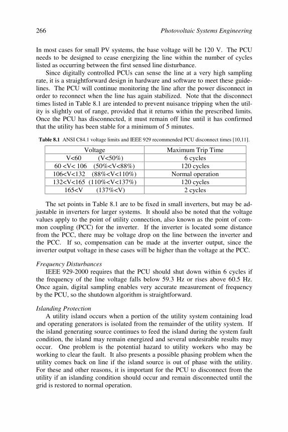
Photovoltaic Systems Engineering266
In most cases for small PV systems, the base voltage will be 120 V. The PCUneeds to be designed to cease energizing the line within the number of cycleslisted as occurring between the first sensed line disturbance.
Since digitally controlled PCUs can sense the line at a very high samplingrate, it is a straightforward design in hardware and software to meet these guide-lines. The PCU will continue monitoring the line after the power disconnect inorder to reconnect when the line has again stabilized. Note that the disconnecttimes listed in Table 8.1 are intended to prevent nuisance tripping when the util-ity is slightly out of range, provided that it returns within the prescribed limits.Once the PCU has disconnected, it must remain off line until it has confirmedthat the utility has been stable for a minimum of 5 minutes.
Table 8.1 ANSI C84.1 voltage limits and IEEE 929 recommended PCU disconnect times [10,11].
Voltage Maximum Trip TimeV<60 (V<50%) 6 cycles
60 <V< 106 (50%<V<88%) 120 cycles106<V<132 (88%<V<110%) Normal operation132<V<165 (110%<V<137%) 120 cycles
165<V (137%<V) 2 cycles
The set points in Table 8.1 are to be fixed in small inverters, but may be ad-justable in inverters for larger systems. It should also be noted that the voltagevalues apply to the point of utility connection, also known as the point of com-mon coupling (PCC) for the inverter. If the inverter is located some distancefrom the PCC, there may be voltage drop on the line between the inverter andthe PCC. If so, compensation can be made at the inverter output, since theinverter output voltage in these cases will be higher than the voltage at the PCC.
Frequency DisturbancesIEEE 929-2000 requires that the PCU should shut down within 6 cycles if
the frequency of the line voltage falls below 59.3 Hz or rises above 60.5 Hz.Once again, digital sampling enables very accurate measurement of frequencyby the PCU, so the shutdown algorithm is straightforward.
Islanding ProtectionA utility island occurs when a portion of the utility system containing load
and operating generators is isolated from the remainder of the utility system. Ifthe island generating source continues to feed the island during the system faultcondition, the island may remain energized and several undesirable results mayoccur. One problem is the potential hazard to utility workers who may beworking to clear the fault. It also presents a possible phasing problem when theutility comes back on line if the island source is out of phase with the utility.For these and other reasons, it is important for the PCU to disconnect from theutility if an islanding condition should occur and remain disconnected until thegrid is restored to normal operation.
Chapter 8 Utility Interactive PV Systems 267
Normally, a single PCU will readily disconnect from the utility in the eventof an islanding condition. The reason is simply that the load of the island willalmost always be far more than the PCU can supply. As a result, the PCU ter-minal voltage will drop below the trip limits or the PCU current will exceed itsrated value and the PCU will disconnect from the utility.
The greatest concern over islanding occurs when more than one PCU is inoperation within the island. In this case, it is possible that they will support afeedback situation in which each PCU, sensing the combined output of the otherPCUs, thinks the output of the other PCUs constitutes the grid. This possibilityis enhanced under worst-case load conditions. It is thus useful to consider whatmight constitute worst-case load conditions.
Worst-case load conditions occur if, when the island is created by the utilityfault, the island voltage does not change quickly to steady-state fault value. Thiswill occur under two conditions: resonance at the utility frequency and islandmotor loads with low damping, such as grinding wheels, that continue to rotateeven though power is removed from the motor.
If a circuit is at resonance with a relatively high Q, then it will continue tooscillate at its natural resonant frequency until the oscillation is ultimatelydamped out. As long as a motor continues to rotate, it will act as a generatorand return its back emf to the grid. While induction motors are normally ineffi-cient generators, synchronous motors are very efficient generators. The genera-tion frequency, of course, depends on the rotation speed, so as the motor slowsdown, the generated frequency changes.
Circuit analysis textbooks generally prove that any parallel RLC circuit willbe underdamped if it has a Q>0.5. Equation (8.1) represents the response of anunderdamped parallel RLC circuit.
)tcos(eV)t(v dt
m φ+ω= α− , (8.1)
where Vm is the initial amplitude, RC2
1=α , LC
1o =ω , 22
od α−ω=ω and
φ is a phase angle that depends upon initial energy storage in the inductor andcapacitor. The Q of the circuit can be found from
RC2
Q oo ω=α
ω= (8.2)
It is interesting to use (8.1) and (8.2) to calculate how long it will take for theamplitude of the voltage to decrease to the PCU trip limit as a function of Q.
The two important parameters of the equation are the exponentially decayingamplitude part, Vme W, and the natural frequency, d. Assuming the energizedgrid has a natural resonant frequency outside the trip limits, the PCU will sensethe frequency departure and disconnect within the prescribed time. If the naturalresonant frequency is within the trip limits, then the PCU will need to disconnectwhen the voltage falls outside the trip limits. For the case of the motor/flywheel
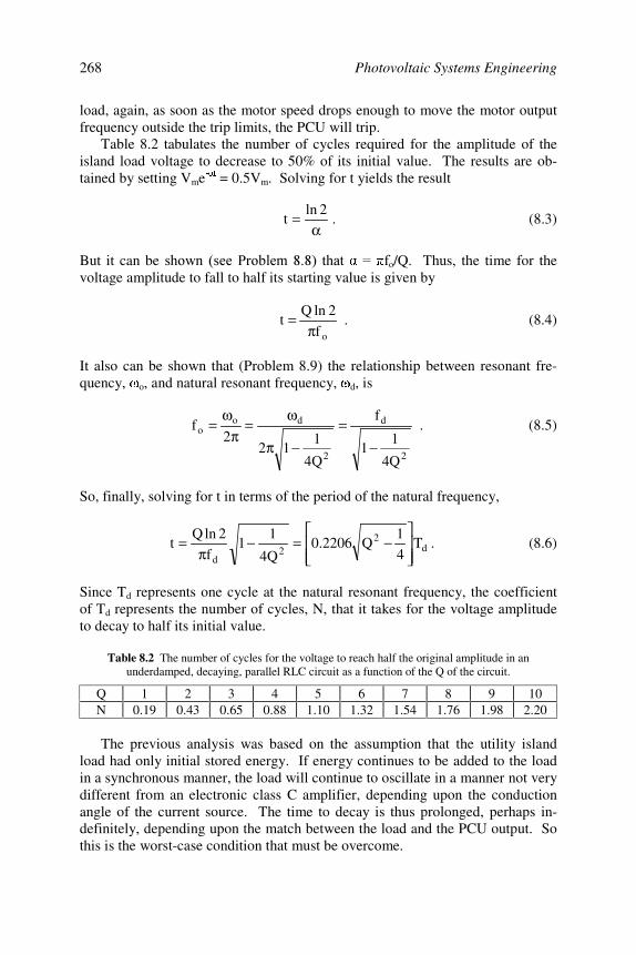
Photovoltaic Systems Engineering268
load, again, as soon as the motor speed drops enough to move the motor outputfrequency outside the trip limits, the PCU will trip.
Table 8.2 tabulates the number of cycles required for the amplitude of theisland load voltage to decrease to 50% of its initial value. The results are ob-tained by setting Vme W = 0.5Vm. Solving for t yields the result
α= 2ln
t . (8.3)
But it can be o/Q. Thus, the time for thevoltage amplitude to fall to half its starting value is given by
of2lnQ
tπ
= . (8.4)
It also can be shown that (Problem 8.9) the relationship between resonant fre-quency, o, and natural resonant frequency, d, is
2
d
2
doo
Q4
11
f
Q4
112
2f
−=
−π
ω=
πω
= . (8.5)
So, finally, solving for t in terms of the period of the natural frequency,
d2
2d
T41
Q2206.0Q4
11
f2lnQ
t
−=−
π= . (8.6)
Since Td represents one cycle at the natural resonant frequency, the coefficientof Td represents the number of cycles, N, that it takes for the voltage amplitudeto decay to half its initial value.
Table 8.2 The number of cycles for the voltage to reach half the original amplitude in anunderdamped, decaying, parallel RLC circuit as a function of the Q of the circuit.
Q 1 2 3 4 5 6 7 8 9 10N 0.19 0.43 0.65 0.88 1.10 1.32 1.54 1.76 1.98 2.20
The previous analysis was based on the assumption that the utility islandload had only initial stored energy. If energy continues to be added to the loadin a synchronous manner, the load will continue to oscillate in a manner not verydifferent from an electronic class C amplifier, depending upon the conductionangle of the current source. The time to decay is thus prolonged, perhaps in-definitely, depending upon the match between the load and the PCU output. Sothis is the worst-case condition that must be overcome.
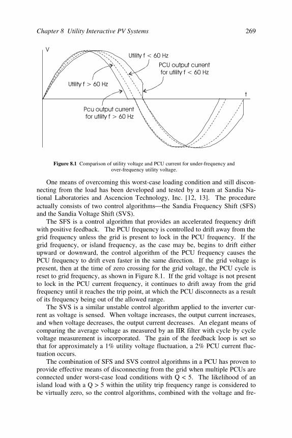
Chapter 8 Utility Interactive PV Systems 269
One means of overcoming this worst-case loading condition and still discon-necting from the load has been developed and tested by a team at Sandia Na-tional Laboratories and Ascencion Technology, Inc. [12, 13]. The procedureactually consists of two control algorithms the Sandia Frequency Shift (SFS)and the Sandia Voltage Shift (SVS).
The SFS is a control algorithm that provides an accelerated frequency driftwith positive feedback. The PCU frequency is controlled to drift away from thegrid frequency unless the grid is present to lock in the PCU frequency. If thegrid frequency, or island frequency, as the case may be, begins to drift eitherupward or downward, the control algorithm of the PCU frequency causes thePCU frequency to drift even faster in the same direction. If the grid voltage ispresent, then at the time of zero crossing for the grid voltage, the PCU cycle isreset to grid frequency, as shown in Figure 8.1. If the grid voltage is not presentto lock in the PCU current frequency, it continues to drift away from the gridfrequency until it reaches the trip point, at which the PCU disconnects as a resultof its frequency being out of the allowed range.
The SVS is a similar unstable control algorithm applied to the inverter cur-rent as voltage is sensed. When voltage increases, the output current increases,and when voltage decreases, the output current decreases. An elegant means ofcomparing the average voltage as measured by an IIR filter with cycle by cyclevoltage measurement is incorporated. The gain of the feedback loop is set sothat for approximately a 1% utility voltage fluctuation, a 2% PCU current fluc-tuation occurs.
The combination of SFS and SVS control algorithms in a PCU has proven toprovide effective means of disconnecting from the grid when multiple PCUs areconnected under worst-case load conditions with Q < 5. The likelihood of anisland load with a Q > 5 within the utility trip frequency range is considered tobe virtually zero, so the control algorithms, combined with the voltage and fre-
Figure 8.1 Comparison of utility voltage and PCU current for under-frequency andover-frequency utility voltage.
Photovoltaic Systems Engineering270
quency trip limits, provide effective anti-islanding protection for the PCUs.Multiple field tests by Sandia and Ascencion Technology have verified the va-lidity of these control algorithms for both resonant and motor loads.
Since the PCU sensing circuitry is not disconnected from the grid, when thegrid is restored, the PCU is capable of monitoring the grid voltage and frequencyfor the time specified by IEEE 929-2000. The PCU is then either immediatelyreconnected at full capacity or gradually brought up to full capacity, dependingon the PCU output control algorithm.
Power FactorThe rule here is simple. The PCU must operate at a power factor greater
than 0.85 leading or lagging. With utility approval, it may be acceptable to op-erate at a leading power factor less than 0.85 to compensate for utility or build-ing lagging power factor. This condition is easily monitored by the PCU, sincevoltage and current are being sensed for other purposes. It should be noted thatthe power factor is defined at the fundamental frequency for nonsinusoidal cur-rent delivered by the PCU.
Reconnect after Grid Failure and RestorationIEEE 929-2000 recommends a 5-minute delay after utility grid power is re-
stored before reconnecting the PCU to the grid. Since this is a software func-tion, the PCU can be programmed to reconnect at any point in time the currentversion of IEEE 929 may require. The reason for the wait is to avoid a recurringconnect/disconnect condition. Often utilities employ automatic reclosers to re-store service. Many utility faults clear themselves in a short time, such as whensomething falls across the lines and is burned by I2R heating. But other faults,such as downed lines resulting from accident or storm, remain faulted as therecloser tries to reset the circuit a second and a third time. If the fault remains,the utility should remain disconnected. Thus, it is desirable to have the utilitygrid operate in the normal range for sufficient time to ensure stability prior toreestablishing connection to the PCU.
Injection of dc Into the ac SystemThe PCU should not inject dc current into the ac system in excess of 0.5% of
its rated ac output current under any PCU operating conditions. A number ofmeans of preventing dc injection are available to the PCU designer. The pri-mary reason for keeping dc out of the grid is its effect on inductive loads. Witha combination of dc and ac applied to many inductors, the inductor may bedriven into saturation, resulting in hysteresis losses beyond the device rating.Transformer coupling is one way to keep dc from being coupled to the grid, butit is expensive and unnecessary in view of less costly, equally reliable, otherdesign options. Since the inverter monitors its current, it can be programmed toshut down if it should develop excessive dc in its output.
GroundingIEEE 929-2000 recommends that the PCU and PV system be grounded in
accordance with applicable codes. Grounding has been discussed in several
Chapter 8 Utility Interactive PV Systems 271
previous examples and will again be discussed in Section 8.3.3. Perhaps a re-minder is in order that in the U.S., for systems operating over 50 V, one of thecurrent-carrying conductors must be grounded. Grounding conductors, on theother hand, do not carry current under normal system operation, but connect thesystem or parts of the system to the system ground. Grounding conductors doconduct current when a ground fault occurs. The grounding conductor is thefamiliar round terminal on three-prong 120 V attachment caps (plug). Thegrounding wire is the bare wire or the green wire in electrical distribution sys-tems, which is ultimately connected to a water pipe or a ground rod system.
DisconnectsA utility interface disconnect switch is a manual, lockable, load-break dis-
connect switch that is visible to and accessible to utility workers. It can be veri-fied from a distance that the switch is open. Some utilities require such switchesat the point of connection of the PV system to the utility to assure utility workersthat the PV system has been disconnected. At this point, however, suchswitches are redundant, since any system installed in accordance with the NECwill have an anti-islanding inverter that will shut down when the utility is down.Furthermore, in the event that many PV systems should be connected to the grid,manually disconnecting and manually locking out all the systems will becomeunnecessarily time-consuming. Simply following standard grounding proceduresprior to working on lines eliminates any need for manual PV disconnects. It ispossible that, as utility interactive PV penetration increases, PCUs will be con-trollable via power line carrier signals similar to those currently in use by manyutilities for demand side management purposes.
8.3.3 National Electrical Code Considerations
The National Electrical Code [7] is an important source of information to thePV design engineer, since it clearly defines acceptable PV system design prac-tice. Article 690 deals exclusively with PV systems, but refers to other articlessuch as Article 240 on overcurrent devices, Article 250 on grounding and Arti-cle 310 on conductor ampacities. Other parts of the NEC also apply to specificinstallations or installation methods. Table 8.3 summarizes the components ofNEC Article 690 and lists some of the other NEC articles that apply to PV sys-tem installations.
Most of the subsections of Article 690 are self-explanatory, so they will beleft as essential pleasure reading for the reader who will be designing a PV sys-tem. A few points, however, are worthy of additional comment. The readershould realize that the intent of the following discussion is to highlight certainportions of the NEC. The serious system designer should consult a more com-prehensive reference, such as Sand2001-0674 by John Wiles [14].
Grounding and Source CircuitsArticle 690.4(c) requires that “connections to a module or pane l shall be ar-
ranged so that removal of a module or panel from a photovoltaic source circuitdoes not interrupt a grounded conductor to another photovoltaic source circuit.
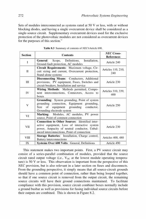
Photovoltaic Systems Engineering272
Sets of modules interconnected as systems rated at 50 V or less, with or withoutblocking diodes, and having a single overcurrent device shall be considered as asingle-source circuit. Supplementary overcurrent devices used for the exclusiveprotection of the photovoltaic modules are not considered as overcurrent devicesfor the purposes of this section.”
Table 8.3 Summary of contents of NEC Article 690.
Section Contents NEC Cross-References
IGeneral: Scope, Definitions, Installation,Ground-fault protection, AC modules
Article 240
IICircuit Requirements: Maximum voltage, Cir-cuit sizing and current, Overcurrent protection,Stand-alone systems
Articles 110, 210,240
IIIDisconnecting Means: Conductors, Additionalprovisions, PV equipment, Fuses, Switches andcircuit breakers, Installation and service
Article 230
IVWiring Methods: Methods permitted, Compo-nent interconnections, Connectors, Access toboxes
Articles 310, 339,400
V
Grounding: System grounding, Point of systemgrounding connection, Equipment grounding,Size of equipment grounding conductor,Grounding electrode system
Article 250
VIMarking: Modules, AC modules, PV powersource, Point of common connection
VII
Connection to Other Sources: Identified inter-active equipment, Loss of interactive systempower, Ampacity of neutral conductor, Unbal-anced interconnections, Point of connection
Article 230
VIIIStorage Batteries: Installation, Charge control,Battery interconnections
Articles 400, 480
IX Systems Over 600 Volts: General, Definitions Article 490
This statement makes two important points. First, a PV source circuit mayconsist of a series-parallel combination of modules, provided that the sourcecircuit rated output voltage (i.e., VOC at the lowest module operating tempera-ture) is 50 V or less. This observation is important from the perspective of thisNEC provision, but is also relevant in a later section on fuses and disconnects.From the grounding perspective, it simply means that all source-circuit groundsshould have a common point of connection, rather than being looped together,so that if one source circuit is removed from the output circuit, the remainingsource circuits will have their ground connections maintained. To facilitatecompliance with this provision, source circuit combiner boxes normally includea ground busbar as well as provisions for fusing individual source circuits beforetheir outputs are combined. This is shown in Figure 8.2.
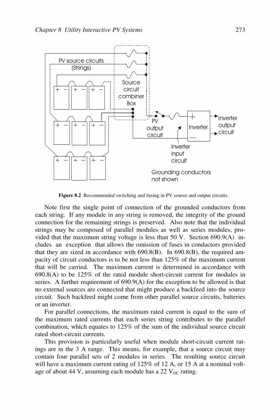
Chapter 8 Utility Interactive PV Systems 273
Note first the single point of connection of the grounded conductors fromeach string. If any module in any string is removed, the integrity of the groundconnection for the remaining strings is preserved. Also note that the individualstrings may be composed of parallel modules as well as series modules, pro-vided that the maximum string voltage is less than 50 V. Section 690.9(A) in-cludes an exception that allows the omission of fuses in conductors providedthat they are sized in accordance with 690.8(B). In 690.8(B), the required am-pacity of circuit conductors is to be not less than 125% of the maximum currentthat will be carried. The maximum current is determined in accordance with690.8(A) to be 125% of the rated module short-circuit current for modules inseries. A further requirement of 690.9(A) for the exception to be allowed is thatno external sources are connected that might produce a backfeed into the sourcecircuit. Such backfeed might come from other parallel source circuits, batteriesor an inverter.
For parallel connections, the maximum rated current is equal to the sum ofthe maximum rated currents that each series string contributes to the parallelcombination, which equates to 125% of the sum of the individual source circuitrated short-circuit currents.
This provision is particularly useful when module short-circuit current rat-ings are in the 3 A range. This means, for example, that a source circuit maycontain four parallel sets of 2 modules in series. The resulting source circuitwill have a maximum current rating of 125% of 12 A, or 15 A at a nominal volt-age of about 44 V, assuming each module has a 22 VOC rating.
!"
Figure 8.2 Recommended switching and fusing in PV source and output circuits.
#$%&
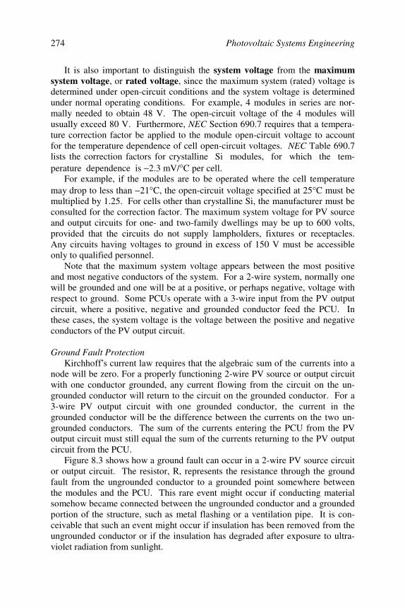
Photovoltaic Systems Engineering274
It is also important to distinguish the system voltage from the maximumsystem voltage, or rated voltage, since the maximum system (rated) voltage isdetermined under open-circuit conditions and the system voltage is determinedunder normal operating conditions. For example, 4 modules in series are nor-mally needed to obtain 48 V. The open-circuit voltage of the 4 modules willusually exceed 80 V. Furthermore, NEC Section 690.7 requires that a tempera-ture correction factor be applied to the module open-circuit voltage to accountfor the temperature dependence of cell open-circuit voltages. NEC Table 690.7lists the correction factors for crystalline Si modules, for which the tem-perature dependence is −2.3 mV/°C per cell.
For example, if the modules are to be operated where the cell temperaturemay drop to less than −21°C, the open-circuit voltage specified at 25°C must bemultiplied by 1.25. For cells other than crystalline Si, the manufacturer must beconsulted for the correction factor. The maximum system voltage for PV sourceand output circuits for one- and two-family dwellings may be up to 600 volts,provided that the circuits do not supply lampholders, fixtures or receptacles.Any circuits having voltages to ground in excess of 150 V must be accessibleonly to qualified personnel.
Note that the maximum system voltage appears between the most positiveand most negative conductors of the system. For a 2-wire system, normally onewill be grounded and one will be at a positive, or perhaps negative, voltage withrespect to ground. Some PCUs operate with a 3-wire input from the PV outputcircuit, where a positive, negative and grounded conductor feed the PCU. Inthese cases, the system voltage is the voltage between the positive and negativeconductors of the PV output circuit.
Ground Fault ProtectionKirchhoff’s current law requires that the algebraic sum of the currents into a
node will be zero. For a properly functioning 2-wire PV source or output circuitwith one conductor grounded, any current flowing from the circuit on the un-grounded conductor will return to the circuit on the grounded conductor. For a3-wire PV output circuit with one grounded conductor, the current in thegrounded conductor will be the difference between the currents on the two un-grounded conductors. The sum of the currents entering the PCU from the PVoutput circuit must still equal the sum of the currents returning to the PV outputcircuit from the PCU.
Figure 8.3 shows how a ground fault can occur in a 2-wire PV source circuitor output circuit. The resistor, R, represents the resistance through the groundfault from the ungrounded conductor to a grounded point somewhere betweenthe modules and the PCU. This rare event might occur if conducting materialsomehow became connected between the ungrounded conductor and a groundedportion of the structure, such as metal flashing or a ventilation pipe. It is con-ceivable that such an event might occur if insulation has been removed from theungrounded conductor or if the insulation has degraded after exposure to ultra-violet radiation from sunlight.
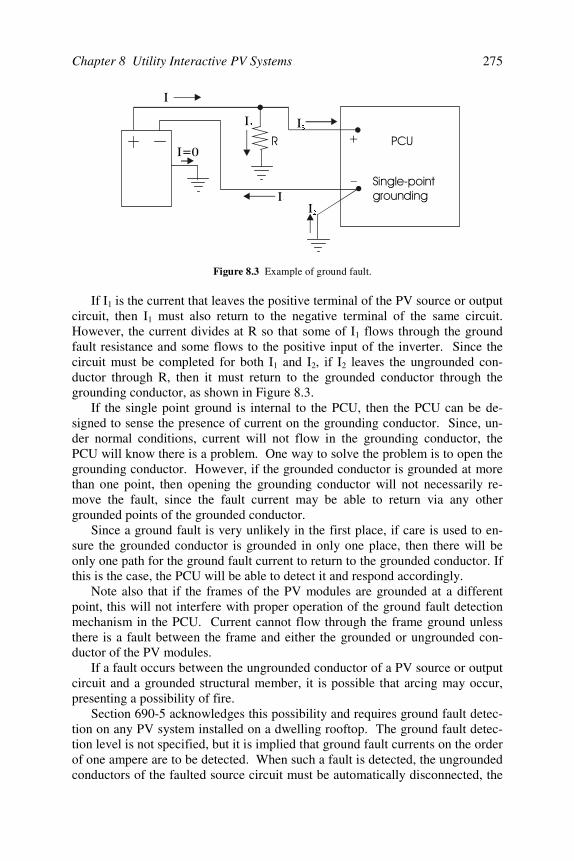
Chapter 8 Utility Interactive PV Systems 275
If I1 is the current that leaves the positive terminal of the PV source or outputcircuit, then I1 must also return to the negative terminal of the same circuit.However, the current divides at R so that some of I1 flows through the groundfault resistance and some flows to the positive input of the inverter. Since thecircuit must be completed for both I1 and I2, if I2 leaves the ungrounded con-ductor through R, then it must return to the grounded conductor through thegrounding conductor, as shown in Figure 8.3.
If the single point ground is internal to the PCU, then the PCU can be de-signed to sense the presence of current on the grounding conductor. Since, un-der normal conditions, current will not flow in the grounding conductor, thePCU will know there is a problem. One way to solve the problem is to open thegrounding conductor. However, if the grounded conductor is grounded at morethan one point, then opening the grounding conductor will not necessarily re-move the fault, since the fault current may be able to return via any othergrounded points of the grounded conductor.
Since a ground fault is very unlikely in the first place, if care is used to en-sure the grounded conductor is grounded in only one place, then there will beonly one path for the ground fault current to return to the grounded conductor. Ifthis is the case, the PCU will be able to detect it and respond accordingly.
Note also that if the frames of the PV modules are grounded at a differentpoint, this will not interfere with proper operation of the ground fault detectionmechanism in the PCU. Current cannot flow through the frame ground unlessthere is a fault between the frame and either the grounded or ungrounded con-ductor of the PV modules.
If a fault occurs between the ungrounded conductor of a PV source or outputcircuit and a grounded structural member, it is possible that arcing may occur,presenting a possibility of fire.
Section 690-5 acknowledges this possibility and requires ground fault detec-tion on any PV system installed on a dwelling rooftop. The ground fault detec-tion level is not specified, but it is implied that ground fault currents on the orderof one ampere are to be detected. When such a fault is detected, the ungroundedconductors of the faulted source circuit must be automatically disconnected, the
' (
)
*
Figure 8.3 Example of ground fault.
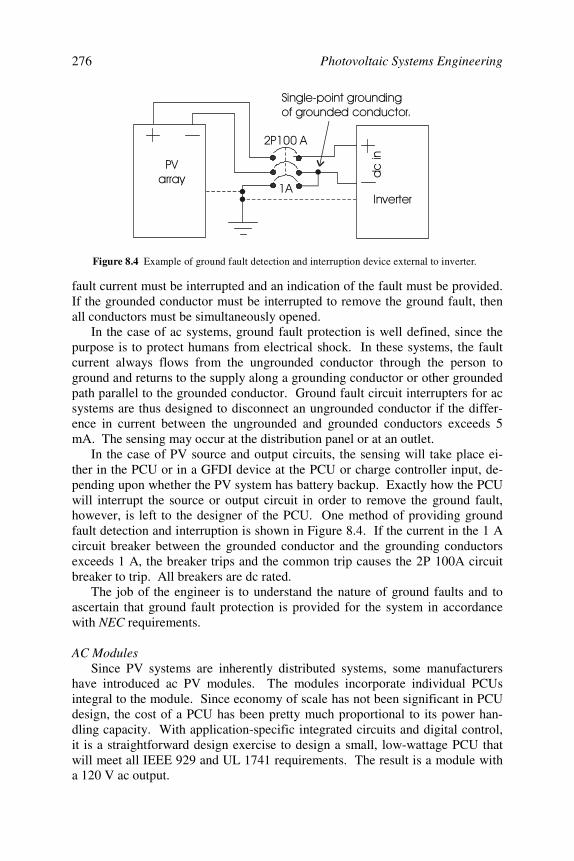
Photovoltaic Systems Engineering276
fault current must be interrupted and an indication of the fault must be provided.If the grounded conductor must be interrupted to remove the ground fault, thenall conductors must be simultaneously opened.
In the case of ac systems, ground fault protection is well defined, since thepurpose is to protect humans from electrical shock. In these systems, the faultcurrent always flows from the ungrounded conductor through the person toground and returns to the supply along a grounding conductor or other groundedpath parallel to the grounded conductor. Ground fault circuit interrupters for acsystems are thus designed to disconnect an ungrounded conductor if the differ-ence in current between the ungrounded and grounded conductors exceeds 5mA. The sensing may occur at the distribution panel or at an outlet.
In the case of PV source and output circuits, the sensing will take place ei-ther in the PCU or in a GFDI device at the PCU or charge controller input, de-pending upon whether the PV system has battery backup. Exactly how the PCUwill interrupt the source or output circuit in order to remove the ground fault,however, is left to the designer of the PCU. One method of providing groundfault detection and interruption is shown in Figure 8.4. If the current in the 1 Acircuit breaker between the grounded conductor and the grounding conductorsexceeds 1 A, the breaker trips and the common trip causes the 2P 100A circuitbreaker to trip. All breakers are dc rated.
The job of the engineer is to understand the nature of ground faults and toascertain that ground fault protection is provided for the system in accordancewith NEC requirements.
AC ModulesSince PV systems are inherently distributed systems, some manufacturers
have introduced ac PV modules. The modules incorporate individual PCUsintegral to the module. Since economy of scale has not been significant in PCUdesign, the cost of a PCU has been pretty much proportional to its power han-dling capacity. With application-specific integrated circuits and digital control,it is a straightforward design exercise to design a small, low-wattage PCU thatwill meet all IEEE 929 and UL 1741 requirements. The result is a module witha 120 V ac output.
++
,-
. ,-
Figure 8.4 Example of ground fault detection and interruption device external to inverter.
* /
Chapter 8 Utility Interactive PV Systems 277
The main advantage of ac modules is that they allow the system to be built inincrements according to needs and budget. The main disadvantage is that eachmodule inverter requires separate intelligence and control, increasing the cost ofthe system somewhat.
Other advantages include on board maximum power tracking and a 120 V acoutput circuit that carries correspondingly less current, enabling wiring withsmaller wire sizes with minimal voltage drop. The output of an ac module isthus considered to be an inverter output circuit and none of the dc source circuitand output circuit rules that apply to dc modules apply to ac modules. A singledisconnect is allowed for the combined parallel ac output of more than one acmodule, but each module must have its own connector, bolted or terminal-typedisconnecting means. A single ac ground fault detector is acceptable for a groupof ac modules as long as the ground fault detector will remove any ground faultthat should occur.
Overcurrent ProtectionNEC Article 240 provides extensive narrative on overcurrent protection.
Section 690.9(A) requires that “. . . all photovoltaic source c ircuit, output circuit,PCU output circuit and storage battery circuit conductors and equipment shall beprotected in accordance with the requirements of Article 240.” The only excep-tions to this requirement are those conductors for which Section 690.8(B) ap-plies, as discussed earlier. Devices used on dc must have an adequate dc rating.Sometimes the dc rating is not stamped on a device, but if the manufacturer isconsulted, a dc rating may be available.
Any time a fuse is energized from both directions, if the fuse is accessible toother than qualified persons, then the fuse must be disconnected from both di-rections independently of fuses in other PV source circuits. This situation willoccur when PV source circuits are combined to form PV output circuits. Inthese cases, one side of a fuse is energized from one source circuit and the otherside is energized from the remaining source circuits.
Connection to Other SourcesAs previously mentioned, the NEC allows for PV system connection to ei-
ther the line side or the load side of the revenue meter. One somewhat moresubtle point is worthy of mention regarding the interconnection.
When the point of interconnection is on the load side of the revenue meter,Section 690.64(B) applies. This section allows PCU output circuits to be con-nected to any distribution equipment on the premises provided that 5 conditionsare met.
1. Each PCU output circuit interconnection must have a dedicated discon-necting means, which will most likely be a circuit breaker.
2. The sum of the current ratings of any overcurrent devices that supply abusbar or conductor must not exceed the current rating of the conductor, exceptin a dwelling unit, where the combined rating of the overcurrent devices may beno higher than 120% of the rating of the busbar or conductor. The point here is
Photovoltaic Systems Engineering278
that normally a distribution panel is supplied by conductors that are rated at orbelow the rating of the busbars in the panel. The conductors are protected by amain circuit breaker, which, in turn, also protects the busbars in the panel.
There is no limit imposed upon the sum of the ampacities of the load circuitbreakers in a distribution panel. It is not unusual, for example, for a 200 A, 40-circuit distribution panel to have the equivalent of twenty 20-A circuit breakerson each side of the line. This adds up to a total possible load on the bus of 400 Aon each side of the line. This cannot normally occur, however, since the maincircuit breaker will limit the current to 200 A on each side. But with an addi-tional PV source of, say, 5 kW @ 120/240 V connected from a PCU to the bus,an additional current of 20.8 A can be supplied to each of the busbars. Since thecircuit breaker at the point of utility connection normally needs to be rated at125% of the inverter output, the next available circuit breaker will be a 2-pole,30 A circuit breaker. Thus, if the 200 A busbars are protected by a 200 A cir-cuit breaker in the utility feed, the overcurrent devices of sources connected tothe busbars adds up to 230 A. This is unacceptable in any occupancy other thana residential occupancy. Since 230 A is less than 120% of 200 A, this connec-tion is acceptable in a residential occupancy.
The feed from the main breaker always attaches to the top of the busbars.Depending upon the exact point of interconnection of the PCU, it is possible thatportions of the busbars may carry 220.8 A until the available current is carriedfrom the busbar by the branch circuits on the busbar. The possibility of thisoccurrence suggests that the PCU should be interconnected to the busbarthrough a circuit breaker located near the bottom of the busbar. Although thiswill still allow for a 220 A load on the panel, it is highly unlikely that any por-tion of the busbar will carry the full 220 A.
3. The interconnection point must be on the line side of all equipment hav-ing ground-fault protection, unless other ground-fault protection is provided toensure that the equipment is ground-fault protected from all current sources.
4. “Equipment containing overcurrent devices in circuits suppl ying power toa busbar or conductor shall be marked to indicate the presence of all sources.”This means that if the PCU is connected into a distribution panel that is fed froma remote main disconnect at the meter location, usually outside the building,then the main disconnect should be labeled with information that a PV source isconnected at the distribution panel. There is no particular safety risk frompower from the PCU to maintenance personnel working on the main disconnect,since the PCU will disconnect from the line if the main is turned off. The label,however, provides an immediate explanation if the maintenance person shouldnotice that the meter is running backwards.
5. “Equipment such as circuit breakers, if backfed, shall be i dentified forsuch operation.” Circuit breakers and fuses are bilateral, but it is important thatmaintenance personnel realize that the load side of a fuse or circuit breaker isconnected to a source rather than a load. Technically speaking, all circuit break-ers in a panel are supposed to be identified, anyway. But, in reality, they areoften identified incorrectly. In other cases, the label with the identification for

Chapter 8 Utility Interactive PV Systems 279
circuit breakers has been degraded to the extent that it is no longer readable. Inany case, the purpose of this requirement is to protect maintenance personnelfrom shock from the load side of a backfed circuit breaker if the circuit breakeris switched off.
In a properly functioning PV system, with an IEEE 929 compliant inverter,this requirement becomes merely a precaution against inverter failure, sinceIEEE 929 requires the inverter to shut down if utility power is lost. Thus, sinceturning off the circuit breaker removes utility power from the inverter, theinverter shuts down and no voltage is present on the load side of the backfedcircuit breaker.
8.3.4 Other Issues
AestheticsAlthough not a part of Article 690, the NEC also indicates that all electrical
work should be done in a “workmanlike manner.” This addresses the impor-tance of a professional appearance for an installation and helps to remove anypotential objections to the aesthetics of the installation.
Electromagnetic InterferenceThe U.S. Federal Communications Commission requires that any electronic
device with an electronic clock that runs at a frequency greater than 9 kHz mustmeet its standards for electromagnetic interference (EMI) [15]. EMI occurs intwo forms conducted and radiated. Conducted EMI is coupled directlythrough connections to the power line. Radiated EMI consists of radio fre-quency signals transmitted by the device directly to the surroundings. Bothtypes of EMI, if sufficiently strong, can interfere with other electronic devices.
Since all modern utility interactive PCUs are microprocessor controlled, allhave internal clocks that can be expected to run at frequencies in the MHz range.Hence, all are subject to the radiative and conductive emission standards as setforth in FCC Part 15 of the Code of Federal Regulations. Each unit must have alabel that indicates compliance.
Conducted emission will normally not be a problem because of the low passfilters needed at the output of an inverter to average out the synthesized sinusoi-dal signal. High frequency currents that might otherwise be conducted to theutility interconnection are thus suppressed by this filter.
Radiated emission is caused by clock and other high frequency currents cir-culating in sufficiently long conductors on the printed circuit boards of the PCU.The long, sometimes looped, conductors act as antennas and radiate the clockpulse signal. These same conductors act as receiving antennas for signals fromother devices. Since the clock is not sinusoidal, it contains many harmonics thatspread across the spectrum. An important part of suppression of radiated emis-sion is the PCU cover. Hence, it is important to avoid operating the PCU with-out its cover for prevention of electrical shock, but also for FCC compliance.
Photovoltaic Systems Engineering280
Surge ProtectionPV system surge protection is not directly addressed in the NEC or in IEEE
929-2000. However, it is worthy of consideration. Surges may appear on eitherthe utility line or on the PV line. Both are subject to lightning strikes, and theutility line is particularly susceptible to transients from events such as motorstarting and stopping, which may cause sharp inductive voltage spikes. Mostquality PCUs will provide MOV or SOV surge protection on both the dc sideand the ac side of the PCU. These devices act much like bilateral zener diodeswith response times measured in nanoseconds. They can bypass hundreds ofjoules of energy that might otherwise enter the PCU or the PV modules anddamage the components. Lightning protection, as mentioned in Chapter 3, isalso a wise choice for systems installed in areas with a high incidence of light-ning. The idea is to dissipate any uneven charge balance between ground andthe atmosphere prior to the buildup of sufficient voltage to cause arc discharge.
Mechanical ConsiderationsThe primary consideration in the mechanical design of utility interactive
photovoltaic systems is safety. This includes the safety of individuals as well asthe protection of structures and other property that could be damaged as the re-sult of mechanical failure.
Building codes are adopted and enforced by local jurisdictions to help ensurea safe environment in and around buildings. A major difference exists betweenthe installation of utility-interactive versus stand-alone photovoltaic systems inthat codes are much more likely to be enforced for the former. This is primarilybecause of the need to electrically connect the interactive system to the grid,which usually results in multiple inspections: a) by the electric utility serviceprovider and b) by local code officials, which may include both electrical andbuilding inspections. Stand-alone PV systems need only be inspected as re-quired by local building officials.
As discussed in Chapter 6, large area arrays may present a significant windload on a structure. They are also subject to corrosion and degradation by ultra-violet sunlight components. Furthermore, they may be subjected to other condi-tions such as rain, snow, ice and earthquakes. While most arrays are tested formechanical performance, and while most array mounts have been pre-engineered to withstand the worst of loading conditions, it is still important forthe engineer to determine that the specific array mounting is adequate with re-spect to existing structural parameters and local weather conditions. The ASCEstandard procedures and formulas for computing the various types of mechanicalforces should be followed. In addition to the National Electrical Code, the PVengineer should keep abreast of the periodic updates to Minimum Design Loadsfor Buildings and Other Structures (SEI/ASCE 7-02) [16].
Of the various types of forces mentioned above, aerodynamic wind loadinggenerally presents the most concern. At most locations around the world, theforce effects due to wind loading are much higher than the other forces acting onthe structure. For example, both dead- and live-weight loads due to a photovol-
Chapter 8 Utility Interactive PV Systems 281
taic array on a building are usually less than five pounds per square foot (psf).In contrast, the computed wind loads are typically between 24 psf and 55 psf,depending on location and the specific array mounting configuration.
In addition to the above considerations, the design engineer must select andconfigure the array mounting materials such that corrosion and ultraviolet deg-radation are minimized. Also, if the array is mounted on a building, the struc-tural integrity of the building must not be degraded, and building penetrationsmust be properly sealed such that the building remains watertight over the life ofthe photovoltaic array.
8.4 Small (< 10 kW) Utility Interactive PV Systems
8.4.1 Introduction
IEEE 929-2000 defines a small PV system to be rated at less than 10 kW. Itis interesting to investigate what percentage of residential installations might falloutside this category.
Assuming 12% overall module efficiency, this would mean that for irradi-ance of 1 kW/m2, each square meter of PV area would generate 120 W if themodules are operating at their maximum power points. Hence, to generate 10kW would require 83.33 m2 of roof space, assuming the array to be roofmounted. As a rough estimate, 1 m2 ≈ 10 ft2, so the array would require ap-proximately 830 ft2 of roof space. For most dwellings, this area comes close tobeing the maximum area that may be south facing, especially if room is pro-vided for access to the modules for maintenance. Hence, 10 kW is a reasonablypractical size limit for residential PV systems.
The next question is how many kWh can the system be expected to gener-ate? The answer depends upon the location of the system and on the overallconversion efficiency from dc array output to ac inverter output. While someareas receive upwards of 7 average daily peak sun hours over the year, otherareas receive less than 4. A 10 kW PV array can thus be expected to generatesomewhere between 40 and 70 kWh/day, or 1200 to 2100 kWh/mo for an annualaverage array output energy. Loss mechanisms, however, generally result in anoverall conversion efficiency between 60 and 75%, depending on whether thesystem incorporates battery backup and whether a maximum power point track-ing charge controller is used for systems with battery backup. Figure 8.5 showsloss mechanisms that occur between the generation of electrical power by theindividual modules and final delivery of power to the utility grid.
These losses have been discussed in earlier examples, with the exception ofthe mismatch and dust losses. To this point, the degradation in array output hasbeen blamed on dust only. However, since no two modules are exactly thesame, when modules are combined into an array, there will be losses due to thefact that the maximum power voltages and currents of all modules will not beexactly the same for each module. Thus, if two modules are in series, they willnot both necessarily operate at their maximum power currents, since the array
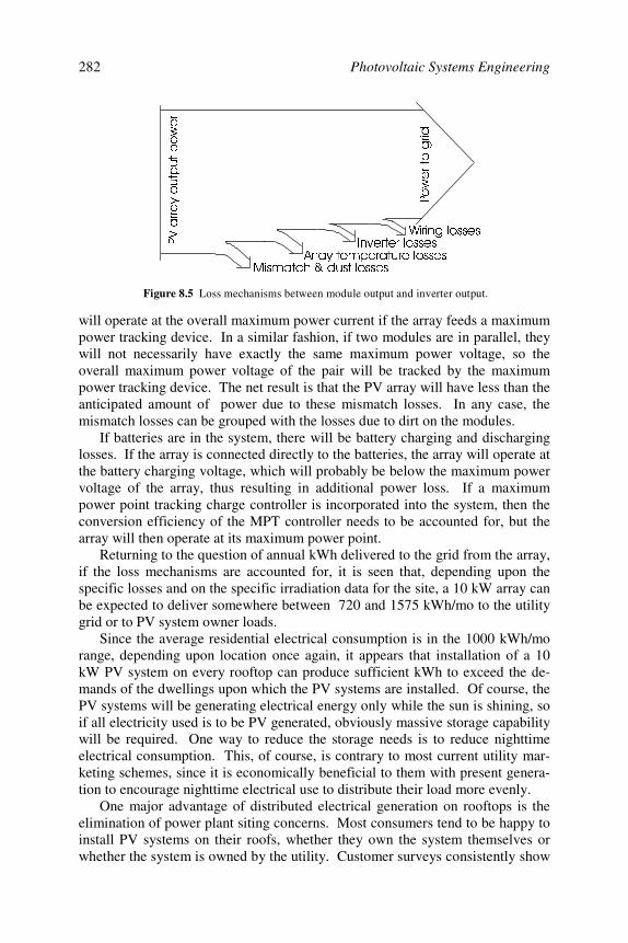
Photovoltaic Systems Engineering282
will operate at the overall maximum power current if the array feeds a maximumpower tracking device. In a similar fashion, if two modules are in parallel, theywill not necessarily have exactly the same maximum power voltage, so theoverall maximum power voltage of the pair will be tracked by the maximumpower tracking device. The net result is that the PV array will have less than theanticipated amount of power due to these mismatch losses. In any case, themismatch losses can be grouped with the losses due to dirt on the modules.
If batteries are in the system, there will be battery charging and discharginglosses. If the array is connected directly to the batteries, the array will operate atthe battery charging voltage, which will probably be below the maximum powervoltage of the array, thus resulting in additional power loss. If a maximumpower point tracking charge controller is incorporated into the system, then theconversion efficiency of the MPT controller needs to be accounted for, but thearray will then operate at its maximum power point.
Returning to the question of annual kWh delivered to the grid from the array,if the loss mechanisms are accounted for, it is seen that, depending upon thespecific losses and on the specific irradiation data for the site, a 10 kW array canbe expected to deliver somewhere between 720 and 1575 kWh/mo to the utilitygrid or to PV system owner loads.
Since the average residential electrical consumption is in the 1000 kWh/morange, depending upon location once again, it appears that installation of a 10kW PV system on every rooftop can produce sufficient kWh to exceed the de-mands of the dwellings upon which the PV systems are installed. Of course, thePV systems will be generating electrical energy only while the sun is shining, soif all electricity used is to be PV generated, obviously massive storage capabilitywill be required. One way to reduce the storage needs is to reduce nighttimeelectrical consumption. This, of course, is contrary to most current utility mar-keting schemes, since it is economically beneficial to them with present genera-tion to encourage nighttime electrical use to distribute their load more evenly.
One major advantage of distributed electrical generation on rooftops is theelimination of power plant siting concerns. Most consumers tend to be happy toinstall PV systems on their roofs, whether they own the system themselves orwhether the system is owned by the utility. Customer surveys consistently show
0LVPDWFKGXVWORVVHV$UUD\WHPSHUDWXUHORVVHV
:LULQJORVVHV,QYHUWHUORVVHV3
9DUUD\RXWSXWSRZHU
3RZHUWRJULG
Figure 8.5 Loss mechanisms between module output and inverter output.
Chapter 8 Utility Interactive PV Systems 283
customer support of cleaner generation, even if it has a premium price. If thechoice becomes that of a PV system on their roof vs. a coal or nuclear plantnearby, the PV system becomes an even more attractive choice for most con-sumers. For those who perceive PV systems as aesthetically unappealing, itmust be remembered that beauty is in the eye of the beholder.
8.4.2 Array Installation
The preferred orientation of a PV array will normally be south facing,mounted in a fixed position, tilted at 90% of latitude. This positioning will usu-ally result in maximum annual kWh generation by the array. Depending uponthe duration of utility peak load and the difference between utility peak load andutility base load, it may be desirable to mount the array with a different expo-sure. Although the alternate mounting may result in generation at preferredutility times, the alternate mounting will generally result in a reduction of annualkWh production. Thus, unless the utility has a preferred rate for peak electricity,it may not be worth it to the system owner to orient the array to coincide withutility peaking. In some cases a compromise can be had, especially when theroof of the dwelling has more west-facing exposure than south-facing exposure.Then some modules can be mounted with each orientation.
Arrays mounted on a roof of a residence require ground fault protection forthe array output. Ground mounted arrays do not require ground fault protection,but may require protection from vandalism. Whether roof mounted or groundmounted, the mount and array assembly must meet mechanical requirements asdiscussed in Chapter 6.
8.4.3 PCU Selection and Mounting
It should be remembered that PCUs are not noise-free. In a manner similarto fluorescent light ballasts and other magnetic loads, the PCUs may produce a120 Hz hum. They should thus be mounted in as practical a location as possiblefrom an electrical and mechanical perspective, but should also not be mountedwhere noise will be an annoyance. Generally, mounting the PCU outdoors or ina garage or carport is acceptable. If it is mounted near an air conditioner com-pressor or a swimming pool pump, the PCU noise will be pretty much maskedby the other noise. Fortunately the PCU is not noisy at night.
When selecting a PCU, it is important to remember to specify a utility inter-active unit, since there are a wide variety of units available. Some are straightutility interactive, some can be used as utility interactive as well as stand-aloneand some are intended for stand-alone use only. While a wide range of per-formance specifications may be available for any unit, it is important to identifythose parameters that are most significant. Features to consider may include anyor all of the following:
IEEE 929 and UL 1741 If the PCU has a UL 1741 listing, then it has beentested to IEEE Standard 929 and consequently complies with NEC requirements.
Photovoltaic Systems Engineering284
For small systems, all voltage and frequency trip points are factory preset andare not field adjustable.
Power rating Maximum PCU output power is normally specified at anambient temperature of 25°C. Surge power rating is less important for a utilityinteractive PCU, since any surges encountered in the load can generally be metby the utility. For a stand-alone PCU, surge capability is more important. Util-ity interactive units with battery backup act as stand-alone units if the utilitydisconnects, so in this case, the surge capacity becomes relevant.
Peak efficiency It is important to note the input voltage over which thestated peak efficiency is obtained. Since the utility interactive PCU always isloaded by the utility connection, if it is designed with maximum power tracking,it will deliver maximum power to the grid over a wide range of PV input powerand will operate close to peak efficiency over most of the maximum powertracking range. Modern PCUs should have peak efficiencies in excess of 90%over most of the operating range.
Maximum power point tracking range Look for the widest possible rangeof input voltages over which the unit is capable of tracking maximum power.
No-load power consumption No-load power consumption should be verylow, although normally the PCU will operate at maximum power output.
Nighttime losses If the unit operates on power supplied by the PV system,then there will be no nighttime losses. If the unit has a stand-alone mode of op-eration, then one can normally expect it to have a “sleep” mode that consumesvery little power if no loads are connected.
Warranty Most quality PCUs carry at least a 5-year warranty. Check whatthe warranty covers.
Code compliance UL 1741 listing indicates compliance with IEEE 929. Itis possible to purchase PCUs that incorporate additional NEC compliance com-ponents, such as ground fault protection, input and output disconnects, fusiblecombiners for multiple string inputs, so strings will not need to be fused in aremote or difficult-to-access location and weatherproof packaging.
Data monitoring Some PCUs provide optional data monitoring capabilityby digitizing system parameters and making them available on an output bus.Some monitoring is available at the PCU and some units provide for remote datalogging via telephone dial-up or other communication means.
8.4.4 Other Installation Considerations
Prior to commencing the installation, since the system will very likely beinspected by both the utility and the local municipality, it is important to firstcomplete all the necessary permitting paperwork. This may offer an excellentopportunity for the engineer to perform an educational public service by an-swering any questions either authority may have about the installation.
Persons not familiar with IEEE 929, UL 1741 and Article 690 of the NECmay be reluctant to accept the straightforward installation allowed by thesecodes and standards. It is possible that the most time-consuming part of the in-
Chapter 8 Utility Interactive PV Systems 285
stallation may be convincing the inspectors that the installation will be safe,competent and code compliant. Fortunately, electrical inspectors tend to be wellversed on the NEC and are generally interested in new technology.
It is also conceivable that a zoning restriction on installation of rooftop solarsystems on the street side of a building may exist. The permitting process maythen involve a trip or two to zoning boards or town council meetings, perhapswith an attorney or a delegation of solar enthusiasts.
8.4.5 A 2.5 kW Residential Rooftop Utility Interactive PV System
PCU SelectionA number of factors may enter the decision-making process associated with
installation of a residential PV system. Perhaps the area of rooftop availablewill be a limiting factor. Perhaps it will be budget. Unlike the decision processfor stand-alone systems, the first item of consideration is not necessarily theload. In this section, a nominal 2.5 kW residential rooftop interactive systemwill be designed. A 2.5 kW system has been selected because an interesting 2.5kW PCU is available and sufficient roof area is also available. The system is tobe installed in a southern location where the maximum array temperature will be60°C and the minimum array temperature will be −10°C.
The particular PCU is listed under UL 1741 and has the following operatingspecifications:
dc Input Input Voltage Range 250−550 VMaximum Input Current 11.2 A
ac Output Voltage 240 V 1 ϕNominal Output Power 2200 WPeak Power 2500 WTotal Harmonic Distortion < 4%Maximum Efficiency 94%
General Internal consumption in operation ≤ 7 WInternal consumption in standby 0.25 WWeight 30 kg
A particularly useful feature of this inverter is the use of the power line fortransmission of data to a computer that can then be used for monitoring pur-poses, thus eliminating wiring for data monitoring except for sensors.
PCU MountingAs luck would have it, the main ac distribution panel is surface mounted,
with adequate space next to it for mounting the PCU. It is located where a littlehum from the PCU will not annoy anyone and where it has an open space for a2-pole circuit breaker. The weight of the PCU must be considered carefully
Photovoltaic Systems Engineering286
when the PCU is mounted and all instructions provided by the manufacturershould be followed.
Module SelectionThe next step is to select an appropriate module for the system input.
Working backward from the PCU input requirements, using NEC requirements,a set of limiting conditions can be established for the module(s). First of all,NEC Table 690.7 requires multiplication of VOC of a Si array by 1.13 to correctfor the −10°C input temperature. Thus, the maximum VOC of the array at 25°Cis limited to 486 V to keep the array output voltage below 550 V over the oper-ating temperature range. The array ISC must be limited so that 1.25 ISC will beless than the PCU rated input current. Thus, ISC ≤ 8.96 A.
Coincidentally, a certain crystalline Si module has the following operatingspecifications:
Pmax 120 WVm 17.1 VIm 7.0 AVOC 21.0 VISC 7.2 Adimensions 26 Bypass diodes internal to the module
Note that if 22 of these modules are connected in series, VOC for the stringwill be 462 V, which lies nicely within the input voltage limitations. At maxi-mum power under standard test conditions, the string voltage will be 376 V,again, nicely within the limits of maximum power tracking. Furthermore, 125%of ISC also lies nicely within the PCU input current limits. Finally, the maxi-mum total array output power will be 2640 W. Although this power level ex-ceeds the 2500 W rating of the inverter, this array power is acceptable, since it isat standard test conditions, and the inverter power rating applies to the inverteroutput power. With a 0.5%/°C decrease in power for array temperatures above25°C, and with a typical array temperature of 55°C, the array output power de-creases to 2244 W. Array mismatch, dust and wiring losses may reduce the ar-ray output power by another 10%, so a more typical inverter input power will becloser to 2020 W, which is well below the inverter output power rating. With aninverter efficiency of 94%, this results in an inverter output power of about 1900W under irradiation of 1 kW/m2.
Module MountingNormally the modules will be mounted securely in a south-facing direction
several inches above and parallel to the roof slope. Several commercial arraymounting kits are available for this purpose. These kits provide sufficient flexi-bility in the location of mounting points to ensure that the array mounts will besecured to roof trusses or to spanners that have been installed between rooftrusses to provide a secure mounting for the array. The commercial kits are en-
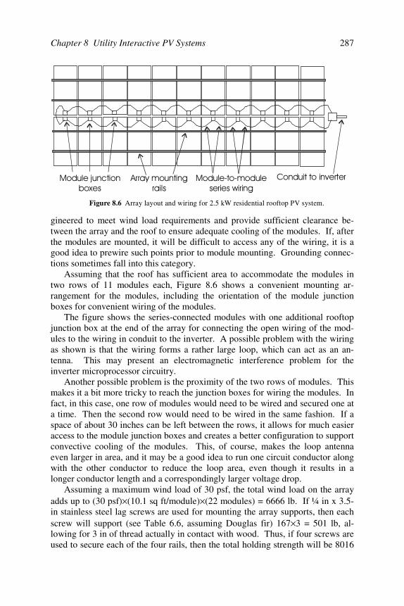
Chapter 8 Utility Interactive PV Systems 287
gineered to meet wind load requirements and provide sufficient clearance be-tween the array and the roof to ensure adequate cooling of the modules. If, afterthe modules are mounted, it will be difficult to access any of the wiring, it is agood idea to prewire such points prior to module mounting. Grounding connec-tions sometimes fall into this category.
Assuming that the roof has sufficient area to accommodate the modules intwo rows of 11 modules each, Figure 8.6 shows a convenient mounting ar-rangement for the modules, including the orientation of the module junctionboxes for convenient wiring of the modules.
The figure shows the series-connected modules with one additional rooftopjunction box at the end of the array for connecting the open wiring of the mod-ules to the wiring in conduit to the inverter. A possible problem with the wiringas shown is that the wiring forms a rather large loop, which can act as an an-tenna. This may present an electromagnetic interference problem for theinverter microprocessor circuitry.
Another possible problem is the proximity of the two rows of modules. Thismakes it a bit more tricky to reach the junction boxes for wiring the modules. Infact, in this case, one row of modules would need to be wired and secured one ata time. Then the second row would need to be wired in the same fashion. If aspace of about 30 inches can be left between the rows, it allows for much easieraccess to the module junction boxes and creates a better configuration to supportconvective cooling of the modules. This, of course, makes the loop antennaeven larger in area, and it may be a good idea to run one circuit conductor alongwith the other conductor to reduce the loop area, even though it results in alonger conductor length and a correspondingly larger voltage drop.
Assuming a maximum wind load of 30 psf, the total wind load on the arrayadds up to (30 psf) × (10.1 sq ft/module) × (22 modules) = 6666 lb. If ¼ in x 3.5-in stainless steel lag screws are used for mounting the array supports, then eachscrew will support (see Table 6.6, assuming Douglas fir) 167 × 3 = 501 lb, al-lowing for 3 in of thread actually in contact with wood. Thus, if four screws areused to secure each of the four rails, then the total holding strength will be 8016
0 1$&
-+#+
0 **# "
Figure 8.6 Array layout and wiring for 2.5 kW residential rooftop PV system.
Photovoltaic Systems Engineering288
lb, providing an overall safety factor of 8016 × 4.5 ÷ 6666 = 5.4 for the holdingstrength. If the array is centered on the roof, this will reduce the wind loading toa minimum and will most likely provide the most aesthetically pleasing appear-ance.
System WiringThe current rating of the module wiring must be at least 1.25 × 1.25 × 7.2 A =
11.23 A. At a temperature of 60°C, the ampacity of a conductor with 90°C ratedinsulation must be derated to 71%, so the module wiring must be rated at aminimum of 15.82 A at 30°C. Thus, #14 wire is adequate, since #14 with 90°Cinsulation is rated at 25 A at 30°C. If the array junction box is mounted 50 ftfrom the PCU, and if an additional 130 ft of open wiring is used between mod-ules and the array junction box, then the equivalent 2-way distance from mod-ules to PCU will be (130 ÷ 2) + 50 = 115 ft. Hence, if #14 copper wire is used,the resistance of the wiring from array to PCU will be 0.706 Ω . At rated arraycurrent, this will produce a voltage drop of 7.0 × 0.706 = 4.94 V, which is ap-proximately 1.3% of the array output voltage. Hence, #14 Cu wire with 90°Cinsulation is adequate from array to PCU.
For the wiring in conduit between the array junction box and the PCU, #14THWN-2 is readily available. However, it is possible that #14 USE-2 will notbe available for the open wiring between modules. Thus, in order to meet theultraviolet resistant requirements of the open wiring, it may be necessary to use#10 USE-2, which will lower the total wiring resistance to 0.1612 + 0.307 =0.3231 Ω , which will result in a voltage drop of 2.26 V, or 0.6%. All wiring ofmodules and output circuit must have insulation rated at 600 V.
The wiring of the modules and the PV output circuit is particularly simple,since the wire is adequate to carry any worst-case short-circuit current. Hence,per NEC, the inclusion of fuses or blocking diodes in the PV source circuit isoptional. Fusing of the circuit should thus be in accordance with module manu-facturer recommendations, which, in this case, would mean a 12 A fuse, whichis the next size above 156% of the module ISC. The modules contain internalbypass diodes, so no external bypass diodes will be needed.
The wiring from PCU to the distribution panel, assuming the point of com-mon coupling will be at the distribution panel, needs to be rated at 125% of themaximum PCU output current, or 13.02 A. Hence, #14 is also adequate tocarry the PCU output current to the distribution panel, provided that the distancefrom PCU to distribution panel is short enough to limit voltage drop to approxi-mately 2%. At 240 V, this allows for a distance of 75 ft. A 2-pole, 15 A circuitbreaker, labeled as the point of utility connection, will be suitable for the con-nection to the distribution panel.
Grounding, Surge Protection and DisconnectsThe PV system will require ground fault protection as well as dc and ac dis-
connects. The PCU is supplied with input surge protection. The negative PVoutput conductor should be grounded at a single point at the PCU to ensure
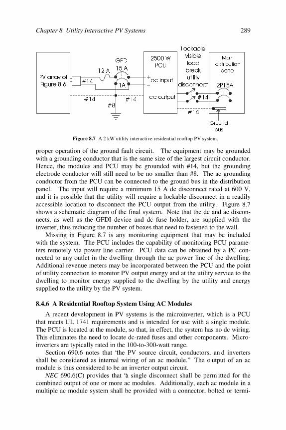
Chapter 8 Utility Interactive PV Systems 289
proper operation of the ground fault circuit. The equipment may be groundedwith a grounding conductor that is the same size of the largest circuit conductor.Hence, the modules and PCU may be grounded with #14, but the groundingelectrode conductor will still need to be no smaller than #8. The ac groundingconductor from the PCU can be connected to the ground bus in the distributionpanel. The input will require a minimum 15 A dc disconnect rated at 600 V,and it is possible that the utility will require a lockable disconnect in a readilyaccessible location to disconnect the PCU output from the utility. Figure 8.7shows a schematic diagram of the final system. Note that the dc and ac discon-nects, as well as the GFDI device and dc fuse holder, are supplied with theinverter, thus reducing the number of boxes that need to fastened to the wall.
Missing in Figure 8.7 is any monitoring equipment that may be includedwith the system. The PCU includes the capability of monitoring PCU parame-ters remotely via power line carrier. PCU data can be obtained by a PC con-nected to any outlet in the dwelling through the ac power line of the dwelling.Additional revenue meters may be incorporated between the PCU and the pointof utility connection to monitor PV output energy and at the utility service to thedwelling to monitor energy supplied to the dwelling by the utility and energysupplied to the utility by the PV system.
8.4.6 A Residential Rooftop System Using AC Modules
A recent development in PV systems is the microinverter, which is a PCUthat meets UL 1741 requirements and is intended for use with a single module.The PCU is located at the module, so that, in effect, the system has no dc wiring.This eliminates the need to locate dc-rated fuses and other components. Micro-inverters are typically rated in the 100-to-300-watt range.
Section 690.6 notes that “the PV source circuit, conductors, an d invertersshall be considered as internal wiring of an ac module.” The o utput of an acmodule is thus considered to be an inverter output circuit.
NEC 690.6(C) provides that “a single disconnect shall be perm itted for thecombined output of one or more ac modules. Additionally, each ac module in amultiple ac module system shall be provided with a connector, bolted or termi-
B
0DLQ
GLVWULEXWLRQ
SDQHO
Figure 8.7 A 2 kW utility interactive residential rooftop PV system.
$
*URXQG
EXV
$
39DUUD\RI
)LJXUH
:
3&8
GFLQSXW
DFRXWSXW
$
*)',
/RFNDEOH
YLVLEOH
ORDG
EUHDN
XWLOLW\
GLVFRQQHFW 3$
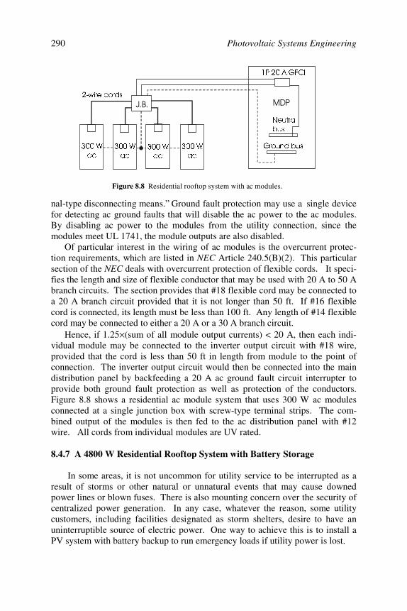
Photovoltaic Systems Engineering290
nal-type disconnecting means.” Ground fault protection may use a single devicefor detecting ac ground faults that will disable the ac power to the ac modules.By disabling ac power to the modules from the utility connection, since themodules meet UL 1741, the module outputs are also disabled.
Of particular interest in the wiring of ac modules is the overcurrent protec-tion requirements, which are listed in NEC Article 240.5(B)(2). This particularsection of the NEC deals with overcurrent protection of flexible cords. It speci-fies the length and size of flexible conductor that may be used with 20 A to 50 Abranch circuits. The section provides that #18 flexible cord may be connected toa 20 A branch circuit provided that it is not longer than 50 ft. If #16 flexiblecord is connected, its length must be less than 100 ft. Any length of #14 flexiblecord may be connected to either a 20 A or a 30 A branch circuit.
Hence, if 1.25 × (sum of all module output currents) < 20 A, then each indi-vidual module may be connected to the inverter output circuit with #18 wire,provided that the cord is less than 50 ft in length from module to the point ofconnection. The inverter output circuit would then be connected into the maindistribution panel by backfeeding a 20 A ac ground fault circuit interrupter toprovide both ground fault protection as well as protection of the conductors.Figure 8.8 shows a residential ac module system that uses 300 W ac modulesconnected at a single junction box with screw-type terminal strips. The com-bined output of the modules is then fed to the ac distribution panel with #12wire. All cords from individual modules are UV rated.
8.4.7 A 4800 W Residential Rooftop System with Battery Storage
In some areas, it is not uncommon for utility service to be interrupted as aresult of storms or other natural or unnatural events that may cause downedpower lines or blown fuses. There is also mounting concern over the security ofcentralized power generation. In any case, whatever the reason, some utilitycustomers, including facilities designated as storm shelters, desire to have anuninterruptible source of electric power. One way to achieve this is to install aPV system with battery backup to run emergency loads if utility power is lost.
2/%/
:DF
:DF
:DF
:DF
3$*)&,
1HXWUDOEXV
*URXQGEXV
03 ZLUHFRUGV
Figure 8.8 Residential rooftop system with ac modules.
Chapter 8 Utility Interactive PV Systems 291
The following system will be designed for residential use with a rooftop-mounted array in order to incorporate a GFDI device in the system, but isequally applicable for installations where the PV array is not on a residentialrooftop. The system source circuits will be run from array junction boxes tosource-circuit combiner boxes located 60 ft from the array junction boxes. Theremaining system components will be located close to the combiner boxes, witha distance of 40 ft between the inverter and the point of utility connection in themain distribution panel. A utility lockable, visible load break disconnect switchwill be located near the utility revenue meter between the inverter and the maindistribution panel. A set of maintenance-free, gel cell lead-acid batteries willalso be located within 6 feet of the inverter.
PCU SelectionAn internet search in early 2003 for utility interactive inverters that are listed
to UL 1741 that can operate in a grid-independent mode upon failure of the util-ity grid results in a small number of units that meet these requirements. Onesuch unit can deliver 5500 W with a nominal 48 V dc input and a 120 V ac out-put. Following are specifications for input, output and general parameters of theunit:
dc Input Input Voltage Range 44-66 VMaximum Input Current 137 A
ac Output Voltage 120 V 1 φRated Output Current 46 AMaximum Surge Current 78 ATotal Harmonic Distortion < 5%Maximum Efficiency 96%
General Internal Consumption in Operation 20 WInternal Consumption in Standby 1 WMaximum Battery Charging Rate 75 A dcWeight 63 kg
The programming of the inverter is extremely flexible, allowing control of awide range of operation modes and system variables, as will be seen as the de-sign progresses. An important feature of the inverter is its battery-charging cir-cuit. When the grid is up and the sun is down, the inverter will charge the bat-teries from the grid if programmed to do so.
Emergency LoadsDetermination of emergency loads for a utility interactive system follows the
same procedure as for a stand-alone system. Any difference lies in the possibil-ity that the PV array may not be able to meet the calculated emergency loadneeds for a prolonged period of grid outage unless adequate PV power is avail-able for charging the batteries when the grid is down. It is possible that space orcost limitations may limit the array power or the battery storage capacity. Since
Photovoltaic Systems Engineering292
numerous calculations of system load have been done in other examples, it willbe assumed for this system that the average daily emergency load is 15kWh/day. This emergency load will be served by an emergency distributionpanel connected to the emergency output terminals of the inverter. Since theemergency loads will have priorities, if it appears that the batteries are dis-charging too much, it will be possible to shut down some of the lights and otherloads designated as emergency loads.
Module selectionThere may also be a wide selection of modules for the PV array, depending
upon whether the roof may impose any geometry constraints. One module thatis attractive for use in this system has the following specifications:
Pmax 150 WVm 17.1 VIm 8.8 AVOC 20.1 VISC 9.2 Adimensions 37.2 Bypass diodes internal to the module
The modules will need to be connected in parallel groups of four in series toproduce the nominal 48 V dc system voltage. If a total of 32 modules are used,then the rated array power will be 4800 watts, produced by eight source circuitsof 4 modules each. It will be assumed that the dwelling has suitable roof ge-ometry to accommodate this array.
An estimate of daily kWh produced by the array can be made if it is assumedthat the batteries are fully charged to a gel cell float voltage of 54.4 V so all PVoutput power is delivered to the inverter. Normally if the array operates at avoltage below Vm, the array current will be somewhat higher than Im. Allowingfor mismatch and dust degradation, it is reasonable to assume the array will op-erate at a current close to 8 × 8.8 = 70.4 A. Multiplying this array current by thebattery float voltage gives 3830 W to the inverter input, which, at 94% inverterand wiring efficiency, will deliver 3600 W to the emergency loads. Any powernot delivered to the emergency loads will be delivered to the balance of thedwelling loads, and then to the utility if all the dwelling loads are satisfied. For5 daily peak sun hours, this means the array can deliver approximately 18kWh/day to the ac loads. This is particularly convenient, since it has alreadybeen established that the emergency loads will be approximately 15 kWh/day.The PV array is thus reasonably closely matched to the emergency loads.
Battery SelectionThe question is, How many days of storage are needed for this system? In
most cases, if there is a utility outage, it will be for a few hours or less. In ex-treme cases, the utility outage may last for a few days. It is anticipated that ifone day of storage is provided, that if utility power is lost for more than a day,
Chapter 8 Utility Interactive PV Systems 293
the PV system will at least partially recharge the batteries each day that the util-ity is down. So in this case, the initial system will be designed with storage forone day, with the possibility of expanding the system if one day of storage isfound to be inadequate.
Converting 15 kWh/day to Ah/day @ 48 V dc results in the need for 312 Ahof storage. Allowing for an 80% depth of discharge, this brings the storage re-quirements up to 390 Ah. Close to this amount of storage can be obtained byusing 180 Ah @ 12 V sealed gel cell lead-acid batteries. Eight batteries will beneeded to provide 360 Ah of storage.
Charge ControlWith an array current of 70.4 A, two 45 A charge controllers (125% of 70.4
A) will be needed. The only time these controllers will be used by the system,will be if the grid is disconnected and if the PV system provides more energythan the emergency loads need. In this case, the controllers will need to shutdown the array to prevent battery overcharge. For the rest of the time, thecharge controllers should be sending all array current to the inverter. This willrequire careful adjustment of the charging limits on the charge controller.
The charge controllers are normally supplied with battery temperature sen-sors for attaching to one of the batteries to monitor battery temperature and pro-vide automatic adjustment of charging settings to compensate for temperature.
Source Circuit Combiner BoxesIn this system, it will be convenient to use two source-circuit combiner
boxes to balance the PV supply between the two charge controllers. Since therewill be a total of eight source circuits, four circuits will be connected to eachcombiner box. Since ISC of each of the source circuits is 9.2 A, and since 156%of 9.2 A is 14.35 A, the source circuits will be fused at 15 A.
Wire SizesModule wiring will be open, using USE-2 insulated wire, with a 28-ft total
round-trip wire length between modules and junction box. Since the distancefrom each source circuit to the source circuit combiner box is 60 ft, and since Im
= 8.8 A for each source circuit, for a 48 V system, to keep the voltage drop insource circuits below 2%, the Ω /kft of the wire must be less than 0.9091. Thiswill require that #8 copper wire be used. If #10 USE-2 wire is used for moduleinterconnection and is then connected to the #8 wire in the rooftop junction box,the total resistance of each source circuit will be 0.12 × 0.764 + 0.028 × 1.21 =0.1256 Ω . The overall %V.D. will thus be 2.3% under full sun conditions,which is acceptable. Use of #8 USE-2 would keep the overall %V.D. < 2%.
The final decision on wire size must also include a check on the ampacity ofthe proposed conductors. If two rooftop junction boxes are incorporated, and ifa single conduit leads from each junction box to the source circuit combiner box,then each conduit will carry four source circuits, or eight current-carrying wires.If the maximum operating temperature of the wiring from junction box to com-
Photovoltaic Systems Engineering294
biner box is 55°C, then the #8 THWN-2 wire ampacity must be derated to 76%of 55 A = 41.8 A (NEC Table 310.16). The eight current-carrying wires in asingle conduit require an additional 70% derating factor (NEC Table310.15(B)(2)(a)), which brings the ampacity down to 29.26 A, which is stillcomfortably higher than the required 156% of ISC. Hence the #8 and even the#10 have adequate ampacities, since the conduit fill derating would not apply tothe #10 intermodule wiring.
It should be noted that although NEC Table 310.17 allows significantlyhigher ampacities for conductors in free air, and although it is tempting to usethese values for the open wiring between modules, it is subject to the ampacitiesof Table 310.16 since the open wiring terminates in junction boxes. Since #8wiring is used for the modules, #8 must be used for the module grounding con-ductors. Hence, each conduit from array junction box to source circuit combinerbox will contain 9 #8 THWN-2 conductors. This means the conduit size mustbe at least 1 !"#$$%!&%"
With four source circuits combined in each source circuit combiner box, thePV output circuit current from each combiner box will be 125% of 4 × ISC, or 46A. The wire must be sized to handle 125% of this current, since the circuit mustbe rated for continuous duty. Thus, the ampacity of the PV output circuits mustbe at least 57.5 A. These circuits are inside at ground level, so no deratings ap-ply and #6 THHN copper is the appropriate wire size.
The rated inverter output circuit current is 46 A, so the wiring from inverteroutput to the point of utility connection must have a minimum ampacity of125% of this value, or 57.5 A. So again, #6 is the appropriate wire size.
Since the maximum inverter input current is 137 A, and since 125% of thiscurrent is 171 A, it is common practice, recommended by the manufacturer, touse 2/0 copper battery cables and a 175 A dc circuit breaker capable of inter-rupting 10,000 A as the battery fuse/disconnect.
The grounding electrode for the dc side of the PV system will be a groundrod. This means that a #6 copper wire is the appropriate grounding electrodeconductor (NEC 250.166(C)). All other equipment grounding conductors can be#10, since the NEC allows #10 grounding conductors between points protectedby 60A overcurrent devices (NEC 250.122)
Fuses, Circuit Breakers, Disconnects, GFDI and Surge Suppression DevicesThe source circuit fuses have already been sized at 15 A. The PV output
conductors from each source-circuit combiner box will first connect to the GFDIdevice, and then to individual 60 A dc circuit breakers between the GFDI deviceand the inverter input. Either the GFDI or the 60 A circuit breakers can serve asthe disconnect for the PV output circuits. The 60 A circuit breakers provideovercurrent protection for the PV output circuits. Surge suppression devices arenormally connected at the inputs to the charge controllers.
The battery disconnect has also been discussed. The load side of this dis-connect is connected directly to the inverter input terminals along with thecharge controller outputs.
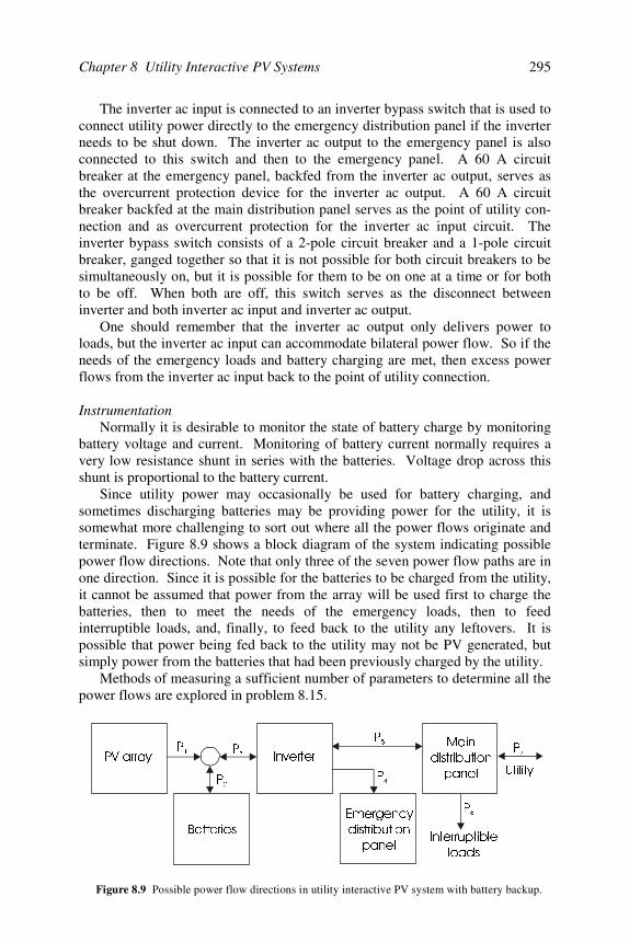
Chapter 8 Utility Interactive PV Systems 295
The inverter ac input is connected to an inverter bypass switch that is used toconnect utility power directly to the emergency distribution panel if the inverterneeds to be shut down. The inverter ac output to the emergency panel is alsoconnected to this switch and then to the emergency panel. A 60 A circuitbreaker at the emergency panel, backfed from the inverter ac output, serves asthe overcurrent protection device for the inverter ac output. A 60 A circuitbreaker backfed at the main distribution panel serves as the point of utility con-nection and as overcurrent protection for the inverter ac input circuit. Theinverter bypass switch consists of a 2-pole circuit breaker and a 1-pole circuitbreaker, ganged together so that it is not possible for both circuit breakers to besimultaneously on, but it is possible for them to be on one at a time or for bothto be off. When both are off, this switch serves as the disconnect betweeninverter and both inverter ac input and inverter ac output.
One should remember that the inverter ac output only delivers power toloads, but the inverter ac input can accommodate bilateral power flow. So if theneeds of the emergency loads and battery charging are met, then excess powerflows from the inverter ac input back to the point of utility connection.
InstrumentationNormally it is desirable to monitor the state of battery charge by monitoring
battery voltage and current. Monitoring of battery current normally requires avery low resistance shunt in series with the batteries. Voltage drop across thisshunt is proportional to the battery current.
Since utility power may occasionally be used for battery charging, andsometimes discharging batteries may be providing power for the utility, it issomewhat more challenging to sort out where all the power flows originate andterminate. Figure 8.9 shows a block diagram of the system indicating possiblepower flow directions. Note that only three of the seven power flow paths are inone direction. Since it is possible for the batteries to be charged from the utility,it cannot be assumed that power from the array will be used first to charge thebatteries, then to meet the needs of the emergency loads, then to feedinterruptible loads, and, finally, to feed back to the utility any leftovers. It ispossible that power being fed back to the utility may not be PV generated, butsimply power from the batteries that had been previously charged by the utility.
Methods of measuring a sufficient number of parameters to determine all thepower flows are explored in problem 8.15.
39DUUD\
%DWWHULHV
,QYHUWHU
(PHUJHQF\
GLVWULEXWLRQ
SDQHO
0DLQ
GLVWULEXWLRQ
SDQHO 8WLOLW\
,QWHUUXSWLEOH
ORDGV
3
3
3
3
3
33
Figure 8.9 Possible power flow directions in utility interactive PV system with battery backup.
Photovoltaic Systems Engineering296
System Commissioning Unlike the previous examples for which the inverters and systems constitute
essentially “plug and play” systems, a system with battery back up will requireon-site programming of the inverter and charge controllers during system start-up to ensure proper system performance.
Normally it will be desirable to have the PV system as the primary batterycharger. To achieve this, the PV charge controller settings must be set to ensurefull battery charge for the type of battery used in the system. Different types ofbatteries require different charge controller settings. The charge control settingson the inverter should be set so the batteries will charge at approximately a C/10rate, and should be set so the batteries will not charge beyond 80%, so the PVsystem will finish the charging process. Alternatively, since the inverter willhave a real-time clock, the inverter can be set to charge the batteries only atnight if the PV system has not fully charged the batteries. Once the batterieshave reached full charge, they will not normally be cycled unless a time of usesell rate is established with the utility. In this case, it may be desirable to sellenergy from the batteries to the utility during utility peak time and rechargethem from the utility during off-peak hours.
The “sell” voltage at the inverter input must then be set so wh en the batteriesare fully charged, the output of the charge controllers will feed the inverter di-rectly for conversion to ac to supply the system loads or sell back to the utility.It is important that the “sell” voltage of the inverter is set low enough to ensurethat the PV charge controllers will think the batteries need charging and willfeed the total PV output current to the inverter input, but not so low that thebatteries will discharge to an unacceptable level to provide “s ell power.”
Complete SystemFigure 8.10 shows the complete system except for instrumentation connec-
tions. As a final note, at the time of this writing, the inverter selected requiresan additional interface with the utility. If the reader plans to use this example asa system design, it will be necessary to check to see whether the additional inter-face is still required or whether a newer model is available from any of theinverter manufacturers.
Note also that the emergency panel will have both busbars connected to-gether so it will be strictly a 120 V distribution panel. The NEC requires that itbe labeled accordingly. Furthermore, the NEC requires that the sum of currentratings of all circuit breakers that supply power to a residential occupancy notexceed 120% of the current ratings of the busbars in the main distribution panel.This means that the 60 A circuit breaker from the PV system, when added towhatever main circuit breaker is connected to the utility supply to the main dis-tribution panel, must not exceed this limit. The PV point of utility connection isshown to be located physically near the bottom of the busbar to minimize thetotal current at any point on the busbar.
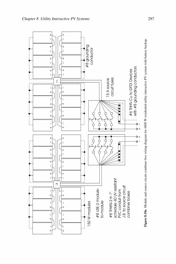
Chapter 8 Utility Interactive PV Systems 297
-%
-%
,45#
678*.# *
*#
6795:*.,;
! <+
#
2/%/
#
$$&
,4-
67
69:=33
"!67
Fig
ure
8.10
a M
odul
e an
d so
urce
cir
cuit
com
bine
r bo
x w
irin
g di
agra
m f
or 4
800
W r
esid
enti
al u
tility
inte
ract
ive
PV
sys
tem
with
bat
tery
bac
k up.
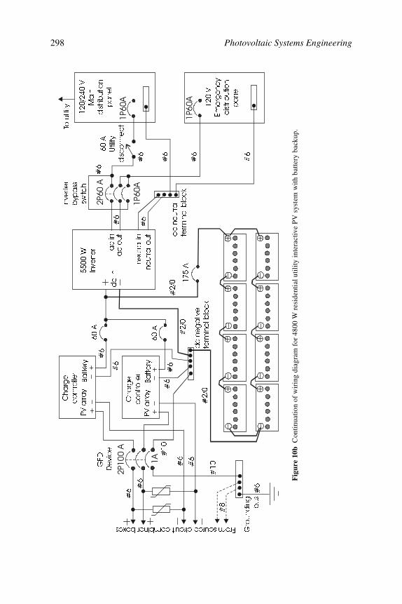
Photovoltaic Systems Engineering298
,-
, -
, -
, -
. ,-
. -
&KDUJH
FRQWUROOHU
&KDUJH
FRQWUROOHU
39DUUD\
39DUUD\
%DWWHU\
%DWWHU\
)URPVRXUFHFLUFXLWFRPELQHUER[HV
*)',
'HYLFH
$
$
$
:
,QYHUWHU
GFLQ
DFLQ
DFRXW
QHXWUDOLQ
QHXWUDORXW
,QYHUWHU
E\SDVV
VZLWFK
9
0DLQ
GLVWULEXWLRQ
SDQHO
7RXWLOLW\
DFQHXWUDO
WHUPLQDOEORFN
GFQHJDWLYH
WHUPLQDOEORFN
*URXQGLQJ
EXV
9
(PHUJHQF\
GLVWULEXWLRQ
SDQHO
$
8WLOLW\
GLVFRQQHFW
Fig
ure
10b
Con
tinua
tion
of w
irin
g di
agra
m f
or 4
800
W r
esid
enti
al u
t ility
inte
ract
ive
PV
sys
tem
with
bat
tery
bac
kup.
Chapter 8 Utility Interactive PV Systems 299
8.5 Medium Utility Interactive PV Systems
8.5.1 Introduction
All the considerations covered in Sections 8.4.1 through 8.4.4 apply to me-dium-sized utility interactive systems. Medium-sized utility interactive PV sys-tems deliver power in the range of 10 kW to 500 kW.
In addition to the considerations for small systems, one must consider thatmedium systems may operate at higher voltages. If the system voltage is over600 volts, then the provisions of NEC Article 490 must be followed. Whilesmall systems must have fixed voltage and frequency setpoints, the utility mayrequire adjustable setpoints on medium systems. In general, the larger the sys-tem, the more likely the system will incorporate custom design requirements tomeet the interconnection requirements of the utility.
The exact size of a medium system will likely be determined by criteriasimilar to the criteria for small systems. In some cases, the available area for thearray may limit the system size. In other cases, available capital may be thelimiting factor. In still other cases, the choice of PCU may be the factor thatdetermines a specific array size. Suitable locations for medium-sized systemsinclude commercial rooftops, church rooftops and other types of institutionalrooftops and parking lot or walkway canopies.
Sometimes medium sized systems are installed as retrofits and in other cases,they are installed as part of the architecture of the building as building-integratedsystems. As thin-film technology continues to progress, it is likely that a widerange of building-integrated PV products will become available. For example,amorphous silicon (a-Si) cells are currently on the market in the form of an inte-grated roofing product. In some cases, not only do integrated PV systems add tothe architectural interest of the structure, they also serve as sunshades for win-dows and as such provide an energy conservation feature as well as an energygeneration feature.
8.5.2 A 16 kW Commercial Rooftop System
One need not drive far to observe that the amount of commercial rooftopspace available for PV system installation appears to be nearly limitless. Com-mercial buildings, particularly in suburban areas, tend to be one-story, flat-roofed, structures, often with more than 10,000 ft2 of roof space. This space isgenerally not shaded, since typically the building will also be surrounded by aparking area. Trees may be planted in a decorative fashion, but will generallynot shade more than a small part of the roof. If the 16 kW system of this exam-ple is constructed with multicrystalline Si modules, the area required will beapproximately 133 m2, or 1435 ft2, assuming 12% efficiency for the modules.For this example, the PV system is owned by the utility and will be connectedon the utility side of the meters.
The building upon which the system is to be installed happens to have a50 ft x 100 ft roof, with the long dimension in a north-south direction. The
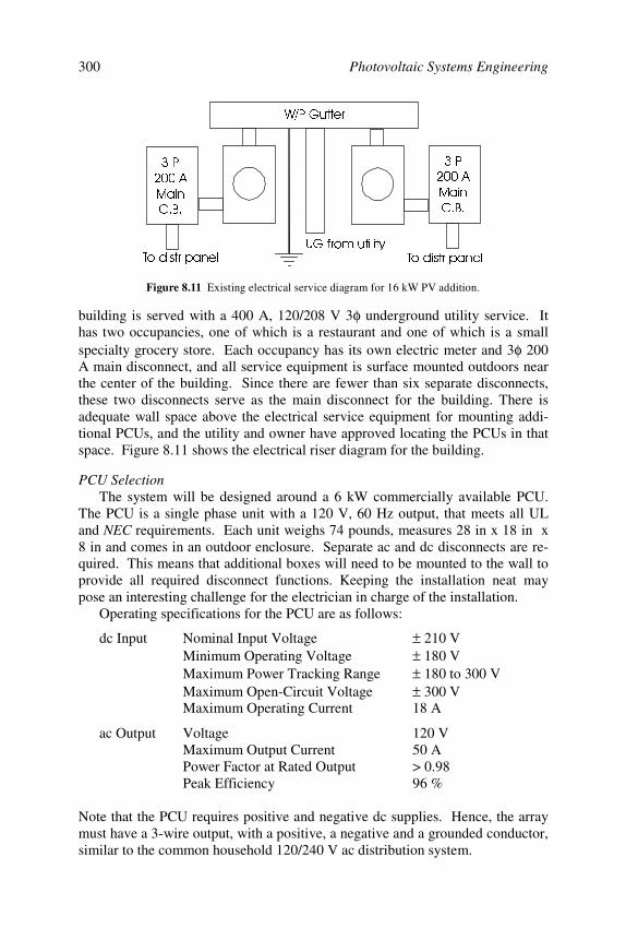
Photovoltaic Systems Engineering300
building is served with a 400 A, 120/208 V 3 φ underground utility service. Ithas two occupancies, one of which is a restaurant and one of which is a smallspecialty grocery store. Each occupancy has its own electric meter and 3 φ 200A main disconnect, and all service equipment is surface mounted outdoors nearthe center of the building. Since there are fewer than six separate disconnects,these two disconnects serve as the main disconnect for the building. There isadequate wall space above the electrical service equipment for mounting addi-tional PCUs, and the utility and owner have approved locating the PCUs in thatspace. Figure 8.11 shows the electrical riser diagram for the building.
PCU SelectionThe system will be designed around a 6 kW commercially available PCU.
The PCU is a single phase unit with a 120 V, 60 Hz output, that meets all ULand NEC requirements. Each unit weighs 74 pounds, measures 28 in x 18 in x8 in and comes in an outdoor enclosure. Separate ac and dc disconnects are re-quired. This means that additional boxes will need to be mounted to the wall toprovide all required disconnect functions. Keeping the installation neat maypose an interesting challenge for the electrician in charge of the installation.
Operating specifications for the PCU are as follows:
dc Input Nominal Input Voltage ± 210 VMinimum Operating Voltage ± 180 VMaximum Power Tracking Range ± 180 to 300 VMaximum Open-Circuit Voltage ± 300 VMaximum Operating Current 18 A
ac Output Voltage 120 VMaximum Output Current 50 APower Factor at Rated Output > 0.98Peak Efficiency 96 %
Note that the PCU requires positive and negative dc supplies. Hence, the arraymust have a 3-wire output, with a positive, a negative and a grounded conductor,similar to the common household 120/240 V ac distribution system.
3
$
0DLQ
&%
3
$
0DLQ
&%
8*IURPXWLOLW\7RGLVWUSDQHO 7RGLVWUSDQHO
:3*XWWHU
Figure 8.11 Existing electrical service diagram for 16 kW PV addition.
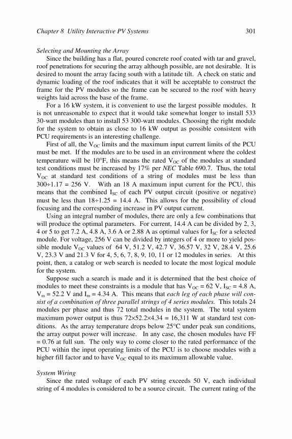
Chapter 8 Utility Interactive PV Systems 301
Selecting and Mounting the ArraySince the building has a flat, poured concrete roof coated with tar and gravel,
roof penetrations for securing the array although possible, are not desirable. It isdesired to mount the array facing south with a latitude tilt. A check on static anddynamic loading of the roof indicates that it will be acceptable to construct theframe for the PV modules so the frame can be secured to the roof with heavyweights laid across the base of the frame.
For a 16 kW system, it is convenient to use the largest possible modules. Itis not unreasonable to expect that it would take somewhat longer to install 53330-watt modules than to install 53 300-watt modules. Choosing the right modulefor the system to obtain as close to 16 kW output as possible consistent withPCU requirements is an interesting challenge.
First of all, the VOC limits and the maximum input current limits of the PCUmust be met. If the modules are to be used in an environment where the coldesttemperature will be 10°F, this means the rated VOC of the modules at standardtest conditions must be increased by 17% per NEC Table 690.7. Thus, the totalVOC at standard test conditions of a string of modules must be less than300 ÷ 1.17 = 256 V. With an 18 A maximum input current for the PCU, thismeans that the combined ISC of each PV output circuit (positive or negative)must be less than 18 ÷ 1.25 = 14.4 A. This allows for the possibility of cloudfocusing and the corresponding increase in PV output current.
Using an integral number of modules, there are only a few combinations thatwill produce the optimal parameters. For current, 14.4 A can be divided by 2, 3,4 or 5 to get 7.2 A, 4.8 A, 3.6 A or 2.88 A as optimal values for ISC for a selectedmodule. For voltage, 256 V can be divided by integers of 4 or more to yield pos-sible module VOC values of 64 V, 51.2 V, 42.7 V, 36.57 V, 32 V, 28.4 V, 25.6V, 23.3 V and 21.3 V for 4, 5, 6, 7, 8, 9, 10, 11 or 12 modules in series. At thispoint, then, a catalog or web search is needed to locate the most logical modulefor the system.
Suppose such a search is made and it is determined that the best choice ofmodules to meet these constraints is a module that has VOC = 62 V, ISC = 4.8 A,Vm = 52.2 V and Im = 4.34 A. This means that each leg of each phase will con-sist of a combination of three parallel strings of 4 series modules. This totals 24modules per phase and thus 72 total modules in the system. The total systemmaximum power output is thus 72 × 52.2 × 4.34 = 16,311 W at standard test con-ditions. As the array temperature drops below 25°C under peak sun conditions,the array output power will increase. In any case, the chosen modules have FF= 0.76 at full sun. The only way to come closer to the rated performance of thePCU within the input operating limits of the PCU is to choose modules with ahigher fill factor and to have VOC equal to its maximum allowable value.
System WiringSince the rated voltage of each PV string exceeds 50 V, each individual
string of 4 modules is considered to be a source circuit. The current rating of the

Photovoltaic Systems Engineering302
wiring of each string must be at least 1.25 × 1.25 × ISC = 7.5 A. Hence, #14 wirefused at 8 A is an appropriate choice.
Separate source-circuit combiner boxes are used for the positive half and thenegative half of the array. The grounded conductors of each array half arejoined in a junction box and the 3-wire array output is then fed to a 2-pole 30 Adisconnect located near the PCU. When the source circuits are combined intothe output circuit, the wire rating needs to be 1.25 × 1.25 × 3 × 4.8 = 22.5 A. Since#12 wire must be fused at no more than 20 A, #10 fused at 30 A is needed foreach PV output circuit conductor.
Since the system voltage, i.e., the voltage between the negative PV outputcircuit conductor and the positive PV output circuit conductor, is less than 600V, 600 V insulation is adequate and the provisions of NEC Article 490 do notapply to this system. Since the PCU already has surge arrestors at its input andoutput, no additional surge protection is necessary. Grounding of the arrayframes is done with the largest circuit conductor, which in this case is #10.Since the array is not on a residential roof, ground fault protection is not re-quired. The building has a lightning protection system, so the array ground canbe connected into the lightning protection system ground bus.
The output circuit of each phase of the PV array is connected to each PCUthrough a 2-pole fused disconnect rated at 30 A, 600 V dc. The disconnectopens the ungrounded conductors of the PV output circuit. The grounded con-ductor is not opened when the disconnect switch is opened.
Connecting the PCU Output to the UtilityThe conductors for connecting the output of the PCU to the utility must be
rated for at least 125% of the PCU rated output current. In this case, the con-ductor rating must be at least 1.25 × 50 A = 62.5 A. This will require #6 Cu con-ductors fused at 70 A.
A convenient way to make this connection is to use a 3-pole 100 A fuseddisconnect, fused at 70 A per phase with dual element (time delay) fuses. Sincethe inverter will meet UL 1741 requirements, if any one phase requires work, orif a PCU requires repair, the fuse to the phase under repair can be removed todisconnect the phase without disconnecting the other two functioning phases.
Another reason why this is a convenient hookup is that the disconnect isreadily obtainable, since it is for ac, and only one box needs to be mounted tothe wall to serve the outputs of all three PCUs. This leads to a somewhat moreaesthetically pleasing appearance for the back of the building. Finally, since thePV system output is to be spliced inside the gutter on the line side of the meters,only three split-bolt connectors will be needed to make the splice, unless one ofthe meters can be double-lugged on the line side. This means the power to thebuilding will be shut down for a shorter time as the connection is made.
The grounding electrode conductor on the dc side will need to be #6 copper,since #6 is the largest circuit conductor. Figure 8.12 shows the wiring of thesystem, except for grounding conductors.
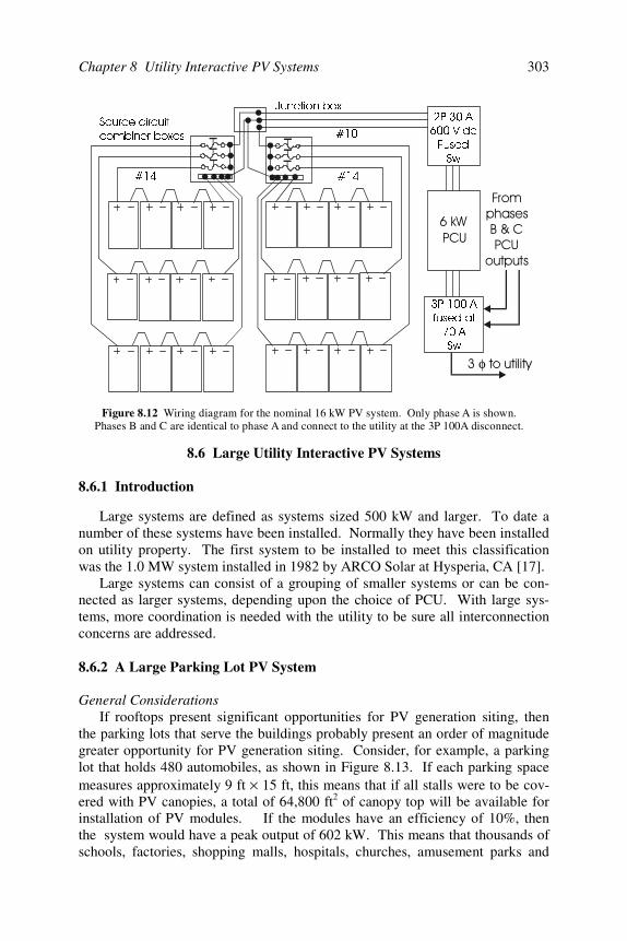
Chapter 8 Utility Interactive PV Systems 303
8.6 Large Utility Interactive PV Systems
8.6.1 Introduction
Large systems are defined as systems sized 500 kW and larger. To date anumber of these systems have been installed. Normally they have been installedon utility property. The first system to be installed to meet this classificationwas the 1.0 MW system installed in 1982 by ARCO Solar at Hysperia, CA [17].
Large systems can consist of a grouping of smaller systems or can be con-nected as larger systems, depending upon the choice of PCU. With large sys-tems, more coordination is needed with the utility to be sure all interconnectionconcerns are addressed.
8.6.2 A Large Parking Lot PV System
General ConsiderationsIf rooftops present significant opportunities for PV generation siting, then
the parking lots that serve the buildings probably present an order of magnitudegreater opportunity for PV generation siting. Consider, for example, a parkinglot that holds 480 automobiles, as shown in Figure 8.13. If each parking spacemeasures approximately 9 ft × 15 ft, this means that if all stalls were to be cov-ered with PV canopies, a total of 64,800 ft2 of canopy top will be available forinstallation of PV modules. If the modules have an efficiency of 10%, thenthe system would have a peak output of 602 kW. This means that thousands ofschools, factories, shopping malls, hospitals, churches, amusement parks and
3$9GF)XVHG6Z
3$IXVHGDW$6Z
=#!+%>
? φ
@5
Figure 8.12 Wiring diagram for the nominal 16 kW PV system. Only phase A is shown.Phases B and C are identical to phase A and connect to the utility at the 3P 100A disconnect.
6RXUFHFLUFXLWFRPELQHUER[HV
-XQFWLRQER[
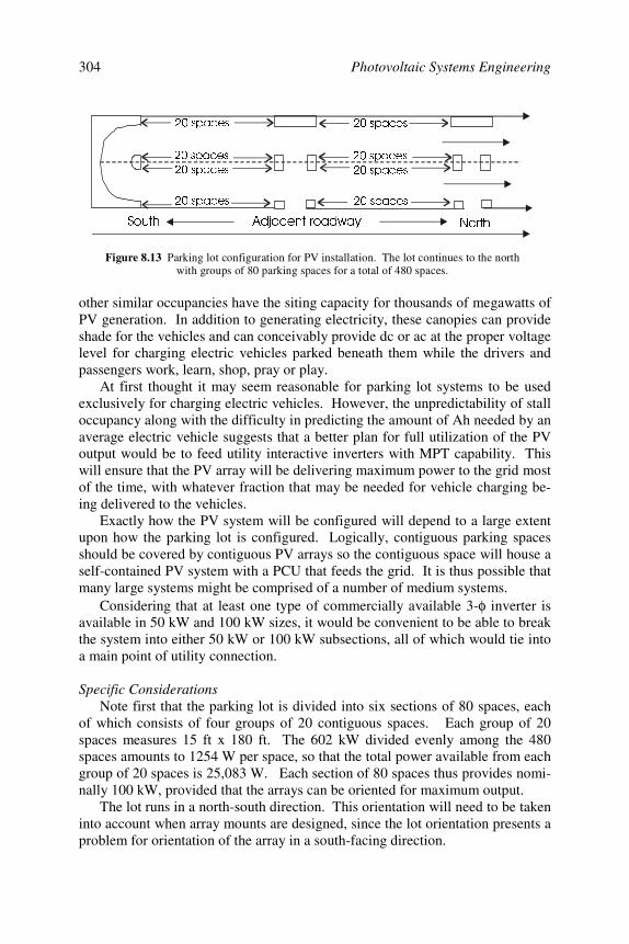
Photovoltaic Systems Engineering304
other similar occupancies have the siting capacity for thousands of megawatts ofPV generation. In addition to generating electricity, these canopies can provideshade for the vehicles and can conceivably provide dc or ac at the proper voltagelevel for charging electric vehicles parked beneath them while the drivers andpassengers work, learn, shop, pray or play.
At first thought it may seem reasonable for parking lot systems to be usedexclusively for charging electric vehicles. However, the unpredictability of stalloccupancy along with the difficulty in predicting the amount of Ah needed by anaverage electric vehicle suggests that a better plan for full utilization of the PVoutput would be to feed utility interactive inverters with MPT capability. Thiswill ensure that the PV array will be delivering maximum power to the grid mostof the time, with whatever fraction that may be needed for vehicle charging be-ing delivered to the vehicles.
Exactly how the PV system will be configured will depend to a large extentupon how the parking lot is configured. Logically, contiguous parking spacesshould be covered by contiguous PV arrays so the contiguous space will house aself-contained PV system with a PCU that feeds the grid. It is thus possible thatmany large systems might be comprised of a number of medium systems.
Considering that at least one type of commercially available 3-φ inverter isavailable in 50 kW and 100 kW sizes, it would be convenient to be able to breakthe system into either 50 kW or 100 kW subsections, all of which would tie intoa main point of utility connection.
Specific ConsiderationsNote first that the parking lot is divided into six sections of 80 spaces, each
of which consists of four groups of 20 contiguous spaces. Each group of 20spaces measures 15 ft x 180 ft. The 602 kW divided evenly among the 480spaces amounts to 1254 W per space, so that the total power available from eachgroup of 20 spaces is 25,083 W. Each section of 80 spaces thus provides nomi-nally 100 kW, provided that the arrays can be oriented for maximum output.
The lot runs in a north-south direction. This orientation will need to be takeninto account when array mounts are designed, since the lot orientation presents aproblem for orientation of the array in a south-facing direction.
VSDFHV
VSDFHV
VSDFHV
VSDFHV
VSDFHV
VSDFHV
VSDFHV
VSDFHV
$GMDFHQWURDGZD\ 1RUWK6RXWK
Figure 8.13 Parking lot configuration for PV installation. The lot continues to the northwith groups of 80 parking spaces for a total of 480 spaces.
Chapter 8 Utility Interactive PV Systems 305
Module Selection and ConfigurationThe next step is to determine a means of configuring a set of modules to
provide the 25,083 W at voltage and current levels consistent with the input re-quirements of the PCU. The 3-phase PCU operating specifications are
dc Input Nominal Input Voltage 325 V dcMinimum Input Voltage 300 V dcMax VOC 600 V dcMax Power Tracking Range 300 to 600 V dcMax Input Current 400 A dcTerminals for combining 6 source circuits
ac Output Voltage (line-to-line) 480 V acMaximum Current 125 A acPower Factor at Rated Output >0.98 .
Naturally, it would be nice if the proposed PV modules fit conveniently into the15 ft x 180 ft space.
Before a module is selected, it should first be noted that the groups of 20parking spaces are in the north-south direction. This complicates the process oftilting the modules at an angle in a south-facing direction, since if the modulesare tilted toward the south, they may partially shade adjacent modules to thenorth. Furthermore, if it rains, the rain will run off the modules directly onto thedrivers and passengers of the vehicles. The modules must therefore be mountedeither horizontally or with a slight tilt toward the east or west. A westward tiltwould be preferred, since it would optimize system output during the afternoonin the summer. The tilt also provides for somewhat better convection cooling ofthe modules and also enables the rain to more effectively clean the modules.Fortunately, the system is located in southern U.S., so a horizontal or slightlywest-facing tilt will not significantly degrade system summer power output.From an aesthetic and structural perspective, however, the canopies over thewest-facing rows, if tilted toward the west, will have the high side at the back ofthe parking space and the low side at the front of the space. If a means of pro-viding adequate support can be found, along with a good argument for contem-porary styling, such a configuration may still be acceptable and need not be dis-carded at this point of the design process.
In the emerging world of module sizes, new sizes often appear on the mar-ket. It is now assumed that after an extensive web search, or, possibly after ne-gotiations with a manufacturer, that a module has been found with VOC = 90V, ISC = 4.4 A, Vmp = 70 V, Imp = 4.0 A, length = 6 ft, width = 5 ft and a tem-perature correction factor for the lowest expected temperature of 10%.
The 10% temperature factor limits the maximum of VOC to 600 ÷ 1.1 = 545 V.Coincidentally, 6 modules in series will have VOC = 540 V. The 15 ft × 180 ftspace can be filled with a total of 90 modules grouped into strings of 6 modules,as shown in Figure 8.14. The 15 groups of 6 modules can be further dividedinto 5 groups of 3 strings of 6, also as noted in Figure 8.14.
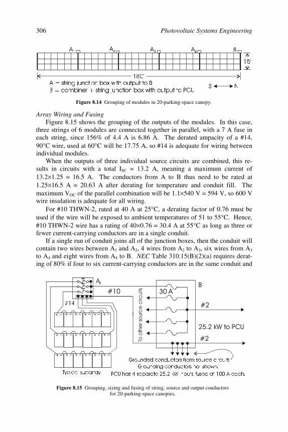
Photovoltaic Systems Engineering306
Array Wiring and FusingFigure 8.15 shows the grouping of the outputs of the modules. In this case,
three strings of 6 modules are connected together in parallel, with a 7 A fuse ineach string, since 156% of 4.4 A is 6.86 A. The derated ampacity of a #14,90°C wire, used at 60°C will be 17.75 A, so #14 is adequate for wiring betweenindividual modules.
When the outputs of three individual source circuits are combined, this re-sults in circuits with a total ISC = 13.2 A, meaning a maximum current of13.2 × 1.25 = 16.5 A. The conductors from A to B thus need to be rated at1.25 × 16.5 A = 20.63 A after derating for temperature and conduit fill. Themaximum VOC of the parallel combination will be 1.1 × 540 V = 594 V, so 600 Vwire insulation is adequate for all wiring.
For #10 THWN-2, rated at 40 A at 25°C, a derating factor of 0.76 must beused if the wire will be exposed to ambient temperatures of 51 to 55°C. Hence,#10 THWN-2 wire has a rating of 40 × 0.76 = 30.4 A at 55°C as long as three orfewer current-carrying conductors are in a single conduit.
If a single run of conduit joins all of the junction boxes, then the conduit willcontain two wires between A1 and A2, 4 wires from A2 to A3, six wires from A3
to A4 and eight wires from A4 to B. NEC Table 310.15(B)(2)(a) requires derat-ing of 80% if four to six current-carrying conductors are in the same conduit and
·
·$ VWULQJMXQFWLRQER[ZLWKRXWSXWWR%
% FRPELQHUVWULQJMXQFWLRQER[ZLWKRXWSXWWR3&8
$
$ $
$ %
16
Figure 8.14 Grouping of modules in 20-parking-space canopy.
7\SLFDOVXEDUUD\
*URXQGHGFRQGXFWRUVIURPVRXUFHFLUFXLWV
3&8KDVVHSDUDWHN:LQSXWVIXVHGDW$HDFK
*URXQGLQJFRQGXFWRUVQRWVKRZQ
L
Figure 8.15 Grouping, sizing and fusing of string, source and output conductorsfor 20-parking-space canopies.
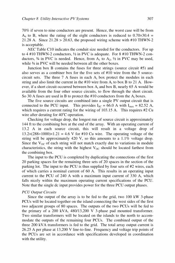
Chapter 8 Utility Interactive PV Systems 307
70% if seven to nine conductors are present. Hence, the worst case will be fromA4 to B, where the rating of the eight conductors is reduced to 0.70 × 30.4 =21.28 A. Since 21.28 > 20.63, the proposed wiring scheme with #10 THWN-2is acceptable.
NEC Table C10 indicates the conduit size needed for the conductors. For upto 4 #10 THWN-2 conductors, ½ in PVC is adequate. For 8 #10 THWN-2 con-ductors, ¾ in PVC is needed. Hence, from A1 to A2, ½ in PVC may be used,while ¾ in PVC will be needed between all the other boxes.
Junction box B contains the fuses for three strings (source circuit #5) andalso serves as a combiner box for the five sets of #10 wire from the 5 source-circuit sets. The three 7 A fuses in each Ai box protect the modules in eachstring and also limit the current in the #10 wire from Ai to box B to 21 A. How-ever, if a short circuit occurred between box Ai and box B, nearly 65 A would beavailable from the four other source circuits, to flow through the short circuit.So 30 A fuses are used in B to protect the #10 conductors from the Ai boxes.
The five source circuits are combined into a single PV output circuit that isconnected to the PCU input. This provides ISC = 66.0 A with Imax = 82.52 A,which requires a current rating for the wiring of 103.15 A. This requires #2 Cuwire after derating for 40oC operation.
Checking for voltage drop, the longest run of source circuit is approximately144 ft to the combining box at the end of the array. With an operating current of13.2 A in each source circuit, this will result in a voltage drop of13.2 × (288 ÷ 1000)× 1.21 = 4.6 V for #10 Cu wire. The operating voltage of thestring will be approximately 420 V, so this amounts to a 1.1% voltage drop.Since the VOC of each string will not match exactly due to variations in modulecharacteristics, the string with the highest VOC should be located farthest fromthe combining box.
The input to the PCU is completed by duplicating the connections of the first20 parking spaces for the remaining three sets of 20 spaces in the section of theparking lot. The input to the PCU is thus supplied by four sets of #2 wires, eachof which carries a nominal current of 60 A. This results in an operating inputcurrent to the PCU of 240 A with a maximum input current of 330 A, whichfalls nicely within the maximum operating current specifications of the PCU.Note that the single dc input provides power for the three PCU output phases.
PCU Output CircuitsSince the output of the array is to be fed to the grid, two 100 kW 3-phase
PCUs will be located together on the island connecting the west sides of the firsttwo adjacent groups of 80 spaces. The outputs of the two PCUs will be fed tothe primary of a 200 kVA, 480/13,200 V 3-phase pad mounted transformer.Two similar transformers will be located on the islands to the north to accom-modate the outputs of the remaining four PCUs. The combined output of thethree 200 kVA transformers is fed to the grid. The total array output current is26.25 A per phase at 13,200 V line-to-line. Frequency and voltage trip points ofthe PCUs are set in accordance with specifications developed in coordinationwith the utility.
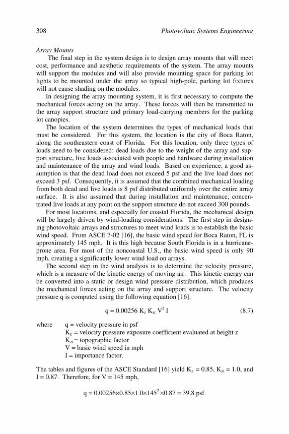
Photovoltaic Systems Engineering308
Array Mounts The final step in the system design is to design array mounts that will meet
cost, performance and aesthetic requirements of the system. The array mountswill support the modules and will also provide mounting space for parking lotlights to be mounted under the array so typical high-pole, parking lot fixtureswill not cause shading on the modules.
In designing the array mounting system, it is first necessary to compute themechanical forces acting on the array. These forces will then be transmitted tothe array support structure and primary load-carrying members for the parkinglot canopies.
The location of the system determines the types of mechanical loads thatmust be considered. For this system, the location is the city of Boca Raton,along the southeastern coast of Florida. For this location, only three types ofloads need to be considered: dead loads due to the weight of the array and sup-port structure, live loads associated with people and hardware during installationand maintenance of the array and wind loads. Based on experience, a good as-sumption is that the dead load does not exceed 5 psf and the live load does notexceed 3 psf. Consequently, it is assumed that the combined mechanical loadingfrom both dead and live loads is 8 psf distributed uniformly over the entire arraysurface. It is also assumed that during installation and maintenance, concen-trated live loads at any point on the support structure do not exceed 300 pounds.
For most locations, and especially for coastal Florida, the mechanical designwill be largely driven by wind-loading considerations. The first step in design-ing photovoltaic arrays and structures to meet wind loads is to establish the basicwind speed. From ASCE 7-02 [16], the basic wind speed for Boca Raton, FL isapproximately 145 mph. It is this high because South Florida is in a hurricane-prone area. For most of the noncoastal U.S., the basic wind speed is only 90mph, creating a significantly lower wind load on arrays.
The second step in the wind analysis is to determine the velocity pressure,which is a measure of the kinetic energy of moving air. This kinetic energy canbe converted into a static or design wind pressure distribution, which producesthe mechanical forces acting on the array and support structure. The velocitypressure q is computed using the following equation [16].
q = 0.00256 Kz Kzt V2 I (8.7)
where q = velocity pressure in psfKz = velocity pressure exposure coefficient evaluated at height zKzt = topographic factorV = basic wind speed in mphI = importance factor.
The tables and figures of the ASCE Standard [16] yield Kz = 0.85, Kzt = 1.0, andI = 0.87. Therefore, for V = 145 mph,
q = 0.00256 × 0.85 × 1.0× 1452 × 0.87 = 39.8 psf.
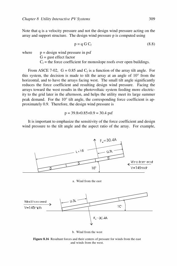
Chapter 8 Utility Interactive PV Systems 309
Note that q is a velocity pressure and not the design wind pressure acting on thearray and support structure. The design wind pressure p is computed using
p = q G Cf (8.8)
where p = design wind pressure in psfG = gust effect factorCf = the force coefficient for monoslope roofs over open buildings.
From ASCE 7-02, G = 0.85 and Cf is a function of the array tilt angle. Forthis system, the decision is made to tilt the array at an angle of 10° from thehorizontal, and to have the arrays facing west. The small tilt angle significantlyreduces the force coefficient and resulting design wind pressure. Facing thearrays toward the west results in the photovoltaic system feeding more electric-ity to the grid later in the afternoon, and helps the utility meet its large summerpeak demand. For the 10° tilt angle, the corresponding force coefficient is ap-proximately 0.9. Therefore, the design wind pressure is
p = 39.8 × 0.85 × 0.9 = 30.4 psf
It is important to emphasize the sensitivity of the force coefficient and designwind pressure to the tilt angle and the aspect ratio of the array. For example,
:LQGIURPHDVW
9 PSK
/ ·
Z
·
·
·
/
R
/
) $Z
:LQGIURPZHVW
9 PSK R
a. Wind from the east
b. Wind from the west
Figure 8.16 Resultant forces and their centers of pressure for winds from the eastand winds from the west.
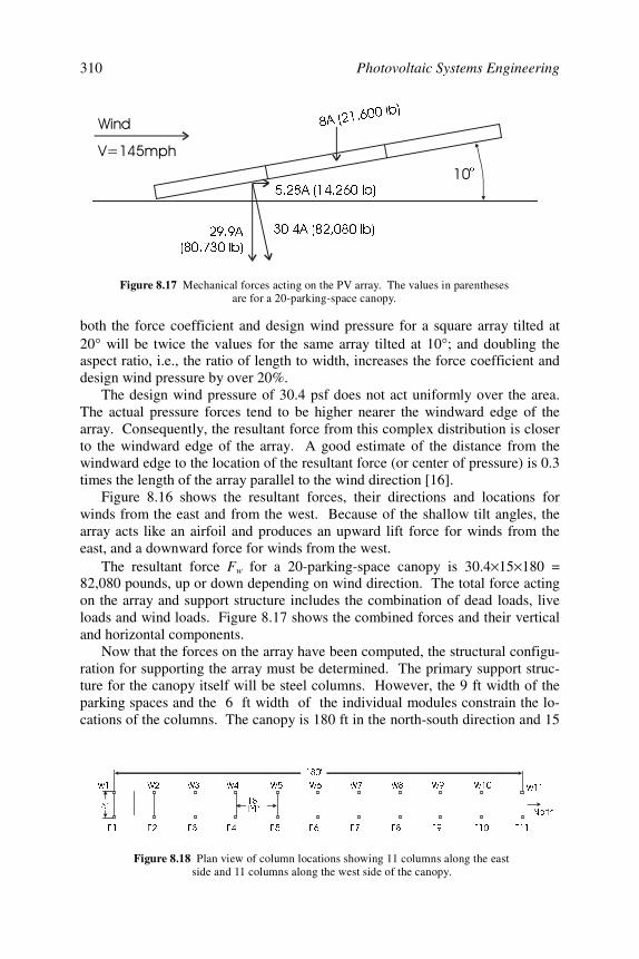
Photovoltaic Systems Engineering310
both the force coefficient and design wind pressure for a square array tilted at20° will be twice the values for the same array tilted at 10°; and doubling theaspect ratio, i.e., the ratio of length to width, increases the force coefficient anddesign wind pressure by over 20%.
The design wind pressure of 30.4 psf does not act uniformly over the area.The actual pressure forces tend to be higher nearer the windward edge of thearray. Consequently, the resultant force from this complex distribution is closerto the windward edge of the array. A good estimate of the distance from thewindward edge to the location of the resultant force (or center of pressure) is 0.3times the length of the array parallel to the wind direction [16].
Figure 8.16 shows the resultant forces, their directions and locations forwinds from the east and from the west. Because of the shallow tilt angles, thearray acts like an airfoil and produces an upward lift force for winds from theeast, and a downward force for winds from the west.
The resultant force Fw for a 20-parking-space canopy is 30.4 × 15 × 180 =82,080 pounds, up or down depending on wind direction. The total force actingon the array and support structure includes the combination of dead loads, liveloads and wind loads. Figure 8.17 shows the combined forces and their verticaland horizontal components.
Now that the forces on the array have been computed, the structural configu-ration for supporting the array must be determined. The primary support struc-ture for the canopy itself will be steel columns. However, the 9 ft width of theparking spaces and the 6 ft width of the individual modules constrain the lo-cations of the columns. The canopy is 180 ft in the north-south direction and 15
$OE
$OE
$
OE
$OER
Figure 8.17 Mechanical forces acting on the PV array. The values in parenthesesare for a 20-parking-space canopy.
1RUWK
:
(((((((((((
::::::::::
·7<3
·
·
Figure 8.18 Plan view of column locations showing 11 columns along the eastside and 11 columns along the west side of the canopy.
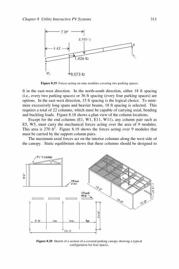
Chapter 8 Utility Interactive PV Systems 311
ft in the east-west direction. In the north-south direction, either 18 ft spacing(i.e., every two parking spaces) or 36 ft spacing (every four parking spaces) areoptions. In the east-west direction, 15 ft spacing is the logical choice. To mini-mize excessively long spans and heavier beams, 18 ft spacing is selected. Thisrequires a total of 22 columns, which must be capable of carrying axial, bendingand buckling loads. Figure 8.18 shows a plan view of the column locations.
Except for the end columns (E1, W1, E11, W11), any column pair such asE5, W5, must carry the mechanical forces acting over the area of 9 modules.This area is 270 ft2. Figure 8.19 shows the forces acting over 9 modules thatmust be carried by the support column pairs.
The maximum axial forces act on the interior columns along the west side ofthe canopy. Static equilibrium shows that these columns should be designed to
OE
!
·
·
(Y
(
:Y
Figure 8.19 Forces acting on nine modules covering two parking spaces.
:KHHOVWRS
·µ
39PRGXOHV
:KHHOVWRS
W\S W\SW\S·µ
·µ
·µ
·µ
·µ
·µ
·µ
Figure 8.20 Sketch of a section of a covered parking canopy showing a typicalconfiguration for four spaces.
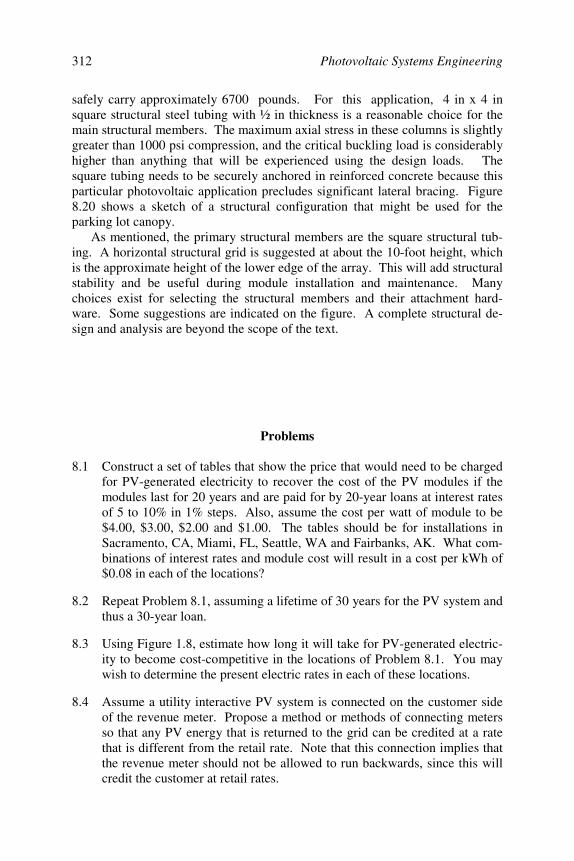
Photovoltaic Systems Engineering312
safely carry approximately 6700 pounds. For this application, 4 in x 4 insquare structural steel tubing with ½ in thickness is a reasonable choice for themain structural members. The maximum axial stress in these columns is slightlygreater than 1000 psi compression, and the critical buckling load is considerablyhigher than anything that will be experienced using the design loads. Thesquare tubing needs to be securely anchored in reinforced concrete because thisparticular photovoltaic application precludes significant lateral bracing. Figure8.20 shows a sketch of a structural configuration that might be used for theparking lot canopy.
As mentioned, the primary structural members are the square structural tub-ing. A horizontal structural grid is suggested at about the 10-foot height, whichis the approximate height of the lower edge of the array. This will add structuralstability and be useful during module installation and maintenance. Manychoices exist for selecting the structural members and their attachment hard-ware. Some suggestions are indicated on the figure. A complete structural de-sign and analysis are beyond the scope of the text.
Problems
8.1 Construct a set of tables that show the price that would need to be chargedfor PV-generated electricity to recover the cost of the PV modules if themodules last for 20 years and are paid for by 20-year loans at interest ratesof 5 to 10% in 1% steps. Also, assume the cost per watt of module to be$4.00, $3.00, $2.00 and $1.00. The tables should be for installations inSacramento, CA, Miami, FL, Seattle, WA and Fairbanks, AK. What com-binations of interest rates and module cost will result in a cost per kWh of$0.08 in each of the locations?
8.2 Repeat Problem 8.1, assuming a lifetime of 30 years for the PV system andthus a 30-year loan.
8.3 Using Figure 1.8, estimate how long it will take for PV-generated electric-ity to become cost-competitive in the locations of Problem 8.1. You maywish to determine the present electric rates in each of these locations.
8.4 Assume a utility interactive PV system is connected on the customer sideof the revenue meter. Propose a method or methods of connecting metersso that any PV energy that is returned to the grid can be credited at a ratethat is different from the retail rate. Note that this connection implies thatthe revenue meter should not be allowed to run backwards, since this willcredit the customer at retail rates.
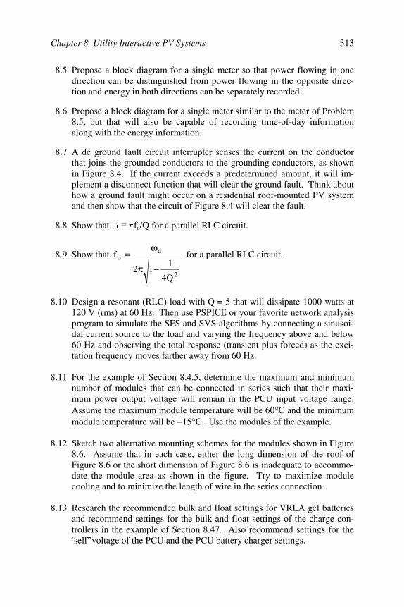
Chapter 8 Utility Interactive PV Systems 313
8.5 Propose a block diagram for a single meter so that power flowing in onedirection can be distinguished from power flowing in the opposite direc-tion and energy in both directions can be separately recorded.
8.6 Propose a block diagram for a single meter similar to the meter of Problem8.5, but that will also be capable of recording time-of-day informationalong with the energy information.
8.7 A dc ground fault circuit interrupter senses the current on the conductorthat joins the grounded conductors to the grounding conductors, as shownin Figure 8.4. If the current exceeds a predetermined amount, it will im-plement a disconnect function that will clear the ground fault. Think abouthow a ground fault might occur on a residential roof-mounted PV systemand then show that the circuit of Figure 8.4 will clear the fault.
8.8 Show o/Q for a parallel RLC circuit.
8.9 Show that
2
do
Q4
112
f
−π
ω= for a parallel RLC circuit.
8.10 Design a resonant (RLC) load with Q = 5 that will dissipate 1000 watts at120 V (rms) at 60 Hz. Then use PSPICE or your favorite network analysisprogram to simulate the SFS and SVS algorithms by connecting a sinusoi-dal current source to the load and varying the frequency above and below60 Hz and observing the total response (transient plus forced) as the exci-tation frequency moves farther away from 60 Hz.
8.11 For the example of Section 8.4.5, determine the maximum and minimumnumber of modules that can be connected in series such that their maxi-mum power output voltage will remain in the PCU input voltage range.Assume the maximum module temperature will be 60°C and the minimummodule temperature will be −15°C. Use the modules of the example.
8.12 Sketch two alternative mounting schemes for the modules shown in Figure8.6. Assume that in each case, either the long dimension of the roof ofFigure 8.6 or the short dimension of Figure 8.6 is inadequate to accommo-date the module area as shown in the figure. Try to maximize modulecooling and to minimize the length of wire in the series connection.
8.13 Research the recommended bulk and float settings for VRLA gel batteriesand recommend settings for the bulk and float settings of the charge con-trollers in the example of Section 8.47. Also recommend settings for the“sell” voltage of the PCU and the PCU battery charger settings.
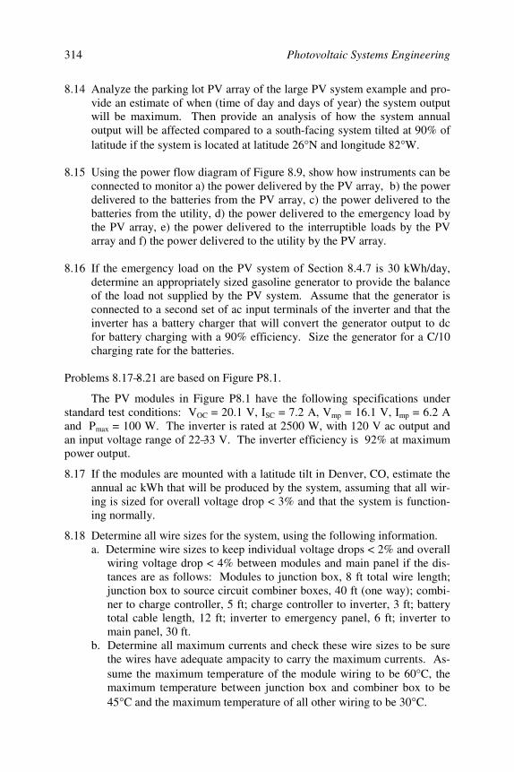
Photovoltaic Systems Engineering314
8.14 Analyze the parking lot PV array of the large PV system example and pro-vide an estimate of when (time of day and days of year) the system outputwill be maximum. Then provide an analysis of how the system annualoutput will be affected compared to a south-facing system tilted at 90% oflatitude if the system is located at latitude 26°N and longitude 82°W.
8.15 Using the power flow diagram of Figure 8.9, show how instruments can beconnected to monitor a) the power delivered by the PV array, b) the powerdelivered to the batteries from the PV array, c) the power delivered to thebatteries from the utility, d) the power delivered to the emergency load bythe PV array, e) the power delivered to the interruptible loads by the PVarray and f) the power delivered to the utility by the PV array.
8.16 If the emergency load on the PV system of Section 8.4.7 is 30 kWh/day,determine an appropriately sized gasoline generator to provide the balanceof the load not supplied by the PV system. Assume that the generator isconnected to a second set of ac input terminals of the inverter and that theinverter has a battery charger that will convert the generator output to dcfor battery charging with a 90% efficiency. Size the generator for a C/10charging rate for the batteries.
Problems 8.17–8.21 are based on Figure P8.1.
The PV modules in Figure P8.1 have the following specifications understandard test conditions: VOC = 20.1 V, ISC = 7.2 A, Vmp = 16.1 V, Imp = 6.2 Aand Pmax = 100 W. The inverter is rated at 2500 W, with 120 V ac output andan input voltage range of 22–33 V. The inverter efficiency is 92% at maximumpower output.
8.17 If the modules are mounted with a latitude tilt in Denver, CO, estimate theannual ac kWh that will be produced by the system, assuming that all wir-ing is sized for overall voltage drop < 3% and that the system is function-ing normally.
8.18 Determine all wire sizes for the system, using the following information.a. Determine wire sizes to keep individual voltage drops < 2% and overall
wiring voltage drop < 4% between modules and main panel if the dis-tances are as follows: Modules to junction box, 8 ft total wire length;junction box to source circuit combiner boxes, 40 ft (one way); combi-ner to charge controller, 5 ft; charge controller to inverter, 3 ft; batterytotal cable length, 12 ft; inverter to emergency panel, 6 ft; inverter tomain panel, 30 ft.
b. Determine all maximum currents and check these wire sizes to be surethe wires have adequate ampacity to carry the maximum currents. As-sume the maximum temperature of the module wiring to be 60°C, themaximum temperature between junction box and combiner box to be45°C and the maximum temperature of all other wiring to be 30°C.
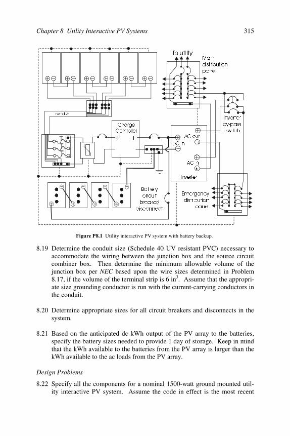
Chapter 8 Utility Interactive PV Systems 315
8.19 Determine the conduit size (Schedule 40 UV resistant PVC) necessary toaccommodate the wiring between the junction box and the source circuitcombiner box. Then determine the minimum allowable volume of thejunction box per NEC based upon the wire sizes determined in Problem8.17, if the volume of the terminal strip is 6 in3. Assume that the appropri-ate size grounding conductor is run with the current-carrying conductors inthe conduit.
8.20 Determine appropriate sizes for all circuit breakers and disconnects in thesystem.
8.21 Based on the anticipated dc kWh output of the PV array to the batteries,specify the battery sizes needed to provide 1 day of storage. Keep in mindthat the kWh available to the batteries from the PV array is larger than thekWh available to the ac loads from the PV array.
Design Problems
8.22 Specify all the components for a nominal 1500-watt ground mounted util-ity interactive PV system. Assume the code in effect is the most recent
Figure P8.1 Utility interactive PV system with battery backup.
BB
&KDUJH&RQWUROOHU
1
1
$&LQ
$&RXW
'&LQ
,QYHUWHU
7RXWLOLW\0DLQ
GLVWULEXWLRQ
SDQHO
(PHUJHQF\
GLVWULEXWLRQ
SDQHO
%DWWHU\
FLUFXLW
EUHDNHU
GLVFRQQHFW
,QYHUWHU
E\SDVV
VZLWFK
FRQGXLW
Photovoltaic Systems Engineering316
version of the NEC. Use a utility connection point on the utility side of themeter.
8.23 Specify all the components and show the design for a nominal 5000-wattresidential rooftop-mounted, utility interactive PV system, based on themost recent version of the NEC. Connect the system on the customer sideof the meter.
8.24 Design a 9.6 kW, customer-owned, commercial rooftop utility interactivePV system with a 120/240 V output and 30 kWh of battery backup. Spec-ify all components and connections.
8.25 Design a 36 kW commercial roof-mounted PV system that will feed a120/208 V 3 φ 400 A distribution panel on the customer side of the meter.Comment on the bus capacity of the distribution panel and the allowablesize of the main circuit breaker on the distribution panel feeder circuit.
8.26 A 120 kW utility interactive system is to be installed as a parking lot can-opy. It is to feed the grid with a 3-phase, 277/480 V balanced output.Draw a system diagram, showing all necessary components, including wiresizes and fuse/circuit breaker sizes and locations. Comment on yourchoice of whether to use a single set of inverters or multiple sets.
References
[1] Osborn, D. E. and Collier, D. E., “Utility Business Opport unities with the Commer-cialization of Grid-Connected PV,” Interconnecting Small PV Sy stems to Florida’sUtility Grid, A Workshop for Florida Utilities, Cocoa, FL, October 22, 1998.
[2] http://SMUD.com for more information on SMUD PV projects. [3] http://www.austinenergy.com/solar-explorer/index.html for information on Austin
Energy renewable energy programs. [4] http://www.bpu.state.nj.us/wwwroot/energy/rfp for information on New Jersey Re-
newable Energy Technology Projects solicitation. [5] Wills, R. H., The Interconnection of Photovoltaic Power Systems with the Utility
Grid: An Overview for Utility Engineers, Sandia National Laboratories, Albuquer-que, NM, 1998.
[6] Maycock, P., The world PV market—production increases 36%, Renewable EnergyWorld, Vol 5, No 4, July-Aug 2002, 146-161.
[7] NFPA 70 National Electrical Code, 2002 Edition, National Fire Protection Associa-tion, Quincy, MA, 2002.
[8] U.S. Senate. 95th Congress, 1st Session. Public Utility Regulatory Policy Act of1977, Washington, D.C., Government Printing Office, 1977.
[9] IEEE 929-2000, “IEEE Recommended Practice for Utility Inte rface of Residentialand Intermediate Photovoltaic (PV) Systems,” IEEE Standards Co ordinating Com-mittee 21, Photovoltaics, 2000.

Chapter 8 Utility Interactive PV Systems 317
[10] UL Subject 1741, “Standard for Power Conditioning Units for use in ResidentialPhotovoltaic Power Systems,” Underwriters Laboratories Inc., 1 997.
[11] ANSI C84.1-1995, Electric Power Systems and Equipment - Voltage Ratings (60Hertz), American National Standards Institute, New York, 1995.
[12] Kern, G. A., Bonn, R. H., Ginn, J., and Gonzalez, S., Results of Sandia NationalLaboratories grid-tied inverter testing, Proc. 2nd World Conf and Exhibition on PVSolar Energy Conversion, Vienna, Austria, July 1998.
[13] Kern, G. A., “New Techniques for Islanding Protection,” In terconnecting Small PVSystems to Florida’s Utility Grid, A Workshop for Florida Utili ties, Cocoa, FL, Oc-tober 22, 1998.
[14] Wiles, J., Photovoltaic Power Systems and the National Electrical Code: SuggestedPractices, SAND2001-0674, Sandia National Laboratories, Albuquerque, NM,March 2001.
[15] CFR 47, Federal Communications Commission, Rules and Regulations, Radio Fre-quency Devices, Part 15, 1994.
[16] SEI/ASCE 7-02, Minimum Design Loads for Buildings and Other Structures,American Society of Civil Engineers, Reston, VA, Jan, 2003.
[17] Forrester, D. L., Qualification testing for a central station, Conference Records of17th IEEE PV Specialists Conference, 1019–1024, Kissimmee, FL, May 1 −4, 1984.
Suggested Reading
NESC–ANSI/NFPA C2-1993, National Electrical Safety Code, National Fire Pro-tection Association, Quincy, MA, 1993.

319
Chapter 9EXTERNALITIES AND PHOTOVOLTAICS
9.1 Introduction
Pollution is an insidious byproduct of civilization that threatens the qualityand integrity of our air, our soils, our water and our infrastructure. The planethas a remarkable ability to cleanse itself, with significant feedback loops inplace for restoration of equilibrium. One example is photosynthesis, in whichthe oxygen–carbon dioxide cycle is sustained by regeneration of oxygen fromthe carbon dioxide of respiration and oxidation. Another is digestion, in whichbacteria process organic matter into a form that enables the matter to enrich soilsor to nourish living bodies.
In electrical engineering terms, the feedback processes can be characterizedin control terms by observing the locations of the poles of the processes. If thepoles are in the left half plane, then the process is stable. If the poles are in theright half plane, then the process is unstable. Stable implies that the process willtend to correct itself. Unstable implies unbounded increase.
While many processes appear to be stable, examples of unstable processeshave also been noted. In particular, increased CO2 from nonpolar regions causeswarming in the polar regions, resulting in thawing of permafrost regions, inwhich large quantities of CH4, another greenhouse gas, are trapped. Liberationof the CH4 causes additional warming, resulting in additional liberation of CH4,and so forth. The question is whether another natural process exists to counter-act this cycle. The process itself is unstable.
Human intervention is at a point where serious questions are now beingasked with regard to the effects of human-generated pollutants in terms of thestability of the solutions of the process equations. One might argue that as longas the poles are kept in the left half plane, the pollution causing the appearanceof the poles is at acceptable levels for the planet to sustain life. The challengebecomes one of defining acceptable limits on pollution and the resulting changesin natural cycles caused by human intervention.
9.2 Externalities
Externalities were mentioned briefly in Section 5.4 as factors resulting fromenergy or other manufacturing that are not incorporated directly into the sellingprice of a product. That is, once the smoke is out of the smokestack, it is nolonger a fiscal responsibility of the smoke producer. In this chapter, external-ities will be explored in greater detail. In particular, environmental effects,health and safety issues and subsidies will be discussed in the context of com-paring energy produced by photovoltaic means with energy produced by othermeans. In general, the externalities discussed are not associated with costs thatappear in a life cycle cost analysis of an energy source. The reader can expectthat in the future, greater attention will be paid to those issues currently consid-

Photovoltaic Systems Engineering320
ered as externalities, as means for attaching monetary value to these issues aredeveloped and adopted. Some readers may find the research necessary to affixmonetary value to externalities of sufficient interest and challenge that they maychoose to pursue this interesting and important area to a greater extent.
Perhaps one of the more challenging considerations relating to externalitiesis the debate as to whether they really merit consideration. Acid rain and globalwarming, for example, are two phenomena that have been the subjects of a greatdeal of discussion over the past few decades.
Acid rain is claimed to result from the emissions of sulfur and nitrogen ox-ides by fossil-fuel burners. As these oxides are dissolved in raindrops, they turninto weak acids that have been blamed for the changes in pH in lakes and soilsand for the etching away of building structures. The scientific community hasreached consensus on specific greenhouse gases that cause global warming.While it is generally accepted among the scientists that these effects really doexist, there remain skeptics who either do not believe in the phenomena or oth-erwise claim that insufficient information is available to confirm the cause-effectrelationships with 100% certainty.
For example, Moore [1], an economist, argues that policies to reduce theemission of greenhouse gases “may be unnecessary, would be inordinately ex-pensive and would lead to worldwide recession, rising unemployment, civildisturbances, and increased tension between nations . . .” He notes that “even ifsignificant warming were to occur, public policymakers could, at the time itbecame evident, launch programs to adapt to the change, such as building dikes,increasing air conditioning, and aiding farmers and ecosystems to adjust to thenew weather.” He goes on to observe that during colder periods, more peopledie from exposure to cold than the number who die from exposure to intenseheat during warmer periods, suggesting that the potential consequences may notbe as dire as predicted by those concerned about global warming.
The history of climate concern, with extensive bibliography, is nicely docu-mented in Paterson [2]. The greenhouse properties of the atmosphere werenoted as early as 1827 by Fourier, who is perhaps better known to the electricalengineer for the Fourier series. During the 19th century, discussions continuedabout the causes of climate change, and in 1872 the International MeteorologicalOrganization was formed. In 1896, Arrhenius published an article in which hecalculated that the temperature of the earth would rise about 5oC if atmosphericcarbon dioxide were to double. In 1908 he suggested that industrial carbon di-oxide emissions might result in a noticeable change in atmospheric carbon di-oxide levels within the next few centuries. He continued to observe that perhapsthis would be good, since it would warm up some of the cold regions of theplanet and make them more useful for agricultural and other purposes. An al-ternative viewpoint was that there was no need for concern over carbon dioxideemissions, since the oceans would remove excess carbon dioxide and maintainthe delicate balance between atmospheric oxygen and carbon dioxide.
The first formal significant consensus on global warming and its relation tothe production of specific greenhouse gases probably came out of the Confer-
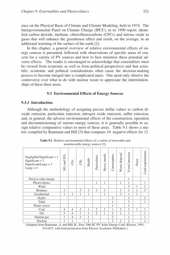
Chapter 9 Externalities and Photovoltaics 321
ence on the Physical Basis of Climate and Climate Modeling, held in 1974. TheIntergovernmental Panel on Climate Change (IPCC), in its 1990 report, identi-fied carbon dioxide, methane, chlorofluorocarbons (CFCs) and nitrous oxide asgases that will enhance the greenhouse effect and result, on the average, in anadditional warming of the surface of the earth [2].
In this chapter, a general overview of relative environmental effects of en-ergy sources is presented, followed with observations of specific areas of con-cern for a variety of PV sources and how to best minimize these potential ad-verse effects. The reader is encouraged to acknowledge that externalities mustbe viewed from economic as well as from political perspectives and that scien-tific, economic and political considerations often cause the decision-makingprocess to become merged into a complicated maze. One need only observe thecontroversy over what to do with nuclear waste to appreciate the interrelation-ships of these three areas.
9.3 Environmental Effects of Energy Sources
9.3.1 Introduction
Although the methodology of assigning precise dollar values to carbon di-oxide emission, particulate emission, nitrogen oxide emission, sulfur emission,and, in general, the adverse environmental effects of the construction, operationand decommissioning of various energy sources, it is generally possible to as-sign relative comparative values to most of these areas. Table 9.1 shows a ma-trix compiled by Baumann and Hill [3] that compares 10 negative effects for 12
Table 9.1 Relative environmental effects of a variety of renewable andnonrenewable energy sources [3].
Negligible/Significant = 1Significant = 2Significant/Large = 3Large = 4
SOx
and
NO
x
CO
2
CH
4
Hea
lth
Part
icul
ates
Hea
vy m
etal
s
Cat
astr
ophi
es
Was
te d
ispo
sal
Vis
ual i
ntru
sion
Noi
se
Lan
d re
quir
emen
ts
Passive solar energy 1Photovoltaics 1 1 1 1 1
Wind 3 1 1Biomass 1 3 1 1 1 1 1 1 3
Geothermal 1 1 1 1 1 2 1 1Hydro 2 3 3Tidal 1 3 1
Water waves 1 1Coal 4 4 2 1 2 2 1 2 2 1 3Oil 3 4 1 1 2 1 2 1 1 1
Natural gas 1 4 3 1 2 1 1Nuclear 1 1 1 2 3 2 1
(Adapted from Baumann, A. and Hill, R., Proc 10th EC PV Solar Energy Conf, Kluwer, 1991,834-837, with kind permission from Kluwer Academic Publishers.)
Photovoltaic Systems Engineering322
different energy sources with relative significances indicated. The observationsshould come as no particular surprise to anyone familiar with the listed sources.
9.3.2 Air Pollution
The U.S. Environmental Protection Agency (EPA) is required by the 1990amendment of the Clean Air Act [4] to regulate emissions of toxic air pollutantsfrom a published list of source categories. EPA is charged with setting stan-dards and with establishing and promulgating rules for reducing toxic emissionsto levels that meet the standards.
Each month, the EPA publishes on the worldwide web updated maps of non-attainment areas, i.e., those counties in the U.S. where certain pollutants exceedEPA limits [5]. The maps include nonattainment areas for CO, NO2, SO2, O3,Pb, and particulates of diameter less than 10 maps shows that certain parts of the country have significant areas of nonattain-ment for several of these pollutants.
EPA also has published a list of the top 25 sources of U.S. air pollution ineach of the six categories. A steel producer was at the top of the list of 25 emit-ters of NO2 on the March 1999 list. The remaining 24 entries were variouselectrical utilities, located predominantly along the Ohio River, where coal-firedgeneration is a major source of electricity. The map of the U.S. shows hundredsof NO2 emitters with annual emissions in excess of 100 tons, with emitters pres-ent in all 50 states.
Carbon monoxide is attributed mostly to steel companies, where carbon isused as a reducing agent to remove oxygen from the oxides of iron.
In March 1999, the top 25 producers of SO2 in the United States were allelectric utilities, with a total estimated production of 4.672 million tons per year.Every state in the union had SO2 emitters except Utah.
January 2003 ozone nonattainment areas covered a significant fraction ofCalifornia and a strip along the eastern seaboard from Washington, D.C., tosouthern Maine. Ozone is primarily a byproduct of internal combustion engines.Improving these engines or replacing much of the fleet, such as commuting ve-hicles with electric vehicles that run on PV-generated electricity from PV arraysin parking lots are two suggestions for reducing ozone emissions. Fuel cells asenergy sources for vehicles may be another promising solution. The hydrogenfor the fuel cells can be produced with PV-generated electricity.
Particulates with diameters less than 10 tend to remain airborne for relatively long periods of time, causing respiratoryproblems for anyone with sensitivities to certain particulates. Again, these con-taminants were at high levels in southern California, but also, surprisingly, in theGrand Canyon area, in southern Oregon and in northern Idaho and westernMontana. The 25 major fixed sources of PM-10 particles in the United Statesinclude steel mills and electric utility generators.
Although CO2 is recognized as a greenhouse gas, its emission is not offi-cially monitored or regulated at this time, although a move is underway to re-

Chapter 9 Externalities and Photovoltaics 323
duce CO2 emissions in the U.S. to 1990 levels as a result of the 1998 KyotoConference [6].
Readers are encouraged to visit the EPA web site for details of current EPAprograms. The World Resources Institute (WRI) maintains another web site thatprovides timely information on pollutants, including valuation methodologiesand economic cost discussions [7]. According to WRI, the IntergovernmentalPanel on Climate Change (IPCC) has calculated that to stabilize CO2 levels at1997 levels would require a 60% cut in emissions, maintained at that level forthe next century. Readers may also wish to review their solutions to the home-work problem in Chapter 1 that dealt with CO2 emissions from burning coal andpetroleum to put the CO2 from these sources into perspective.
Air quality is not a problem limited to the United States. As developingcountries continue to develop, often pollution controls take a back seat to devel-opment and the desires of the populations to have more energy at their disposal.Many of the world’s larger cities have severe air pollution problems.
The World Bank [8] has tabulated pollution indices for 83 large cities aroundthe world for 1995. In 1995, the highest levels of total suspended particulateswere found in Delhi, India (415 µg/m3), with Beijing, China, and Bombay, In-dia, following in close second and third place at 377 µg/m3 and 375 µg/m3. Incontrast, Stockholm, Sweden, had a level of 9 µg/m3.
The highest levels of SO2 occurred in Teheran, Iran (209 µg/m3). Rio de Ja-neiro, Brazil; Yokohama, Japan; Moscow, Russian Federation and Istanbul,Turkey also had concentrations in excess of 100 µg/m3.
The winner of the NO2 competition was Milan, Italy, with a concentration of248 µg/m3. Mexico City, Mexico, came in at 130 µg/m3, while Beijing, China,and Sofia, Bulgaria, both reported 122 µg/m3. New York City won the honorsfor the United States with 79 µg/m3. Havana, Cuba, was reported at 5 µg/m3.
For the reader who wishes to spend a year or two in the further collection ofinformation on air pollution, on February 2, 2003, a Netscape search for airpollution data netted 758,001 responses.
9.3.3 Water and Soil Pollution
Water pollution has perhaps received the most attention in the U.S. in termsof the lowering of pH of lakes in the Finger Lakes region of New York, pre-sumably caused by acid rain from SO2 and NO2 emissions in the Ohio Riverregion. The lowering of the pH as a result of the inability of the lakes to bufferthe effect of the acid rain, has been blamed for the loss of significant fish popu-lations. This loss has, in turn, resulted in a loss of revenue to other sectors ofsociety such as the sport fishing and tourist industries.
Other water pollution with perhaps more insidious consequences is the pol-lution of aquifers, lakes, rivers and streams with solid and liquid pollutants.While aquifer pollution has not been blamed on SO2 or NO2 or other atmos-pheric gases, it has been blamed on industrial solvents and other chemicals,many of which are used to support an economy with a large energy appetite.

Photovoltaic Systems Engineering324
Perhaps one of the best-known incidents in this category is the Love Canal, withmany other similar sites as identified for cleanup by the EPA. At this point, thecleanup costs of these toxic waste dumps is being quantified, so these costs canbe related back as externalities resulting from past waste-dumping practices.
It has been reported that soil acidification leads to permanently reduced pro-ductivity resulting from slower decomposition of humus and diminishing humusquality. Other important effects of soil acidification include leaching of alkaliand alkaline metals and release of heavy metals into soils. With changing qual-ity of the soil surrounding the roots of trees, it is believed that the trees may be-come more sensitive to gaseous air pollutants [9].
9.3.4 Infrastructure Degradation
A number of studies have shown that pollution causes premature degradationof infrastructure [10]. Stonework, carbon steel, nickel and nickel-plated steel,zinc and galvanized steel are all highly affected by sulfur dioxide in rain. It hasbeen estimated that in unpolluted environments, galvanized coatings last up tothree times longer, and in polluted areas galvanized transmission towers requirerepainting nearly twice as often. Hence, a cost figure can be attached to therestoration of structural finishes. However, assigning responsibility for the deg-radation is somewhat more problematic in that it is difficult to determine the mixof pollution sources that cause a specific amount of degradation to any particularsite, since the origin of any pollutant at any particular time will depend on thewind direction.
9.3.5 Quantifying the Cost of Externalities
The Cost of CO2
The cost of CO2 can be considered in two ways: the cost of controlling CO2
and the benefit of controlling CO2. This method is applicable to other pollutantsas well, but only CO2 will be discussed in this section.
According to the World Resources Institute, holding CO2 levels at 1990 lev-els will cost approximately 1 to 2% of the Gross Domestic Product for devel-oped countries over the long term, with reductions below 1990 levels cost in-creasing to 3%. An alternate analysis, however, suggests that by reducing CO2
levels significantly by incorporation of energy conservation measures, the costto reduce the CO2 levels will be less than the savings in energy costs.
If action is not taken to stop the increase of CO2 atmospheric concentration,it has been estimated that doubling of atmospheric CO2 will lead to an averagewarming of 2.5oC. According to current projections, this doubling will occurduring the next century if no curtailment measures are taken. In this case, it isestimated that the damage due to the warming will reach approximately 1 to1.5% of GDP per year in developed countries, with substantially more in islandnations. If CO2 levels continue to rise beyond the double point, the damage maycome closer to 6% of GDP.
Hence, it appears certain that damage will occur if nothing is done, while itis debatable whether there will be cost or cost savings if a program to reduce
Chapter 9 Externalities and Photovoltaics 325
CO2 levels is pursued. Considering that CO2 production is also generally ac-companied by the production of NO2, SO2 and particulates, if reduction of CO2
is also accompanied by reduction of other pollutants, then the benefits becomesubject to a multiplier effect. What is also being supported here is that it may bea better strategy to focus on reducing the production of CO2 rather than seques-tering CO2 already produced. Perhaps a carefully planned combination of thesetwo strategies may produce the most cost-effective results.
Sequestering CO2 With TreesIn order to quantify the cost of externalities, it is necessary to arrive at a
methodology for determining the value of a ton of SO2 or NO2 or CO2 or othersubstance. Since trees, other green plants and oceans have maintained the bal-ance between O2 and CO2 over the millennia, it would seem that a tree might bevalued in terms of the number of tons of CO2 it will remove from the atmos-phere in its lifetime. Since SO2 and NO2 generally are removed from the atmos-phere by rain, which dissolves them as weak acids, presumably a price per toncan be assigned in terms of the monetary value of any damage that may result tostructures or the environment from acid rain. For example, if a building requiresrepair more often as a result of acid rain, this is a measurable cost, provided thatthe increased repair costs can be documented. If the fish die in a lake as a resultof acid rain and, as a result, cause a decrease in tourism to the area, this also mayconstitute a documented cost if the source or sources can be identified.
The cost of CO2 and other pollutants can be measured in several ways, in-cluding the cost of repairing the damage, the cost of controlling the damage byreducing emission of pollutants and the cost of mitigating the damage, such asby absorbing the additional CO2 by trees. Hodas (1990) [11] reported costs of$240 per ton of carbon for removal of CO2 from exhaust gases, with significanttechnical difficulty. The scrubbed CO2 would then be liquefied and pumped to adepth of about 500 feet in the ocean, where it would then dissolve and becomeavailable for plankton and ocean vegetation. The cost of such an operationwould likely be close to $1000/kW for scrubbing and disposal. There would alsobe a 25% energy penalty, since the energy for the scrubbing and disposal wouldnot be available for other end users, as well as a 22% capacity penalty and addi-tional annual maintenance costs.
Supply, and, demand, side efficiency improvements are estimated to cost inthe range of $20 per ton of carbon avoided. Automobile efficiency increasesalso save 22 pounds of CO2 per gallon not burned, with an estimated cost of$0.53 per gallon for the effort required to increase automobile efficiency to 44miles per gallon, assuming continued use of gasoline as a fuel.
It is estimated that the U.S. would require 1.5 billion hectares of forest toabsorb its annual CO2 emissions [11]. The problem is that the total land area ofthe U.S. is only 913 million hectares, and forest in Death Valley, CA, and quitea few other areas appears as an unlikely prospect.
The idea of planting trees to mitigate the effects of CO2 generation was firstattempted in a project proposed by Applied Energy Service. This project in-
Photovoltaic Systems Engineering326
volved planting approximately 50 million trees in Costa Rica to mitigate theCO2 generated by a fossil fuel electric generator in Connecticut. The projectalso involved a fire protection program to save 2400 hectares of forest fromfires, with an overall estimated sequestering of 387,000 metric tons of carbonper year [11].
When trees are used for CO2 mitigation, it is necessary to consider what willbe done with the trees after they mature. If they are used for firewood, then thesequestered carbon is returned to its CO2 form. If they are used for construction,then the carbon remains sequestered. However, even if they are burned, on theassumption that something will be burned, the burning of these trees displacesburning of other trees. If the trees spared from fire are genetically diverse, thenan additional value can be assigned to preservation of diversity in the biosphere.
Perhaps an even more valuable location for trees is the urban environment,particularly in tropic or near-tropic regions. Hodas [11] observes that by plant-ing trees near buildings, the microclimate of the buildings is cooled by severaldegrees, thus reducing air conditioning needs and the corresponding energy re-quired for cooling. If the energy for cooling comes from fossil-fueled genera-tion, then the trees reduce atmospheric CO2 directly as a result of their photo-synthesis as well as indirectly by reducing the output demands and correspond-ing fuel requirements of the fossil-fueled generator.
The Hoff Clean Power EstimatorHoff [12] has developed a convenient computer program, available on the
internet, that estimates the annual amount of CO2 that can be avoided as a resultof using PV-generated electricity in place of electricity from fossil-fuel sources.The estimation procedure follows EPA guidelines. The program also producesan estimated net annual cost of a system on the basis of information keyed in bythe person running the program. Parameters used in the calculation include lo-cal electrical rates, income taxes, incentive programs, weather data, financingdetails and utility load profiles.
The net annual return on investment is calculated by taking the differencebetween loan payments and tax and utility bill savings. While the program doesnot take into account an economic value for the CO2 avoided, if an economiccost for CO2 were to be established, the program could readily include such cost,perhaps in the form of an additional tax credit, toward the annual net cost of thePV system. While an economic value has not yet been assigned to CO2, at thetime of this writing, NO2 and SO2 credits can now be purchased in the U.S. Ifthese costs, along with particulates and other air and water pollutants could beincluded in the Hoff Estimator, PV installations would more than likely becomeeven more economically attractive.
Attainment Levels as CommoditiesAnother interesting method of assigning value to pollutants comes as a con-
sequence of the Clean Air Act [4] and regulated attainment levels. Companiesare granted a certain allowable number of pollution units for their facilities. Forexample, an electrical generating utility may be allowed a certain number of
Chapter 9 Externalities and Photovoltaics 327
tons of SO2 emissions per year. If the utility does not generate as many tons asallowed, it may transfer the remainder of its allowed emissions to another entity.In a free enterprise society, this is not normally done as a simple, friendly ges-ture. Rather, air quality points are traded on the commodity exchange.
It is now possible for an individual, an organization or a company to pur-chase allowances for atmospheric SO2 and NO2 [13]. At the end of March eachyear, the U.S. Environmental Protection Agency holds an auction for SO2 allow-ances. Anyone can bid on the allowances, and the highest bidder gets the allow-ance. It is also possible to purchase allowances through a commodity broker orto purchase them through various environmental groups that purchase the allow-ances and then do not use them. Not using the allowances results in cleaner air.It is also possible to purchase NO2 allowances from brokers or from environ-mental groups, but they are not currently auctioned off by the EPA.
While this practice does not affix a price to emissions based on specific envi-ronmental costs, it at least shows that emissions do have some economic cost,and the reduction of emissions can result in economic benefit. What is interest-ing is that the law of supply and demand dictates the price of air quality points.If strict laws are enacted to reduce pollutants, companies end up investing inpollution control technologies, such as electrostatic precipitators and scrubbers.If these investments result in sufficient reduction in emission of pollutants, thena smaller number of air quality points will be needed and a larger number willbe available. This means the price will go down.
Other related actions have also been offered by energy producers in trade forpermission to operate, such as improving navigation channels to reduce the like-lihood of accidental fuel spills. These added costs represent the attachment of aprice to certain externalities, and, as a result, end up incorporating the costs ofthe externalities into the cost of the product.
SubsidiesSubsidies were included as components of direct costs of doing business in
Chapter 5, since they are usually included in the reduction of the cost of a prod-uct, such as energy, to the consumer. However, unless a level playing fieldexists, the costs of two energy sources cannot be properly compared. A levelplaying field exists when all energy sources are subsidized equally on a kWh-to-kWh basis. The difficulty is the identification of all subsidies, since some aredirect and others are indirect.
A direct subsidy, such as a depletion allowance, can be quantified in terms ofdollars per kWh. An indirect subsidy, such as military presence, can also some-times be quantified, but will normally not appear in the financial records of acompany. The effects of favorable tax considerations and tariffs can also bequantified in either a direct or indirect manner.
Government-sponsored research and government purchase of systems orrebates or tax credits on systems are also forms of subsidy. Generally, govern-ment involvement is justified on the basis that once the subsidized industry isable to compete without subsidy, it will generate sufficient revenues to result insufficient taxes to reimburse the government for its initial investment. In any
Photovoltaic Systems Engineering328
case, hardly an energy source exists that does not benefit to some extent fromsubsidies. To date, however, no one has requested a depletion allowance onsunlight, although solar access rights have been challenged in the case whereone party shades another party’s solar system.
9.3.6 Health and Safety as Externalities
Recent litigation against tobacco companies, resulting in the award of bil-lions of dollars in damages to states to help reimburse the costs of tobacco-related illnesses, has shown that the cost of public health is becoming a recog-nized externality, with a significant price tag. Other lawsuits have also beensuccessfully prosecuted against a variety of forms of pollution resulting fromcareless or indiscriminate disposal of many forms of toxic wastes. These casesconfirm the linkage between public health and its economic cost.
Public safety is also at issue when energy sources are considered. The Cher-nobyl and Three Mile Island nuclear accidents both brought to the forefrontpublic concern over nuclear safety. The location of large fuel tanks in highlypopulated areas also is of concern to public advocacy groups. Transport of vari-ous fuels is also problematic, especially when large tanker trucks are involved inaccidents that result in spilling of their contents and subsequent major efforts toclean up the damage before aquifers are affected. Even in the case of renewableenergy sources, concern has been expressed about the possibility of constructionaccidents, since installation of renewable sources tends to be more labor inten-sive per installed kW than conventional sources. Manufacture of the materialsused in conventional generation facilities carries with it both energy costs andmaterials costs, along with certain levels of exposure to hazardous or toxic mate-rials. Similar costs are associated with the manufacture of photovoltaic cellsand system components. Although these costs tend to be incorporated into theproduction cost of the materials, when toxic waste byproducts result, they areoften treated as externalities.
The balance of this chapter explores the externalities associated with theproduction, deployment, operation and decommissioning of PV power systems.Particular attention is paid to the environmental concerns associated with eachof the phases, recognizing that in order to produce PV systems, initially otherenergy sources must be exploited.
9.4 Externalities Associated with PV Systems
9.4.1 Environmental Effects of PV System Production
The production phase of each PV technology can be described in terms of aproduction cycle, which includes potential pollutants or hazardous waste associ-ated with each production step. Table 9.2 summarizes areas of environmental orhealth concern for current PV technologies that have promising possibilities forlarge scale production. The associated CO2 for each technology represents theCO2 resulting from the production of the primary energy used to produce the PV
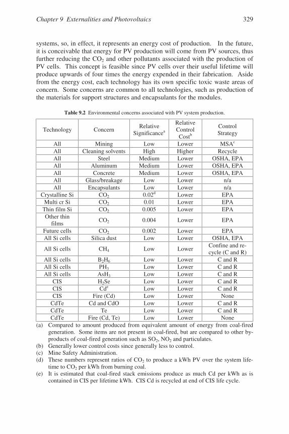
Chapter 9 Externalities and Photovoltaics 329
systems, so, in effect, it represents an energy cost of production. In the future,it is conceivable that energy for PV production will come from PV sources, thusfurther reducing the CO2 and other pollutants associated with the production ofPV cells. This concept is feasible since PV cells over their useful lifetime willproduce upwards of four times the energy expended in their fabrication. Asidefrom the energy cost, each technology has its own specific toxic waste areas ofconcern. Some concerns are common to all technologies, such as production ofthe materials for support structures and encapsulants for the modules.
Table 9.2 Environmental concerns associated with PV system production.
Technology ConcernRelative
Significancea
RelativeControlCostb
ControlStrategy
All Mining Low Lower MSAc
All Cleaning solvents High Higher RecycleAll Steel Medium Lower OSHA, EPAAll Aluminum Medium Lower OSHA, EPAAll Concrete Medium Lower OSHA, EPAAll Glass/breakage Low Lower n/aAll Encapsulants Low Lower n/a
Crystalline Si CO2 0.02d Lower EPAMulti cr Si CO2 0.01 Lower EPA
Thin film Si CO2 0.005 Lower EPAOther thin
filmsCO2 0.004 Lower EPA
Future cells CO2 0.002 Lower EPAAll Si cells Silica dust Low Lower OSHA, EPA
All Si cells CH4 Low LowerConfine and re-cycle (C and R)
All Si cells B2H6 Low Lower C and RAll Si cells PH3 Low Lower C and RAll Si cells AsH3 Low Lower C and R
CIS H2Se Low Lower C and RCIS Cde Low Lower C and RCIS Fire (Cd) Low Lower None
CdTe Cd and CdO Low Lower C and RCdTe Te Low Lower C and RCdTe Fire (Cd, Te) Low Lower None
(a) Compared to amount produced from equivalent amount of energy from coal-firedgeneration. Some items are not present in coal-fired, but are compared to other by-products of coal-fired generation such as SO2, NO2 and particulates.
(b) Generally lower control costs since generally less to control.(c) Mine Safety Administration.(d) These numbers represent ratios of CO2 to produce a kWh PV over the system life-
time to CO2 per kWh from burning coal.(e) It is estimated that coal-fired stack emissions produce as much Cd per kWh as is
contained in CIS per lifetime kWh. CIS Cd is recycled at end of CIS life cycle.
Photovoltaic Systems Engineering330
Perhaps the most important common denominator associated with all tech-nologies is the material used for cleaning the cells. In all cases, high levels ofcleanliness are required to maximize performance, and in some cases the sol-vents used are highly toxic. Fortunately these solvents have been in commonuse in the semiconductor industry and careful means of control are well under-stood within the industry. The common means of dealing with these solvents isto confine them and then recycle them.
In the case of Si PV cells, the most significant concerns are the proper han-dling of the dopants for n-type and p-type. Since the semiconductor industry hasbeen handling these components effectively, the processes are well defined.Once the impurities are in the Si, the amounts are so insignificant that the dopedSi is considered to be benign.
For the CIS cells and the CdTe cells, the Cd content is the primary item ofconcern, but since the films in these devices are generally less than 2 the total amount of Cd and Te in these cells is very small. Another concern forCIS is the use of H2Se for the deposit of Se into the cell, but again, the use ofthis highly toxic substance can be kept well under control with minimal risk ofhaving it escape into the environment.
9.4.2 Environmental Effects of PV System Deployment and Operation
The deployment of PV systems has associated environmental and healthcosts similar to the deployment of other energy technologies [14]. Steel, alumi-num and concrete can be expected to be part of the structures upon which thePV arrays and associated BOS components will be mounted. Hence, the pro-duction costs and associated environmental costs, such as CO production in thereduction of iron oxides, become associated with PV deployment.
Just as construction accidents occur in any construction project, it is antici-pated that PV project construction will also result in construction accidents. Forthe most part, materials used in construction of PV facilities are nontoxic. It isthus the responsibility of the installation contractor to ensure that the workplaceand work practices follow Occupational Safety and Health Administration(OSHA) rules.
Once the PV system is installed, it quietly generates pollution-free electricityany time the sun is shining. The main environmental concern associated withthe operation of PV systems is if a system containing Cd or Se or Te should beexposed to fire. Analysis has shown, however, that since these materials appearin such minute quantities in thin-film PVs that anyone approaching close enoughto encounter significant exposure to any of the toxins would face significantlymore danger from the fire itself. For example, only 400 g of Cd are present in a1 MW CIS PV system, whereas 5 g/m2 of Cd are present in CdTe systems, orabout 25 times the amount in CIS systems.
Other dangers associated with the installed system include, of course, thepossibility of electrical shock or fire. Systems installed in accordance with theNational Electrical Code [15] will reduce any shock or fire hazard to a mini-
Chapter 9 Externalities and Photovoltaics 331
mum, both for the general public as well as maintenance personnel. The factthat PV systems are inherently current limiting tends to reduce their potential toproduce high-current arcing if they are inadvertently shorted. Incorporation ofground fault protection in residential rooftop systems adds further protection.
A final safety consideration for installed PV systems relates to their ability towithstand high winds. Inadequately mounted PV modules in high winds maytear loose from their mounting and becoming projectiles. Installations compli-ant with local building code wind-loading requirements present minimal risk.
9.4.3 Environmental Effects of PV System Decommissioning
Certain regulatory requirements apply to the decommissioning of PV sys-tems. Assuming that the system will be disassembled at the end of its usefullifetime, it is then necessary to consider the destination of the disassembledcomponents. Some of the components will require disposal according to toxicwaste regulations unless they can be recycled, and other components will not besubject to quite as stringent requirements.
The Resource and Conservation Recovery Act constitutes the primary set ofrules governing wastes containing Cd, Se, Pb, Cu or Ag provided that thesewastes are considered to be discarded material and are not included in any spe-cific exclusions [16]. The EPA defines the Toxicity Characteristic LeachingProcedure (TCLP) for 39 materials to determine whether waste products con-taining them may be classified as hazardous. Any waste product containing anyof the 39 materials that yields a soluble concentration in excess of its TCLP lim-its is considered hazardous.
The California Hazardous Waste Control Law introduces an additional testfor toxicity characterization, with two additional indicators. The Waste Extrac-tion Test (WET) is used to identify non-RCRA toxic wastes. The WET thresh-old limits are defined as the Soluble Threshold Limit Concentration (STLC) andthe Total Threshold Limit Concentration (TTLC), that is the total concentrationof listed materials, in any form.
In terms of STLC and TTLC, it appears that CdTe modules may be charac-terized as hazardous in terms of TTLC and STLC for Cd. CIS modules may besubject to TTLC for Se and STLC for Se and Cd. Polycrystalline Si modulesmay have a problem with TTLC and STLC for Ag or Pb. In some cases, Pb andCu may be a problem, and a-Si:H modules do not seem to have any toxicityproblems [16]. If CdTe and CIS modules are recycled, they are exempt fromthe disposal regulations. Studies have projected recycling costs of approxi-mately $0.01 to $0.04 per watt for both materials, using relatively standard sepa-ration techniques.
Photovoltaic Systems Engineering332
Problems
9.1 Look up the U.S. nonattainment regions on the U.S. Environmental Protec-tion Agency web site.
9.2 If recycling of CdTe PV modules will cost approximately $0.04/watt andthe lifetime of a CdTe module is 20 years, what is the present value of therecycling cost for a 10 kW array?
9.3 Determine the prices of a ton of SO2 and a ton of NO2 on the commodityexchange. The EPA website lists websites and phone numbers of commod-ity brokers and environmental organizations that purchase and sell them.
9.4 If burning a gallon of gasoline produces 22 pounds of CO2, estimate theCO2 that your vehicle emits in a year. Compare this with the amount thatwould have been generated had you been driving an electric vehicle chargedfrom a PV array or a hybrid auto or a fuel cell–powered auto. Take into ac-count the origin of the H2 used in the fuel cell.
9.5 In the CO2 scrubbing and liquefaction scheme reported by Hodas, estimatethe increase in electrical cost that would be necessary to offset the cost ofthe process.
9.6 Use the Hoff Clean Power Estimator [12] to determine for your residentialzip code area:a. A combination of system cost per PV watt (at STC), interest rate andloan duration that will result in a positive net annual cash flow for a PVsystem owner of your income level and marital status.b. Assume the cost of a PV system to be $3/watt and the annual interestrate on a 25-year loan for the PV system to be 6%. Determine the necessaryvalue of a ton of avoided CO2 to bring the annual system net cost to zero foryour personal income and tax situation (or your hypothetical income and taxsituation).
References
[1] Moore, T. G., Climate of Fear: Why We Shouldn’t Worry about Global Warming,the Cato Institute, Washington, D.C., 1998.
[2] Paterson, M., Global Warming and Global Politics, Routledge, London, 1996. [3] Baumann, A. and Hill, R., Proc. 10th EC Photovoltaics Solar Energy Conference,
Kluwer, Dordrecht, 1991, 834−837. [4] 42 U. S. C. § 7401 et. seq. (Clean Air Act).

Chapter 9 Externalities and Photovoltaics 333
[5] wysiwyg://180//www.epa.gov/airprogm/airs/data/mapview.htm (EPA air pollutionmaps).
[6] 3rd Conference of the Parties to the U. N. Framework Convention on ClimateChange, Kyoto, Japan, December 1997.
[7] http://www.wri.org/wr-96-97/ac_txt6.html (World Resources Institute). [8] www.worldbank.org/nipr/wdi98/tables3.12.pdf (World Bank pollution data). [9] Guderian, R., External Environmental Costs of Electric Power, Springer-Verlag,
Berlin, 1990, 9−24.[10] Weltschev, M., External Environmental Costs of Electric Power, Springer-Verlag,
Berlin, 1990, 25−35.[11] Hodas, D. R., External Environmental Costs of Electric Power, Springer-Verlag,
Berlin, 1990, 59−78.[12] www.clean-power.com/estimator/ (The Hoff Clean Power Estimator Program).[13] http://www.epa.gov/airmarkt/trading/buying.html (Information on SO2 and NO2
commodity trading).[14] Markvart, T., Ed., Solar Electricity, John Wiley & Sons, Chichester, U.K., 1994.[15] NFPA 70 National Electrical Code, 2002 Edition, National Fire Protection Associa-
tion, Quincy, MA, 2002.[16] Fthenakis, V. M. and Moskowitz, P. D., Emerging photovoltaic technologies: envi-
ronmental and health issues update, NREL/SNL Photovoltaics Program Review,AIP Press, New York, 1997.
335
Chapter 10THE PHYSICS OF PHOTOVOLTAIC CELLS
10.1 Introduction
By this point, it is possible that the reader, now highly skilled at PV systemdesign, might be interested in what goes on inside the PV cell during the processof converting light energy into electrical energy. This chapter is presented withthe purpose of enabling the reader to become familiar with the challenges facingthose engineers and physicists who spend their lives working on processes andmaterials aimed at reducing the cost and increasing the efficiency of PV cells.Initially, the basics of PV energy conversion are presented, followed by discus-sion of present limitations of cell production and some of the ideas that haveemerged toward overcoming these limitations. Most readers will have alreadyhad at least an exposure to the theory of operation of the pn junction and thesemiconductor diode in an electronics course, so it will be assumed that thereader will at least be familiar with the basic diode equation.
10.2 Optical Absorption
10.2.1 Introduction
When light shines on a material, it is either reflected, transmitted, or ab-sorbed. Absorption of light is simply the conversion of the energy contained inthe incident photon to some other form of energy, typically heat. Some materials,however, happen to have just the right properties needed to convert the energy inthe incident photons to electrical energy.
When a photon is absorbed, it interacts with an atom in the absorbing mate-rial by giving off its energy to an electron in the material. This energy transfer isgoverned by the rules of conservation of momentum and conservation of energy.Since the zero mass photon has very small momentum compared to the electronsand holes, the transfer of energy from a photon to a material occurs with incon-sequential momentum transfer. Depending on the energy of the photon, an elec-tron may be raised to a higher energy state within an atom or it may be liberatedfrom the atom. Liberated electrons are then capable of moving through the crys-tal in accordance with whatever phenomena may be present that could cause theelectron to move, such as temperature, diffusion or an electric field.
10.2.2 Semiconductor Materials
Semiconductor materials are characterized as being perfect insulators at ab-solute zero temperature, with charge carriers being made available for conduc-tion as the temperature of the material is increased. This phenomenon can be
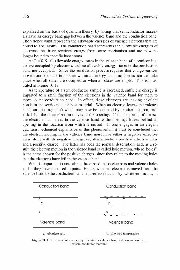
Photovoltaic Systems Engineering336
explained on the basis of quantum theory, by noting that semiconductor materi-als have an energy band gap between the valence band and the conduction band.The valence band represents the allowable energies of valence electrons that arebound to host atoms. The conduction band represents the allowable energies ofelectrons that have received energy from some mechanism and are now nolonger bound to specific host atoms.
At T = 0 K, all allowable energy states in the valence band of a semiconduc-tor are occupied by electrons, and no allowable energy states in the conductionband are occupied. Since the conduction process requires that charge carriersmove from one state to another within an energy band, no conduction can takeplace when all states are occupied or when all states are empty. This is illus-trated in Figure 10.1a.
As temperature of a semiconductor sample is increased, sufficient energy isimparted to a small fraction of the electrons in the valence band for them tomove to the conduction band. In effect, these electrons are leaving covalentbonds in the semiconductor host material. When an electron leaves the valenceband, an opening is left which may now be occupied by another electron, pro-vided that the other electron moves to the opening. If this happens, of course,the electron that moves in the valence band to the opening, leaves behind anopening in the location from which it moved. If one engages in an elegantquantum mechanical explanation of this phenomenon, it must be concluded thatthe electron moving in the valence band must have either a negative effectivemass along with its negative charge, or, alternatively, a positive effective massand a positive charge. The latter has been the popular description, and, as a re-sult, the electron motion in the valence band is called hole motion, where “holes”is the name chosen for the positive charges, since they relate to the moving holesthat the electrons have left in the valence band.
What is important to note about these conduction electrons and valence holesis that they have occurred in pairs. Hence, when an electron is moved from thevalence band to the conduction band in a semiconductor by whatever means, it
J
J
RRR RRR
R
Figure 10.1 Illustration of availability of states in valence band and conduction bandfor semiconductor material.
a. Absolute zero b. Elevated temperature
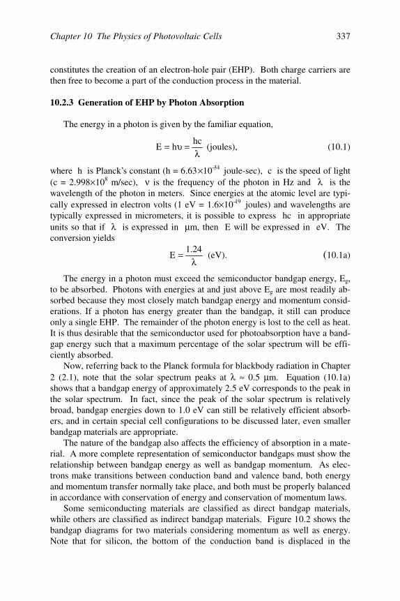
Chapter 10 The Physics of Photovoltaic Cells 337
constitutes the creation of an electron-hole pair (EHP). Both charge carriers arethen free to become a part of the conduction process in the material.
10.2.3 Generation of EHP by Photon Absorption
The energy in a photon is given by the familiar equation,
λ=υ= hc
hE (joules), (10.1)
where h is Planck’s constant (h = 6.63 × 10⁻³⁴ joule-sec), c is the speed of light(c = 2.998 × 10⁸ m/sec), ν is the frequency of the photon in Hz and λ is thewavelength of the photon in meters. Since energies at the atomic level are typi-cally expressed in electron volts (1 eV = 1.6 × 10⁻¹⁹ joules) and wavelengths aretypically expressed in micrometers, it is possible to express hc in appropriateunits so that if λ is expressed in µ m, then E will be expressed in eV. Theconversion yields
λ= 24.1
E (eV). (10.1a)
The energy in a photon must exceed the semiconductor bandgap energy, Eg,to be absorbed. Photons with energies at and just above Eg are most readily ab-sorbed because they most closely match bandgap energy and momentum consid-erations. If a photon has energy greater than the bandgap, it still can produceonly a single EHP. The remainder of the photon energy is lost to the cell as heat.It is thus desirable that the semiconductor used for photoabsorption have a band-gap energy such that a maximum percentage of the solar spectrum will be effi-ciently absorbed.
Now, referring back to the Planck formula for blackbody radiation in Chapter2 (2.1), note that the solar spectrum peaks at λ ≈ 0.5 µ m. Equation (10.1a)shows that a bandgap energy of approximately 2.5 eV corresponds to the peak inthe solar spectrum. In fact, since the peak of the solar spectrum is relativelybroad, bandgap energies down to 1.0 eV can still be relatively efficient absorb-ers, and in certain special cell configurations to be discussed later, even smallerbandgap materials are appropriate.
The nature of the bandgap also affects the efficiency of absorption in a mate-rial. A more complete representation of semiconductor bandgaps must show therelationship between bandgap energy as well as bandgap momentum. As elec-trons make transitions between conduction band and valence band, both energyand momentum transfer normally take place, and both must be properly balancedin accordance with conservation of energy and conservation of momentum laws.
Some semiconducting materials are classified as direct bandgap materials,while others are classified as indirect bandgap materials. Figure 10.2 shows thebandgap diagrams for two materials considering momentum as well as energy.Note that for silicon, the bottom of the conduction band is displaced in the
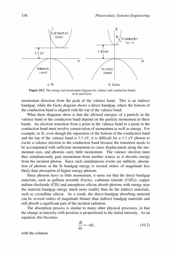
Photovoltaic Systems Engineering338
momentum direction from the peak of the valence band. This is an indirectbandgap, while the GaAs diagram shows a direct bandgap, where the bottom ofthe conduction band is aligned with the top of the valence band.
What these diagrams show is that the allowed energies of a particle in thevalence band or the conduction band depend on the particle momentum in thesebands. An electron transition from a point in the valence band to a point in theconduction band must involve conservation of momentum as well as energy. Forexample, in Si, even though the separation of the bottom of the conduction bandand the top of the valence band is 1.1 eV, it is difficult for a 1.1 eV photon toexcite a valence electron to the conduction band because the transition needs tobe accompanied with sufficient momentum to cause displacement along the mo-mentum axis, and photons carry little momentum. The valence electron mustthus simultaneously gain momentum from another source as it absorbs energyfrom the incident photon. Since such simultaneous events are unlikely, absorp-tion of photons at the Si bandgap energy is several orders of magnitude lesslikely than absorption of higher energy photons.
Since photons have so little momentum, it turns out that the direct bandgapmaterials, such as gallium arsenide (GaAs), cadmium teluride (CdTe), copperindium diselenide (CIS) and amorphous silicon absorb photons with energy nearthe material bandgap energy much more readily than do the indirect materials,such as crystalline silicon. As a result, the direct-bandgap absorbing materialcan be several orders of magnitude thinner than indirect bandgap materials andstill absorb a significant part of the incident radiation.
The absorption process is similar to many other physical processes, in thatthe change in intensity with position is proportional to the initial intensity. As anequation, this becomes
Idx
dI α−= , (10.2)
with the solution
(
S
(
S
H9H9
&RQGXFWLRQ
EDQG&RQGXFWLRQ
EDQG
9DOHQFH
EDQG9DOHQFH
EDQG
a. Si b. GaAs
Figure 10.2 The energy and momentum diagram for valence and conduction bandsin Si and GaAs.
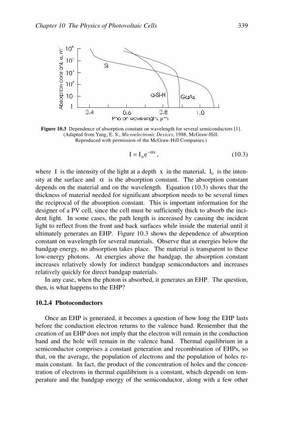
Chapter 10 The Physics of Photovoltaic Cells 339
xoeII α−= , (10.3)
where I is the intensity of the light at a depth x in the material, Io is the inten-sity at the surface and α is the absorption constant. The absorption constantdepends on the material and on the wavelength. Equation (10.3) shows that thethickness of material needed for significant absorption needs to be several timesthe reciprocal of the absorption constant. This is important information for thedesigner of a PV cell, since the cell must be sufficiently thick to absorb the inci-dent light. In some cases, the path length is increased by causing the incidentlight to reflect from the front and back surfaces while inside the material until itultimately generates an EHP. Figure 10.3 shows the dependence of absorptionconstant on wavelength for several materials. Observe that at energies below thebandgap energy, no absorption takes place. The material is transparent to theselow-energy photons. At energies above the bandgap, the absorption constantincreases relatively slowly for indirect bandgap semiconductors and increasesrelatively quickly for direct bandgap materials.
In any case, when the photon is absorbed, it generates an EHP. The question,then, is what happens to the EHP?
10.2.4 Photoconductors
Once an EHP is generated, it becomes a question of how long the EHP lastsbefore the conduction electron returns to the valence band. Remember that thecreation of an EHP does not imply that the electron will remain in the conductionband and the hole will remain in the valence band. Thermal equilibrium in asemiconductor comprises a constant generation and recombination of EHPs, sothat, on the average, the population of electrons and the population of holes re-main constant. In fact, the product of the concentration of holes and the concen-tration of electrons in thermal equilibrium is a constant, which depends on tem-perature and the bandgap energy of the semiconductor, along with a few other
3KRWRQZDYHOHQJWK Pµ
$EVRUSWLRQFRQVWDQW
P
α, −
6L
D6L+ *D$V
Figure 10.3 Dependence of absorption constant on wavelength for several semiconductors [1].(Adapted from Yang, E. S., , 1988, McGraw-Hill.
Reproduced with permission of the McGraw-Hill Companies.)Microelectronic Devices
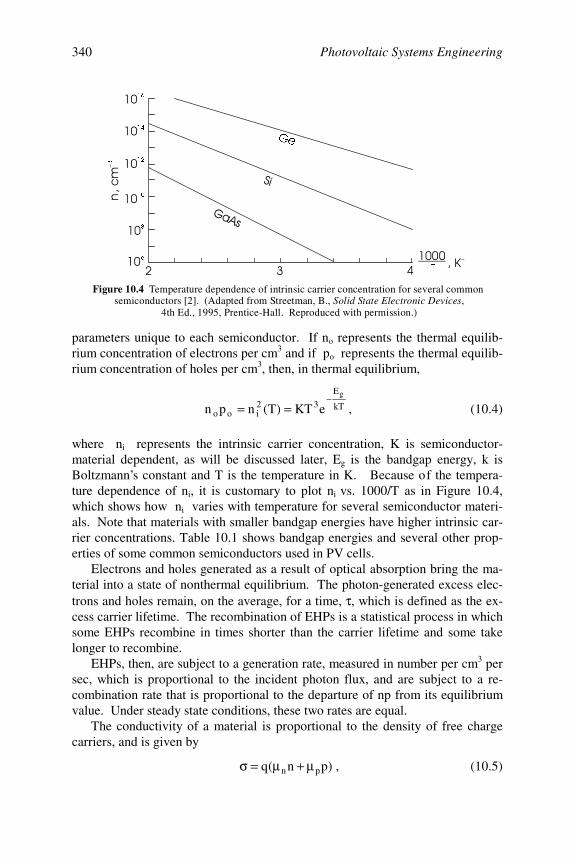
Photovoltaic Systems Engineering340
parameters unique to each semiconductor. If no represents the thermal equilib-rium concentration of electrons per cm3 and if po represents the thermal equilib-rium concentration of holes per cm3, then, in thermal equilibrium,
kT
E32
ioo
g
eKT)T(npn−
== , (10.4)
where ni represents the intrinsic carrier concentration, K is semiconductor-material dependent, as will be discussed later, Eg is the bandgap energy, k isBoltzmann’s constant and T is the temperature in K. Because of the tempera-ture dependence of ni, it is customary to plot ni vs. 1000/T as in Figure 10.4,which shows how ni varies with temperature for several semiconductor materi-als. Note that materials with smaller bandgap energies have higher intrinsic car-rier concentrations. Table 10.1 shows bandgap energies and several other prop-erties of some common semiconductors used in PV cells.
Electrons and holes generated as a result of optical absorption bring the ma-terial into a state of nonthermal equilibrium. The photon-generated excess elec-trons and holes remain, on the average, for a time, τ , which is defined as the ex-cess carrier lifetime. The recombination of EHPs is a statistical process in whichsome EHPs recombine in times shorter than the carrier lifetime and some takelonger to recombine.
EHPs, then, are subject to a generation rate, measured in number per cm3 persec, which is proportional to the incident photon flux, and are subject to a re-combination rate that is proportional to the departure of np from its equilibriumvalue. Under steady state conditions, these two rates are equal.
The conductivity of a material is proportional to the density of free chargecarriers, and is given by
)pn(q pn µ+µ=σ , (10.5)
*H
7−
L
−
Figure 10.4 Temperature dependence of intrinsic carrier concentration for several common semiconductors [2]. (Adapted from Streetman, B., ,
4th Ed., 1995, Prentice-Hall. Reproduced with permission.)Solid State Electronic Devices
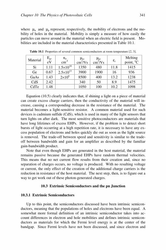
Chapter 10 The Physics of Photovoltaic Cells 341
where µ n and µ p represent, respectively, the mobility of electrons and the mo-bility of holes in the material. Mobility is simply a measure of how easily theparticles can move around in the material when an electric field is present. Mo-bilities are included in the material characteristics presented in Table 10.1.
Table 10.1 Properties of several common semiconductors at room temperature [2, 3].
MaterialEg,eV
ni,cm–3
µ n,cm2/Vs
µ p,cm2/Vs
ε rMeltingpoint, oC
Si 1.11 1.5 × 10¹⁰ 1350 480 11.8 1415Ge 0.67 2.5 × 10¹³ 3900 1900 16 936
GaAs 1.43 2 × 10⁶ 8500 400 13.2 1238CdS 2.42 340 50 8.9 1475
CdTe 1.48 1050 100 10.2 1098
Equation (10.5) clearly indicates that, if shining a light on a piece of materialcan create excess charge carriers, then the conductivity of the material will in-crease, causing a corresponding decrease in the resistance of the material. Thematerial becomes a light-sensitive resistor. A common material used for suchdevices is cadmium sulfide (CdS), which is used in many of the light sensors thatturn lights on after dark. The most sensitive photoconductors are materials thathave long lifetimes of excess EHPs. However, if the problem is to detect shortbursts of light occurring at a high repetition rate, it is necessary to have any ex-cess population of electrons and holes quickly die out as soon as the light sourceis removed. The trade-off between speed and sensitivity is similar to the trade-off between bandwidth and gain for an amplifier as described by the familiargain-bandwidth product.
Note that even though EHPs are generated in the host material, the materialremains passive because the generated EHPs have random thermal velocities.This means that no net current flow results from their creation and, since noseparation of charges occurs, no voltage is produced. With no resulting voltageor current, the only effect of the creation of the additional charge carriers is thereduction in resistance of the host material. The next step, then, is to figure out away to get work out of these photon-generated charges.
10.3 Extrinsic Semiconductors and the pn Junction
10.3.1 Extrinsic Semiconductors
Up to this point, the semiconductors discussed have been intrinsic semicon-ductors, meaning that the populations of holes and electrons have been equal. Asomewhat more formal definition of an intrinsic semiconductor takes into ac-count differences in electron and hole mobilities and defines intrinsic semicon-ductors as materials for which the Fermi level energy is at the center of thebandgap. Since Fermi levels have not been discussed, and since electron and

Photovoltaic Systems Engineering342
hole mobilities are generally close enough to keep the Fermi level quite close tothe center of the bandgap, the equal carrier definition will suffice for the follow-ing discussion. The reader is referred to a text on semiconductor device physicsfor more details on Fermi levels [1, 2].
At T = 0 K, intrinsic semiconductors have all covalent bonds completed withno leftover electrons or holes. If certain impurities are introduced into intrinsicsemiconductors, there can be leftover electrons or holes at T = 0 K. For exam-ple, consider silicon, which is a group IV element, which covalently bonds withfour nearest neighbor atoms to complete the outer electron shells of all the at-oms. At T = 0 K, all the covalently bonded electrons are in place, whereas atroom temperature, about one in 1012 of these covalent bonds will break, formingan EHP, resulting in minimal charge carriers for current flow.
If, however, phosphorous, a group V element, is introduced into the siliconin small quantities, such as one part in 106, four of the valence electrons of thephosphorous atoms will covalently bond to the neighboring silicon atoms, whilethe fifth valence electron will have no electrons with which to covalently bond.This fifth electron remains weakly coupled to the phosphorous atom, readilydislodged by temperature, since it requires only 0.04 eV to excite the electronfrom the atom to the conduction band. At room temperature, sufficient thermalenergy is available to dislodge essentially all of these extra electrons from thephosphorous impurities. These electrons thus enter the conduction band underthermal equilibrium conditions, and the concentration of electrons in the con-duction band becomes nearly equal to the concentration of phosphorous atoms,since the impurity concentration is normally on the order of 108 times larger thanthe intrinsic carrier concentration.
Since the phosphorous atoms donate electrons to the material, they are calleddonor atoms and are represented by the concentration, ND. Note that the phos-phorous, or other group V impurities, do not add holes to the material. Theyonly add electrons. They are thus designated as n-type impurities.
On the other hand, if group III atoms such as boron are added to the intrinsicsilicon, they have only three valence electrons to covalently bond with nearestsilicon neighbors. The missing covalent bond appears the same as a hole, whichcan be released to the material with a small amount of thermal energy. Again, atroom temperature, nearly all of the available holes from the group III impurityare donated to the conduction process in the host material. Since the concentra-tion of impurities will normally be much larger than the intrinsic carrier concen-tration, the concentration of holes in the material will be approximately equal tothe concentration of impurities.
Historically, group III impurities in silicon have been viewed as electron ac-ceptors, which, in effect, donate holes to the material. Rather than being termedhole donors, however, they have been called acceptors. Thus, acceptor impuri-ties donate holes, but no electrons, to the material and the resulting hole densityis approximately equal to the density of acceptors, which is represented as NA.Figure 10.5 shows the effects of donor and acceptor impurities on the intrinsic
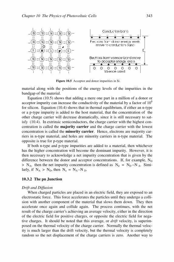
Chapter 10 The Physics of Photovoltaic Cells 343
material along with the positions of the energy levels of the impurities in thebandgap of the material.
Equation (10.5) shows that adding a mere one part in a million of a donor oracceptor impurity can increase the conductivity of the material by a factor of 108
for silicon. Equation (10.4) shows that in thermal equilibrium, if either an n-typeor a p-type impurity is added to the host material, that the concentration of theother charge carrier will decrease dramatically, since it is still necessary to sat-isfy (10.4). In extrinsic semiconductors, the charge carrier with the highest con-centration is called the majority carrier and the charge carrier with the lowestconcentration is called the minority carrier. Hence, electrons are majority car-riers in n-type material, and holes are minority carriers in n-type material. Theopposite is true for p-type material.
If both n-type and p-type impurities are added to a material, then whicheverhas the higher concentration will become the dominant impurity. However, it isthen necessary to acknowledge a net impurity concentration that is given by thedifference between the donor and acceptor concentrations. If, for example, ND
> NA, then the net impurity concentration is defined as Nd = ND – N A. Simi-larly, if NA > ND, then Na = NA – N D.
10.3.2 The pn Junction
Drift and DiffusionWhen charged particles are placed in an electric field, they are exposed to an
electrostatic force. This force accelerates the particles until they undergo a colli-sion with another component of the material that slows them down. They thenaccelerate once again and collide again. The process continues, with the netresult of the charge carrier’s achieving an average velocity, either in the directionof the electric field for positive charges, or opposite the electric field for nega-tive charges. It should be noted that this average, or drift velocity, is superim-posed on the thermal velocity of the charge carrier. Normally the thermal veloc-ity is much larger than the drift velocity, but the thermal velocity is completelyrandom so the net displacement of the charge carriers is zero. Another way to
6L 6L 6L 6L 6L
6L 6L 6L
6L 6L 6L 6L 6L
6L 6L 6L 6L 6L
6L 6L 6L 6L 6L
(J
&RQGXFWLRQEDQG
WRDFFHSWRUHQHUJ\OHYHOV
9DOHQFHEDQG
(OHFWURQVIURPYDOHQFHEDQGPRYH
(OHFWURQVIURPGRQRUHQHUJ\OHYHOVPRYHWRFRQGXFWLRQEDQG
Figure 10.5 Acceptor and donor impurities in Si.
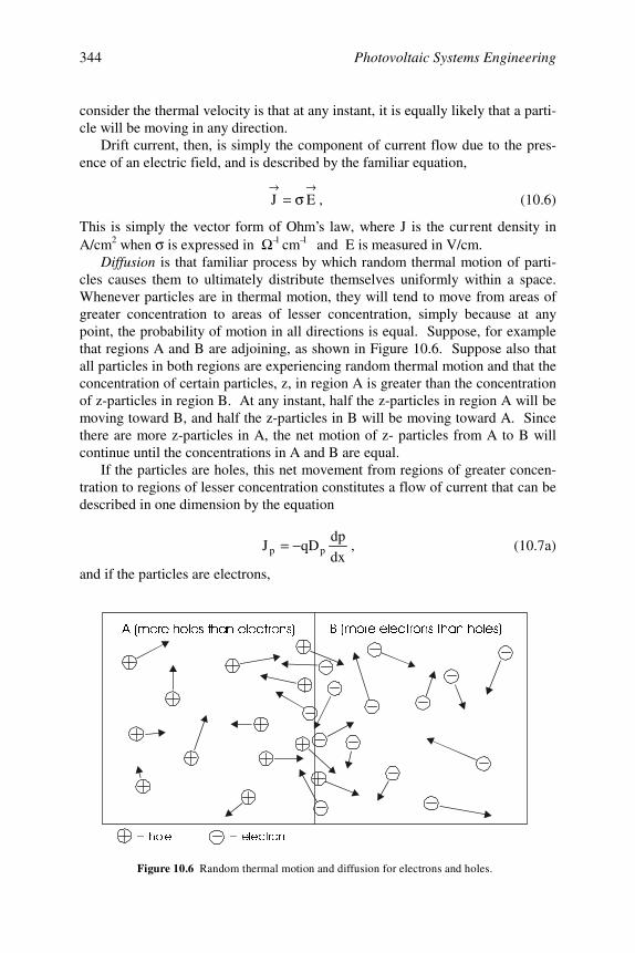
Photovoltaic Systems Engineering344
consider the thermal velocity is that at any instant, it is equally likely that a parti-cle will be moving in any direction.
Drift current, then, is simply the component of current flow due to the pres-ence of an electric field, and is described by the familiar equation,
→→σ= EJ , (10.6)
This is simply the vector form of Ohm’s law, where J is the current density inA/cm2 when σ is expressed in Ω –1 cm–1 and E is measured in V/cm.
Diffusion is that familiar process by which random thermal motion of parti-cles causes them to ultimately distribute themselves uniformly within a space.Whenever particles are in thermal motion, they will tend to move from areas ofgreater concentration to areas of lesser concentration, simply because at anypoint, the probability of motion in all directions is equal. Suppose, for examplethat regions A and B are adjoining, as shown in Figure 10.6. Suppose also thatall particles in both regions are experiencing random thermal motion and that theconcentration of certain particles, z, in region A is greater than the concentrationof z-particles in region B. At any instant, half the z-particles in region A will bemoving toward B, and half the z-particles in B will be moving toward A. Sincethere are more z-particles in A, the net motion of z- particles from A to B willcontinue until the concentrations in A and B are equal.
If the particles are holes, this net movement from regions of greater concen-tration to regions of lesser concentration constitutes a flow of current that can bedescribed in one dimension by the equation
dxdp
qDJ pp −= , (10.7a)
and if the particles are electrons,
$PRUHKROHVWKDQHOHFWURQV %PRUHHOHFWURQVWKDQKROHV
KROH HOHFWURQ
Figure 10.6 Random thermal motion and diffusion for electrons and holes.
Chapter 10 The Physics of Photovoltaic Cells 345
dxdn
qDJ nn = . (10.7b)
In (10.7a) and (10.7b) the change in concentration with position is known as theconcentration gradient and Dp and Dn are the hole diffusion constant and theelectron diffusion constant, respectively. The minus sign in (10.7a) accounts forthe fact that if the gradient is negative, the holes flow in the positive x-direction.The lack of the minus sign in (10.7b) accounts for the fact that if electrons flowin the positive x-direction, the associated current is in the negative x-direction.In each case, q = 1.6 × 10⁻¹⁹ coulomb.
At this point, all that is necessary is to make two additional observations. Thefirst observation is that donor and acceptor atoms become donor and acceptorions when they give up their electron or hole to the host material. These ions arefixed in position in the host by covalent bonds. The second observation is that ineither n-type material or in p-type material, any point in the material will havecharge neutrality. That is, the net charge present at any point is zero due topositive charges being neutralized by negative charges. However, when n-typeand p-type materials are joined to form a pn junction, something special happensat the boundary.
Junction Formation and Built-In PotentialAlthough n-type and p-type materials are interesting and useful, the real fun
starts when a junction is formed between n-type and p-type materials. The pnjunction is treated in gory detail in most semiconductor device textbooks. Here,the need is to establish the foundation for the establishment of an electric fieldacross a pn junction and to note the effect of this electric field on photo-generated EHPs.
Figure 10.7 shows a pn junction formed by placing p-type impurities on oneside and n-type impurities on the other side. There are many ways to accomplishthis structure. The most common is the diffused junction.
To form a diffused pn junction, the host material is grown with impurities, soit will be either n-type or p-type. The material is either grown or sliced into anappropriate thickness. Then the material is heated in the presence of the oppo-site impurity, which is usually in the form of a gas. This impurity will diffuseinto the host material at a level that exceeds the host impurity level, but will onlypenetrate a small distance into the host material, depending on how long the hostmaterial is left at the elevated temperature. The result is a layer of material ofone dominant impurity on top of the remainder of the material, which is dopedwith the other dominant impurity.
When the two materials are brought together, the first thing to happen is thatthe conduction electrons on the n-side of the junction notice the scarcity of con-duction electrons on the p-side, and the valence holes on the p-side notice thescarcity of valence holes on the n-side. Since both types of charge carrier areundergoing random thermal motion, they begin to diffuse to the opposite side of
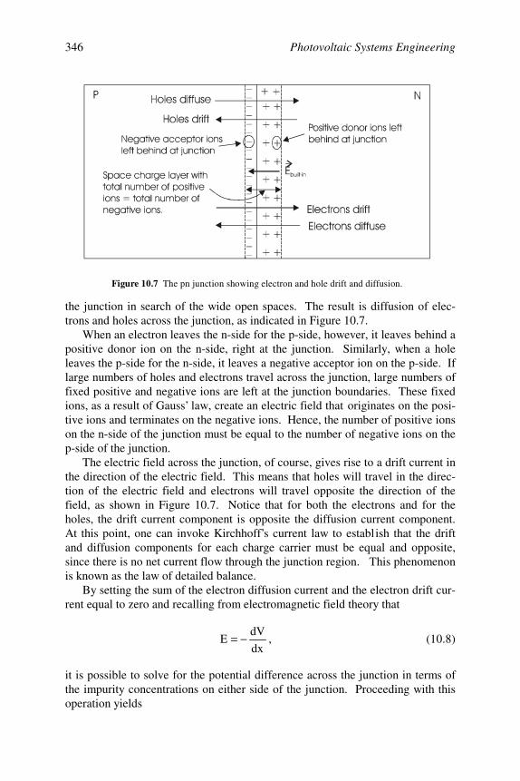
Photovoltaic Systems Engineering346
the junction in search of the wide open spaces. The result is diffusion of elec-trons and holes across the junction, as indicated in Figure 10.7.
When an electron leaves the n-side for the p-side, however, it leaves behind apositive donor ion on the n-side, right at the junction. Similarly, when a holeleaves the p-side for the n-side, it leaves a negative acceptor ion on the p-side. Iflarge numbers of holes and electrons travel across the junction, large numbers offixed positive and negative ions are left at the junction boundaries. These fixedions, as a result of Gauss’ law, create an electric field that originates on the posi-tive ions and terminates on the negative ions. Hence, the number of positive ionson the n-side of the junction must be equal to the number of negative ions on thep-side of the junction.
The electric field across the junction, of course, gives rise to a drift current inthe direction of the electric field. This means that holes will travel in the direc-tion of the electric field and electrons will travel opposite the direction of thefield, as shown in Figure 10.7. Notice that for both the electrons and for theholes, the drift current component is opposite the diffusion current component.At this point, one can invoke Kirchhoff’s current law to establish that the driftand diffusion components for each charge carrier must be equal and opposite,since there is no net current flow through the junction region. This phenomenonis known as the law of detailed balance.
By setting the sum of the electron diffusion current and the electron drift cur-rent equal to zero and recalling from electromagnetic field theory that
dx
dVE −= , (10.8)
it is possible to solve for the potential difference across the junction in terms ofthe impurity concentrations on either side of the junction. Proceeding with thisoperation yields
Figure 10.7 The pn junction showing electron and hole drift and diffusion.
Chapter 10 The Physics of Photovoltaic Cells 347
0dxdn
qDdxdV
nq nn =+µ− , (10.9a)
that can be rewritten as
ndnD
dVn
n
µ= . (10.9b)
Finally, recognizing the Einstein relationship, Dn/µ n = kT/q, which is discussedin solid state physics textbooks, and integrating both sides from the n-side of thejunction to the p-side of the junction, yields the magnitude of the built-in voltageacross the junction to be
po
noj n
nln
qkT
V = . (10.10a)
It is now possible to express the built-in potential in terms of the impurityconcentrations on either side of the junction by recognizing that nno ≅ ND andnpo ≅ (ni)
2/NA. Substituting these values into (10.10a) yields, finally,
2i
DAj
n
NNln
qkT
V = . (10.10b)
At this point, a word about the region containing the donor ions and acceptorions is in order. Note first that outside this region, electron and hole concentra-tions remain at their thermal equilibrium values. Within the region, however, theconcentration of electrons must change from the high value on the n-side to thelow value on the p-side. Similarly, the hole concentration must change from thehigh value on the p-side to the low value on the n-side. Considering that the highvalues are really high, i.e., on the order of 1018/cm3, while the low values arereally low, i.e., on the order of 102/cm3, this means that within a short distance ofthe beginning of the ionized region, the concentration must drop to significantlybelow the equilibrium value. Because the concentrations of charge carriers inthe ionized region are so low, this region is often termed the depletion region, inrecognition of the depletion of mobile charge carriers in the region. Further-more, because of the charge due to the ions in this region, the depletion region isalso often referred to as the space charge layer. For the balance of this text, thisregion will simply be referred to as the junction.
The next step in the development of the behavior of the pn junction in thepresence of sunlight is to let the sun shine in and see what happens.
The Illuminated pn JunctionEquation (10.3) governs the absorption of photons at or near a pn junction.
Noting that an absorbed photon releases an EHP, it is now possible to explorewhat happens after the generation of the EHP. Those EHPs generated within thepn junction will be considered first, followed by the EHPs generated outside, butnear, the junction.
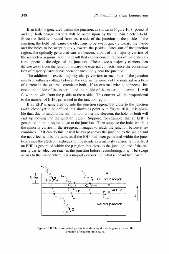
Photovoltaic Systems Engineering348
If an EHP is generated within the junction, as shown in Figure 10.8 (points Band C), both charge carriers will be acted upon by the built-in electric field.Since the field is directed from the n-side of the junction to the p-side of thejunction, the field will cause the electrons to be swept quickly toward the n-sideand the holes to be swept quickly toward the p-side. Once out of the junctionregion, the optically generated carriers become a part of the majority carriers ofthe respective regions, with the result that excess concentrations of majority car-riers appear at the edges of the junction. These excess majority carriers thendiffuse away from the junction toward the external contacts, since the concentra-tion of majority carriers has been enhanced only near the junction.
The addition of excess majority charge carriers to each side of the junctionresults in either a voltage between the external terminals of the material or a flowof current in the external circuit or both. If an external wire is connected be-tween the n-side of the material and the p-side of the material, a current, I
O, will
flow in the wire from the p-side to the n-side. This current will be proportionalto the number of EHPs generated in the junction region
If an EHP is generated outside the junction region, but close to the junction(with “close” yet to be defined, but shown as point A in Figure 10.8), it is possi-ble that, due to random thermal motion, either the electron, the hole, or both willend up moving into the junction region. Suppose, for example, that an EHP isgenerated in the n-region close to the junction. Then suppose the hole, which isthe minority carrier in the n-region, manages to reach the junction before it re-combines. If it can do this, it will be swept across the junction to the p-side andthe net effect will be the same as if the EHP had been generated within the junc-tion, since the electron is already on the n-side as a majority carrier. Similarly, ifan EHP is generated within the p-region, but close to the junction, and if the mi-nority carrier electron reaches the junction before recombining, it will be sweptacross to the n-side where it is a majority carrier. So what is meant by close?
,
-XQFWLRQ
(+3
(+3
(+3
1HXWUDOSUHJLRQ
1HXWUDOQUHJLRQB
BB
j
j
j
j(+3
α K ν
KνK ν
K ν
$
%&
'
Figure 10.8 The illuminated pn junction showing desirable geometry and thecreation of electron-hole pairs.
Chapter 10 The Physics of Photovoltaic Cells 349
Clearly, the minority carriers of the optically generated EHPs outside thejunction region must not recombine before they reach the junction. If they do,then, effectively, both carriers are lost from the conduction process, as in point Din Figure 10.8. Since the majority carrier is already on the correct side of thejunction, the minority carrier must therefore reach the junction in less than a mi-nority carrier lifetime, τ n or τ p.
To convert these times into distances, it is necessary to note that the carrierstravel by diffusion once they are created. Since only the thermal velocity hasbeen associated with diffusion, but since the thermal velocity is random in direc-tion, it is necessary to introduce the concept of minority carrier diffusion length,which represents the distance, on the average, which a minority carrier will travelbefore it recombines. The diffusion length can be shown to be related to theminority carrier lifetime and diffusion constant by the formula
mmm DL τ= , (10.11)
where m has been introduced to represent n for electrons or p for holes. It canalso be shown that on the average, if an EHP is generated within a minority car-rier diffusion length of the junction, the associated minority carrier will reach thejunction. In reality, some minority carriers generated closer than a diffusionlength will recombine before reaching the junction, while some minority carriersgenerated farther than a diffusion length from the junction will reach the junctionbefore recombining.
Hence, to maximize photocurrent, it is desirable to maximize the number ofphotons that will be absorbed either in the junction or within a minority carrierdiffusion length of the junction. The minority carriers of the EHPs generatedoutside this region have a higher probability of recombining before they have achance to diffuse to the junction. If a minority carrier from an optically gener-ated EHP recombines before it crosses the junction and becomes a majority car-rier, it, along with the opposite carrier with which it recombines, is no longeravailable for conduction. Furthermore, the combined width of the junction andthe two diffusion lengths should be several multiples of the reciprocal of the ab-sorption constant, α , and the junction should be relatively close to a diffusionlength from the surface of the material upon which the photon impinges, tomaximize collection of photons. Figure 10.8 shows this desirable geometry.The engineering design challenge then lies in maximizing α , as well as maxi-mizing the junction width and minority carrier diffusion lengths.
The Externally Biased pn JunctionIn order to complete the analysis of the theoretical performance of the pn
junction operating as a photovoltaic cell, it is useful to look at the junction withexternal bias. Figure 10.9 shows a pn junction connected to an external batterywith the internally generated electric field direction included. If (10.10a) is re-called, taking into account that the externally applied voltage, with the exception
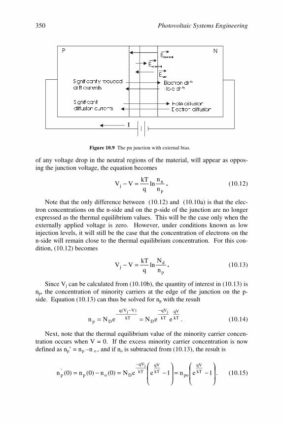
Photovoltaic Systems Engineering350
of any voltage drop in the neutral regions of the material, will appear as oppos-ing the junction voltage, the equation becomes
p
nj n
nln
qkT
VV =− . (10.12)
Note that the only difference between (10.12) and (10.10a) is that the elec-tron concentrations on the n-side and on the p-side of the junction are no longerexpressed as the thermal equilibrium values. This will be the case only when theexternally applied voltage is zero. However, under conditions known as lowinjection levels, it will still be the case that the concentration of electrons on then-side will remain close to the thermal equilibrium concentration. For this con-dition, (10.12) becomes
p
dj n
Nln
qkT
VV =− . (10.13)
Since Vj can be calculated from (10.10b), the quantity of interest in (10.13) isnp, the concentration of minority carriers at the edge of the junction on the p-side. Equation (10.13) can thus be solved for np with the result
kT
qV
kT
qV
DkT
)VV(q
Dp eeNeNnjj −−
−== . (10.14)
Next, note that the thermal equilibrium value of the minority carrier concen-tration occurs when V = 0. If the excess minority carrier concentration is nowdefined as np’ = np – n o , and if no is subtracted from (10.13), the result is
−=
−=−=
−
1en1eeN)0(n)0(n)0(n kT
qV
pokT
qV
kT
qV
Dop’p
j
. (10.15)
LQWHUQDO
QHW
H[WHUQDO
(OHFWURQGULIW+ROHGULIW
6LJQLILFDQWO\UHGXFHGGULIWFXUUHQWV
6LJQLILFDQWGLIIXVLRQFXUUHQWV
+ROHGLIIXVLRQ(OHFWURQGLIIXVLRQ
Figure 10.9 The pn junction with external bias.
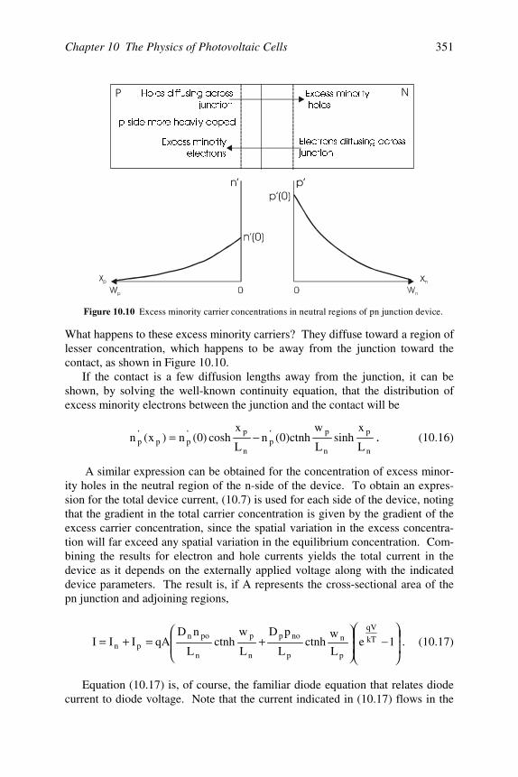
Chapter 10 The Physics of Photovoltaic Cells 351
What happens to these excess minority carriers? They diffuse toward a region oflesser concentration, which happens to be away from the junction toward thecontact, as shown in Figure 10.10.
If the contact is a few diffusion lengths away from the junction, it can beshown, by solving the well-known continuity equation, that the distribution ofexcess minority electrons between the junction and the contact will be
n
p
n
p’p
n
p’pp
’p L
xsinh
L
wctnh)0(n
L
xcosh)0(n)x(n −= . (10.16)
A similar expression can be obtained for the concentration of excess minor-ity holes in the neutral region of the n-side of the device. To obtain an expres-sion for the total device current, (10.7) is used for each side of the device, notingthat the gradient in the total carrier concentration is given by the gradient of theexcess carrier concentration, since the spatial variation in the excess concentra-tion will far exceed any spatial variation in the equilibrium concentration. Com-bining the results for electron and hole currents yields the total current in thedevice as it depends on the externally applied voltage along with the indicateddevice parameters. The result is, if A represents the cross-sectional area of thepn junction and adjoining regions,
−
+=+= 1e
L
wctnh
L
pD
L
wctnh
L
nDqAIII kT
qV
p
n
p
nop
n
p
n
ponpn . (10.17)
Equation (10.17) is, of course, the familiar diode equation that relates diodecurrent to diode voltage. Note that the current indicated in (10.17) flows in the
Figure 10.10 Excess minority carrier concentrations in neutral regions of pn junction device.
+ROHVGLIIXVLQJDFURVV
MXQFWLRQ([FHVVPLQRULW\
KROHV
(OHFWURQVGLIIXVLQJDFURVV
MXQFWLRQ
SVLGHPRUHKHDYLO\GRSHG
([FHVVPLQRULW\
HOHFWURQV
Photovoltaic Systems Engineering352
direction opposite to the optically generated current described earlier. LettingqA(nasty expression) = Io and incorporating the photocurrent component into(10.17) finally yields the complete equation for the current in the PV cell to be
−−= 1eIII kT
qV
ol. (10.18)
Those readers who remember everything they read will recognize (10.18) tobe the same as (3.1). Note that the current of (10.18) is directed out of the posi-tive terminal of the device, so that when the current and voltage are both posi-tive, the device is delivering power to the external circuit.
10.4 Maximizing PV Cell Performance
10.4.1 Introduction
Equation (10.18) indicates, albeit in a somewhat subtle manner, that tomaximize the power output of a PV cell, it is desirable to maximize the open-circuit voltage, short-circuit current, and fill factor of a cell. Recalling the plotof (10.18) from Chapter 3, it should be evident that maximizing the open-circuitvoltage and the short-circuit current will maximize the power output for an idealcell characterized by (10.18). Real cells, of course, have some series resistance,so there will be power dissipated by this resistance, similar to the power loss in aconventional battery due to its internal resistance. In any case, recalling that theopen-circuit voltage increases as the ratio of photo current to reverse saturationcurrent increases, a desirable design criteria is to maximize this ratio, providedthat it does not proportionally reduce the short-circuit current of the device.
Fortunately, this is not the case, since maximizing the short-circuit currentrequires maximizing the photocurrent. It is thus instructive to look closely at theparameters that determine both the reverse saturation current and the photocur-rent. Techniques for lowering series resistance will then be discussed.
10.4.2 Minimizing the Reverse Saturation Current
Beginning with the reverse saturation current as expressed in (10.17), thefirst observation is that the equilibrium minority carrier concentrations at theedges of the pn junction are related to the intrinsic carrier concentration through(10.4). Hence,
D
2i
no N
np = and
A
2i
po N
nn = . (10.19)
So far, no analytic expression for the intrinsic carrier concentration has beendeveloped. Such an expression can be obtained by considering Fermi levels,
Chapter 10 The Physics of Photovoltaic Cells 353
densities of states, and other quantities that are discussed in solid-state devicestextbooks. Since the goal here is to determine how to minimize the reverse satu-ration current, and not to go into detail of quantum mechanical proofs, the resultis noted here with the recommendation that the interested reader consult a goodsolid-state devices text for the development of the result. The result is
( ) kT
E*p
*n
3
22i
g
23
emmh
kT24n
−
π= , (10.20)
where mn* and mp
* are the electron effective mass and hole effective mass in thehost material and Eg is the bandgap energy of the host material. These effectivemasses can be greater than or less than the rest mass of the electron, dependingon the degree of curvature of the valence and conduction bands when plotted asenergy vs. momentum as in Figure 10.2. In fact, the effective mass can also de-pend on the band in which the carrier resides in a material. For more informa-tion on effective mass, the reader is encouraged to consult the references listed atthe end of the chapter.
Now, using (10.11) with (10.19) and (10.20) in (10.17) the following finalresult for the reverse saturation current is obtained.
( ) ×
π=
−kT
E
2
3*p
*n2o
g
emmh
kT2qA4I
ττ+
ττpp
n
p
p
Dnn
p
n
n
A Dctnh
D
N
1
Dctnh
D
N
1 . (10.21)
Since the design goal is to minimize Io while still maximizing the ratio Il:Io,
the next step is to express the photocurrent in some detail so the values of appro-priate parameters can be considered in the design choices.
10.4.3 Optimizing Photocurrent
In Section 10.3.2, the photocurrent optimization process was discussedqualitatively. In this section the specific parameters that govern the absorptionof light and the lifetime of the absorbed charge carriers will be discussed, and aformula for the photocurrent will be presented for comparison with the formulafor reverse saturation current. In particular, minimizing reflection of the incidentphotons, maximizing the minority carrier diffusion lengths, maximizing thejunction width and minimizing surface recombination velocity will be discussed.The PV cell designer will then know exactly what to do to make the perfect cell.
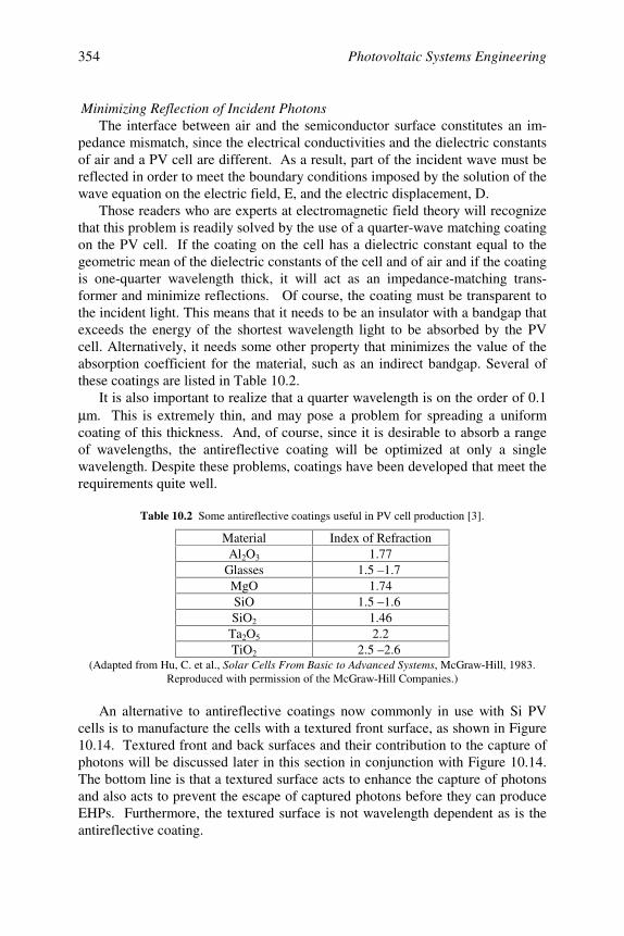
Photovoltaic Systems Engineering354
Minimizing Reflection of Incident PhotonsThe interface between air and the semiconductor surface constitutes an im-
pedance mismatch, since the electrical conductivities and the dielectric constantsof air and a PV cell are different. As a result, part of the incident wave must bereflected in order to meet the boundary conditions imposed by the solution of thewave equation on the electric field, E, and the electric displacement, D.
Those readers who are experts at electromagnetic field theory will recognizethat this problem is readily solved by the use of a quarter-wave matching coatingon the PV cell. If the coating on the cell has a dielectric constant equal to thegeometric mean of the dielectric constants of the cell and of air and if the coatingis one-quarter wavelength thick, it will act as an impedance-matching trans-former and minimize reflections. Of course, the coating must be transparent tothe incident light. This means that it needs to be an insulator with a bandgap thatexceeds the energy of the shortest wavelength light to be absorbed by the PVcell. Alternatively, it needs some other property that minimizes the value of theabsorption coefficient for the material, such as an indirect bandgap. Several ofthese coatings are listed in Table 10.2.
It is also important to realize that a quarter wavelength is on the order of 0.1µ m. This is extremely thin, and may pose a problem for spreading a uniformcoating of this thickness. And, of course, since it is desirable to absorb a rangeof wavelengths, the antireflective coating will be optimized at only a singlewavelength. Despite these problems, coatings have been developed that meet therequirements quite well.
Table 10.2 Some antireflective coatings useful in PV cell production [3].
Material Index of RefractionAl2O3 1.77
Glasses 1.5 – 1.7MgO 1.74SiO 1.5 – 1.6SiO2 1.46
Ta2O5 2.2TiO2 2.5 – 2.6
(Adapted from Hu, C. et al., Solar Cells From Basic to Advanced Systems, McGraw-Hill, 1983.Reproduced with permission of the McGraw-Hill Companies.)
An alternative to antireflective coatings now commonly in use with Si PVcells is to manufacture the cells with a textured front surface, as shown in Figure10.14. Textured front and back surfaces and their contribution to the capture ofphotons will be discussed later in this section in conjunction with Figure 10.14.The bottom line is that a textured surface acts to enhance the capture of photonsand also acts to prevent the escape of captured photons before they can produceEHPs. Furthermore, the textured surface is not wavelength dependent as is theantireflective coating.
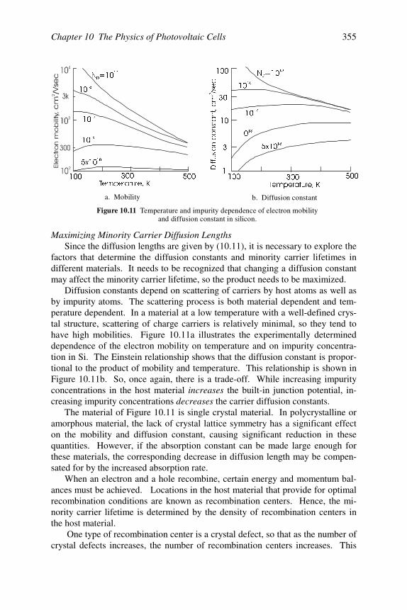
Chapter 10 The Physics of Photovoltaic Cells 355
Maximizing Minority Carrier Diffusion LengthsSince the diffusion lengths are given by (10.11), it is necessary to explore the
factors that determine the diffusion constants and minority carrier lifetimes indifferent materials. It needs to be recognized that changing a diffusion constantmay affect the minority carrier lifetime, so the product needs to be maximized.
Diffusion constants depend on scattering of carriers by host atoms as well asby impurity atoms. The scattering process is both material dependent and tem-perature dependent. In a material at a low temperature with a well-defined crys-tal structure, scattering of charge carriers is relatively minimal, so they tend tohave high mobilities. Figure 10.11a illustrates the experimentally determineddependence of the electron mobility on temperature and on impurity concentra-tion in Si. The Einstein relationship shows that the diffusion constant is propor-tional to the product of mobility and temperature. This relationship is shown inFigure 10.11b. So, once again, there is a trade-off. While increasing impurityconcentrations in the host material increases the built-in junction potential, in-creasing impurity concentrations decreases the carrier diffusion constants.
The material of Figure 10.11 is single crystal material. In polycrystalline oramorphous material, the lack of crystal lattice symmetry has a significant effecton the mobility and diffusion constant, causing significant reduction in thesequantities. However, if the absorption constant can be made large enough forthese materials, the corresponding decrease in diffusion length may be compen-sated for by the increased absorption rate.
When an electron and a hole recombine, certain energy and momentum bal-ances must be achieved. Locations in the host material that provide for optimalrecombination conditions are known as recombination centers. Hence, the mi-nority carrier lifetime is determined by the density of recombination centers inthe host material.
One type of recombination center is a crystal defect, so that as the number ofcrystal defects increases, the number of recombination centers increases. This
7HPSHUDWXUH.
1 '
1 '
7HPSHUDWXUH.
'LIIXVLRQFRQVWDQWFPVHF
[
[
Figure 10.11 Temperature and impurity dependence of electron mobilityand diffusion constant in silicon.
a. Mobility b. Diffusion constant
Photovoltaic Systems Engineering356
means that crystal defects reduce the diffusion constant as well as the minoritycarrier lifetime in a material.
Impurities also generally make good recombination centers, especially thoseimpurities with energies near the center of the bandgap. These impurities arethus different from the donor and acceptor impurities that are purposefully usedin the host material, since donor impurities have energies relatively close to theconduction band and acceptor impurities have energies relatively close to thevalence band.
Minority carrier lifetimes also depend on the concentration of charge carriersin the material. An approximation of the dependence of electron minority carrierlifetime on carrier concentration and location of the trapping energy within theenergy gap is given by
)nnp(CN
kT
EEcoshn2pnn
2it
iti
’
n −
−
++=τ , (10.22a)
where C is the capture cross section of the impurity in cm3/sec, Nt is the den-sity of trapping centers and Et and Ei are the energies of the trapping centerand the intrinsic Fermi level. In most materials, the intrinsic Fermi level is veryclose to the center of the bandgap. Under most illumination conditions, the hy-perbolic term will be negligible compared to the majority carrier concentrationand the excess electron concentration as minority carriers in p-type material willbe much larger than the electron thermal equilibrium concentration. Under theseconditions, for minority electrons in p-type material, (10.22a) reduces to
tn CN
1≅τ . (10.22b)
Hence, to maximize the minority carrier lifetime, it is necessary to minimize theconcentration of trapping centers and to be sure that any existing trapping cen-ters have minimal capture cross sections.
Maximizing Junction WidthSince it has been determined that it is desirable to absorb photons within the
confines of the pn junction, it is desirable to maximize the width of the junction.It is therefore necessary to explore the parameters that govern the junction width.Perhaps the reader recalls similar discussions in a previous electronics class.
An expression for the width of a pn junction can be obtained by solvingGauss’ law at the junction, since the junction is a region that contains electriccharge. Solution of Gauss’ law, of course, is dependent upon the ability to ex-press the spatial distribution of the space charge in mathematical, or, at least, ingraphical form. Depending on the process used to form the junction, the impu-rity profile across the junction can be approximated by different expressions.Junctions formed by epitaxial growth or by ion implantation can be controlled to
Chapter 10 The Physics of Photovoltaic Cells 357
have impurity profiles to meet the discretion of the operator. Junctions grown bydiffusion can be reasonably approximated by a linearly graded model. The in-terested reader is encouraged to consult a reference on semiconductor devicesfor detailed information on the production of various junction impurity profiles.
The junction with uniform concentrations of impurities is convenient to useto obtain a feeling for how to maximize the width of a junction. Solution ofGauss’ law for a junction with uniform concentration of donors on one side and auniform concentration of acceptors on the other side yields solutions for thewidth of the space charge layer on each side of the junction. The total junctionwidth is then simply the sum of the widths of the two sides of the space chargelayer. The results for each side are
( ) 212
1
VV)NN(qN
N2W j
DAD
An −
+
ε= (10.23a)
and
( ) 212
1
VV)NN(qN
N2W j
ADA
Dp −
+
ε= . (10.23b)
Before combining these two results, it is interesting to note that the width ofthe junction on either the p-side or on the n-side depends on the ratio of the im-purity concentrations on each side. Again, since Gauss’ law requires equal num-bers of charges on each side of the junction, the side with the smaller impurityconcentration will need to have a wider space charge layer to produce enoughimpurity ions to balance out the impurity ions on the other side. The overallwidth of the junction can now be determined by summing equations (10.23a) and(10.23b) to get
( ) 212
1
VVNqN
)NN(2W j
DA
AD −
+ε= . (10.24)
At this point, it should be recognized that the voltage across the junction dueto the external voltage across the cell, V, will never exceed the built-in voltage,Vj. The reason is that, as the externally applied voltage becomes more positive,the cell current increases exponentially and causes voltage drops in the neutralregions of the cell, so only a fraction of the externally applied voltage actuallyappears across the junction. Hence, there is no need to worry about the junctionwidth becoming zero or imaginary. In the case of photovoltaic operation, theexternal cell voltage will hopefully be at the maximum power point, which isgenerally between 0.5 V and 0.6 V for silicon.
Next, observe that, as the external cell voltage increases, the width of thejunction decreases. As a result, the absorption of photons decreases. This sug-
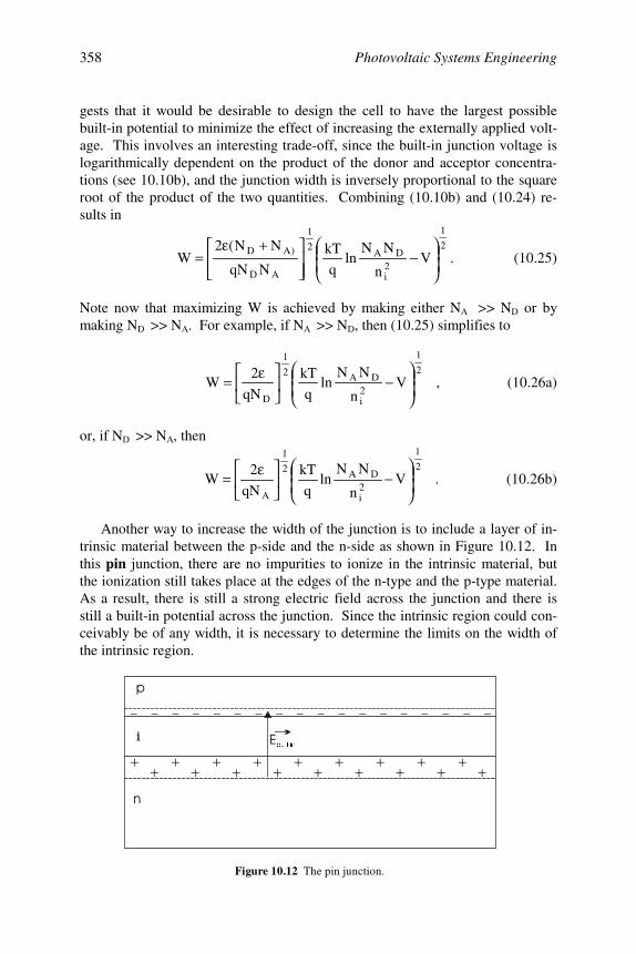
Photovoltaic Systems Engineering358
gests that it would be desirable to design the cell to have the largest possiblebuilt-in potential to minimize the effect of increasing the externally applied volt-age. This involves an interesting trade-off, since the built-in junction voltage islogarithmically dependent on the product of the donor and acceptor concentra-tions (see 10.10b), and the junction width is inversely proportional to the squareroot of the product of the two quantities. Combining (10.10b) and (10.24) re-sults in
2
1
2i
DA2
1
AD
)ADV
n
NNln
q
kT
NqN
NN(2W
−
+ε= . (10.25)
Note now that maximizing W is achieved by making either NA >> ND or bymaking ND >> NA. For example, if NA >> ND, then (10.25) simplifies to
2
1
2i
DA2
1
D
Vn
NNln
q
kT
qN
2W
−
ε= , (10.26a)
or, if ND >> NA, then
2
1
2i
DA2
1
A
Vn
NNln
q
kT
qN
2W
−
ε= . (10.26b)
Another way to increase the width of the junction is to include a layer of in-trinsic material between the p-side and the n-side as shown in Figure 10.12. Inthis pin junction, there are no impurities to ionize in the intrinsic material, butthe ionization still takes place at the edges of the n-type and the p-type material.As a result, there is still a strong electric field across the junction and there isstill a built-in potential across the junction. Since the intrinsic region could con-ceivably be of any width, it is necessary to determine the limits on the width ofthe intrinsic region.
i EXLOWLQ
Figure 10.12 The pin junction.
Chapter 10 The Physics of Photovoltaic Cells 359
The only feature of the intrinsic region that degrades performance is the factthat it has a width. If it has a width, then it takes time for a charge carrier to tra-verse this width. If it takes time, then there is a chance that the carrier will re-combine. Thus, the width of the intrinsic layer simply needs to be kept shortenough to minimize recombination. The particles travel through the intrinsicregion with a relatively high drift velocity due to the built-in electric field at thejunction. Since the thermal velocities of the carriers still exceed the drift veloci-ties by several orders of magnitude, the width of the intrinsic layer needs to bekept on the order of about one diffusion length.
Minimizing Surface Recombination VelocityIf an EHP is generated near a surface, it becomes more probable that the mi-
nority carrier will diffuse to the surface. Since photocurrent depends on minoritycarriers’ diffusing to the junction and ultimately across the junction, surface re-combination of minority carriers before they can travel to the junction reducesthe available photocurrent. When the surface is within a minority carrier diffu-sion length of the junction, which is often desirable to ensure that generation ofEHPs is maximized near the junction, minority carrier surface recombination cansignificantly reduce the efficiency of the cell.
Surface recombination depends on the density of excess minority carriers, inthis case, as generated by photon absorption, and on the average recombinationcenter density per unit area, Nsr, on the surface. The density of recombinationcenters is very high at contacts and is also high at surfaces in general, since thecrystal structure is interrupted at the surface. Imperfections at the surface,whether due to impurities or to crystal defects, all act as recombination centers.
The recombination rate, U, is expressed as number/cm2/sec and is given by
U = cNsrm', (10.27)
where m' is used to represent the excess minority carrier concentration, whetherelectrons or holes, and c is a constant that incorporates the lifetime of a minoritycarrier at a recombination center. Analysis of the dimensions of the parametersin (10.27) shows that the units of cNsr are cm/sec. This product is called the sur-face recombination velocity, S. The total number of excess minority carriersrecombining per unit time and subsequent loss of potential photocurrent, is thusdependent on the density of recombination centers at the surface and on the areaof the surface. Minimizing surface recombination thus may involve reducing thedensity of recombination centers or reducing the density of minority carriers atthe surface.
If the surface is completely covered by a contact, then little can be done toreduce surface recombination if minority carriers reach the surface, since recom-bination rates at contacts are very high. However, if the surface is not com-pletely covered by a contact, such as at the front surface, then a number of tech-niques have been discovered that will result in passivation of the surface. Silicon
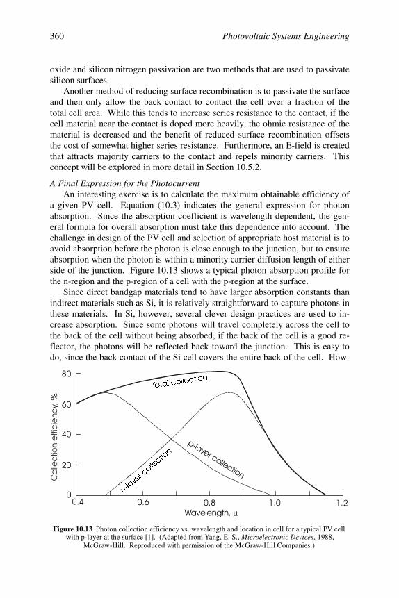
Photovoltaic Systems Engineering360
oxide and silicon nitrogen passivation are two methods that are used to passivatesilicon surfaces.
Another method of reducing surface recombination is to passivate the surfaceand then only allow the back contact to contact the cell over a fraction of thetotal cell area. While this tends to increase series resistance to the contact, if thecell material near the contact is doped more heavily, the ohmic resistance of thematerial is decreased and the benefit of reduced surface recombination offsetsthe cost of somewhat higher series resistance. Furthermore, an E-field is createdthat attracts majority carriers to the contact and repels minority carriers. Thisconcept will be explored in more detail in Section 10.5.2.
A Final Expression for the PhotocurrentAn interesting exercise is to calculate the maximum obtainable efficiency of
a given PV cell. Equation (10.3) indicates the general expression for photonabsorption. Since the absorption coefficient is wavelength dependent, the gen-eral formula for overall absorption must take this dependence into account. Thechallenge in design of the PV cell and selection of appropriate host material is toavoid absorption before the photon is close enough to the junction, but to ensureabsorption when the photon is within a minority carrier diffusion length of eitherside of the junction. Figure 10.13 shows a typical photon absorption profile forthe n-region and the p-region of a cell with the p-region at the surface.
Since direct bandgap materials tend to have larger absorption constants thanindirect materials such as Si, it is relatively straightforward to capture photons inthese materials. In Si, however, several clever design practices are used to in-crease absorption. Since some photons will travel completely across the cell tothe back of the cell without being absorbed, if the back of the cell is a good re-flector, the photons will be reflected back toward the junction. This is easy todo, since the back contact of the Si cell covers the entire back of the cell. How-
µ
7RWDOFROOHFWLRQ
QOD\HUF
ROOHFWLRQ
Figure 10.13 Photon collection efficiency vs. wavelength and location in cell for a typical PV cell with p-layer at the surface [1]. (Adapted from Yang, E. S., , 1988,
McGraw-Hill. Reproduced with permission of the McGraw-Hill Companies.)Microelectronic Devices
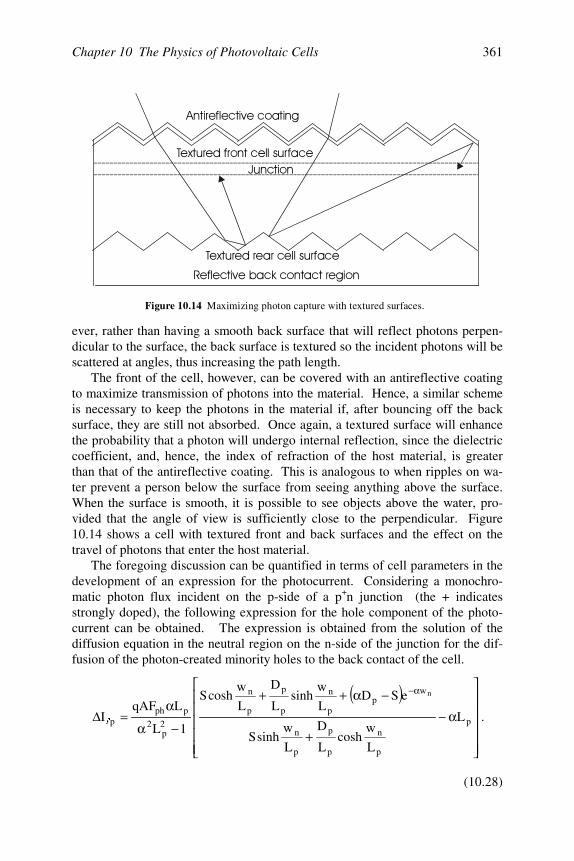
Chapter 10 The Physics of Photovoltaic Cells 361
ever, rather than having a smooth back surface that will reflect photons perpen-dicular to the surface, the back surface is textured so the incident photons will bescattered at angles, thus increasing the path length.
The front of the cell, however, can be covered with an antireflective coatingto maximize transmission of photons into the material. Hence, a similar schemeis necessary to keep the photons in the material if, after bouncing off the backsurface, they are still not absorbed. Once again, a textured surface will enhancethe probability that a photon will undergo internal reflection, since the dielectriccoefficient, and, hence, the index of refraction of the host material, is greaterthan that of the antireflective coating. This is analogous to when ripples on wa-ter prevent a person below the surface from seeing anything above the surface.When the surface is smooth, it is possible to see objects above the water, pro-vided that the angle of view is sufficiently close to the perpendicular. Figure10.14 shows a cell with textured front and back surfaces and the effect on thetravel of photons that enter the host material.
The foregoing discussion can be quantified in terms of cell parameters in thedevelopment of an expression for the photocurrent. Considering a monochro-matic photon flux incident on the p-side of a p+n junction (the + indicatesstrongly doped), the following expression for the hole component of the photo-current can be obtained. The expression is obtained from the solution of thediffusion equation in the neutral region on the n-side of the junction for the dif-fusion of the photon-created minority holes to the back contact of the cell.
( )
α−+
−α++
−α
α=∆
α−
p
p
n
p
p
p
n
wp
p
n
p
p
p
n
2p
2
pphp L
L
wcosh
L
D
L
wsinhS
eSDL
wsinh
L
D
L
wcoshS
1L
LqAFI
n
l.
(10.28)
!"#$"
%
!"#$"&"
Figure 10.14 Maximizing photon capture with textured surfaces.
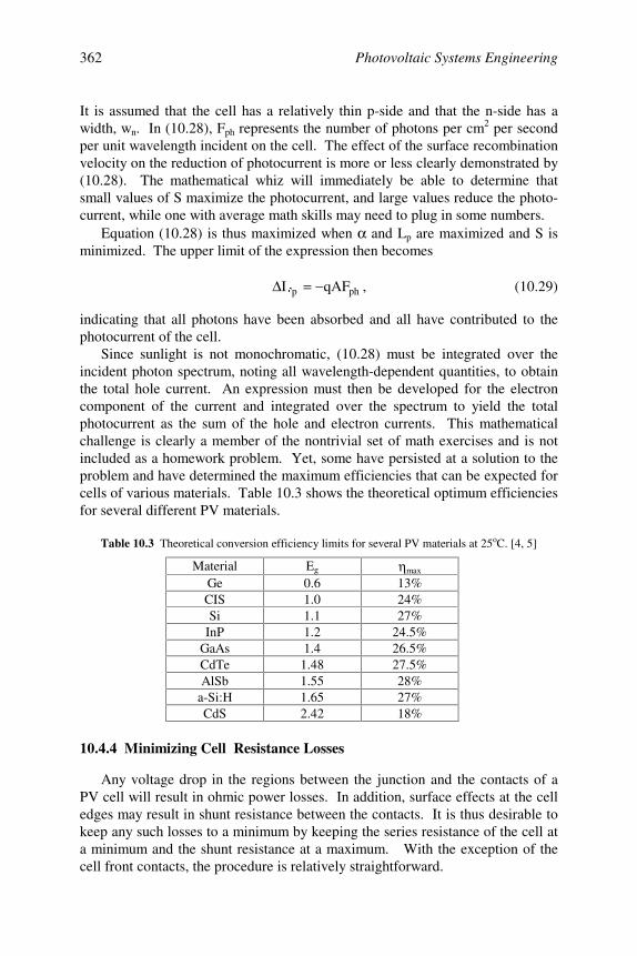
Photovoltaic Systems Engineering362
It is assumed that the cell has a relatively thin p-side and that the n-side has awidth, wn. In (10.28), Fph represents the number of photons per cm2 per secondper unit wavelength incident on the cell. The effect of the surface recombinationvelocity on the reduction of photocurrent is more or less clearly demonstrated by(10.28). The mathematical whiz will immediately be able to determine thatsmall values of S maximize the photocurrent, and large values reduce the photo-current, while one with average math skills may need to plug in some numbers.
Equation (10.28) is thus maximized when α and Lp are maximized and S isminimized. The upper limit of the expression then becomes
php qAFI −=∆l
, (10.29)
indicating that all photons have been absorbed and all have contributed to thephotocurrent of the cell.
Since sunlight is not monochromatic, (10.28) must be integrated over theincident photon spectrum, noting all wavelength-dependent quantities, to obtainthe total hole current. An expression must then be developed for the electroncomponent of the current and integrated over the spectrum to yield the totalphotocurrent as the sum of the hole and electron currents. This mathematicalchallenge is clearly a member of the nontrivial set of math exercises and is notincluded as a homework problem. Yet, some have persisted at a solution to theproblem and have determined the maximum efficiencies that can be expected forcells of various materials. Table 10.3 shows the theoretical optimum efficienciesfor several different PV materials.
Table 10.3 Theoretical conversion efficiency limits for several PV materials at 25oC. [4, 5]
Material Eg η max
Ge 0.6 13%CIS 1.0 24%Si 1.1 27%
InP 1.2 24.5%GaAs 1.4 26.5%CdTe 1.48 27.5%AlSb 1.55 28%
a-Si:H 1.65 27%CdS 2.42 18%
10.4.4 Minimizing Cell Resistance Losses
Any voltage drop in the regions between the junction and the contacts of aPV cell will result in ohmic power losses. In addition, surface effects at the celledges may result in shunt resistance between the contacts. It is thus desirable tokeep any such losses to a minimum by keeping the series resistance of the cell ata minimum and the shunt resistance at a maximum. With the exception of thecell front contacts, the procedure is relatively straightforward.
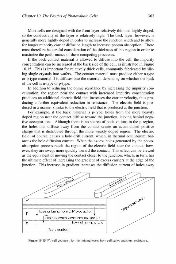
Chapter 10 The Physics of Photovoltaic Cells 363
Most cells are designed with the front layer relatively thin and highly doped,so the conductivity of the layer is relatively high. The back layer, however, isgenerally more lightly doped in order to increase the junction width and to allowfor longer minority carrier diffusion length to increase photon absorption. Theremust therefore be careful consideration of the thickness of this region in order tomaximize the performance of these competing processes.
If the back contact material is allowed to diffuse into the cell, the impurityconcentration can be increased at the back side of the cell, as illustrated in Figure10.15. This is important for relatively thick cells, commonly fabricated by slic-ing single crystals into wafers. The contact material must produce either n-typeor p-type material if it diffuses into the material, depending on whether the backof the cell is n-type or p-type.
In addition to reducing the ohmic resistance by increasing the impurity con-centration, the region near the contact with increased impurity concentrationproduces an additional electric field that increases the carrier velocity, thus pro-ducing a further equivalent reduction in resistance. The electric field is pro-duced in a manner similar to the electric field that is produced at the junction.
For example, if the back material is p-type, holes from the more heavilydoped region near the contact diffuse toward the junction, leaving behind nega-tive acceptor ions. Although there is no source of positive ions in the p-region,the holes that diffuse away from the contact create an accumulated positivecharge that is distributed through the more weakly doped region. The electricfield, of course, causes a hole drift current, which, in thermal equilibrium, bal-ances the hole diffusion current. When the excess holes generated by the photo-absorption process reach the region of the electric field near the contact, how-ever, they are swept more quickly toward the contact. This effect can be viewedas the equivalent of moving the contact closer to the junction, which, in turn, hasthe ultimate effect of increasing the gradient of excess carriers at the edge of thejunction. This increase in gradient increases the diffusion current of holes away
Q
S
S
%DFNFRQWDFW
+ROHVGLIIXVLQJIURP(+3SURGXFWLRQ
BBBBBBBBBBBB/D\HURIDFFHSWRULRQV
(IURPDFFHSWRUFRQFHQWUDWLRQJUDGLHQW
7RSFR
QWDFW
7RSFR
QWDFW
(GJHS
DVVLYD
WLRQ

Photovoltaic Systems Engineering364
from the junction. Since this diffusion current strongly dominates the total cur-rent, the total current across the junction is thus increased by the heavily dopedlayer near the back contact.
At the front contact, another balancing act is needed. Ideally, the front con-tact should cover the entire front surface. The problem with this, however, isthat if the front contact is not transparent to the incident photons, it will reflectthem away. In most cases, the front contact is reflecting. Since the front/toplayer of the cell is generally very thin, even though it may be heavily doped, theresistance in the transverse direction will be relatively high because of the thinlayer. This means that if the contact is placed at the edge of the cell to enablemaximum photon absorption, the resistance along the surface to the contact willbe relatively large.
The compromise, then, is to create a contact that covers the front surface withmany tiny fingers, as shown in Figure 10.15. This network of tiny fingers,which, in turn, are connected to larger and larger fingers, is similar to the con-figuration of the capillaries that feed veins in a circulatory system. The idea is tomaintain more or less constant current density in the contact fingers, so that asmore current is collected, the cross-sectional area of the contact must be in-creased. This subject is covered in more detail in the next chapter.
Finally, shunt resistance is maximized by ensuring that no leakage occurs atthe perimeter of the cell. This can be done by nitrogen passivation or simply bycoating the edge of the cell with insulating material to prevent contaminants fromproviding a current path across the junction at the edges.
10.5 Exotic Junctions
10.5.1 Introduction
Thus far, only relatively simple junctions have been considered. PV cellperformance can be enhanced significantly by incorporating a variety of moresophisticated junctions, including, but not necessarily limited to: graded junc-tions, heterojunctions, Schottky junctions, multijunctions and tunnel junctions.This section provides an introduction to these junctions so the reader will betterunderstand the various junction types in the specific devices to be presented inthe next chapter.
10.5.2 Graded Junctions
All the formulations to this point have related to the abrupt junction, in whichthe impurity concentration is constant to the junction and then abruptly changesto the opposite impurity concentration. While these junctions do exist, gradedjunctions are more common in materials for which the junction is fabricated bydiffusion of impurities from the surface. The fabrication process for obtaining alinearly graded impurity profile as shown in Figure 10.16 will be discussed insome detail in the next chapter.
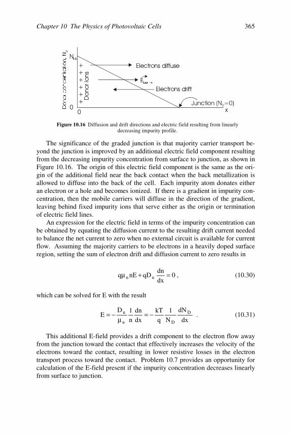
Chapter 10 The Physics of Photovoltaic Cells 365
The significance of the graded junction is that majority carrier transport be-yond the junction is improved by an additional electric field component resultingfrom the decreasing impurity concentration from surface to junction, as shown inFigure 10.16. The origin of this electric field component is the same as the ori-gin of the additional field near the back contact when the back metallization isallowed to diffuse into the back of the cell. Each impurity atom donates eitheran electron or a hole and becomes ionized. If there is a gradient in impurity con-centration, then the mobile carriers will diffuse in the direction of the gradient,leaving behind fixed impurity ions that serve either as the origin or terminationof electric field lines.
An expression for the electric field in terms of the impurity concentration canbe obtained by equating the diffusion current to the resulting drift current neededto balance the net current to zero when no external circuit is available for currentflow. Assuming the majority carriers to be electrons in a heavily doped surfaceregion, setting the sum of electron drift and diffusion current to zero results in
0dx
dnqDnEq nn =+µ , (10.30)
which can be solved for E with the result
dx
dN
N1
qkT
dxdn
n1D
E D
Dn
n −=µ
−= . (10.31)
This additional E-field provides a drift component to the electron flow awayfrom the junction toward the contact that effectively increases the velocity of theelectrons toward the contact, resulting in lower resistive losses in the electrontransport process toward the contact. Problem 10.7 provides an opportunity forcalculation of the E-field present if the impurity concentration decreases linearlyfrom surface to junction.
''6
!
(
$
$#"$
EXLOWLQ
$#
'RQRUFRQFHQWUDWLRQ1'
Figure 10.16 Diffusion and drift directions and electric field resulting from linearlydecreasing impurity profile.
Photovoltaic Systems Engineering366
10.5.3 Heterojunctions
One of the problems identified with the optical absorption process is the ab-sorption of higher energy photons close to the surface of the cell. Most of theEHPs generated by these higher energy photons are lost to recombination whenthey are created more than a diffusion length from the junction.
This phenomenon can be mitigated to some extent by the use of a hetero-junction. A heterojunction is simply a composite junction comprised of twomaterials with closely matched crystal lattices, so the bandgap near the surface ofthe material is greater than the bandgap near the junction. The higher bandgapregion will appear transparent to photons with lower energies, so these photonscan penetrate to the junction region where the bandgap is less than the incidentphoton energy. In the region of the junction, they can generate EHPs that will becollected before they recombine.
Heterojunctions are sometimes made between two n-regions or two p-regionsas well as between n-region and p-region. The behavior of the heterojunction isdependent upon the crystal lattices, work functions, impurity doping profiles andenergy band properties of each semiconductor material, to the extent that discus-sion of any particular junction would probably not be applicable to a differentjunction. Readers interested in specific junctions, such as Ge:GaAs or Al-GaAs:GaAs, will be able to obtain more information from journal and confer-ence publications.
In some cases, materials cannot be made either n-type or p-type. Use of aheterojunction with a material that can be made to complete a pn junction is an-other important use of heterojunctions. For example, p-type CdS is yet to beproduced. But a thin n-type CdS layer on top of a CIS structure will produce apn junction effect, so CdS is often used as a part of a thin film structure to pro-duce a thin, heavily doped n-region near the front surface of the cell.
10.5.4 Schottky Junctions
Sometimes, when a metal is contacted with semiconductor material, an ohmiccontact is formed and sometimes a rectifying contact is formed. It all dependson the relative positions of the work functions of the two materials. Figure 10.17shows situations where the work function of the metal, q φ m, is greater than thatof the n-type semiconductor, q φ s, and where the work function of the metal isless than that of the n-type semiconductor material. The work function is simplythe energy difference between the Fermi level and the vacuum level and theFermi level is that energy where the probability of occupancy by a mobile carrieris 0.5. For the semiconductor, the energy difference between the bottom of theconduction band and the vacuum level is designated as q ψ s.
When the metal and semiconductor are joined, electrons flow either frommetal to semiconductor or from semiconductor to metal, depending on which hasthe higher Fermi level. In the case where q φ s < q φ m, as indicated in Figure10.17a, electrons will flow from semiconductor to metal in a manner similar to
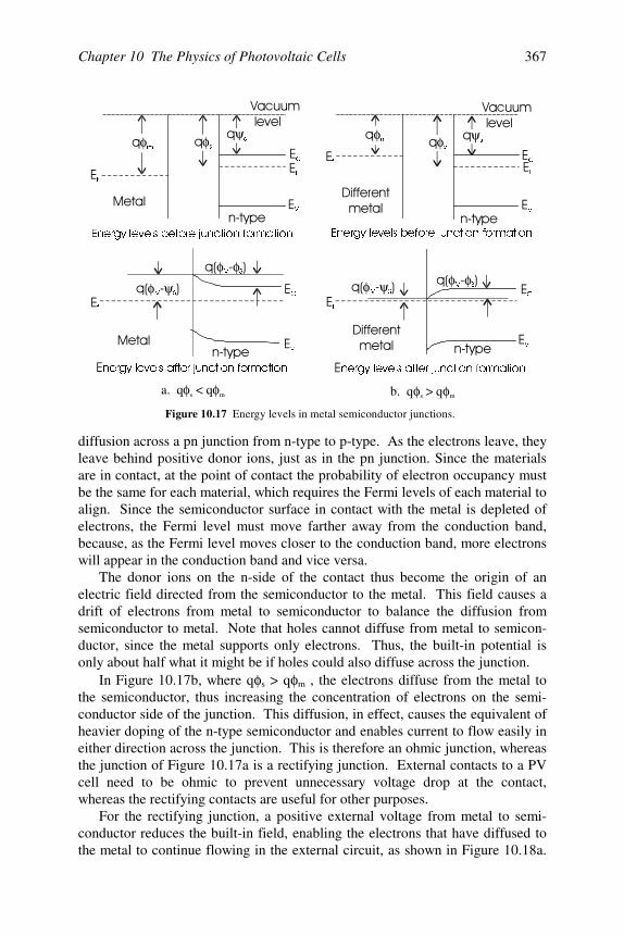
Chapter 10 The Physics of Photovoltaic Cells 367
diffusion across a pn junction from n-type to p-type. As the electrons leave, theyleave behind positive donor ions, just as in the pn junction. Since the materialsare in contact, at the point of contact the probability of electron occupancy mustbe the same for each material, which requires the Fermi levels of each material toalign. Since the semiconductor surface in contact with the metal is depleted ofelectrons, the Fermi level must move farther away from the conduction band,because, as the Fermi level moves closer to the conduction band, more electronswill appear in the conduction band and vice versa.
The donor ions on the n-side of the contact thus become the origin of anelectric field directed from the semiconductor to the metal. This field causes adrift of electrons from metal to semiconductor to balance the diffusion fromsemiconductor to metal. Note that holes cannot diffuse from metal to semicon-ductor, since the metal supports only electrons. Thus, the built-in potential isonly about half what it might be if holes could also diffuse across the junction.
In Figure 10.17b, where q φ s > q φ m , the electrons diffuse from the metal tothe semiconductor, thus increasing the concentration of electrons on the semi-conductor side of the junction. This diffusion, in effect, causes the equivalent ofheavier doping of the n-type semiconductor and enables current to flow easily ineither direction across the junction. This is therefore an ohmic junction, whereasthe junction of Figure 10.17a is a rectifying junction. External contacts to a PVcell need to be ohmic to prevent unnecessary voltage drop at the contact,whereas the rectifying contacts are useful for other purposes.
For the rectifying junction, a positive external voltage from metal to semi-conductor reduces the built-in field, enabling the electrons that have diffused tothe metal to continue flowing in the external circuit, as shown in Figure 10.18a.
)""*
)""*
+φP
φPφ
V φV
ψV ψ
V
&
&
9
9
I
I
I
I
(QHUJ\OHYHOVEHIRUHMXQFWLRQIRUPDWLRQ (QHUJ\OHYHOVEHIRUHMXQFWLRQIRUPDWLRQ
&
&
9
9
I
I
φ ψ0 6
φ ψ0 6
φ φ0 6
φ φ0 6
QHUJ\OHYHOVDIWHUMXQFWLRQIRUPDWLRQ QHUJ\OHYHOVDIWHUMXQFWLRQIRUPDWLRQ
a. q < qφ φs m b. q > qφ φs m
Figure 10.17 Energy levels in metal semiconductor junctions.
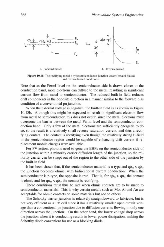
Photovoltaic Systems Engineering368
Note that as the Fermi level on the semiconductor side is drawn closer to theconduction band, more electrons can diffuse to the metal, resulting in significantcurrent flow from metal to semiconductor. The reduced built-in field reducesdrift components in the opposite direction in a manner similar to the forward biascondition of a conventional pn junction.
When the external voltage is negative, the built-in field is as shown in Figure10.18b. Although this might be expected to result in significant electron flowfrom metal to semiconductor, this does not occur, since the metal electrons mustovercome the barrier between the metal Fermi level and the semiconductor con-duction band. Only a few of the metal electrons are sufficiently energetic to doso, so the result is a relatively small reverse saturation current, and thus a recti-fying contact. The contact is rectifying even though the relatively strong E-fieldin the semiconductor region would be capable of enhancing drift current if re-placement mobile charges were available.
For PV action, photons need to generate EHPs on the semiconductor side ofthe junction within a minority carrier diffusion length of the junction, so the mi-nority carrier can be swept out of the region to the other side of the junction bythe built-in field.
It has been shown that, if the semiconductor material is n-type and q φ m < q φ s,the junction becomes ohmic, with bidirectional current conduction. When thesemiconductor is p-type, the opposite is true. That is, for q φ m > q φ s, the contactis ohmic and for q φ m < q φ s, the contact is rectifying.
These conditions must thus be met when ohmic contacts are to be made tosemiconductor materials. This is why certain metals such as Mo, Al and Au areacceptable for ohmic contacts on some materials but not on others.
The Schottky barrier junction is relatively straightforward to fabricate, but isnot very efficient as a PV cell since it has a relatively smaller open-circuit volt-age than a conventional pn junction due to diffusion currents flowing in only onedirection across the junction. On the other hand, the lower voltage drop acrossthe junction when it is conducting results in lower power dissipation, making theSchottky diode convenient for use as a blocking diode.
&
&
9
9
IP
IP
IV
IV
φ ψ0 6
φ ψ0 6
U
Figure 10.18 The rectifying metal-n-type semiconductor junction under forward biasedand reverse biased conditions.
a. Forward biased b. Reverse biased
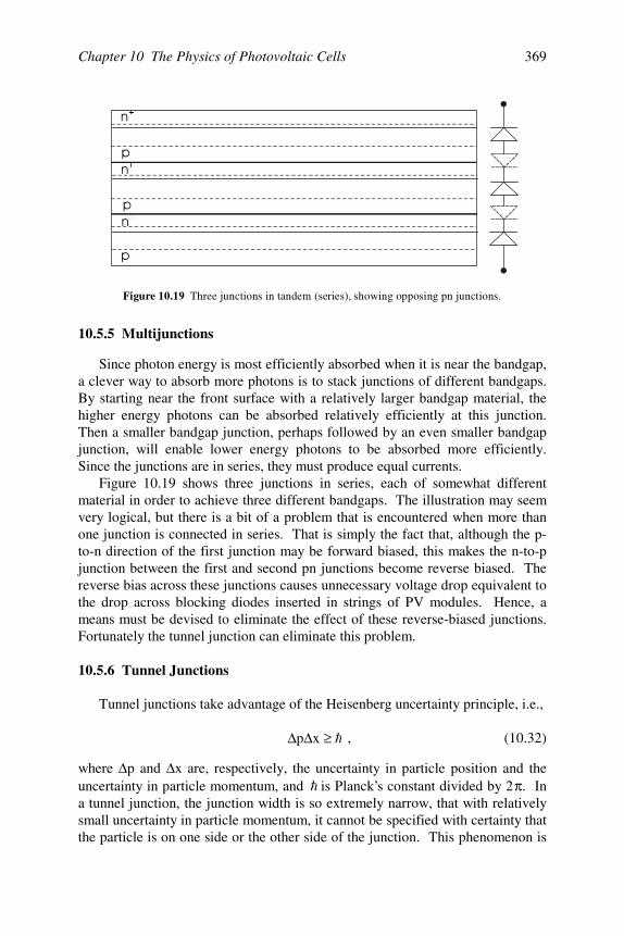
Chapter 10 The Physics of Photovoltaic Cells 369
10.5.5 Multijunctions
Since photon energy is most efficiently absorbed when it is near the bandgap,a clever way to absorb more photons is to stack junctions of different bandgaps.By starting near the front surface with a relatively larger bandgap material, thehigher energy photons can be absorbed relatively efficiently at this junction.Then a smaller bandgap junction, perhaps followed by an even smaller bandgapjunction, will enable lower energy photons to be absorbed more efficiently.Since the junctions are in series, they must produce equal currents.
Figure 10.19 shows three junctions in series, each of somewhat differentmaterial in order to achieve three different bandgaps. The illustration may seemvery logical, but there is a bit of a problem that is encountered when more thanone junction is connected in series. That is simply the fact that, although the p-to-n direction of the first junction may be forward biased, this makes the n-to-pjunction between the first and second pn junctions become reverse biased. Thereverse bias across these junctions causes unnecessary voltage drop equivalent tothe drop across blocking diodes inserted in strings of PV modules. Hence, ameans must be devised to eliminate the effect of these reverse-biased junctions.Fortunately the tunnel junction can eliminate this problem.
10.5.6 Tunnel Junctions
Tunnel junctions take advantage of the Heisenberg uncertainty principle, i.e.,
≥∆∆ xp , (10.32)
where ∆ p and ∆ x are, respectively, the uncertainty in particle position and theuncertainty in particle momentum, and is Planck’s constant divided by 2 π . Ina tunnel junction, the junction width is so extremely narrow, that with relativelysmall uncertainty in particle momentum, it cannot be specified with certainty thatthe particle is on one side or the other side of the junction. This phenomenon is
Figure 10.19 Three junctions in tandem (series), showing opposing pn junctions.
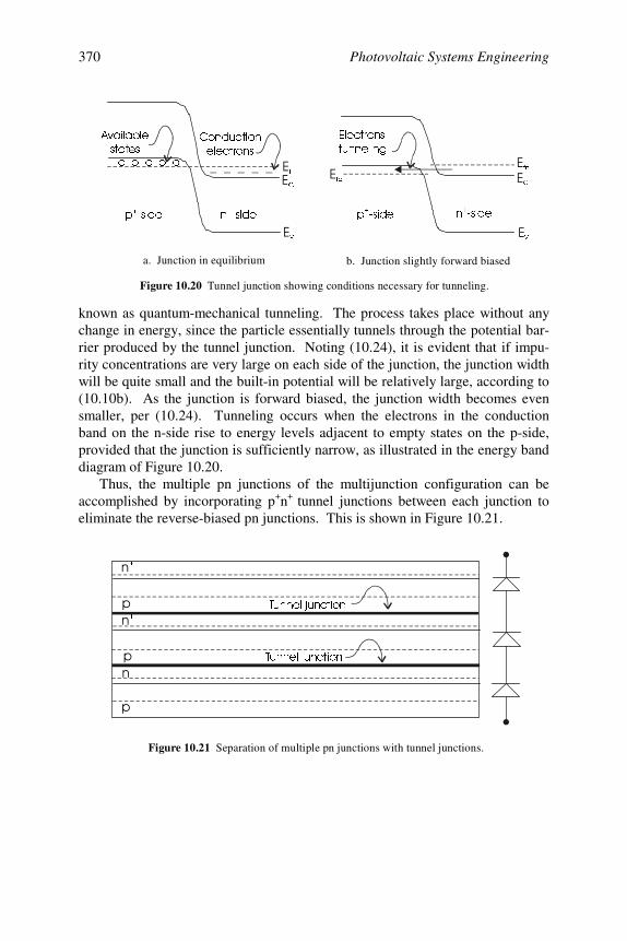
Photovoltaic Systems Engineering370
known as quantum-mechanical tunneling. The process takes place without anychange in energy, since the particle essentially tunnels through the potential bar-rier produced by the tunnel junction. Noting (10.24), it is evident that if impu-rity concentrations are very large on each side of the junction, the junction widthwill be quite small and the built-in potential will be relatively large, according to(10.10b). As the junction is forward biased, the junction width becomes evensmaller, per (10.24). Tunneling occurs when the electrons in the conductionband on the n-side rise to energy levels adjacent to empty states on the p-side,provided that the junction is sufficiently narrow, as illustrated in the energy banddiagram of Figure 10.20.
Thus, the multiple pn junctions of the multijunction configuration can beaccomplished by incorporating p+n+ tunnel junctions between each junction toeliminate the reverse-biased pn junctions. This is shown in Figure 10.21.
RRRRR
&RQGXFWLRQHOHFWURQV
$YDLODEOHVWDWHV
S VLGH S VLGH
Q VLGH Q VLGH
I IS
IQ
&&
9 9
(OHFWURQVWXQQHOLQJ
Figure 10.20 Tunnel junction showing conditions necessary for tunneling.
a. Junction in equilibrium b. Junction slightly forward biased
7XQQHOMXQFWLRQ
7XQQHOMXQFWLRQ
Figure 10.21 Separation of multiple pn junctions with tunnel junctions.
Chapter 10 The Physics of Photovoltaic Cells 371
Problems
10.1 What can be said about the bandgap of glass? Why is silicon opaque?For what range of wavelengths will silicon appear transparent?
10.2 Given the arguments about direct vs. indirect bandgap materials and theability of these materials to absorb photons, offer an argument about theoptimal bandgap structure of a material that will emit photons efficiently.Note that photon emission involves a transition of an electron from theconduction band to the valence band.
10.3 What would the bandgap need to be for an infrared LED? What about ared LED? What about a green LED? What about a blue LED? Wouldyou expect the materials with these bandgaps to be direct bandgap materi-als or indirect bandgap materials?
10.4 Compare the average thermal velocity of an electron, vth, at room tem-perature, if ½mvth
2 = ½kT, where m is the electron mass, k is Boltz-mann’s constant and T is the absolute temperature, with the drift velocityof an electron having a mobility of 103 cm2/volt-sec in an electric field of1000 V/cm. The drift velocity equals the product of the mobility and theelectric field. At what electric field strength will the drift velocity equalthe thermal velocity?
10.5 Use (10.9b) to solve for the concentration of electrons as a function ofposition between the neutral n-side edge of the junction and the edge ofthe neutral p-side of the junction. Plot this concentration function on alogarithmic scale along with the concentration of ionized impurities in thespace charge layer.
10.6 Solve for the concentration of holes in the space charge layer. Show thatin the space charge layer in thermal equilibrium, that np = ni
2 at every po-sition, x.
10.7 Show that (10.10b) can also be obtained by setting the net hole currentacross the junction equal to zero.
10.8 If a material has n = 8600 cm2/volt-sec, p = 400 cm2/volt-sec and n = p
= 10 ns, would you design a PV cell with the light incident on the n-sideor the p-side of the material? Approximately what should be the distancebetween the edge of the space charge layer and the back contact? Explainwhy.
10.9 Show that (10.24) results from adding (10.23a) to (10.23b).
Photovoltaic Systems Engineering372
10.10 Show that combining (10.10b) and (10.24) results in (10.25).
10.11 Assume NA = 1020 cm–3 and ND = 1017 cm–3 . Assume room tempera-ture.a. Calculate the built-in junction potential for Si and GaAs.b. Calculate the junction width for Si and for GaAs under short-circuit
conditions.
10.12 Use (10.30) to calculate the electric field in the n-region adjacent to thejunction if the donor concentration is given by ND(x) = NS(1 – bx), wherex is distance measured from the surface of the cell and b is a constant.
10.13 Calculate the widths of the following abrupt junctions in Si at room tem-perature with no external bias applied.a. NA = 1016 and ND = 1020.b. NA = 1021 and ND = 1021.Next, calculate the widths of each junction if a forward bias of 0.3 V isapplied, with all the external voltage appearing across the junction.Sketch the energy band picture for part b.
References
[1] Yang, E. S., Microelectronic Devices, McGraw-Hill, New York, 1988.[2] Streetman, B. G., Solid State Electronic Devices, 4th Ed., Prentice Hall, Englewood
Cliffs, NJ, 1995.[3] Hu, C. and White, R. M., Solar Cells: From Basic to Advanced Systems, McGraw-
Hill, New York, 1983.[4] Rappaport, P., RCA Review, Vol 20, September 1959, 373–379.[5] Zweibel, K., Harnessing Solar Power, Plenum Press, New York, 1990.
373
Chapter 11PRESENT AND PROPOSED PV CELLS
11.1 Introduction
In the last chapter, the basic theory of PV cells was presented without regardto any specific cell technology. This chapter will cover some of the fabricationprocesses associated with current cells along with discussions of the operation ofa variety of cells, some of which are commonly in use and others of which arestill in the experimental phases.
Progress in PV research and development is moving so rapidly that by thetime this chapter is in print, much of it will likely be outdated. Hence, in addi-tion to introducing the reader to technologies of the early 2000s, it is also thegoal of this chapter to provide the reader with the intellectual tools needed toread and understand current literature. Many of the sources of current informa-tion on PV technology are listed in the reference section of the chapter.
In general, cell fabrication begins with the refining and purification of thecell base material. After extremely pure material is available, then the pn junc-tion must be formed. In some multiple-layer cells, more than one junction isformed along with various fascinating isolation steps. The single crystal siliconcell has made its mark on history. Whether it will continue to make its mark onthe future will depend on reducing the amount of energy consumed in the pro-duction of the cell. Its fabrication and characteristics will be discussed first.During the discussion of the single crystal silicon cell, important processes, suchas crystal growth and diffusion will be discussed. These basic processes inmany cases are applicable to the fabrication of other types of PV cells. Impor-tant new developments in crystalline Si cell technology are centered around thethin Si cell, which will also be discussed.
Perhaps the most promising future PV cells will consist of thin films. Cer-tain materials have direct bandgaps with energies near the peak of the solarspectrum, along with relatively high absorption constants and the capability ofbeing fabricated with pn junctions. These films are not single crystal devices, sothere are limitations to carrier mobilities and subsequent device performance.However, in spite of the non-single-crystal structures, laboratory conversionefficiencies in excess of 20% have been achieved [1].
Thin films are advantageous because only a minimal amount of material is photon current vs. optical path length for common thin film materials. Note thatwithin 1 to 2 µm all the materials approach photon current saturation, whereascrystalline Si requires significantly greater thickness for full photon absorption.Examples of thin film PV cells that are currently under serious consideration areamorphous silicon (a-Si), copper indium (gallium) diselenide (CIGS) and cad-mium telluride (CdTe). At the time of this writing, a-Si and CIGS modules arein commercial production and CdTe modules are undergoing commercial scale
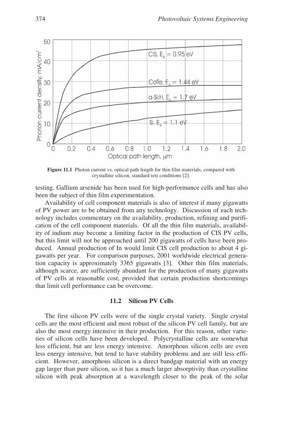
Photovoltaic Systems Engineering374
testing. Gallium arsenide has been used for high-performance cells and has alsobeen the subject of thin film experimentation.
Availability of cell component materials is also of interest if many gigawattsof PV power are to be obtained from any technology. Discussion of each tech-nology includes commentary on the availability, production, refining and purifi-cation of the cell component materials. Of all the thin film materials, availabil-ity of indium may become a limiting factor in the production of CIS PV cells,but this limit will not be approached until 200 gigawatts of cells have been pro-duced. Annual production of In would limit CIS cell production to about 4 gi-gawatts per year. For comparison purposes, 2001 worldwide electrical genera-tion capacity is approximately 3365 gigawatts [3]. Other thin film materials,although scarce, are sufficiently abundant for the production of many gigawattsof PV cells at reasonable cost, provided that certain production shortcomingsthat limit cell performance can be overcome.
11.2 Silicon PV Cells
The first silicon PV cells were of the single crystal variety. Single crystalcells are the most efficient and most robust of the silicon PV cell family, but arealso the most energy intensive in their production. For this reason, other varie-ties of silicon cells have been developed. Polycrystalline cells are somewhatless efficient, but are less energy intensive. Amorphous silicon cells are evenless energy intensive, but tend to have stability problems and are still less effi-cient. However, amorphous silicon is a direct bandgap material with an energygap larger than pure silicon, so it has a much larger absorptivity than crystallinesilicon with peak absorption at a wavelength closer to the peak of the solar
Figure 11.1 Photon current vs. optical path length for thin film materials, compared withcrystalline silicon, standard test conditions [2].
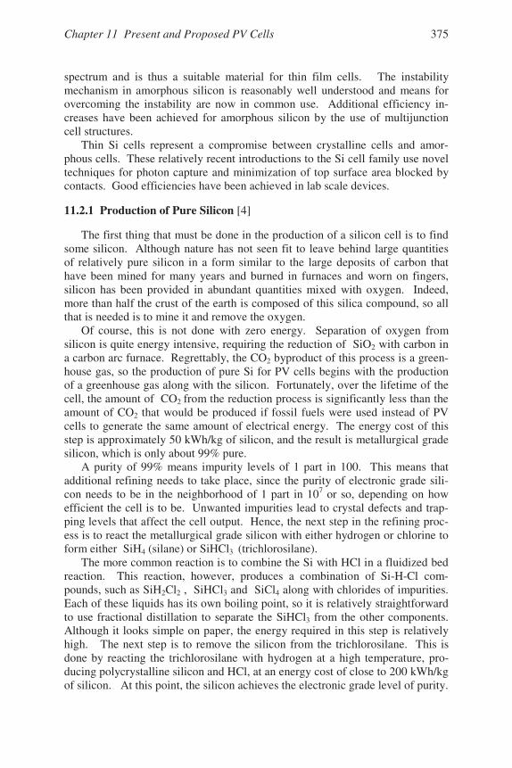
Chapter 11 Present and Proposed PV Cells 375
spectrum and is thus a suitable material for thin film cells. The instabilitymechanism in amorphous silicon is reasonably well understood and means forovercoming the instability are now in common use. Additional efficiency in-creases have been achieved for amorphous silicon by the use of multijunctioncell structures.
Thin Si cells represent a compromise between crystalline cells and amor-phous cells. These relatively recent introductions to the Si cell family use noveltechniques for photon capture and minimization of top surface area blocked bycontacts. Good efficiencies have been achieved in lab scale devices.
11.2.1 Production of Pure Silicon [4]
The first thing that must be done in the production of a silicon cell is to findsome silicon. Although nature has not seen fit to leave behind large quantitiesof relatively pure silicon in a form similar to the large deposits of carbon thathave been mined for many years and burned in furnaces and worn on fingers,silicon has been provided in abundant quantities mixed with oxygen. Indeed,more than half the crust of the earth is composed of this silica compound, so allthat is needed is to mine it and remove the oxygen.
Of course, this is not done with zero energy. Separation of oxygen fromsilicon is quite energy intensive, requiring the reduction of SiO2 with carbon ina carbon arc furnace. Regrettably, the CO2 byproduct of this process is a green-house gas, so the production of pure Si for PV cells begins with the productionof a greenhouse gas along with the silicon. Fortunately, over the lifetime of thecell, the amount of CO2 from the reduction process is significantly less than theamount of CO2 that would be produced if fossil fuels were used instead of PVcells to generate the same amount of electrical energy. The energy cost of thisstep is approximately 50 kWh/kg of silicon, and the result is metallurgical gradesilicon, which is only about 99% pure.
A purity of 99% means impurity levels of 1 part in 100. This means thatadditional refining needs to take place, since the purity of electronic grade sili-con needs to be in the neighborhood of 1 part in 107 or so, depending on howefficient the cell is to be. Unwanted impurities lead to crystal defects and trap-ping levels that affect the cell output. Hence, the next step in the refining proc-ess is to react the metallurgical grade silicon with either hydrogen or chlorine toform either SiH4 (silane) or SiHCl3 (trichlorosilane).
The more common reaction is to combine the Si with HCl in a fluidized bedreaction. This reaction, however, produces a combination of Si-H-Cl com-pounds, such as SiH2Cl2 , SiHCl3 and SiCl4 along with chlorides of impurities.Each of these liquids has its own boiling point, so it is relatively straightforwardto use fractional distillation to separate the SiHCl3 from the other components.Although it looks simple on paper, the energy required in this step is relativelyhigh. The next step is to remove the silicon from the trichlorosilane. This isdone by reacting the trichlorosilane with hydrogen at a high temperature, pro-ducing polycrystalline silicon and HCl, at an energy cost of close to 200 kWh/kgof silicon. At this point, the silicon achieves the electronic grade level of purity.
Photovoltaic Systems Engineering376
11.2.2 Single Crystal Silicon Cells
Fabrication of the WaferTo produce single crystal silicon from the polycrystalline material, the sili-
con must be melted and recrystallized. This is done by dipping a silicon seedcrystal into the melt and slowly withdrawing it from the melt with a slighttwisting motion. As the silicon is pulled from the melt, it reaches a somewhathigher purity level since the remaining impurities tend to remain behind in themelt. Under properly controlled conditions for solidification and replenishmentof the melt, crystals as large as 4 to 6 inches in diameter and 3 to 5 feet long canbe readily grown.
To produce n-type or p-type crystals, boron or arsenic can be introduced tothe melt in whatever quantities are needed to produce the desired doping levels.Other type III or type V materials may also be introduced, but generally the dif-fusion constants or activation energies of these materials are less desirable froma PV performance perspective. Indium, for example, is a group III impurity, butat room temperature, because of the higher activation energy of indium, a sig-
Figure 11.2 Production of single crystal silicon wafers from sand [5].(Adapted from Ciszek, T. F., 1988, IEEE.)C
Chapter 11 Present and Proposed PV Cells 377
nificant percentage of the indium atoms do not ionize and donate holes to thehost crystal. Phosphorous is a group V impurity that has satisfactory ionizationproperties, but also has a higher diffusion constant in silicon, so that if the hostmaterial is heated, phosphorous atoms will migrate in the host material at afaster rate than arsenic atoms.
Special saws are then used to cut the ingots into wafers. Since circular wa-fers mounted in a module leave a large amount of empty space between the wa-fers, often times the edges of the wafers are trimmed to make the wafers closerto square. The wafers are approximately 0.01 inch thick and are quite brittle.The sawing causes significant surface damage, so the wafers must next bechemically etched to restore the surface. In order to achieve the textured finishas described in the last chapter, it is possible to use a preferential etching proc-ess, so that after etching, the wafer surface is textured and relatively defect free.Again, the wafering process is quite energy intensive.
Fabrication of the Junction [6]The next step in the production of the single crystal silicon cell is to create
the pn junction. In electronic semiconductors, pn junctions can be created bydiffusion, epitaxial growth and ion implantation. These methods work fine forjunctions having areas in the 10−12 m2 range, but for PV cells with junction areasin the 10−2 m2 range, the time it takes to produce a given area of junction be-comes very important. Hence, due to cost constraints, pn junctions in crystallinesilicon PV cells are made primarily by diffusion.
Impurity atoms diffuse into silicon in a manner similar to the diffusion ofholes and electrons across regions of nonuniform impurity density. The con-centration as a function of distance from the surface, x, and time is determinedby the solution of the familiar diffusion equation
2
2
x
ND
t
N
∂∂=
∂∂ , (11.1)
where N represents the density of the impurity and D is the diffusion constantassociated with the specific impurity. It should be noted that D is highly tem-perature dependent, especially close to the melting temperature of the host mate-rial. At room temperature, diffusion is negligible, but in the neighborhood of1000oC, diffusion becomes appreciable.
The solution to (11.1) depends upon the boundary conditions imposed on theimpurity. Most diffusion processes begin by holding the surface concentrationof impurities constant for a fixed time. Then the impurity source is removed sothe total number of impurities now remains constant, equal to the number ofimpurity atoms that diffused into the host during the constant surface concentra-tion step of the process. The first step, known as the predeposition, leads to thewell-known complimentary error function solution, i.e.,
Dt2
xerfcN)t,x(N o= , (11.2)
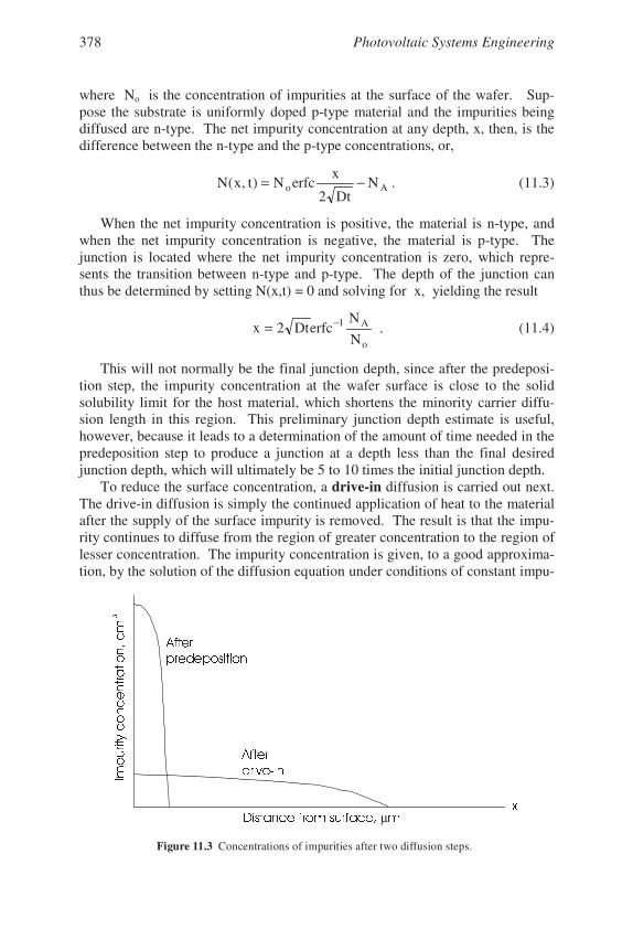
Photovoltaic Systems Engineering378
where No is the concentration of impurities at the surface of the wafer. Sup-pose the substrate is uniformly doped p-type material and the impurities beingdiffused are n-type. The net impurity concentration at any depth, x, then, is thedifference between the n-type and the p-type concentrations, or,
Ao NDt2
xerfcN)t,x(N −= . (11.3)
When the net impurity concentration is positive, the material is n-type, andwhen the net impurity concentration is negative, the material is p-type. Thejunction is located where the net impurity concentration is zero, which repre-sents the transition between n-type and p-type. The depth of the junction canthus be determined by setting N(x,t) = 0 and solving for x, yielding the result
o
A1
N
NerfcDt2x −= . (11.4)
This will not normally be the final junction depth, since after the predeposi-tion step, the impurity concentration at the wafer surface is close to the solidsolubility limit for the host material, which shortens the minority carrier diffu-sion length in this region. This preliminary junction depth estimate is useful,however, because it leads to a determination of the amount of time needed in thepredeposition step to produce a junction at a depth less than the final desiredjunction depth, which will ultimately be 5 to 10 times the initial junction depth.
To reduce the surface concentration, a drive-in diffusion is carried out next.The drive-in diffusion is simply the continued application of heat to the materialafter the supply of the surface impurity is removed. The result is that the impu-rity continues to diffuse from the region of greater concentration to the region oflesser concentration. The impurity concentration is given, to a good approxima-tion, by the solution of the diffusion equation under conditions of constant impu-
µ
Figure 11.3 Concentrations of impurities after two diffusion steps.
Chapter 11 Present and Proposed PV Cells 379
rities per unit area. The assumption is that all of the impurities diffused into thematerial during the predeposition step remain at the surface of the material. Thenumber of impurities per unit area can be determined by integrating (11.3) fromthe surface into the material. While the actual distance of travel of the impuri-
π== ∫
∞Dt
N2dx)t,x(N)t(Q o
0
. (11.5)
After the drive-in step, the net impurity concentration is represented fairly accu-rately by the Gaussian distribution function,
ADt4
x
NeDt
Q)t,x(N
2
−π
=−
. (11.6)
This expression can now be solved for the junction depth by again settingN(x,t) = 0. The solution is left as an exercise for the reader (Problem 11.2). It isthus a straightforward matter to control the diffusion of impurities into the waferto produce a junction at any desired depth from the surface. Since it is desirableto have the junction within a minority carrier diffusion length of the surface, thedepth can be set to achieve this goal. Note that (11.3) through (11.6) also enablethe cell designer to control the impurity concentration profile on the n-side ofthe junction. Figure 11.3 shows the impurity concentrations after the two diffu-sion steps have been completed.
ContactsAfter creating the pn junction, the next step is to affix contacts to the cell. If
the intent is to fabricate contacts that will last as long as the rest of the cell, thenalligator clips are somewhat inadequate. It is necessary to affix contacts that arelow resistance ohmic contacts that will remain in good contact with the cellthrough extreme temperature cycling. The contact material must lend itself tobonding of connecting wires so the cell can be integrated into a module.
The back contact covers the entire cell and is commonly made of evaporatedaluminum that is annealed by heating the material after evaporation. The an-nealing process causes the aluminum to diffuse slightly into the silicon, creatinga strong bond that will not break under thermal cycling. Since aluminum is agroup III element, it also acts as a p-type donor and produces a heavily doped p-region adjoining the contact. This heavily doped p-region creates an impuritygradient that produces a resulting electric field that accelerates holes toward theback contact.
The front contact is considerably more challenging for several reasons. Firstof all, if the front contact is opaque to light, then it will block photons from en-tering the cell and being absorbed. This means the area of the front contact mustbe minimized. On the other hand, if the area is too small, then the resistance ofthe contact increases. Since the junction is only a small distance below the front
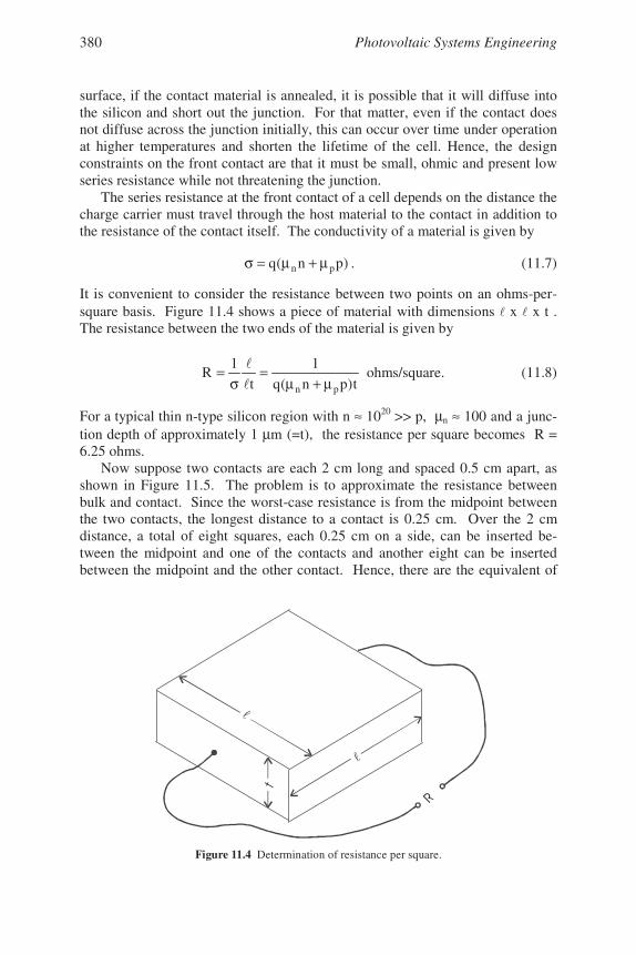
Photovoltaic Systems Engineering380
surface, if the contact material is annealed, it is possible that it will diffuse intothe silicon and short out the junction. For that matter, even if the contact doesnot diffuse across the junction initially, this can occur over time under operationat higher temperatures and shorten the lifetime of the cell. Hence, the designconstraints on the front contact are that it must be small, ohmic and present lowseries resistance while not threatening the junction.
The series resistance at the front contact of a cell depends on the distance thecharge carrier must travel through the host material to the contact in addition tothe resistance of the contact itself. The conductivity of a material is given by
)pn(q pn µ+µ=σ . (11.7)
It is convenient to consider the resistance between two points on an ohms-per-square basis. Figure 11.4 shows a piece of material with dimensions x x t .The resistance between the two ends of the material is given by
t)pn(q
1
t
1R
pn µ+µ=
σ=
ohms/square. (11.8)
For a typical thin n-type silicon region with n ≈ 1020 >> p, µn ≈ 100 and a junc-tion depth of approximately 1 µm (=t), the resistance per square becomes R =6.25 ohms.
Now suppose two contacts are each 2 cm long and spaced 0.5 cm apart, asshown in Figure 11.5. The problem is to approximate the resistance betweenbulk and contact. Since the worst-case resistance is from the midpoint betweenthe two contacts, the longest distance to a contact is 0.25 cm. Over the 2 cmdistance, a total of eight squares, each 0.25 cm on a side, can be inserted be-tween the midpoint and one of the contacts and another eight can be insertedbetween the midpoint and the other contact. Hence, there are the equivalent of
Figure 11.4 Determination of resistance per square.
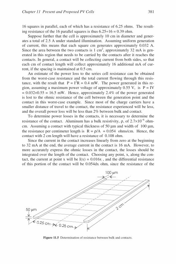
Chapter 11 Present and Proposed PV Cells 381
16 squares in parallel, each of which has a resistance of 6.25 ohms. The result-ing resistance of the 16 parallel squares is thus 6.25÷16 = 0.39 ohm.
Suppose further that the cell is approximately 10 cm in diameter and gener-ates a total of 2.5 A under standard illumination. Assuming uniform generationof current, this means that each square cm generates approximately 0.032 A.Since the area between the two contacts is 1 cm2, approximately 32 mA is gen-erated in this region that needs to be carried by the contacts after it reaches thecontacts. In general, a contact will be collecting current from both sides, so thateach cm of contact length will collect approximately 16 additional mA of cur-rent, if the spacing is maintained at 0.5 cm.
An estimate of the power loss to the series cell resistance can be obtainedfrom the worst-case resistance and the total current flowing through this resis-tance, with the result that P = I2R = 0.4 mW. The power generated in this re-gion, assuming a maximum power voltage of approximately 0.55 V, is P = IV= 0.032×0.55 = 16.5 mW. Hence, approximately 2.4% of the power generatedis lost to the ohmic resistance of the cell between the generation point and thecontact in this worst-case example. Since most of the charge carriers have asmaller distance of travel to the contact, the resistance experienced will be less,and the overall power loss will be less than 2% between bulk and contact.
To determine power losses in the contacts, it is necessary to determine theresistance of the contact. Aluminum has a bulk resistivity, ρ, of 2.7×10⁻⁶ ohm-cm. Assuming a contact with typical thickness of 50 µm and width of 100 µm,the resistance per centimeter length is R = ρ/A = 0.054 ohms/cm. Hence, thecontact with 2 cm length will have a resistance of 0.108 ohm.
Since the current in the contact increases linearly from zero at the beginningto 32 mA at the end, the average current in the contact is 16 mA. However, tomore accurately express the ohmic losses in the contact, the losses should beintegrated over the length of the contact. Choosing any point, x, along the con-tact, the current at point x will be I(x) = 0.016x , and the differential resistanceof this portion of the contact will be 0.054dx ohm, since the resistance of the
µ
µ
Figure 11.5 Determination of resistance between bulk and contacts.
Photovoltaic Systems Engineering382
contact is 0.054 ohm/cm of length. The result of this calculation is
∫ ∫ −×===2
0
52
0
22 107.3dx054.)x016(.)RI(dP watts. (11.9)
This is only about 10% of the power loss over the cell surface. Hence, mostof the series resistance is due to the surface resistivity of the bulk cell material.However, if the contact is only 5 µm thick, the resistance increases by a factor of10 and the power loss is comparable to the bulk losses. These calculations il-lustrate a means that may be used to determine optimal spacing between topcontacts as well as the dimensions of the top contacts to keep power losses to aminimum while still enabling maximum photon absorption.
As the current in the contacts continues to increase, the cross-sectional areaof the contact must increase to enable the contact to carry the total current withinacceptable voltage drop limitations. This is analogous to the circulatory systemof plants, in which leaves contain capillaries that extend over the leaf to providetransport for nutrients.
The front contacts can be fabricated by several means, including evaporationin a vacuum chamber or silk screening with a paste. For fine lines, the lines maybe defined with photoresist as is done in the production of small geometry elec-tronic semiconductors.
If aluminum is the contact material, in order to make an ohmic contact to then-type material, it is necessary to anneal the contact for approximately 5 minutesat a temperature of approximately 450°C. To prevent transport of the aluminumthrough to the junction, it is advisable to use a small percentage of silicon in thealuminum or to first evaporate a very thin (≈ 0.01 µm) layer of titanium orchromium to act as a barrier to the aluminum diffusing into the junction.
Antireflective CoatingAfter affixing the contacts to the material, an antireflective coating may be
applied to the cell, normally by evaporation, since the coating must be so thin.A quarter wavelength coating has a thickness of approximately 0.15 µm. Thesecoatings are commonly used for photographic lenses to increase their speed byreducing reflection and simultaneously increasing transmission. Typical coat-ings are listed in Table 10.2. As long as the photon wavelength is relativelyclose to the quarter-wavelength constraint, transmission in excess of 90% canbe achieved for the cell surface.
Because antireflective coatings optimize transmission at only one wave-length, textured cell surfaces are becoming more common for enhancing lighttrapping over the full spectrum.
ModulesThe cells must then be mounted in modules, with interconnecting wires or
metal foil strips. The interconnects are typically ultrasonically bonded to thecell contacts. The cells are then mounted to the module base and encapsulated
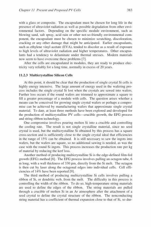
Chapter 11 Present and Proposed PV Cells 383
with a glass or composite. The encapsulant must be chosen for long life in thepresence of ultraviolet radiation as well as possible degradation from other envi-ronmental factors. Depending on the specific module environment, such asblowing sand, salt spray, acid rain or other not-so-friendly environmental com-ponent, the encapsulant must be chosen to minimize scratching, discoloration,cracking or any other damage that might be anticipated. Earlier encapsulants,such as ethylene vinyl acetate (EVA), tended to discolor as a result of exposureto high levels of ultraviolet radiation and higher temperatures. Other encapsu-lants had a tendency to delaminate under thermal stresses. Modern materialsnow seem to have overcome these problems [7].
After the cells are encapsulated in modules, they are ready to produce elec-tricity very reliably for a long time, normally in excess of 20 years.
11.2.3 Multicrystalline Silicon Cells
At this point, it should be clear that the production of single crystal Si cells ishighly energy intensive. The large amount of energy used in the wafering pro-cess includes the single crystal Si lost when the crystals are sawed into wafers.Further loss occurs if the round wafers are trimmed to approximate a square tofill a greater percentage of a module with cells. The question arises whether ameans can be conceived for growing single crystal wafers or perhaps a compro-mise can be achieved by manufacturing wafers that approximate single crystalmaterial. To date, at least three methods have been explored and developed forthe production of multicrystalline PV cells—crucible growth, the EFG processand string ribbon technology.
One compromise involves pouring molten Si into a crucible and controllingthe cooling rate. The result is not single crystalline material, since no seedcrystal is used, but the multicrystalline Si obtained by this process has a squarecross-section and is sufficiently close to the single crystal ideal that efficienciesin the range of 15% can be obtained. It is still necessary to saw the ingots intowafers, but the wafers are square, so no additional sawing is needed, as was thecase with the round Si ingots. This process increases the production rate per kgof material by reducing the kerf loss.
Another method of producing multicrystalline Si is the edge-defined film-fedgrowth (EFG) method [8]. The EFG process involves pulling an octagon tube, 6m long, with a wall thickness of 330 µm, directly from the Si melt. The octagonis then cut by laser along the octagonal edges into individual cells. Cell effi-ciencies of 14% have been reported [9].
The third method of producing multicrystalline Si cells involves pulling aribbon of Si, or dendritic web, from the melt. The difficulty in this process iscontrolling the width of the ribbon. To do so, high-temperature string materialsare used to define the edges of the ribbon. The string materials are pulledthrough a crucible of molten Si in an Ar atmosphere after the attachment of aseed crystal to define the crystal structure of the ribbon. The nonconductingstring material has a coefficient of thermal expansion close to that of Si, so dur-
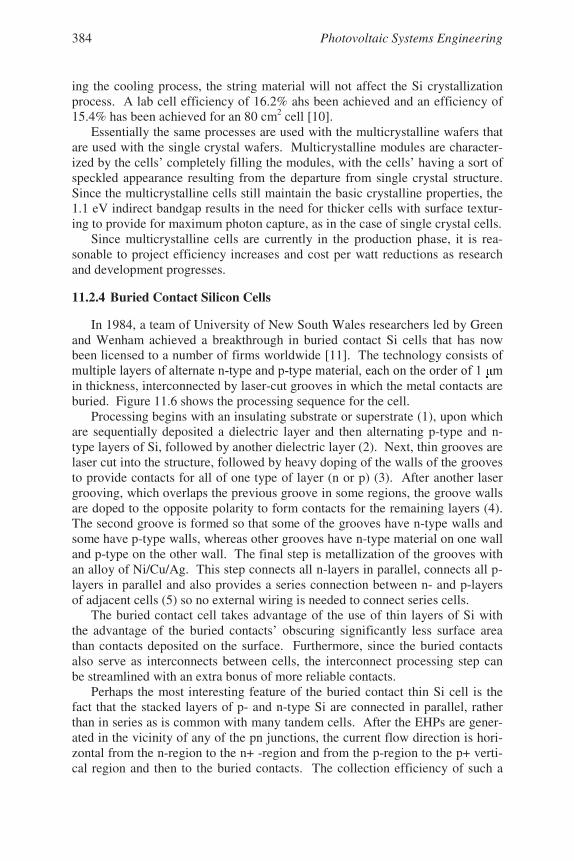
Photovoltaic Systems Engineering384
ing the cooling process, the string material will not affect the Si crystallizationprocess. A lab cell efficiency of 16.2% ahs been achieved and an efficiency of15.4% has been achieved for an 80 cm2 cell [10].
Essentially the same processes are used with the multicrystalline wafers thatare used with the single crystal wafers. Multicrystalline modules are character-ized by the cells’ completely filling the modules, with the cells’ having a sort ofspeckled appearance resulting from the departure from single crystal structure.Since the multicrystalline cells still maintain the basic crystalline properties, the1.1 eV indirect bandgap results in the need for thicker cells with surface textur-ing to provide for maximum photon capture, as in the case of single crystal cells.
Since multicrystalline cells are currently in the production phase, it is rea-sonable to project efficiency increases and cost per watt reductions as researchand development progresses.
11.2.4 Buried Contact Silicon Cells
In 1984, a team of University of New South Wales researchers led by Greenand Wenham achieved a breakthrough in buried contact Si cells that has nowbeen licensed to a number of firms worldwide [11]. The technology consists of in thickness, interconnected by laser-cut grooves in which the metal contacts areburied. Figure 11.6 shows the processing sequence for the cell.
Processing begins with an insulating substrate or superstrate (1), upon whichare sequentially deposited a dielectric layer and then alternating p-type and n-type layers of Si, followed by another dielectric layer (2). Next, thin grooves arelaser cut into the structure, followed by heavy doping of the walls of the groovesto provide contacts for all of one type of layer (n or p) (3). After another lasergrooving, which overlaps the previous groove in some regions, the groove wallsare doped to the opposite polarity to form contacts for the remaining layers (4).The second groove is formed so that some of the grooves have n-type walls andsome have p-type walls, whereas other grooves have n-type material on one walland p-type on the other wall. The final step is metallization of the grooves withan alloy of Ni/Cu/Ag. This step connects all n-layers in parallel, connects all p-layers in parallel and also provides a series connection between n- and p-layersof adjacent cells (5) so no external wiring is needed to connect series cells.
The buried contact cell takes advantage of the use of thin layers of Si withthe advantage of the buried contacts’ obscuring significantly less surface areathan contacts deposited on the surface. Furthermore, since the buried contactsalso serve as interconnects between cells, the interconnect processing step canbe streamlined with an extra bonus of more reliable contacts.
Perhaps the most interesting feature of the buried contact thin Si cell is thefact that the stacked layers of p- and n-type Si are connected in parallel, ratherthan in series as is common with many tandem cells. After the EHPs are gener-ated in the vicinity of any of the pn junctions, the current flow direction is hori-zontal from the n-region to the n+ -region and from the p-region to the p+ verti-cal region and then to the buried contacts. The collection efficiency of such a
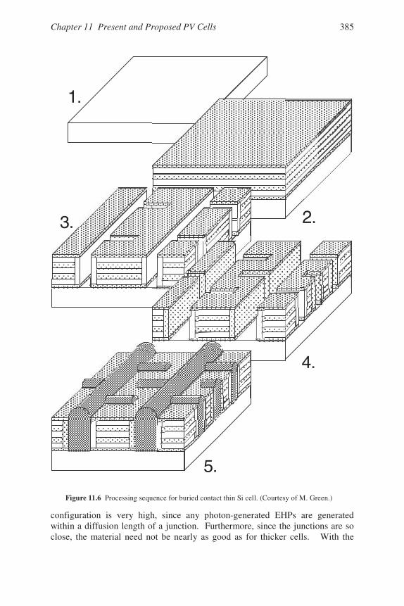
Chapter 11 Present and Proposed PV Cells 385
configuration is very high, since any photon-generated EHPs are generatedwithin a diffusion length of a junction. Furthermore, since the junctions are soclose, the material need not be nearly as good as for thicker cells. With the
Figure 11.6 Processing sequence for buried contact thin Si cell. (Courtesy of M. Green.)
1.
2.3.
4.
5.

Photovoltaic Systems Engineering386
elimination of the ingot and wafer processing steps, processing costs are reducedsignificantly. With the parallel conduction paths to the contacts, charge carrierstend to migrate to the paths of least resistance, leading to high fill factors.
An efficiency of 24.7% has been reported for a device with this cell structureand a flat plate module with an efficiency of 22.7% has been reported [12].
11.2.5. Other Thin Silicon Cells
A series of papers describing advances in this crystalline Si cells were pre-sented at the IEEE 29th Photovoltaic Specialists Conference in 2002. Thincrystalline cell technology has been pursued with the hope that cell efficiencycan be improved through the use of crystalline Si and that cell manufacturingcost can be lowered by using less material in the construction of the cell. Anumber of processes, including thin Si on ceramics [13], thin film crystallinesilicon on glass (CSG) [14], and epitaxial growth of Si on existing crystalline Siwith subsequent removal of the epitaxially grown cell from the existing Si sub-strate (the PSI Process) [15] are described in the Conference Proceedings.
The CSG process has produced modules of areas in the range of 480−900cm2 since 1998. Efficiencies have risen from 2% in 1999 to 8% in 2002. Thestructure consists of textured glass, antireflective coating, n+pp+ structure, resininsulator and metallization that dips into the structure from the back surface toform back and front cell contacts. The front contact does not require a transpar-ent conducting oxide (TCO), so losses from the TCO are eliminated. TCOs willbe discussed in more detail later in this chapter.
The modules consist of cells that are monolithically connected, and due toisolated metal interconnects that produce a fault-tolerant structure, performanceof the module is not degraded as the size is scaled up. The production cost ofthis module in May of 2002 was $1.95/W. Projections suggest a possible re-duction of cost to $1/W as the production process is improved.
Progress in the area of thin silicon cells over a relatively short period since1997 suggests that the reader may expect to see continued developments andimprovements of cells of this type.
11.2.6 Amorphous Silicon Cells
Amorphous silicon has no predictable crystal structure. Its atoms are locatedat more or less random angles and distances from each other. As a result, manyof the potential covalent bonds in the silicon are not completed. These incom-plete bonds cause a large number of equivalent impurity states in the bandgapand the noncrystalline nature of the material results in very low values for elec-tron and hole mobilities. The impurity states would typically result in trappingof mobile carriers, so the combination of impurity states and diminished trans-port properties at first rendered amorphous silicon as a rather poor semiconduc-tor material.
But persistent solid-state physicists confirmed that the incomplete bondscould be passivated with hydrogen, thus significantly reducing the number of
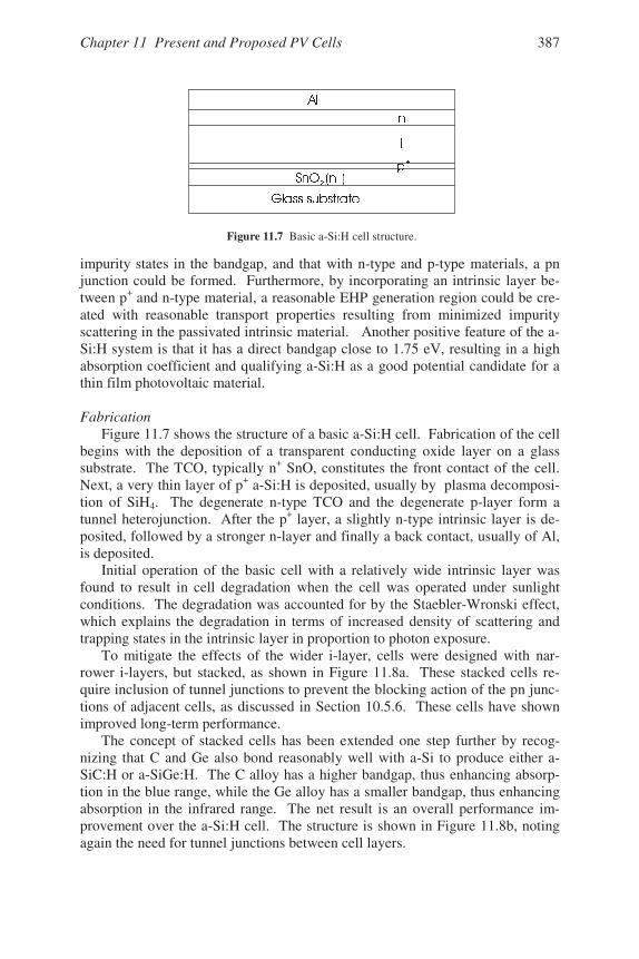
Chapter 11 Present and Proposed PV Cells 387
impurity states in the bandgap, and that with n-type and p-type materials, a pnjunction could be formed. Furthermore, by incorporating an intrinsic layer be-tween p+ and n-type material, a reasonable EHP generation region could be cre-ated with reasonable transport properties resulting from minimized impurityscattering in the passivated intrinsic material. Another positive feature of the a-Si:H system is that it has a direct bandgap close to 1.75 eV, resulting in a highabsorption coefficient and qualifying a-Si:H as a good potential candidate for athin film photovoltaic material.
FabricationFigure 11.7 shows the structure of a basic a-Si:H cell. Fabrication of the cell
begins with the deposition of a transparent conducting oxide layer on a glasssubstrate. The TCO, typically n+ SnO, constitutes the front contact of the cell.Next, a very thin layer of p+ a-Si:H is deposited, usually by plasma decomposi-tion of SiH4. The degenerate n-type TCO and the degenerate p-layer form atunnel heterojunction. After the p+ layer, a slightly n-type intrinsic layer is de-posited, followed by a stronger n-layer and finally a back contact, usually of Al,is deposited.
Initial operation of the basic cell with a relatively wide intrinsic layer wasfound to result in cell degradation when the cell was operated under sunlightconditions. The degradation was accounted for by the Staebler-Wronski effect,which explains the degradation in terms of increased density of scattering andtrapping states in the intrinsic layer in proportion to photon exposure.
To mitigate the effects of the wider i-layer, cells were designed with nar-rower i-layers, but stacked, as shown in Figure 11.8a. These stacked cells re-quire inclusion of tunnel junctions to prevent the blocking action of the pn junc-tions of adjacent cells, as discussed in Section 10.5.6. These cells have shownimproved long-term performance.
The concept of stacked cells has been extended one step further by recog-nizing that C and Ge also bond reasonably well with a-Si to produce either a-SiC:H or a-SiGe:H. The C alloy has a higher bandgap, thus enhancing absorp-tion in the blue range, while the Ge alloy has a smaller bandgap, thus enhancingabsorption in the infrared range. The net result is an overall performance im-provement over the a-Si:H cell. The structure is shown in Figure 11.8b, notingagain the need for tunnel junctions between cell layers.
Figure 11.7 Basic a-Si:H cell structure.
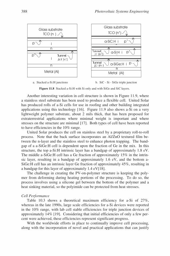
Photovoltaic Systems Engineering388
Another interesting variation in cell structure is shown in Figure 11.9, wherea stainless steel substrate has been used to produce a flexible cell. United Solarhas produced rolls of a-Si cells for use in roofing and other building integratedapplications using this technology [16]. Figure 11.9 also shows a-Si on a verylightweight polymer substrate, about 2 mils thick, that has been proposed forextraterrestrial applications where minimal weight is important and wherestresses on the structure are minimal [17]. Both types of cell have been reportedto have efficiencies in the 10% range.
United Solar produces the cell on stainless steel by a proprietary roll-to-rollprocess. Note that the back surface incorporates an Al/ZnO textured film be-tween the n-layer and the stainless steel to enhance photon trapping. The band-gap of a a-SiGe:H cell is dependent upon the fraction of Ge in the mix. In thisstructure, the top a-Si:H intrinsic layer has a bandgap of approximately 1.8 eV.The middle a-SiGe:H cell has a Ge fraction of approximately 15% in the intrin-sic layer, resulting in a bandgap of approximately 1.6 eV, and the bottom a-SiGe:H cell has an intrinsic layer Ge fraction of approximately 45%, resulting ina bandgap for this layer of approximately 1.4 eV[18].
The challenge in creating the PV-on-polymer structure is keeping the poly-mer from deforming during heating portions of the processing. To do so, theprocess involves using a silicone gel between the bottom of the polymer and aheat sinking material, so the polyimide can be protected from heat stresses.
Cell PerformanceTable 10.3 shows a theoretical maximum efficiency for a-Si of 27%,
whereas in the late 1990s, large scale efficiencies for a-Si devices were reportedin the 10% range, with lab cell stable efficiencies for triple junction devices ofapproximately 14% [19]. Considering that initial efficiencies of only a few per-cent were achieved, these efficiencies represent significant progress.
With the worldwide efforts in place to continually improve cell processing,along with the incorporation of novel and practical applications that can justify
a. Stacked a-Si:H junctions b. SiC - Si - SiGe triple junction
Figure 11.8 Stacked a-Si:H with Si only and with SiGe and SiC layers.
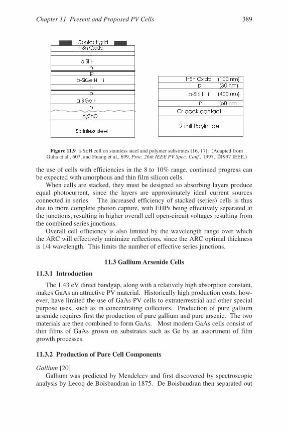
Chapter 11 Present and Proposed PV Cells 389
the use of cells with efficiencies in the 8 to 10% range, continued progress canbe expected with amorphous and thin film silicon cells.
When cells are stacked, they must be designed so absorbing layers produceequal photocurrent, since the layers are approximately ideal current sourcesconnected in series. The increased efficiency of stacked (series) cells is thusdue to more complete photon capture, with EHPs being effectively separated atthe junctions, resulting in higher overall cell open-circuit voltages resulting fromthe combined series junctions.
Overall cell efficiency is also limited by the wavelength range over whichthe ARC will effectively minimize reflections, since the ARC optimal thicknessis 1/4 wavelength. This limits the number of effective series junctions.
11.3 Gallium Arsenide Cells
11.3.1 Introduction
The 1.43 eV direct bandgap, along with a relatively high absorption constant,makes GaAs an attractive PV material. Historically high production costs, how-ever, have limited the use of GaAs PV cells to extraterrestrial and other specialpurpose uses, such as in concentrating collectors. Production of pure galliumarsenide requires first the production of pure gallium and pure arsenic. The twomaterials are then combined to form GaAs. Most modern GaAs cells consist ofthin films of GaAs grown on substrates such as Ge by an assortment of filmgrowth processes.
11.3.2 Production of Pure Cell Components
Gallium [20]Gallium was predicted by Mendeleev and first discovered by spectroscopic
analysis by Lecoq de Boisbaudran in 1875. De Boisbaudran then separated out
!
Figure 11.9 a-Si:H cell on stainless steel and polymer substrates [16, 17]. (Adapted from Guha et al., 607, and Huang et al., 699, 1997, 1997 IEEE.)Proc. 26th IEEE PV Spec. Conf., C
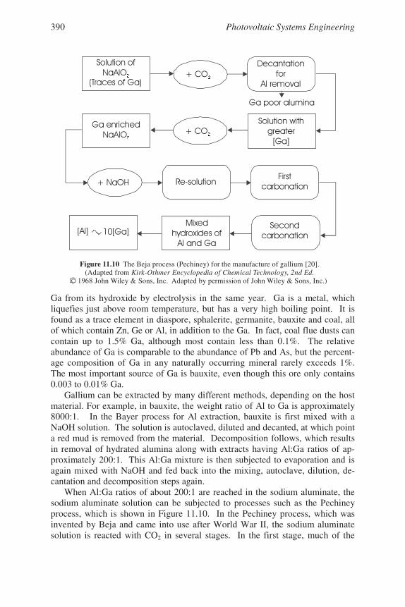
Photovoltaic Systems Engineering390
Ga from its hydroxide by electrolysis in the same year. Ga is a metal, whichliquefies just above room temperature, but has a very high boiling point. It isfound as a trace element in diaspore, sphalerite, germanite, bauxite and coal, allof which contain Zn, Ge or Al, in addition to the Ga. In fact, coal flue dusts cancontain up to 1.5% Ga, although most contain less than 0.1%. The relativeabundance of Ga is comparable to the abundance of Pb and As, but the percent-age composition of Ga in any naturally occurring mineral rarely exceeds 1%.The most important source of Ga is bauxite, even though this ore only contains0.003 to 0.01% Ga.
Gallium can be extracted by many different methods, depending on the hostmaterial. For example, in bauxite, the weight ratio of Al to Ga is approximately8000:1. In the Bayer process for Al extraction, bauxite is first mixed with aNaOH solution. The solution is autoclaved, diluted and decanted, at which pointa red mud is removed from the material. Decomposition follows, which resultsin removal of hydrated alumina along with extracts having Al:Ga ratios of ap-proximately 200:1. This Al:Ga mixture is then subjected to evaporation and isagain mixed with NaOH and fed back into the mixing, autoclave, dilution, de-cantation and decomposition steps again.
When Al:Ga ratios of about 200:1 are reached in the sodium aluminate, thesodium aluminate solution can be subjected to processes such as the Pechineyprocess, which is shown in Figure 11.10. In the Pechiney process, which wasinvented by Beja and came into use after World War II, the sodium aluminatesolution is reacted with CO2 in several stages. In the first stage, much of the
!"
#
$ !
%
!
#
&'()*
'+"
#" ,
+
-+'.+ -+ !+
)* )*
Figure 11.10 The Beja process (Pechiney) for the manufacture of gallium [20].(Adapted from
1968 John Wiley & Sons, Inc. Adapted by permission of John Wiley & Sons, Inc.)Kirk-Othmer Encyclopedia of Chemical Technology, 2nd Ed.
C
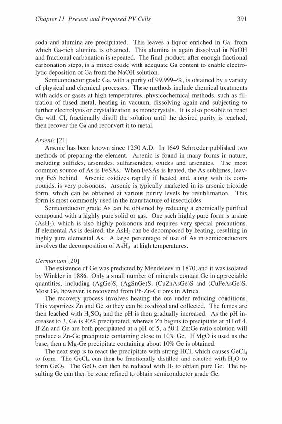
Chapter 11 Present and Proposed PV Cells 391
soda and alumina are precipitated. This leaves a liquor enriched in Ga, fromwhich Ga-rich alumina is obtained. This alumina is again dissolved in NaOHand fractional carbonation is repeated. The final product, after enough fractionalcarbonation steps, is a mixed oxide with adequate Ga content to enable electro-lytic deposition of Ga from the NaOH solution.
Semiconductor grade Ga, with a purity of 99.999+%, is obtained by a varietyof physical and chemical processes. These methods include chemical treatmentswith acids or gases at high temperatures, physicochemical methods, such as fil-tration of fused metal, heating in vacuum, dissolving again and subjecting tofurther electrolysis or crystallization as monocrystals. It is also possible to reactGa with Cl, fractionally distill the solution until the desired purity is reached,then recover the Ga and reconvert it to metal.
Arsenic [21]Arsenic has been known since 1250 A.D. In 1649 Schroeder published two
methods of preparing the element. Arsenic is found in many forms in nature,including sulfides, arsenides, sulfarsenides, oxides and arsenates. The mostcommon source of As is FeSAs. When FeSAs is heated, the As sublimes, leav-ing FeS behind. Arsenic oxidizes rapidly if heated and, along with its com-pounds, is very poisonous. Arsenic is typically marketed in its arsenic trioxideform, which can be obtained at various purity levels by resublimation. Thisform is most commonly used in the manufacture of insecticides.
Semiconductor grade As can be obtained by reducing a chemically purifiedcompound with a highly pure solid or gas. One such highly pure form is arsine(AsH3), which is also highly poisonous and requires very special precautions.If elemental As is desired, the AsH3 can be decomposed by heating, resulting inhighly pure elemental As. A large percentage of use of As in semiconductorsinvolves the decomposition of AsH3 at high temperatures.
Germanium [20]The existence of Ge was predicted by Mendeleev in 1870, and it was isolated
by Winkler in 1886. Only a small number of minerals contain Ge in appreciablequantities, including (AgGe)S, (AgSnGe)S, (CuZnAsGe)S and (CuFeAsGe)S.Most Ge, however, is recovered from Pb-Zn-Cu ores in Africa.
The recovery process involves heating the ore under reducing conditions.This vaporizes Zn and Ge so they can be oxidized and collected. The fumes arethen leached with H2SO4 and the pH is then gradually increased. As the pH in-creases to 3, Ge is 90% precipitated, whereas Zn begins to precipitate at pH of 4.If Zn and Ge are both precipitated at a pH of 5, a 50:1 Zn:Ge ratio solution willproduce a Zn-Ge precipitate containing close to 10% Ge. If MgO is used as thebase, then a Mg-Ge precipitate containing about 10% Ge is obtained.
The next step is to react the precipitate with strong HCl, which causes GeCl4
to form. The GeCl4 can then be fractionally distilled and reacted with H2O toform GeO2. The GeO2 can then be reduced with H2 to obtain pure Ge. The re-sulting Ge can then be zone refined to obtain semiconductor grade Ge.
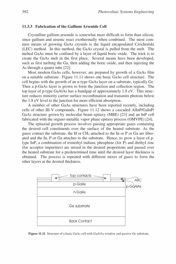
Photovoltaic Systems Engineering392
11.3.3 Fabrication of the Gallium Arsenide Cell
Crystalline gallium arsenide is somewhat more difficult to form than silicon,since gallium and arsenic react exothermally when combined. The most com-mon means of growing GaAs crystals is the liquid encapsulated Czochralski(LEC) method. In this method, the GaAs crystal is pulled from the melt. Themelted GaAs must be confined by a layer of liquid boric oxide. The trick is tocreate the GaAs melt in the first place. Several means have been developed,such as first melting the Ga, then adding the boric oxide, and then injecting theAs through a quartz tube [22].
Most modern GaAs cells, however, are prepared by growth of a GaAs filmon a suitable substrate. Figure 11.11 shows one basic GaAs cell structure. Thecell begins with the growth of an n-type GaAs layer on a substrate, typically Ge.Then a p-GaAs layer is grown to form the junction and collection region. Thetop layer of p-type GaAlAs has a bandgap of approximately 1.8 eV. This struc-ture reduces minority carrier surface recombination and transmits photons belowthe 1.8 eV level to the junction for more efficient absorption.
A number of other GaAs structures have been reported recently, includingcells of other III-V compounds. Figure 11.12 shows a cascaded AlInP/GaInP/GaAs structure grown by molecular beam epitaxy (MBE) [23] and an InP cellfabricated with the organo-metallic vapor phase epitaxy process (OMVPE) [24].
The epitaxial growth process involves passing appropriate gases containingthe desired cell constituents over the surface of the heated substrate. As thegases contact the substrate, the H or CH3 attached to the In or P or Ga are liber-ated and the In, P or Ga attaches to the substrate. Hence, to grow a layer of p-type InP, a combination of trimethyl indium, phosphine (for P) and diethyl zinc(for acceptor impurities) are mixed in the desired proportions and passed overthe heated substrate for a predetermined time until the desired layer thickness isobtained. The process is repeated with different mixes of gases to form theother layers at the desired thickness.
/0
Figure 11.11 Structure of a basic GaAs cell with GaAlAs window and passive Ge substrate.
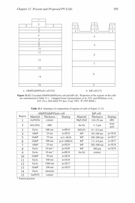
Chapter 11 Present and Proposed PV Cells 393
Table 11.1 Summary of composition of regions of cells of Figure 11.12.
AlInP/GaInP/GaAs cell InP cellRegion Material Thickness Doping Material Thickness Doping
1 Au/Ni/Ge contact MgF2/ZnS 110−55 nm ARC
2 SiO2/SiNx ARC Au-Ge 2−3 µmfrontgrid
3 GaAs 600 nm n=8E18 InGaAs 0.1−0.5 µm
4 AlInP 25 nm n=2E18 InP 50−100 nm p=1E18
5 GaInP 75 nm n=1−4E18 InP 100−200 nm p=1E17
6 GaInP 400 nm p=5−500E16 InP 1.5−4.0 µm n=1E17
7 AlInP 25 nm p=5E18 InP 250−500 nm n=1E18
8 GaAs 10 nm * p=1E20 InP 400 µm n>1E18
9 GaAs 10 nm * n=8E18 Au-Ge contact
10 GaInP 50 nm n=2E18
11 GaAs 100 nm n=1E18
12 GaAs 3500 nm p=1E17
13 GaInP 100 nm p=1E19
14 GaAs substrate
15 Au/Pt/Ti contact
* Tunnel junction
a. AlInP/GaInP/GaAs cell [16] b. InP cell [17]
C
Figure 11.12 Cascaded AlInP/GaInP/GaAs cell and InP cell. Properties of the regions of the cellsare summarized in Table 11.1. (Adapted from Lammasniemi, et al., 823, and Hoffman, et al.,
815, 1997. 1997 IEEE.)Proc 26th IEEE PV Spec Conf, .
Photovoltaic Systems Engineering394
GaAs cells remain expensive to fabricate and are thus used primarily forextraterrestrial applications and in concentrating systems.
11.3.4 Cell Performance
Cells fabricated with III-V elements are generally extraterrestrial quality. Inother words, they are expensive, but they are high-performance units. Efficien-cies in excess of 20% are common and efficiencies of cells fabricated on moreexpensive GaAs substrates have exceeded 34% [25].
An important feature of extraterrestrial quality cells is the need for them tobe radiation resistant. Cells are generally tested for their degradation resultingfrom exposure to healthy doses of 1 MeV or higher energy protons and elec-trons. Degradation is generally less than 20% for high exposure rates.
Extraterrestrial cells are sometimes exposed to temperature extremes, so thecells are also cycled between −170 and +96oC for as many as 1600 cycles. Thecells also need to pass a bending test, a contact integrity test, a humidity test anda high temperature vacuum test, in which the cells are tested at a temperatureabove 140oC in vacuum for 168 hours [26].
Fill factors in excess of 80% have been achieved for GaAs cells. Single cellopen-circuit voltages are generally between 0.8 and 0.9 V.
The design of stacked cells depends upon the air mass under which the de-vice is intended to operate. In order to ensure equal photon-generated current ineach absorption layer, layer thickness needs to be adjusted for the air mass underwhich operation is anticipated, because air masses do not attenuate the entirespectrum proportionately, as shown in Figure 2.2.
In par photons are available at this wavelength at AM0 than at AM1. Thus, for opera-tion at AM1, the absorber width would need to be increased to generate a photo-current comparable to that which a narrower layer would generate at AM0. Thisconsideration is particularly important when optimizing cell performance atAM0, but can also be relevant for cells designed for use in regions where expo-sures to AM 1.5 or AM 2.0 may occur for long periods of cell operation.
The bottom line is that III-V cells are excellent extraterrestrial performers,and it appears that continued research will improve performance, reduce massand reduce cost of the cells. Whether III-V cells will be able to compete withother technologies for terrestrial applications will depend on the degree of futureimprovements in all technologies. This mystery will likely unfold before theeyes of any reader born after the fabrication of the first commercial PV cell.
11.4 Copper Indium (Gallium) Diselenide Cells
11.4.1 Introduction
The first CIS PV cell was reported in 1974 by a group at Bell Laboratories[27]. Copper indium diselenide was chosen as a potential photovoltaic materialbecause of its attractive direct bandgap (1.0 eV), its very high optical absorption
Chapter 11 Present and Proposed PV Cells 395
coefficient and its potentially inexpensive preparation. Furthermore, the cellcomponents are available in adequate quantities and the manufacturing, deploy-ment and decommissioning of the technology fall within acceptable environ-mental constraints.
While current technology involves the use of Cd as a cell component, thetotal quantity is relatively small, and efforts are underway to identify alternate,less toxic, materials to replace the Cd. The challenge with CIS, as with otherthin film technologies, is to prepare a cell with appropriate electric field for col-lection of photon-generated, electron-hole pairs. Then ohmic contacts need tobe affixed, with the front contact being highly conducting, but transparent toincident photons. The final device structure must be stable and must be encap-sulated to ensure long module lifetime.
Unlike Si, which has been studied intensely for decades and is well-understood by the scientific community, the fundamentals of CIS are less well-understood. For example, energy bands in Si have been studied extensively anddetailed explanations are available in nearly any solid-state devices text. CIS,on the other hand, rarely receives mention. As basic research on the propertiesof CIS leads to increased understanding of the fundamental properties of thematerial, chances for significant device improvement will be enhanced.
Current estimates for large-scale production of CIS devices suggest the pos-sibility of producing devices for $1.00/watt or less [28]. Achieving these pro-duction costs requires improving cell efficiency as much as possible in order tolower area-related costs. Frames, glass, encapsulants, array mounts and some-times the cost of land itself all fall into this category.
11.4.2 Production of Pure Cell Components
Copper [29]Of all the elements used in the production of semiconductors, copper is
probably the most abundant. It is known from prehistoric times. It occasionallyoccurs in pure form in nature, but also occurs in many minerals, such as cuprite,malachite, azurite, chalcopyrite and bornite. The sulfides, oxides and carbonatesare the most important sources of Cu. The refining process involves smelting,leaching and electrolysis. Since Cu is used in so many applications, and isfound in so many locations in so many different compounds, many differentmethods of Cu refining have been developed. The reader is referred to reference[29] for examples.
Copper can be refined to semiconductor grade by electrolysis of a solution ofcopper sulfate and sulfuric acid. The anode is made of approximately 99% pureCu and the solution is maintained so that almost everything that plates out on thecathode is Cu. The chemical reactions at anode and cathode are
anode Cu → Cu2+ + 2e− (11.10a)cathode Cu2+ + 2e− → Cu (11.10b)

Photovoltaic Systems Engineering396
Although it appears that this process is exclusively moving Cu from anode tocathode, it is also moving elements such as oxygen, sulfur, arsenic, antimony,bismuth, lead, nickel, selenium, tellurium, gold and silver from anode into solu-tion. Oxygen is generally the most common impurity in the anode Cu, in theform of Cu2O. As the Cu2O moves into the solution, it reacts with the sulfuricacid to form CuSO4 and H2O along with Cu, which precipitates into the slimealong with most of the other elements from the anode which do not dissolve.This loses half the Cu to the slime, but the slime then can be reprocessed.
Only the silver will dissolve, but addition of HCl or NaCl to the solution willprecipitate the silver. Hence, only the CuSO4 is left in solution for migration tothe cathode, with the net result that the Cu plates out onto the cathode.
The slime thus contains compounds such as Cu2S, Cu2Se, Ag2S and Ag2Se,all of which may be of interest in further refining operations for recovery of anyof the other elements. In the meantime, the Cu on the cathode will be very pureif the solution is properly controlled.
Indium [30]Indium is most commonly found with zinc, but is also found with iron, lead
and copper ores. Little use was made of In until it was found to be useful incertain semiconductors. Most commercial In is now obtained from the fluedusts and residues from smelting lead and zinc. As late as 1924, less than anounce of pure In existed, even though it is rather widely scattered throughout theworld, albeit in very small concentrations in host minerals. The price of highlypure In is in the neighborhood of $100 per ounce.
Several means of extracting In from its natural states are available. In thepresence of lead and zinc, the material can be melted and treated with chlorinegas or other chlorine source. This removes the Zn and In as chlorides, providedthat the temperature is low enough to prevent evaporation of the In. The chlo-ride slag is then leached with dilute sulfuric acid, which causes the In to pre-cipitate along with Zn dust. The next step is to melt the In-Zn mixture and re-move the Zn with Cl.
Indium is refined to semiconductor grade by further physical or chemicalseparation techniques, such as zone refining and fractional distillation of liquidIn compounds.
Selenium [31]Selenium is a group VI element, and, as a result, is very similar to sulfur in
many of its chemical properties, which accounts for its common occurrence withCuS. In its natural form, it combines naturally with 16 other elements and is amajor component of 39 mineral species and a minor component of another 37mineral species. Since Se is always combined with other elements, such as S,there are no identified “reserves” of Se. Certain native plant species preferen-tially absorb Se, and are sometimes indicators of the presence of the element.Elemental Se is relatively nontoxic, but many Se compounds are very poison-ous. Selenium is recovered primarily from the anode muds from the refining of
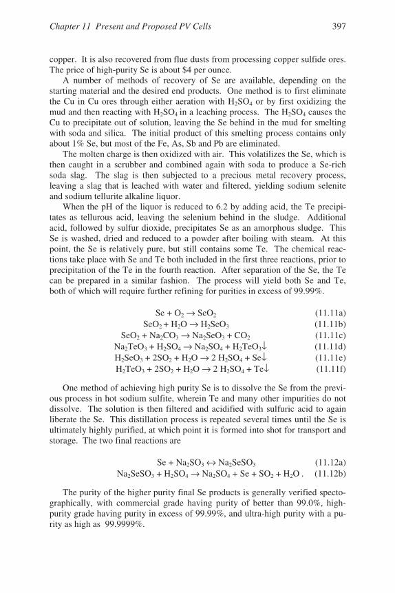
Chapter 11 Present and Proposed PV Cells 397
copper. It is also recovered from flue dusts from processing copper sulfide ores.The price of high-purity Se is about $4 per ounce.
A number of methods of recovery of Se are available, depending on thestarting material and the desired end products. One method is to first eliminatethe Cu in Cu ores through either aeration with H2SO4 or by first oxidizing themud and then reacting with H2SO4 in a leaching process. The H2SO4 causes theCu to precipitate out of solution, leaving the Se behind in the mud for smeltingwith soda and silica. The initial product of this smelting process contains onlyabout 1% Se, but most of the Fe, As, Sb and Pb are eliminated.
The molten charge is then oxidized with air. This volatilizes the Se, which isthen caught in a scrubber and combined again with soda to produce a Se-richsoda slag. The slag is then subjected to a precious metal recovery process,leaving a slag that is leached with water and filtered, yielding sodium seleniteand sodium tellurite alkaline liquor.
When the pH of the liquor is reduced to 6.2 by adding acid, the Te precipi-tates as tellurous acid, leaving the selenium behind in the sludge. Additionalacid, followed by sulfur dioxide, precipitates Se as an amorphous sludge. ThisSe is washed, dried and reduced to a powder after boiling with steam. At thispoint, the Se is relatively pure, but still contains some Te. The chemical reac-tions take place with Se and Te both included in the first three reactions, prior toprecipitation of the Te in the fourth reaction. After separation of the Se, the Tecan be prepared in a similar fashion. The process will yield both Se and Te,both of which will require further refining for purities in excess of 99.99%.
Se + O2 → SeO2 (11.11a)SeO2 + H2O → H2SeO3 (11.11b)
SeO2 + Na2CO3 → Na2SeO3 + CO2 (11.11c)Na2TeO3 + H2SO4 → Na2SO4 + H2TeO3↓ (11.11d)H2SeO3 + 2SO2 + H2O → 2 H2SO4 + Se↓ (11.11e)H2TeO3 + 2SO2 + H2O → 2 H2SO4 + Te↓ (11.11f)
One method of achieving high purity Se is to dissolve the Se from the previ-ous process in hot sodium sulfite, wherein Te and many other impurities do notdissolve. The solution is then filtered and acidified with sulfuric acid to againliberate the Se. This distillation process is repeated several times until the Se isultimately highly purified, at which point it is formed into shot for transport andstorage. The two final reactions are
Se + Na2SO3 ↔ Na2SeSO3 (11.12a)Na2SeSO3 + H2SO4 → Na2SO4 + Se + SO2 + H2O . (11.12b)
The purity of the higher purity final Se products is generally verified specto-graphically, with commercial grade having purity of better than 99.0%, high-purity grade having purity in excess of 99.99%, and ultra-high purity with a pu-rity as high as 99.9999%.
Photovoltaic Systems Engineering398
Cadmium [32]Cadmium was discovered in 1817 [20] by Friedrich Stromeyer in zinc car-
bonate and by K. S. L. Hermann in a specimen of zinc oxide. The common de-nominator is that cadmium is commonly found embedded in zinc compounds,although cadmium sulfide is found in Scotland, Bohemia and Pennsylvania.
Since zinc is routinely refined, the leftover cadmium from the process isgenerally recovered, mixed with carbon and redistilled to yield an enriched dust.This process is repeated several times. Then hydrochloric acid is mixed with thecadmium dust, and zinc is added, resulting in the precipitation of the cadmium.After several repetitions of this process, electrolysis is finally used to deposit thefinal material. Cadmium is a group II metallic element, and along with solutionsof its compounds, is highly toxic.
Sulfur [33]Sulfur is abundant in the crust of the earth, both in elemental and combined
forms. Elemental sulfur tends to occur in layers above salt domes. Abundantsupplies of elemental sulfur have been discovered in many locations around theworld. It has been used for thousands of years in many applications.
Elemental sulfur is generally recovered by pumping superheated water downa well to melt the sulfur, after which the molten sulfur is extracted from the well.The elemental sulfur is then generally reacted with a suitable element to enablethe sulfur to be carried in a gaseous state for vapor deposition onto a substrate.
Molybdenum [34]Molybdenum, a group VI metal, is an important metal for making ohmic
contacts, particularly as the back contact in a CIS cell. The metal was first pre-pared by P. J. Hjelm in 1782. It has high strength, high corrosion resistance andis often used in alloys, particularly in the production of stainless steel. It retainsits strength at high temperatures better than most other metals.
Most Mo is mined in the U.S., Canada and Chile. Molybdenum occurs prin-cipally in MoS2, but the concentration of MoS2 in ores is rather small. About aton of ore must be mined, crushed and milled to recover about 4 pounds of Mo.After the ore is crushed, the MoS2 is recovered in relatively high concentrationby floatation.
Roasting then drives off the sulfur and oxidizes the Mo to MoO3. Reductionwith H2 at high temperature yields Mo in powder form with purity in the 99%range. The powder can be reacted with halogens to form compounds such asMoF6 and MoCl5, which are suitable for vapor phase deposition of Mo.
11.4.3 Fabrication of the CIS Cell
While it is possible to produce both n-type and p-type CIS, homojunctions inthe material are neither stable nor efficient. A good junction can be made, how-ever, by creating a heterojunction with n-type CdS and p-type CIS.
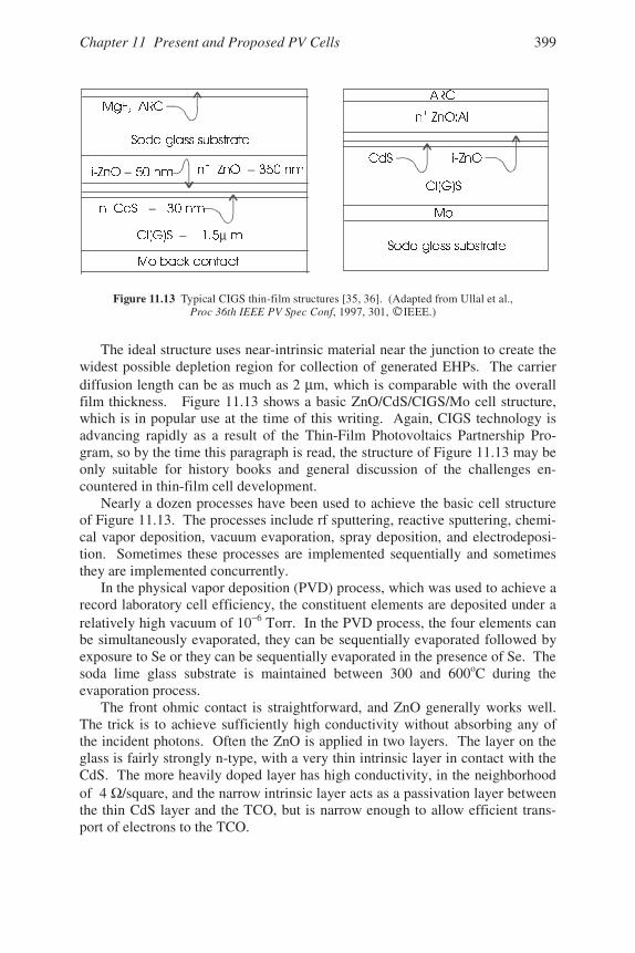
Chapter 11 Present and Proposed PV Cells 399
The ideal structure uses near-intrinsic material near the junction to create thewidest possible depletion region for collection of generated EHPs. The carrierdiffusion length can be as much as 2 µm, which is comparable with the overallfilm thickness. Figure 11.13 shows a basic ZnO/CdS/CIGS/Mo cell structure,which is in popular use at the time of this writing. Again, CIGS technology isadvancing rapidly as a result of the Thin-Film Photovoltaics Partnership Pro-gram, so by the time this paragraph is read, the structure of Figure 11.13 may beonly suitable for history books and general discussion of the challenges en-countered in thin-film cell development.
Nearly a dozen processes have been used to achieve the basic cell structureof Figure 11.13. The processes include rf sputtering, reactive sputtering, chemi-cal vapor deposition, vacuum evaporation, spray deposition, and electrodeposi-tion. Sometimes these processes are implemented sequentially and sometimesthey are implemented concurrently.
In the physical vapor deposition (PVD) process, which was used to achieve arecord laboratory cell efficiency, the constituent elements are deposited under arelatively high vacuum of 10−6 Torr. In the PVD process, the four elements canbe simultaneously evaporated, they can be sequentially evaporated followed byexposure to Se or they can be sequentially evaporated in the presence of Se. Thesoda lime glass substrate is maintained between 300 and 600oC during theevaporation process.
The front ohmic contact is straightforward, and ZnO generally works well.The trick is to achieve sufficiently high conductivity without absorbing any ofthe incident photons. Often the ZnO is applied in two layers. The layer on theglass is fairly strongly n-type, with a very thin intrinsic layer in contact with theCdS. The more heavily doped layer has high conductivity, in the neighborhoodof 4 Ω/square, and the narrow intrinsic layer acts as a passivation layer betweenthe thin CdS layer and the TCO, but is narrow enough to allow efficient trans-port of electrons to the TCO.
− −
−
− µ
!"!!
#
Figure 11.13 Typical CIGS thin-film structures [35, 36]. (Adapted from Ullal et al.,, 1997, 301, IEEE.)Proc 36th IEEE PV Spec Conf C
Photovoltaic Systems Engineering400
11.4.4 Cell Performance
When new technology PV cells are developed, normally small area cells arefabricated first to determine whether it appears practical to extend the technol-ogy to larger area cells and modules. At the time of this writing, the highestperformance achieved for a CIGS laboratory cell was 18.9% [25]. Scaling up tothe production of minimodules with areas up to 100 cm2 resulted in decrease inefficiency to 13% and further scaling up to 4 ft2 modules generally resulted inefficiencies less than 10%. In March, 1999, Siemens Solar reported a 3651 cm2
CIGSeS module with an efficiency confirmed by NREL of 12.1% [25].Clearly, the challenge in module development is to overcome the factors that
result in degradation of cell performance and clearly these challenges are beingundertaken ambitiously. To do so requires understanding of the factors thatcause the degradation. Some of these considerations include general device de-sign, contact grid design, antireflection coatings and the sheet resistance of win-dow layers.
An example of the trade-offs involved in scaling up a technology is the ZnOtransparent contact. For a laboratory scale device with an area of 1 cm2 or so,the ZnO layer can be relatively thin, with a sheet resistivity of 15 Ω/square,since the relatively small current from the cell will experience minimal voltagedrop through this contact. The thin window absorbs a minimal amount of inci-dent radiation so the CIS absorber layer can achieve maximum conversion effi-ciency. However, as the cell is made larger, the sheet resistance of the TCOmust be reduced to prevent voltage drop at the contact and corresponding degra-dation of fill factor and cell efficiency. The price paid for lower sheet resistanceis a greater amount of absorption of incident photons by the transparent contact.
Series connection of cells can also cause cell performance degradation. Fig-ure 11.14 shows how individual cells have been replaced by minimodules thatare monolithically connected. This monolithic connection process eliminatesthe need for separate fabrication processes for interconnecting cells.
After deposition of the Mo, it is scribed to separate adjacent cells, creatingcells with a length of about 4 ft and a width of a fraction of an inch. Next, afterdeposition of the CIS cell components, the CIS is scribed. Finally, after deposi-tion of the TCO, the TCO and CIS are scribed. While this process may appearto be straightforward, it can also be appreciated that the first cut needs to removeall of the Mo, but none of the glass. The second and third cuts must leave the!" c-ess falls somewhat short of being classified as trivial.
By incorporating Ga into the CIS mixture, the bandgap of the material can beincreased beyond 1.1 eV. This movement of the bandgap energy closer to thepeak of the solar spectrum increases conversion efficiency in this wavelengthregion and leaves lower energy photons for capture by the free carrier absorptionprocess in the transparent conducting oxide (TCO) layer while the higher energyphotons are converted to EHPs. The result is increasing the cell open-circuitvoltage from approximately 0.4 V to as high as 0.68 V, with fill factors ap-
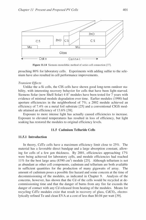
Chapter 11 Present and Proposed PV Cells 401
proaching 80% for laboratory cells. Experiments with adding sulfur to the sele-nium have also resulted in cell performance improvements.
Transient EffectsUnlike the a-Si cells, the CIS cells have shown good long-term outdoor sta-
bility, with interesting recovery behavior for cells that have been light-starved.Siemens Solar (now Shell Solar) 4 ft2 modules have been tested for 7 years withevidence of minimal module degradation over time. Earlier modules (1990) hadaperture efficiencies in the neighborhood of 7%; a 2002 module achieved anefficiency of 7.4% on a metal foil substrate [25] and a conventional CIGS mod-ule attained an efficiency of 13.6% [38].
Exposure to more intense light has actually caused efficiencies to increase.Exposure to elevated temperatures has resulted in loss of efficiency, but lightsoaking has restored the modules to original efficiency levels.
11.5 Cadmium Telluride Cells
11.5.1 Introduction
In theory, CdTe cells have a maximum efficiency limit close to 25%. Thematerial has a favorable direct bandgap and a large absorption constant, allow-ing for cells of a few µm thickness. By 2001, efficiencies approaching 17%were being achieved for laboratory cells, and module efficiencies had reached11% for the best large area (8390 cm2) module [25]. Although tellurium is notas abundant as other cell components, cadmium and tellurium are both availablein sufficient quantities for the production of many gigawatts of array. Theamount of cadmium poses a possible fire hazard and some concern at the time ofdecommissioning of the modules, as indicated in Chapter 9. Analysis of theconcerns, however, has shown that the Cd of the cells would be recycled at de-commissioning time and that the danger of burns from any fire far exceeds thedanger of contact with any Cd released from heating of the modules. Means forrecycling CdTe modules exist that result in recovery of glass, CdCO3, electro-lytically refined Te and clean EVA at a cost of less than $0.04 per watt [39].
Figure 11.14 Siemens monolithic method of series cell connection [37].
Photovoltaic Systems Engineering402
At the time of this writing, CdTe modules are undergoing large-scale testing,but are not yet commercially available. Progress toward commercialization israpid, and it is likely that by the time this paragraph is bound by a hard cover,commercial CdTe modules will be available. Purification of all of the compo-nents of the CdTe cell have been discussed so far except the Te. After a briefsummary of the extraction and purification of Te, cell fabrication and cell per-formance will be discussed.
11.5.2 Production of Pure Tellurium [33]
Tellurium is a group VI metallic element, which was discovered by Mullerin Transylvanian gold ore in 1782 and first extracted and identified by M. H.Klaproth in 1798. It is found as tellurides of copper, lead, silver, gold, iron andbismuth and is widely distributed over the surface of the earth, although its per-centage in the earth’s crust is very small. The primary sources of tellurium forproduction are leftovers from copper and lead refining, where tellurium and se-lenium both appear in very small quantities.
When copper is produced by electrolysis, the tellurium is precipitated alongwith other impurities in the copper to become a sludge at the anode. Severalalternative chemical means are then used to separate the tellurium from the otherimpurities in the sludge. The first step is to produce tellurium dioxide, whichprecipitates out of solution while the other impurities remain dissolved. Alter-natively, other impurities may first be precipitated, leaving behind higher con-centrations of tellurium in the form of tellurous acid. If the oxide is produced,then the oxide is reduced to form elemental tellurium.
Elemental tellurium remains contaminated with iron, copper, tin, silver, lead,antimony and bismuth and can be further purified by low pressure distillation,where the heavier metals remain in the residue. Selenium, however, is volatileand remains a contaminant in the distilled tellurium. Further purification can beachieved by dissolving the tellurium in strong nitric acid. Diluting and boilinghydrolyzes the tellurium to a precipitate form. The precipitate is separated,washed, dissolved in hydrochloric acid and reduced with sulfur dioxide.
This relatively pure tellurium can be brought to the ultrahigh purity state byzone refining in an inert gas atmosphere, and single crystals can be grown byeither the Czochralski or Bridgman methods.
Tellurium is classified as “probably” toxic and reasonable care is recom-mended in its handling.
11.5.3 Production of the CdTe Cell
Figure 11.15 shows a typical CdTe cell structure. The cell begins with aglass superstrate with a transparent, conducting, oxide layer about 1 µm thick, athin CdS buffer layer about 0.1 µm thick, a CdTe layer a few µm thick and arear contact of Au, Cu/Au, Ni, Ni/Al, ZnTe:Cu or (Cu, HgTe).
The TCO layer has been fabricated with SnO, InSnO and Cd2SnO4. The

Chapter 11 Present and Proposed PV Cells 403
Cd2SnO4 has been shown to exhibit better conductivity and better transparency[40] than the other TCOs and may end up as the preferred TCO. The Cd2SnO4
layer is deposited by combining CdO and SnO2 in a 2:1 proportion in a targetmaterial, which is then deposited by means of radio frequency magnetron sput-tering onto the glass superstrate.
The thin n-type CdS layer has been deposited by the metal organic chemicalvapor deposit (MOCVD) process as well as by other thin film deposition tech-niques. The layer needs to be annealed prior to deposition of the CdTe in orderto reduce CdS surface roughness, thus reducing defects on the CdS/CdTeboundary. This is normally accomplished in air at approximately 400oC forabout 20 minutes.
An interesting challenge exists with regard to the CdS layer, since the layeris so thin. During deposition of the CdTe or subsequent heat treatment of thecell, intermixing of the CdS and CdTe can occur at the boundary. This can re-sult in junctions between the CdTe and the TCO layer, which causes significantreductions in cell open-circuit voltage. Several methods of minimizing thismixing have been proposed [41].
Numerous methods have been used to deposit the CdTe layer, including at-mospheric pressure chemical vapor deposition (APCVD), atomic layer epitaxy(ALE), close-spaced sublimation (CSS), electrodeposition (ED), laser ablation,physical vapor deposition (PVD), screen printing (SP), spray, sputtering andMOCVD [25]. The CdTe layer is subjected to a heat treatment in the presenceof CdCl2 for about 20 minutes at about 420oC. This treatment enhances graingrowth in the CdTe layer to reduce grain boundary trapping effects on minoritycarriers. Nonheat-treated CdTe cells tend to have open-circuit voltages less than0.5 V, while after heat treating, VOC can exceed 0.8 V.
Another important step in optimizing cell performance is to ensure stabilityof the back contact. Before the back contact is applied, the CdTe is etched withnitric-phosphoric (NP), resulting in a layer of elemental Te at the back CdTesurface. The elemental Te produces a more stable contact between the p-typeCdTe and the back metal [42].
C
Figure 11.15 Basic structure of a CdTe PV cell [35]. (Adapted from Ullal et al.,1997, 301, 1997 IEEE.)Proc 26th IEEE PV Spec Conf,
Photovoltaic Systems Engineering404
Final processing of modules involves encapsulation of the back of the cellwith a layer of EVA between the metallization and another layer of glass.
11.5.4 Cell Performance
No fewer than nine companies have shown an interest in commercial appli-cations of CdTe. As of 2001, depending on the fabrication methodology, effi-ciencies of close to 17% had been achieved for small area cells (≈1 cm2), and11% on a module with an area of 8390 cm2 [25]. Sufficient experience has beenlogged with large-scale production to identify areas in which improvement isneeded [43]. These areas include improving the design, operation and control ofa CdTe reactor; increasing the understanding of the fundamental properties ofCdTe films; maintaining uniformity of materials and device properties overlarge areas, including the interdiffusion of CdTe and CdS and the back contact;obtaining stability of the back contact and addressing any environmental con-cerns over Cd. Since Te availability may limit cell production, increasing per-formance with thinner layers of CdTe is also desirable. Reducing the thicknessof the "#$ %o-vided that efficiency can be maintained or increased. Just as in the case of otherthin-film arrays, area-related costs limit the minimal cost per watt of CeTe ar-rays, so increase in efficiency is important to minimize cost per watt.
Fill factors for lab cells have been obtained in the 65- to-75% range [44],with the slope of the cell J-V curve at VOC in the range of 5 Ω-cm2. Short-circuitcurrent densities upward from 25 mA/cm2 have been obtained by using a thinbuffer layer of CdS along with a thin insulating TCO layer between the heavilydoped TCO and the CdS layer [25].
Experimental CdTe arrays in sizes up to 25 kW have been deployed in Cali-fornia, Ohio, Tunisia, Colorado and Florida for testing purposes [25]. Two 25kW arrays are in use at Edwards Air Force Base in California as a power sourcefor electrolysis of water to provide H2 for fuel cells. Two 10 kW arrays are con-nected to utility grids and are reported to be performing very well. No degrada-tion has been observed for the first 2 years of operation.
11.6 Emerging Technologies
11.6.1 New Developments in Silicon Technology
While progress continues on conventional Si technology, new ideas are alsobeing pursued for crystalline and amorphous Si cells. The goal of Si technologyhas been to maintain good transport properties, while improving photon absorp-tion and reducing the material processing cost of the cells. When the thicknessof Si is reduced, some sort of substrate material is required to maintain sufficientphysical strength for the cell. Two substrates that seem to show promise areceramic and graphite, both having led to cell efficiencies in the 10% range [45].Diffusion of contaminants such as Mg, Mn and Fe from ceramic substrates hasbeen shown to limit performance of Si on ceramics, and methods of introducing
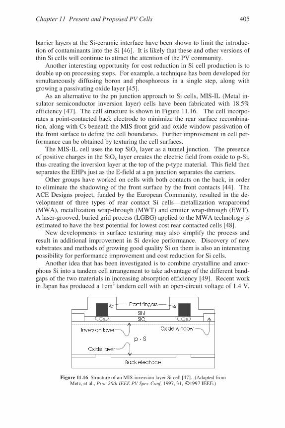
Chapter 11 Present and Proposed PV Cells 405
barrier layers at the Si-ceramic interface have been shown to limit the introduc-tion of contaminants into the Si [46]. It is likely that these and other versions ofthin Si cells will continue to attract the attention of the PV community.
Another interesting opportunity for cost reduction in Si cell production is todouble up on processing steps. For example, a technique has been developed forsimultaneously diffusing boron and phosphorous in a single step, along withgrowing a passivating oxide layer [45].
As an alternative to the pn junction approach to Si cells, MIS-IL (Metal in-sulator semiconductor inversion layer) cells have been fabricated with 18.5%efficiency [47]. The cell structure is shown in Figure 11.16. The cell incorpo-rates a point-contacted back electrode to minimize the rear surface recombina-tion, along with Cs beneath the MIS front grid and oxide window passivation ofthe front surface to define the cell boundaries. Further improvement in cell per-formance can be obtained by texturing the cell surfaces.
The MIS-IL cell uses the top SiOx layer as a tunnel junction. The presenceof positive charges in the SiOx layer creates the electric field from oxide to p-Si,thus creating the inversion layer at the top of the p-type material. This field thenseparates the EHPs just as the E-field at a pn junction separates the carriers.
Other groups have worked on cells with both contacts on the back, in orderto eliminate the shadowing of the front surface by the front contacts [44]. TheACE Designs project, funded by the European Community, resulted in the de-velopment of three types of rear contact Si cells—metallization wraparound(MWA), metallization wrap-through (MWT) and emitter wrap-through (EWT).A laser-grooved, buried grid process (LGBG) applied to the MWA technology isestimated to have the best potential for lowest cost rear contacted cells [48].
New developments in surface texturing may also simplify the process andresult in additional improvement in Si device performance. Discovery of newsubstrates and methods of growing good quality Si on them is also an interestingpossibility for performance improvement and cost reduction for Si cells.
Another idea that has been investigated is to combine crystalline and amor-phous Si into a tandem cell arrangement to take advantage of the different band-gaps of the two materials in increasing absorption efficiency [49]. Recent workin Japan has produced a 1cm2 tandem cell with an open-circuit voltage of 1.4 V,
C
Figure 11.16 Structure of an MIS-inversion layer Si cell [47]. (Adapted fromMetz, et al., 1997, 31, 1997 IEEE.)Proc 26th IEEE PV Spec Conf,
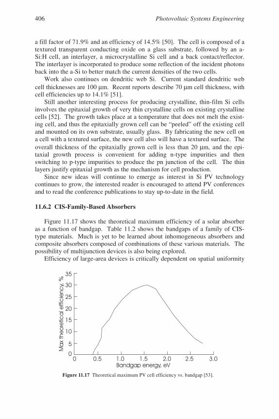
Photovoltaic Systems Engineering406
a fill factor of 71.9% and an efficiency of 14.5% [50]. The cell is composed of atextured transparent conducting oxide on a glass substrate, followed by an a-Si:H cell, an interlayer, a microcrystalline Si cell and a back contact/reflector.The interlayer is incorporated to produce some reflection of the incident photonsback into the a-Si to better match the current densities of the two cells.
Work also continues on dendritic web Si. Current standard dendritic webcell thicknesses are 100 µm. Recent reports describe 70 µm cell thickness, withcell efficiencies up to 14.1% [51].
Still another interesting process for producing crystalline, thin-film Si cellsinvolves the epitaxial growth of very thin crystalline cells on existing crystallinecells [52]. The growth takes place at a temperature that does not melt the exist-ing cell, and thus the epitaxially grown cell can be “peeled” off the existing celland mounted on its own substrate, usually glass. By fabricating the new cell ona cell with a textured surface, the new cell also will have a textured surface. Theoverall thickness of the epitaxially grown cell is less than 20 µm, and the epi-taxial growth process is convenient for adding n-type impurities and thenswitching to p-type impurities to produce the pn junction of the cell. The thinlayers justify epitaxial growth as the mechanism for cell production.
Since new ideas will continue to emerge as interest in Si PV technologycontinues to grow, the interested reader is encouraged to attend PV conferencesand to read the conference publications to stay up-to-date in the field.
11.6.2 CIS-Family-Based Absorbers
Figure 11.17 shows the theoretical maximum efficiency of a solar absorberas a function of bandgap. Table 11.2 shows the bandgaps of a family of CIS-type materials. Much is yet to be learned about inhomogeneous absorbers andcomposite absorbers composed of combinations of these various materials. Thepossibility of multijunction devices is also being explored.
Efficiency of large-area devices is critically dependent on spatial uniformity
Figure 11.17 Theoretical maximum PV cell efficiency vs. bandgap [53].
Chapter 11 Present and Proposed PV Cells 407
of the absorber layers and electrodes as well as on the performance of cell inter-connects. Hence, with any of the listed absorber possibilities, the key to per-formance will be in the engineering of reliable and reproducible module pro-cessing techniques.
Even an issue as mundane as the quality and cleanliness of the glass sub-strate can have a significant effect on module performance. Polishing the glasswith CeO2 has been shown to increase module performance [54]. Furthermore, itappears that if a certain amount of Na diffuses from the glass to the absorber,the absorber performance is increased [53].
Table 11.2 Bandgaps of CIS-related materials [54].
Material BandgapCuInSe2 1.05 eVAgInSe2 1.24 eVCuInS2 1.56 eV
CuGaSe2 1.67 eVAgGaSe2 1.69 eVAgInS2 1.95 eVCuGaS2 2.33 eVAgGaS2 2.56 eV
Meanwhile, work is underway to reduce the material usage in the productionof CIS modules in order to further reduce production costs. Examples of reduc-tion of material use include halving the width of the Mo contact layer, reductionin the use of H2S and H2Se and a reduction in ZnO, provided that a minimumthickness can be maintained [55].
11.6.3 Other III-V and II-VI Emerging Technologies
It appears that compound tandem cells will receive appreciable emphasis inthe III-V family of cells over the next few years. For example,Ga0.84In0.16As0.68P0.32 , lattice matched to GaAs, has a bandgap of 1.55 eV andmay prove to be an ideal material for use under AM0 conditions, since it alsohas good radiation resistance [56]. Cells have been fabricated with Al0.51In0.49Pand Ga0.51In0.49P window layers, with the best 1 cm2 cell having an efficiency ofjust over 16%, but having a fill factor of 85.4%. The best performing windowwas the AlInP.
Mechanical stacking of materials having different lattice constants has alsobeen proposed [57]. Performance modeling of a proposed 26-layer, 4-junctiondevice based on GaInP, GaAs, GaInAsP and GaInAs has shown the possibilityof 35.3% conversion efficiency.
Cell efficiencies can be increased by concentrating sunlight on the cells.Although the homojunction cell efficiency limit under concentration is just un-der 40%, quantum well (QW) cells have been proposed to increase the concen-trated efficiency beyond the 40% level [58]. In QW cells, intermediate energy
Photovoltaic Systems Engineering408
levels are introduced between the host semiconductor’s valence and conductionbands to permit absorption of lower energy photons. These levels must be cho-sen carefully so they will not act as recombination centers, however, or the gainsof EHPs from lower energy incident photons will be lost to the recombinationprocesses. Laboratory cells have shown higher VOC resulting from a decrease indark current for these cells. Intense study is underway with the goal of under-standing the electronic processes that take place within these cells [59].
11.6.4 Other Technologies
Thermophotovoltaic CellsTo this point, discussion has been limited to the conversion of visible and
near infrared spectrum to EHPs. The reason is simply that the solar spectrumpeaks out in the visible range. However, heat sources and incandescent lightsources produce radiation in the longer infrared regions, and in some instances,it is convenient to harness radiated heat from these processes by converting it toelectricity. This means using semiconductors with smaller bandgaps, such asGe. More exotic structures, such as InAsSbP, with a bandgap of 0.45-0.48 eVhave also been fabricated. The InAsSbP can be fabricated as p-type and n-type.The pn junction is grown on a substrate of InAs [60].
Intermediate Band Solar CellsIn all cells described to this point, absorption of a photon has resulted in the
generation of a single EHP. If an intermediate band material is sandwichedbetween two ordinary semiconductors, it appears that it may be possible for thematerial to absorb two photons of relatively low energy to produce a single EHPat the combined energies of the two lower energy photons. The first photonraises an electron from the valence band to the intermediate level, creating ahole in the valence band, and the second photon raises the electron from the in-termediate level to the conduction band. The trick is to find such an intermedi-ate band material that will “hold” the electron until another photon of the appro-priate energy impinges upon the material. Such a material should have half itsstates filled with electrons and half empty in order to optimally accommodatethis electron transfer process. It appears that III-V compounds may be the bestcandidates for implementation of this technology. Theoretical maximum effi-ciency of such a cell is 63.2% [61].
Supertandem Cells If a large number of cells are stacked with the largest bandgap on top and
the bandgap of subsequent cells decreasing, the theoretical maximum efficiencyis 86.8% [62]. A 1 cm2 4-junction cell has been fabricated with an efficiency of35.4%. The maximum theoretical efficiency of this cell is 41.6% [63]. Perhapsone day one of the readers of this paragraph (or one of their great-great grand-children) will fabricate a cell with the maximum theoretical efficiency.
Chapter 11 Present and Proposed PV Cells 409
Hot Carrier CellsThe primary loss mechanism in PVcells is the energy lost in the form of heat
when an electron is excited to a state above the bottom of the conduction bandof a PV cell by a photon with energy greater than the bandgap. The electronwill normally drop to the lowest energy available state in the conduction band,with the energy lost in the process being converted to heat. Hence, if this lossmechanism can be overcome, the efficiency of a cell with a single junctionshould be capable of approaching that of a supertandem cell. One method ofpreventing the release of this heat energy by the electron is to heat the cell, sothe electron will remain at the higher energy state. The process is called ther-moelectronics and is currently being investigated [62].
Optical Up-and Down-ConversionAn alternative to varying the electrical bandgap of a material is to reshape
the energies of the incident photon flux. Certain materials have been shown tobe capable of absorbing two photons of two different energies and subsequentlyemitting a photon of the combined energy. Other materials have been shown tobe capable of absorbing a single high-energy photon and emitting two lowerenergy photons. These phenomena are similar to up-conversion and down-con-version in communications circuits at radio frequencies.
By the use of both types of materials, the spectrum incident on a PV cell canbe effectively narrowed to a range that will result in more efficient absorption inthe PV cell. An advantage of this process is that the optical up-and-down con-verters need not be a part of the PV cell. They simply need to be placed be-tween the photon source and the PV cell. In tandem cells, the down-converterwould be placed ahead of the top cell and the up-converter would be integratedinto the cell structure just ahead of the bottom cell.
Organic PV CellsEven more exotic than any of the previously mentioned cells is the organic
cell. In the organic cell, electrons and holes are not immediately formed as thephoton is absorbed. Instead, the incident photon creates an exciton, which is abound EHP. In order to free the charges, the exciton binding energy must beovercome. This dissociation occurs at the interface between materials of highelectron affinity and low ionization potential [63]. Photoluminescence is relatedto this process. Just to end this chapter with a little chemistry, the reader willcertainly want to know that one material that is a candidate for organic PV hap-pens to be poly2,5-dimethoxy-1,4-phenylene-1,2-ethenylene-2-methoxy-5-(2-ethyl-hexyloxy)-1,4-phenylene-1,2-ethenylene, which goes by the nicknameM3EH-PPV. Whether M3EH-PPV will dominate the PV market one day re-mains to be seen. So far efficiencies of this very challenging technology havebeen in the 1% range.
Photovoltaic Systems Engineering410
11.6.5 Summary
Regardless of the technology or technologies that may result in low-cost,high-performance PV cells, it must be recognized that the life cycle cost of a celldepends on the cell’s having the longest possible, maintenance-free lifetime.Thus, along with the developments of new technologies for absorbers, develop-ment of reliable encapsulants and packaging for the modules will also meritcontinued research and development activity.
Every year engineers make improvements on products that have been in ex-istence for many years. Automobiles, airplanes, electronic equipment, buildingmaterials and many more common items see improvement every year. Even theyo-yo, a popular children’s toy during the 1940s and 1950s, came back withbetter-performing models. Hence, it should come as no surprise to the engineerto see significant improvements and scientific breakthroughs in the PV industrywell into the next millennium. The years ahead promise exciting times for theengineers and scientists working on the development of new photovoltaic celland system technologies.
Problems
11.1. Assume a PV module is to have dimensions of 1 ft x 4 ft. Also assumethat 4-inch round cells are available.a. Calculate the percentage of the module area that will be covered with
circular cells.b. Assume 6-inch diameter cells are available so they can have their edges
sawed to produce cells that are 4 inches across. Calculatethe percentage fill of these “squared up” cells.
c. What is the percentage loss of material in the “squaring up” process?d. Repeat b and c for 5-inch diameter cells.
11.2. Determine the expression for the depth of the junction after the drive-indiffusion step.
11.3. Sketch the impurity distribution profile between the junction and the backcontact of a single crystal silicon cell to show how the annealed aluminumof the back contact creates an accelerating E-field.
11.4. What volume and weight of tellurium is needed to produce a square meter "# $ &'"#oc-cupy equal volumes within the film.
Chapter 11 Present and Proposed PV Cells 411
11.5. What volume and weight of indium is required to fabricate a 1 MW PVCIS array if the CIS layer thickness is 1.5 µm, assuming that 18% of thelayer volume is due to the In. Assume an array efficiency of 10% andstandard test conditions.
References
[1] Ullal, H., et al., Proc. 29th IEEE PV Spec. Conf., 2002, 472−477 . [2] Tarrant, D. E. and Gay, R. R., Research on High Efficiency, Large Area CuInSe2 -
Based Thin Film Modules, Final Technical Report, NREL, Golden, CO, April 1995. [3] http://www.eia.gov/pub/international/ (Worldwide electrical generation capacity
data.) [4] Markvart, T., Ed., Solar Electricity, John Wiley & Sons, Chichester, U.K., 1994.
[5] Ciszek, T. F., Proc. 20th IEEE PV Spec Conf., 1988, 31. [6] Streetman, B. G., Solid State Electronic Devices, 4th Ed., Prentice Hall, Englewood
Cliffs, NJ, 1995. [7] Bohland, J., Accelerated aging of PV encapsulants by high intensity UV exposure,
Proc. 1998 Photovoltaic Performance and Reliability Workshop, Cocoa Beach, FL,November 3−5, 1998.
[8] www.ase-international.com (For information on EFG process) [9] Rosenblum, A.E., et al., Proc. 29th IEEE PV Spec. Conf., 2002, 58−61.[10] Hanoka, J. I., Proc. 29th IEEE PV Spec. Conf., 2002, 66−69.[11] Green, M. A. and Wenham, S. R., Novel parallel multijunction solar cell, Applied
Physics Letters 65, 1994, 2907.[12] Green, M. A., Proc. 29th IEEE PV Spec. Conf., 2002, 9−14.[13] DelleDonne, E., et al., Proc. 29th IEEE PV Spec. Conf., 2002, 82−85.[14] Basore, Paul A., Proc. 29th IEEE PV Spec. Conf., 2002, 49−52.[15] Brendel, R., et al., Proc. 29th IEEE PV Spec. Conf., 2002, 86−89.[16] Guha, S., Yang, J., et al., Proc. 26th IEEE PV Spec. Conf., 1997, 607−610.[17] Huang, J., Lee, Y., et al., Proc. 26th IEEE PV Spec. Conf., 1997, 699−702.[18] Guha, S., and Yang, J., Proc. 29th IEEE PV Spec. Conf., 2002, 1070−1075.[19] Yang, J., Banerjee, A., et al., Proc. 26th IEEE PV Spec. Conf., 1997, 563−568.[20] Standen, A., Executive Ed., Kirk-Othmer Encyclopedia of Chemical Technology,
2nd Ed., Vol 10, John Wiley & Sons, New York, 1968.[21] Standen, A., Executive Ed., Kirk-Othmer Encyclopedia of Chemical Technology,
2nd Ed., Vol 2, John Wiley & Sons, New York, 1968.[22] Williams, R., Modern GaAs Processing Methods, Artech House, Norwood, MA,
1990.[23] Lammasniemi, J., et al., Proc. 26th IEEE PV Spec. Conf., 1997, 823−826.[24] Hoffman, R., et al., Proc. 26th IEEE PV Spec. Conf., 1997, 815−818.[25] Kazmerski, L. L., Proc. 29th IEEE PV Spec. Conf., 2002, 21−27.[26] Brown, M. R., et al., Proc. 26th IEEE PV Spec. Conf., 1997, 805−810.[27] Shay, J. L., Wagner, S., and Kasper, H. M., Applied Physics Letters, 27, No. 2,
1975, 89.
Photovoltaic Systems Engineering412
[28] Wiedeman, S., et al., Proc. 14th NREL PV Program Review, AIP Conf. Proceedings394, Lakewood, CO, 1996, 133−142 .
[29] Standen, A., Executive Ed., Kirk-Othmer Encyclopedia of Chemical Technology,2nd Ed., Vol 6, John Wiley & Sons, New York , 1968.
[30] Standen, A., Executive Ed., Kirk-Othmer Encyclopedia of Chemical Technology,2nd Ed., Vol 11, John Wiley & Sons, New York, 1968.
[31] Standen, A., Executive Ed., Kirk-Othmer Encyclopedia of Chemical Technology,2nd Ed., Vol 17, John Wiley & Sons, New York, 1968.
[32] The Encyclopedia Brittanica, 15th ed., Encyclopedia Brittanica, Inc., Chicago, IL,1997.
[33] Standen, A., Executive Ed., Kirk-Othmer Encyclopedia of Chemical Technology,2nd Ed., Vol 19, John Wiley & Sons, New York , 1968.
[34] Standen, A., Executive Ed., Kirk-Othmer Encyclopedia of Chemical Technology,2nd Ed., Vol 13, John Wiley & Sons, New York, 1968.
[35] Ullal, H. S., Zweibel, K. and von Roedern, B., Proc. 26th IEEE PV Spec. Conf.,1997, 301−305.
[36] Carlson, D. E., et al., Proc. 25th IEEE PV Spec. Conf, 1996, 1023−1028.[37] Tarrant, D. E. and Gay, R. R., Thin-Film Photovoltaic Partnership Program⎯CIS-
based thin film PV Technology. Phase 2 Technical Report, October 1996-October1997, NREL report NREL/SR-520-24751, Golden, CO, May 1998.
[38] Konagai, M., Proc. 29th IEEE PV Spec. Conf., 2002, 38−43.[39] Bohland, J., et al., Proc. 26th IEEE PV Spec. Conf., 1997, 355−358.[40] Wu, X., Sheldon, P., et. al, Proc. 26th IEEE PV Spec. Conf., 1997, 347−350.[41] McCandless, B. E. and Birkmire, R. W., Proc 26th IEEE PV Spec. Conf., 1997,
307−312.[42] Levi, D. H., et al., Proc. 26th IEEE PV Spec. Conf., 1997, 351−354.[43] Birkmire, R. W., Proc. 26th IEEE PV Spec. Conf., 1997, 295−300.[44] Zhou, C. Z., et al., Proc. 26th IEEE PV Spec. Conf., 1997, 287−290.[45] Krygowski, T., Rohatgi, A., and Ruby, D., Proc 26th IEEE PV Spec. Conf., 1997,
19−24.[46] Slaoui, A., et al., Proc. 29th IEEE PV Spec. Conf., 2002, 90−93.[47] Metz, A., et al., Proc. 26th IEEE PV Spec. Conf., 1997, 31−34.[48] Schönecker, A., et al., Proc. 29th IEEE PV Spec. Conf., 2002, 106−109.[49] Kuznicki, Z. T., Proc. 26th IEEE PV Spec. Conf., 1997, 291−294.[50] Yamamoto, K., et al., Proc. 29th IEEE PV Spec. Conf., 2002, 1110−1113.[51] Meier, D. L., et al., Proc. 29th IEEE PV Spec. Conf., 2002, 110−113.[52] Brendel, R., et al., Proc. 29th IEEE PV Spec. Conf., 2002, 86−89.[53] Granata, J., Sites, J. R. and Tuttle, J. R., Proc. 14th NREL PV Program Review, AIP
Conf. Proceedings 394, Lakewood, CO, 1996, 621−630.[54] Tarrant, D. E. and Gay, R. R., Research on High Efficiency, Large Area CuInSe2
Modules, Final Technical Report, NREL, Golden, CO, April 1995.[55] Weiting, R., Proc. 29th IEEE PV Spec. Conf., 2002, 478−483.[56] Jaakkola, R., et al., Proc. 26th IEEE PV Spec. Conf., 1997, 891−894.[57] Sharps, P. R., et al., Proc. 26th IEEE PV Spec. Conf., 1997, 895−898.[58] Barnham, K. W. J. and Duggan, G., A new approach to high-efficiency multi-band-
gap solar cells, J. Appl. Phys. 67, 1990, 3490−3493.[59] Corkish, R. and Honsberg, C., Proc. 26th IEEE PV Spec. Conf., 1997, 923−926.[60] Khvostikov, V. P., et al., Proc. 29th IEEE PV Spec. Conf., 2002, 943−946.[61] Luque, A., et al., Proc. 29th IEEE PV Spec. Conf., 2002, 1190−1193.

Chapter 11 Present and Proposed PV Cells 413
[62] Green, M. A., Proc. 29th IEEE PV Spec. Conf., 2002, 1330−1334.[63] Zahler, J. M., et al., Proc. 29th IEEE PV Spec. Conf., 2002, 1029−1032.
Suggested Reading
Brown, K. E., et al., Proc. 29th IEEE PV Spec. Conf., 2002, 1186−1189.Goetzberger, A., Proc. 26th IEEE PV Spec. Conf., 1997, 1−6.Hu, C. and White, R. M., Solar Cells, From Basic to Advanced Systems, McGraw-
Hill, New York , 1983.Mahan, A. H., et al., Proc. 14th NREL PV Program Review, AIP Conf. Proceedings
394, Lakewood, CO, 1996, 27−32.Tuttle, J.R., et al., Proc. 14th NREL PV Program Review, AIP Conf. Proceedings
394, Lakewood, CO, 1996, 83−105.Weast, R. C., Ed-in-Chief; Lide, D. R., Ed.; Astle, M. J., Assoc. Ed.; Beyer, W. H.,
Assoc. Ed.; CRC Handbook of Chemistry and Physics, 70th Ed., CRC Press,Boca Raton, FL, 1990.


415
Appendix AAVERAGE DAILY IRRADIATION
FOR SELECTED CITIES
The U. S. data in the following tables has been compiled by the NationalRenewable Energy Laboratory. Data outside the U. S. has been compiled bySandia National Laboratories. Average daily irradiation in kWh/m2 is tabulatedfor each month of the year, including annual averages, for an assortment oforientations, including:
1. Fixed, south-facing arrays tilted at latitude −15o, latitude and latitude +15o.2. Single axis east-west tracking mounts tilted at three angles.3. Horizontal and vertical mounts (U. S. data only).4. Double axis tracking mounts.
The following cities are included, listed alphabetically by state, then bycountry. For 34 additional listings, the reader is encouraged to consult StandAlone Photovoltaic Systems, A Handbook of Recommended Design Practices, bySandia National Laboratories, Albuquerque, New Mexico. Appendix B lists theNREL and several other web sites that provide irradiation information.
1. Fairbanks, Alaska 2. Sacramento, California 3. Denver, Colorado 4. Miami, Florida 5. Atlanta, Georgia 6. Boston, Massachusetts 7. Albuquerque, New Mexico 8. Bismarck, North Dakota 9. Austin, Texas10. Seattle, Washington11. Luanda, Angola12. Buenos Aires, Argentina13. Melbourne, Australia14. Shanghai, Peoples Republic of China15. Paris-St. Maur, France16. New Delhi, India17. Tokyo, Japan18. Nairobi, Kenya19. Mexico D. F., Mexico20. Stockholm, Sweden

Photovoltaic Systems Engineering416
Avg 3.4
4.6
3.3
4.5
3.1
4.4
2.5
2.8
4.7
Dec 0.2
0.2
0.3
0.3
0.3
0.3
0.0
0.3
0.3
Nov 1.0
1.1
1.1
1.2
1.1
1.2
0.3
1.1
1.2
Oct
1.9
2.2
2.0
2.3
2.0
2.3
1.0
2.0
2.3
Sep
3.4
4.4
3.4
4.4
3.2
4.2
2.3
3.0
4.4
Aug 4.5
6.0
4.2
5.8
3.8
5.5
3.7
3.3
6.0
Jul
5.4
7.6
4.9
7.4
4.3
6.9
5.1
3.7
7.9
Jun
5.7
8.3
5.2
8.0
4.5
7.6
5.6
3.9
8.7
May
5.7
8.2
5.3
8.0
4.6
7.6
5.1
4.1
8.4
Apr
5.6
7.7
5.6
7.7
5.3
7.4
4.0
4.9
7.7
Mar
4.5
5.7
4.7
5.9
4.7
5.8
2.3
4.5
5.8
Feb
2.2
2.6
2.4
2.7
2.5
2.8
0.8
2.5
2.8
Jan
0.7
0.7
0.7
0.8
0.8
0.8
0.1
0.8
0.8
Fixe
dA
rray
1-A
xis
Tra
cker
Fixe
dA
rray
1-A
xis
Tra
cker
Fixe
dA
rray
1-A
xis
Tra
cker
Fai
rban
ks, A
K A
vera
ge D
aily
Pea
k Su
n H
ours
, kW
h/m
2
Lat
itude
: 64
°49
°52
Mon
th
Arr
ay ti
lted
at L
atitu
de−1
5°
Arr
ay ti
lted
at L
atitu
de
Arr
ay ti
lted
at L
atitu
de+1
5 °
Hor
izon
tal A
rray
Ver
tical
Sou
th-f
acin
gA
rray
2-A
xis
Tra
ckin
g A
rray
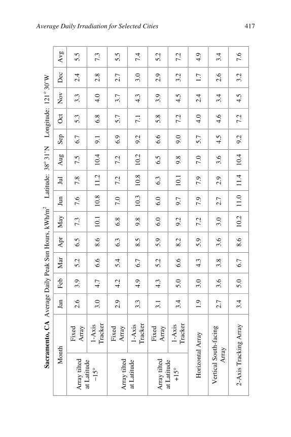
Average Daily Irradiation for Selected Cities 417
Avg 5.5
7.3
5.5
7.4
5.2
7.2
4.9
3.4
7.6
Dec 2.4
2.8
2.7
3.0
2.9
3.2
1.7
2.6
3.2
Nov 3.3
4.0
3.7
4.3
3.9
4.5
2.4
3.4
4.5
Oct
5.3
6.8
5.7
7.1
5.8
7.2
4.0
4.6
7.2
Sep
6.7
9.1
6.9
9.2
6.6
9.0
5.7
4.5
9.2
Aug 7.5
10.4
7.2
10.2
6.5
9.8
7.0
3.6
10.4
Jul
7.8
11.2
7.2
10.8
6.3
10.1
7.9
2.9
11.4
Jun
7.6
10.8
7.0
10.3
6.0
9.7
7.9
2.7
11.0
May
7.3
10.1
6.8
9.8
6.0
9.2
7.2
3.0
10.2
Apr
6.5
8.6
6.3
8.5
5.9
8.2
5.9
3.6
8.6
Mar
5.2
6.6
5.4
6.7
5.2
6.6
4.3
3.8
6.7
Feb
3.9
4.7
4.2
4.9
4.3
5.0
3.0
3.6
5.0
Jan
2.6
3.0
2.9
3.3
3.1
3.4
1.9
2.7
3.4
Fixe
dA
rray
1-A
xis
Tra
cker
Fixe
dA
rray
1-A
xis
Tra
cker
Fixe
dA
rray
1-A
xis
Tra
cker
Sacr
amen
to, C
A A
vera
ge D
aily
Pea
k Su
n H
ours
, kW
h/m
2 L
atitu
de:
38o 3
1’ N
L
ongi
tude
: 12
1o 3
0’ W
Mon
th
Arr
ay ti
lted
at L
atitu
de−1
5°
Arr
ay ti
lted
at L
atitu
de
Arr
ay ti
lted
at L
atitu
de+1
5 °
Hor
izon
tal A
rray
Ver
tical
Sou
th-f
acin
gA
rray
2-A
xis
Tra
ckin
g A
rray
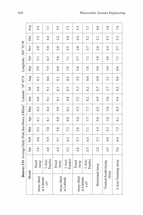
Photovoltaic Systems Engineering418
Avg 5.4
7.1
5.5
7.2
5.3
7.1
4.6
3.8
7.4
Dec 3.5
4.4
4.2
4.9
4.5
5.2
2.1
4.3
5.3
Nov 4.0
5.0
4.6
5.5
4.8
5.7
2.6
4.4
5.7
Oct
5.1
6.7
5.6
7.1
5.7
7.1
3.8
4.6
7.1
Sep
5.9
7.9
6.0
7.9
5.8
7.8
5.0
4.0
8.0
Aug 6.3
8.6
6.1
8.4
5.5
8.0
6.0
3.2
8.6
Jul
6.6
9.1
6.1
8.7
5.3
8.2
6.7
2.7
9.2
Jun
6.6
9.1
6.1
8.8
5.2
8.2
6.9
2.6
9.4
May
6.2
8.4
5.9
8.1
5.2
7.7
6.2
2.8
8.5
Apr
6.1
8.1
6.0
8.0
5.6
7.7
5.6
3.6
8.1
Mar
5.4
7.0
5.6
7.2
5.6
7.1
4.4
4.3
7.2
Feb
4.6
5.9
5.1
6.2
5.3
6.4
3.3
4.6
6.4
Jan
3.8
4.8
4.4
5.2
4.8
5.5
2.4
4.5
5.6
Fixe
dA
rray
1-A
xis
Tra
cker
Fixe
dA
rray
1-A
xis
Tra
cker
Fixe
dA
rray
1-A
xis
Tra
cker
Den
ver,
CO
Ave
rage
Dai
ly P
eak
Sun
Hou
rs, k
Wh/
m2
L
atitu
de:
39o 4
5’ N
L
ongi
tude
: 10
4o 5
2’ W
Mon
th
Arr
ay ti
lted
at L
atitu
de−1
5°
Arr
ay ti
lted
at L
atitu
de
Arr
ay ti
lted
at L
atitu
de+1
5 °
Hor
izon
tal A
rray
Ver
tical
Sou
th-f
acin
gA
rray
2-A
xis
Tra
ckin
g A
rray
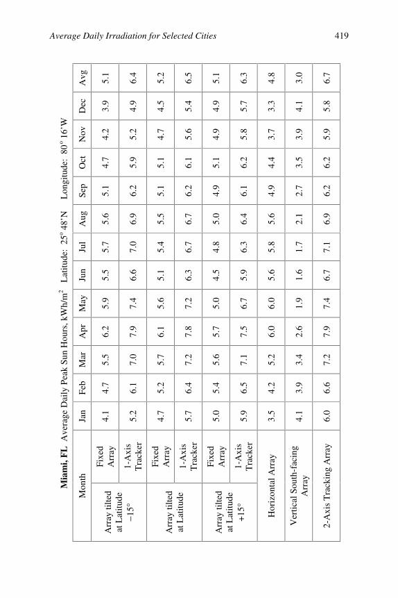
Average Daily Irradiation for Selected Cities 419
Avg 5.1
6.4
5.2
6.5
5.1
6.3
4.8
3.0
6.7
Dec 3.9
4.9
4.5
5.4
4.9
5.7
3.3
4.1
5.8
Nov 4.2
5.2
4.7
5.6
4.9
5.8
3.7
3.9
5.9
Oct
4.7
5.9
5.1
6.1
5.1
6.2
4.4
3.5
6.2
Sep
5.1
6.2
5.1
6.2
4.9
6.1
4.9
2.7
6.2
Aug 5.6
6.9
5.5
6.7
5.0
6.4
5.6
2.1
6.9
Jul
5.7
7.0
5.4
6.7
4.8
6.3
5.8
1.7
7.1
Jun
5.5
6.6
5.1
6.3
4.5
5.9
5.6
1.6
6.7
May
5.9
7.4
5.6
7.2
5.0
6.7
6.0
1.9
7.4
Apr
6.2
7.9
6.1
7.8
5.7
7.5
6.0
2.6
7.9
Mar
5.5
7.0
5.7
7.2
5.6
7.1
5.2
3.4
7.2
Feb
4.7
6.1
5.2
6.4
5.4
6.5
4.2
3.9
6.6
Jan
4.1
5.2
4.7
5.7
5.0
5.9
3.5
4.1
6.0
Fixe
dA
rray
1-A
xis
Tra
cker
Fixe
dA
rray
1-A
xis
Tra
cker
Fixe
dA
rray
1-A
xis
Tra
cker
Mia
mi,
FL
Ave
rage
Dai
ly P
eak
Sun
Hou
rs, k
Wh/
m2
L
atitu
de:
25o 4
8’ N
L
ongi
tude
: 80
o 16’
W
Mon
th
Arr
ay ti
lted
at L
atitu
de−1
5°
Arr
ay ti
lted
at L
atitu
de
Arr
ay ti
lted
at L
atitu
de+1
5 °
Hor
izon
tal A
rray
Ver
tical
Sou
th-f
acin
gA
rray
2-A
xis
Tra
ckin
g A
rray
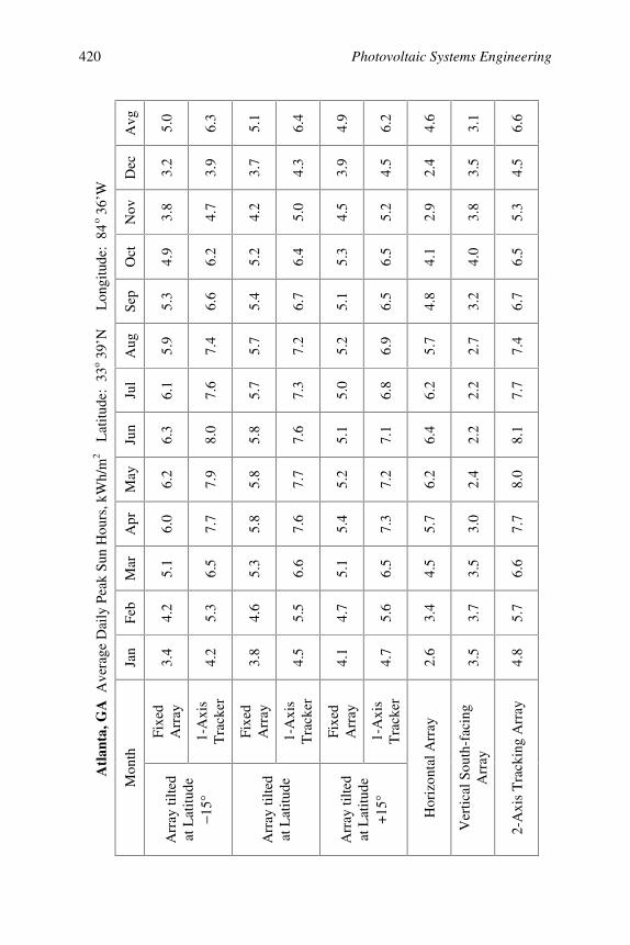
Photovoltaic Systems Engineering420
Avg 5.0
6.3
5.1
6.4
4.9
6.2
4.6
3.1
6.6
Dec 3.2
3.9
3.7
4.3
3.9
4.5
2.4
3.5
4.5
Nov 3.8
4.7
4.2
5.0
4.5
5.2
2.9
3.8
5.3
Oct
4.9
6.2
5.2
6.4
5.3
6.5
4.1
4.0
6.5
Sep
5.3
6.6
5.4
6.7
5.1
6.5
4.8
3.2
6.7
Aug 5.9
7.4
5.7
7.2
5.2
6.9
5.7
2.7
7.4
Jul
6.1
7.6
5.7
7.3
5.0
6.8
6.2
2.2
7.7
Jun
6.3
8.0
5.8
7.6
5.1
7.1
6.4
2.2
8.1
May
6.2
7.9
5.8
7.7
5.2
7.2
6.2
2.4
8.0
Apr
6.0
7.7
5.8
7.6
5.4
7.3
5.7
3.0
7.7
Mar
5.1
6.5
5.3
6.6
5.1
6.5
4.5
3.5
6.6
Feb
4.2
5.3
4.6
5.5
4.7
5.6
3.4
3.7
5.7
Jan
3.4
4.2
3.8
4.5
4.1
4.7
2.6
3.5
4.8
Fixe
dA
rray
1-A
xis
Tra
cker
Fixe
dA
rray
1-A
xis
Tra
cker
Fixe
dA
rray
1-A
xis
Tra
cker
Atl
anta
, GA
Ave
rage
Dai
ly P
eak
Sun
Hou
rs, k
Wh/
m2
L
atitu
de:
33o 3
9’ N
L
ongi
tude
: 84
o 36’
W
Mon
th
Arr
ay ti
lted
at L
atitu
de−1
5°
Arr
ay ti
lted
at L
atitu
de
Arr
ay ti
lted
at L
atitu
de+1
5 °
Hor
izon
tal A
rray
Ver
tical
Sou
th-f
acin
gA
rray
2-A
xis
Tra
ckin
g A
rray

Average Daily Irradiation for Selected Cities 421
Avg 4.5
5.7
4.6
5.7
4.4
5.6
3.9
3.2
5.9
Dec 2.5
2.9
2.9
3.2
3.1
3.4
1.6
2.9
3.4
Nov 2.8
3.4
3.1
3.6
3.3
3.7
1.9
3.0
3.8
Oct
4.1
5.0
4.3
5.2
4.4
5.2
3.0
3.6
5.3
Sep
5.0
6.3
5.1
6.4
4.9
6.2
4.3
3.5
6.4
Aug 5.7
7.3
5.5
7.1
5.0
6.8
5.4
3.1
7.3
Jul
6.0
7.8
5.6
7.5
4.9
7.0
6.1
2.8
7.9
Jun
6.0
7.7
5.5
7.4
4.8
6.9
6.1
2.6
7.9
May
5.7
7.3
5.3
7.1
4.7
6.6
5.6
2.8
7.4
Apr
5.2
6.5
5.0
6.5
4.7
6.2
4.7
3.1
6.6
Mar
4.6
5.7
4.7
5.9
4.6
5.8
3.7
3.7
5.9
Feb
3.8
4.7
4.2
5.0
4.3
5.1
2.7
3.9
5.1
Jan
3.0
3.6
3.4
3.9
3.6
4.1
1.9
3.4
4.1
Fixe
dA
rray
1-A
xis
Tra
cker
Fixe
dA
rray
1-A
xis
Tra
cker
Fixe
dA
rray
1-A
xis
Tra
cker
Bos
ton,
MA
Ave
rage
Dai
ly P
eak
Sun
Hou
rs, k
Wh/
m2
L
atitu
de:
41o 4
0’ N
L
ongi
tude
: 71
o 10’
W
Mon
th
Arr
ay ti
lted
at L
atitu
de−1
5°
Arr
ay ti
lted
at L
atitu
de
Arr
ay ti
lted
at L
atitu
de+1
5 °
Hor
izon
tal A
rray
Ver
tical
Sou
th-f
acin
gA
rray
2-A
xis
Tra
ckin
g A
rray
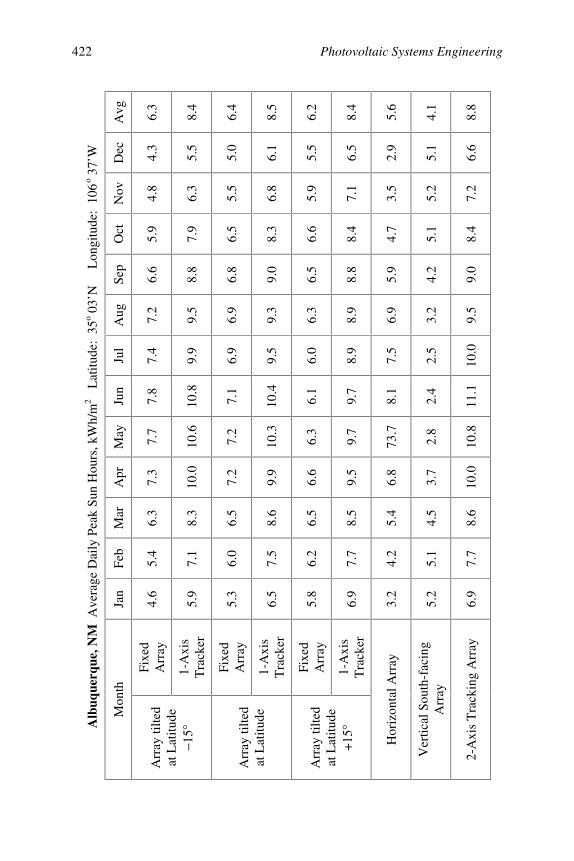
Photovoltaic Systems Engineering422
Avg 6.3
8.4
6.4
8.5
6.2
8.4
5.6
4.1
8.8
Dec 4.3
5.5
5.0
6.1
5.5
6.5
2.9
5.1
6.6
Nov 4.8
6.3
5.5
6.8
5.9
7.1
3.5
5.2
7.2
Oct
5.9
7.9
6.5
8.3
6.6
8.4
4.7
5.1
8.4
Sep
6.6
8.8
6.8
9.0
6.5
8.8
5.9
4.2
9.0
Aug 7.2
9.5
6.9
9.3
6.3
8.9
6.9
3.2
9.5
Jul
7.4
9.9
6.9
9.5
6.0
8.9
7.5
2.5
10.0
Jun
7.8
10.8
7.1
10.4
6.1
9.7
8.1
2.4
11.1
May
7.7
10.6
7.2
10.3
6.3
9.7
73.7
2.8
10.8
Apr
7.3
10.0
7.2
9.9
6.6
9.5
6.8
3.7
10.0
Mar
6.3
8.3
6.5
8.6
6.5
8.5
5.4
4.5
8.6
Feb
5.4
7.1
6.0
7.5
6.2
7.7
4.2
5.1
7.7
Jan
4.6
5.9
5.3
6.5
5.8
6.9
3.2
5.2
6.9
Fixe
dA
rray
1-A
xis
Tra
cker
Fixe
dA
rray
1-A
xis
Tra
cker
Fixe
dA
rray
1-A
xis
Tra
cker
Alb
uque
rque
, NM
Ave
rage
Dai
ly P
eak
Sun
Hou
rs, k
Wh/
m2
L
atitu
de:
35o 0
3’ N
L
ongi
tude
: 10
6o 3
7’ W
Mon
th
Arr
ay ti
lted
at L
atitu
de−1
5°
Arr
ay ti
lted
at L
atitu
de
Arr
ay ti
lted
at L
atitu
de+1
5 °
Hor
izon
tal A
rray
Ver
tical
Sou
th-f
acin
gA
rray
2-A
xis
Tra
ckin
g A
rray
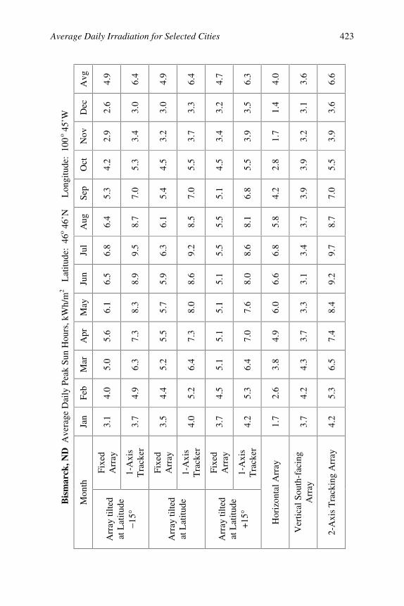
Average Daily Irradiation for Selected Cities 423
Avg 4.9
6.4
4.9
6.4
4.7
6.3
4.0
3.6
6.6
Dec 2.6
3.0
3.0
3.3
3.2
3.5
1.4
3.1
3.6
Nov 2.9
3.4
3.2
3.7
3.4
3.9
1.7
3.2
3.9
Oct
4.2
5.3
4.5
5.5
4.5
5.5
2.8
3.9
5.5
Sep
5.3
7.0
5.4
7.0
5.1
6.8
4.2
3.9
7.0
Aug 6.4
8.7
6.1
8.5
5.5
8.1
5.8
3.7
8.7
Jul
6.8
9.5
6.3
9.2
5.5
8.6
6.8
3.4
9.7
Jun
6.5
8.9
5.9
8.6
5.1
8.0
6.6
3.1
9.2
May
6.1
8.3
5.7
8.0
5.1
7.6
6.0
3.3
8.4
Apr
5.6
7.3
5.5
7.3
5.1
7.0
4.9
3.7
7.4
Mar
5.0
6.3
5.2
6.4
5.1
6.4
3.8
4.3
6.5
Feb
4.0
4.9
4.4
5.2
4.5
5.3
2.6
4.2
5.3
Jan
3.1
3.7
3.5
4.0
3.7
4.2
1.7
3.7
4.2
Fixe
dA
rray
1-A
xis
Tra
cker
Fixe
dA
rray
1-A
xis
Tra
cker
Fixe
dA
rray
1-A
xis
Tra
cker
Bis
mar
ck, N
D A
vera
ge D
aily
Pea
k Su
n H
ours
, kW
h/m
2
Lat
itude
: 46
o 46’
N
Lon
gitu
de:
100
o 45’
W
Mon
th
Arr
ay ti
lted
at L
atitu
de−1
5°
Arr
ay ti
lted
at L
atitu
de
Arr
ay ti
lted
at L
atitu
de+1
5 °
Hor
izon
tal A
rray
Ver
tical
Sou
th-f
acin
gA
rray
2-A
xis
Tra
ckin
g A
rray
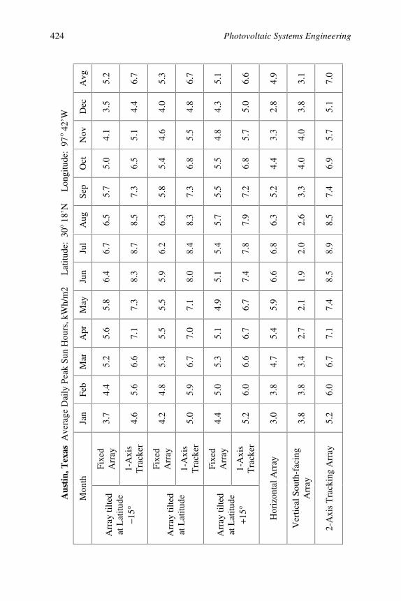
Photovoltaic Systems Engineering424
Avg 5.2
6.7
5.3
6.7
5.1
6.6
4.9
3.1
7.0
Dec 3.5
4.4
4.0
4.8
4.3
5.0
2.8
3.8
5.1
Nov 4.1
5.1
4.6
5.5
4.8
5.7
3.3
4.0
5.7
Oct
5.0
6.5
5.4
6.8
5.5
6.8
4.4
4.0
6.9
Sep
5.7
7.3
5.8
7.3
5.5
7.2
5.2
3.3
7.4
Aug 6.5
8.5
6.3
8.3
5.7
7.9
6.3
2.6
8.5
Jul
6.7
8.7
6.2
8.4
5.4
7.8
6.8
2.0
8.9
Jun
6.4
8.3
5.9
8.0
5.1
7.4
6.6
1.9
8.5
May
5.8
7.3
5.5
7.1
4.9
6.7
5.9
2.1
7.4
Apr
5.6
7.1
5.5
7.0
5.1
6.7
5.4
2.7
7.1
Mar
5.2
6.6
5.4
6.7
5.3
6.6
4.7
3.4
6.7
Feb
4.4
5.6
4.8
5.9
5.0
6.0
3.8
3.8
6.0
Jan
3.7
4.6
4.2
5.0
4.4
5.2
3.0
3.8
5.2
Fixe
dA
rray
1-A
xis
Tra
cker
Fixe
dA
rray
1-A
xis
Tra
cker
Fixe
dA
rray
1-A
xis
Tra
cker
Aus
tin,
Tex
as A
vera
ge D
aily
Pea
k Su
n H
ours
, kW
h/m
2
Lat
itude
: 30
o 18’
N
Lon
gitu
de:
97o 4
2’ W
Mon
th
Arr
ay ti
lted
at L
atitu
de−1
5°
Arr
ay ti
lted
at L
atitu
de
Arr
ay ti
lted
at L
atitu
de+1
5 °
Hor
izon
tal A
rray
Ver
tical
Sou
th-f
acin
gA
rray
2-A
xis
Tra
ckin
g A
rray
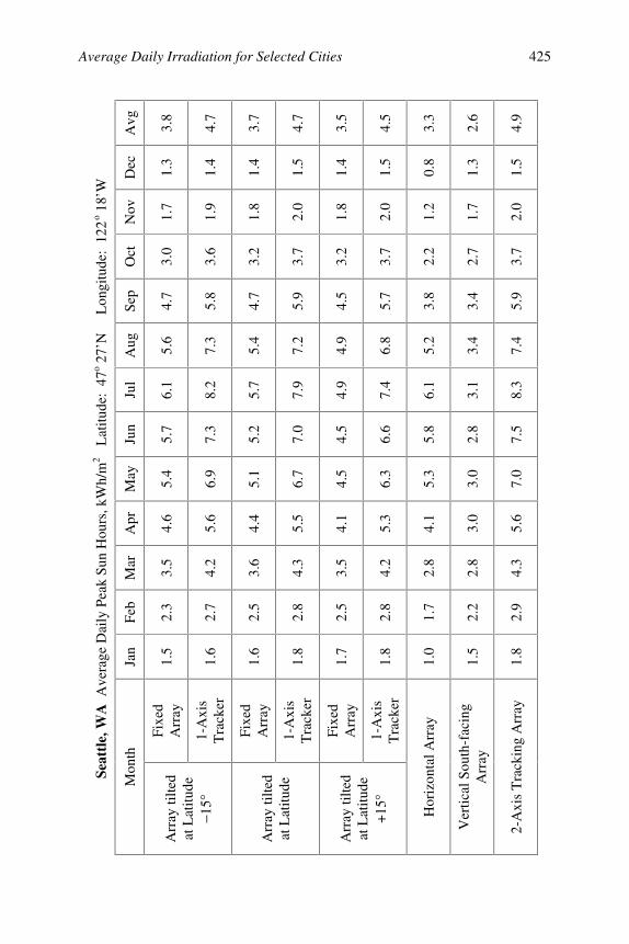
Average Daily Irradiation for Selected Cities 425
Avg 3.8
4.7
3.7
4.7
3.5
4.5
3.3
2.6
4.9
Dec 1.3
1.4
1.4
1.5
1.4
1.5
0.8
1.3
1.5
Nov 1.7
1.9
1.8
2.0
1.8
2.0
1.2
1.7
2.0
Oct
3.0
3.6
3.2
3.7
3.2
3.7
2.2
2.7
3.7
Sep
4.7
5.8
4.7
5.9
4.5
5.7
3.8
3.4
5.9
Aug 5.6
7.3
5.4
7.2
4.9
6.8
5.2
3.4
7.4
Jul
6.1
8.2
5.7
7.9
4.9
7.4
6.1
3.1
8.3
Jun
5.7
7.3
5.2
7.0
4.5
6.6
5.8
2.8
7.5
May
5.4
6.9
5.1
6.7
4.5
6.3
5.3
3.0
7.0
Apr
4.6
5.6
4.4
5.5
4.1
5.3
4.1
3.0
5.6
Mar
3.5
4.2
3.6
4.3
3.5
4.2
2.8
2.8
4.3
Feb
2.3
2.7
2.5
2.8
2.5
2.8
1.7
2.2
2.9
Jan
1.5
1.6
1.6
1.8
1.7
1.8
1.0
1.5
1.8
Fixe
dA
rray
1-A
xis
Tra
cker
Fixe
dA
rray
1-A
xis
Tra
cker
Fixe
dA
rray
1-A
xis
Tra
cker
Seat
tle,
WA
Ave
rage
Dai
ly P
eak
Sun
Hou
rs, k
Wh/
m2
L
atitu
de:
47o 2
7’ N
L
ongi
tude
: 12
2o 1
8’ W
Mon
th
Arr
ay ti
lted
at L
atitu
de−1
5°
Arr
ay ti
lted
at L
atitu
de
Arr
ay ti
lted
at L
atitu
de+1
5 °
Hor
izon
tal A
rray
Ver
tical
Sou
th-f
acin
gA
rray
2-A
xis
Tra
ckin
g A
rray
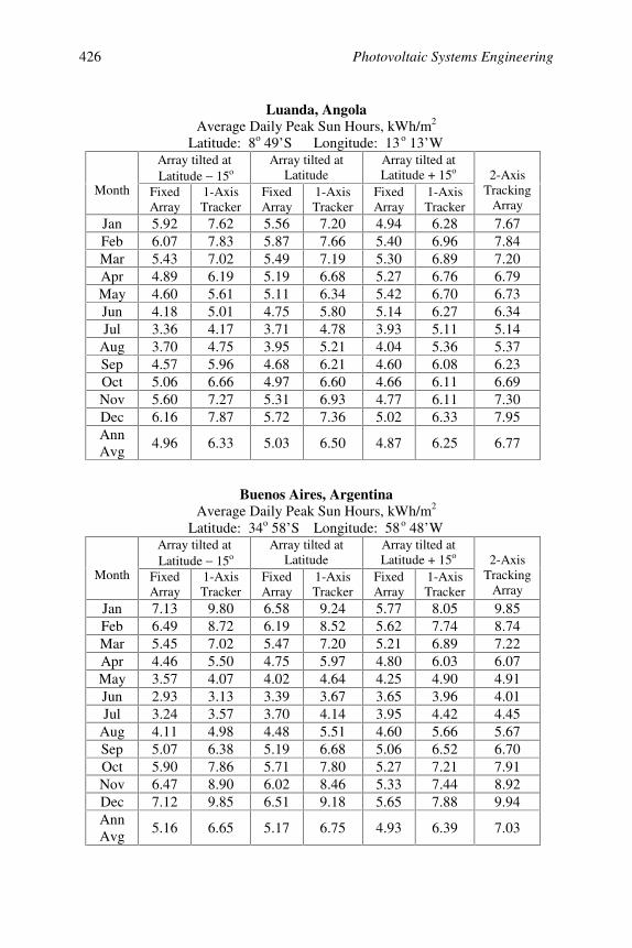
Photovoltaic Systems Engineering426
Luanda, AngolaAverage Daily Peak Sun Hours, kWh/m2
Latitude: 8o 49’ S Longitude: 13o 13’ WArray tilted at Latitude − 15o
Array tilted atLatitude
Array tilted atLatitude + 15o
Month FixedArray
1-AxisTracker
FixedArray
1-AxisTracker
FixedArray
1-AxisTracker
2-AxisTracking
Array
Jan 5.92 7.62 5.56 7.20 4.94 6.28 7.67Feb 6.07 7.83 5.87 7.66 5.40 6.96 7.84Mar 5.43 7.02 5.49 7.19 5.30 6.89 7.20Apr 4.89 6.19 5.19 6.68 5.27 6.76 6.79May 4.60 5.61 5.11 6.34 5.42 6.70 6.73Jun 4.18 5.01 4.75 5.80 5.14 6.27 6.34Jul 3.36 4.17 3.71 4.78 3.93 5.11 5.14
Aug 3.70 4.75 3.95 5.21 4.04 5.36 5.37Sep 4.57 5.96 4.68 6.21 4.60 6.08 6.23Oct 5.06 6.66 4.97 6.60 4.66 6.11 6.69Nov 5.60 7.27 5.31 6.93 4.77 6.11 7.30Dec 6.16 7.87 5.72 7.36 5.02 6.33 7.95AnnAvg
4.96 6.33 5.03 6.50 4.87 6.25 6.77
Buenos Aires, ArgentinaAverage Daily Peak Sun Hours, kWh/m2
Latitude: 34o 58’ S Longitude: 58o 48’ WArray tilted at Latitude − 15o
Array tilted atLatitude
Array tilted atLatitude + 15o
Month FixedArray
1-AxisTracker
FixedArray
1-AxisTracker
FixedArray
1-AxisTracker
2-AxisTracking
Array
Jan 7.13 9.80 6.58 9.24 5.77 8.05 9.85Feb 6.49 8.72 6.19 8.52 5.62 7.74 8.74Mar 5.45 7.02 5.47 7.20 5.21 6.89 7.22Apr 4.46 5.50 4.75 5.97 4.80 6.03 6.07May 3.57 4.07 4.02 4.64 4.25 4.90 4.91Jun 2.93 3.13 3.39 3.67 3.65 3.96 4.01Jul 3.24 3.57 3.70 4.14 3.95 4.42 4.45
Aug 4.11 4.98 4.48 5.51 4.60 5.66 5.67Sep 5.07 6.38 5.19 6.68 5.06 6.52 6.70Oct 5.90 7.86 5.71 7.80 5.27 7.21 7.91Nov 6.47 8.90 6.02 8.46 5.33 7.44 8.92Dec 7.12 9.85 6.51 9.18 5.65 7.88 9.94AnnAvg
5.16 6.65 5.17 6.75 4.93 6.39 7.03
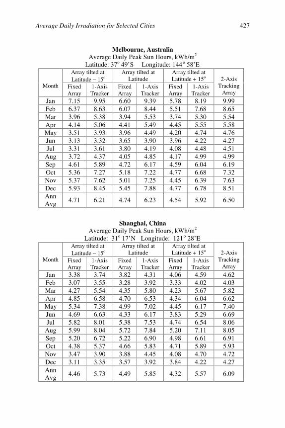
Average Daily Irradiation for Selected Cities 427
Melbourne, AustraliaAverage Daily Peak Sun Hours, kWh/m2
Latitude: 37o 49’ S Longitude: 144o 58’ EArray tilted at Latitude − 15o
Array tilted atLatitude
Array tilted atLatitude + 15o
Month FixedArray
1-AxisTracker
FixedArray
1-AxisTracker
FixedArray
1-AxisTracker
2-AxisTracking
Array
Jan 7.15 9.95 6.60 9.39 5.78 8.19 9.99Feb 6.37 8.63 6.07 8.44 5.51 7.68 8.65Mar 3.96 5.38 3.94 5.53 3.74 5.30 5.54Apr 4.14 5.06 4.41 5.49 4.45 5.55 5.58May 3.51 3.93 3.96 4.49 4.20 4.74 4.76Jun 3.13 3.32 3.65 3.90 3.96 4.22 4.27Jul 3.31 3.61 3.80 4.19 4.08 4.48 4.51
Aug 3.72 4.37 4.05 4.85 4.17 4.99 4.99Sep 4.61 5.89 4.72 6.17 4.59 6.04 6.19Oct 5.36 7.27 5.18 7.22 4.77 6.68 7.32Nov 5.37 7.62 5.01 7.25 4.45 6.39 7.63Dec 5.93 8.45 5.45 7.88 4.77 6.78 8.51AnnAvg
4.71 6.21 4.74 6.23 4.54 5.92 6.50
Shanghai, ChinaAverage Daily Peak Sun Hours, kWh/m2
Latitude: 31o 17’ N Longitude: 121o 28’ EArray tilted at Latitude − 15o
Array tilted atLatitude
Array tilted atLatitude + 15o
Month FixedArray
1-AxisTracker
FixedArray
1-AxisTracker
FixedArray
1-AxisTracker
2-AxisTracking
Array
Jan 3.38 3.74 3.82 4.31 4.06 4.59 4.62Feb 3.07 3.55 3.28 3.92 3.33 4.02 4.03Mar 4.27 5.54 4.35 5.80 4.23 5.67 5.82Apr 4.85 6.58 4.70 6.53 4.34 6.04 6.62May 5.34 7.38 4.99 7.02 4.45 6.17 7.40Jun 4.69 6.63 4.33 6.17 3.83 5.29 6.69Jul 5.82 8.01 5.38 7.53 4.74 6.54 8.06
Aug 5.99 8.04 5.72 7.84 5.20 7.11 8.05Sep 5.20 6.72 5.22 6.90 4.98 6.61 6.91Oct 4.38 5.37 4.66 5.83 4.71 5.89 5.93Nov 3.47 3.90 3.88 4.45 4.08 4.70 4.72Dec 3.11 3.35 3.57 3.92 3.84 4.22 4.27AnnAvg
4.46 5.73 4.49 5.85 4.32 5.57 6.09
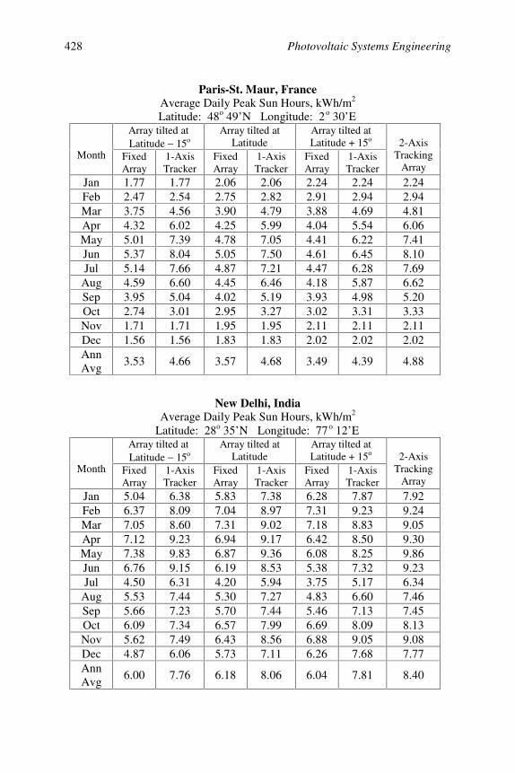
Photovoltaic Systems Engineering428
Paris-St. Maur, FranceAverage Daily Peak Sun Hours, kWh/m2
Latitude: 48o 49’ N Longitude: 2o 30’ EArray tilted at Latitude − 15o
Array tilted atLatitude
Array tilted atLatitude + 15o
Month FixedArray
1-AxisTracker
FixedArray
1-AxisTracker
FixedArray
1-AxisTracker
2-AxisTracking
Array
Jan 1.77 1.77 2.06 2.06 2.24 2.24 2.24Feb 2.47 2.54 2.75 2.82 2.91 2.94 2.94Mar 3.75 4.56 3.90 4.79 3.88 4.69 4.81Apr 4.32 6.02 4.25 5.99 4.04 5.54 6.06May 5.01 7.39 4.78 7.05 4.41 6.22 7.41Jun 5.37 8.04 5.05 7.50 4.61 6.45 8.10Jul 5.14 7.66 4.87 7.21 4.47 6.28 7.69
Aug 4.59 6.60 4.45 6.46 4.18 5.87 6.62Sep 3.95 5.04 4.02 5.19 3.93 4.98 5.20Oct 2.74 3.01 2.95 3.27 3.02 3.31 3.33Nov 1.71 1.71 1.95 1.95 2.11 2.11 2.11Dec 1.56 1.56 1.83 1.83 2.02 2.02 2.02AnnAvg
3.53 4.66 3.57 4.68 3.49 4.39 4.88
New Delhi, IndiaAverage Daily Peak Sun Hours, kWh/m2
Latitude: 28o 35’ N Longitude: 77o 12’ EArray tilted at Latitude − 15o
Array tilted atLatitude
Array tilted atLatitude + 15o
Month FixedArray
1-AxisTracker
FixedArray
1-AxisTracker
FixedArray
1-AxisTracker
2-AxisTracking
Array
Jan 5.04 6.38 5.83 7.38 6.28 7.87 7.92Feb 6.37 8.09 7.04 8.97 7.31 9.23 9.24Mar 7.05 8.60 7.31 9.02 7.18 8.83 9.05Apr 7.12 9.23 6.94 9.17 6.42 8.50 9.30May 7.38 9.83 6.87 9.36 6.08 8.25 9.86Jun 6.76 9.15 6.19 8.53 5.38 7.32 9.23Jul 4.50 6.31 4.20 5.94 3.75 5.17 6.34
Aug 5.53 7.44 5.30 7.27 4.83 6.60 7.46Sep 5.66 7.23 5.70 7.44 5.46 7.13 7.45Oct 6.09 7.34 6.57 7.99 6.69 8.09 8.13Nov 5.62 7.49 6.43 8.56 6.88 9.05 9.08Dec 4.87 6.06 5.73 7.11 6.26 7.68 7.77AnnAvg
6.00 7.76 6.18 8.06 6.04 7.81 8.40
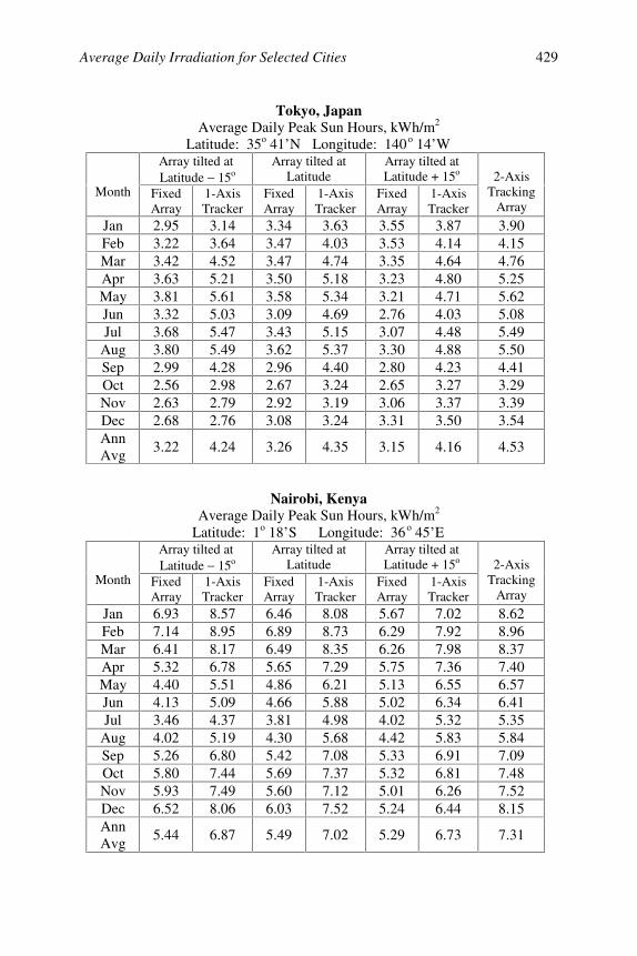
Average Daily Irradiation for Selected Cities 429
Tokyo, JapanAverage Daily Peak Sun Hours, kWh/m2
Latitude: 35o 41’ N Longitude: 140o 14’ WArray tilted at Latitude − 15o
Array tilted atLatitude
Array tilted atLatitude + 15o
Month FixedArray
1-AxisTracker
FixedArray
1-AxisTracker
FixedArray
1-AxisTracker
2-AxisTracking
Array
Jan 2.95 3.14 3.34 3.63 3.55 3.87 3.90Feb 3.22 3.64 3.47 4.03 3.53 4.14 4.15Mar 3.42 4.52 3.47 4.74 3.35 4.64 4.76Apr 3.63 5.21 3.50 5.18 3.23 4.80 5.25May 3.81 5.61 3.58 5.34 3.21 4.71 5.62Jun 3.32 5.03 3.09 4.69 2.76 4.03 5.08Jul 3.68 5.47 3.43 5.15 3.07 4.48 5.49
Aug 3.80 5.49 3.62 5.37 3.30 4.88 5.50Sep 2.99 4.28 2.96 4.40 2.80 4.23 4.41Oct 2.56 2.98 2.67 3.24 2.65 3.27 3.29Nov 2.63 2.79 2.92 3.19 3.06 3.37 3.39Dec 2.68 2.76 3.08 3.24 3.31 3.50 3.54AnnAvg
3.22 4.24 3.26 4.35 3.15 4.16 4.53
Nairobi, KenyaAverage Daily Peak Sun Hours, kWh/m2
Latitude: 1o 18’ S Longitude: 36o 45’ EArray tilted at Latitude − 15o
Array tilted atLatitude
Array tilted atLatitude + 15o
Month FixedArray
1-AxisTracker
FixedArray
1-AxisTracker
FixedArray
1-AxisTracker
2-AxisTracking
Array
Jan 6.93 8.57 6.46 8.08 5.67 7.02 8.62Feb 7.14 8.95 6.89 8.73 6.29 7.92 8.96Mar 6.41 8.17 6.49 8.35 6.26 7.98 8.37Apr 5.32 6.78 5.65 7.29 5.75 7.36 7.40May 4.40 5.51 4.86 6.21 5.13 6.55 6.57Jun 4.13 5.09 4.66 5.88 5.02 6.34 6.41Jul 3.46 4.37 3.81 4.98 4.02 5.32 5.35
Aug 4.02 5.19 4.30 5.68 4.42 5.83 5.84Sep 5.26 6.80 5.42 7.08 5.33 6.91 7.09Oct 5.80 7.44 5.69 7.37 5.32 6.81 7.48Nov 5.93 7.49 5.60 7.12 5.01 6.26 7.52Dec 6.52 8.06 6.03 7.52 5.24 6.44 8.15AnnAvg
5.44 6.87 5.49 7.02 5.29 6.73 7.31
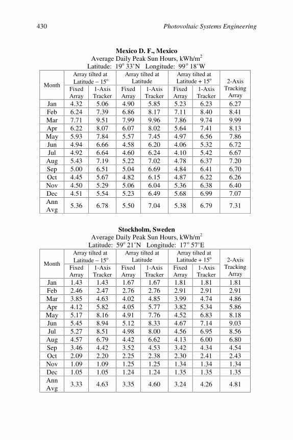
Photovoltaic Systems Engineering430
Mexico D. F., MexicoAverage Daily Peak Sun Hours, kWh/m2
Latitude: 19o 33’ N Longitude: 99o 18’ WArray tilted at Latitude − 15o
Array tilted atLatitude
Array tilted atLatitude + 15o
MonthFixedArray
1-AxisTracker
FixedArray
1-AxisTracker
FixedArray
1-AxisTracker
2-AxisTracking
Array
Jan 4.32 5.06 4.90 5.85 5.23 6.23 6.27Feb 6.24 7.39 6.86 8.17 7.11 8.40 8.41Mar 7.71 9.51 7.99 9.96 7.86 9.74 9.99Apr 6.22 8.07 6.07 8.02 5.64 7.41 8.13May 5.93 7.84 5.57 7.45 4.97 6.56 7.86Jun 4.94 6.66 4.58 6.20 4.06 5.32 6.72Jul 4.92 6.64 4.60 6.24 4.10 5.42 6.67
Aug 5.43 7.19 5.22 7.02 4.78 6.37 7.20Sep 5.00 6.51 5.04 6.69 4.84 6.41 6.70Oct 4.45 5.67 4.82 6.15 4.87 6.22 6.26Nov 4.50 5.29 5.06 6.04 5.36 6.38 6.40Dec 4.51 5.54 5.23 6.49 5.68 6.99 7.07AnnAvg
5.36 6.78 5.50 7.04 5.38 6.79 7.31
Stockholm, SwedenAverage Daily Peak Sun Hours, kWh/m2
Latitude: 59o 21’ N Longitude: 17o 57’ EArray tilted at Latitude − 15o
Array tilted atLatitude
Array tilted atLatitude + 15o
MonthFixedArray
1-AxisTracker
FixedArray
1-AxisTracker
FixedArray
1-AxisTracker
2-AxisTracking
Array
Jan 1.43 1.43 1.67 1.67 1.81 1.81 1.81Feb 2.46 2.47 2.76 2.76 2.91 2.91 2.91Mar 3.85 4.63 4.02 4.85 3.99 4.74 4.86Apr 4.12 5.82 4.05 5.77 3.82 5.34 5.86May 5.17 8.16 4.91 7.76 4.52 6.83 8.18Jun 5.45 8.94 5.12 8.33 4.67 7.14 9.03Jul 5.27 8.51 4.98 8.00 4.56 6.95 8.56
Aug 4.57 6.79 4.42 6.62 4.13 6.00 6.80Sep 3.46 4.42 3.52 4.53 3.42 4.34 4.54Oct 2.09 2.20 2.25 2.38 2.30 2.41 2.43Nov 1.09 1.09 1.25 1.25 1.34 1.34 1.34Dec 1.05 1.05 1.24 1.24 1.35 1.35 1.35AnnAvg
3.33 4.63 3.35 4.60 3.24 4.26 4.81

431
Appendix BA PARTIAL LISTING OF PV-RELATED WEB SITES
The following web sites represent a small sample of the hundreds of websites that list information on solar and renewable energy. The skilled web surferwill be able to find many more useful sites in a relatively short time. Listing of aweb site in this appendix does not constitute any endorsement by the authors orpublisher. Also, since web sites change continually, not all sites listed may existat the time of reading of this appendix.
Irradiance Data http://rredc.nrel.gov/solar/pubs/http://rredc.nrel.gov/solar/old_data/nsrdb/redbook/sum2/http://wrdc-mgo.nrel.gov/http://solstice.crest.org/renewables/solrad/
PV System http://www.shellsolar.com (module manufacturer)Components http://www.asepv.com (module manufacturer)Manufacturers http://www.kyocera.com (module manufacturer)and http://www.astropower.com (module manufacturer)Distributors http://www.sharpusa.com (module manufacturer)
http://www.evergreensolar.com (module manufacturer)http://www.bpsolar.com (module manufacturer)http://sma-america.com (inverters, etc.)http://www.xantrex.com (inverters, etc.)http://www.omnion.com (inverters, etc.)http://www.realgoods.com (retail distributor)http://www.SouthwestPV.com (retail distributor)http://www.windsun.com (retail distributor)http://www.solardirect.com (retail distributor)http://www.alt-energy.com (retail distributor)http://www.eco-web.com (retail distributor)http://www.poweriseverything.com (retail distributor)http://www.altenergystore.com (retail distributor)http://desotoenergy.com (retail distributor)http://www.cetsolar.com (retail distributor)http://www.mayberrys.com (generator distributor)http://www.batteries4everything.com (batteries)http://www.unirac.com (array mounts)http://www.zomeworks.com (array mounts)
Organizations, http://www.austinenergy.com (utility)Energy Data and http://www.smud.org (utilityUtility PV http://www.bpu.state.nj.us (state regulator)Projects http://www.eia.doe.gov/emeu/aer (energy information)
http://www.sandia.gov (research lab)http://www.dsireusa.org (state programs)

Photovoltaic Systems Engineering432
Environmental http://www.epa.gov/air/data/index.htmlSites http://www.wri.org/wr-96-97/ac_txt6.html
http://www.worldbank.orghttp://www.clean-power.comhttp://www.epa.gov/airmarkt/trading/buying.html
Financial ftp://ftp.bls.gov/pub/special.requests/cpi/cpiai.txtInformation http://djindexes.comSites ftp://ftp.ny.frb.org/prime/Prime.txt
In addition to the sites listed, the following site, maintained by the FloridaSolar Energy Center, contains an extensive list of links to a wide range ofenergy-related activity. General categories of the links available include:
Codes, Standards and Accreditation - Organizations and AssociationsColleges and UniversitiesElectrical, Construction and Labor - Unions, Organizations and AssociationsElectric Utilities, Organizations and Research CentersElectric Vehicles, Wind and Hydroelectric Energy SystemsElectrical, Electronic, Mechanical and Industrial EquipmentEnergy Efficiency and Renewable Energy-Related Directories and Link ListsEnergy-Efficient Lighting, Appliances, Equipment and Building SuppliesHoff’s Clean Power EstimatorInternational Governments and OrganizationsNational Laboratories and Research InstitutesPhotovoltaic Systems, Components and EngineeringRenewable Energy Education and TrainingRenewable Energy-Related Non-Governmental Organizations, Associations and
InformationRenewable Energy-Related Government Agencies, Departments and
LaboratoriesSpace, Meteorological and Ocean InformationSoftware and ComputerScience, Technology and Consumer InformationSolar Thermal Equipment - Domestic Water and Pool Heating and DesalinationSolar Radiation Data and InstrumentsState of Florida - Government, Departments and OrganizationsU.S. Federal - Government, Departments and OrganizationsWater World
For information on any of these areas, go to
http://www.fsec.ucf.edu
433
Appendix CDESIGN REVIEW CHECKLIST
The purpose of this textbook has been to prepare the engineer for the designof photovoltaic systems. The purpose of this Appendix is to provide a checklistagainst which the system designer can verify that sufficient information hasbeen provided in the design to meet the needs of whoever is given the tasks ofdesign review, installation, inspection, operation and maintenance of the de-signed system. To this end, the Florida Solar Energy Center has developed aDesign Review Checklist and Reporting Form. Following is a list of the itemson the Checklist that should be addressed in any grid-connected system design.The complete form, with space for comments on compliance, is available on theFSEC website (www.fsec.ucf.edu).
If design projects are assigned for a course that uses this book, it is recom-mended that the designs contain the information listed in this appendix.
I. System Documentation
A complete system documentation package is a fundamental requirement forsystem approvals. As a minimum, the system documentation package shouldinclude the following items. This information should be delivered to the end-user upon completion of the installation.
1. System description and specifications.2. Lists and specifications for parts and equipment supplied and not sup-
plied with any package system.3. Electrical diagrams and schematics with all items in the following sec-
tion on electrical design.4. Mechanical drawings with all items in the following section on me-
chanical design.5. System installation and checkout procedures.6. Safety instructions and hazard warnings for installation, operation and
maintenance of the system.7. Owner’s operating instructions.8. Owner’s manuals, specification sheets and warranty information for in-
dividual major system components.
II. Electrical Design
The electrical system design must be consistent with the latest version of theNational Electrical Code and should, as a minimum, provide a system schematicdiagram that includes the following information. Local code enforcement offi-cials may require an engineering seal on the electrical prints.
1. Description of methods and materials for wiring of the PV modules,panels and arrays.
Photovoltaic Systems Engineering434
2. Specification of appropriate types, sizes, ratings and locations for allsystem conductors.
3. Specification of the appropriate types, sizes, ratings and locations forconduit, wireways and junction boxes to be used in the installation.
4. Specification of appropriate ratings and locations for required overcur-rent devices.
5. Specification of appropriate ratings and locations for required discon-nect devices.
6. Specification of requirements, conductors and locations for equipmentand system grounding.
7. Specification of and diagrams for the methods and equipment requiredto interface the PV system output with the electric utility grid.
III. Mechanical Design
Methods for the safe, secure and durable attachment of PV arrays to rooftopsor other support structures is an essential part of a complete design package.Local code enforcement officials may require a mechanical engineer to seal themechanical prints. The prints, as a minimum, should include the following in-formation on mechanical components of the system.
1. For rooftop mounting, guidelines for locating and orienting the array onthe rooftop.
2. Guidelines for the mechanical assembly of modules and panels.3. Specification of hardware for proper mechanical assembly of modules
and panels.4. Diagrams and procedures for making structural attachments to roofs.5. Specification of hardware for making structural attachments to roofs.6. Description of appropriate methods of weathersealing rooftop attach-
ment points.7. Independent test results or engineering approval that the array mount-
ing system design is capable of withstanding maximum forces antici-pated for the location of the system (e.g., wind, snow or earthquakeloads.)
IV. PV Modules and Array
Information should be provided that verifies that the PV modules proposedfor the system have been properly listed, along with performance data for themodules. As a minimum, the following information should be supplied.
1. Module performance test results from an independent test laboratory.2. Indication of compliance with IEEE 1262, IEC 61215 or 61646 module
qualification tests.3. Indication of compliance with UL 1703 or equivalent product safety
testing.

Design Review Checklist 435
V. Power Conditioning Equipment and Batteries
As a minimum, the following information should be provided for inverters,chargers, charge controllers, batteries and other power processing equipment.
1. Compliance of inverter with UL 1741 and IEEE 929-2000 if used in agrid connected system.
2. Evidence that voltage operating windows under temperature extremesare acceptable.
3. Verification that charge controller set points are appropriate for thesystem batteries that are selected.
4. Locations for power conditioning equipment and batteries that are con-sistent with appropriate codes.