Embed Size (px)
Citation preview
Master Level Thesis
European Solar Engineering School
No.194, June 2015
Photovoltaic System Design for a Contaminated Area in Falun –
Comparison of South and East-West Layout
Master thesis 15 hp, 2015 Solar Energy Engineering
Author: Anton Fedorov
Supervisor: Frank Fiedler
Examiner: Ewa Wäckelgård
Course Code: MÖ3031
Examination date: 2015-06-11
Dalarna University
Energy and Environmental
Technology

ii
iii
Abstract In this thesis the solar part of a large grid-connected photovoltaic system design has been done. The main purpose was to size and optimize the system and to present figures helping to evaluate the prospective project rationality, which can potentially be constructed on a contaminated area in Falun. The methodology consisted in PV market study and component selection, site analysis and defining suitable area for solar installation; and system configuration optimization based on PVsyst simulations and Levelized Cost of Energy calculations. The procedure was mainly divided on two parts, preliminary and detailed sizing. In the first part the objective was complex, which included the investigation of the most profitable component combination and system optimization due to tilt and row distance. It was done by simulating systems with different components and orientations, which were sized for the same 100kW inverter in order to make a fair comparison. For each simulated result a simplified LCOE calculation procedure was applied. The main results of this part show that with the price of 0.43 €/Wp thin-film modules were the most cost effective solution for the case with a great advantage over crystalline type in terms of financial attractiveness. From the results of the preliminary study it was possible to select the optimal system configuration, which was used in the detailed sizing as a starting point. In this part the PVsyst simulations were run, which included full scale system design considering near shadings created by factory buildings. Additionally, more complex procedure of LCOE calculation has been used here considered insurances, maintenance, time value of money and possible cost reduction due to the system size. Two system options were proposed in final results; both cover the same area of 66000 m2. The first one represents an ordinary South faced design with 1.1 MW nominal power, which was optimized for the highest performance. According to PVsyst simulations, this system should produce 1108 MWh/year with the initial investment of
835,000 € and 0.056 €/kWh LCOE. The second option has an alternative East-West orientation, which allows to cover 80% of occupied ground and consequently have 6.6 MW PV nominal power. The system produces 5388 MWh/year costs about 4500,000 € and delivers electricity with the same price of 0.056 €/kWh. Even though the EW solution has 20% lower specific energy production, it benefits mainly from lower relative costs for inverters, mounting and annual maintenance expenses. After analyzing the performance results, among the two alternatives none of the systems showed a clear superiority so there was no optimal system proposed. Both, South and East-West solutions have own advantages and disadvantages in terms of energy production profile, configuration, installation and maintenance. Furthermore, the uncertainty due to cost figures assumptions restricted the results veracity.

iv
Acknowledgment First of all, I would like to dedicate this thesis to my friends and other people who are involved in the Ukrainian war, risking their lives to keep it in piece. I would like to express a special gratitude to my program coordinator and academic supervisor Frank Fiedler and the director of international recruitment of Dalarna University Michael Oppenheimer. My education would not have been possible without the help and support of these persons. I would like to sincerely thank Falu Energi & Vatten for giving me the opportunity and honor to write this thesis. I would also like to thank the company Solibro for their support and will to share information. In a personal note I would like to thank my family, friends and my dear wife for their support and belief in me throughout this time. Special thanks to Britt-Marie Wiktorsson and Alexandros Angelopoulos for medical care provision when I was unhealthy.
v
Contents i
Abstract ........................................................................................................................................... iii
Acknowledgment ........................................................................................................................... iv
Contents ........................................................................................................................................... v
List of figures ................................................................................................................................. vi
List of tables .................................................................................................................................. vii
Nomenclature ............................................................................................................................... viii
1 Introduction ................................................................................................................................. 1 1.1 Aims ........................................................................................................................................... 2 1.2 Method ....................................................................................................................................... 3 1.3 Previous work ........................................................................................................................... 3
2 Background information ............................................................................................................ 9 2.1 Boundary conditions ................................................................................................................ 9
2.1.1. Location, orientation and relief ................................................................................. 9 2.1.2. Metrological data ....................................................................................................... 10 2.1.3. Shading ....................................................................................................................... 11 2.1.4. Grid connection ........................................................................................................ 12
2.2 Site analysis .............................................................................................................................. 12
3 Components selection and system sizing ............................................................................... 13 3.1 Component selection ............................................................................................................. 13
3.1.1. Modules ...................................................................................................................... 14 3.1.2. Inverters ...................................................................................................................... 15 3.1.3. Mounting and other electrical components .......................................................... 17
3.2 Preliminary sizing ................................................................................................................... 17 3.2.1. String sizing and numbering .................................................................................... 18 3.2.2. Row spacing factor and tilt ...................................................................................... 20
3.3 Detailed sizing ......................................................................................................................... 23 3.3.1. South oriented system .............................................................................................. 24 3.3.2. Module arrangement factor for South orientation ............................................... 25 3.3.3. East-West oriented system ...................................................................................... 27
3.4 Economical evaluation procedure ....................................................................................... 28 3.4.1. System scale factor .................................................................................................... 30
3.5 Limitations and constraints ................................................................................................... 30 3.5.1. Site topography .......................................................................................................... 30 3.5.2. Geographical position and metrologilal data ........................................................ 30 3.5.3. Shadings ...................................................................................................................... 31 3.5.4. Irradiation calculation method ................................................................................ 31 3.5.5. Electrical and mechanical layout ............................................................................. 32 3.5.6. Economical evaluation procedure .......................................................................... 32
4 Results and analysis ................................................................................................................... 32 4.1 Preliminary sizing results ....................................................................................................... 33
4.1.1. Optimization due to inverter oversizing ................................................................ 33 4.1.2. Optimization due to module type, tilt and between row distance ..................... 33 4.1.3. Possible system size analysis .................................................................................... 35
4.2 Detailed design results ........................................................................................................... 37 4.2.1. System performance analysis ................................................................................... 37 4.2.2. Economical evaluation ............................................................................................. 39
vi
5 Discussion .................................................................................................................................. 42
6 Conclusion .................................................................................................................................. 43
Appendix A: Component Specification Sheets ........................................................................ 47
Appendix B: Results of PVsyst simulations and LCOEA calculations for preliminary designed systems with 100kW inverter. ..................................................................................... 56
Appendix C: Losses diagram comparison for systems with different modules, the same 100kW inverter, 10m between row distance and the optimal tilt. ........................................ 57
Appendix D: PVsyst report for detailed sizing, South orientated system ............................ 58
Appendix E: PVsyst report for detailed sizing, East orientated system ............................... 63
Appendix F: PVsyst report for detailed sizing, West orientated system .............................. 68
List of figures Fig. 1.1 Aerial view of Falun and the studied area. .................................................................... 2 Fig. 1.2 Side view of tilted array showing solar altitude angle. ................................................. 4 Fig. 1.3 Top view of tilted array showing solar azimuth correction. ....................................... 5 Fig. 1.4 The distance between rows to avoid shading due to the PV module in front. ....... 5 Fig. 1.5 Module-to-cell width is measured across the PV modules’ row................................ 6 Fig. 2.1 Aerial view of the studied site. ........................................................................................ 9 Fig. 2.2 Topographic map of the studied site. .......................................................................... 10 Fig. 2.3 Horizon shading profile. ................................................................................................ 11 Fig. 2.4 Aerial view of the site from the North.. ...................................................................... 12 Fig. 2.5 Three dimensional site view with indication of available area for PV installation.. .................................................................................................................................... 13 Fig. 3.1 Graphical dependence of pricing per continuous inverter Watt in Euro per W/p on inverter nominal power. ............................................................................................... 16 Fig. 3.2 Efficiency curves of 100kW ABB inverter chosen for preliminary design.. .......... 19 Fig. 3.3 Graphical dependence of global irradiation on collector plane and related losses on plane tilt.. ....................................................................................................................... 20 Fig. 3.4 Graphical dependence of annual system energy production on plane tilt. ........... 21 Fig. 3.5 Shed mutual shading for 45° tilted plane for Borlänge. ............................................ 22 Fig. 3.6 Graphical dependence of global irradiation on collector plane on plane tilt. ........ 22 Fig. 3.7 Distances between rows for East-West orientation. ................................................. 23 Fig. 3.8 Efficiency curves of 400kW ABB PVI-400-TL inverter .......................................... 24 Fig. 3.9 Perspective view of simulated array and factory buildings for South oriented system. ............................................................................................................................................ 25 Fig. 3.10 Side view of tilted array showing possible row distance correction and related parameters according to height difference. ............................................................................... 26 Fig. 3.11 Graphical dependence of module row distance according to height difference variation.. ........................................................................................................................................ 27 Fig. 3.12 Perspective view of simulated array and factory buildings for East oriented system. ............................................................................................................................................ 28 Fig. 4.1 Graphical dependence of Levelized Cost of Energy on annual basis and system losses due to inverter undersizing on module to inverter nominal power ratio ..... 33 Fig. 4.2 Graphical dependence of Levelized Cost of Energy on annual basis over between row distance. .................................................................................................................. 35 Fig. 4.3 Graphical dependence of Levelized Cost of Energy on annual basis and possible system nominal power on between row distance for thin-film modules with South orientation. ......................................................................................................................... 36
vii
Fig. 4.4 Graphical dependence of Levelized Cost of Energy on annual basis on possible system nominal power. ................................................................................................. 36 Fig. 4.5 Performance Ratio comparison for South and East orientation. ............................ 38 Fig. 4.6 Monthly hourly average energy production for June for South, East, West and East-West oriented system. ......................................................................................................... 38 Fig. 4.7 Annual monthly average energy production for South, East, West and East-West oriented system. .................................................................................................................. 39 Fig. 4.8 Costs breakdown for South oriented 1.1MW system (to the left) and for East-West 6.65MW system ................................................................................................................... 40
List of tables Table 1.1 Equation parameters for different shares of the diffuse light ................................ 6 Table 2.1 Monthly Meteo values for Borlänge, Sweden. ........................................................ 11 Table 2.2 Measured horizon shading data. ................................................................................ 11 Table 3.1 Module characteristics and costs for three options being analyzed. .................... 15 Table 3.2 Prices of inverters considered in the design ............................................................ 17 Table 3.3 Cost figures for PV mounting system in Euro/Wp, according to PV nominal power. ............................................................................................................................................. 17 Table 3.4 Cost figures for PV Balance Of System components as a share of total equipment costs ............................................................................................................................ 17 Table 3.5 Maximum possible module output voltage for the location and maximum number of module in strings considering 1000V as the highest allowable inverter input voltage. ........................................................................................................................................... 18 Table 3.6 Chosen string numbering parameters for preliminary design............................... 20 Table 3.7 Chosen array design parameters for South oriented system. ................................ 25 Table 3.8 Chosen array design parameters for East-West oriented system. ........................ 27 Table 3.9 Solar PV plant operation and maintenance cost estimates. .................................. 30 Table 4.1 Final PVsyst simulations results. ............................................................................... 37 Table 4.2 Final pricing of the proposed 1.1MW South oriented system, 6.65MW East-West oriented system and the same East-West system including possible cost reduction due to system scale. .................................................................................................... 40 Table 4.3 Final Lvelized Cost of Energy for the proposed 1.1MW South oriented system, 6.65MW East-West oriented system ............................................................................ 41
viii
Nomenclature A Energy loss parameter
AC Alternating current electricity
ACOLL Total collector gross area
AEP
Initial annual energy production
AGROUND Occupied ground area
AO
Annual operating and maintenance costs
BOS Balance of System
CIGS Copper Indium Gallium (di) Selenide
CO2 Carbon Dioxide
D (D’) Distance between rows, meter
DC Direct current electricity
DCOR Corrected between row distance, meter
EUR EURO currency
EW East-West oriented system
F Spacing factor
FOCCUP Ground area occupation ratio
H Height of array obstruction, meter
I Annual insurance
IC Initial project costs
IMPP Maximum power point current
KT Module temperature coefficient, %/°C
L Module length (width), meter
LCOE Levelized Cost of Energy
LCOEA
Levelized Cost of Energy on annual basis
MPP Maximum power point
MPPT Maximum power point tracking
n Project lifetime in years
O&M Operation and maintenance
PR Performance ratio
PV Photovoltaics
RAEL Relative annual energy loss
SDR System degradation rate
SEK Swedish Krona
SERC Solar Energy Research Center
Si-mono Monocrystalline silicon
Si-poly Polycrystalline silicon
STC Standard test conditions, irradiation 1000 W/m² and module temperature 25°C
TMOD Lowest possible temperature during day, °C
TO Total operating and maintenance costs over project lifetime
VMAX Maximum module output voltage, volts
VMPP Voltage at maximum power point, volts
Voc Open circuit voltage, volts
Wp Nominal power, Watt peak
α Solar altitude angle, °
β Array tilt, °
θ Solar zenith angle, °
ψ Solar azimuth angle, °
1
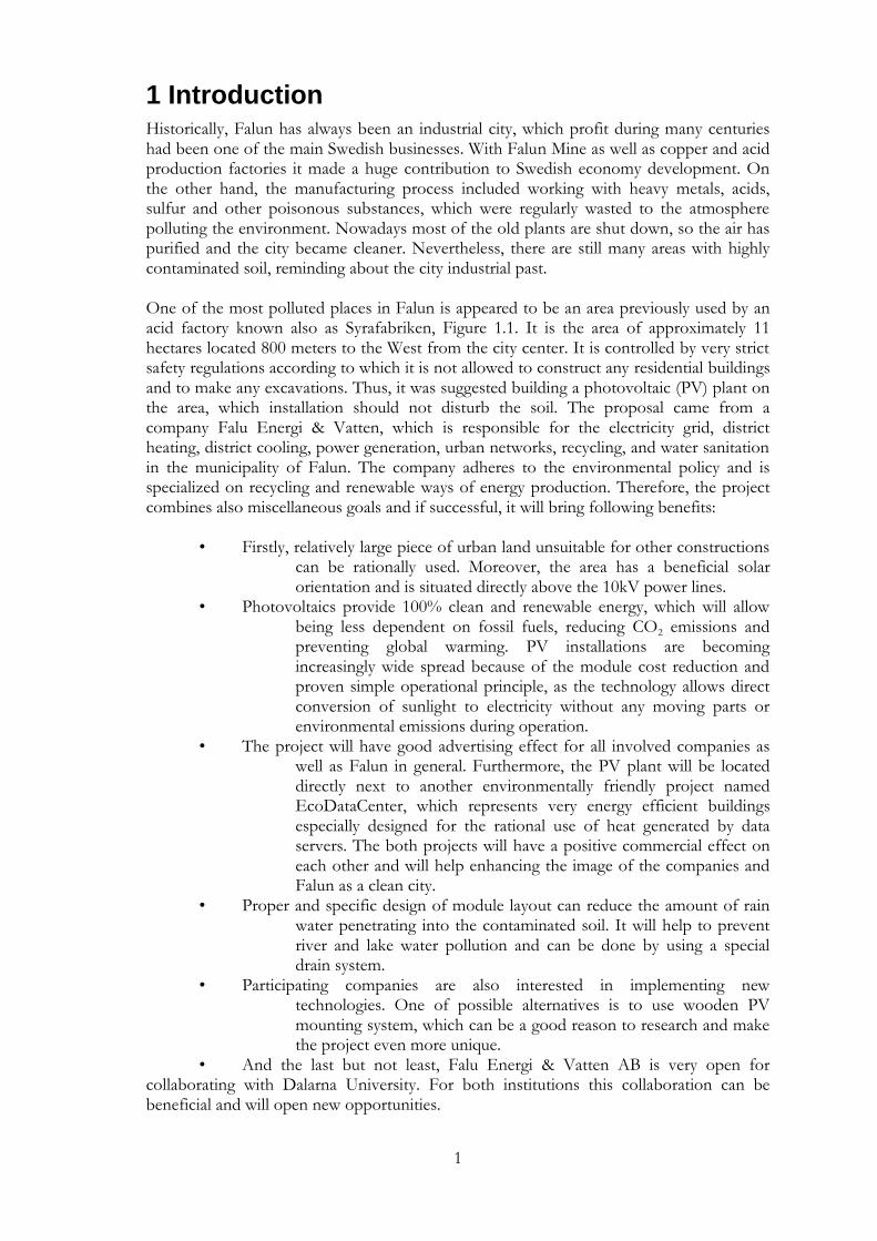
1 Introduction Historically, Falun has always been an industrial city, which profit during many centuries had been one of the main Swedish businesses. With Falun Mine as well as copper and acid production factories it made a huge contribution to Swedish economy development. On the other hand, the manufacturing process included working with heavy metals, acids, sulfur and other poisonous substances, which were regularly wasted to the atmosphere polluting the environment. Nowadays most of the old plants are shut down, so the air has purified and the city became cleaner. Nevertheless, there are still many areas with highly contaminated soil, reminding about the city industrial past. One of the most polluted places in Falun is appeared to be an area previously used by an acid factory known also as Syrafabriken, Figure 1.1. It is the area of approximately 11 hectares located 800 meters to the West from the city center. It is controlled by very strict safety regulations according to which it is not allowed to construct any residential buildings and to make any excavations. Thus, it was suggested building a photovoltaic (PV) plant on the area, which installation should not disturb the soil. The proposal came from a company Falu Energi & Vatten, which is responsible for the electricity grid, district heating, district cooling, power generation, urban networks, recycling, and water sanitation in the municipality of Falun. The company adheres to the environmental policy and is specialized on recycling and renewable ways of energy production. Therefore, the project combines also miscellaneous goals and if successful, it will bring following benefits:
• Firstly, relatively large piece of urban land unsuitable for other constructions can be rationally used. Moreover, the area has a beneficial solar orientation and is situated directly above the 10kV power lines.
• Photovoltaics provide 100% clean and renewable energy, which will allow being less dependent on fossil fuels, reducing CO2 emissions and preventing global warming. PV installations are becoming increasingly wide spread because of the module cost reduction and proven simple operational principle, as the technology allows direct conversion of sunlight to electricity without any moving parts or environmental emissions during operation.
• The project will have good advertising effect for all involved companies as well as Falun in general. Furthermore, the PV plant will be located directly next to another environmentally friendly project named EcoDataCenter, which represents very energy efficient buildings especially designed for the rational use of heat generated by data servers. The both projects will have a positive commercial effect on each other and will help enhancing the image of the companies and Falun as a clean city.
• Proper and specific design of module layout can reduce the amount of rain water penetrating into the contaminated soil. It will help to prevent river and lake water pollution and can be done by using a special drain system.
• Participating companies are also interested in implementing new technologies. One of possible alternatives is to use wooden PV mounting system, which can be a good reason to research and make the project even more unique.
• And the last but not least, Falu Energi & Vatten AB is very open for collaborating with Dalarna University. For both institutions this collaboration can be beneficial and will open new opportunities.
2
As it can be seen from above, the project is quite reasonable, has good perspectives and high chances to be implemented. Nevertheless, the crucial argument for the company is still the economical profitability, which can be represented as a Levelised Cost of Energy (LCOE) value. Therefore, a prestudy of a PV plant has already been done by the company Kraftpojkarna, specialized on solar tracking systems. However, being a specific product, solar trackers are usually more expensive solution, which might make the plant less financially attractive. So Falu Energi & Vatten, which is responsible for the project is interested in making a research and investigate more system options to find out the optimal design solution for the case from a financial perspective. These facts provide a suitable reason for this thesis and further research.
1.1 Aims
The main aim of the thesis is to design a PV plant to optimally cover the polluted area and to find the most financially attractive combination of used components and system layout. In addition, it is aimed to make an alternative system design, which should cover as much as possible of the site area in order to reduce rain water penetration into the contaminated soil. Then to analyze the results and make a performance and financial comparison between the two options. Despite a great will of the author, it was impossible to cover all details of the design in terms of the thesis due to time, information and experience limitations. Therefore, the work is mainly focused on the solar part of the design, whereas for other aspects simplified solutions with certain assumptions had to be chosen.
Fig. 1.1. Aerial view of Falun and the studied territory (Wikimapia, 2015). Fig. 1. 1 Aerial view of Falun and the studied territory (Wikimapia, 2015). Fig. 1.1 Aerial view of Falun and the studied area (Wikimapia, 2015).
3
1.2 Method
The thesis is mainly based on PVsyst simulations and economical evaluation procedure. Therefore, the work process was planned according to following steps:
Firstly, to study the previous design and related literature and analyze the results. To acquire the advanced knowledge of PVsyst software.
The next step was to define the boundary conditions for the case, which included horizon shading measurements and shading map creation. To determine possible assumptions and limitations.
To analyze the site topography for potential shadings and determine the suitable area for PV installation.
To study the European Photovoltaic market superficially and to find the potential component supplier companies. To contact the companies in order to find out the precise prices for system components. To select several suitable component alternatives based on quality, warranty and the most competitive costs.
After this a preliminary system design has been done. This step covered the design and simulations of systems with different modules and the same inverter, which helped to define the optimal components for the case.
To perform a number of simulations varying the module tilt and the distance between panel arrays for South orientation. To analyze the results and choose the optimal combination.
To simulate a separate system with alternative East-West (EW) module orientation in preliminary sizing and evaluate the rationality of this solution.
According to the results of preliminary design to define the possible system sizes for different configurations.
To create a 3D model of potential near shading objects in PVsyst.
To make two detailed system design simulations, the first with optimized South oriented system and the second with the EW orientation. For each system to make an economical evaluation according to Levelized Cost of Energy (LCOE).
To analyze the system performance for both cases on daily, monthly and yearly basis.
Finally, to discuss the results and make a conclusion.
1.3 Previous work
As mentioned before, a pre-study has already been done by Kraftpojkarna AB (Lindblad, 2014). It is a Swedish company, which specializes on solar tracking systems. This technology includes a special controlled mounting system which keeps modules always in optimal orientation to the sun during operation. The advantage of this design is that it allows absorbing maximum solar irradiation and increasing the amount of produced energy per module area as a result. However, the complexity of this alternative makes it more expensive and maintenance demanding. Three system alternatives are presented in the report. In the first one the array consists of 83 solar trackers with 36 solar panels or 72 square meters per each unit. It gives the PV area of 5976 m2 in total and the trackers are placed in the field so that the system has the highest possible efficiency. The PV output power is 950 kW and annual energy production constitutes 1430 MWh. Even though this solution has the highest LCOE, the company claims about its advantages. Firstly, trackers provide higher efficiency and work automatically even in winter by setting themselves so that the snow slides off. Secondly, it will help to reduce the sunlight reflection from modules that could disturb automobile
4
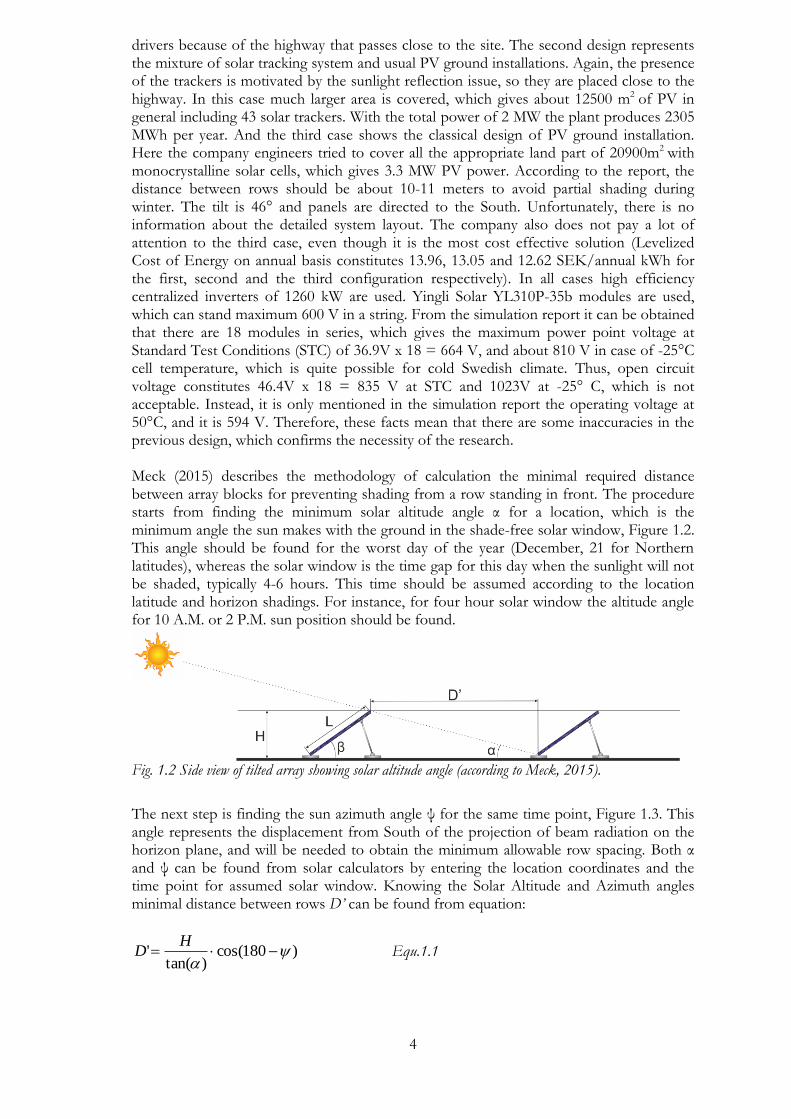
drivers because of the highway that passes close to the site. The second design represents the mixture of solar tracking system and usual PV ground installations. Again, the presence of the trackers is motivated by the sunlight reflection issue, so they are placed close to the highway. In this case much larger area is covered, which gives about 12500 m2 of PV in general including 43 solar trackers. With the total power of 2 MW the plant produces 2305 MWh per year. And the third case shows the classical design of PV ground installation. Here the company engineers tried to cover all the appropriate land part of 20900m2 with monocrystalline solar cells, which gives 3.3 MW PV power. According to the report, the distance between rows should be about 10-11 meters to avoid partial shading during winter. The tilt is 46° and panels are directed to the South. Unfortunately, there is no information about the detailed system layout. The company also does not pay a lot of attention to the third case, even though it is the most cost effective solution (Levelized Cost of Energy on annual basis constitutes 13.96, 13.05 and 12.62 SEK/annual kWh for the first, second and the third configuration respectively). In all cases high efficiency centralized inverters of 1260 kW are used. Yingli Solar YL310P-35b modules are used, which can stand maximum 600 V in a string. From the simulation report it can be obtained that there are 18 modules in series, which gives the maximum power point voltage at Standard Test Conditions (STC) of 36.9V x 18 = 664 V, and about 810 V in case of -25°C cell temperature, which is quite possible for cold Swedish climate. Thus, open circuit voltage constitutes 46.4V x 18 = 835 V at STC and 1023V at -25° C, which is not acceptable. Instead, it is only mentioned in the simulation report the operating voltage at 50°C, and it is 594 V. Therefore, these facts mean that there are some inaccuracies in the previous design, which confirms the necessity of the research. Meck (2015) describes the methodology of calculation the minimal required distance between array blocks for preventing shading from a row standing in front. The procedure starts from finding the minimum solar altitude angle α for a location, which is the minimum angle the sun makes with the ground in the shade-free solar window, Figure 1.2. This angle should be found for the worst day of the year (December, 21 for Northern latitudes), whereas the solar window is the time gap for this day when the sunlight will not be shaded, typically 4-6 hours. This time should be assumed according to the location latitude and horizon shadings. For instance, for four hour solar window the altitude angle for 10 A.M. or 2 P.M. sun position should be found.
Fig. 1.2 Side view of tilted array showing solar altitude angle (according to Meck, 2015).
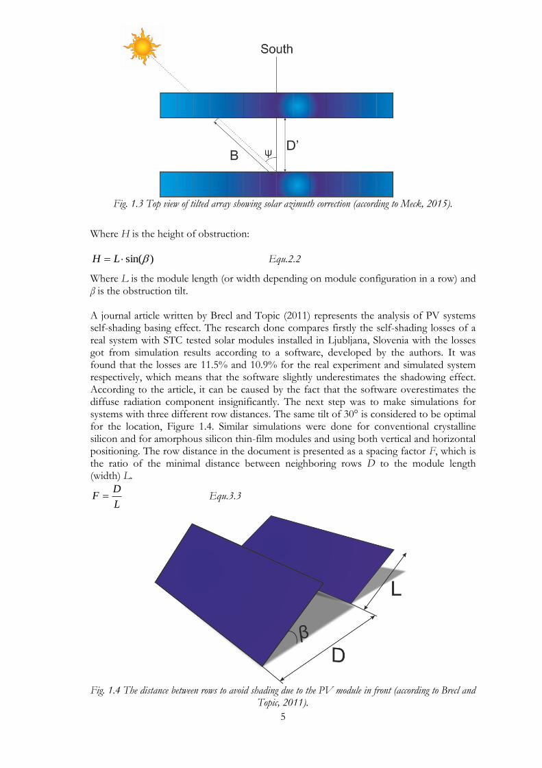
The next step is finding the sun azimuth angle ψ for the same time point, Figure 1.3. This angle represents the displacement from South of the projection of beam radiation on the horizon plane, and will be needed to obtain the minimum allowable row spacing. Both α and ψ can be found from solar calculators by entering the location coordinates and the time point for assumed solar window. Knowing the Solar Altitude and Azimuth angles minimal distance between rows D’ can be found from equation:
)180cos()tan(
'
H
D Equ.1.1
5
Fig. 1.3 Top view of tilted array showing solar azimuth correction (according to Meck, 2015).
Where H is the height of obstruction:
)sin( LH Equ.2.2
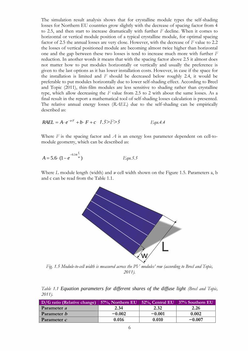
Where L is the module length (or width depending on module configuration in a row) and β is the obstruction tilt. A journal article written by Brecl and Topic (2011) represents the analysis of PV systems self-shading basing effect. The research done compares firstly the self-shading losses of a real system with STC tested solar modules installed in Ljubljana, Slovenia with the losses got from simulation results according to a software, developed by the authors. It was found that the losses are 11.5% and 10.9% for the real experiment and simulated system respectively, which means that the software slightly underestimates the shadowing effect. According to the article, it can be caused by the fact that the software overestimates the diffuse radiation component insignificantly. The next step was to make simulations for systems with three different row distances. The same tilt of 30° is considered to be optimal for the location, Figure 1.4. Similar simulations were done for conventional crystalline silicon and for amorphous silicon thin-film modules and using both vertical and horizontal positioning. The row distance in the document is presented as a spacing factor F, which is the ratio of the minimal distance between neighboring rows D to the module length (width) L.
L
DF Equ.3.3
Fig. 1.4 The distance between rows to avoid shading due to the PV module in front (according to Brecl and
Topic, 2011).
6
The simulation result analysis shows that for crystalline module types the self-shading losses for Northern EU countries grow slightly with the decrease of spacing factor from 4 to 2.5, and then start to increase dramatically with further F decline. When it comes to horizontal or vertical module position of a typical crystalline module, for optimal spacing factor of 2.5 the annual losses are very close. However, with the decrease of F value to 2.2 the losses of vertical positioned module are becoming almost twice higher than horizontal one and the gap between these two losses is tend to increase much more with further F reduction. In another words it means that with the spacing factor above 2.5 it almost does not matter how to put modules horizontally or vertically and usually the preference is given to the last options as it has lower installation costs. However, in case if the space for the installation is limited and F should be decreased below roughly 2.4, it would be preferable to put modules horizontally due to lower self-shading effect. According to Brecl and Topic (2011), thin-film modules are less sensitive to shading rather than crystalline type, which allow decreasing the F value from 2.5 to 2 with about the same losses. As a final result in the report a mathematical tool of self-shading losses calculation is presented. The relative annual energy losses (RAEL) due to the self-shading can be empirically described as:
cFbeARAEL Fa 1.5>F>5 Equ.4.4
Where F is the spacing factor and A is an energy loss parameter dependent on cell-to-module geometry, which can be described as:
)1(6.534.0
w
L
eA
Equ.5.5
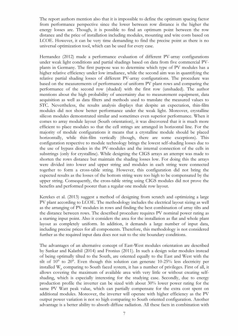
Where L module length (width) and w cell width shown on the Figure 1.5. Parameters a, b and c can be read from the Table 1.1.
Fig. 1.5 Module-to-cell width is measured across the PV modules’ row (according to Brecl and Topic,
2011).
Table 1.1 Equation parameters for different shares of the diffuse light (Brecl and Topic, 2011).
D/G ratio (Relative change) 57%, Northern EU 52%, Central EU 37% Southern EU
Parameter a 2.34 2.32 2.26
Parameter b −0.002 −0.001 0.002
Parameter c 0.016 0.010 −0.007
7
The report authors mention also that it is impossible to define the optimum spacing factor from performance perspective since the lower between row distance is the higher the energy losses are. Though, it is possible to find an optimum point between the row distance and the price of installation including modules, mounting and wire costs based on LCOE. However, it can be very time demanding to find the precise point as there is no universal optimization tool, which can be used for every case. Hernandez (2012) made a performance evaluation of different PV-array configurations under weak light conditions and partial shadings based on data from five commercial PV-plants in Germany. The first purpose was to determine which type of PV modules has a higher relative efficiency under low irradiance, while the second aim was in quantifying the relative partial shading losses of different PV-array configurations. The procedure was based on the measurements of performance of uniform PV plant rows and comparing the performance of the second row (shaded) with the first row (unshaded). The author mentions about the high probability of uncertainty due to measurement equipment, data acquisition as well as data filters and methods used to translate the measured values to STC. Nevertheless, the results analysis displays that despite an expectation, thin-film modules did not show better performance under the weak light. Moreover, crystalline silicon modules demonstrated similar and sometimes even superior performance. When it comes to array module layout (South orientation), it was discovered that it is much more efficient to place modules so that the cell strings are arranged in horizontal line. For the majority of module configurations it means that a crystalline module should be placed horizontally, while thin-film vertically (though, there are some exceptions). This configuration respective to module technology brings the lowest self-shading losses due to the use of bypass diodes in the PV-modules and the internal connection of the cells in substrings (only for crystalline). While designing the CIGS arrays an attempt was made to shorten the rows distance but maintain the shading losses low. For doing this the arrays were divided into lower and upper string and modules in each string were connected together to form a cross-table string. However, this configuration did not bring the expected results as the losses of the bottom string were too high to be compensated by the upper string. Consequently, the cross-table string using CIGS modules did not prove the benefits and performed poorer than a regular one module row layout. Kerekes et al. (2013) suggest a method of designing from scratch and optimizing a large PV plant according to LCOE. The methodology includes the electrical layout sizing as well as the arranging of PV modules in rows and finding the best combination of array tilts and the distance between rows. The described procedure requires PV nominal power rating as a starting input point. Also it considers the area for the installation as flat and whole plant layout as completely uniform. In addition, it demands a large number of input data, including precise prices for all components. Therefore, this methodology is not considered further as the required input data does not suit to the site boundary conditions. The advantages of an alternative concept of East-West modules orientation are described by Sankar and Kalathil (2014) and Fronius (2011). In such a design solar modules instead of being optimally tilted to the South, are oriented equally to the East and West with the tilt of 10° to 20°. Even though this solution can generate 10-25% less electricity per installed Wp comparing to South faced system, it has a number of privileges. First of all, it allows covering the maximum of available area with very little or without creating self-shading, which is especially interesting for the studying case. Secondly, due to energy production profile the inverter can be sized with about 30% lower power rating for the same PV Watt peak value, which can partially compensate for the extra cost spent on additional modules. Moreover, the inverter will operate with higher efficiency as the PV output power variation is not so high comparing to South oriented configuration. Another advantage is a better ability to absorb diffuse radiation. All these facts in combination with
8
proper design can make the East-West even more cost effective solution, according to the reports. Renusol (2014) explains the benefits of East-West solar installations over South oriented systems installed on flat roofs of commercial buildings in the United Kingdom. Photovoltaic installations with East-West orientation generate around 30 percent more solar power than South-facing systems fitted to flat roofs of the same size. While South-facing solar installations require their rows of modules to be spaced further apart to avoid shadows being cast by the modules and causing yield losses, in East-West installations solar modules can be fitted more tightly together on roofs often at inclinations of around ten degrees. It is also mentioned that when the feed-in tariff for grid connected systems is low, EW systems frequently prove more economically attractive. This is mainly due to the daily energy production profile, which is more consistent over the course of the day. So the larger proportion of energy consumption can be covered by solar. Being a company, which specializes on solar mounting systems, Renusol claims that since EW installations require fewer mounting materials, they incur reduced direct installation costs significantly. It is explained by better aerodynamic features and wind profile as well as shorter distance between rows. Thus, the company proposes their innovative rail-free FS10 mounting system for East-West installations, where the modules are simply secured between two foot supports and two crest supports, lessening both the cost of materials and installation time. Tröster and Schmidt (2012) studied and analyzed the performance of PV system setups with different orientations modelled for Aachen, Germany. The main motivation was that the integration of solar energy sources into already existing infrastructure may lead to less correlation of a large proportion of energy production to demand, which leads to grid overvoltage problems and a power flow into the higher voltage level. The problem of overvoltage is caused by the peak power generation of PV systems during midday. Therefore, a lower peak power would be more beneficial, which makes East-West orientation preferable from this perspective. Seven different system orientations were explored in the study, including optimal 35° South and 15° tilted East-West orientation. It was found that EW systems would produce about 13% less energy rather than South faced one considering the same system size. It should be considered that all the results have been calculated for Germany and for Sweden the advantage of the South orientation should be more pronounced according to the document. On the other hand, EW configuration daily energy production profile is wider, with lower midday peak and more production during mornings and evenings, which matches much better to typical electricity consumption profile. When it comes to annual production, the profile for June and July of the East-West option is even higher than the one of a South faced system. However, when the power is needed in the cold season, the energy output of the EW is lower. It is mentioned also that the main advantage of East-West solution is the rational usage of occupied space. Analyzing the results, authors say that there is no optimal orientation for grid operation and every PV setup has own pros and cons. Macknick et al. (2013) examine the potential of utility- and commercial-scale solar installations on degraded and environmentally contaminated areas in the USA. The main purpose of the assessment was to improve the understanding of these sites and facilitate solar developer’s selection of contaminated and disturbed sites for development. Overall, the report shows a great number of such polluted places in the country. However, the Levelized Cost of Energy is lower in the South-West of the USA, where the amount of solar radiation is the highest. The assessment addresses the subject to the fact that usually regions with such contaminated areas are predisposed to have poor economy development and a high level of unemployment. Therefore, the development of solar energy on contaminated territories can help creating work places and revitalize local and state economies. In addition, giving a priority to these sites over ordinary fields can potentially have permitting advantages and positive environmental consequences.
9
2 Background information In the following chapter, the site orientation, relief and topography, meteo data and shading profile are explained. The site is analyzed and the appropriate area for solar installation is chosen.
2.1 Boundary conditions
2.1.1. Location, orientation and relief
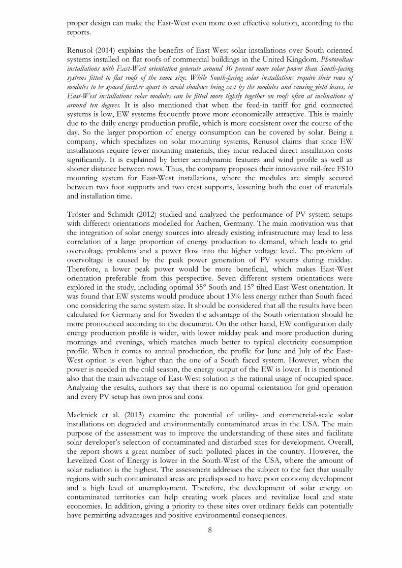
The area allotted for the installation is located in Falun, Sweden with the Latitude of 60.61°N, Longitude of 15.615°E and the Altitude of about 130m above the sea level. As can be seen from Figure 2.1 and 2.2, the territory is a field with the length of 500m from South to North and about 220m width in average from East to West, which gives approximately 110000m2 of available space in general.
Fig. 2.1 Aerial view of the studied site (Wikimapia, 2015).
The relief of the site is not uniform and has both South and North facing slopes. The last ones are undesirable for PV installation and will not be used in the design, considering the fact that there is no possibility of leveling the surface. The ground composition in the whole area is quite uniform and vegetation is practically absent. The soil is solid and reinforced with gravel and rocks.
10
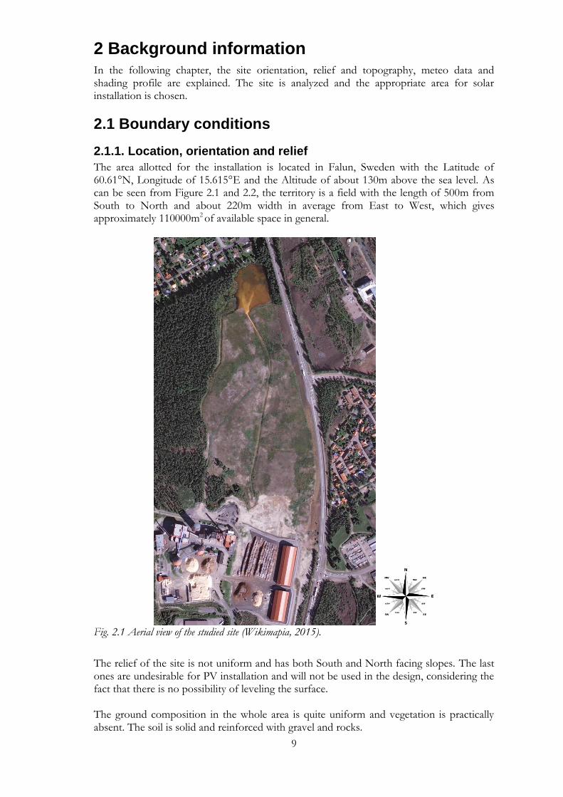
Fig. 2.2 Topographic map of the studied site (Falu Energi & Vatten, 2015).
2.1.2. Metrological data
The weather data used in the project is taken from Meteonorm (2015) for Borlänge, the neighboring city. Monthly values of global and diffuse radiation are presented in Table 2.1. For calculating the maximum voltage in the circuit it is necessary to know minimal possible daytime temperature for the place. It is assumed to be -25°C.
11
Table 2.1 Monthly Meteo values for Borlänge, Sweden (Meteonorm, 2015).
Month Jan Feb Mar Apr May Jun Jul Aug Sep Oct Nov Dec Total
Hor. Global
kWh/m2
10 28 68 108 153 163 160 122 73 33 11 6 930
Diffuse rad.
kWh/m2 6 15 31 57 71 70 76 62 38 20 8 4 456
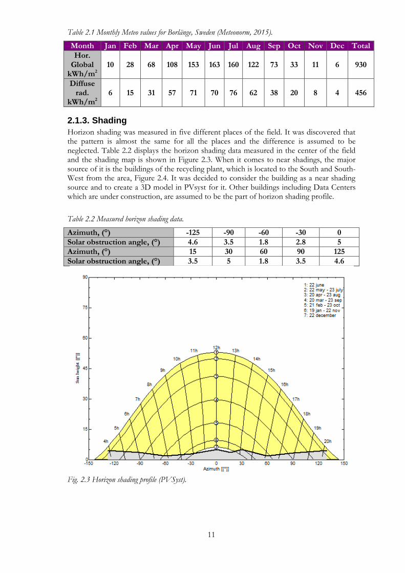
2.1.3. Shading
Horizon shading was measured in five different places of the field. It was discovered that the pattern is almost the same for all the places and the difference is assumed to be neglected. Table 2.2 displays the horizon shading data measured in the center of the field and the shading map is shown in Figure 2.3. When it comes to near shadings, the major source of it is the buildings of the recycling plant, which is located to the South and South-West from the area, Figure 2.4. It was decided to consider the building as a near shading source and to create a 3D model in PVsyst for it. Other buildings including Data Centers which are under construction, are assumed to be the part of horizon shading profile.
Table 2.2 Measured horizon shading data.
Azimuth, (°) -125 -90 -60 -30 0
Solar obstruction angle, (°) 4.6 3.5 1.8 2.8 5
Azimuth, (°) 15 30 60 90 125
Solar obstruction angle, (°) 3.5 5 1.8 3.5 4.6
Fig. 2.3 Horizon shading profile (PVSyst).
12
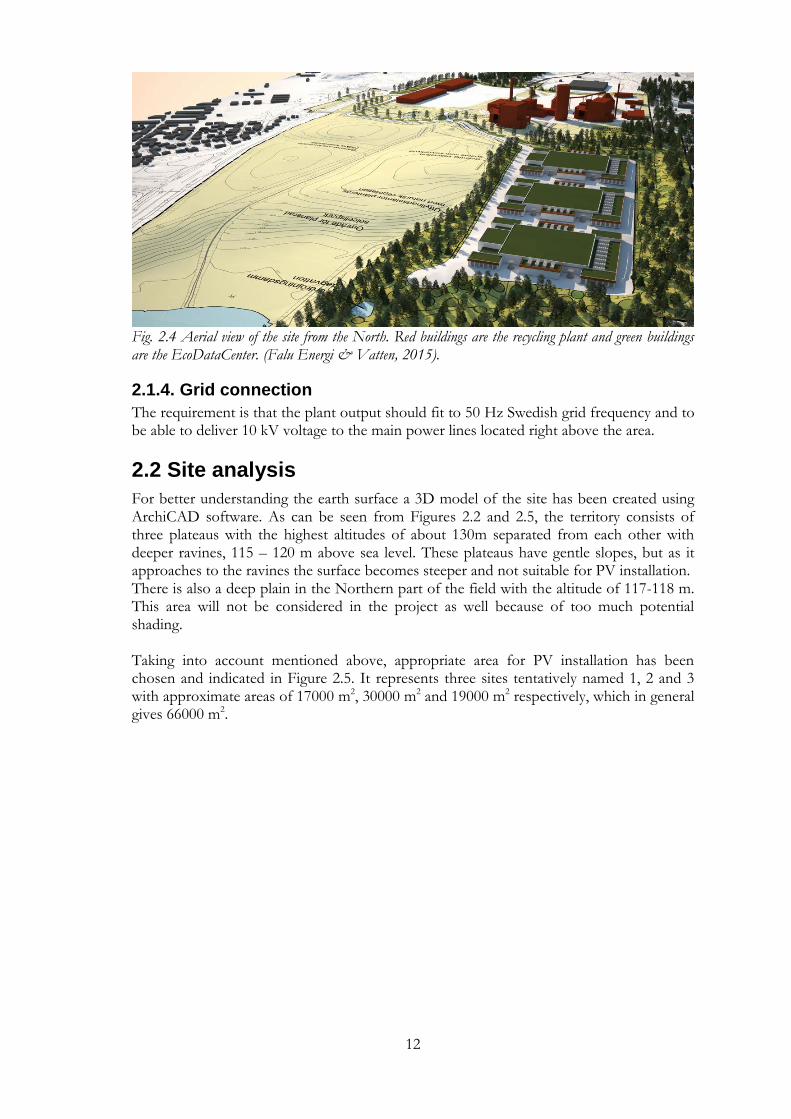
Fig. 2.4 Aerial view of the site from the North. Red buildings are the recycling plant and green buildings are the EcoDataCenter. (Falu Energi & Vatten, 2015).
2.1.4. Grid connection
The requirement is that the plant output should fit to 50 Hz Swedish grid frequency and to be able to deliver 10 kV voltage to the main power lines located right above the area.
2.2 Site analysis
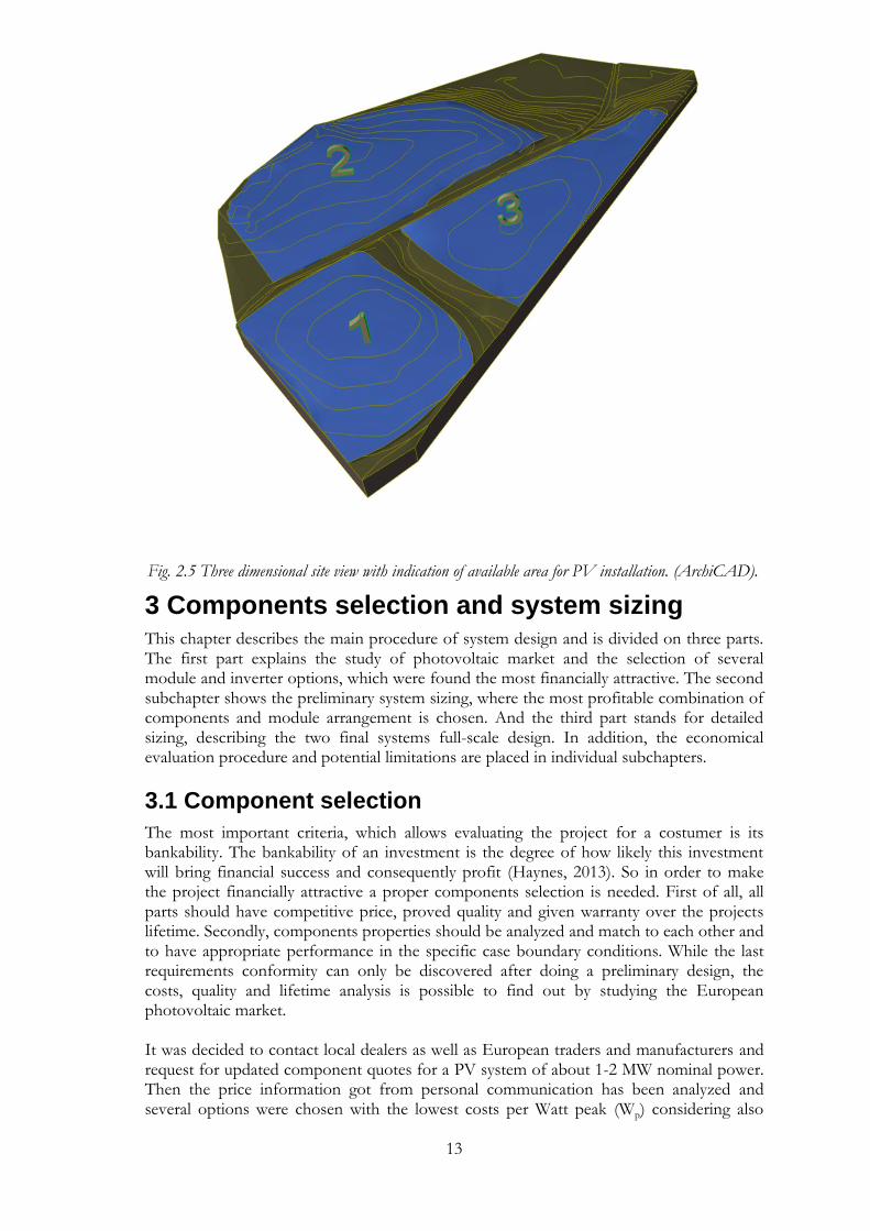
For better understanding the earth surface a 3D model of the site has been created using ArchiCAD software. As can be seen from Figures 2.2 and 2.5, the territory consists of three plateaus with the highest altitudes of about 130m separated from each other with deeper ravines, 115 – 120 m above sea level. These plateaus have gentle slopes, but as it approaches to the ravines the surface becomes steeper and not suitable for PV installation. There is also a deep plain in the Northern part of the field with the altitude of 117-118 m. This area will not be considered in the project as well because of too much potential shading. Taking into account mentioned above, appropriate area for PV installation has been chosen and indicated in Figure 2.5. It represents three sites tentatively named 1, 2 and 3 with approximate areas of 17000 m2, 30000 m2 and 19000 m2 respectively, which in general gives 66000 m2.
13
3 Components selection and system sizing This chapter describes the main procedure of system design and is divided on three parts. The first part explains the study of photovoltaic market and the selection of several module and inverter options, which were found the most financially attractive. The second subchapter shows the preliminary system sizing, where the most profitable combination of components and module arrangement is chosen. And the third part stands for detailed sizing, describing the two final systems full-scale design. In addition, the economical evaluation procedure and potential limitations are placed in individual subchapters.
3.1 Component selection
The most important criteria, which allows evaluating the project for a costumer is its bankability. The bankability of an investment is the degree of how likely this investment will bring financial success and consequently profit (Haynes, 2013). So in order to make the project financially attractive a proper components selection is needed. First of all, all parts should have competitive price, proved quality and given warranty over the projects lifetime. Secondly, components properties should be analyzed and match to each other and to have appropriate performance in the specific case boundary conditions. While the last requirements conformity can only be discovered after doing a preliminary design, the costs, quality and lifetime analysis is possible to find out by studying the European photovoltaic market. It was decided to contact local dealers as well as European traders and manufacturers and request for updated component quotes for a PV system of about 1-2 MW nominal power. Then the price information got from personal communication has been analyzed and several options were chosen with the lowest costs per Watt peak (Wp) considering also
Fig. 2.5 Three dimensional site view with indication of available area for PV installation. (ArchiCAD).
14
quality and provided warranties. Chosen components specification sheets are shown in Appendix A.
3.1.1. Modules
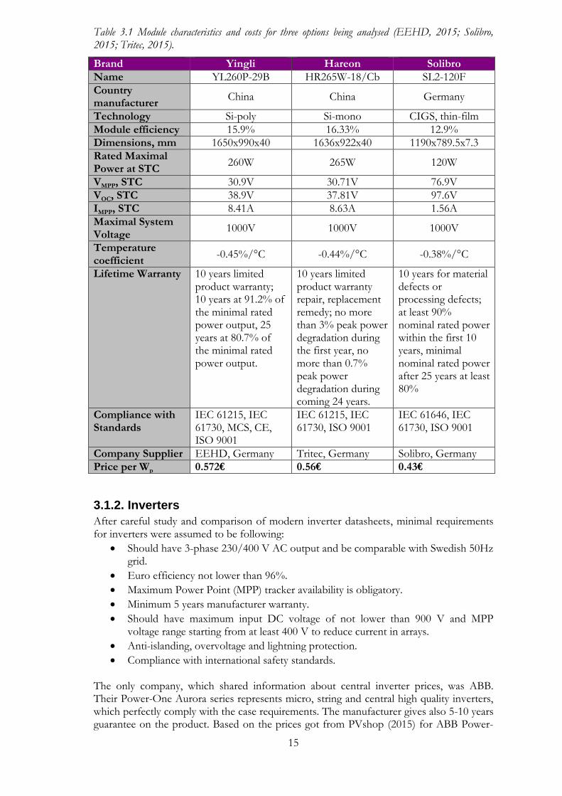
Photovoltaic modules were selected so that they meet IEC 61730 safety and IEC 61215 or IEC 61646 international standards depending on technology, crystalline or thin-film respectively. After careful study the costing information, three options were found the most financially attractive as all of them comply with the requirements and have the lowest costs per Wp among others with the same technology. Main characteristics and costs for the three chosen modules are presented in Table 3.1.
1. Yingli YL260P-29B Being one of the top worldwide module manufacturers, Yingli provides a high quality product for reasonable price. These particular modules are 60 cell silicon polycrystalline (Si-poly) 260 W modules with 15.9% efficiency. They have tight and positive power tolerance of 0 to +5 W. It guaranties the modules to perform at or above nameplate power and contributes to minimizing module mismatch losses, which leads to improved system yield.
2. Hareon HR265W-18/Cb These are silicon monocrystalline (Si-mono) modules, with 265 W nominal power. The selection of these modules was based on their low costs and relatively high efficiency of 16.33%. Despite the fact that Hareon is relatively new on the solar market, their production meets all the necessary international standards. The company provides also an attractive warranty for their product. Moreover, these modules are available and in stock on European market.
3. Solibro SL2-120F Unlike previous ones, Solibro uses CIGS thin-film technology in their modules. This implies lower efficiency (12.9%), but lower costs per Wp on the other hand. Thus, the
choice is motivated by the most attractive price of 0.43 €/ Wp. In addition, thin-film panels have better temperature coefficient and higher output voltage, which might lead to a system losses decrease. It should be also considered that those modules are frameless and require special mounting. The modules are produced in Germany, while the developing department is located in Uppsala, Sweden. Therefore, it can have a positive effect on project branding and advertisement.
15
Table 3.1 Module characteristics and costs for three options being analysed (EEHD, 2015; Solibro, 2015; Tritec, 2015).
Brand Yingli Hareon Solibro
Name YL260P-29B HR265W-18/Cb SL2-120F
Country manufacturer
China China Germany
Technology Si-poly Si-mono CIGS, thin-film
Module efficiency 15.9% 16.33% 12.9%
Dimensions, mm 1650x990x40 1636x922x40 1190x789.5x7.3
Rated Maximal Power at STC
260W 265W 120W
VMPP, STC 30.9V 30.71V 76.9V
VOC, STC 38.9V 37.81V 97.6V
IMPP, STC 8.41A 8.63A 1.56A
Maximal System Voltage
1000V 1000V 1000V
Temperature coefficient
-0.45%/°C -0.44%/°C -0.38%/°C
Lifetime Warranty 10 years limited product warranty; 10 years at 91.2% of the minimal rated power output, 25 years at 80.7% of the minimal rated power output.
10 years limited product warranty repair, replacement remedy; no more than 3% peak power degradation during the first year, no more than 0.7% peak power degradation during coming 24 years.
10 years for material defects or processing defects; at least 90% nominal rated power within the first 10 years, minimal nominal rated power after 25 years at least 80%
Compliance with Standards
IEC 61215, IEC 61730, MCS, CE, ISO 9001
IEC 61215, IEC 61730, ISO 9001
IEC 61646, IEC 61730, ISO 9001
Company Supplier EEHD, Germany Tritec, Germany Solibro, Germany
Price per Wp 0.572€ 0.56€ 0.43€
3.1.2. Inverters
After careful study and comparison of modern inverter datasheets, minimal requirements for inverters were assumed to be following:
Should have 3-phase 230/400 V AC output and be comparable with Swedish 50Hz grid.
Euro efficiency not lower than 96%.
Maximum Power Point (MPP) tracker availability is obligatory.
Minimum 5 years manufacturer warranty.
Should have maximum input DC voltage of not lower than 900 V and MPP voltage range starting from at least 400 V to reduce current in arrays.
Anti-islanding, overvoltage and lightning protection.
Compliance with international safety standards.
The only company, which shared information about central inverter prices, was ABB. Their Power-One Aurora series represents micro, string and central high quality inverters, which perfectly comply with the case requirements. The manufacturer gives also 5-10 years guarantee on the product. Based on the prices got from PVshop (2015) for ABB Power-
16
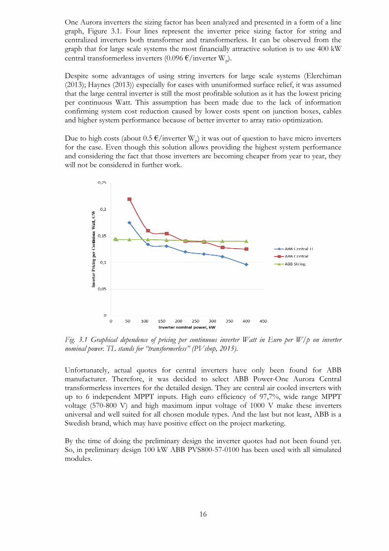
One Aurora inverters the sizing factor has been analyzed and presented in a form of a line graph, Figure 3.1. Four lines represent the inverter price sizing factor for string and centralized inverters both transformer and transformerless. It can be observed from the graph that for large scale systems the most financially attractive solution is to use 400 kW
central transformerless inverters (0.096 €/inverter Wp). Despite some advantages of using string inverters for large scale systems (Elerchiman (2013); Haynes (2013)) especially for cases with ununiformed surface relief, it was assumed that the large central inverter is still the most profitable solution as it has the lowest pricing per continuous Watt. This assumption has been made due to the lack of information confirming system cost reduction caused by lower costs spent on junction boxes, cables and higher system performance because of better inverter to array ratio optimization.
Due to high costs (about 0.5 €/inverter Wp) it was out of question to have micro inverters for the case. Even though this solution allows providing the highest system performance and considering the fact that those inverters are becoming cheaper from year to year, they will not be considered in further work.
Fig. 3.1 Graphical dependence of pricing per continuous inverter Watt in Euro per W/p on inverter nominal power. TL stands for “transformerless” (PVshop, 2015).
Unfortunately, actual quotes for central inverters have only been found for ABB manufacturer. Therefore, it was decided to select ABB Power-One Aurora Central transformerless inverters for the detailed design. They are central air cooled inverters with up to 6 independent MPPT inputs. High euro efficiency of 97,7%, wide range MPPT voltage (570-800 V) and high maximum input voltage of 1000 V make these inverters universal and well suited for all chosen module types. And the last but not least, ABB is a Swedish brand, which may have positive effect on the project marketing. By the time of doing the preliminary design the inverter quotes had not been found yet. So, in preliminary design 100 kW ABB PVS800-57-0100 has been used with all simulated modules.

17
Table 3.2 Prices of inverters considered in the design (based on prices got from PVshop (2015)).
Inverter name Rated power Price
ABB PVS800-57-0100 100 kW 14000 €
ABB Power-One Aurora PVI-400-TL 400 kW 38379 €
3.1.3. Mounting and other electrical components
Mounting include components, which are basically responsible for fixing modules on the surface, while other electrical components stand for cables, junction boxes, fuses, etc. An assumption had to be made here as well because none of contacted companies shared the price information. The decided approximate quotes are based on cost figures provided by the university. Nevertheless, from personal communication with photovoltaic designer companies it was found out that some corrections should be made to these figures, Table 3.3, 3.4. Regarding racking, as piling is not allowed, it is reasonable to apply “swimming” type of mounting where extra concrete weight is attached to construction so it can stand high winds and storms. By itself this type of construction might not be much different in price from typical piled installation. However, this solution should cause significant mounting cost reduction for East-West module arrangement, which is also considered. Such mounting system will have extremely low wind profile due to very low height and tilt. Consequently less concrete is needed, which in turn will positively affect the price. It means that mounting costs cannot have the same relation to PV nominal power for South and East-West design. A limitation should be commented, which was used for electrical components price. It was assumed that the difference in cable price change is negligible for different variations of row to row distance. It was also decided to assume constant electrical components price to PV nominal power ratio no matter what type of inverter was used in simulations.
Table 3.3 Cost figures for PV mounting system in Euro/Wp, according to PV nominal power (based on cost estimated figures got from PV design course in Dalarna University).
Type of mounting system Cost figures according to PV nominal power
Mounting Si-mono 0.14 €/Wp
Mounting Si-poly 0.15 €/Wp
Mounting Thin-Film South orientation 0.18 €/Wp
Mounting Thin-Film East-West orientation 0.14 €/Wp
Table 3.4 Cost figures for PV Balance Of System components as a share of total equipment costs, % (based on cost estimated figures got from PV design course in Dalarna University).
Cost categories Cost share according to total equipment costs
Electrical components (wires, cables, junction boxes) 0.1%
Installation (work) 0.15%
Component shipping 0.02%
Engineering margin South orientation 0.05%
3.2 Preliminary sizing
By doing the preliminary design it was aimed to explore and evaluate the performance of different modules based on their bankability and to analyze the system performance with various tilts, row spacing factor and orientation. The best results from this section will be
18
used as a starting point for further detailed design. Therefore, for all cases the same 100 kW central inverter is being considered in order to make a fair and clear comparison between various options. As there are many variable parameters affecting final system performance and LCOE it was agreed to follow the next procedure. First of all, the system electrical layout should be designed, which includes strings sizing and numbering. For doing this optimized row spacing factor and tilt were used, suggested by PVsyst. Then a number of simulations were done by varying the row distance and finding optimal tilt for each meter of the distance by defining maximal system annual power production for each distance. The procedure was repeated for all three module types. Besides South system orientation, simulations were done for East-West module arrangement. For this option thin-film Solibro modules were chosen only as the best price solution. After this, for each simulation result economic evaluation was made based on Levelized Cost of Energy (LCOE) and total costs per annual power production value calculation described in Chapter 3.4. Then the results were analyzed and several most financially attractive options were chosen for detailed design. All simulations were done in PVsyst program (PVsyst, 2015). Perez-Ineichen model was chosen, which is assumed to be better for Swedish climate as it is more precise for diffuse irradiation component. Constant albedo of 0.2 was used. Electrical shading effect was enabled.
3.2.1. String sizing and numbering
The first step in selecting the number of modules connected in series in a string was to define the lowest possible temperature for absolute voltage limit, which constitutes -25°C. This temperature has been decided based on estimation made after studying the weather data for the location. Though, the lowest ambient temperature can easily reach -30°, it is only possible during night, when there is no sunlight for module operation. Then according to this extreme temperature it was possible to calculate maximum open circuit voltage for all modules for the location:
)100
) 25°C) - ((T + (1 V =V mod
oc MAXTK
Equ.3.1.
Where VMAX - Maximum photovoltaic module output voltage; VOC - Module open circuit voltage; TMOD - Lowest possible module temperature during day, (-25°C);
TK - Module temperature coefficient.
From this adjusted maximum voltage the highest possible number of modules in string was found. It was done by dividing the maximum input inverter voltage (1000 V) by VMAX value and rounding to the nearest whole number. The results of these calculations are presented in Table 3.3. In fact, this simple calculation is usually done in PVsyst program, but it is highly recommended to repeat it manually to be ensured of preventing system overvoltage.
Table 3.5 Maximum possible module output voltage for the location and maximum number of module in strings considering 1000 V as the highest allowable inverter input voltage.
Module Yingli Hareon Solibro
VMAX at -25°C 47.6 V 46.4 V 116.1 V
Max. number of modules in string for 1000V 20 20 8
Selected number of modules in series for preliminary design
19 19 7
19
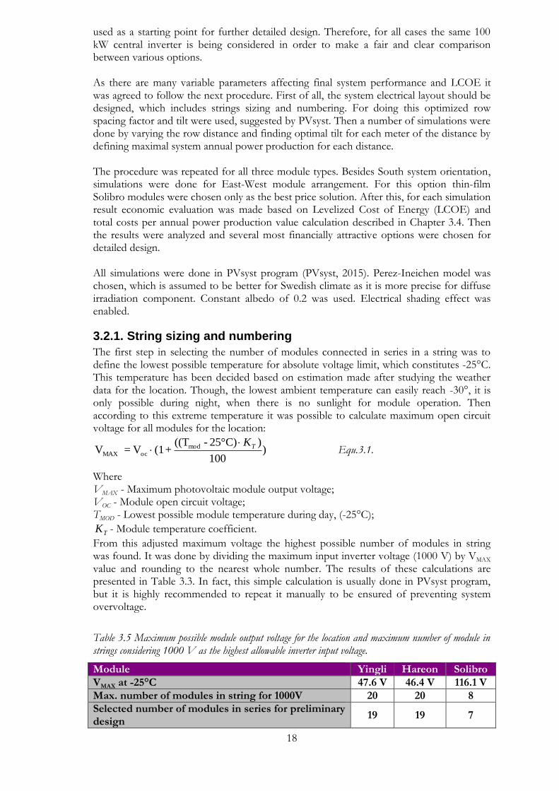
Further string sizing procedure was based on finding maximum suitable module number so that module MPP voltage at operating temperature (10-50°C) suits to inverter MPP voltage range. This calculation procedure is automated and done by PVsyst software. As the MPP voltage gap of the inverter is quite wide (from 425 V to 850 V), there are several options of possible module number in a string, from 18 to 20 for crystalline and from 7 to 8 for thin-film modules. According to inverter efficiency data (Figure 3.2) the inverter performs better in lower voltage conditions. On the other hand, the higher system voltage is the lower current for the same delivered power. Consequently, lower losses and less money should be spent on cables. So it was decided for preliminary design to choose the middle option of 19 and 7 modules for crystalline and thin-film modules respectively, as a compromise between inverter efficiency and cable costs.
Fig. 3.2 Efficiency curves of 100kW ABB inverter chosen for preliminary design. Blue, green and red
curves represent the efficiency for 800 V, 600 V and 450 V input DC voltage (PVsyst).
After selecting the optimal string size the string number in parallel should be found. Here the main criterion was module/inverter power ratio. This value can be found by dividing PV array nominal power by inverter nominal power. Typically this value varies between 0.85-1.26 depending on system boundary conditions. Taking into account that module nominal power is defined for Standard Test Conditions (STC, irradiation 1000 W/m² and module temperature 25°C), such PV power can never or very rarely be attained for the site in reality. Therefore, it is reasonable to consider undersized inverter for the case. A series of simulations have been done varying this ratio by changing the number of module strings and then evaluating the system bankability based on Levelized Cost of Energy on annual basis (according to Chapter 3.4). Consequently, it was assumed in preliminary design to keep the module/inverter power ratio in range of 1.23-1.4 for South orientation, as a compromise between system performance and bankability. When it comes to East-West orientation, the same procedure has been used. The main difference is that in this case 2 MPPT inputs of inverter were independently involved in simulations, one for East and another for West orientation. As in this case modules generate less electricity, the nominal power ratio is higher, 1.6 and 1.55 for East and West respectively. The difference is due to weather data, horizon shading profile and the module operating temperature, which will always be lower in the first part of the day. As a result, final numbers of strings and modules have been found and indicated in Table 3.4. System losses due to inverter undersizing (overload) are also called as acceptable overload losses and are presented as a sizing result in PVsyst. The meaning of the loss is to show how much of possible energy production will be lost because of undersized inverter.
20
Table 3.6 Chosen string numbering parameters for preliminary design. Systems with different modules and orientation and the same 100 kW inverter.
Orientation South East-West
Module Yingli Hareon Solibro Solibro
Module/inverter power ratio 1.28 1.26 1.27 1.55-1.6
Losses due to inverter overload 0.5% 0.4% 0.5% 0.5%
Number of strings 26 25 151 187
Total number of modules 494 475 1057 1309
PV nominal power 128 kWp 126 kWp 127 kWp 157 kWp
3.2.2. Row spacing factor and tilt
One of the most important parameters to consider when designing a utility-scale photovoltaic system are module tilt and the distance between rows. So it has been paid a special attention for these values optimization, presented in this subchapter. Typically in the Northern hemisphere it is recommended to install solar panels facing the South, being an optimal orientation solution. However, there are certain advantages of East-West orientation as well, so both of these designs are considered and individually described below.
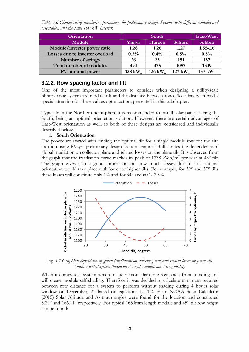
1. South Orientation The procedure started with finding the optimal tilt for a single module row for the site location using PVsyst preliminary design section. Figure 3.3 illustrates the dependence of global irradiation on collector plane and related losses on the plane tilt. It is observed from the graph that the irradiation curve reaches its peak of 1238 kWh/m2 per year at 48° tilt. The graph gives also a good impression on how much losses due to not optimal orientation would take place with lower or higher tilts. For example, for 39° and 57° tilts these losses will constitute only 1% and for 34° and 60° - 2.5%.
Fig. 3.3 Graphical dependence of global irradiation on collector plane and related losses on plane tilt.
South oriented system (based on PVsyst simulations, Perez model).
When it comes to a system which includes more than one row, each front standing line will create module self-shading. Therefore it was decided to calculate minimum required between row distance for a system to perform without shading during 4 hours solar window on December, 21 based on equations 1.1-1.2. From NOAA Solar Calculator (2015) Solar Altitude and Azimuth angles were found for the location and constituted 5.22° and 166.11° respectively. For typical 1650mm length module and 45° tilt row height can be found:
21
mH 167.1)45sin(65.1 Equ.3.1
Between row distance:
mD 4.12)11.166180cos()22.5tan(
167.1 Equ.3.2
This distance was assumed to be maximal and was used in further procedure as a starting point describing approximate distance without losses. It is obvious that with the increase of row distance system will have higher power production due to less shading. However, it is not reasonable to have the distance higher than 12.4 m as it would decrease area occupation factor and the system will have low nominal power per meter of ground. Ground area occupation ratio is a unitless value and is mathematically described as:
GROUND
COLLOCCUP
A
AF Equ.3.3
Where
COLLA - Total collector gross area;
GROUNDA - The area of ground occupied by the plant.
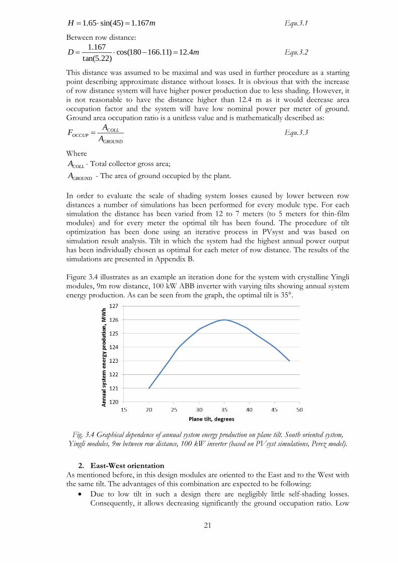
In order to evaluate the scale of shading system losses caused by lower between row distances a number of simulations has been performed for every module type. For each simulation the distance has been varied from 12 to 7 meters (to 5 meters for thin-film modules) and for every meter the optimal tilt has been found. The procedure of tilt optimization has been done using an iterative process in PVsyst and was based on simulation result analysis. Tilt in which the system had the highest annual power output has been individually chosen as optimal for each meter of row distance. The results of the simulations are presented in Appendix B. Figure 3.4 illustrates as an example an iteration done for the system with crystalline Yingli modules, 9m row distance, 100 kW ABB inverter with varying tilts showing annual system energy production. As can be seen from the graph, the optimal tilt is 35°.
Fig. 3.4 Graphical dependence of annual system energy production on plane tilt. South oriented system,
Yingli modules, 9m between row distance, 100 kW inverter (based on PVsyst simulations, Perez model).
2. East-West orientation
As mentioned before, in this design modules are oriented to the East and to the West with the same tilt. The advantages of this combination are expected to be following:
Due to low tilt in such a design there are negligibly little self-shading losses. Consequently, it allows decreasing significantly the ground occupation ratio. Low
22
tilt contributes also to better ability to absorb diffuse radiation, which is topical for cloudy Swedish weather conditions.
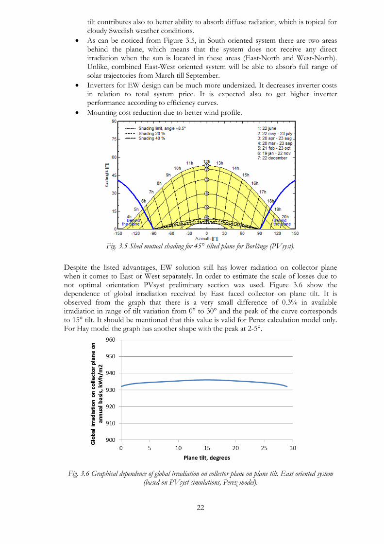
As can be noticed from Figure 3.5, in South oriented system there are two areas behind the plane, which means that the system does not receive any direct irradiation when the sun is located in these areas (East-North and West-North). Unlike, combined East-West oriented system will be able to absorb full range of solar trajectories from March till September.
Inverters for EW design can be much more undersized. It decreases inverter costs in relation to total system price. It is expected also to get higher inverter performance according to efficiency curves.
Mounting cost reduction due to better wind profile.
Fig. 3.5 Shed mutual shading for 45° tilted plane for Borlänge (PVsyst).
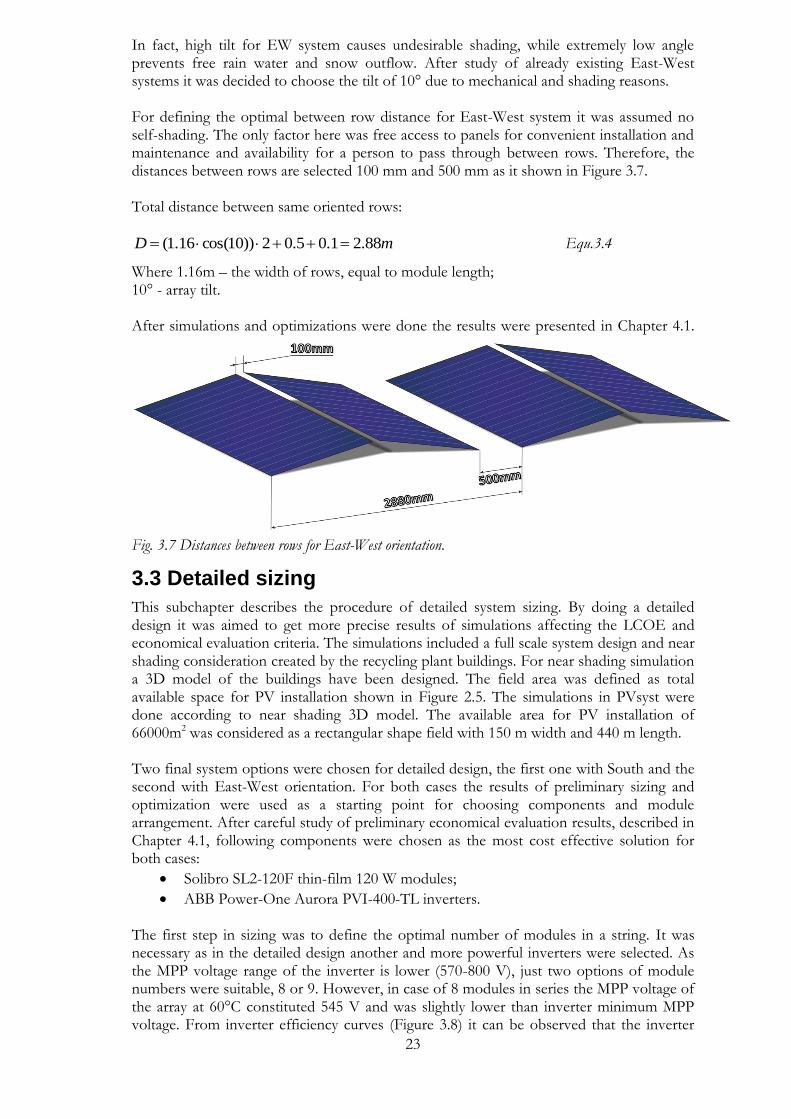
Despite the listed advantages, EW solution still has lower radiation on collector plane when it comes to East or West separately. In order to estimate the scale of losses due to not optimal orientation PVsyst preliminary section was used. Figure 3.6 show the dependence of global irradiation received by East faced collector on plane tilt. It is observed from the graph that there is a very small difference of 0.3% in available irradiation in range of tilt variation from 0° to 30° and the peak of the curve corresponds to 15° tilt. It should be mentioned that this value is valid for Perez calculation model only. For Hay model the graph has another shape with the peak at 2-5°.
Fig. 3.6 Graphical dependence of global irradiation on collector plane on plane tilt. East oriented system
(based on PVsyst simulations, Perez model).
23
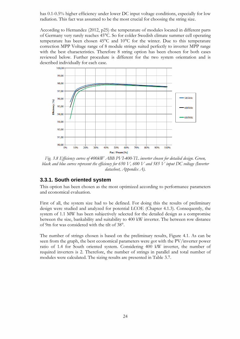
In fact, high tilt for EW system causes undesirable shading, while extremely low angle prevents free rain water and snow outflow. After study of already existing East-West systems it was decided to choose the tilt of 10° due to mechanical and shading reasons. For defining the optimal between row distance for East-West system it was assumed no self-shading. The only factor here was free access to panels for convenient installation and maintenance and availability for a person to pass through between rows. Therefore, the distances between rows are selected 100 mm and 500 mm as it shown in Figure 3.7. Total distance between same oriented rows:
mD 88.21.05.02))10cos(16.1( Equ.3.4
Where 1.16m – the width of rows, equal to module length; 10° - array tilt. After simulations and optimizations were done the results were presented in Chapter 4.1.
3.3 Detailed sizing
This subchapter describes the procedure of detailed system sizing. By doing a detailed design it was aimed to get more precise results of simulations affecting the LCOE and economical evaluation criteria. The simulations included a full scale system design and near shading consideration created by the recycling plant buildings. For near shading simulation a 3D model of the buildings have been designed. The field area was defined as total available space for PV installation shown in Figure 2.5. The simulations in PVsyst were done according to near shading 3D model. The available area for PV installation of 66000m2 was considered as a rectangular shape field with 150 m width and 440 m length. Two final system options were chosen for detailed design, the first one with South and the second with East-West orientation. For both cases the results of preliminary sizing and optimization were used as a starting point for choosing components and module arrangement. After careful study of preliminary economical evaluation results, described in Chapter 4.1, following components were chosen as the most cost effective solution for both cases:
Solibro SL2-120F thin-film 120 W modules;
ABB Power-One Aurora PVI-400-TL inverters.
The first step in sizing was to define the optimal number of modules in a string. It was necessary as in the detailed design another and more powerful inverters were selected. As the MPP voltage range of the inverter is lower (570-800 V), just two options of module numbers were suitable, 8 or 9. However, in case of 8 modules in series the MPP voltage of the array at 60°C constituted 545 V and was slightly lower than inverter minimum MPP voltage. From inverter efficiency curves (Figure 3.8) it can be observed that the inverter
Fig. 3.7 Distances between rows for East-West orientation.
24
has 0.1-0.5% higher efficiency under lower DC input voltage conditions, especially for low radiation. This fact was assumed to be the most crucial for choosing the string size. According to Hernandez (2012, p25) the temperature of modules located in different parts of Germany very rarely reaches 45°C. So for colder Swedish climate summer cell operating temperature has been chosen 45°C and 10°C for the winter. Due to this temperature correction MPP Voltage range of 8 module strings suited perfectly to inverter MPP range with the best characteristics. Therefore 8 string option has been chosen for both cases reviewed below. Further procedure is different for the two system orientation and is described individually for each case.
Fig. 3.8 Efficiency curves of 400kW ABB PVI-400-TL inverter chosen for detailed design. Green,
black and blue curves represent the efficiency for 650 V, 600 V and 585 V input DC voltage (Inverter datasheet, Appendix A).
3.3.1. South oriented system
This option has been chosen as the most optimized according to performance parameters and economical evaluation. First of all, the system size had to be defined. For doing this the results of preliminary design were studied and analyzed for potential LCOE (Chapter 4.1.3). Consequently, the system of 1.1 MW has been subjectively selected for the detailed design as a compromise between the size, bankability and suitability to 400 kW inverter. The between row distance of 9m for was considered with the tilt of 38°. The number of strings chosen is based on the preliminary results, Figure 4.1. As can be seen from the graph, the best economical parameters were got with the PV/inverter power ratio of 1.4 for South oriented system. Considering 400 kW inverter, the number of required inverters is 2. Therefore, the number of strings in parallel and total number of modules were calculated. The sizing results are presented in Table 3.7.
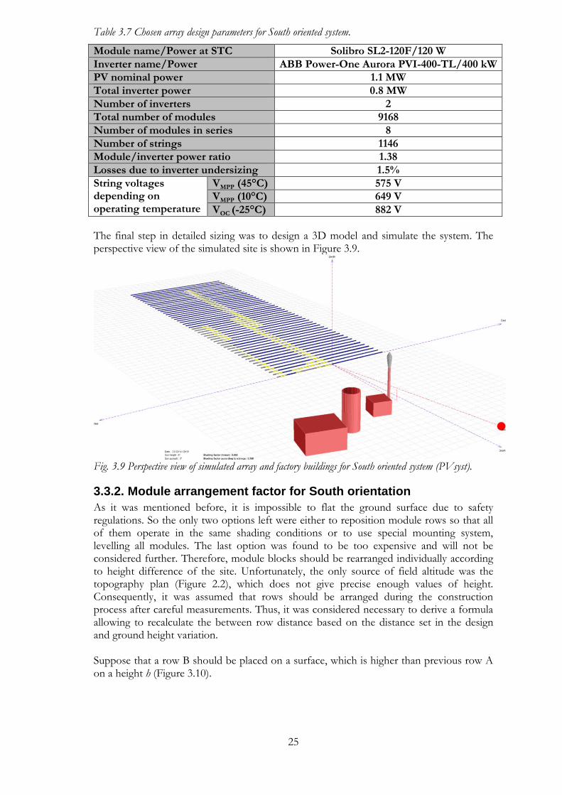
25
Table 3.7 Chosen array design parameters for South oriented system.
Module name/Power at STC Solibro SL2-120F/120 W
Inverter name/Power ABB Power-One Aurora PVI-400-TL/400 kW
PV nominal power 1.1 MW
Total inverter power 0.8 MW
Number of inverters 2
Total number of modules 9168
Number of modules in series 8
Number of strings 1146
Module/inverter power ratio 1.38
Losses due to inverter undersizing 1.5%
String voltages depending on operating temperature
VMPP (45°C) 575 V
VMPP (10°C) 649 V
VOC (-25°C) 882 V
The final step in detailed sizing was to design a 3D model and simulate the system. The perspective view of the simulated site is shown in Figure 3.9.
Fig. 3.9 Perspective view of simulated array and factory buildings for South oriented system (PVsyst).
3.3.2. Module arrangement factor for South orientation
As it was mentioned before, it is impossible to flat the ground surface due to safety regulations. So the only two options left were either to reposition module rows so that all of them operate in the same shading conditions or to use special mounting system, levelling all modules. The last option was found to be too expensive and will not be considered further. Therefore, module blocks should be rearranged individually according to height difference of the site. Unfortunately, the only source of field altitude was the topography plan (Figure 2.2), which does not give precise enough values of height. Consequently, it was assumed that rows should be arranged during the construction process after careful measurements. Thus, it was considered necessary to derive a formula allowing to recalculate the between row distance based on the distance set in the design and ground height variation. Suppose that a row B should be placed on a surface, which is higher than previous row A on a height h (Figure 3.10).
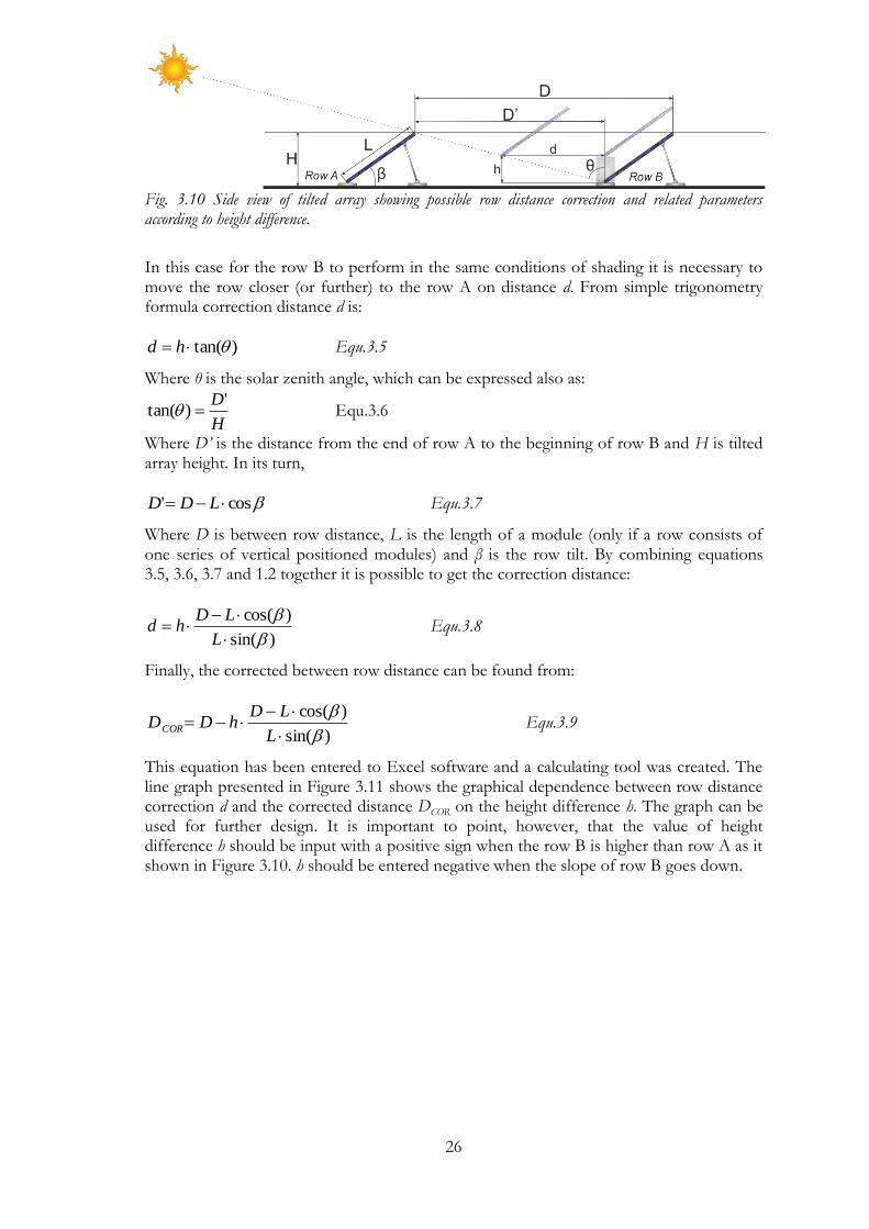
26
Fig. 3.10 Side view of tilted array showing possible row distance correction and related parameters according to height difference.
In this case for the row B to perform in the same conditions of shading it is necessary to move the row closer (or further) to the row A on distance d. From simple trigonometry formula correction distance d is:
)tan( hd Equ.3.5
Where θ is the solar zenith angle, which can be expressed also as:
H
D')tan( Equ.3.6
Where D’ is the distance from the end of row A to the beginning of row B and H is tilted array height. In its turn,
cos' LDD Equ.3.7
Where D is between row distance, L is the length of a module (only if a row consists of one series of vertical positioned modules) and β is the row tilt. By combining equations 3.5, 3.6, 3.7 and 1.2 together it is possible to get the correction distance:
)sin(
)cos(
L
LDhd Equ.3.8
Finally, the corrected between row distance can be found from:
)sin(
)cos(
L
LDhDDCOR Equ.3.9
This equation has been entered to Excel software and a calculating tool was created. The line graph presented in Figure 3.11 shows the graphical dependence between row distance correction d and the corrected distance DCOR on the height difference h. The graph can be used for further design. It is important to point, however, that the value of height difference h should be input with a positive sign when the row B is higher than row A as it shown in Figure 3.10. h should be entered negative when the slope of row B goes down.
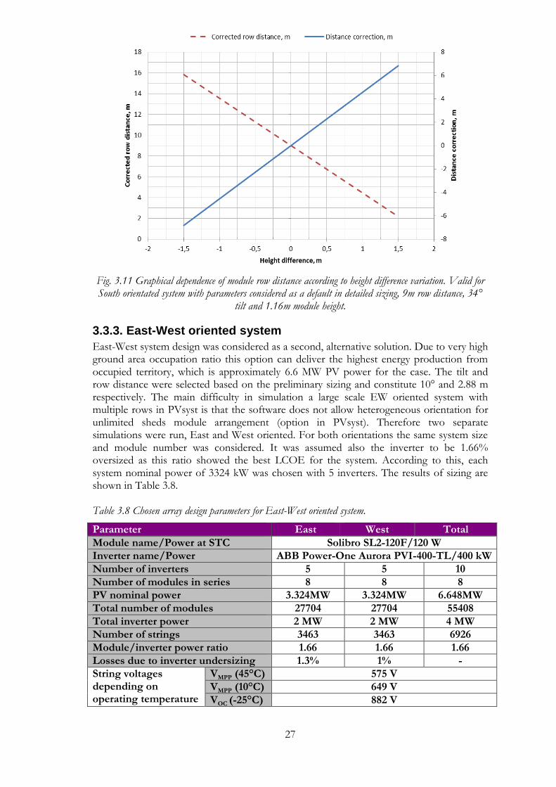
27
Fig. 3.11 Graphical dependence of module row distance according to height difference variation. Valid for South orientated system with parameters considered as a default in detailed sizing, 9m row distance, 34°
tilt and 1.16m module height.
3.3.3. East-West oriented system
East-West system design was considered as a second, alternative solution. Due to very high ground area occupation ratio this option can deliver the highest energy production from occupied territory, which is approximately 6.6 MW PV power for the case. The tilt and row distance were selected based on the preliminary sizing and constitute 10° and 2.88 m respectively. The main difficulty in simulation a large scale EW oriented system with multiple rows in PVsyst is that the software does not allow heterogeneous orientation for unlimited sheds module arrangement (option in PVsyst). Therefore two separate simulations were run, East and West oriented. For both orientations the same system size and module number was considered. It was assumed also the inverter to be 1.66% oversized as this ratio showed the best LCOE for the system. According to this, each system nominal power of 3324 kW was chosen with 5 inverters. The results of sizing are shown in Table 3.8. Table 3.8 Chosen array design parameters for East-West oriented system.
Parameter East West Total
Module name/Power at STC Solibro SL2-120F/120 W
Inverter name/Power ABB Power-One Aurora PVI-400-TL/400 kW
Number of inverters 5 5 10
Number of modules in series 8 8 8
PV nominal power 3.324MW 3.324MW 6.648MW
Total number of modules 27704 27704 55408
Total inverter power 2 MW 2 MW 4 MW
Number of strings 3463 3463 6926
Module/inverter power ratio 1.66 1.66 1.66
Losses due to inverter undersizing 1.3% 1% -
String voltages depending on operating temperature
VMPP (45°C) 575 V
VMPP (10°C) 649 V
VOC (-25°C) 882 V
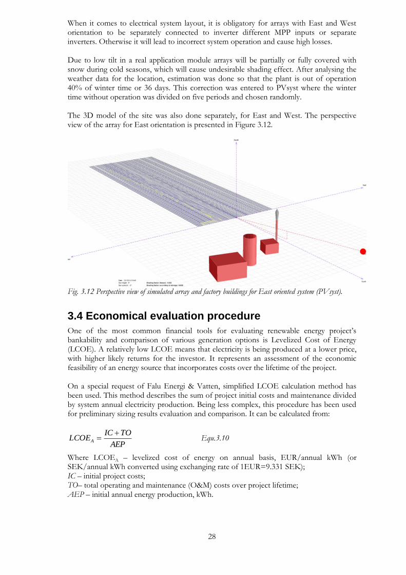
28
When it comes to electrical system layout, it is obligatory for arrays with East and West orientation to be separately connected to inverter different MPP inputs or separate inverters. Otherwise it will lead to incorrect system operation and cause high losses. Due to low tilt in a real application module arrays will be partially or fully covered with snow during cold seasons, which will cause undesirable shading effect. After analysing the weather data for the location, estimation was done so that the plant is out of operation 40% of winter time or 36 days. This correction was entered to PVsyst where the winter time without operation was divided on five periods and chosen randomly. The 3D model of the site was also done separately, for East and West. The perspective view of the array for East orientation is presented in Figure 3.12.
Fig. 3.12 Perspective view of simulated array and factory buildings for East oriented system (PVsyst).
3.4 Economical evaluation procedure
One of the most common financial tools for evaluating renewable energy project’s bankability and comparison of various generation options is Levelized Cost of Energy (LCOE). A relatively low LCOE means that electricity is being produced at a lower price, with higher likely returns for the investor. It represents an assessment of the economic feasibility of an energy source that incorporates costs over the lifetime of the project. On a special request of Falu Energi & Vatten, simplified LCOE calculation method has been used. This method describes the sum of project initial costs and maintenance divided by system annual electricity production. Being less complex, this procedure has been used for preliminary sizing results evaluation and comparison. It can be calculated from:
AEP
TOICLCOEA
Equ.3.10
Where LCOEA – levelized cost of energy on annual basis, EUR/annual kWh (or SEK/annual kWh converted using exchanging rate of 1EUR=9.331 SEK); IC – initial project costs; TO– total operating and maintenance (O&M) costs over project lifetime; AEP – initial annual energy production, kWh.
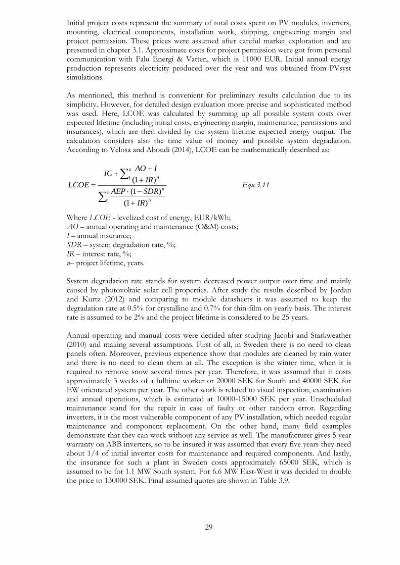
29
Initial project costs represent the summary of total costs spent on PV modules, inverters, mounting, electrical components, installation work, shipping, engineering margin and project permission. These prices were assumed after careful market exploration and are presented in chapter 3.1. Approximate costs for project permission were got from personal communication with Falu Energi & Vatten, which is 11000 EUR. Initial annual energy production represents electricity produced over the year and was obtained from PVsyst simulations. As mentioned, this method is convenient for preliminary results calculation due to its simplicity. However, for detailed design evaluation more precise and sophisticated method was used. Here, LCOE was calculated by summing up all possible system costs over expected lifetime (including initial costs, engineering margin, maintenance, permissions and insurances), which are then divided by the system lifetime expected energy output. The calculation considers also the time value of money and possible system degradation. According to Velosa and Aboudi (2014), LCOE can be mathematically described as:
n
n
n
n
n
IR
SDRAEP
IR
IAOIC
LCOE
1
1
)1(
)1(
)1( Equ.3.11
Where LCOE - levelized cost of energy, EUR/kWh; AO – annual operating and maintenance (O&M) costs; I – annual insurance; SDR – system degradation rate, %; IR – interest rate, %; n– project lifetime, years. System degradation rate stands for system decreased power output over time and mainly caused by photovoltaic solar cell properties. After study the results described by Jordan and Kurtz (2012) and comparing to module datasheets it was assumed to keep the degradation rate at 0.5% for crystalline and 0.7% for thin-film on yearly basis. The interest rate is assumed to be 2% and the project lifetime is considered to be 25 years. Annual operating and manual costs were decided after studying Jacobi and Starkweather (2010) and making several assumptions. First of all, in Sweden there is no need to clean panels often. Moreover, previous experience show that modules are cleaned by rain water and there is no need to clean them at all. The exception is the winter time, when it is required to remove snow several times per year. Therefore, it was assumed that it costs approximately 3 weeks of a fulltime worker or 20000 SEK for South and 40000 SEK for EW orientated system per year. The other work is related to visual inspection, examination and annual operations, which is estimated at 10000-15000 SEK per year. Unscheduled maintenance stand for the repair in case of faulty or other random error. Regarding inverters, it is the most vulnerable component of any PV installation, which needed regular maintenance and component replacement. On the other hand, many field examples demonstrate that they can work without any service as well. The manufacturer gives 5 year warranty on ABB inverters, so to be insured it was assumed that every five years they need about 1/4 of initial inverter costs for maintenance and required components. And lastly, the insurance for such a plant in Sweden costs approximately 65000 SEK, which is assumed to be for 1.1 MW South system. For 6.6 MW East-West it was decided to double the price to 130000 SEK. Final assumed quotes are shown in Table 3.9.
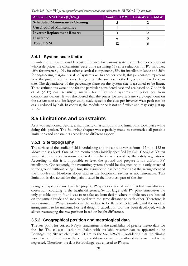
30
Table 3.9 Solar PV plant operation and maintenance cost estimates in EURO/kWp per year.
Annual O&M Costs (€/kWp) South, 1.1MW East-West, 6.6MW
Scheduled Maintenance/Cleaning 3 2
Unscheduled Maintenance 1 1
Inverter Replacement Reserve 3 2
Insurance 6 3
Total O&M 12 6
3.4.1. System scale factor
In order to illustrate possible cost difference for various system size due to component wholesale prices the calculations were done assuming 1% cost reduction for PV modules, 10% for inverters, 10% for other electrical components, 5% for installation labor and 30% for engineering margin in scale of system size. In another words, this percentages represent how the price of components change from the smallest to the largest considered system size. The dependence of the percentage share on the system size is assumed to be linear. These estimations were done for the particular considered case and are based on Goodrich et al. (2012) cost sensitivity analysis for utility scale systems and prices got from component dealers. It was discovered that the prices for inverters are very dependent on the system size and for larger utility scale systems the cost per inverter Watt peak can be easily reduced by half. In contrast, the module price is not so flexible and may vary just up to 5%.
3.5 Limitations and constraints
As it was mentioned before, a multiplicity of assumptions and limitations took place while doing this project. The following chapter was especially made to summarize all possible limitations and constraints according to different aspects.
3.5.1. Site topography
The surface of the studied field is undulating and the altitude varies from 117 m to 132 m above the sea level. One of the requirements initially specified by Falu Energi & Vatten was that none of excavations and soil disturbance is allowed by the safety regulations. According to this it is impossible to level the ground and prepare it for uniform PV installation. Consequently, the mounting system should be designed so it is only attached to the ground without piling. Thus, the assumption has been made that the arrangement of the modules on Northern slopes and in the bottom of ravines is not reasonable. This limitation is also actual for the plain located in the Northern part of the site. Being a major tool used in the project, PVsyst does not allow individual row distance correction according to the height difference. So for large scale PV plant simulation the only possible option found was to use flat uniform design where module rows are located on the same altitude and are arranged with the same distance to each other. Therefore, it was assumed in PVsyst simulations the surface to be flat and rectangular, and the module arrangement to be uniform. For real design a calculation tool has been developed, which allows rearranging the row position based on height difference.
3.5.2. Geographical position and metrological data
The key point for correct PVsyst simulations is the availability of precise meteo data for the site. The closest location to Falun with available weather data is appeared to be Borlänge, the city which situated 21 km to the South-West. Considering that the climate zone for both locations is the same, the difference in the weather data is assumed to be neglected. Therefore, the data for Borlänge was entered to PVsyst.
31
A significant limitation is the snow influence on system performance. In the design systems two different orientations were considered, South and East-West (EW) with tilts of 34° and 10° respectively. As for East-West solution this tilt is too low for free snow sliding, it is obvious that in this case the modules will be shaded and out of operation during longer time in the winter. So for a fair comparison in detailed design it was considered as necessary to make a correction for December, January and February, when the system with low tilt will be without operation a certain time. A rough estimation was done so that the EW system is covered with snow and out of operation 40% of available winter time.
3.5.3. Shadings
The shading effect on modules can be conditionally divided by three components: horizon shading, near shading and self-shading. Horizon shadings are caused by horizon line and far located objects. The best way to specify this component is to make horizon angle measurements and create a shading map in PVsyst. As the area of the field is quite large, the horizon shading profile differs slightly from place to place. Here a simplification was used and horizon shading pattern was assumed to be the same for all locations of the site. Small buildings surrounding the field were assumed to be a part of horizon component. Near shadings stand mainly for objects that are located close to solar installation. PVsyst allows creating a 3D model of the system and these objects and simulates the difference in shading profile during the sun movements. In this thesis project the near shading is considered to be created by buildings of a recycling plant, so these constructions were included in the 3D model used for detailed design. The assumption here was made for the buildings dimensions and precise locations in relation to the PV array, which were originally unknown. Finally, self-shading component describes the shading appearing in multiple row systems caused by a row standing front. In order to get precise results in PVsyst electrical shading effect option has been chosen for unlimited sheds profile used in preliminary sizing. For detailed design, where self-shading profile is set by the 3D model, 33% shading effect on electrical production has been chosen (default in PVsyst). This proportion was assumed to be realistic taking into account that a lot of diffuse radiation will affect the module performance because of the large between row distance.
3.5.4. Irradiation calculation method
While doing the optimization a substantial difference in results has been noticed depending on which anisotropic irradiation calculation model is used. PVsyst gives an opportunity to choose between Hay or Perez models. According to Duffie and Beckman (2013), Hay and Davies method is based on the assumption that all diffuse radiation can be represented by two parts, the isotropic and circumsolar. It estimates the circumsolar diffuse part of the radiation considered to be all from the same direction as the beam irradiation. The Perez et al. model is based on more detailed analysis and includes also horizon brightening. It is more complex and especially more sensitive to a realistic determination of diffuse irradiation. During pre-study by using preliminary section in PVsyst it was discovered that Hey model calculates the global irradiation on a tilted plane with 1158 kWh/m2 at optimal 43° tilt, while Perez method shows 1238 kWh/m2 at optimal 48°. It makes a difference of approximately 7%. However, this distinction might be even more crucial for low tilted plane simulations, which is especially important for EW solution. It also may lead to
32
significant mismatch in tilt optimization. Considering the fact that Perez model is more precise to diffuse radiation part, this method has been finally chosen as a default.
3.5.5. Electrical and mechanical layout
When it comes to electrical and mechanical layout, the system was simplified to a great extent because of two reasons. Firstly, as mentioned before the site is not flat, so it was considered the final module arrangement to be done during the construction process. Secondly, none of PV installation companies was willing to share the information about mounting details and costs. Consequently, the layout design is limited to module string sizing and numbering so that the array optimally fits to an inverter. Unfortunately, this leads to one more limitation, that cables length, connections, junction boxes and other related components cannot be properly designed as well as detailed mounting system design cannot be covered in the project. Therefore, approximate assumptions were done for mounting and cable costs.
3.5.6. Economical evaluation procedure
It is important to comment about limitations and constraints made in economical evaluation procedure, which assumption can affect the results to the greatest extend and may cause the major uncertainty part. The assumptions are following:
Quotes for Balance of System (BOS) costs presented in Tables 3.3, 3.4 and 3.9 are based on rough estimations and are approximate.
Engineering margin cost is assumed to be linearly dependent on system scale according to PV nominal power.
Quotes for electrical components (wires, connections, junction boxes, etc.) is assumed to be not affected by the between row distance difference.
Chosen inverters require special cabin to be installed in. The price of the cabin has not been included in calculation procedure.
The system requires power transformer to be connected to 10kV power grid. The transformer costs were not considered.
On a request of the company VAT tax and loans have not been included in the price.
4 Results and analysis This chapter contains the results of simulations, optimization and economical evaluation, which help to assess the project expediency with different options. The chapter is divided on two parts. Preliminary results describe the comparison of different components performance and optimization due to array orientation, tilt and row to row distance on example of a system with the same 100 kW inverter. The procedure of LCOE calculation for this part was simplified, which results cannot be considered as precise financial evaluation values as they do not include maintenance, permission and insurance. Nevertheless, it provides an opportunity to compare fairly different options and optimize the system. Eventually, the result of preliminary design represent two system options, considered by the author as worthwhile, which then were studied in detailed section. The detailed design results show the sizes, performance analysis and complex economical evaluation results of the two considered simulated options.
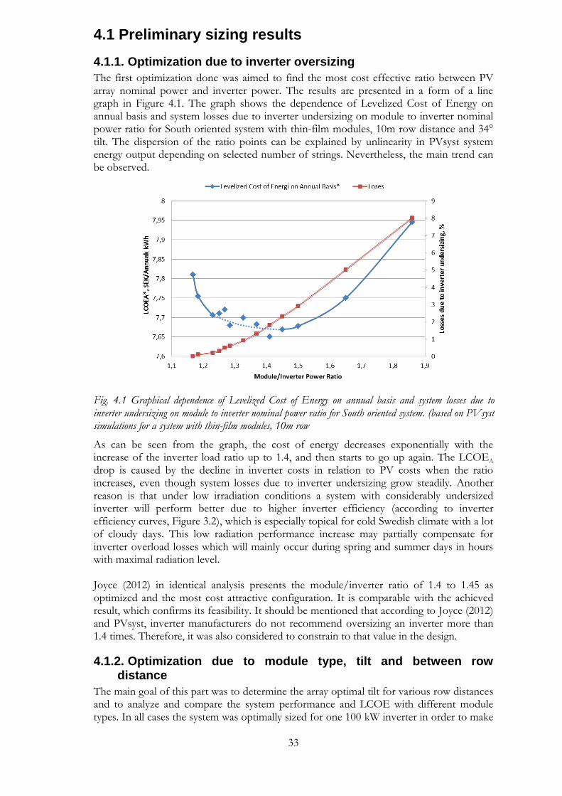
33
4.1 Preliminary sizing results
4.1.1. Optimization due to inverter oversizing
The first optimization done was aimed to find the most cost effective ratio between PV array nominal power and inverter power. The results are presented in a form of a line graph in Figure 4.1. The graph shows the dependence of Levelized Cost of Energy on annual basis and system losses due to inverter undersizing on module to inverter nominal power ratio for South oriented system with thin-film modules, 10m row distance and 34° tilt. The dispersion of the ratio points can be explained by unlinearity in PVsyst system energy output depending on selected number of strings. Nevertheless, the main trend can be observed.
As can be seen from the graph, the cost of energy decreases exponentially with the increase of the inverter load ratio up to 1.4, and then starts to go up again. The LCOEA drop is caused by the decline in inverter costs in relation to PV costs when the ratio increases, even though system losses due to inverter undersizing grow steadily. Another reason is that under low irradiation conditions a system with considerably undersized inverter will perform better due to higher inverter efficiency (according to inverter efficiency curves, Figure 3.2), which is especially topical for cold Swedish climate with a lot of cloudy days. This low radiation performance increase may partially compensate for inverter overload losses which will mainly occur during spring and summer days in hours with maximal radiation level. Joyce (2012) in identical analysis presents the module/inverter ratio of 1.4 to 1.45 as optimized and the most cost attractive configuration. It is comparable with the achieved result, which confirms its feasibility. It should be mentioned that according to Joyce (2012) and PVsyst, inverter manufacturers do not recommend oversizing an inverter more than 1.4 times. Therefore, it was also considered to constrain to that value in the design.
4.1.2. Optimization due to module type, tilt and between row distance
The main goal of this part was to determine the array optimal tilt for various row distances and to analyze and compare the system performance and LCOE with different module types. In all cases the system was optimally sized for one 100 kW inverter in order to make
Fig. 4.1 Graphical dependence of Levelized Cost of Energy on annual basis and system losses due to inverter undersizing on module to inverter nominal power ratio for South oriented system. (based on PVsyst simulations for a system with thin-film modules, 10m row
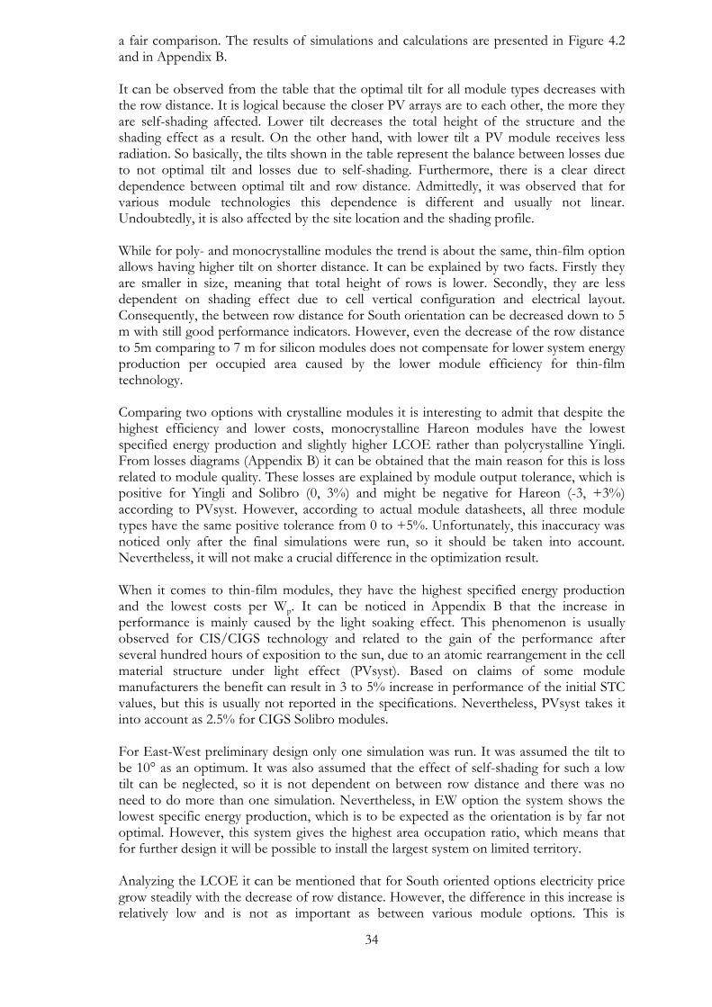
34
a fair comparison. The results of simulations and calculations are presented in Figure 4.2 and in Appendix B. It can be observed from the table that the optimal tilt for all module types decreases with the row distance. It is logical because the closer PV arrays are to each other, the more they are self-shading affected. Lower tilt decreases the total height of the structure and the shading effect as a result. On the other hand, with lower tilt a PV module receives less radiation. So basically, the tilts shown in the table represent the balance between losses due to not optimal tilt and losses due to self-shading. Furthermore, there is a clear direct dependence between optimal tilt and row distance. Admittedly, it was observed that for various module technologies this dependence is different and usually not linear. Undoubtedly, it is also affected by the site location and the shading profile. While for poly- and monocrystalline modules the trend is about the same, thin-film option allows having higher tilt on shorter distance. It can be explained by two facts. Firstly they are smaller in size, meaning that total height of rows is lower. Secondly, they are less dependent on shading effect due to cell vertical configuration and electrical layout. Consequently, the between row distance for South orientation can be decreased down to 5 m with still good performance indicators. However, even the decrease of the row distance to 5m comparing to 7 m for silicon modules does not compensate for lower system energy production per occupied area caused by the lower module efficiency for thin-film technology. Comparing two options with crystalline modules it is interesting to admit that despite the highest efficiency and lower costs, monocrystalline Hareon modules have the lowest specified energy production and slightly higher LCOE rather than polycrystalline Yingli. From losses diagrams (Appendix B) it can be obtained that the main reason for this is loss related to module quality. These losses are explained by module output tolerance, which is positive for Yingli and Solibro (0, 3%) and might be negative for Hareon (-3, +3%) according to PVsyst. However, according to actual module datasheets, all three module types have the same positive tolerance from 0 to +5%. Unfortunately, this inaccuracy was noticed only after the final simulations were run, so it should be taken into account. Nevertheless, it will not make a crucial difference in the optimization result. When it comes to thin-film modules, they have the highest specified energy production and the lowest costs per Wp. It can be noticed in Appendix B that the increase in performance is mainly caused by the light soaking effect. This phenomenon is usually observed for CIS/CIGS technology and related to the gain of the performance after several hundred hours of exposition to the sun, due to an atomic rearrangement in the cell material structure under light effect (PVsyst). Based on claims of some module manufacturers the benefit can result in 3 to 5% increase in performance of the initial STC values, but this is usually not reported in the specifications. Nevertheless, PVsyst takes it into account as 2.5% for CIGS Solibro modules. For East-West preliminary design only one simulation was run. It was assumed the tilt to be 10° as an optimum. It was also assumed that the effect of self-shading for such a low tilt can be neglected, so it is not dependent on between row distance and there was no need to do more than one simulation. Nevertheless, in EW option the system shows the lowest specific energy production, which is to be expected as the orientation is by far not optimal. However, this system gives the highest area occupation ratio, which means that for further design it will be possible to install the largest system on limited territory. Analyzing the LCOE it can be mentioned that for South oriented options electricity price grow steadily with the decrease of row distance. However, the difference in this increase is relatively low and is not as important as between various module options. This is
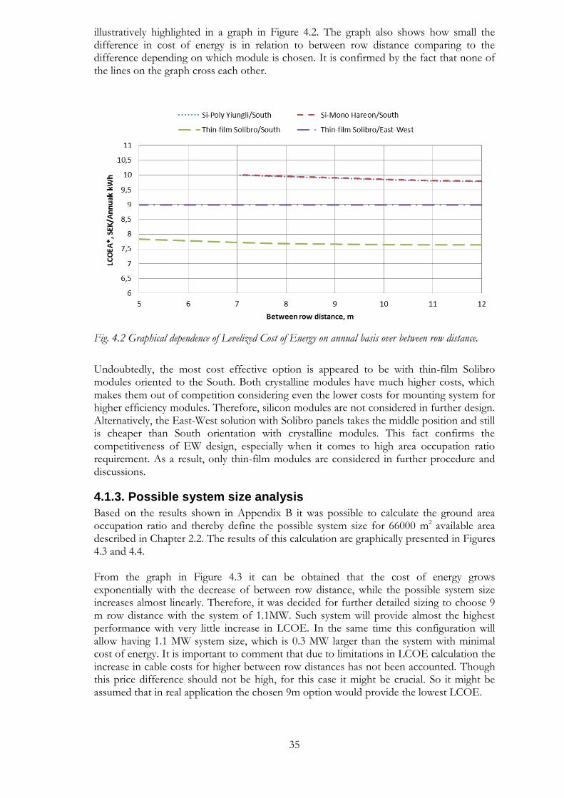
35
illustratively highlighted in a graph in Figure 4.2. The graph also shows how small the difference in cost of energy is in relation to between row distance comparing to the difference depending on which module is chosen. It is confirmed by the fact that none of the lines on the graph cross each other.
Fig. 4.2 Graphical dependence of Levelized Cost of Energy on annual basis over between row distance.
Undoubtedly, the most cost effective option is appeared to be with thin-film Solibro modules oriented to the South. Both crystalline modules have much higher costs, which makes them out of competition considering even the lower costs for mounting system for higher efficiency modules. Therefore, silicon modules are not considered in further design. Alternatively, the East-West solution with Solibro panels takes the middle position and still is cheaper than South orientation with crystalline modules. This fact confirms the competitiveness of EW design, especially when it comes to high area occupation ratio requirement. As a result, only thin-film modules are considered in further procedure and discussions.
4.1.3. Possible system size analysis
Based on the results shown in Appendix B it was possible to calculate the ground area occupation ratio and thereby define the possible system size for 66000 m2 available area described in Chapter 2.2. The results of this calculation are graphically presented in Figures 4.3 and 4.4. From the graph in Figure 4.3 it can be obtained that the cost of energy grows exponentially with the decrease of between row distance, while the possible system size increases almost linearly. Therefore, it was decided for further detailed sizing to choose 9 m row distance with the system of 1.1MW. Such system will provide almost the highest performance with very little increase in LCOE. In the same time this configuration will allow having 1.1 MW system size, which is 0.3 MW larger than the system with minimal cost of energy. It is important to comment that due to limitations in LCOE calculation the increase in cable costs for higher between row distances has not been accounted. Though this price difference should not be high, for this case it might be crucial. So it might be assumed that in real application the chosen 9m option would provide the lowest LCOE.
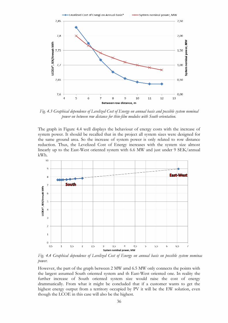
36
Fig. 4.3 Graphical dependence of Levelized Cost of Energy on annual basis and possible system nominal
power on between row distance for thin-film modules with South orientation.
The graph in Figure 4.4 well displays the behaviour of energy costs with the increase of system power. It should be recalled that in the project all system sizes were designed for the same ground area. So the increase of system power is only related to row distance reduction. Thus, the Levelized Cost of Energy increases with the system size almost linearly up to the East-West oriented system with 6.6 MW and just under 9 SEK/annual kWh.
However, the part of the graph between 2 MW amd 6.5 MW only connects the points with the largest assumed South oriented system and th East-West oriented one. In reality the further increase of South oriented system size would raise the cost of energy drammatically. From what it might be concluded that if a customer wants to get the highest energy output from a territory occupied by PV it will be the EW solution, even though the LCOE in this case will also be the highest.
Fig. 4.4 Graphical dependence of Levelized Cost of Energy on annual basis on possible system nominal power.
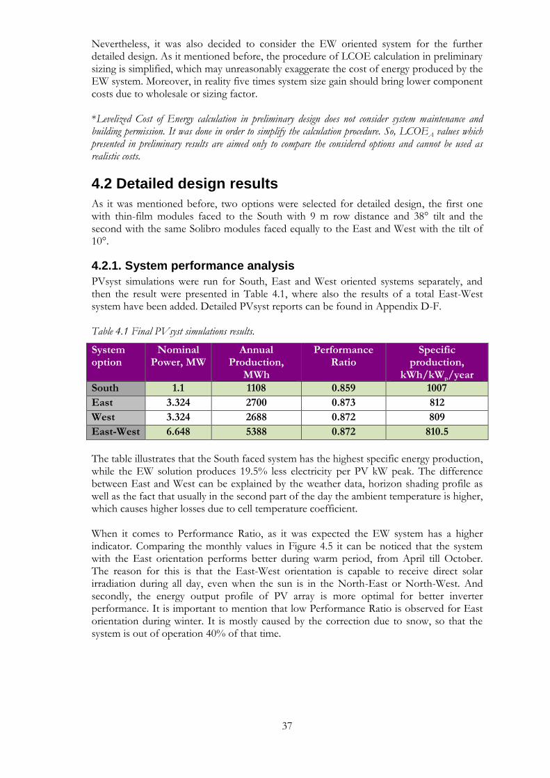
37
Nevertheless, it was also decided to consider the EW oriented system for the further detailed design. As it mentioned before, the procedure of LCOE calculation in preliminary sizing is simplified, which may unreasonably exaggerate the cost of energy produced by the EW system. Moreover, in reality five times system size gain should bring lower component costs due to wholesale or sizing factor. *Levelized Cost of Energy calculation in preliminary design does not consider system maintenance and building permission. It was done in order to simplify the calculation procedure. So, LCOEA values which presented in preliminary results are aimed only to compare the considered options and cannot be used as realistic costs.
4.2 Detailed design results
As it was mentioned before, two options were selected for detailed design, the first one with thin-film modules faced to the South with 9 m row distance and 38° tilt and the second with the same Solibro modules faced equally to the East and West with the tilt of 10°.
4.2.1. System performance analysis
PVsyst simulations were run for South, East and West oriented systems separately, and then the result were presented in Table 4.1, where also the results of a total East-West system have been added. Detailed PVsyst reports can be found in Appendix D-F. Table 4.1 Final PVsyst simulations results.
System option
Nominal Power, MW
Annual Production,
MWh
Performance Ratio
Specific production,
kWh/kWp/year
South 1.1 1108 0.859 1007
East 3.324 2700 0.873 812
West 3.324 2688 0.872 809
East-West 6.648 5388 0.872 810.5
The table illustrates that the South faced system has the highest specific energy production, while the EW solution produces 19.5% less electricity per PV kW peak. The difference between East and West can be explained by the weather data, horizon shading profile as well as the fact that usually in the second part of the day the ambient temperature is higher, which causes higher losses due to cell temperature coefficient. When it comes to Performance Ratio, as it was expected the EW system has a higher indicator. Comparing the monthly values in Figure 4.5 it can be noticed that the system with the East orientation performs better during warm period, from April till October. The reason for this is that the East-West orientation is capable to receive direct solar irradiation during all day, even when the sun is in the North-East or North-West. And secondly, the energy output profile of PV array is more optimal for better inverter performance. It is important to mention that low Performance Ratio is observed for East orientation during winter. It is mostly caused by the correction due to snow, so that the system is out of operation 40% of that time.
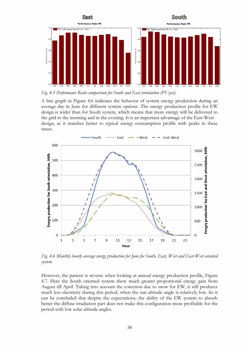
38
Fig. 4.5 Performance Ratio comparison for South and East orientation (PVsyst).
A line graph in Figure 4.6 indicates the behavior of system energy production during an average day in June for different system options. The energy production profile for EW design is wider than for South system, which means that more energy will be delivered to the grid in the morning and in the evening. It is an important advantage of the East-West design, as it matches better to typical energy consumption profile with peaks in these times.
Fig. 4.6 Monthly hourly average energy production for June for South, East, West and East-West oriented system.
However, the pattern is reverse when looking at annual energy production profile, Figure 4.7. Here the South oriented system show much greater proportional energy gain from August till April. Taking into account the corection due to snow for EW, it still produces much less electricity during this period, when the sun altitude angle is relatively low. So it can be concluded that despite the expectations, the ability of the EW system to absorb better the diffuse irradiation part does not make this configuration more profitable for the period with low solar altitude angles.
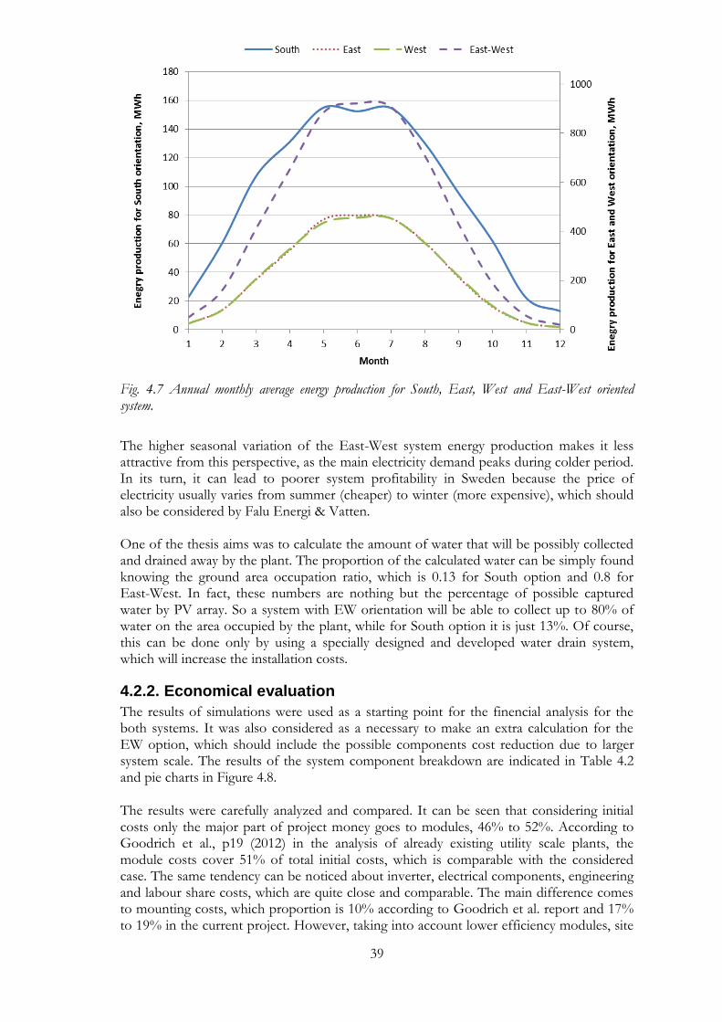
39
Fig. 4.7 Annual monthly average energy production for South, East, West and East-West oriented system.
The higher seasonal variation of the East-West system energy production makes it less attractive from this perspective, as the main electricity demand peaks during colder period. In its turn, it can lead to poorer system profitability in Sweden because the price of electricity usually varies from summer (cheaper) to winter (more expensive), which should also be considered by Falu Energi & Vatten. One of the thesis aims was to calculate the amount of water that will be possibly collected and drained away by the plant. The proportion of the calculated water can be simply found knowing the ground area occupation ratio, which is 0.13 for South option and 0.8 for East-West. In fact, these numbers are nothing but the percentage of possible captured water by PV array. So a system with EW orientation will be able to collect up to 80% of water on the area occupied by the plant, while for South option it is just 13%. Of course, this can be done only by using a specially designed and developed water drain system, which will increase the installation costs.
4.2.2. Economical evaluation
The results of simulations were used as a starting point for the finencial analysis for the both systems. It was also considered as a necessary to make an extra calculation for the EW option, which should include the possible components cost reduction due to larger system scale. The results of the system component breakdown are indicated in Table 4.2 and pie charts in Figure 4.8.
The results were carefully analyzed and compared. It can be seen that considering initial costs only the major part of project money goes to modules, 46% to 52%. According to Goodrich et al., p19 (2012) in the analysis of already existing utility scale plants, the module costs cover 51% of total initial costs, which is comparable with the considered case. The same tendency can be noticed about inverter, electrical components, engineering and labour share costs, which are quite close and comparable. The main difference comes to mounting costs, which proportion is 10% according to Goodrich et al. report and 17% to 19% in the current project. However, taking into account lower efficiency modules, site

40
special requirements and land safety regulations it is reasonable to assume the higher costs for mounting as realistic because the installation will require not only special individual adjustment according to the ground relief but also a special racking system, which will be attached to the ground and weighted with concrete blocks. Nevertheless, it was not possible to cover the mounting detailed design in this thesis, so these costs can be only based on assumptions. Therefore, in more careful study it might be discovered the lower costs for mounting share.
Table 4.2 Final pricing of the proposed 1.1 MW South oriented system, 6.65 MW East-West oriented system and the same East-West system including possible cost reduction due to system scale.
Components/Costs in EURO South East-West East-West Including scale factor
Modules 473 000 2 858 640 2 830 054
Inverters 76 758 383 790 345 411
Mounting 198 000 930 720 930 720
Electrical 74 776 417 315 375 584
Installation labour 123 380 688 570 654 141
Shipping 16 451 91 809 89 635
Engineering 41 127 229 523 160 666
Permission 11 000 11 000 11 000
Initial cost 833 534 4 601 465 4 492 768
Annual insurance 6600 19800 19800
Annual maintenance 14 300 46 536 46 536
Total maintenance over 25 years 522 500 1 658 400 1 658 400
Fig. 4.8 Costs breakdown for South oriented 1.1 MW system (to the left) and for East-West 6.65 MW system with possible cost reduction due to system scale (to the right). Two diagrams on the top represent total project costs including operation and maintenance costs over 25 years lifetime period. The pie charts on the bottom show breakdowns for initial costs only (excluding maintenance).
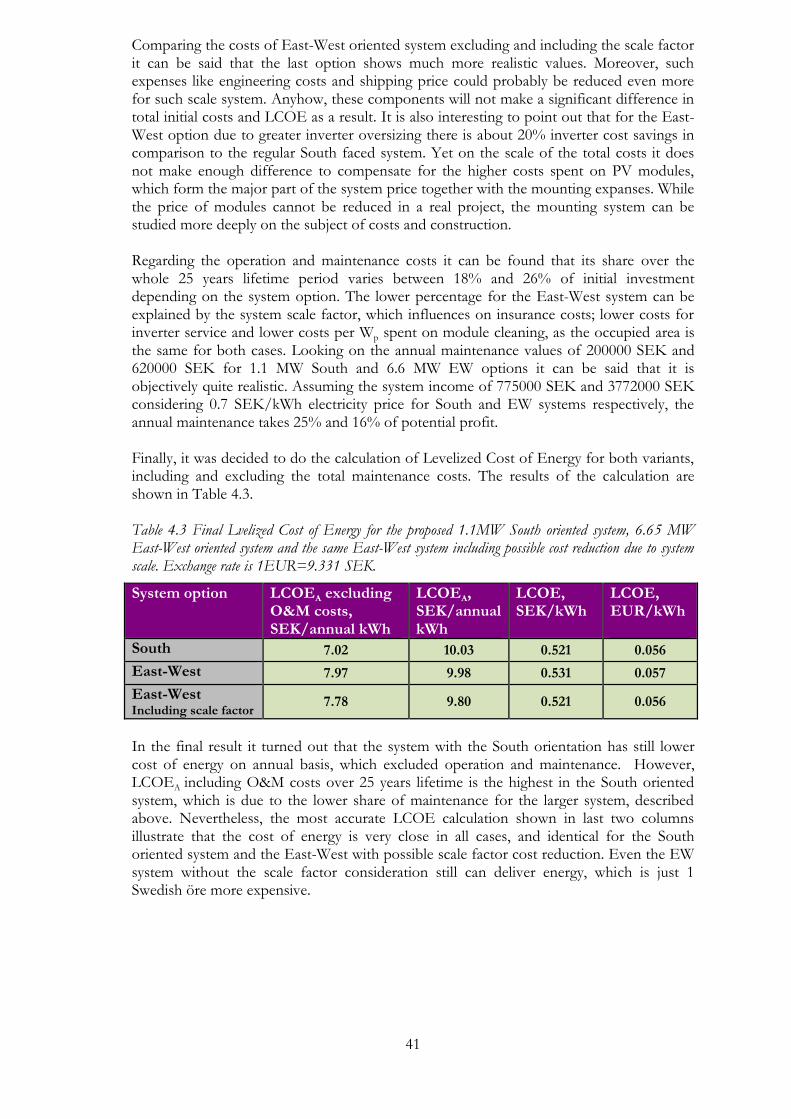
41
Comparing the costs of East-West oriented system excluding and including the scale factor it can be said that the last option shows much more realistic values. Moreover, such expenses like engineering costs and shipping price could probably be reduced even more for such scale system. Anyhow, these components will not make a significant difference in total initial costs and LCOE as a result. It is also interesting to point out that for the East-West option due to greater inverter oversizing there is about 20% inverter cost savings in comparison to the regular South faced system. Yet on the scale of the total costs it does not make enough difference to compensate for the higher costs spent on PV modules, which form the major part of the system price together with the mounting expanses. While the price of modules cannot be reduced in a real project, the mounting system can be studied more deeply on the subject of costs and construction. Regarding the operation and maintenance costs it can be found that its share over the whole 25 years lifetime period varies between 18% and 26% of initial investment depending on the system option. The lower percentage for the East-West system can be explained by the system scale factor, which influences on insurance costs; lower costs for inverter service and lower costs per Wp spent on module cleaning, as the occupied area is the same for both cases. Looking on the annual maintenance values of 200000 SEK and 620000 SEK for 1.1 MW South and 6.6 MW EW options it can be said that it is objectively quite realistic. Assuming the system income of 775000 SEK and 3772000 SEK considering 0.7 SEK/kWh electricity price for South and EW systems respectively, the annual maintenance takes 25% and 16% of potential profit. Finally, it was decided to do the calculation of Levelized Cost of Energy for both variants, including and excluding the total maintenance costs. The results of the calculation are shown in Table 4.3. Table 4.3 Final Lvelized Cost of Energy for the proposed 1.1MW South oriented system, 6.65 MW East-West oriented system and the same East-West system including possible cost reduction due to system scale. Exchange rate is 1EUR=9.331 SEK.
System option LCOEA excluding O&M costs, SEK/annual kWh
LCOEA, SEK/annual kWh
LCOE, SEK/kWh
LCOE, EUR/kWh
South 7.02 10.03 0.521 0.056
East-West 7.97 9.98 0.531 0.057
East-West Including scale factor
7.78 9.80 0.521 0.056
In the final result it turned out that the system with the South orientation has still lower cost of energy on annual basis, which excluded operation and maintenance. However, LCOEA including O&M costs over 25 years lifetime is the highest in the South oriented system, which is due to the lower share of maintenance for the larger system, described above. Nevertheless, the most accurate LCOE calculation shown in last two columns illustrate that the cost of energy is very close in all cases, and identical for the South oriented system and the East-West with possible scale factor cost reduction. Even the EW system without the scale factor consideration still can deliver energy, which is just 1 Swedish öre more expensive.
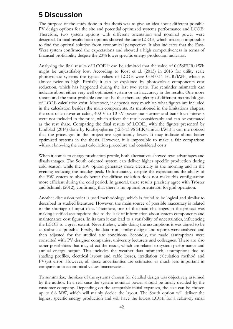
42
5 Discussion The purpose of the study done in this thesis was to give an idea about different possible PV design options for the site and potential optimized systems performance and LCOE. Therefore, two system options with different orientation and nominal power were designed. In final results both options showed the same LCOE, which makes it impossible to find the optimal solution from economical perspective. It also indicates that the East-West system confirmed the expectations and showed a high competitiveness in terms of financial profitability despite the 20% lower specific energy production indicator. Analyzing the final results of LCOE it can be admitted that the value of 0.056EUR/kWh might be unjustifiably low. According to Kost et al. (2013) in 2013 for utility scale photovoltaic systems the typical values of LCOE were 0.08-0.11 EUR/kWh, which is almost twice as high. Partially it can be explained by photovoltaic components cost reduction, which has happened during the last two years. The reminder mismatch can indicate about either very well optimized system or an inaccuracy in the results. One more reason and the most probable one can be that there are plenty of different methodologies of LCOE calculation exist. Moreover, it depends very much on what figures are included in the calculation besides the main components. As mentioned in the limitations chapter, the cost of an inverter cabin, 400 V to 10 kV power transformer and bank loan interests were not included in the price, which affects the result considerably and can be estimated as the rest share. Comparing the final results of LCOEA with the figures presented by Lindblad (2014) done by Kraftspojkarna (12.6-13.96 SEK/annual kWh) it can me noticed that the prices got in the project are significantly lower. It may indicate about better optimized systems in the thesis. However, it is impossible to make a fair comparison without knowing the exact calculation procedure and considered costs. When it comes to energy production profile, both alternatives showed own advantages and disadvantages. The South oriented system can deliver higher specific production during cold season, while the EW option generates more electricity in the morning and in the evening reducing the midday peak. Unfortunately, despite the expectations the ability of the EW system to absorb better the diffuse radiation does not make this configuration more efficient during the cold period. In general, these results precisely agree with Tröster and Schmidt (2012), confirming that there is no optimal orientation for grid operation. Another discussion point is used methodology, which is found to be logical and similar to described in studied literature. However, the main source of possible inaccuracy is related to the shortage of input data. Therefore, one of the main challenges in the project was making justified assumptions due to the lack of information about system components and maintenance cost figures. In its turn it can lead to a variability of uncertainties, influencing the LCOE to a great extent. Nevertheless, while doing the assumptions it was aimed to be as realistic as possible. Firstly, the data from similar designs and reports were analyzed and then adjusted for the studied site conditions. Secondly, the made assumptions were consulted with PV designer companies, university lecturers and colleagues. There are also other possibilities that may affect the result, which are related to system performance and annual energy output. This includes the weather data mismatch, assumptions due to shading profiles, electrical layout and cable losses, irradiation calculation method and PVsyst error. However, all these uncertainties are estimated as much less important in comparison to economical values inaccuracies. To summarize, the sizes of the systems chosen for detailed design was objectively assumed by the author. In a real case the system nominal power should be finally decided by the customer company. Depending on the acceptable initial expanses, the size can be chosen up to 6.6 MW, which will mainly decide the layout. The South option will deliver the highest specific energy production and will have the lowest LCOE for a relatively small
43
system up to 1MW. The advantage of the East-West orientation is the highest ground area occupation ratio, meaning that it allows installing the largest PV system on a limited space. Moreover, the EW is a new concept of PV design, which can lead to better advertising effect. In addition, it allows covering up to 80% of an occupied area and collecting corresponding proportion of rain water. Finally, considering the specific area configuration for the site it is also possible to suggest a combination of both orientations for the project. Such solution would fit better to the available area dimensions and might be a good object for doing a comparative research.
6 Conclusion In general it is possible to say that the aims of the study were successfully fulfilled. It was presented two system alternatives, which cover the same area assumed to be suitable for PV installation. The systems have completely diverse design and size, 1.1 MW for South
and 6.6 MW for East-West orientation; and therefore the initial investment of 835,000€
and 4500,000 € respectively. Both systems were optimized based on components profitability and configuration performance. Consequently, in final results both systems showed the same LCOE of 0.056 €/kWh, which is rather competitive comparing to other utility scale plants. It means that the East-West option demonstrated a high competitiveness in terms of financial profitability despite the 20% lower specific energy production. The main benefit is gained by the component cost reduction due to sizing factor and lower price of inverters, mounting and annual maintenance. When it comes to electricity production profile, it turned out that there is no optimal orientation and every PV setup has its pros and cons. The East-West system has better daily profile with lower midday peak and higher performance in mornings and evenings. On the other hand, the South option gains relatively more energy during cold seasons, when the demand is higher and the electricity in Sweden is more expensive. The expectations for EW solution to offset by higher performance with diffuse radiation during winter time were not met. However, for the case the EW system can have a considerable privilege. As the studied territory is highly contaminated, it can allow collecting up to 80% of rain water on the area occupied by the plant. South orientation can collect just 13% in contrast. Additionally, the East-West is a relatively new concept of PV design, which can result in better advertising effect for the project and will be a good subject for further research and development. A plenty of limitations and assumptions were made in the thesis. The main source of potential uncertainties might be caused by assumptions for BOS component costs, mounting costs and expenses for plant operation and maintenance, which were made due to the lack of information and time shortage. Nevertheless, the work should be considered as a base, allowing to evaluate the prospective project rationality. Though, if the proposition goes further, much more detailed design will have to be done. It should include detailed study and the design of module mounting system, mechanical and electrical system layout and component connection on both AC and DC sides, and monitoring equipment involvement. From economical perspective BOS, mounting and maintenance costs could be carefully studied being the main source of a possible inaccuracy.
44
References
APPLEYARD, D. (2000) Photovoltaics for northern latitudes. Modern Power Systems, Oct2000, Vol. 20 Issue 10, p59 BONFIGLIO, A. et al. (2014) Criteria for the Equivalent Modeling of Large Photovoltaic Power Plants. IEEE BRECL, K. & TOPIC, M. (2011) Self-shading losses of fixed free-standing PV arrays. Renewable Energy 36 3211-3216 CAMBELL, M. (2008) The drivers of the Levelized Cost of Electricity for utility-scale photovoltaics. Sunpower Corporation. San Jose, CA, USA DARLING, S.B. YOU, F. & VESELKA, T. (n.d.) Assumptions and the Levelized Cost of Energy for Photovoltaics. Available from: http://www.mcs.anl.gov/papers/P1810.pdf [Accessed 15.05.15] DUFFIE, J. & BECKMAN, W. (2013) Solar Engineering of Thermal Processes, 4th edition, John Wiley and Sons, p89-94 EEHD (2015) Photovoltaic trading company. Available from: http://www.eehd.de/angebote [Accessed 3.05.15] ELERCHIMAN.R (2013) Utilizing string inverters in large commercial systems. Available from: http://sunlightelectric.com/pdf/SP6.5_FE_Erlichman_v5.pdf [Accessed 11.05.15] FALU ENERGI & VATTEN (2015) Personal communication with the company. Available from: http://www.fev.se/privat/ [Accessed 03.06.15] FRONIUS (2011) Efficient east-west orientated PV systems with one MPP tracker. Available from: http://www.fronius.com/cps/rde/xbcr/SID-AF30EAED-B3F2642E/fronius_international/SE_TEA_Efficient_East_West_orientated_PV_systems_with_MPP_tracker_EN_357684_snapshot.pdf [Accessed 21.04.15] GOODRICH, A. JAMES, T. & WOODHOUSE, M. (2012) Residential, Commercial, and Utility-Scale Photovoltaic (PV) System Prices in the United States: Current Drivers and Cost-Reduction Opportunities. Oak Ridge, USA. NREL/TP-6A20-5334 HAYNES, T. (2013) Master thesis: Design and assessment of a large photovoltaic system in Barbados. Borlange, Sweden. ESES HERNANDEZ, V.M. (2012) Master thesis: Performance Evaluation of Different PV-Array Configurations under Weak Light Conditions and Partial Shadings. Borlänge, Sweden. ESES JACOBI, J. & STARKWEATHER, R. (2010) Solar Photovoltaic Plant Operating and Maintenance Costs. Available from: http://www.scottmadden.com/insight/407/solar-photovoltaic-plant-operating-and-maintenance-costs.html [Accessed 20.05.15] JORDAN, C.D. & KURTZ S.R. (2012) Photovoltaic Degradation Rates. Oak Ridge, USA. NREL/JA-5200-51664
45
JOYCE, K. (2012) Optimizing PV Plant Design to Achieve a Low Levelized Cost of Energy. Black & Veatch. Power-Gen International KEREKES, T. et al. (2013) An Optimization Method for Designing Large PV Plants. IEEE Journal of Photovoltaics, vol. 3, no. 2, April 2013 KOST, C. et al. (2013) Levelized Cost of Electricity Renewable Energy Technologies. p2 LINDBLAD, A. (2014) Project Report: Förstudie Solkraftverk på Syrafabriksområdet, Falun. Kraftpojkarna AB LÄNSSTYRELSEN DALARNA, MILJÖVÅRDSENHETEN. (2002) Falu Gruva Och Tillhörande Industrier . Available from: http://www.lansstyrelsen.se/dalarna/SiteCollectionDocuments/Sv/Publikationer/Rapporter-2002/02-12.pdf [Accessed 14.04.15] MACKNICK, J. et al. (2013) Solar Development on Contaminated and Disturbed Lands. Denver, USA, NREL/TP-6A20-58485 MECK, R. Calculating Tilted Array Spacing. Affordable Solar. Available from: http://www.affordable-solar.com/Learning-Center/Building-a-System/Calculating-Tilted-Array-Spacing [Accessed 27.04.15] METEONORM (2015) Metrological software. Available from: http://meteonorm.com/ [Accessed 22.04.15] NOAA Solar calculator (2015) Available from: http://www.esrl.noaa.gov/gmd/grad/solcalc/ [Accessed 11.05.15] PVSHOP (2015) PhotoVoltaic Solar Systems. Available from: http://pvshop.eu/power-one [Accessed 10.05.15] PVSYST V6.3.7. (2015) Photovoltaic software. Available from: http://www.pvsyst.com/en/ [Accessed 11.05.15] RENUSOL (2014) Increased solar output with the Renusol East-West system. Available from: http://www.renusol.com/en/company/news/news-imgvid/article/973.html [Accessed 21.04.15] SANCHEZ REINOSO, C.R. DE PAULA, M. & BUITRAGO R.H. Cost-benefit analysis of a photovoltaic power plant. International journal of hydrogen energy 39 (2014) 8708-8711 SANKAR, A. & KALATHIL, A. (2014) Qualitative validation of empirically observed higher generation in East-West oriented PV arrays over conventional South orientation. IEEE 978-1-4799-7606 SOLIBRO (2015) Photovoltaic module manufacturer. Personal communication with the company managers. Available from: http://solibro-solar.com/en/home/ Accessed [04.05.15] TRAPANI, K. & SANTAFÉ M.R. (2013) Project Report: A review of floating photovoltaic installations: 2007–2013 TRITEC (2015) Photovoltaic trading company. Available from: http://www.tritec-energy.com/en/products-overview/solar-modules-c-6/ [Accessed 04.05.15]
46
TRÖSTER, E. & SCHMIDT, J. (2012) Evaluating the impact of PV module orientation on grid operation. Available from: http://www.smooth-pv.info/doc/App22_ENA_Evaluating_the_Impact_of_PV_Module_Orientation.pdf [Accessed 28.05.15] VELOSA, A. & ABOUDI, M. (2014) What Is Inside Your LCOE Assumptions? Available from: http://mercomcapital.com/what-is-inside-your-lcoe-assumptions [Accessed 11.05.15] WIKIMAPIA maps. Available from: http://wikimapia.org/#lang=en&lat=60.610985&lon=15.613890&z=16&m=b [Accessed 24.05.15]

47
Appendix A: Component Specification Sheets
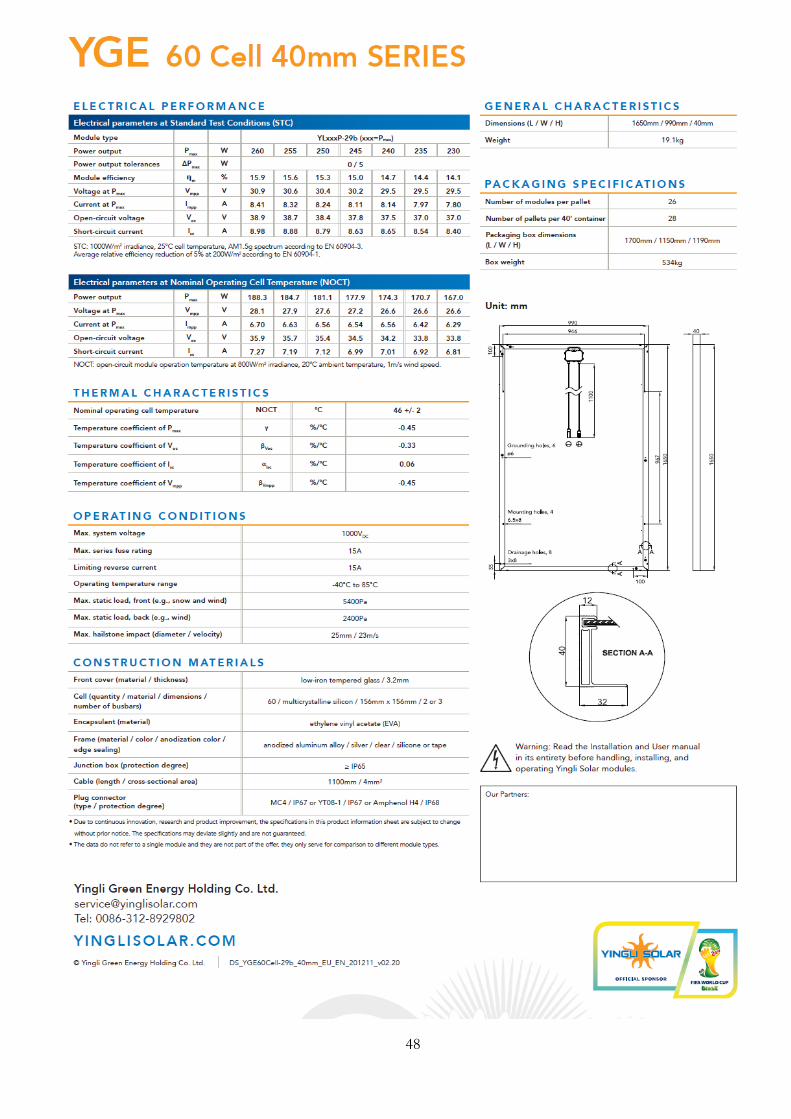
48
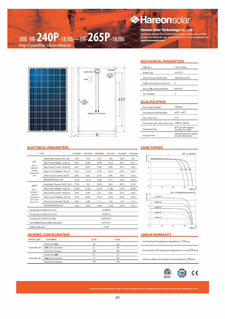
49
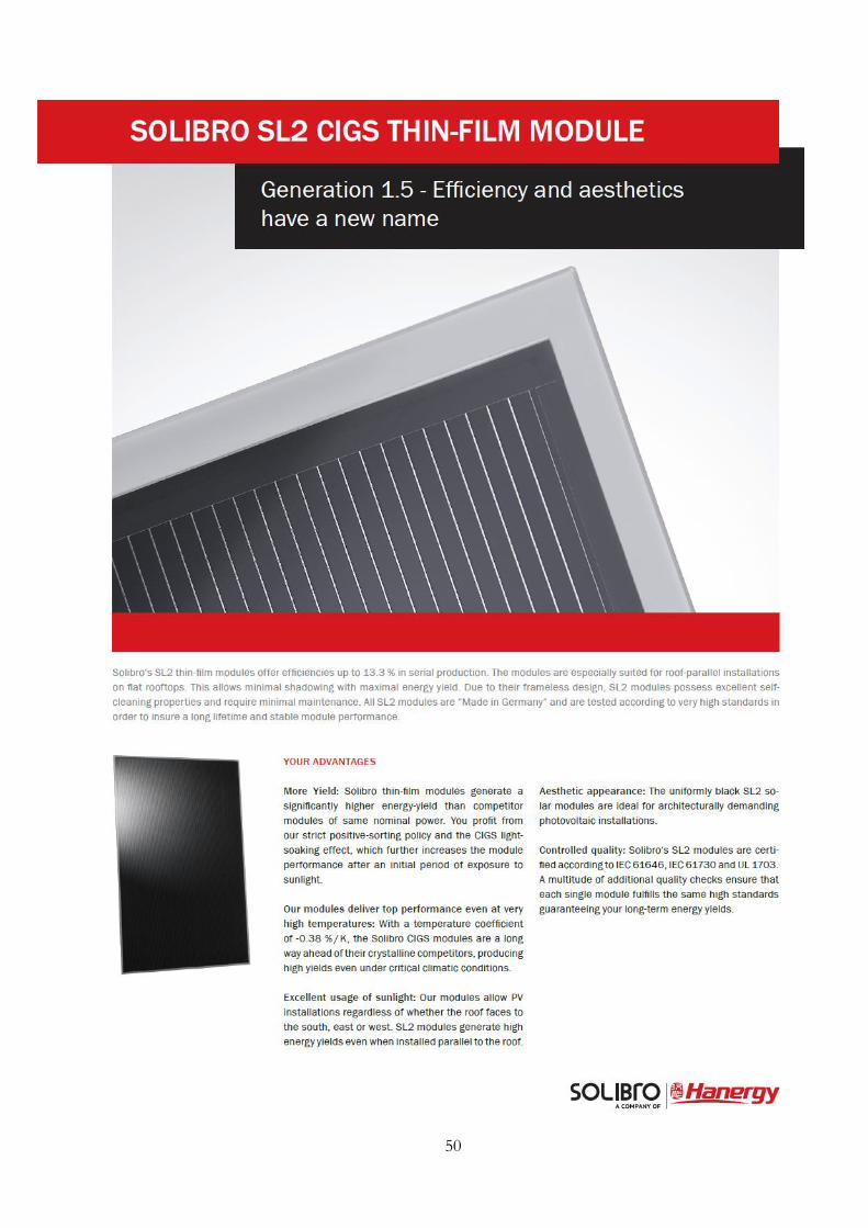
50
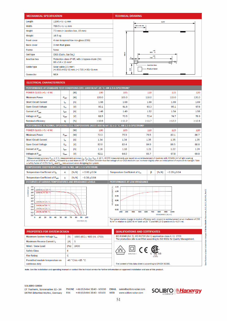
51
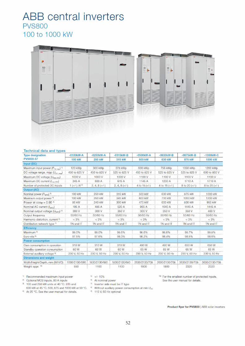
52
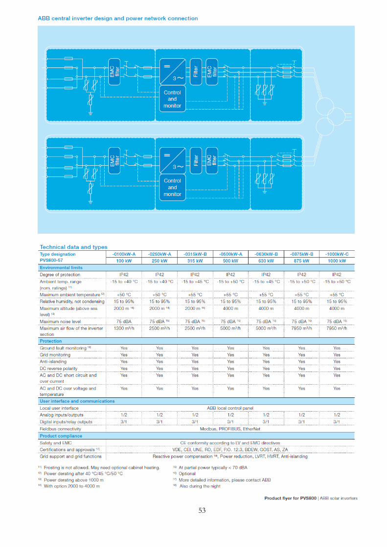
53
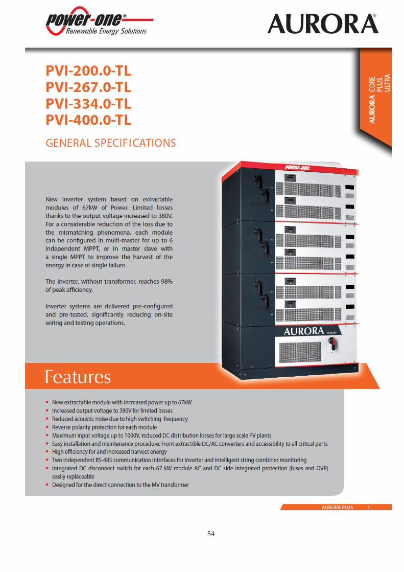
54
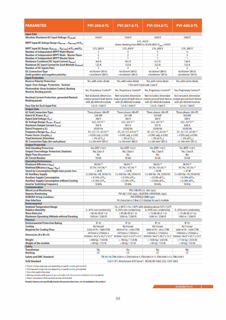
55
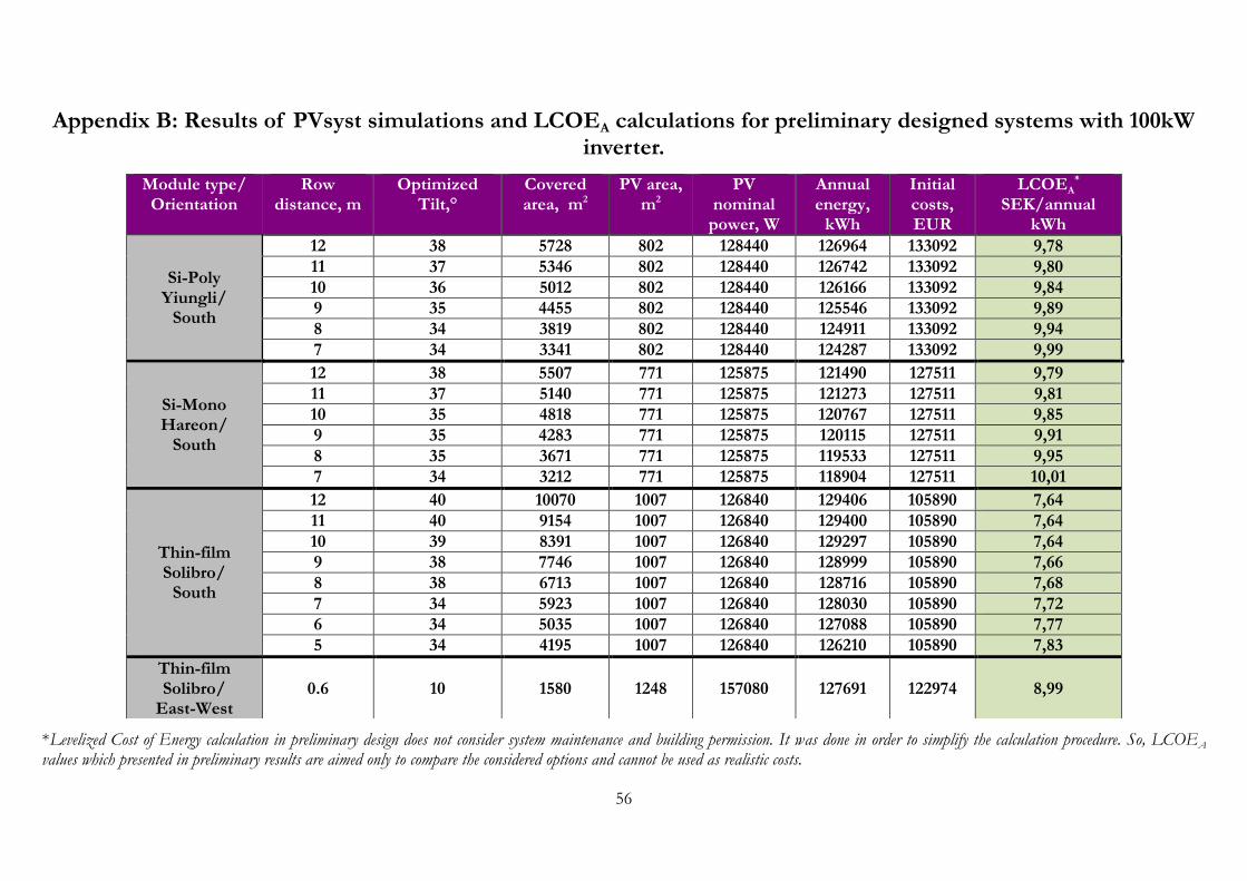
56
Appendix B: Results of PVsyst simulations and LCOEA calculations for preliminary designed systems with 100kW inverter.
*Levelized Cost of Energy calculation in preliminary design does not consider system maintenance and building permission. It was done in order to simplify the calculation procedure. So, LCOEA values which presented in preliminary results are aimed only to compare the considered options and cannot be used as realistic costs.
Module type/ Orientation
Row distance, m
Optimized Tilt,°
Covered area, m2
PV area, m2
PV nominal
power, W
Annual energy,
kWh
Initial costs, EUR
LCOEA*
SEK/annual kWh
Si-Poly
Yiungli/ South
12 38 5728 802 128440 126964 133092 9,78
11 37 5346 802 128440 126742 133092 9,80
10 36 5012 802 128440 126166 133092 9,84
9 35 4455 802 128440 125546 133092 9,89
8 34 3819 802 128440 124911 133092 9,94
7 34 3341 802 128440 124287 133092 9,99
Si-Mono Hareon/
South
12 38 5507 771 125875 121490 127511 9,79
11 37 5140 771 125875 121273 127511 9,81
10 35 4818 771 125875 120767 127511 9,85
9 35 4283 771 125875 120115 127511 9,91
8 35 3671 771 125875 119533 127511 9,95
7 34 3212 771 125875 118904 127511 10,01
Thin-film Solibro/
South
12 40 10070 1007 126840 129406 105890 7,64
11 40 9154 1007 126840 129400 105890 7,64
10 39 8391 1007 126840 129297 105890 7,64
9 38 7746 1007 126840 128999 105890 7,66
8 38 6713 1007 126840 128716 105890 7,68
7 34 5923 1007 126840 128030 105890 7,72
6 34 5035 1007 126840 127088 105890 7,77
5 34 4195 1007 126840 126210 105890 7,83
Thin-film Solibro/
East-West 0.6 10 1580 1248 157080 127691 122974 8,99
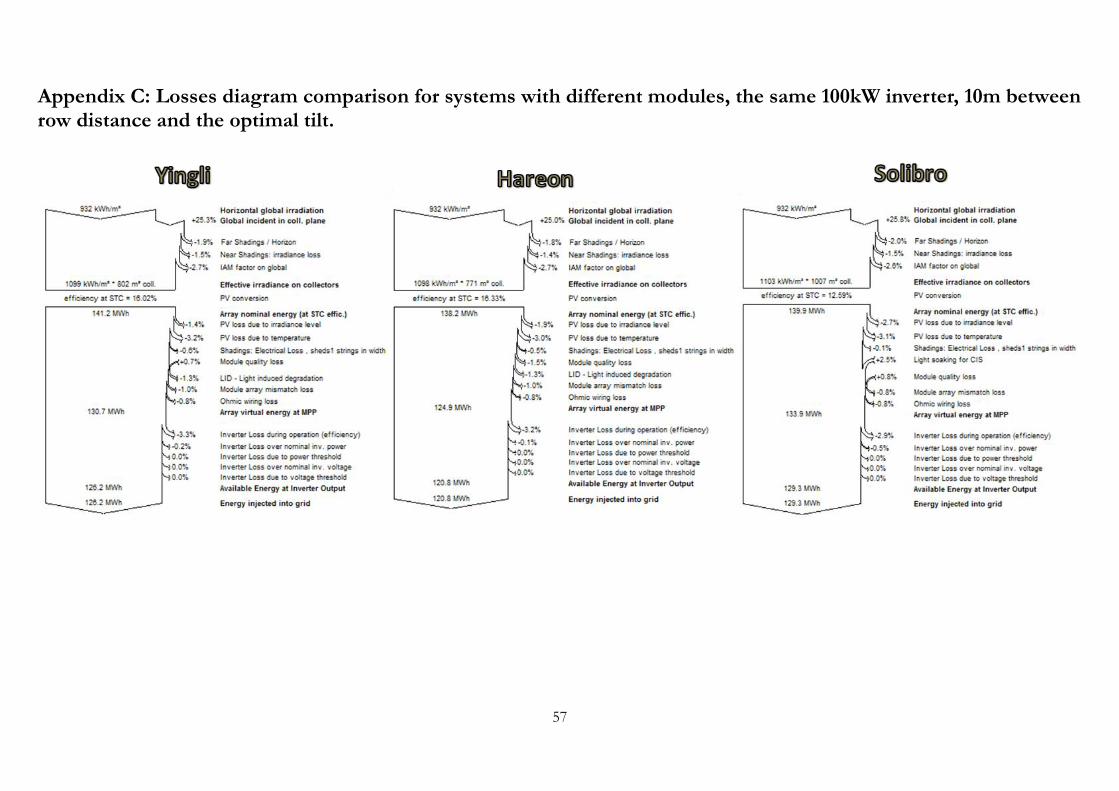
57
Appendix C: Losses diagram comparison for systems with different modules, the same 100kW inverter, 10m between row distance and the optimal tilt.
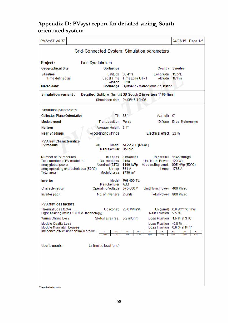
58
Appendix D: PVsyst report for detailed sizing, South orientated system
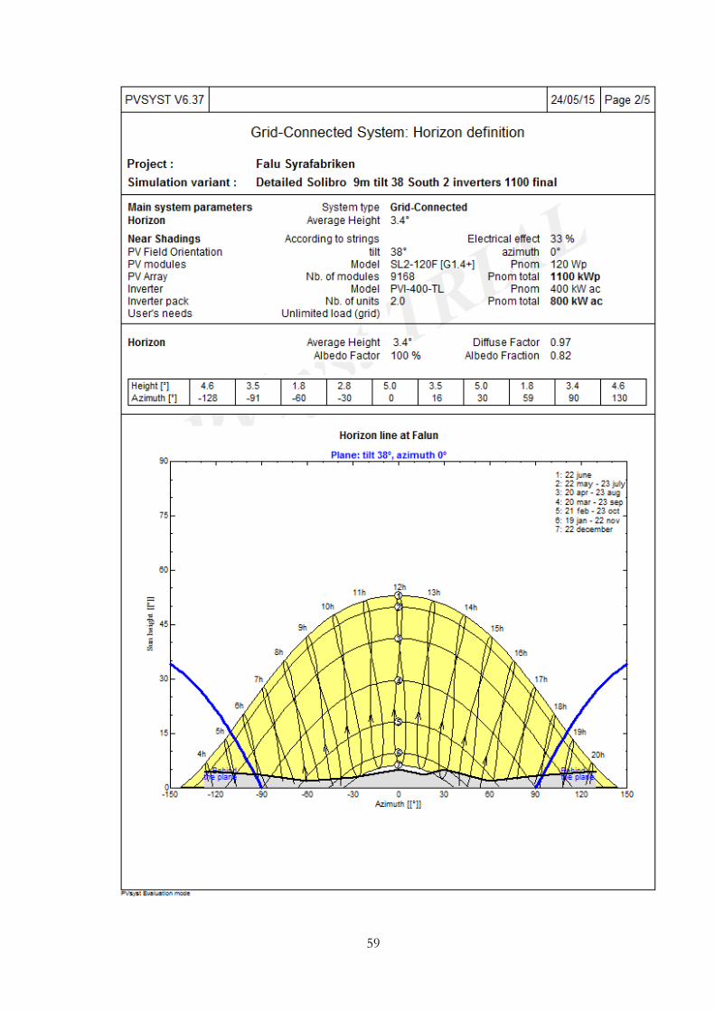
59
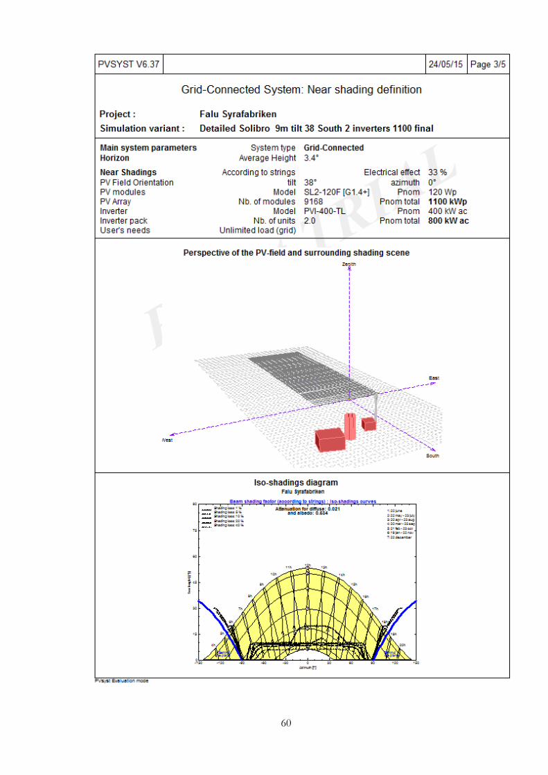
60
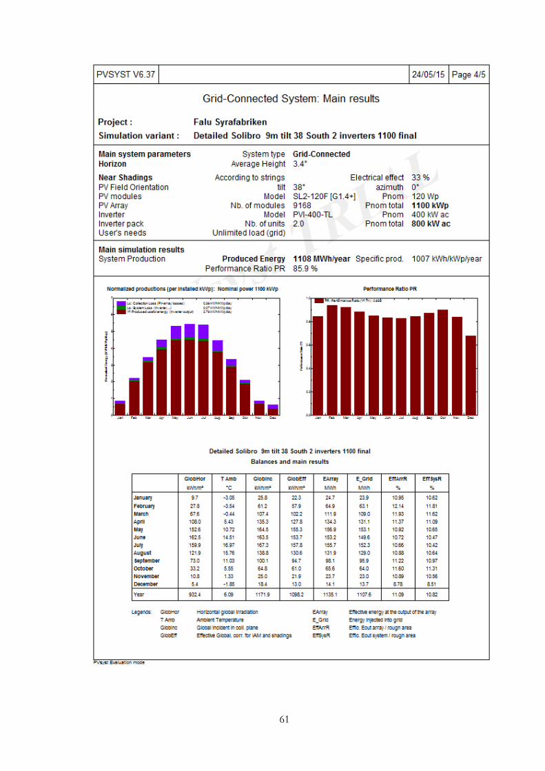
61
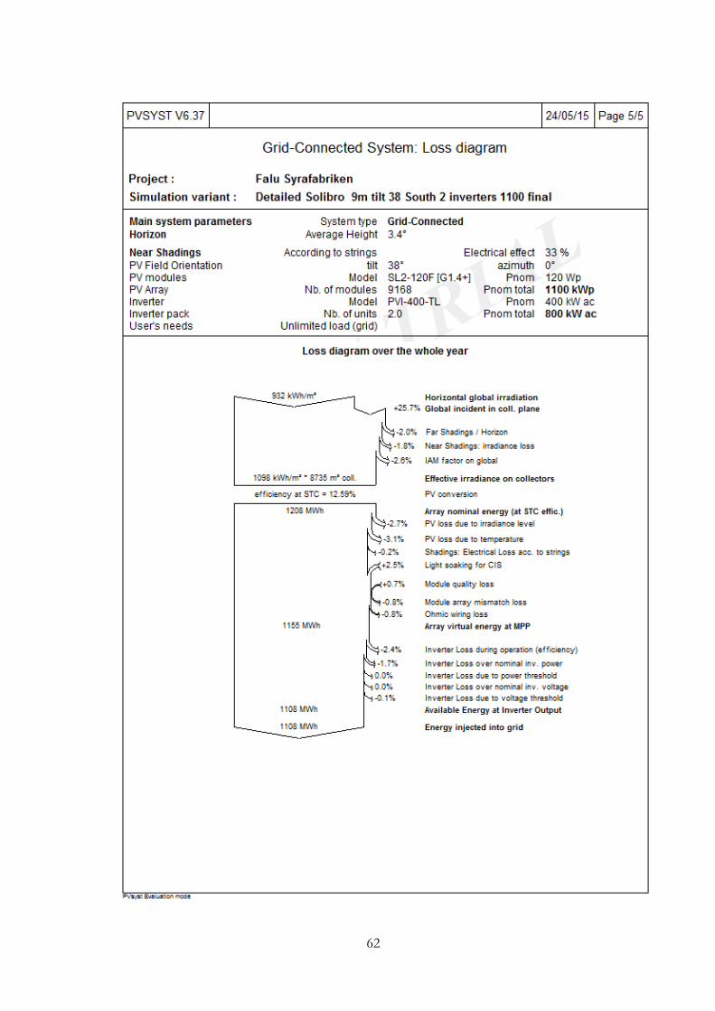
62
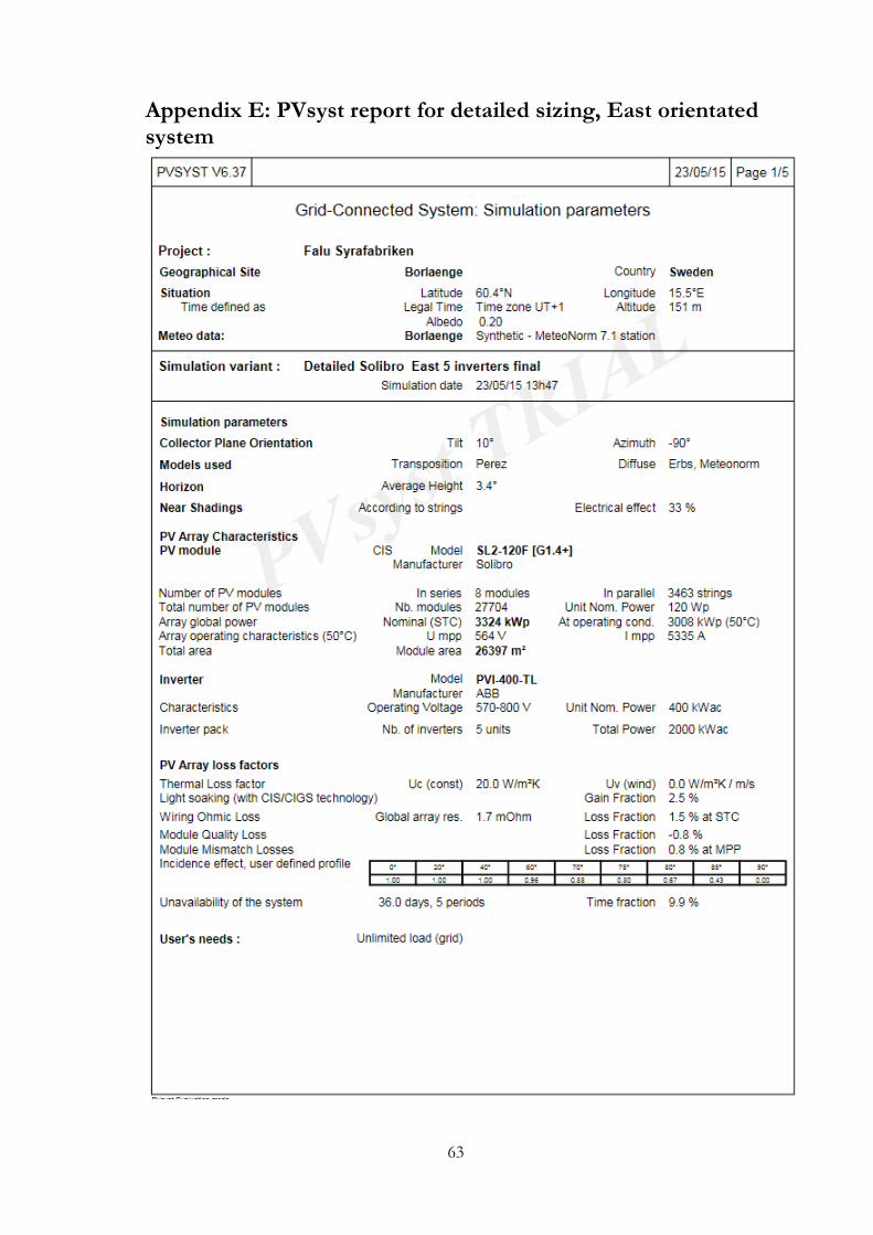
63
Appendix E: PVsyst report for detailed sizing, East orientated system
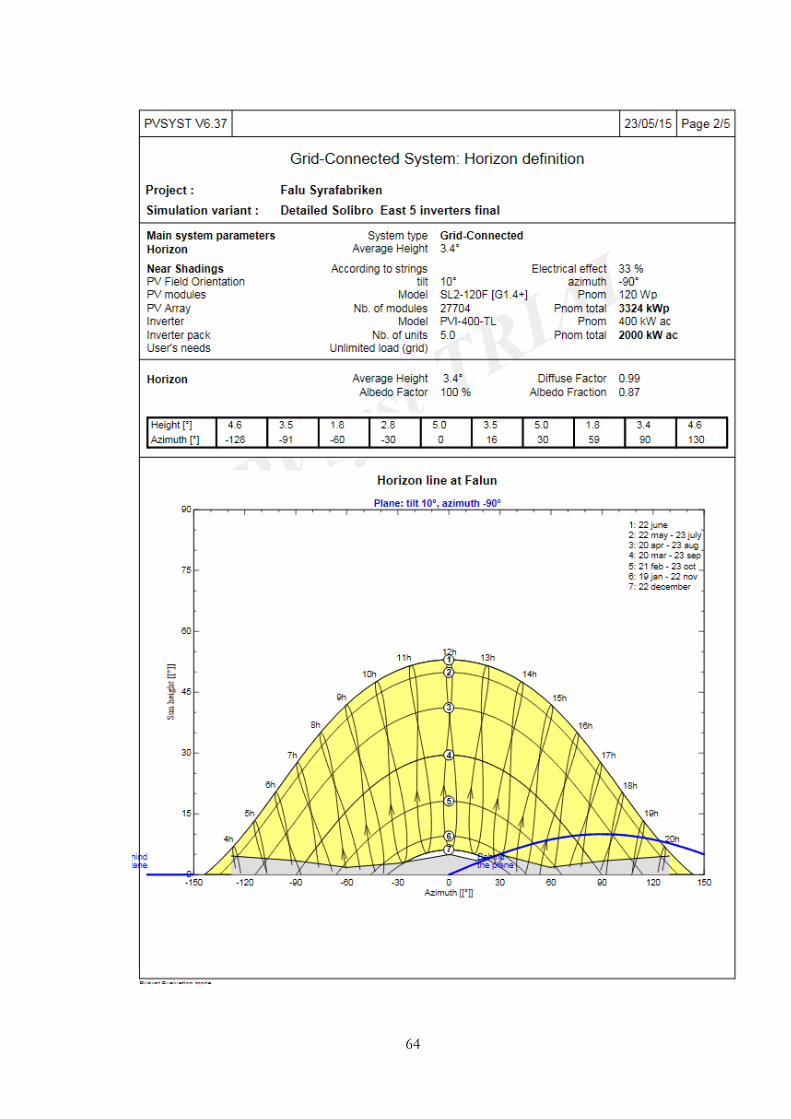
64
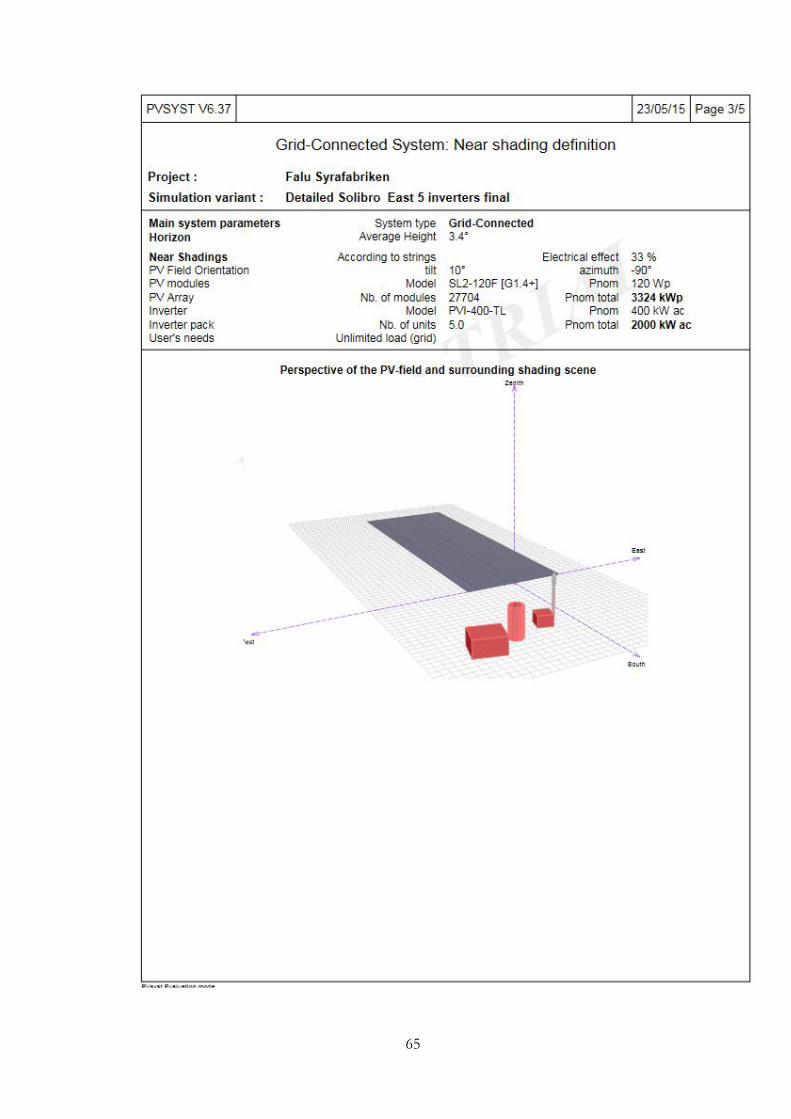
65
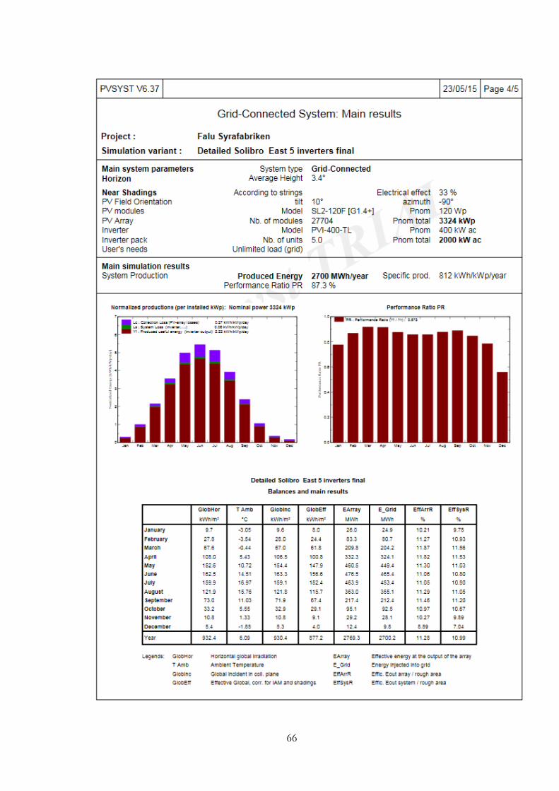
66
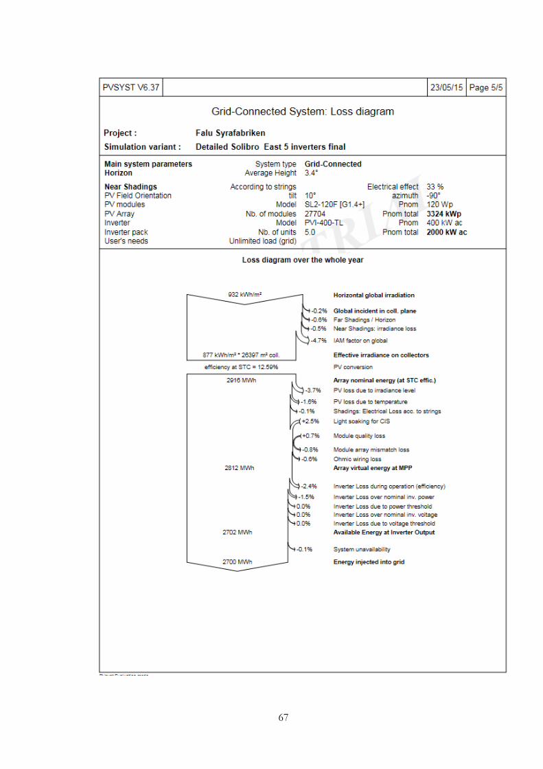
67
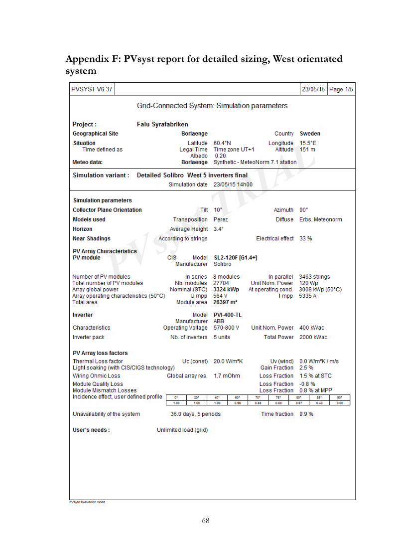
68
Appendix F: PVsyst report for detailed sizing, West orientated system
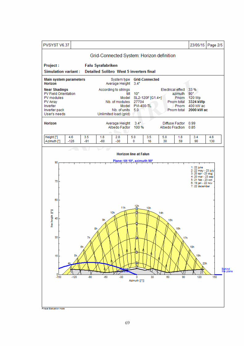
69
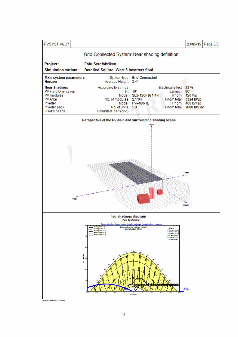
70
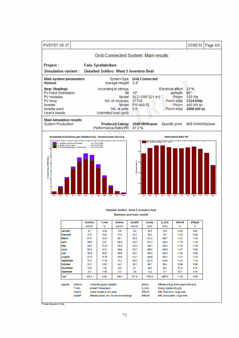
71
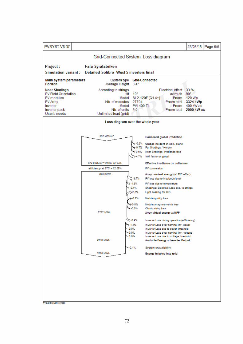
72